High-Dimensional Approximate Nearest Neighbor Search: with Reliable and Efficient Distance Comparison Operations

Abstract.

Approximate K nearest neighbor (AKNN) search in the high-dimensional Euclidean vector space is a fundamental and challenging problem. We observe that in high-dimensional space, the time consumption of nearly all AKNN algorithms is dominated by that of the distance comparison operations (DCOs). For each operation, it scans full dimensions of an object and thus, runs in linear time wrt the dimensionality. To speed it up, we propose a randomized algorithm named ADSampling which runs in logarithmic time wrt the dimensionality for the majority of DCOs and succeeds with high probability. In addition, based on ADSampling we develop one generic and two algorithm-specific techniques as plugins to enhance existing AKNN algorithms. Both theoretical and empirical studies confirm that: (1) our techniques introduce nearly no accuracy loss and (2) they consistently improve the efficiency.

1. Introduction

K nearest neighbor (KNN) search in the high-dimensional Euclidean vector space is a fundamental problem and has a wide range of applications in information retrieval (Liu et al., 2007), data mining (Cover and Hart, 1967) and recommendations (Schafer et al., 2007). However, due to the curse of dimensionality (Indyk and Motwani, 1998), exact KNN query usually requires unacceptable response time. To achieve better time and accuracy tradeoff, many researchers turn to its relaxed version, namely approximate K nearest neighbor (AKNN) search (Datar et al., 2004; Muja and Lowe, 2014; Jegou et al., 2010; Malkov and Yashunin, 2020; Ge et al., 2013; Guo et al., 2020).

Many algorithms have been developed for AKNN, including (1) graph-based (Malkov and Yashunin, 2020; Malkov et al., 2014; Li et al., 2019; Fu et al., 2019, 2021; Iwasaki, 2016), (2) quantization-based (Jegou et al., 2010; Ge et al., 2013; Guo et al., 2020; Gong et al., 2013; Babenko and Lempitsky, 2014, 2015), (3) tree-based  (Muja and Lowe, 2014; Dasgupta and Freund, 2008; Ram and Sinha, 2019; Beygelzimer et al., 2006; Ciaccia et al., 1997) and (4) hashing-based (Indyk and Motwani, 1998; Datar et al., 2004; Gan et al., 2012; Tao et al., 2010; Huang et al., 2015; Sun et al., 2014; Lu et al., 2020; Zheng et al., 2020; Li et al., 2018). In particular, we focus on in-memory AKNN algorithms which assume that all raw data vectors and indexes can be hosted in the main memory (Malkov and Yashunin, 2020; Li et al., 2019; Fu et al., 2019; Malkov et al., 2014; Jegou et al., 2010; Muja and Lowe, 2014; Beygelzimer et al., 2006; Zheng et al., 2020). These algorithms all adopt the strategy of first generating some candidates for KNNs and then finding out the KNNs among them.  First, they differ in their ways of generating candidates of KNNs. For example, graph-based methods organize the vectors with a graph and conduct a heuristic-based search (e.g., greedy search) on the graph for generating candidates. Second, these algorithms largely share their ways of finding KNNs among the candidates. Specifically, they maintain a KNN set $\mathcal{Q}$  (technically, a max-heap), and for a new candidate, they check whether its distance from the query is no greater than the maximum in $\mathcal{Q}$. If so, they include the candidate to $\mathcal{Q}$ with the distance as a key;  otherwise, the candidate is discarded. We call the computation of checking whether an object has its distance from a query no greater than a distance threshold and providing its distance if so a distance comparison operation (DCO). Given an object $\mathbf{o}$ and a distance threshold $r$, we say that $\mathbf{o}$ is a positive object (wrt $r$) if $\mathbf{o}$’s distance from the query is at most $r$ and a negative object otherwise.

All existing AKNN algorithms adopt the following method for the DCO for an object and a threshold. It first computes the object’s distance (from the query) and then compares the computed distance against the threshold. We call this method FDScanning since it scans full dimensions of the object for the operation. Clearly, FDScanning has the time complexity of $O(D)$, where $D$ is the number of dimensions of an object. Based on FDScanning, nearly all AKNN algorithms have their time costs dominated by that of performing DCOs. We consider one of the most popular AKNN algorithms, HNSW (Malkov and Yashunin, 2020), for illustration (elaborations on other algorithms will be provided in Section 2.2). Let $N_{s}$ be the number of generated candidates of KNNs. The total time cost of HNSW is $O(N_{s}D+N_{s}\log N_{s})$, where $O(N_{s}D)$ is the cost of performing DCOs and $O(N_{s}\log N_{s})$ is the cost of other computations (detailed analysis can be found in Section 2.2). Since $D$ can be hundreds while $\log N_{s}$ is a few dozens only for a big dataset involving millions of objects in practice, the cost of performing DCOs dominates the total cost of HNSW (we empirically verify the statement in Section 2.2.). For example, on a real dataset DEEP, which involves 256 dimensions, the DCOs take 77.2% of the total running time.

We have two observations. First, for DCOs on negative objects, we only need to confirm that the objects’ distances are larger than the threshold distance without returning their exact distances - recall that negative objects would be discarded. Therefore, FDScanning, which always computes the distance of an object for a DCO on the object, conducts more than necessary computation for negative objects. Second, among the DCOs involved in an AKNN algorithm, often most would be for negative objects. A clue for this is that when the DCO is conducted on an object, the distance threshold corresponds to some small distance (e.g., the $K$th smallest distance seen so far in many AKNN algorithms). As a result, the object would likely have its distance larger than the threshold and correspond to a negative object. We verify this statement empirically (details can be found in Section 2.2). For example, for a representative algorithm IVF (Jegou et al., 2010), the number of negative objects is 60x to 869x more than that of the positive ones. These observations collectively show that FDScanning is an over-kill for most of the DCOs that are involved for answering a KNN query, and thus there exists much room to achieve reliable (nearly-exact) DCOs  with better efficiency.

In the literature, no efforts have been devoted to achieving reliable DCOs with better efficiency than FDScanning, to the best of our knowledge. An immediate attempt is to use some distance approximation techniques such as product quantization (Ge et al., 2013; Jegou et al., 2010; Gong et al., 2013) and random projection (Johnson and Lindenstrauss, 1984) for DCOs in order to achieve better efficiency. However, as widely found in the literature (Wang et al., 2018; Li et al., 2020) and also empirically verified in our experiments, these techniques cannot avoid accuracy sacrifice in order to achieve some remarkable time cost savings, and thus they can hardly be used to achieve reliable DCOs with better efficiency. For example, according to (Wang et al., 2018), on the dataset SIFT1M with one million 128-dimensional vectors, none of the quantization algorithms achieve more than 60% recall without re-ranking. Indeed, these techniques have only been used for generating candidates of KNNs (Wang et al., 2018), but not (in DCOs) for finding them out from the generated candidates.

Therefore, in this paper, we develop a new method called ADSampling to fulfill this goal. At its core, ADSampling projects the objects to spaces with different dimensionalities and conduct DCOs based on the projected vectors for better efficiency. Different from the conventional random projection technique (Johnson and Lindenstrauss, 1984; Datar et al., 2004; Sun et al., 2014; Gan et al., 2012), which projects all objects to vectors with equal dimensions, ADSampling is novel in the following aspects. First, it projects different objects to vectors with different numbers of dimensions during the query phase flexibly. The rationale is that for negative objects that are farther away from the query, it would be sufficient to project them to a space with fewer dimensions for reliable DCOs; whereas for negative objects that are closer to the query, they should be projected to a space with more dimensions for reliable DCOs. We note that for positive objects (i.e., those that have their distances from the query at most a threshold), their distances should ideally not be distorted. ADSampling achieves this flexibility with two steps. (1) It first preprocesses the objects via a random orthogonal transformation (Choromanski et al., 2017; Jégou et al., 2010) during the index phase (i.e., before a query comes). This step merely randomly rotates the objects without distorting their distances. (2) Then during the query phase, when handling DCOs on different objects, it samples different numbers of dimensions of their transformed vectors. We verify that the sampled vectors produced by these two steps are identically distributed with those obtained from random projection, and thus, the approximate distances based on the sampled vectors, like those based on random projection, correspond to good estimations of the true distances while achieving the aforementioned flexibility of dimensionality.

Second, it decides the number of dimensions to be sampled for each object adaptively based on the DCO on the object during the query phase, but not pre-sets it to a certain number during the index phase (which is knowledge demanding and difficult to set in practice). Specifically, it incrementally samples the dimensions of a transformed vector until it can confidently conduct the DCO on the object based on the sampled vector. With the sampled vector, it determines whether there has been enough evidence for a reliable DCO by computing an approximate distance of the object and then conducting a hypothesis testing based on the computed approximate distance. This is possible due to the fact that there is a theoretical error bound on the approximate distance (recall the aforementioned equivalence between a projected vector by ADSampling and that by the conventional random projection).

ADSampling achieves reliable DCOs with better efficiency than FDScanning, which we explain as follows. First, for each negative object, we prove that ADSampling would always return the correct answer and run in logarithmic time wrt $D$ in expectation (recall that FDSanning runs in linear time wrt $D$). Second, for each positive object, it succeeds with high probability and runs in $O(D)$ time. Third, there are much more negative objects than positive objects.

We summarize the major contributions of this paper as follows.

1. We systematically review existing AKNN algorithms and identify the distance comparison operation (DCO), which is ubiquitous in AKNN algorithms. With the existing method FDScanning, the costs of DCOs dominate the overall costs for nearly all AKNN algorithms, which we verify both theoretically and empirically. (Section 2)

2. We propose a new method ADSampling, which achieves reliable DCOs with better efficiency for the high-dimensional Euclidean space. Specifically, in most of the cases (i.e., for negative objects), ADSampling runs in logarithmic time wrt $D$ and always returns a correct answer. (Section 3)

3. For a general AKNN algorithm (which we denote by AKNN), we replace FDScanning with ADSampling for DCOs and achieve a new algorithm (which we denote by AKNN+). We prove that an AKNN+ algorithm preserves the results of its corresponding AKNN algorithm with high probability and significantly reduces the time complexity. (Section 4)

4. We further develop two AKNN-algorithm-specific techniques to improve the cost-effectiveness of AKNN+ algorithms. For example, for graph-based algorithms (with HNSW+ as a representative), we incorporate more approximations and obtain a new algorithm (which we call HNSW++); for other algorithms (with IVF+ as a representative), we improve their cost-effectiveness with cache-friendly storage. (Section 5)

5. We conduct extensive experiments on real datasets, which verify our techniques. For example, ADSampling brings up to 2.65x speed-up on HNSW and 5.58x on IVF while providing the same accuracy. Besides, it helps to save up to 75.3% of the evaluated dimensions for HNSW and up to 89.2% of those for IVF with the accuracy loss of no more than 0.14%. (Section 6)

For the rest of the paper, we review the related work in Section 7 and conclude the paper in Section 8.

2. The Distance Comparison Operation

2.1. KNN Query and Distance Comparison Operation

Let $\mathcal{O}$ be a database of $N$ objects in a $D$-dimensional Euclidean space $\mathbb{R}^{D}$ and $\mathbf{q}$ be a query. In this paper, we use “object” (resp. “query”) and “data vector” (resp. “query vector”) interchangeably. We note that operations on $\mathcal{O}$ can be conducted before the query $\mathbf{q}$ comes (i.e., the index phase) while those on the query $\mathbf{q}$ can only be conducted after it comes (i.e., the query phase). For an object $\mathbf{o}$, we define its difference from the query $\mathbf{q}$ as $\mathbf{x}$, i.e., $\mathbf{x}=\mathbf{o}-\mathbf{q}$. We refer to an object $\mathbf{o}$ by its corresponding vector $\mathbf{x}$ when the context is clear. Without ambiguity, by “the distance of an object $\mathbf{o}$”, we refer to its distance from the query vector $\mathbf{q}$, which we denote by $dis$. The K nearest neighbor (KNN) query is to find the top-K objects with the minimum distance from the query $\mathbf{q}$.

In this paper, we study the distance comparison operation (DCO), which is defined as follows.

Definition 2.1 (Distance Comparison Operation).

Given an object $\mathbf{o}$ and a distance threshold $r$, the distance comparison operation (DCO) is to decide whether object $\mathbf{o}$ has its distance $dis$ no greater than $r$ and if so, return $dis$. In particular, we say object $\mathbf{o}$ is a positive object if $dis\leq r$ and a negative object otherwise.

As mentioned in Section 1, DCOs are heavily involved in many AKNN algorithms. These algorithms conduct the DCO for an object $\mathbf{o}$ and a distance $r$ naturally by computing $\mathbf{o}$’s distance and comparing the distance against $r$. We call this conventional method FDScanning since it uses all dimensions of $\mathbf{o}$ for computing the distance. Clearly, FDScanning has the time complexity of $O(D)$.

Next, we review the existing AKNN algorithms and validate both theoretically and empirically the critical role of DCOs in these algorithms.

2.2. AKNN Algorithms and Their DCOs

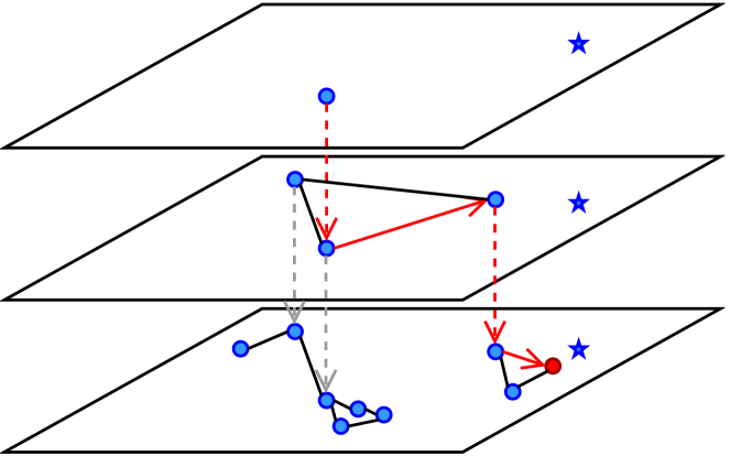
((a)) HNSW

((b)) IVF

Figure 1. Illustrations of AKNN algorithms.

2.2.1. Graph-Based Methods

Graph-based methods are one family of state-of-the-art AKNN algorithms that exhibit dominant performance on the time-accuracy tradeoff for in-memory AKNN query (Malkov and Yashunin, 2020; Malkov et al., 2014; Li et al., 2019; Fu et al., 2019, 2021; Iwasaki, 2016). These methods construct graphs based on the data vectors, where a vertex corresponds to a data vector. One famous graph-based method is the hierarchical navigable small world graphs (HNSW) (Malkov and Yashunin, 2020). It’s composed of several layers. Layer 0 (base layer) contains all data vectors and layer $i+1$ only keeps a subset of the vectors in layer $i$ randomly. The size of each layer decays exponentially as it goes up. In particular, the top layer contains only one vertex. Within each layer, a vertex is connected to its several approximate nearest neighbors, while between adjacent layers, two vertexes are connected only if they represent the same vector. An illustration of the HNSW graph is provided in Figure 1(a).

During the query phase, greedy search is first performed on upper layers to find a good entry at layer 0 (the base layer). Specifically, the search starts from the only vertex of the top layer. Within each layer, it does greedy search iteratively. At each iteration, it accesses all the neighbors of its currently located vertex and goes to the one with the minimum distance. It terminates the search when none of the neighbors has a smaller distance than the currently located vertex. Then it goes to the next layer and repeats the process until it arrives at layer 0. At layer 0, it conducts greedy beam search (Wang et al., 2021a) (best first search), which is adopted by most graph-based methods (Malkov and Yashunin, 2020; Li et al., 2019; Fu et al., 2019; Jayaram Subramanya et al., 2019; Malkov et al., 2014). To be specific, greedy beam search maintains two sets: a search set $\mathcal{S}$ (a min-heap by exact distances) and a result set $\mathcal{R}$ (a max-heap by exact distances). The search set $\mathcal{S}$ has its size unbounded and maintains candidates yet to be searched. The result set $\mathcal{R}$ has its size bounded by $N_{ef}$ and maintains $N_{ef}$ nearest neighbors visited so far, where the size $N_{ef}$ is the parameter to control time-accuracy trade-off. At the beginning, a start point at layer 0 is inserted into both $\mathcal{S}$ and $\mathcal{R}$. Then it proceeds in iterations. At each iteration, it pops the object with the smallest distance in set $\mathcal{S}$ and enumerates the neighbors of the object. For each neighbor, it checks whether its distance from the query object is no greater than the maximum distance in set $\mathcal{R}$ and if so, it computes the distance (i.e., it conducts a DCO). In addition, if the distance is smaller than the maximum distance in $\mathcal{R}$, it (1) pushes the object into both set $\mathcal{S}$ and set $\mathcal{R}$ (using the computed distance as the key) and (2) pops the object with the maximum distance from set $\mathcal{R}$ whenever $\mathcal{R}$ involves more than $N_{ef}$ objects so that the size of $\mathcal{R}$ is bounded by $N_{ef}$. It returns $K$ objects in $\mathcal{R}$ with the smallest distances when the minimum distance in $\mathcal{S}$ becomes larger than the maximum distance in $\mathcal{R}$ and stops. We note that the greedy search at upper layers corresponds to a greedy beam search process with $N_{ef}=1$.

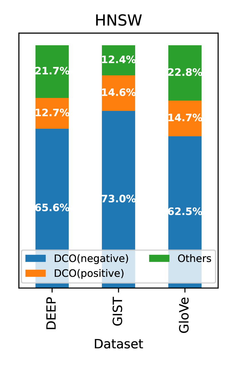
((a)) HNSW

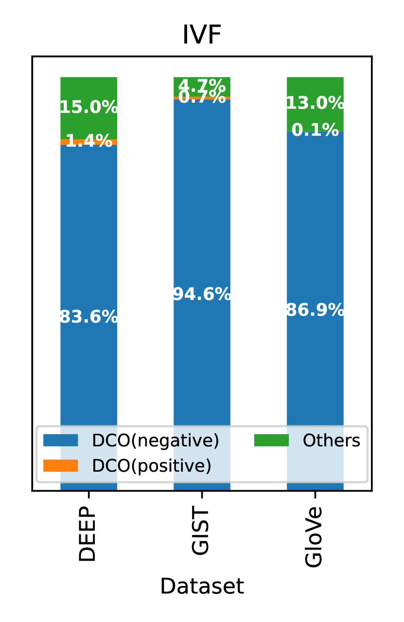
((b)) IVF

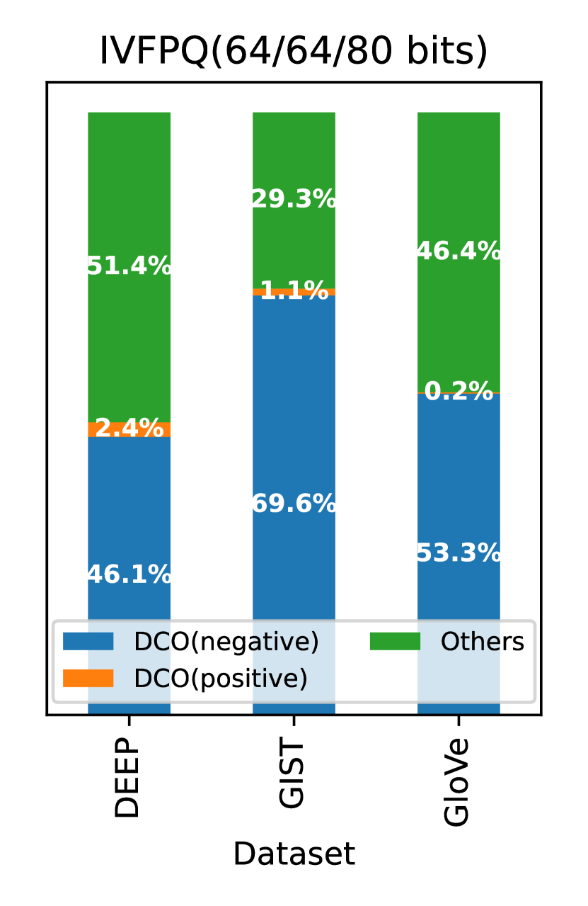
((c)) IVFPQ

Figure 2. Breakdown of Running Times of AKNN Algorithms.

DCO v.s. Overall Time Costs. We review the time complexity of HNSW assuming that it adopts FDScanning for DCOs. Let $N_{s}$ be the number of the candidates of KNN objects, which are visited by HNSW. Then, the total cost of the DCOs is $O(N_{s}D)$ and that of updating the sets $\mathcal{S}$ and $\mathcal{R}$ is $O(N_{s}\log N_{s})$. Therefore, the time complexity of HNSW is $O(N_{s}D+N_{s}\log N_{s})$. In practice, the total cost of DCOs should be the dominating part since $D$ can be hundreds while $\log N_{s}$ is a few dozens only for a big dataset involving millions of objects. We verify this empirically as well. Figure 2(a) profiles the time consumption of HNSW on three real-world datasets when targeting 95% recall with $K=100$. According to the results, on datasets with various dimensions from 256 to 960, DCOs take from 77.2% to 87.6% of the total running time of HNSW (as indicated by the blue and orange portions of the bars).

Positive v.s. Negative Objects. We verify empirically that for HNSW, the number of DCOs on negative objects is significantly larger than that of DCOs on positive objects. The results are shown in Figure 2(a). We note that in the figure, the ratio between the cost of DCOs (on negative objects) and that (on positive objects) reflects the ratio between the numbers of negative and positive objects since a DCO on a negative object and that on a positive object have the same cost. According to the results, the number of negative objects is 4.3x to 5.2x times more than that of the positive ones.

2.2.2. Inverted File Index

Inverted file (Jegou et al., 2010) index is another popular index method for AKNN query. According to (Li et al., 2020), IVF is one of the state-of-the-art approaches for AKNN. Indeed, according to our experimental results in Section 6.2, it outperforms HNSW on some datasets. During the index phase, the algorithm clusters data vectors with the K-means algorithm, builds a bucket for each cluster and assigns each data vector to its corresponding bucket. Then during the query phase, for a given query, the algorithm first selects the $N_{probe}$ nearest clusters based on their centroids, retrieves all vectors in these corresponding buckets as candidates, and then finds out KNNs among the retrieved vectors. Here, $N_{probe}$ is a user parameter which controls the time-accuracy trade-off. When finding out KNNs, a commonly used method is to maintain a KNN set $\mathcal{K}$ with a max-heap of size $K$. It then scans all candidates, and for each one, it checks whether its distance is no greater than the maximum of $\mathcal{K}$ and if so, it computes the distance (i.e., it conducts a DCO). Here, the maximum distance is defined to be $+\infty$ if $\mathcal{K}$ is not full. If the distance is smaller than the maximum distance in $\mathcal{K}$, it updates $\mathcal{K}$ with the candidate (by using the computed distance as the key). It returns the objects in $\mathcal{K}$ at the end. An illustration of the IVF structure is provided in Figure 1(b).

DCO v.s. Overall Time Costs. We review the time complexity of IVF assuming that it adopts FDScanning for DCOs. Let $N_{s}$ be the number of candidate objects. The total cost of IVF is $O(N_{s}D+N_{s}\log K)$, where the first term is the cost of the DCOs and the second term is that of updating $\mathcal{K}$. As can be noticed, the cost of DCOs is the dominating part. We verify this empirically as we did for HNSW. Figure 2(b) shows the results. According to the results, on datasets with various dimensions from 256 to 960, DCOs take from 85.0% to 95.3% of the total running time of IVF.

Positive v.s. Negative Objects. We verify empirically that for IVF, the number of DCOs on negative objects is significantly larger than that of DCOs on positive objects. The results are shown in Figure 2(b). According to the results, the number of negative objects is 60x to 869x more than that of the positive ones.

2.2.3. Other AKNN Algorithms

In other AKNN algorithms including tree-based, hashing-based, and quantization-based methods, DCOs are also ubiquitous. Tree-based methods (Muja and Lowe, 2014; Dasgupta and Freund, 2008; Ram and Sinha, 2019; Beygelzimer et al., 2006; Ciaccia et al., 1997) generate candidate vectors through tree routing and find out KNNs with DCOs (similarly as IVF does). Hashing-based methods (Indyk and Motwani, 1998; Datar et al., 2004; Gan et al., 2012; Tao et al., 2010; Huang et al., 2015; Sun et al., 2014; Lu et al., 2020; Zheng et al., 2020) generate candidate vectors via hashing codes and find out KNNs with DCOs (similarly as IVF does). Quantization-based methods (Jegou et al., 2010; Wang et al., 2016; Ge et al., 2013; Gong et al., 2013; Babenko and Lempitsky, 2015, 2014) generate candidates with short quantization codes, and conduct re-ranking (for finding out KNNs) with DCOs (similarly as IVF does). For tree-based and hashing-based methods, the cost of DCOs is dominant because (1) one time tree routing or hashing bucket probing generates multiple candidates (which entail multiple DCOs) and (2) tree routing and hashing bucket probing are much faster than a DCO (which has the time complexity of $O(D)$). For product quantization-based methods (Jegou et al., 2010; Ge et al., 2013; Gong et al., 2013; Babenko and Lempitsky, 2015), DCOs are involved in its re-ranking stage, which is less dominant because the main cost lies in evaluating quantization codes. For comparison, we show the time decomposition results of IVFPQ, which is a quantization-based method (Jegou et al., 2010), in Figure 2(c) under the typical setting of (Wang et al., 2016; Jegou et al., 2010).

3. The ADSampling Method

Recall that our goal is to achieve reliable DCOs with better efficiency than FDScanning. To this end, we develop a new method called ADSampling. At its core, ADSampling projects the objects to vectors with fewer dimensions and conduct DCOs based on the projected vectors for better efficiency. Different from the conventional and widely-adopted random projection technique (Johnson and Lindenstrauss, 1984; Datar et al., 2004; Sun et al., 2014; Gan et al., 2012), which projects all objects to vectors with equal dimensions, ADSampling is novel in the following aspects. First, it projects different objects to vectors with different numbers of dimensions during the query phase flexibly. We will elaborate on details of how this idea is implemented in Section 3.1. Second, it decides the number of dimensions to be sampled for each object adaptively based on the DCO on the object during the query phase, but not pre-sets it to a certain number during the index phase (which is knowledge demanding and difficult to set in practice). We will elaborate on details of how this idea is implemented in Section 3.2. In addition, we summarize ADSampling and prove that it has its time logarithmic wrt $D$ for negative objects (which is significantly better than the time complexity $O(D)$ of FDScanning) in Section 3.3.

3.1. Dimension Sampling over Randomly Transformed Vectors

For better efficiency of a DCO, a natural idea is to conduct a random projection (Johnson and Lindenstrauss, 1984; Vershynin, 2018) on an object (i.e., to multiply the object (specifically its vector) with a $\mathbb{R}^{d\times D}$ random matrix $P$ where $d<D$ ), and then conduct the DCO using the approximate distance that can be computed based on the projected vector, namely $\sqrt{D/d}\|P\mathbf{x}\|$. It is well-known that there exists a concentration inequality on the approximate distance as presented in the following lemma (Vershynin, 2018).

Lemma 3.1.

For a given object $\mathbf{x}\in\mathbb{R}^{D}$, a random projection $P\in\mathbb{R}^{d\times D}$ preserves its Euclidean norm with $\epsilon$ multiplicative error bound with the probability of

(1) $$\mathbb{P}\left\{\left|\sqrt{\frac{D}{d}}\|P\mathbf{x}\|-\|\mathbf{x}\|\right|\leq\epsilon\|\mathbf{x}\|\right\}\geq 1-2e^{-c_{0}d\epsilon^{2}}$$

where $c_{0}$ is a constant factor and $\epsilon\in(0,+\infty)$.

Nevertheless, once an object is projected, the corresponding approximate distance would have a certain resolution that would be fixed. Therefore, it lacks of flexibility of achieving different reduced dimensionalities for different objects (correspondingly different resolutions of approximate distances) during the query phase.

We aim to project different objects to vectors with different numbers of dimensions during the query phase flexibly. To this end, we propose to randomly transform an object (with random orthogonal transformation (Johnson and Lindenstrauss, 1984; Vershynin, 2018; Gong et al., 2013), geometrically, to randomly rotate it) and then flexibly sample dimensions of the transformed vector for computing an approximate distance. Formally, given an object $\mathbf{x}$, we first apply a random orthogonal matrix $P^{\prime}\in\mathbb{R}^{D\times D}$ to $\mathbf{x}$ and then sample $d$ rows on it (for simplicity, the first $d$ rows). The result is denoted by $(P^{\prime}\mathbf{x})|_{[1,2,...,d]}$. This method entails two benefits. First, we achieve the flexibility since we can sample $d$ dimensions of a rotated vector for different $d$’s during the query phase. Second, we achieve a guaranteed error bound since sampling $d$ dimensions on a transformed vector is equivalent to obtaining a $d$-dimensional vector via random projection, which we explain as follows.

Recall that a random projection on $\mathbf{x}$ is to apply a random projection matrix $P\in\mathbb{R}^{d\times D}$ to $\mathbf{x}$, and the result is denoted by $P\mathbf{x}$. We claim that $(P^{\prime}\mathbf{x})|_{[1,2,...,d]}$ (the result of our proposed method) and $P\mathbf{x}$ (the result of a random projection) are identically distributed. This is based on an elementary property of matrix multiplication that row samplings before and after a matrix multiplication are identical:

(2) $$(P^{\prime}\mathbf{x})|_{[1,2,...,d]}=P^{\prime}|_{[1,2,...,d]}\mathbf{x}$$

We note that $P^{\prime}|_{[1,2,...,d]}$ corresponds to a random matrix $P$ for random projection since one conventional way to generate a random projection matrix $P$ is to sample rows of a $D\times D$ random orthogonal matrix (Choromanski et al., 2017). Therefore, the concentration inequality for random projection over raw objects (as given in Equation (1)) can be applied to dimension sampling over randomly transformed vectors, which provides solid foundation for our following discussion.

We denote the transformed vector as $\mathbf{y}:=P^{\prime}\mathbf{x}$. Based on the sampled dimensions, we can compute an approximate distance of $\mathbf{x}$, denoted by $dis^{\prime}$, as follows,

(3) $$dis^{\prime}:=\sqrt{\frac{D}{d}}\left\|\mathbf{y}|_{[1,2,...,d]}\right\|$$

where $d$ is the number of sampled dimensions. We note that the time complexity of computing an approximate distance based on $d$ sampled dimensions is $O(d)$. Furthermore, when all $D$ dimensions are sampled, the distance $dis^{\prime}$ computed based on the sampled dimensions would be equal to the true distance $dis$, which is due to the fact that random orthogonal transformation preserves the norm of any vector (since it simply rotates the space without distorting the distances).

3.2. Incremental Sampling with Hypothesis Testing

One remaining issue is how to determine the number of dimensions of $\mathbf{y}$ we need to sample in order to make a sufficiently confident conclusion for the DCO (i.e., to decide whether $dis\leq r$). Intuitively, with more sampled dimensions, the approximate distance $dis^{\prime}$ would be more accurate, and we would be able to make a more confident conclusion. On the other hand, sampling more dimensions would result in higher cost of computing the approximate distance (since the cost is linear wrt the number of sampled dimensions). We aim to sample the minimum possible number of dimensions, which are sufficient to make a confident conclusion.

Specifically, we propose to sample the dimensions of $\mathbf{y}$ in an incremental manner, i.e., we start with a few dimensions. If with the current sampled dimensions, we cannot make a confident conclusion, we continue to sample some more until we can make a confident conclusion or we have sampled all dimensions. As a result, the problem reduces to the one of deciding whether we can make a sufficiently confident conclusion with a certain, say $d$, sampled dimensions? In a statistics language, the observed distance $dis^{\prime}$ (computed based on the sampled dimensions) is an estimator of the true distance $dis$ and its distribution depends only on the true value $dis$ and the number of sampled dimensions $d$. The task is to draw a conclusion about a true value $dis$ (i.e., whether $dis\leq r$) with an observed value $dis^{\prime}$. It’s exactly what hypothesis testing typically does. Motivated by this, we propose to leverage hypothesis testing to solve the problem. Specifically, we conduct the hypothesis testing as follows.

1. We define a null hypothesis $H_{0}:dis\leq r$ and its alternative $H_{1}:dis>r$.

2. We use $dis^{\prime}$ as the estimator of $dis$. The relationship between $dis^{\prime}$ and $dis$ is provided in Lemma 3.1 (i.e., the difference between $dis^{\prime}$ and $dis$ is bounded by $\epsilon\cdot dis$ with the failure probability at most $2\exp(-c_{0}d\epsilon^{2})$).

3. We set the significance level $p$ to be $2\exp(-c_{0}\epsilon_{0}^{2})$, where $\epsilon_{0}$ is a parameter to be tuned empirically. With this, the event that the observed $dis^{\prime}$ is much larger than $r$ (i.e., $dis^{\prime}>(1+\epsilon_{0}/\sqrt{d})\cdot r$) has its probability below the significance level $p$ (which can be verified based on Lemma 3.1 with $\epsilon=\epsilon_{0}/\sqrt{d}$ and $H_{0}:dis\leq r$).

4. We check whether the event happens ($dis^{\prime}>(1+\epsilon_{0}/\sqrt{d})\cdot r$). If so, we can reject $H_{0}$ and conclude $H_{1}:dis>r$ with sufficient confidence; otherwise, we cannot.

There are three cases for the outcome of the hypothesis testing. Case 1: we reject the hypothesis (i.e., we conclude $dis>r$) and $d<D$. In this case, the time cost (which is mainly for evaluating the approximate distance) is $O(d)$, which is smaller than that of computing the true distance in $O(D)$ time. Case 2: we cannot reject the hypothesis and $d<D$. In this case, we would continue to sample some more dimensions of $\mathbf{y}$ incrementally and conduct another hypothesis testing. Case 3: $d=D$. In this case, we have sampled all dimensions of $\mathbf{y}$ and the approximate distance based on the sampled vector is equal to the true distance. Therefore, we can conduct an exact DCO. We note that the incremental dimension sampling process with (potentially sequential) hypothesis testing would have its time cost strictly smaller than $O(D)$ (when it terminates in Case 1) and equal to $O(D)$ (when it terminates in Case 3).

We note that hypothesis testing has also been used for deciding a certain number of hashes for LSH in the context of similarity search (Chakrabarti and Parthasarathy, 2015; Satuluri and Parthasarathy, 2011). The differences between our technique and (Chakrabarti and Parthasarathy, 2015; Satuluri and Parthasarathy, 2011) include: (1) ours is based on a random process of sampling dimensions of a transformed vector while (Chakrabarti and Parthasarathy, 2015; Satuluri and Parthasarathy, 2011) are on one of sampling hash functions, which entail significantly different hypothesis testings and (2) ours targets the Euclidean distance function while (Chakrabarti and Parthasarathy, 2015; Satuluri and Parthasarathy, 2011) target similarity functions such as Jaccard and Cosine similarity measures (it remains non-trivial to adapt the latter to the Euclidean space), and (3) ours guarantees to be no worse than the method of evaluating exact distances (in our case, i.e., FDScanning) because it obtains exact distances when it has sampled all the dimensions while (Chakrabarti and Parthasarathy, 2015; Satuluri and Parthasarathy, 2011) have no such guarantee (when they have sampled all the hash functions and still cannot produce a firmed result, they would have to re-evaluate exact similarities from scratch).

3.3. Summary and Theoretical Analysis

Summary. We summarize the process of ADSampling in Algorithm 1. It takes a transformed data vector $\mathbf{o}^{\prime}$, a transformed query vector $\mathbf{q}^{\prime}$ and a distance threshold $r$ as inputs and outputs the result of the DCO of whether $dis\leq r$: 1 for yes (in this case, it returns $dis$ as well) and 0 for no. We note that the transformation of the data vectors is conducted in the index phase and its cost can be amortized by all the subsequent queries on the same database. The transformation of the query vector is conducted in the query phase when a query comes and its cost can be amortized by all the DCOs involved for answering the same query. Specifically, the algorithm maintains the number of sampled dimensions with a variable $d$ with $d=0$ initially (line 1). It then performs an iterative process if $d<D$ (line 2). At each iteration, it samples some more dimensions incrementally and updates $d$ and the approximate distance $dis^{\prime}$ accordingly (line 3-4) and conducts a hypothesis testing with the null hypothesis as $dis\leq r$ based on the approximate distance $dis^{\prime}$ (line 5). It then returns the result in three cases as explained in Section 3.2 (line 6 - 11).

Input : A transformed data vector $\mathbf{o}^{\prime}$, a transformed query vector $\mathbf{q}^{\prime}$ and a distance threshold $r$

Output : The result of DCO (i.e., whether $dis\leq r$): 1 means yes and 0 means no; In case of the result of 1, an exact distance is also returned

1 Initialize the number of sampled dimensions $d$ to be 0

2 while $d<D$ do

3       Sample some more dimensions $y_{i}$ incrementally with $y_{i}=\mathbf{o}_{i}^{\prime}-\mathbf{q}_{i}^{\prime}$

4       Update $d$ and the approximate distance $dis^{\prime}$ accordingly

5       Conduct a hypothesis testing with the null hypothesis $H_{0}$ as $dis\leq r$ based on the approximate distance $dis^{\prime}$

6       if $H_{0}$ is rejected and $d<D$ then // Case 1

7             return 0

8            

9      else if $H_{0}$ is not rejected and $d<D$ then // Case 2

10             continue

11            

12      else  // Case 3

13             return 1 (and $dis^{\prime}$) if $dis^{\prime}\leq r$ and 0 otherwise

14            

15      

Algorithm 1 ADSampling

Failure Probability Analysis. Note that ADSampling terminates in either Case 1 (with the hypothesis being rejected and $d<D$) or Case 3 (with $d=D$). When it terminates in Case 3, there would be no failure since in this case, the approximate distance $dis^{\prime}$ is equal to the true distance $dis$ and the DCO result is exact. When it terminates in Case 1, a failure would happen if $dis\leq r$ holds since in this case, it concludes that $dis>r$ (by rejecting the null hypothesis). We analyze the probability of the failure. As discussed in Section 3.2, we can control the failure probability with $\epsilon_{0}$. The following lemma presents the relationship between $\epsilon_{0}$ and the failure probability of a DCO with ADSampling.

Lemma 3.2.

For a DCO in $D$-dimensional space, the failure probability of ADSampling is given by

(4) $$\mathbb{P}\left\{{failure}\right\}=0{\text{~{}~{}if $dis>r$}}$$

(5) $$\mathbb{P}\left\{{failure}\right\}\leq\exp\left(-c_{0}\epsilon_{0}^{2}+\log D\right){\text{~{}~{}if $dis\leq r$}}$$

Proof.

The correctness for the case of $dis>r$ is obvious and that of the other case ($dis\leq r$) can be verified as follows.

(6) $$\mathbb{P}\left\{{failure}\right\}=\mathbb{P}\left\{\exists d<D,dis^{\prime}>(1+\epsilon_{0}/\sqrt{d})\cdot r\right\}$$

(7) $$\leq \sum_{d=1}^{D-1}\mathbb{P}\left\{dis^{\prime}>(1+\epsilon_{0}/\sqrt{d})\cdot dis\right\}$$

(8) $$\leq \sum_{d=1}^{D-1}\exp\left(-c_{0}\epsilon_{0}^{2}\right)\leq\exp\left(-c_{0}\epsilon_{0}^{2}+\log D\right)$$

where (6) is because a failure happens if and only if we accidentally reject the hypothesis for some $d<D$; (7) applies union bound and the fact that $dis\leq r$; and (8) is due to Lemma 3.1. ∎

Time Complexity Analysis. Let $\hat{D}$ be the number of sampled dimensions by ADSampling. Clearly, the time complexity ADSampling is $O(\hat{D})$. Given the stochastic nature of the method, $\hat{D}$ is a random variable. Next, we analyze the expectation of $\hat{D}$, denoted by $\mathbb{E}[\hat{D}]$. First of all, since $\hat{D}$ is always at most $D$, we know $\mathbb{E}[\hat{D}]\leq D$. Furthermore, for the DCO on a negative object with $dis>r$, we can derive that $\mathbb{E}[\hat{D}]$ relies on $\epsilon_{0}$ and $\alpha=(dis-r)/r$ (which we call the distance gap between $dis$ and $r$), as presented below (detailed proof can be found in Appendix A).

Lemma 3.3.

When ADSampling is used for the DCO on an object and a threshold $r$ with $dis>r$, letting $\alpha=(dis-r)/r$, we have

(9) $$\mathbb{E}\left[\hat{D}\right]=O\left[\min\left(D,\alpha^{-2}\cdot\epsilon_{0}^{2}\right)\right]$$

The above result is well aligned with the intuitions that (1) when the distance gap between $dis$ and $r$, i.e., $(dis-r)/r$, is larger, fewer dimensions would be sampled for making a sufficiently confident conclusion and (2) when $\epsilon_{0}$ is larger (i.e., the significance value of the hypothesis testings is smaller, which means a higher requirement on the confidence), more dimensions would be sampled.

We further derive the time-accuracy trade-off of ADSampling.

Theorem 3.4.

When ADSampling is used for the DCO on an object and a threshold $r$ with $dis>r$, letting $\alpha=(dis-r)/r$, we have

(10) $$\mathbb{E}\left[\hat{D}\right]=O\left[\min\left(D,\frac{1}{\alpha^{2}}\log\frac{D}{\delta}\right)\right]$$

for achieving its failure probability (of positive objects) at most $\delta$.

Proof.

Making the failure probability in Lemma 3.2 be equal to $\delta$, we obtain the corresponding $\epsilon_{0}$. Then by substituting $\epsilon_{0}$ in Lemma 3.3, we have the theorem. ∎

ADSampling v.s. FDScanning. Compared with FDScanning, ADSampling improves the complexity for negative objects from being linear to being logarithmic wrt $D$ at the cost of the accuracy for positive objects (Theorem 3.4). We emphasize that the failure probability (of positive objects) decays quadratic-exponentially (Lemma 3.2) while the time complexity (of negative objects) grows quadratically (Lemma 3.3), both with respect to $\epsilon_{0}$. It indicates that to achieve nearly-exact DCOs, we only need sample a few dimensions. We empirically verify these results in Section 6.2.6. It shows that with ADSampling as a plugin, an exact KNN algorithm, namely linear scan, needs only on average 55 dimensions per vector on GIST (originally 960 dimensions) to achieve ¿99.9% recall.

4. AKNN+: Improving AKNN Algorithms with ADSampling as a Plug-in Component

Recall that an AKNN algorithm, which we denote by AKNN and could be any one among many existing algorithms (Malkov and Yashunin, 2020; Jegou et al., 2010; Muja and Lowe, 2014; Fu et al., 2019; Datar et al., 2004), involves many DCOs. In the literature, FDScanning is typically adopted for DCOs and runs in $O(D)$ time. Given that ADSampling can conduct reliable DCOs with better efficiency, a natural idea is to improve the AKNN algorithms by adopting ADSampling for the DCOs. Specifically, since ADSampling is based on randomly transformed data vectors and query vectors, before any query comes, we randomly transform all data vectors, and when a query comes, we randomly transform the query vector. Then, we run the AKNN algorithm based on the transformed data and query vectors. Recall that the time cost of transforming the data vectors can be amortized across different queries and the time cost of transforming the query vector can be amortized across many different DCOs involved for answering the query. During the running process of the AKNN algorithm, whenever it conducts a DCO, we use the ADSampling method. For example, for graph-based methods such as HNSW, we use the ADSampling method when comparing the distance of a newly visited object with the maximum in the result set $\mathcal{R}$. For other AKNN algorithms such as IVF, we apply ADSampling when comparing the distance of a candidate and the maximum in the currently maintained KNN set $\mathcal{K}$ for selecting the final KNNs from the generated candidates.

For an AKNN algorithm AKNN, which adopts ADSampling for DCOs, we call it AKNN+. For example, we call HNSW and IVF with ADSampling adopted for DCOs HNSW+ and IVF+, respectively.

Theoretical Analysis. Recall that ADSampling improves the efficiency of DCOs on negative objects at the cost of the accuracy of those on positive objects. We show the relationship between the probability that AKNN+ fails to return the same results as AKNN and the time complexity of the DCO on a negative object involved in AKNN+ below. Basically, to preserve the returned results of AKNN, it suffices to produce correct results for all DCOs, whose number is at most $N$. Then with union bound, the failure probability of AKNN+ is upper bounded by the sum of the failure probability of each single DCO. Thus, making the failure probability of ADSampling be $\delta=\delta^{\prime}/N$ yields the following corollary.

Corollary 4.1.

Let $\delta^{\prime}$ be the probability that AKNN+ fails to return the same results as AKNN. The expected time complexity of the DCO on a negative object with distance gap $\alpha$ is reduced to

(11) $$\mathbb{E}\left[\hat{D}\right]=O\left[\min\left(D,\frac{1}{\alpha^{2}}\log\frac{DN}{\delta^{\prime}}\right)\right]$$

and the remaining time cost (for DCOs on positive objects and other computations) is unchanged.

Furthermore, for those AKNN+ algorithms which generate candidates all at once (e.g., IVF), producing correct DCO results for KNN objects ($K$ objects) rather than for all objects (at most $N$ objects) is sufficient to return the same results as its corresponding AKNN algorithm. This is because once we produce correct results for the DCOs on the true KNN objects, we also obtain their exact distances (note that all of them would be positive objects). It ensures to return them as the final answers. Thus, we have the following corollary.

Corollary 4.2.

Let $\delta^{\prime}$ be the probability that AKNN+ fails to return the KNNs of the generated candidates. The expected time complexity of DCO on a negative object with distance gap $\alpha$ is reduced to

(12) $$\mathbb{E}\left[\hat{D}\right]=O\left[\min\left(D,\frac{1}{\alpha^{2}}\log\frac{DK}{\delta^{\prime}}\right)\right]$$

and the remaining time cost (for DCOs on positive objects and other computations) is unchanged.

5. AKNN++: Improving AKNN+ Algorithms with Algorithm Specific Optimizations

5.1. HNSW++: Towards More Approximation

Recall that HNSW+ maintains a result set $\mathcal{R}$ with a max-heap of size $N_{ef}$ and distances as keys, where $N_{ef}>K$. For each newly generated candidate object, it checks whether its distance is no greater than the largest distance (of an object) in $\mathcal{R}$ and if so, it inserts the object in the set $\mathcal{R}$. Specifically, it uses ADSampling to conduct the DCO for each candidate object with the largest distance in $\mathcal{R}$ as the threshold distance. We identify two roles played by the set $\mathcal{R}$. First, it maintains the KNNs with the smallest distances among those candidates generated so far. These KNNs would be returned as the outputs of the algorithm at the end. Second, it maintains the $N_{ef}^{th}$ largest distance among the candidates generated so far. This distance is used as the threshold distance of the DCOs through the course of the algorithm, whose results would affect how the candidates are generated. Specifically, if a candidate generated by HNSW+ has its distance at most the $N_{ef}^{th}$ distance in $\mathcal{R}$, it would be added to the search set $\mathcal{S}$ for further candidate generation.

This dual-role design is attributed to the fact that in HNSW+, exact distances are used for fulfilling both roles. As shown in Figure 3(a), HNSW+ always maintains $\mathcal{R}$ and $\mathcal{S}$ with exact distances (dark green), and the first $K$ objects in $\mathcal{R}$ are the KNN objects. Using the exact distances is desirable for the first role (of maintaining the KNNs) since the outputs of the algorithms are defined based on the exact distances. Yet we argue that it may not be cost-effective for the second role (of maintaining the $N_{ef}^{th}$ largest distance) since the procedure that uses this distance for generating candidates is a heuristic one (i.e., greedy beam search) and may still work well with an approximate distance.

Therefore, we propose to decouple the two roles of $\mathcal{R}$ by maintaining two sets $\mathcal{R}_{1}$ and $\mathcal{R}_{2}$, one for each role (as illustrated in Figure 3(b)). Set $\mathcal{R}_{1}$ has a size of $K$ and is based on exact distances (dark green). Set $\mathcal{R}_{2}$ has its size of $N_{ef}$ and is based on distances, which could be either exact or approximate. Specifically, for each newly generated candidate, it checks whether its distance is no greater than the maximum distance in set $\mathcal{R}_{1}$, and if so, it inserts the candidate in set $\mathcal{R}_{1}$. Furthermore, this DCO produces a by-product, namely the observed distance $dis^{\prime}$ (light green) when ADSampling terminates, which could be exact (if all $D$ dimensions are sampled) or approximate (if it terminates with $d<D$). It then maintains the set $\mathcal{R}_{2}$ and the set $\mathcal{S}$ based on the observed distances similarly as HNSW+ maintains $\mathcal{R}$ and $\mathcal{S}$, respectively. We call the resulting algorithm that is based on this decoupled-role design HNSW++.

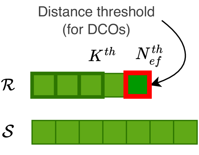
((a)) HNSW+

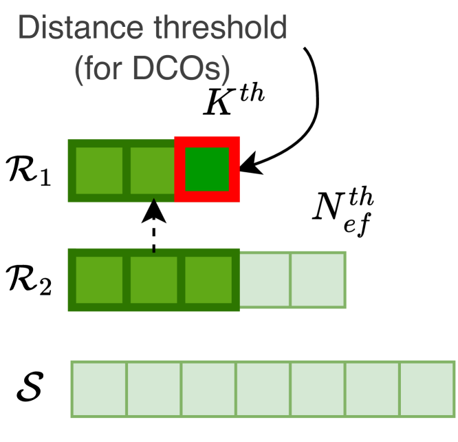
((b)) HNSW++

Figure 3. HNSW+ v.s. HNSW++

Theoretical Analysis. We note that different from HNSW+, which would return the same results as HNSW with high probability, HNSW++ does not aim to return the same results as HNSW (though in practice, it returns nearly the same results as verified in Section 6.2.2). Specifically, HNSW++ would generate a set of candidates, which might be different from that of HNSW+ or HNSW. Among the generated candidates, HNSW++ guarantees to return their KNNs with high probability because it still maintains KNNs with ADSampling, and its guarantee is the same as the one in Corollary 4.2.

HNSW++ v.s. HNSW+. Compared with HNSW+, HNSW++ is expected to have a better time-accuracy trade-off, which we explain as follows. First, consider the time cost. In HNSW++, for each DCO, the threshold distance is the $K^{th}$ largest distance, which is smaller than that used in HNSW+ (i.e., the $N_{ef}^{th}$ largest distance). Correspondingly, in HNSW++, the $\alpha$ value, which is defined as $(dis-r)/r$, is larger than that in HNSW+. Therefore, the time cost for this DCO would be smaller than that in HNSW+ according to the time complexity analysis of ADSampling in Section 3.3. Second, consider the effectiveness. While HNSW++ and HNSW+ use different distances for generating the candidates, we expect that they would generate candidates with similar qualities given that (1) the distances used by the two algorithms should be close (or the same in some cases) and (2) the method used for generating candidates, i.e., greedy beam-search, has a heuristic nature and there is no strong clue that it favors exact distances over approximate ones.

Remarks. We note that the technique of HNSW++ can also be used in other graph-based methods (Malkov and Yashunin, 2020; Li et al., 2019; Fu et al., 2019; Jayaram Subramanya et al., 2019; Malkov et al., 2014). This is because these algorithms also apply the greedy beam search based on a set $\mathcal{R}$ in the query phase.

5.2. IVF++: Towards Cache Friendliness

In the original IVF algorithm, the vectors in the same cluster are stored sequentially. When evaluating their distances, the algorithm scans all the dimensions of these vectors sequentially, which exhibits strong locality of reference, and thus it is cache-friendly. Figure 4(a) illustrates the corresponding data layout (as indicated by the arrow) and the data needed (as indicated by the colored background). In IVF+, though it scans fewer dimensions than IVF, it would not be cache-friendly with the same data layout. Specifically, when IVF+ terminates the dimension sampling process for a data vector, the subsequent dimensions would probably have been loaded into cache from main memory though they are not needed. Figure 4(b) illustrates the corresponding data layout and data needed.

We propose to re-organize the data layout of the candidates and adjust the order of the dimensions of the candidates to be fed to ADSampling accordingly so as to achieve more cache-friendly data accesses. Recall that for each candidate, ADSampling would definitely sample a few, say $d_{1}$, dimensions of the candidate first and then incrementally sample more dimensions depending on the hypothesis testing outcomes. That is, the first $d_{1}$ dimensions of each candidate would be accessed for sure. Motivated by this, we store the first $d_{1}$ dimensions of all candidates sequentially in an array $A_{1}$ and the remaining $D-d_{1}$ dimensions of all candidates sequentially in another array $A_{2}$. We note that the process of re-organizing the data layout can be conducted during the index phase. During the query phase, when using ADSampling for DCOs on the candidates, we follow the following order of the dimensions of the candidates: the first $d_{1}$ dimensions of the first candidate, the first $d_{1}$ dimensions of the second candidate, …, the first $d_{1}$ dimensions of the last candidate, the $D-d_{1}$ dimensions of the first candidate, …, the $D-d_{1}$ dimensions of the last candidate. Figure 4(c) illustrates the corresponding data layout and data needed. We call the resulting algorithm IVF++. IVF++ and IVF+ would produce exactly the same results, but the former is more cache friendly since it utilizes the locality of reference for the first $d_{1}$ dimensions of all candidates.

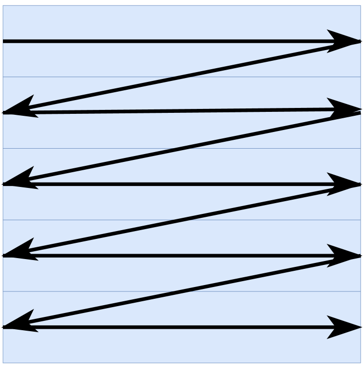
((a)) IVF

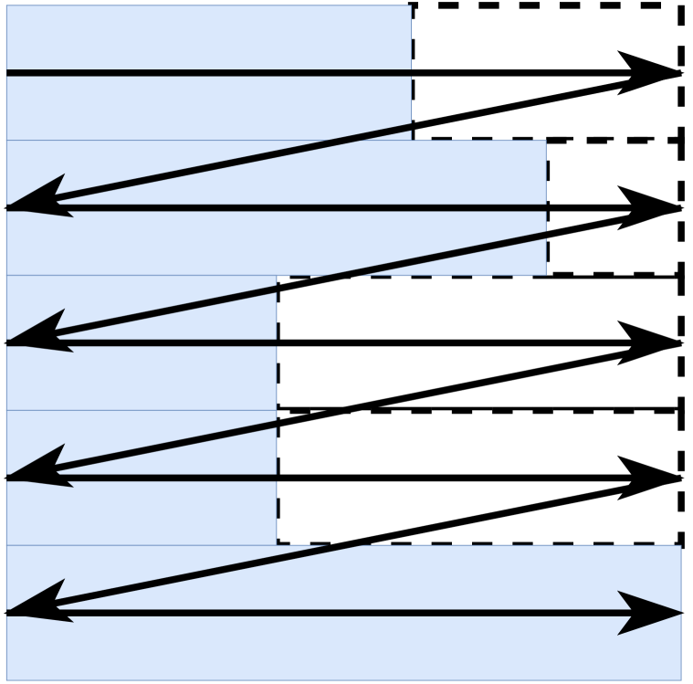
((b)) IVF+

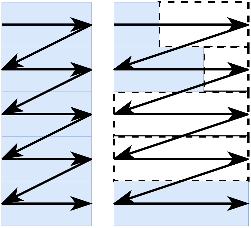
((c)) IVF++

Figure 4. Data Layout and Data Needed

Theoretical Analysis. Since IVF++ and IVF+ differ only in data layout, they have the same theoretical guarantee (Corollary 4.2).

Remarks. We note that the technique used for improving IVF+ with cache friendliness can also be used for improving some other AKNN+ algorithms, including those of tree-based methods (Muja and Lowe, 2014; Dasgupta and Freund, 2008; Ram and Sinha, 2019; Beygelzimer et al., 2006), quantization-based methods (Jegou et al., 2010; Babenko and Lempitsky, 2015) and hashing-based methods (Datar et al., 2004; Gan et al., 2012; Dong et al., 2020). This is because all these algorithms generate the candidates in a batch and then re-rank the candidates for finding out KNNs.

6. Experiment

6.1. Experimental Setup

Datasets. We use six public datasets with varying sizes and dimensionalities , whose details are shown in Table 1. These datasets have been widely used to benchmark AKNN algorithms  (Lu et al., 2021; Li et al., 2020, 2019). We note that these public datasets provide both data and query vectors.

Table 1. Dataset Statistics

Dataset	Size	$D$	Query Size	Data Type
Msong	992,272	420	200	Audio
DEEP	1,000,000	256	1,000	Image
Word2Vec	1,000,000	300	1,000	Text
GIST	1,000,000	960	1,000	Image
GloVe	2,196,017	300	1,000	Text
Tiny5M	5,000,000	384	1,000	Image

Algorithms. For reliable DCOs, we compare our proposed method ADSampling with the conventional FDScanning and PDScanning (Partial Dimension Scanning), which we explain below. PDScanning incrementally scans the dimensions of a raw vector and terminates the process when the distance based on the partially scanned $d$ dimensions, i.e., $\sqrt{\sum_{i=1}^{d}x_{i}^{2}}$, is greater than the distance threshold $r$. We note that PDScanning starts with zero dimensions but not a pre-set number of dimensions since (1) it is hard to set the number and (2) starting from a certain number of dimensions or zero dimensions have very similar performance given the fact that the dimensions are scanned incrementally. We also note that PDScanning is an exact algorithm for DCOs and has the worst-case time complexity of $O(D)$. We name the AKNN algorithms with PDScanning for DCOs as AKNN* and the one with a further optimized data layout as AKNN** (for IVF only). We exclude those distance approximation methods such as product quantization and random projection from comparison since as explained in Section 1 and further verified in Section 6.2.4, they can hardly achieve reliable DCOs. For AKNN algorithms, we mainly focus on HNSW (Malkov and Yashunin, 2020) and IVF (Jegou et al., 2010) for providing the contexts of DCOs since they correspond to two state-of-the-art AKNN algorithms as benchmarked in (Aumüller et al., 2020; Li et al., 2019). We note that these methods are widely adopted in industry (including Faiss (Johnson et al., 2019), Milvus (Wang et al., 2021b) and PASE (Yang et al., 2020)). For better comprehensiveness, we also consider one of the best tree-based methods Annoy (Annoy, 2016) (as benchmarked in (Aumüller et al., 2020; Li et al., 2019)) and a hashing-based method PMLSH (Zheng et al., 2020). We note that their performance of time-accuracy tradeoff is suboptimal compared with HNSW and IVF. Due to the limit of space, we include their results in Appendix B.

Performance Metrics. We use two metrics to measure the accuracy: (1) recall (Aumüller et al., 2020; Li et al., 2019; Malkov and Yashunin, 2020; Jegou et al., 2010), i.e., the ratio between the number of successfully retrieved ground truth KNNs and $K$ and (2) average distance ratio (Patella and Ciaccia, 2009; Gan et al., 2012; Huang et al., 2015; Sun et al., 2014; Patella and Ciaccia, 2008), i.e., the average of the distance ratios (which equals to the average relative error on distance plus one) of the retrieved $K$ objects wrt the ground truth KNNs. We adopt the query-per-second (QPS), i.e., the number of handled queries per second, to measure efficiency. Note that the query time is measured end-to-end (i.e., including the time of random transformation on query vectors). We decompose the time cost in Section 6.2.3. We also measure the total number of dimensions evaluated by an algorithm. For AKNN algorithms, it means the total number of dimensions of the candidates (since for each candidate, all of its dimensions are used for computing its distance). For AKNN+ (AKNN*) and AKNN++ (AKNN**) algorithms, it means the total number of sampled (scanned) dimensions of the candidates (since for a candidate, only those sampled (scanned) dimensions are used for computing its distance approximately). All the mentioned metrics are averaged over the whole query set.

Implementation. The implementation of an AKNN algorithm consists of two phases. During the index phase, we first generate a random orthogonal transformation matrix with the NumPy library, store it and apply the transformation to all data vectors. Then we feed the transformed vectors (the raw vectors for AKNN, AKNN* and AKNN**) into existing AKNN algorithms. In particular, for HNSW, HNSW+, HNSW++ and HNSW* (note that they have the same graph structure), our implementation is based on hnswlib (Malkov and Yashunin, 2020), while for IVF, IVF+, IVF++, IVF* and IVF** (note that they have the same cluster structure), our implementation of K-means clustering is based on the Faiss library (Johnson et al., 2019). Then during the query phase, all algorithms are implemented in C++. For a new query, we first transform the query vector with the Eigen library (Guennebaud et al., 2010) for fast matrix multiplication when running AKNN+ and AKNN++ algorithms (For AKNN, AKNN* and AKNN**, they involve no transformation). Then we feed the vector into the AKNN, AKNN+, AKNN++, AKNN* and AKNN** algorithms. Following (Wang et al., 2021a; Li et al., 2019), we disable all hardware-specific optimizations including SIMD, memory prefetching and multi-threading (including those in the Eigen library) so as to focus on the comparison among algorithms themselves.

Parameter Setting. For HNSW, two parameters are preset to control the construction of the graph, namely $M$ to control the number of connected neighbors and $efConstruction$ to control the quality of approximate nearest neighbors. We follow the parameter settings of its original work (Malkov and Yashunin, 2020) where the parameters are set as $M=16$ and $efConstruction=500$. For IVF, as suggested in the Faiss library , the number of clusters should be around the square root of the cardinality of the database. Since we focus on million-scale datasets, it’s set to be 4,096. For ADSampling, we vary $\epsilon_{0}$ with values of 1.5, 1.8, 2.1, 2.4, 2.7 and 3.0 and study its effects in Section 6.2.5. Based on the results, we adopt the setting of $\epsilon_{0}=2.1$ as the default one. Recall that in ADSampling, it incrementally samples some dimensions of a data vector and performs a hypothesis testing in iterations. To avoid the overhead of frequent hypothesis testings, we sample $\Delta_{d}$ dimensions at each iteration. By default, we set $\Delta_{d}=32$. Its parameter study is also provided in Section 6.2.5.

All C++ source codes are complied by g++ 9.4.0 with -O3 optimization under Ubuntu 20.04LTS. The Python source codes (which are used during the index phase) are run on Python 3.8. All experiments are conducted on a machine with AMD Threadripper PRO 3955WX 3.9GHz 16C/32T processor and 64GB RAM. The code and datasets are available at https://github.com/gaoj0017/ADSampling.

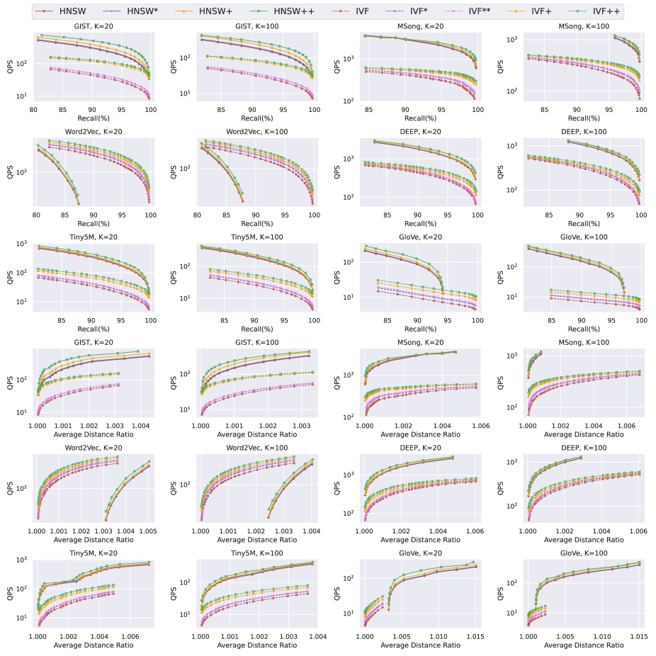
Figure 5. Time-Accuracy Tradeoff (HNSW and IVF).

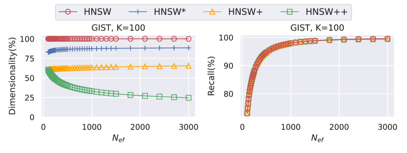
((a)) HNSW

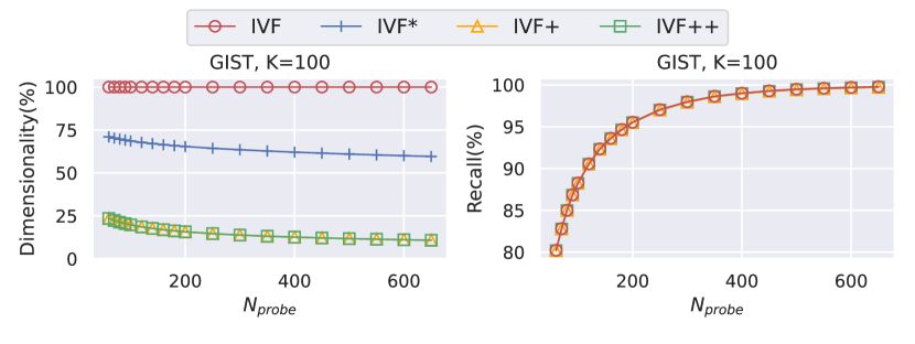
((b)) IVF

Figure 6. Evaluated Dimensionality and Accuracy.

6.2. Experimental Results

6.2.1. Overall Results (Time-Accuracy Trade-Off)

We plot the QPS-recall curve (upper panels, upper-right is better) and the QPS-ratio curve (lower panels, upper-left is better) by varying $N_{ef}$ for HNSW/HNSW*/HNSW+/HNSW++ and $N_{probe}$ for IVF/IVF*/IVF**/IVF+/IVF++ in Figure 5. We focus only on the region with the recall at least 80% based on practical needs. Overall, with the results in Figure 5, we can observe clearly that (1) the AKNN+ algorithms (represented by the orange curves) outperform the plain AKNN algorithms (represented by the red curves), (2) the AKNN++ algorithms (represented by the green curves) further outperform the AKNN+ algorithms, (3) the baseline method HNSW* (represented by the blue curves) brings very minor improvements on HNSW for all the tested datasets and (4) the baseline methods IVF* (represented by the blue curves) and IVF** (represented by the violet curves) are outperformed by IVF+ consistently and significantly (and by IVF++ with an even larger margin).

Besides, we have the following observations. (1) Our techniques bring more improvements on IVF than on HNSW (even when IVF performs better than HNSW, e.g., on Word2Vec). We ascribe it to the fact that other computations than DCOs of HNSW are heavier than those of IVF (as shown in Figure 2). (2) Our techniques in general bring more improvements on high accuracy region than on low accuracy region (e.g., GIST 95% v.s. 85%). This is because when an AKNN algorithm targets higher accuracy, it unavoidably generates more low-quality candidates with larger distance gap $\alpha$, for which it needs fewer dimensions for reliable DCOs. (3) The data layout optimization brings more improvements on IVF+ (i.e., IVF++ v.s. IVF+) than on IVF* (i.e., IVF** v.s. IVF*). This is because ADSampling has the logarithmic complexity while the baseline PDScanning has the linear complexity. Specifically, the first $\Delta_{d}$ dimensions are sufficient for many DCOs when using ADSampling and thus, many accesses to the second array $A_{2}$ in Figure 4(c) can be avoided. When using PDScanning for the DCOs, it will still access the second array frequently because it needs more than $\Delta_{d}$ dimensions.

6.2.2. Results of Evaluated Dimensions and Recall

We then study the number of evaluated dimensions and the recall of AKNN/AKNN+/AKNN++/AKNN* (AKNN** has exactly the same curve as AKNN* and thus, is omitted) under the same search parameter setting ($N_{ef}$ for HNSW and $N_{probe}$ for IVF). For the number of evaluated dimensions, we measure its ratio over that of AKNN in percentage for the ease of comparison. The results are shown in Figure 6.

Overall Results. In Figure 6, we can observe clearly that AKNN+ and AKNN++ evaluate much fewer dimensions than AKNN while reaching nearly the same recall. Specifically, on GIST, for all tested values of $N_{ef}$, the accuracy loss of HNSW+ and HNSW++ (compared with HNSW) is no more than 0.14% and that of IVF+ and IVF++ is no more than 0.1%. At the same time, HNSW++ saves from 39.4% to 75.3% of the total dimensions, HNSW+ saves from 34.5% to 39.4% and IVF+/IVF++ save from 76.5% to 89.2%. The baseline method HNSW* saves from 10.9% to 15.7%, which explains its minor improvement on HNSW. IVF*/IVF** saves from 28.9% to 40.4%.

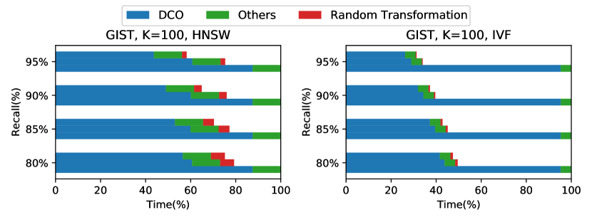
Figure 7. Decomposition of Time Cost (At a particular recall, the three horizontal bars from top to bottom, represent the AKNN++, AKNN+ and AKNN algorithms, respectively. The time cost is normalized by the cost of the original AKNN algorithms).

HNSW+ v.s. HNSW++. We further compare HNSW+ and HNSW++. According to Figure 6(a), we have the following observations. (1) HNSW++ evaluates fewer dimensions than HNSW+, which largely explains the result that HNSW++ runs faster than HNSW+. (2) HNSW++ reaches nearly the same recall as HNSW+, which empirically shows that using approximate distances for graph routing has nearly the same effectiveness as using exact distances. (3) The evaluated dimensions (its ratio over those of HNSW in percentage) of HNSW+ increases wrt $N_{ef}$ while those of HNSW++ decreases wrt $N_{ef}$. This is because HNSW+ conducts DCOs with the $N_{ef}^{th}$ NN’s distance as the threshold, whose distance increases wrt $N_{ef}$, and thus a larger $N_{ef}$ leads to smaller distance gap $\alpha$, which entails more dimensions for a reliable DCO. For HNSW++, as mentioned in 6.2.1, when targeting high recall, an AKNN algorithm inevitably generates many low-quality candidates with larger $\alpha$’s, and thus, it needs fewer dimensions for DCOs.

IVF+ v.s. IVF++. IVF+ and IVF++ differ only in data layout, and thus they have exactly the same accuracy and evaluated dimensions.

6.2.3. Results of Time Cost Decomposition

We note that applying ADSampling entails the extra cost of randomly transforming the data and query vectors. In particular, the cost of transforming the data vectors lies in the index phase and can be amortized by all the subsequent queries on the same database. The transformation of the query vectors is conducted during the query phase when a query comes and its cost can be amortized by all the DCOs involved for answering the same query. We implement this step (a.k.a, Johnson-Lindenstrauss Transformation (Johnson and Lindenstrauss, 1984; Freksen, 2021)) as a matrix multiplication operation for simplicity, which takes $O(D^{2})$ time. We note that this step can be performed in less time with advanced algorithms (Freksen, 2021), e.g., it takes $O(D\log D)$ time with Kac’s Walk (Jain et al., 2022). We show the results of time cost decomposition on the dataset GIST. It has the highest dimensionality and correspondingly the largest overhead for random transformation. We decompose the time cost in Figure 7. We note that the cost of random transformation for HNSW+/HNSW++ takes at most 6.18% of the total cost of the original HNSW. As the accuracy increases, the percentage decreases (e.g., for 95% recall, it reduces to 2.02%). For IVF+, the percentage is no greater than 1.11%.

6.2.4. Results for Evaluating the Feasibility of Distance Approximation Techniques for Reliable DCOs

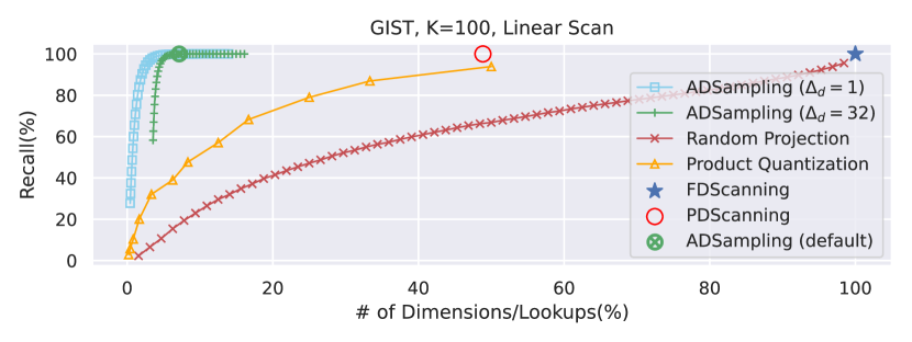
Figure 8. Feasibility for Reliable DCOs (Recall).

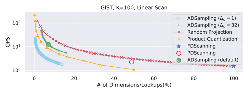
Figure 9. Feasibility for Reliable DCOs (QPS).

We next study the feasibility of two distance approximation methods, including random projection and product quantization (Jegou et al., 2010) (with the typical setting of 256 centroids per partition (Jegou et al., 2010; Wang et al., 2018)), for reliable DCOs. We include the results of ADSampling, PDScanning and FDScanning for comparison. To test the best possible recall a method can reach, we conduct this experiment with an exact KNN algorithm, namely linear scan. Specifically, for random projection and product quantization, we scan all the data objects and return the K objects with the minimum approximate distances. For ADSampling and PDScanning, like IVF, we maintain a KNN set and conduct DCOs for each object sequentially. We plot the recall-number of dimensions/lookups   curves in Figure 8. For random projection, we vary the dimensionality of the projected vectors and observe that (1) it introduces 3.71% accuracy loss while reducing only 1.04% dimensions (2) when reducing half of the dimensionality, its recall is no more than 70%. For product quantization, we vary its quantization code size (i.e., the number of partitions) and observe that in the best possible case (i.e., the case of encoding every two dimensions with one code), it still introduces 6.2% accuracy loss. Therefore, neither product quantization nor random projection can achieve reliable DCOs with remarkably better efficiency than FDScanning.

For ADSampling, we test two settings $\Delta_{d}=1$ and $\Delta_{d}=32$. The former represents the best possible recall-dimension tradeoff of our method and the latter represents a practical setting with less frequent hypothesis testing (i.e., our default setting). We plot their curves by varying $\epsilon_{0}$ from 0.0 to 4.0. We observe that for $\Delta_{d}=1$, it samples 6.61% of the total dimensions while reaching ¿99.9% recall and for $\Delta_{d}=32$, it samples 7.11% of the total dimensions while reaching ¿ 99.9% recall. Thus, ADSampling achieves much better recall-dimension tradeoff than FDScanning.

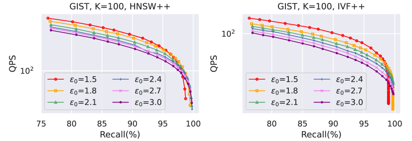
Figure 10. Parameter Study on $\epsilon_{0}$ of AKNN++ Algorithms.

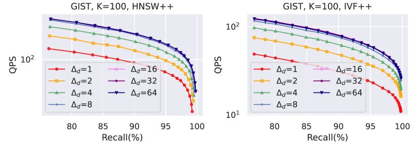
Figure 11. Parameter Study on the $\Delta_{d}$ of AKNN++ Algorithms.

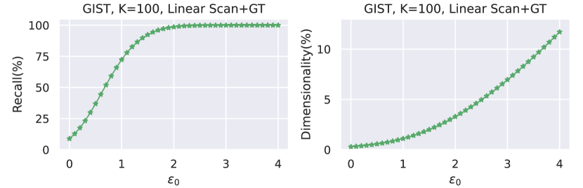
Figure 12. Verification for Theoretical Analysis.

In Figure 9, we plot the QPS-dimensions/lookups curves. We have the following observations. (1) ADSampling (with default setting), which is marked with a green cross within a green circle, has the QPS significantly higher than FDScanning and PDScanning. This is because it exploits only 7.11% of the total dimensions while achieving a recall over $99.9\%$. (2) At the same dimensionality, random projection has its efficiency better than ADSampling. This is because random projection has fixed dimensionality and can organize the projected vectors sequentially in an array to achieve better cache-friendliness. However, we note that when random projection has the same QPS as ADSampling (default), its recall does not exceed 40%.

6.2.5. Results of Parameter Study

Parameter $\epsilon_{0}$ is a critical parameter for the ADSampling algorithm since it directly controls the trade-off between the accuracy and the efficiency (recall that a larger $\epsilon_{0}$ means a smaller significance value for the hypothesis testing, which further implies a more accurate result of the hypothesis testing). Figure 10 plots the QPS-recall curves of HNSW++ (left panel) and IVF++ (right panel) with different $\epsilon_{0}$. In general, we observe from the figures that with a larger $\epsilon_{0}$, the QPS-recall curves moves lower right. This is because a larger $\epsilon_{0}$ leads to better accuracy at the cost of efficiency. We observe that when $\epsilon_{0}=2.1$, it introduces little accuracy loss while further increasing $\epsilon_{0}$ would decrease the efficiency. Thus, in order to improve the efficiency without losing much accuracy, we suggest to set $\epsilon_{0}$ around $2.1$. The results for HNSW+ and IVF+ are similar and omitted due to the page limit.

Figure 11 plots the QPS-recall curves of HNSW++ and IVF++ with different $\Delta_{d}$. We observe that too frequent hypothesis testing (e.g., when $\Delta_{d}=1$) would do harm to the performance. It’s worth noting that a small $\Delta_{d}$ implies that it can terminate sampling immediately when enough information is collected, but it would require more arithmetic operations for hypothesis testing. Our empirical study shows that when $\Delta_{d}=16,32,64$, it achieves the best trade-off.

6.2.6. Results for Verifying Theoretical Results

We further empirically verify Lemma 3.2 and  3.3. As a verification study, the experimental setting is different. To eliminate the accuracy loss caused by AKNN algorithms, we conduct the verification study based on linear scan, which itself is an exact KNN algorithm. Note that in KNN query processing, the result of the former DCOs can affect the distance thresholds of the latter DCOs, which introduces some bias into a verification study. To eliminate it, we provide a fixed distance threshold (the exact distance of the ground truth Kth NN) to make the DCOs independent with each other. To test the actual needed dimensionality, we set $\Delta_{d}=1$. With this setting, the recall represents the proportion of successful DCOs for positive objects (recall that those for negative objects will never fail), and thus, it empirically reflects the success probability of a single DCO with ADSampling. The left panel of Figure 12 shows that the failure probability indeed decays following a quadratic-exponential trend and reaches near 100% accuracy around $\epsilon_{0}=2$. The right panel shows that the number of evaluated dimensions increases following a quadratic trend, which is slow when $\epsilon_{0}$ is small (when $\epsilon_{0}=2$, the total number of evaluated dimensions is around $3\%$ of that of the plain FDScanning).

7. Related Work

Approximate K Nearest Neighbor Search. Existing AKNN algorithms can be categorized into four types: (1) graph-based (Malkov and Yashunin, 2020; Malkov et al., 2014; Li et al., 2019; Fu et al., 2019, 2021; Iwasaki, 2016), (2) quantization-based (Jegou et al., 2010; Ge et al., 2013; Guo et al., 2020; Gong et al., 2013; Babenko and Lempitsky, 2014, 2015), (3) tree-based  (Muja and Lowe, 2014; Dasgupta and Freund, 2008; Ram and Sinha, 2019; Beygelzimer et al., 2006; Ciaccia et al., 1997) and (4) hashing-based (Indyk and Motwani, 1998; Datar et al., 2004; Gan et al., 2012; Tao et al., 2010; Huang et al., 2015; Sun et al., 2014; Lu et al., 2020; Zheng et al., 2020; Li et al., 2018). In particular, graph-based methods show superior performance for in-memory AKNN query. Quantization-based methods are powerful when memory is limited. Hashing-based methods provide rigorous theoretical guarantee. We refer readers to recent tutorials (Echihabi et al., 2021; Qin et al., 2021), reviews and benchmarks (Li et al., 2019; Aumüller et al., 2020; Boytsov and Naidan, 2013; Patella and Ciaccia, 2009; Wang et al., 2021a) for details. There are also plentiful studies, which apply machine learning (ML) to accelerate AKNN (Baranchuk et al., 2019; Feng et al., 2022; Li et al., 2020; Dong et al., 2020). (Baranchuk et al., 2019; Feng et al., 2022) apply reinforcement learning in graph routing which substitutes greedy beam search. (Li et al., 2020) learns to early terminate searching. (Dong et al., 2020) uses ML to construct an index structure. Note that all above methods apply ML for candidate generation. These ML-based methods are orthogonal to our techniques and our techniques can help them with finding KNNs among the generated candidates.

Random Projection for AKNN. While random projection can hardly be used for reliable DCOs during the phase of re-ranking candidates of KNNs as explained and verified earlier, it has been widely applied in LSH (Indyk and Motwani, 1998; Datar et al., 2004; Gan et al., 2012; Tao et al., 2010; Sun et al., 2014; Huang et al., 2015; Lu et al., 2020) and random partition/projection tree (Ram and Sinha, 2019; Dasgupta and Freund, 2008) during the phase of generating candidates of KNNs. Our study differs from these studies in (1) we project different objects to vectors with different dimensions flexibly while these studies project all objects to vectors with equal dimensions; (2) we set the number of dimensions of a projected vector for an object automatically based on its DCO via hypothesis testing while these studies need to set the number with manual efforts; and (3) we use the projected vectors (in DCOs) during the phase of finding out KNNs from the generated candidates while these studies use the projected vectors during the phase of generating candidates. Therefore, these studies are orthogonal to our study.

Dimension Sampling for AKNN. We notice that a MAB (multi-armed bandit)-oriented approach (LeJeune et al., 2019) also applies dimension sampling and claims logarithmic complexity. Our study is different from (LeJeune et al., 2019) in the following aspects. Problem-wise, (LeJeune et al., 2019) targets the AKNN problem itself and aims to find a superset of the set containing the KNNs. It is non-trivial to adapt (LeJeune et al., 2019) to DCOs (the focus of our paper). Theory-wise, (LeJeune et al., 2019)’s logarithmic complexity relies on some strong assumptions on the data (which may not hold in practice) while ours relies on no assumptions. Technique-wise, (1) (LeJeune et al., 2019) samples the original vectors directly while ours first randomly transforms the vectors and then samples the transformed vectors. Our way has the advantage that the error bound of an approximate distance is based on the concentration inequality of random projection and does not rely on any assumptions as (LeJeune et al., 2019) does; and (2) (LeJeune et al., 2019) uses some lower/upper bounds to determine the number of sampled dimensions while ours uses sequential hypothesis testing. Our way has no false positives while (LeJeune et al., 2019) has both false positives and false negatives. In summary, (LeJeune et al., 2019) and our work only share a high-level idea of dimension sampling and differ in many aspects including problem, theory and technique.

8. Conclusion and Discussion

We identify the distance comparison operation which dominates the time cost of nearly all AKNN algorithms and demonstrate opportunities to improve its efficiency. We propose a new randomized algorithm for the DCO which runs in logarithmic time wrt $D$ in most cases and succeeds with high probability. Based on it, we further develop one generic and two algorithm-specific techniques for AKNN algorithms. Our experiments show that the enhanced AKNN algorithms outperform the original ones consistently. We also provide rigorous theoretical analysis for all our techniques.

We would like to highlight the following extensions and applications of our techniques. (1) Our techniques can be trivially extended to two other widely-adopted similarity metrics, namely cosine similarity and inner product, via simple transformation. Specifically, the cosine-based similarity search on some given data and query vectors is equivalent to the Euclidean nearest neighbor search on their normalized data and query vectors where ADSampling is applicable. The inner product comparison of whether $\left<\mathbf{o},\mathbf{q}\right>\geq r$ can be reduced to the DCO of whether $\left\|\mathbf{o}/\|\mathbf{o}\|-\mathbf{q}/\|\mathbf{q}\|\right\|\leq\sqrt{2-2r/(\|\mathbf{o}\|\cdot\|\mathbf{q}\|)}$, where the distance threshold equals to $\sqrt{2-2r/(\|\mathbf{o}\|\cdot\|\mathbf{q}\|)}$ . (2) DCOs are also ubiquitous in many other tasks of high-dimensional data management and analysis such as clustering (Lloyd, 1982) and outlier detection (Bay and Schwabacher, 2003). Our techniques have the potential to accelerate existing methods for those tasks by reducing the cost of DCOs while keeping the accuracy.

9. Acknowledgements

This research is supported by the Ministry of Education, Singapore, under its Academic Research Fund (Tier 2 Awards MOE-T2EP20220-0011 and MOE-T2EP20221-0013). Any opinions, findings and conclusions or recommendations expressed in this material are those of the author(s) and do not reflect the views of the Ministry of Education, Singapore. We would like to thank Yi Li (SPMS, NTU) for answering many questions about high-dimensional probability and the anonymous reviewers for providing constructive feedback and valuable suggestions.

appendix

Appendix A Theoretical Analysis

In this section, we prove Lemma 3.3 in detail. We assume that we sample one additional dimension of $\mathbf{y}$ each time. Let $\gamma(d)=(1+\epsilon_{0}/\sqrt{d})$. We have

(13) $$\mathbb{E}\left[\hat{D}\right]= \sum_{d=1}^{D}d\cdot\mathbb{P}\left\{\hat{D}=d\right\}=\sum_{d=1}^{D}\mathbb{P}\left\{\hat{D}\geq d\right\}$$

(14) $$= \sum_{d=1}^{D}\mathbb{P}\left\{\forall p<d,\sqrt{\frac{D}{p}}\|\mathbf{y}|_{1,2,...,p}\|\leq\gamma(p)\cdot r\right\}$$

(15) $$= \sum_{d=1}^{D}\mathbb{P}\left\{\forall p<d,\sqrt{\frac{D}{p}}\|\mathbf{y}|_{1,2,...,p}\|\leq\gamma(p)\cdot\frac{\|\mathbf{y}\|}{1+\alpha}\right\}$$

(16) $$\leq 1+\sum_{d=1}^{D-1}\mathbb{P}\left\{\sqrt{\frac{D}{d}}\|\mathbf{y}|_{1,2,...,d}\|\leq\gamma(d)\cdot\frac{\|\mathbf{y}\|}{1+\alpha}\right\}$$

where (14) is because $\hat{D}\geq d$ represents the event that all the previous hypothesis testings cannot reject the hypothesis and (16) relaxes the event corresponding to all the testings (i.e., $\forall p<d$) to that corresponding to the last testing (i.e., $p=d-1$).

We denote $\tilde{d}:=\epsilon_{0}^{2}/\alpha^{2},d_{0}:=\mathrm{ceil}(\tilde{d})$ and relax the probability for $d\leq d_{0}$ to $1$:

(17) $$\mathbb{E}\left[\hat{D}\right]\leq 1+d_{0}+\sum_{d=d_{0}+1}^{D}\mathbb{P}\left\{\sqrt{\frac{D}{d}}\|\mathbf{y}|_{1,2,...,d}\|\leq\frac{\gamma(d)}{1+\alpha}\|\mathbf{y}\|\right\}$$

Let’s focus on the last term of (17) and deduce from it as follows,

(18) $$\sum_{d=d_{0}+1}^{D}\mathbb{P}\left\{\sqrt{\frac{D}{d}}\|\mathbf{y}|_{1,2,...,d}\|\leq\frac{\gamma(d)}{1+\alpha}\|\mathbf{y}\|\right\}$$

(19) $$= \sum_{d=d_{0}+1}^{D}\mathbb{P}\left\{\sqrt{\frac{D}{d}}\|\mathbf{y}|_{1,2,...,d}\|\leq\left[1-\left(1-\frac{\gamma(d)}{1+\alpha}\right)\right]\|\mathbf{y}\|\right\}$$

(20) $$\leq \sum_{d=d_{0}+1}^{D}\exp\left[-c_{0}d\left(1-\frac{\gamma(d)}{1+\alpha}\right)^{2}\right]$$

(21) $$= \sum_{d=d_{0}+1}^{D}\exp\left[-\frac{c_{0}\alpha^{2}}{(1+\alpha)^{2}}\left(\sqrt{d}-\sqrt{\tilde{d}}\right)^{2}\right]$$

(22) $$\leq \int_{d_{0}}^{D}\exp\left[-\frac{c_{0}\alpha^{2}}{(1+\alpha)^{2}}\left(\sqrt{x}-\sqrt{\tilde{d}}\right)^{2}\right]\mathrm{d}x$$

(23) $$= \int_{d_{0}}^{D}\exp\left[-\frac{c_{0}\epsilon_{0}^{2}}{(1+\alpha)^{2}}\left(\sqrt{\frac{x}{\tilde{d}}}-1\right)^{2}\right]\mathrm{d}x$$

(24) $$= \tilde{d}\int_{d_{0}/\tilde{d}}^{D/\tilde{d}}\exp\left[-\frac{c_{0}\epsilon_{0}^{2}}{(1+\alpha)^{2}}\left(\sqrt{u}-1\right)^{2}\right]\mathrm{d}u$$

(25) $$\leq \tilde{d}\int_{1}^{+\infty}\exp\left[-\frac{c_{0}\epsilon_{0}^{2}}{(1+\alpha)^{2}}\left(\sqrt{u}-1\right)^{2}\right]\mathrm{d}u$$

where (19) rewrites it to fit the format of Lemma 3.1, (20) applies Lemma 3.1, (21) plugs in $\gamma(d)$, (22) relaxes (21) to an integration, (24) substitutes $u=x/\tilde{d}$, and (25) relaxes the integration to $[1,+\infty)$. Next we first analyze the case of $\alpha\leq\epsilon_{0}$ as follows.

(26) $$\text{(\ref{reduction:relaxing to inf})}\leq \tilde{d}\int_{1}^{+\infty}\exp\left[-\frac{c_{0}\epsilon_{0}^{2}}{(1+\epsilon_{0})^{2}}\left(\sqrt{u}-1\right)^{2}\right]\mathrm{d}u$$

(27) $$\leq \tilde{d}\int_{1}^{+\infty}\exp\left[-\frac{c_{0}}{4}\left(\sqrt{u}-1\right)^{2}\right]\mathrm{d}u$$

where (26) is because $\alpha\leq\epsilon_{0}$ and (27) is yielded when setting $\epsilon_{0}\geq 1$ for reasonable accuracy. Note that the integration is convergent so as to be bounded by a constant. For the case of $\alpha\leq\epsilon_{0}$, we have

(28) $$\mathbb{E}\left[\hat{D}\right]=1+d_{0}+O(\tilde{d})=O(\tilde{d})=O\left(\alpha^{-2}\cdot\epsilon_{0}^{2}\right)$$

For the case of $\alpha>\epsilon_{0}$, its expected dimensionality must be no greater than the case of $\alpha=\epsilon_{0}$ because its distance gap $\alpha$ is larger. Thus, its expected dimensionality is upper bounded by $O(1)$.

Appendix B Results of Tree-based and Hashing-based Methods

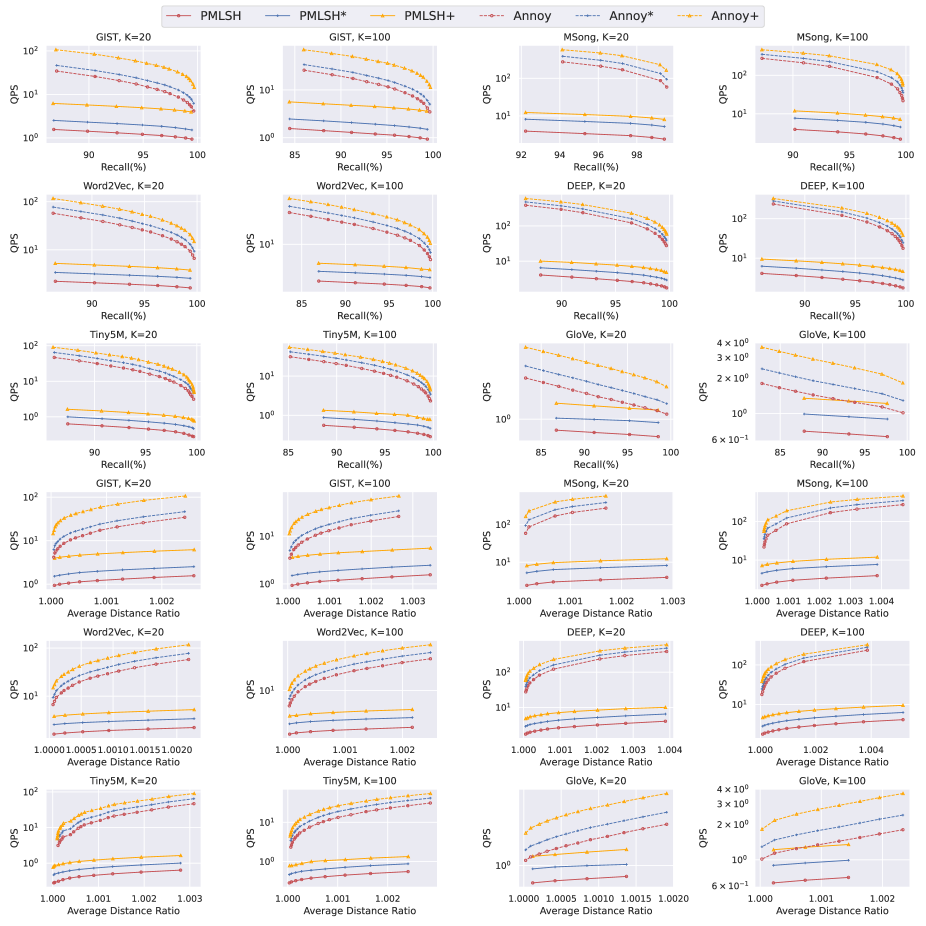
Figure 13. Time-Accuracy Tradeoff (PMLSH and Annoy).

For Annoy, following (Li et al., 2019), we set the number of trees $N_{tree}=50$. During the index phase, we feed the raw data vectors into the indexing algorithm of Annoy (note that Annoy, Annoy+ and Annoy* have the same index structure). Then during the query phase, for Annoy/Annoy*, we load the index and the raw data vectors into main memory, generate candidates by feeding the raw query vector into the the query algorithm of Annoy and re-rank the candidates with FDScanning/PDScanning. For Annoy+, we load the index and the transformed data vectors into main memory, generate candidates by feeding the raw query vector into the the query algorithm of Annoy and re-rank the candidates with ADSampling. For PMLSH, following (Zheng et al., 2020), we set the dimensionality of random projection as 15, the size of internal and leaf nodes of the PM-Tree as 16. Similar to Annoy, during the index phase, we build the indexes based on the raw data vectors. During the query phase, we generate candidates by feeding the raw query vectors to the search algorithm of PMLSH and re-rank them with FDScanning, PDScanning and ADSampling based on raw vectors, raw vectors and transformed vectors respectively. For both methods, we vary the number of accessed candidates to control the time-accuracy tradeoff. We exclude the optimization of data layout for this experiment since it is not applicable for index ensembles (e.g., tree ensembles of Annoy). We plot the QPS-recall and QPS-average distance ratio curves of the compared algorithms in Figure 13. It shows that AKNN+ outperforms the AKNN* and AKNN algorithms consistently and significantly.

References

- (1)
- Ailon and Chazelle (2009) Nir Ailon and Bernard Chazelle. 2009. The Fast Johnson–Lindenstrauss Transform and Approximate Nearest Neighbors. SIAM J. Comput. 39, 1 (2009), 302–322. https://doi.org/10.1137/060673096 arXiv:https://doi.org/10.1137/060673096
- Annoy (2016) Annoy. 2016. Annoy. https://github.com/spotify/annoy.
- Aumüller et al. (2020) Martin Aumüller, Erik Bernhardsson, and Alexander Faithfull. 2020. ANN-Benchmarks: A Benchmarking Tool for Approximate Nearest Neighbor Algorithms. Inf. Syst. 87, C (jan 2020), 13 pages. https://doi.org/10.1016/j.is.2019.02.006
- Babenko and Lempitsky (2014) Artem Babenko and Victor Lempitsky. 2014. Additive Quantization for Extreme Vector Compression. In 2014 IEEE Conference on Computer Vision and Pattern Recognition. 931–938. https://doi.org/10.1109/CVPR.2014.124
- Babenko and Lempitsky (2015) Artem Babenko and Victor Lempitsky. 2015. The Inverted Multi-Index. IEEE Transactions on Pattern Analysis and Machine Intelligence 37, 6 (2015), 1247–1260. https://doi.org/10.1109/TPAMI.2014.2361319
- Baranchuk et al. (2019) Dmitry Baranchuk, Dmitry Persiyanov, Anton Sinitsin, and Artem Babenko. 2019. Learning to Route in Similarity Graphs. In Proceedings of the 36th International Conference on Machine Learning (Proceedings of Machine Learning Research, Vol. 97), Kamalika Chaudhuri and Ruslan Salakhutdinov (Eds.). PMLR, 475–484. https://proceedings.mlr.press/v97/baranchuk19a.html
- Bay and Schwabacher (2003) Stephen D. Bay and Mark Schwabacher. 2003. Mining Distance-Based Outliers in near Linear Time with Randomization and a Simple Pruning Rule. In Proceedings of the Ninth ACM SIGKDD International Conference on Knowledge Discovery and Data Mining (Washington, D.C.) (KDD ’03). Association for Computing Machinery, New York, NY, USA, 29–38. https://doi.org/10.1145/956750.956758
- Beygelzimer et al. (2006) Alina Beygelzimer, Sham Kakade, and John Langford. 2006. Cover trees for nearest neighbor. In Proceedings of the 23rd international conference on Machine learning. 97–104.
- Boytsov and Naidan (2013) Leonid Boytsov and Bilegsaikhan Naidan. 2013. Engineering Efficient and Effective Non-metric Space Library. In Similarity Search and Applications, Nieves Brisaboa, Oscar Pedreira, and Pavel Zezula (Eds.). Springer Berlin Heidelberg, Berlin, Heidelberg, 280–293.
- Chakrabarti and Parthasarathy (2015) Aniket Chakrabarti and Srinivasan Parthasarathy. 2015. Sequential Hypothesis Tests for Adaptive Locality Sensitive Hashing. In Proceedings of the 24th International Conference on World Wide Web (Florence, Italy) (WWW ’15). International World Wide Web Conferences Steering Committee, Republic and Canton of Geneva, CHE, 162–172. https://doi.org/10.1145/2736277.2741665
- Choromanski et al. (2017) Krzysztof M Choromanski, Mark Rowland, and Adrian Weller. 2017. The unreasonable effectiveness of structured random orthogonal embeddings. Advances in neural information processing systems 30 (2017).
- Ciaccia et al. (1997) Paolo Ciaccia, Marco Patella, and Pavel Zezula. 1997. M-Tree: An Efficient Access Method for Similarity Search in Metric Spaces. In Proceedings of the 23rd International Conference on Very Large Data Bases (VLDB ’97). Morgan Kaufmann Publishers Inc., San Francisco, CA, USA, 426–435.
- Cover and Hart (1967) T. Cover and P. Hart. 1967. Nearest neighbor pattern classification. IEEE Transactions on Information Theory 13, 1 (1967), 21–27. https://doi.org/10.1109/TIT.1967.1053964
- Dasgupta and Freund (2008) Sanjoy Dasgupta and Yoav Freund. 2008. Random projection trees and low dimensional manifolds. In Proceedings of the fortieth annual ACM symposium on Theory of computing. 537–546.
- Datar et al. (2004) Mayur Datar, Nicole Immorlica, Piotr Indyk, and Vahab S Mirrokni. 2004. Locality-sensitive hashing scheme based on p-stable distributions. In Proceedings of the twentieth annual symposium on Computational geometry. 253–262.
- Dong et al. (2020) Yihe Dong, Piotr Indyk, Ilya Razenshteyn, and Tal Wagner. 2020. Learning Space Partitions for Nearest Neighbor Search. In International Conference on Learning Representations. https://openreview.net/forum?id=rkenmREFDr
- Echihabi et al. (2021) Karima Echihabi, Kostas Zoumpatianos, and Themis Palpanas. 2021. New Trends in High-D Vector Similarity Search: Al-Driven, Progressive, and Distributed. Proc. VLDB Endow. 14, 12 (jul 2021), 3198–3201. https://doi.org/10.14778/3476311.3476407
- Feng et al. (2022) Chao Feng, Defu Lian, Xiting Wang, Zheng Liu, Xing Xie, and Enhong Chen. 2022. Reinforcement Routing on Proximity Graph for Efficient Recommendation. ACM Trans. Inf. Syst. (jan 2022). https://doi.org/10.1145/3512767 Just Accepted.
- Freksen (2021) Casper Benjamin Freksen. 2021. An Introduction to Johnson-Lindenstrauss Transforms. CoRR abs/2103.00564 (2021). arXiv:2103.00564 https://arxiv.org/abs/2103.00564
- Fu et al. (2021) Cong Fu, Changxu Wang, and Deng Cai. 2021. High dimensional similarity search with satellite system graph: Efficiency, scalability, and unindexed query compatibility. IEEE Transactions on Pattern Analysis and Machine Intelligence (2021).
- Fu et al. (2019) Cong Fu, Chao Xiang, Changxu Wang, and Deng Cai. 2019. Fast Approximate Nearest Neighbor Search with the Navigating Spreading-out Graph. Proc. VLDB Endow. 12, 5 (jan 2019), 461–474. https://doi.org/10.14778/3303753.3303754
- Gan et al. (2012) Junhao Gan, Jianlin Feng, Qiong Fang, and Wilfred Ng. 2012. Locality-Sensitive Hashing Scheme Based on Dynamic Collision Counting. In Proceedings of the 2012 ACM SIGMOD International Conference on Management of Data (Scottsdale, Arizona, USA) (SIGMOD ’12). Association for Computing Machinery, New York, NY, USA, 541–552. https://doi.org/10.1145/2213836.2213898
- Ge et al. (2013) Tiezheng Ge, Kaiming He, Qifa Ke, and Jian Sun. 2013. Optimized product quantization for approximate nearest neighbor search. In Proceedings of the IEEE Conference on Computer Vision and Pattern Recognition. 2946–2953.
- Gong et al. (2013) Yunchao Gong, Svetlana Lazebnik, Albert Gordo, and Florent Perronnin. 2013. Iterative Quantization: A Procrustean Approach to Learning Binary Codes for Large-Scale Image Retrieval. IEEE Transactions on Pattern Analysis and Machine Intelligence 35, 12 (2013), 2916–2929. https://doi.org/10.1109/TPAMI.2012.193
- Guennebaud et al. (2010) Gaël Guennebaud, Benoît Jacob, et al. 2010. Eigen v3. http://eigen.tuxfamily.org.
- Guo et al. (2020) Ruiqi Guo, Philip Sun, Erik Lindgren, Quan Geng, David Simcha, Felix Chern, and Sanjiv Kumar. 2020. Accelerating large-scale inference with anisotropic vector quantization. In International Conference on Machine Learning. PMLR, 3887–3896.
- Huang et al. (2015) Qiang Huang, Jianlin Feng, Yikai Zhang, Qiong Fang, and Wilfred Ng. 2015. Query-aware locality-sensitive hashing for approximate nearest neighbor search. Proceedings of the VLDB Endowment 9, 1 (2015), 1–12.
- Indyk and Motwani (1998) Piotr Indyk and Rajeev Motwani. 1998. Approximate nearest neighbors: towards removing the curse of dimensionality. In Proceedings of the thirtieth annual ACM symposium on Theory of computing. 604–613.
- Iwasaki (2016) Masajiro Iwasaki. 2016. Pruned Bi-directed K-nearest Neighbor Graph for Proximity Search. In Similarity Search and Applications, Laurent Amsaleg, Michael E. Houle, and Erich Schubert (Eds.). Springer International Publishing, Cham, 20–33.
- Jain et al. (2022) Vishesh Jain, Natesh S. Pillai, Ashwin Sah, Mehtaab Sawhney, and Aaron Smith. 2022. Fast and memory-optimal dimension reduction using Kac’s walk. The Annals of Applied Probability 32, 5 (2022), 4038 – 4064. https://doi.org/10.1214/22-AAP1784
- Jayaram Subramanya et al. (2019) Suhas Jayaram Subramanya, Fnu Devvrit, Harsha Vardhan Simhadri, Ravishankar Krishnawamy, and Rohan Kadekodi. 2019. DiskANN: Fast Accurate Billion-point Nearest Neighbor Search on a Single Node. In Advances in Neural Information Processing Systems, H. Wallach, H. Larochelle, A. Beygelzimer, F. d'Alché-Buc, E. Fox, and R. Garnett (Eds.), Vol. 32. Curran Associates, Inc. https://proceedings.neurips.cc/paper/2019/file/09853c7fb1d3f8ee67a61b6bf4a7f8e6-Paper.pdf
- Jegou et al. (2010) Herve Jegou, Matthijs Douze, and Cordelia Schmid. 2010. Product quantization for nearest neighbor search. IEEE transactions on pattern analysis and machine intelligence 33, 1 (2010), 117–128.
- Johnson et al. (2019) Jeff Johnson, Matthijs Douze, and Hervé Jégou. 2019. Billion-scale similarity search with GPUs. IEEE Transactions on Big Data 7, 3 (2019), 535–547.
- Johnson and Lindenstrauss (1984) William B Johnson and Joram Lindenstrauss. 1984. Extensions of Lipschitz mappings into a Hilbert space 26. Contemporary mathematics 26 (1984), 28.
- Jégou et al. (2010) Hervé Jégou, Matthijs Douze, Cordelia Schmid, and Patrick Pérez. 2010. Aggregating local descriptors into a compact image representation. In 2010 IEEE Computer Society Conference on Computer Vision and Pattern Recognition. 3304–3311. https://doi.org/10.1109/CVPR.2010.5540039
- Kane and Nelson (2014) Daniel M. Kane and Jelani Nelson. 2014. Sparser Johnson-Lindenstrauss Transforms. J. ACM 61, 1, Article 4 (jan 2014), 23 pages. https://doi.org/10.1145/2559902
- LeJeune et al. (2019) Daniel LeJeune, Reinhard Heckel, and Richard Baraniuk. 2019. Adaptive Estimation for Approximate -Nearest-Neighbor Computations. In Proceedings of the Twenty-Second International Conference on Artificial Intelligence and Statistics (Proceedings of Machine Learning Research, Vol. 89), Kamalika Chaudhuri and Masashi Sugiyama (Eds.). PMLR, 3099–3107. https://proceedings.mlr.press/v89/lejeune19a.html
- Li et al. (2020) Conglong Li, Minjia Zhang, David G. Andersen, and Yuxiong He. 2020. Improving Approximate Nearest Neighbor Search through Learned Adaptive Early Termination. In Proceedings of the 2020 ACM SIGMOD International Conference on Management of Data (Portland, OR, USA) (SIGMOD ’20). Association for Computing Machinery, New York, NY, USA, 2539–2554. https://doi.org/10.1145/3318464.3380600
- Li et al. (2018) Jinfeng Li, Xiao Yan, Jian Zhang, An Xu, James Cheng, Jie Liu, Kelvin K. W. Ng, and Ti-chung Cheng. 2018. A General and Efficient Querying Method for Learning to Hash. In Proceedings of the 2018 International Conference on Management of Data (Houston, TX, USA) (SIGMOD ’18). Association for Computing Machinery, New York, NY, USA, 1333–1347. https://doi.org/10.1145/3183713.3183750
- Li et al. (2019) Wen Li, Ying Zhang, Yifang Sun, Wei Wang, Mingjie Li, Wenjie Zhang, and Xuemin Lin. 2019. Approximate nearest neighbor search on high dimensional data—experiments, analyses, and improvement. IEEE Transactions on Knowledge and Data Engineering 32, 8 (2019), 1475–1488.
- Liu et al. (2007) Ying Liu, Dengsheng Zhang, Guojun Lu, and Wei-Ying Ma. 2007. A survey of content-based image retrieval with high-level semantics. Pattern Recognition 40, 1 (2007), 262–282. https://doi.org/10.1016/j.patcog.2006.04.045
- Lloyd (1982) S. Lloyd. 1982. Least squares quantization in PCM. IEEE Transactions on Information Theory 28, 2 (1982), 129–137. https://doi.org/10.1109/TIT.1982.1056489
- Lu et al. (2021) Kejing Lu, Mineichi Kudo, Chuan Xiao, and Yoshiharu Ishikawa. 2021. HVS: Hierarchical Graph Structure Based on Voronoi Diagrams for Solving Approximate Nearest Neighbor Search. Proc. VLDB Endow. 15, 2 (oct 2021), 246–258. https://doi.org/10.14778/3489496.3489506
- Lu et al. (2020) Kejing Lu, Hongya Wang, Wei Wang, and Mineichi Kudo. 2020. VHP: approximate nearest neighbor search via virtual hypersphere partitioning. Proceedings of the VLDB Endowment 13, 9 (2020), 1443–1455.
- Malkov et al. (2014) Yury Malkov, Alexander Ponomarenko, Andrey Logvinov, and Vladimir Krylov. 2014. Approximate nearest neighbor algorithm based on navigable small world graphs. Information Systems 45 (2014), 61–68. https://doi.org/10.1016/j.is.2013.10.006
- Malkov and Yashunin (2020) Yu A. Malkov and D. A. Yashunin. 2020. Efficient and Robust Approximate Nearest Neighbor Search Using Hierarchical Navigable Small World Graphs. IEEE Transactions on Pattern Analysis and Machine Intelligence 42, 4 (2020), 824–836. https://doi.org/10.1109/TPAMI.2018.2889473
- Muja and Lowe (2014) Marius Muja and David G Lowe. 2014. Scalable nearest neighbor algorithms for high dimensional data. IEEE transactions on pattern analysis and machine intelligence 36, 11 (2014), 2227–2240.
- Patella and Ciaccia (2008) Marco Patella and Paolo Ciaccia. 2008. The Many Facets of Approximate Similarity Search. In First International Workshop on Similarity Search and Applications (sisap 2008). 10–21. https://doi.org/10.1109/SISAP.2008.18
- Patella and Ciaccia (2009) Marco Patella and Paolo Ciaccia. 2009. Approximate Similarity Search: A Multi-Faceted Problem. J. of Discrete Algorithms 7, 1 (mar 2009), 36–48. https://doi.org/10.1016/j.jda.2008.09.014
- Qin et al. (2021) Jianbin Qin, Wei Wang, Chuan Xiao, Ying Zhang, and Yaoshu Wang. 2021. High-Dimensional Similarity Query Processing for Data Science. In Proceedings of the 27th ACM SIGKDD Conference on Knowledge Discovery & Data Mining (Virtual Event, Singapore) (KDD ’21). Association for Computing Machinery, New York, NY, USA, 4062–4063. https://doi.org/10.1145/3447548.3470811
- Ram and Sinha (2019) Parikshit Ram and Kaushik Sinha. 2019. Revisiting kd-tree for nearest neighbor search. In Proceedings of the 25th acm sigkdd international conference on knowledge discovery & data mining. 1378–1388.
- Satuluri and Parthasarathy (2011) Venu Satuluri and Srinivasan Parthasarathy. 2011. Bayesian locality sensitive hashing for fast similarity search. arXiv preprint arXiv:1110.1328 (2011).
- Schafer et al. (2007) J. Ben Schafer, Dan Frankowski, Jon Herlocker, and Shilad Sen. 2007. Collaborative Filtering Recommender Systems. Springer Berlin Heidelberg, Berlin, Heidelberg, 291–324. https://doi.org/10.1007/978-3-540-72079-9_9
- Sun et al. (2014) Yifang Sun, Wei Wang, Jianbin Qin, Ying Zhang, and Xuemin Lin. 2014. SRS: solving c-approximate nearest neighbor queries in high dimensional euclidean space with a tiny index. Proceedings of the VLDB Endowment (2014).
- Tao et al. (2010) Yufei Tao, Ke Yi, Cheng Sheng, and Panos Kalnis. 2010. Efficient and accurate nearest neighbor and closest pair search in high-dimensional space. ACM Transactions on Database Systems (TODS) 35, 3 (2010), 1–46.
- Vershynin (2018) Roman Vershynin. 2018. High-Dimensional Probability: An Introduction with Applications in Data Science. Cambridge University Press. https://doi.org/10.1017/9781108231596
- Wang et al. (2016) Jun Wang, Wei Liu, Sanjiv Kumar, and Shih-Fu Chang. 2016. Learning to Hash for Indexing Big Data - A Survey. Proc. IEEE 104, 1 (2016), 34–57. https://doi.org/10.1109/JPROC.2015.2487976
- Wang et al. (2021b) Jianguo Wang, Xiaomeng Yi, Rentong Guo, Hai Jin, Peng Xu, Shengjun Li, Xiangyu Wang, Xiangzhou Guo, Chengming Li, Xiaohai Xu, Kun Yu, Yuxing Yuan, Yinghao Zou, Jiquan Long, Yudong Cai, Zhenxiang Li, Zhifeng Zhang, Yihua Mo, Jun Gu, Ruiyi Jiang, Yi Wei, and Charles Xie. 2021b. Milvus: A Purpose-Built Vector Data Management System. In Proceedings of the 2021 International Conference on Management of Data (Virtual Event, China) (SIGMOD ’21). Association for Computing Machinery, New York, NY, USA, 2614–2627. https://doi.org/10.1145/3448016.3457550
- Wang et al. (2018) Jingdong Wang, Ting Zhang, jingkuan song, Nicu Sebe, and Heng Tao Shen. 2018. A Survey on Learning to Hash. IEEE Transactions on Pattern Analysis and Machine Intelligence 40, 4 (2018), 769–790. https://doi.org/10.1109/TPAMI.2017.2699960
- Wang et al. (2021a) Mengzhao Wang, Xiaoliang Xu, Qiang Yue, and Yuxiang Wang. 2021a. A Comprehensive Survey and Experimental Comparison of Graph-Based Approximate Nearest Neighbor Search. Proc. VLDB Endow. 14, 11 (jul 2021), 1964–1978. https://doi.org/10.14778/3476249.3476255
- Yang et al. (2020) Wen Yang, Tao Li, Gai Fang, and Hong Wei. 2020. PASE: PostgreSQL Ultra-High-Dimensional Approximate Nearest Neighbor Search Extension. In Proceedings of the 2020 ACM SIGMOD International Conference on Management of Data (Portland, OR, USA) (SIGMOD ’20). Association for Computing Machinery, New York, NY, USA, 2241–2253. https://doi.org/10.1145/3318464.3386131
- Zheng et al. (2020) Bolong Zheng, Zhao Xi, Lianggui Weng, Nguyen Quoc Viet Hung, Hang Liu, and Christian S Jensen. 2020. PM-LSH: A fast and accurate LSH framework for high-dimensional approximate NN search. Proceedings of the VLDB Endowment 13, 5 (2020), 643–655.