One-loop beta-functions of
quartic enhanced tensor field theories

Joseph Ben Geloun^a,c,† and Reiko Toriumi^b,‡

^aLaboratoire d’Informatique de Paris Nord UMR CNRS 7030
Université Paris 13, 99, avenue J.-B. Clement, 93430 Villetaneuse, France

^bOkinawa Institute of Science and Technology
1919-1 Tancha, Onna-son, Kunigami-gun, Okinawa, Japan 904-0495

^cInternational Chair in Mathematical Physics and Applications
(ICMPA-UNESCO Chair), University of Abomey-Calavi,
072B.P.50, Cotonou, Rep. of Benin

E-mails: ^†bengeloun@lipn.univ-paris13.fr, ^‡reiko.toriumi@oist.jp

Enhanced tensor field theories (eTFT) have dominant graphs that differ from the melonic diagrams of conventional tensor field theories. They therefore describe pertinent candidates to escape the so-called branched polymer phase, the universal geometry found for tensor models. For generic order $d$ of the tensor field, we compute the perturbative $\beta$-functions at one-loop of two just-renormalizable quartic eTFT coined by $+$ or $\times$, depending on their vertex weights. The models $+$ has two quartic coupling constants $(\lambda,\lambda_{+})$, and two 2-point couplings (mass, $Z_{a}$). Meanwhile, the model $\times$ has two quartic coupling constants $(\lambda,\lambda_{\times})$ and three 2-point couplings (mass, $Z_{a}$, $Z_{2a}$). At all orders, both models have a constant wave function renormalization: $Z=1$ and therefore no anomalous dimension. Despite such peculiar behavior, both models acquire nontrivial radiative corrections for the coupling constants. The RG flow of the model $+$ exhibits a particular asymptotic safety: $\lambda_{+}$ is marginal without corrections thus is a fixed point of arbitrary constant value. All remaining couplings determine relevant directions and get suppressed in the UV. Concerning the model $\times$, $\lambda_{\times}$ is marginal and again a fixed point (arbitrary constant value), $\lambda$, $\mu$ and $Z_{a}$ are all relevant couplings and flow to 0. Meanwhile $Z_{2a}$ is a marginal coupling and becomes a linear function of the time scale. This model can neither be called asymptotically safe or free.

Pacs numbers: 11.10.Gh, 04.60.-m, 02.10.Ox
Key words: Renormalization group, beta-function, tensor models, tensor field theories, quantum gravity

1 Introduction

In the search for a gravitational theory resulting from the random generation of geometries, the most notable success to date restricts to two dimensions [1]. The models at the base of this success are those of the celebrated random matrices. These statistical models generate simplicial complexes of dimension 2 and, therefore, discretized random surfaces. An impressive number of results pertains to these models (KPZ equation, integrable models, string theory, …) [2] [3] [4] [5] [6]. More recently, it has been proven [7] [8] that the continuous limit of such random surfaces provides a fluctuating spherical geometry, the Brownian sphere, endowed with the famous Liouville conformal field. Building on the success of statistical matrix models, models of random tensors [9] [10] generate discrete random geometries in higher dimensions and aim at extending these results to higher dimensions [11] [12] [13] [14]. However, their continuum limit is singular and of (Hausdorff) dimension less than 2 [15]. The generated continuous spaces belong to the so-called universal branched polymer geometry which cannot faithfully describe the geometry of our 4-dimensional space-time.

Let us take a closer look at these tensor models and their universality classes. At large size $N$ of the tensor indices, tensor statistical models are dominated by a class of graphs called melonic diagrams or melons. They mainly contribute to the construction of the continuum limit of tensor models. Melonic diagrams define a subclass of topologically spheres and form a tree structure that characterizes the so-called branched polymer phase [16]. It is a striking feature of several tensor models that such melons dominate universally and can be studied analytically. Nevertheless, in the context of quantum gravity, this class of universal branched polymers is undesirable. We therefore aspire to escape from this branched polymer phase.

In order to improve the critical behavior of tensor models, an interesting idea then emerged: one could adjust the scale $N$, considering coupling constants of non-melonic interactions in such a way that a broader class of graphs, including non-melonic ones, contributes to the critical behavior of tensor models [17]. Thus, making the graphs that were previously suppressed contribute to the large limit $N$ defines the working hypothesis now put forward. We call the models of such a program enhanced tensor models. Note that a model exhibiting a phase transition towards a two-dimensional geometry was found in [17]. Therefore, this already proves that enhanced tensor models produce different universality classes and phases from branched polymers. However, notably, the counterpart of these results in quantum field theory (QFT) still remains a vast territory to explore.

QFT is one of the most successful languages of modern physics. It describes with incredible precision complex systems with an infinity of degrees of freedom via the renormalization group (RG). In a different perspective from statistical models whose degrees of freedom are fixed, QFT characterized by a nontrivial propagator unfolds a model flow from microscopic (ultraviolet) to macroscopic (infrared) scales. We consider this point of view to be relevant for random geometry and quantum gravity. Indeed, if the degrees of freedom or modes of the tensor fields are geometric like spacetime quanta, and if the presence of the nontrivial kinetic term induces a flow from UV to IR governed by a given dynamics, we consider that going towards the infrared, these degrees of freedom could agglomerate and form new degrees of freedom in a way similar to a condensation phenomenon [18] [19] [20] [21] [22]. The fact that some QFT of tensor fields called Tensor Field Theories (TFTs), are asymptotically free, and therefore act like Quantum Chromodynamics, brings one more stone to this building [23] [24].

Studying TFTs requires adopting the powerful renormalization group methods of QFT to extract their critical behavior. The renormalization analysis of a TFT is complex because it is a nonlocal field theory [22] [25] [26] [27] [28] [29]. Additionally, one needs to treat the dimensions of coupling constants carefully in order to analyze their flows [30] [31] [32] [33] [34].

More recently, enhanced tensor field theories (eTFTs) have been introduced as extensions of enhanced tensor models [35] [36]. They are proven renormalizable at all orders of perturbation theory and, for the first time, non-melonic graphs contribute to the renormalization group analysis of the coupling constants. Hence, they are crucial candidates for generating a geometric phase different from that of branched polymers and those of 2D geometries.

In this work, we take further the analysis of [35] and compute the $\beta$-functions of two eTFT models. One model is called $+$ and the second model is labeled by $\times$. They were shown to be perturbatively just-renormalizable, at all orders, for given sets of parameters $(d,D,a,b)$, where $d$ is the tensor field order, $D$ is the background group dimension, $b$ parametrizes the kinetic term $\sim p^{2b}(\phi_{p})^{2}$, and $a$ determines the vertex weight $\sim p^{2a}(\phi_{p})^{4}$. The $\beta$-function of model $+$ is studied for generic order $d\geq 3$ of the tensor field and $(D=1,a=(d-2)/2,b=(d-3/2)/2)$. The second model $\times$ has fixed parameters $(D=1,d=3,a=1/2,b=1)$. Both models show exotic features compared to the ordinary TFT and ordinary scalar $\phi^{4}$ QFT.

Our results are the following:

(1) In both models, the wave function renormalization is constant $Z=1$ and therefore the anomalous dimension is vanishing. Although this hints at a classical behavior, there is still a RG flow; the system of $\beta$-functions is remarkably simple and explicitly integrable at one loop. We give the solutions of all equations in terms of the so-called time scale ($t=\log(k/k_{0})$). Based on the power counting theorem of each model and given the type of corrections that appear, we conjecture that the system of $\beta$-functions of each model can be explicitly solved and the models can be constructed in the way of [37] at all orders of perturbation theory. This is a genuine feature of the present quantum models.

(2) The model $+$ has two quartic couplings, $\lambda$ and $\lambda_{+}$, two 2-point couplings, a mass $\mu$ and another 2-point coupling $Z_{a}$ for a quadratic term $p^{2a}(\phi_{p})^{2}$ (introduced to ensure the renormalizability of the model), and a wave function renormalization $Z$. The asymptotic UV-behaviors of all dimensionless couplings are given by (in loose notation that we will make precise)

$$\lambda_{\Lambda\to\infty}=0$$ (1)

$$\lambda_{+;\Lambda\to\infty}=\theta$$ (2)

$$\mu_{\Lambda\to\infty}=0$$ (3)

$$Z_{a;\Lambda\to\infty}=c\,\theta$$ (4)

$$Z=1$$ (5)

where $\theta$ and $c$ are real constants. The coupling $\lambda_{+}$ is marginal and does not acquire any correction: it is a fixed point. The second quartic coupling $\lambda$ is relevant, still running, tends to blow up in the IR and becomes exponentially suppressed in the UV. The mass and $Z_{a}$ are both relevant operators and get suppressed in the UV. In particular, $Z_{a}$ reaches a constant whereas the mass vanishes. We can call this model asymptotically safe with a free parameter $\lambda_{+}=\theta$ (a line of fixed points) and endowed with 3 relevant directions. However, one notes that $\lambda_{+}$ does not flows to reach a fixed value, it is already set at a constant value. In a sense, this is a new kind of asymptotic safety. Strictly speaking, this model is not asymptotically free as two couplings, namely $\lambda_{+}$ and $Z_{a}$ do not flow to 0, and therefore the Gaussian fixed point is never reached unless $\lambda_{+}$ is set to 0. The model is nearly super-renormalizable because of the number of relevant couplings that flow. However it cannot be stringently super-renormalizable because of the presence of a marginal coupling.

(3) The model $\times$ is endowed with two quartic couplings, $\lambda_{\times}$ and $\lambda$, three 2-point couplings $\mu,Z_{a}$ and $Z_{2a}$, and a wave function renormalization $Z$. The UV-behavior of the dimensionless coupling is delivered by the system (in loose notation again):

$$\lambda_{\Lambda\to\infty}=0$$ (6)

$$\lambda_{\times;\Lambda\to\infty}=\theta$$ (7)

$$\mu_{\Lambda\to\infty}=0$$ (8)

$$Z_{a;\Lambda\to\infty}=0$$ (9)

$$Z_{2a;\Lambda\to\infty}=\lim_{\Lambda\to\infty}(c\,\theta\log{\Lambda}+c^{\prime})=\infty$$ (10)

$$Z=1$$ (11)

where $\theta$, $c$ and $c^{\prime}$ are constants. The coupling $\lambda_{\times}$ is marginal and does not receive corrections. It becomes a fixed point: for any $\lambda_{\times}=\theta$ is a line of fixed points. The second coupling $\lambda$ is relevant: it is suppressed in the UV and flows to 0. So behave the mass $\mu$ and the coupling $Z_{a}$. Introduced to make sense of renormalizability, the last 2-point coupling $Z_{2a}$ is marginal and grows linearly in the time scale. As we never reach the Gaussian fixed point (unless we set $\lambda_{\times}=\theta=0$), this model, because of $\lambda_{+}=\theta\neq 0$, cannot be called asymptotically free. On the other hand, because $Z_{2a}$ runs to infinity, the model cannot be called safe (unless once again $\lambda_{\times}=\theta=0)$. This is again a noteworthy behavior different from conventional QFT and TFT models.

The paper is organized as follows. In section 2, we review the essence of [35] and present two models named model $+$ and model $\times$. In section 3, we compute the $\beta$-functions of the model $+$ at 1-loop and interpret the results. The next section 4 presents the same analysis for the model $\times$. The conclusion in section 5 provides a summary of our work and present some perspectives. In appendix A, we detail the integral approximation techniques that we will use to tackle the spectral sums which appear in the calculation of the $\beta$-functions. In appendices B and C, we illustrate the divergent graphs at second order in perturbation theory to support our different conjectures.

2 Review of the renormalizable enhanced quartic TFT

We review here the main results of [35] introducing a class of quartic eTFTs parametrized by $(D,d,a,b)\in{\mathbbm{N}}\times{\mathbbm{N}}\times{\mathbbm{R}}_{+}\times{\mathbbm{R}}_{+}$. In the following sections, we will specify the 4-tuple dealing only with specific models.

2.1 Enhanced TFT models

Consider a field theory defined by a complex function $\phi:(U(1)^{D})^{\times d}\to{\mathbbm{C}}$. The Fourier transform of this complex field yields a order $d$ complex tensor $\phi_{\bf P}$, with ${\bf P}=(p_{1},p_{2},\dots,p_{d})$ a multi-index. $\bar{\phi}_{\bf P}$ denotes its complex conjugate. Note that in the notation $\phi_{\bf P}$ the indices $p_{s}$ define themselves multi-indices:

$$p_{s}=(p_{s,1},p_{s,2},\dots,p_{s,D})\,,\;\,p_{s,i}\in{\mathbbm{Z}}\,.$$ (12)

A tensor field theory action $S$ is built by a sum of convolutions of the tensors $\phi_{\bf P}$ and $\bar{\phi}_{\bf P}$:

$$S[\bar{\phi},\phi]={\rm Tr}_{2}(\bar{\phi}\cdot{\bf K}\cdot\phi)+\mu\,{\rm Tr}_{2}(\phi^{2})+S^{{\rm{int\,}}}[\bar{\phi},\phi]\,,$$ (13)

(14)

$${\rm Tr}_{2}(\bar{\phi}\cdot{\bf K}\cdot\phi)=\sum_{{\bf P},\,{\bf P}^{\prime}}\bar{\phi}_{{\bf P}}\,{\bf K}({\bf P};{\bf P}^{\prime})\,\phi_{{\bf P}^{\prime}}\,,\qquad{\rm Tr}_{2}(\phi^{2})=\sum_{{\bf P}}\bar{\phi}_{{\bf P}}\phi_{{\bf P}}\,,$$ (15)

and where $S^{{\rm{int\,}}}[\bar{\phi},\phi]$ is another convolution involving, in the case we are focusing on, 4 tensors.

Hence, giving ${\bf K}$ and $S^{{\rm{int\,}}}[\bar{\phi},\phi]$ entirely determines the models. For a real parameter $b\geq 0$, we introduce the class of kernels ${\bf K}={\bf{K}}_{b}({\bf P};{\bf P^{\prime}})={\boldsymbol{\delta}}_{{\bf P};{\bf P^{\prime}}}{\bf P}^{2b}$ where

$${\boldsymbol{\delta}}_{{\bf P};{\bf P^{\prime}}}=\prod_{s=1}^{d}\prod_{i=1}^{D}\delta_{p_{s,i},p^{\prime}_{s,i}}\,,\qquad{\bf P}^{2b}=\sum_{s=1}^{d}|p_{s}|^{2b}\,,\qquad|p_{s}|^{2b}=\sum_{i=1}^{D}|p_{s,i}|^{2b}\,,$$ (16)

where $\delta_{p,q}$ denotes the usual Kronecker symbol on ${\mathbbm{Z}}$. It is clear that ${\bf K}_{b}$ represents a power sum of eigenvalues of $d$ Laplacian operators over the $d$ copies of $U(1)^{D}$ ($b=1$ precisely corresponds to Laplacian eigenvalues on the torus). Seeking renormalizable theories [35], more freedom for $b$ values, allowing even values different from integers, leads to interesting models. In ordinary quantum field theory (QFT), the restriction $b\leq 1$ ensures the Osterwalder-Schrader (OS) positivity axiom [37, 38]. In any case, $b$ will be set as a strictly positive real parameter with no other restriction.

We concentrate on the interaction part. Given a parameter $a\geq 0$, we distinguish the following quartic interactions:

$${\rm Tr}_{4;1}(\phi^{4})=\sum_{p_{s},p^{\prime}_{s}\in{\mathbbm{Z}}^{D}}\phi_{12\dots d}\,\bar{\phi}_{1^{\prime}23\dots d}\,\phi_{1^{\prime}2^{\prime}3^{\prime}\dots d^{\prime}}\,\bar{\phi}_{12^{\prime}3^{\prime}\dots d^{\prime}}\,,$$ (17)

$${\rm Tr}_{4;1}([p^{2a}+p^{\prime 2a}]\,\phi^{4})=\sum_{p_{s},p^{\prime}_{s}\in{\mathbbm{Z}}^{D}}\Big{(}|p_{1}|^{2a}+|{p^{\prime}}_{1}|^{2a}\Big{)}\phi_{12\dots d}\,\bar{\phi}_{1^{\prime}23\dots d}\,\phi_{1^{\prime}2^{\prime}3^{\prime}\dots d^{\prime}}\,\bar{\phi}_{12^{\prime}3^{\prime}\dots d^{\prime}}\,,$$ (18)

(19)

$$=2\sum_{p_{s},p^{\prime}_{s}\in{\mathbbm{Z}}^{D}}|p_{1}|^{2a}\,\phi_{12\dots d}\,\bar{\phi}_{1^{\prime}23\dots d}\,\phi_{1^{\prime}2^{\prime}3^{\prime}\dots d^{\prime}}\,\bar{\phi}_{12^{\prime}3^{\prime}\dots d^{\prime}}=2\,{\rm Tr}_{4;1}(p^{2a}\,\phi^{4})\,,$$ (20)

$${\rm Tr}_{4;1}([p^{2a}p^{\prime 2a}]\,\phi^{4})=\sum_{p_{s},p^{\prime}_{s}\in{\mathbbm{Z}}^{D}}\Big{(}|p_{1}|^{2a}|{p^{\prime}}_{1}|^{2a}\Big{)}\phi_{12\dots d}\,\bar{\phi}_{1^{\prime}23\dots d}\,\phi_{1^{\prime}2^{\prime}3^{\prime}\dots d^{\prime}}\,\bar{\phi}_{12^{\prime}3^{\prime}\dots d^{\prime}}\,.$$ (21)

where the notation $\phi_{12\dots d}$ stands for $\phi_{p_{1},p_{2},\dots,p_{d}}=\phi_{\bf P}$. In the above equations (17), (20) and (21), the color index 1 plays a special role. The sum over all possible color configurations delivers colored symmetric interactions:

$${\rm Tr}_{4}(\phi^{4}):={\rm Tr}_{4;1}(\phi^{4})+{\rm Sym}(1\to 2\to\dots\to d)\,,$$ (22)

$${\rm Tr}_{4}(p^{2a}\,\phi^{4}):={\rm Tr}_{4;1}(p^{2a}\,\phi^{4})+{\rm Sym}(1\to 2\to\dots\to d)\,,$$ (23)

$${\rm Tr}_{4}([p^{2a}p^{\prime 2a}]\,\phi^{4}):={\rm Tr}_{4;1}([p^{2a}p^{\prime 2a}]\,\phi^{4})+{\rm Sym}(1\to 2\to\dots\to d)\,.$$ (24)

One might consider the momentum weights in the above interactions as derivative couplings for particular choices of $a$. We look for just renormalizable models in our theory space, and then will constrain $a$ a-posteriori to some particular values. It turns out that the two interactions (23) and (24) generate two new 2-point diverging graphs that neither the mass nor the wave function renormalization can absorb. They are of the form:

$${\rm Tr}_{2}(p^{2\xi}\phi^{2})={\rm Tr}_{2}(\bar{\phi}\cdot{\bf K}_{\xi}\cdot\phi)\,,\qquad\xi=a,2a\,,$$ (25)

In [35], the authors handled these by adding them in kinetic term, in addition to the former term ${\rm Tr}_{2}(p^{2b}\phi^{2})$. The models that proves renormalizable have the following kinetic terms and interactions:

$$\text{model }+: S^{{\rm{int\,}}}_{+}[\bar{\phi},\phi]=\frac{\lambda}{2}\,{\rm Tr}_{4}(\phi^{4})+\frac{\lambda_{+}}{2}\,{\rm Tr}_{4}(p^{2a}\,\phi^{4})+CT_{2}[\bar{\phi},\phi]+\sum_{\xi=a,b}CT_{2;\xi}[\bar{\phi},\phi]$$ (28)

$$S^{{\rm{kin\,}}}_{+}[\bar{\phi},\phi]=\sum_{\xi=a,b}Z_{\xi}{\rm Tr}_{2}(p^{2\xi}\phi^{2})+\mu{\rm Tr}_{2}(\phi^{2})\,,$$

$$\text{model }\times: S^{{\rm{int\,}}}_{\times}[\bar{\phi},\phi]=\frac{\lambda}{2}\,{\rm Tr}_{4}(\phi^{4})+\frac{\lambda_{\times}}{2}\,{\rm Tr}_{4}([p^{2a}p^{\prime 2a}]\,\phi^{4})+CT_{2}[\bar{\phi},\phi]+\sum_{\xi=a,2a,b}CT_{2;\xi}[\bar{\phi},\phi]\,,$$ (31)

$$S^{{\rm{kin\,}}}_{\times}[\bar{\phi},\phi]=\sum_{\xi=a,2a,b}Z_{\xi}{\rm Tr}_{2}(p^{2\xi}\phi^{2})+\mu{\rm Tr}_{2}(\phi^{2})$$

where $\lambda$, $\lambda_{+}$, $\lambda_{\times}$ are coupling constants, $CT_{(\cdot)}$ are counterterms, $\mu$ is the mass coupling, $Z_{a}$ and $Z_{2a}$ are other kinetic term couplings, and $Z_{b}$ will be called the wave function renormalization. Note that we could be also interested in a model $\lambda=\lambda_{+}$, in which case these couplings merge in a single one. We will address this after the extraction of the $\beta$-function.

Another important issue is the following: the choice of modifying the covariance of the theory using a kinetic term as $\sum_{\xi}Z_{\xi}{\rm Tr}_{2}(p^{2\xi}\phi^{2})+\mu{\rm Tr}_{2}(\phi^{2})$ make computations lengthier. Indeed, the analysis of the amplitude could be made easier by keeping a kinetic term as $Z_{b}{\rm Tr}_{2}(p^{2b}\phi^{2})+\mu{\rm Tr}_{2}(\phi^{2})$ and let the extra term $Z_{a}{\rm Tr}_{2}(p^{2a}\phi^{2})$ to be part of the interaction. This makes the covariance much simpler. We will show that both models share the same power counting and the renormalization analysis applies equally well on both. The $\beta$-function will be computed with the second kind of models (with simpler covariance).

2.2 Amplitudes and renormalizability

The models $+$ and $\times$ associated with the actions given by (28) and (31), respectively, give the quantum models determined by the partition function

$$Z_{\bullet}=\int d\nu_{C_{\bullet}}(\bar{\phi},\phi)\;e^{-S^{{\rm{int\,}}}_{\bullet}[\bar{\phi},\phi]}\,,$$ (32)

where $\bullet=+,\times$, and $d\nu_{C_{\bullet}}(\bar{\phi},\phi)$ is a field Gaussian measure with covariance $C_{\bullet}$ given by the inverse of the kinetic term:

$$C_{\bullet}({\bf P};{\bf P^{\prime}})=\tilde{C}_{\bullet}({\bf P})\,{\boldsymbol{\delta}}_{{\bf P},{\bf P}^{\prime}}\,,\qquad\tilde{C}_{\bullet}({\bf P})\,=\frac{1}{\sum_{\xi}Z_{\xi}{\bf P}^{2\xi}+\mu}\,.$$ (33)

where, if $\bullet=+$, $\xi=a,b$ and if $\bullet=\times$, $\xi=a,2a,b$.

Feynman graphs in TFTs. Feynman graphs of TFTs and enhanced TFTs have two equivalent representations. One is called “stranded graph” representation and incorporates more details of the structure of the Feynman graph. The other representation of a Feynman graph in this theory is a bipartite colored graph [39, 40].

The propagator is drawn as a set of $d$ non-intersecting segments called strands, or as a dotted line (see Figure 1).

Figure 1: Two ways of representing the propagator of the theory.

In Figure 2, an interaction is pictured as a stranded vertex (pictures above) or by a $d$-regular colored bipartite graph (pictures below). We list therein all possible quadratic and quartic vertices and a bold line represents a momentum weight of the term.

Figure 2: Order $d$ vertices of the mass, $\phi^{2}$- and $\phi^{4}$-terms.

In Figure 3, we give some examples of two 4-point graphs.

Figure 3: Order $d=3$ Feynman graphs.

At the perturbative level, we compute the amplitude of a Feynman graph ${\mathcal{G}}({\mathcal{V}},{\mathcal{L}})$ with set of vertices ${\mathcal{V}}$ and set of propagator lines ${\mathcal{L}}$, in the standard way:

$$A_{{\mathcal{G}}}(\{p_{{\rm{ext\,}}}\})=\sum_{{\bf P}_{v}}\prod_{l\in{\mathcal{L}}}C_{\bullet,l}({\bf P}_{v},{\bf P}^{\prime}_{v^{\prime}})\prod_{v\in{\mathcal{V}}}(-{\bf V}_{v}({\bf P}_{v}))$$ (34)

where $C_{\bullet,l}$ is a propagator with line index $l$, ${\bf V}_{v}({\bf P}_{v})$ is a given vertex weight that contains a coupling constant but also a momentum weight if the vertex $v$ is enhanced. The sum is performed over internal momenta and will follow the ordinary momentum routine whereas the set $\{p_{{\rm{ext\,}}}\}$ defines external momenta that are not summed over.

Some notation is needed to distinguish the different vertices and their weight that we shall deal with:

- the set ${\mathcal{V}}_{4;s}$ of vertices ${\rm Tr}_{4;s}(\phi^{4})$ with color $s$ and with kernel ${\bf V}_{4;s}$, ${\mathcal{V}}_{4}=\sqcup_{s=1}^{d}{\mathcal{V}}_{4;s}$ (disjoint union notation); we denote $V_{4}=|{\mathcal{V}}_{4}|$.

- the set ${\mathcal{V}}_{+;4;s}$ of vertices ${\rm Tr}_{4;s}(p^{2a}\,\phi^{4})$ with color $s$ and with vertex kernel ${\bf V}_{+;4;s}$, ${\mathcal{V}}_{+;4}=\sqcup_{s=1}^{d}{\mathcal{V}}_{+;4;s}$; we denote $V_{+;4}=|{\mathcal{V}}_{+;4}|$;

- the set ${\mathcal{V}}_{\times;4;s}$ of vertices ${\rm Tr}_{4;s}(([p^{2a}p^{\prime 2a}]\,\phi^{4})$ with vertex kernel ${\bf V}_{+;4;s}$, ${\mathcal{V}}_{\times;4}=\sqcup_{s=1}^{d}{\mathcal{V}}_{\times;4;s}$; we denote $V_{\times;4}=|{\mathcal{V}}_{\times;4}|$;

- the set ${\mathcal{V}}_{2}$ of mass vertices with kernel ${\bf V}_{2}$; we have $V_{2}=|{\mathcal{V}}_{2}|$;

- the set ${\mathcal{V}}_{2;\xi;s}$ of vertices $Z_{\xi}{\rm Tr}_{2}(p^{2\xi}\phi^{2})$ each kind corresponding to a kernel ${\bf V}_{2;\xi;s}$, ${\mathcal{V}}_{2;s}=\cup_{\xi}{\mathcal{V}}_{2;\xi}$; $|{\mathcal{V}}_{2;\xi;s}|=V_{2;\xi;s}$, $V_{2;\xi}=\sum_{s}V_{2;\xi;s}$.

We denote

- the cardinalities $|{\mathcal{V}}_{4;s}|=V_{4;s}$, $|{\mathcal{V}}_{4}|=V_{4}$, $|{\mathcal{V}}_{\bullet;4;s}|=V_{\bullet;4;s}$, $|{\mathcal{V}}_{\bullet;4}|=V_{\bullet;4}$, $\bullet=+,\times$;

- $V_{(4)}=|{\mathcal{V}}_{(4)}|=V_{4}+V_{\bullet;4}$, where ${\mathcal{V}}_{(4)}={\mathcal{V}}_{4}\sqcup{\mathcal{V}}_{\bullet;4}$ depending on the model $\bullet=+,\times$.

- $V_{(2)}=|{\mathcal{V}}_{(2)}|=V_{2}+\sum_{\xi}V_{\bullet;2}$ where ${\mathcal{V}}_{(2)}={\mathcal{V}}_{2}\sqcup\cup_{\xi}{\mathcal{V}}_{2;\xi}$, where the value of $\xi$ depends on the model $\bullet=+,\times$.

Then, ${\mathcal{V}}=\sqcup_{s=1}^{d}({\mathcal{V}}_{4;s}\cup{\mathcal{V}}_{\bullet;4;s}\cup{\mathcal{V}}_{2;s})\cup{\mathcal{V}}_{2}={\mathcal{V}}_{(4)}\sqcup{\mathcal{V}}_{(2)}$, and has cardinality $|{\mathcal{V}}|=V=V_{(4)}+V_{(2)}$.

Power counting theorems and list of divergent graphs. We restrict now to divergent graphs. Given $a\leq b$, the degree of divergence of a graph amplitude of the model $+$ is given by

$$\omega_{{\rm d};+}({\mathcal{G}})=$$ (35)

$$-{2D\over(d-1)!}(\omega({\mathcal{G}}_{\rm color})-\omega(\partial{\mathcal{G}}))-D(C_{\partial{\mathcal{G}}}-1)-{1\over 2}\left[(D\,(d-1)-2b)N_{{\rm{ext\,}}}-2D\,(d-1)\right]$$ (36)

$$+{1\over 2}\left[-2D\,(d-1)+(D\,(d-1)-2b)n\right]\cdot V+2a\rho_{+}+2a\rho_{2;a}+2b\rho_{2;b}\,.$$ (37)

where $\omega({\mathcal{G}}_{\rm color})$ is the Gurau degree [41, 42] of the extended colored graph ${\mathcal{G}}_{\rm color}$ of ${\mathcal{G}}$, $\partial{\mathcal{G}}$ is the boundary graph of ${\mathcal{G}}$ [22], $C_{\partial{\mathcal{G}}}$ is the number of connected components of $\partial{\mathcal{G}}$, $N_{{\rm{ext\,}}}$ is the number of external legs of the diagram ${\mathcal{G}}$, $n\cdot V=\sum_{k}kV_{(k)}$ where $k$ is the valence of the vertex of type ${\mathcal{V}}_{(k)}$, $\rho_{+}$ is the number of times that a momentum is enhanced passing through a strand of an enhanced vertex ${\mathcal{V}}_{\bullet;4}$; likewise $\rho_{2;\xi}$, $\xi=a,b$ is the number of times that a momentum gets an enhancement passing through a vertex ${\mathcal{V}}_{2;\xi;s}$.

Using bounds on $\rho_{+}$, $\rho_{2;a}$, and $\rho_{2;b}$, the same divergence degree finds the following useful bound:

$$\omega_{{\rm d};+}({\mathcal{G}})\leq$$ (38)

$$-{2D\over(d-1)!}(\omega({\mathcal{G}}_{\rm color})-\omega(\partial{\mathcal{G}}))-D(C_{\partial{\mathcal{G}}}-1)-{1\over 2}\left[(D\,(d-1)-2b)N_{{\rm{ext\,}}}-2D\,(d-1)\right]$$ (39)

$$-2bV_{2}-2(b-a)V_{2;a}+\left[D\,(d-1)-4b\right]V_{4}+\left[D\,(d-1)-4b+2a\right]V_{+;4}\,.$$ (40)

where the coefficient of $V_{2;b}$ vanished.

The following statement has been proved in [35].

Proposition 1 (List of divergent graphs for the model $+$).

The $p^{2a}\phi^{4}$-model $+$ with parameters $a=D(d-2)/2,b=D(d-\frac{3}{2})/2$ for two integers $d>2$ and $D>0$, has divergent graphs with $\Omega({\mathcal{G}})={2D\over(d-1)!}(\omega(\mathcal{G}_{\text{color}})-\omega({\partial\mathcal{G}}))$:

${\mathcal{G}}$		$N_{{\rm{ext\,}}}$		$V_{2}$		$V_{2;a}$		$V_{4}$		$\rho_{+}$		$C_{{\partial\mathcal{G}}}-1$		$\Omega({\mathcal{G}})$		$\omega_{{\rm d};+}({\mathcal{G}})$
		4		0		0		0		$V_{+;4}$		0		1		0
I		2		0		0		0		$V_{+;4}$		0		1		${D\over 2}$
II		2		0		0		0		$V_{+;4}-1$		0		0		${D\over 2}$
III		2		0		0		1		$V_{+;4}$		0		0		${D\over 2}$
IV		2		0		1		0		$V_{+;4}$		0		1		$0$
V		2		0		1		0		$V_{+;4}-1$		0		0		$0$
VI		2		0		1		1		$V_{+;4}$		0		0		$0$

Table 1: List of divergent graphs of the $p^{2a}\phi^{4}$-model $+$.

Having a look at Table 1 and the row labeled by $\Omega({\mathcal{G}})$, we see that the dominant graphs are not those labeled by $\Omega({\mathcal{G}})=0$ which are the melonic diagrams, but are those that are $\Omega({\mathcal{G}})=1$ and thus non-melonic graphs. This shows that the model $+$ delivers the expected output.

Theorem 1.

The $p^{2a}\phi^{4}$ model $+$ with parameters $a=D(d-2)/2,b=D(d-\frac{3}{2})/2$ for arbitrary order $d\geq 3$ and dimension $D>0$ with action defined by (13) is just-renormalizable at all orders of perturbation theory.

Concerning the model $\times$, one obtains the degree of divergence in this model valid for $3a\leq 2b$,

$$\omega_{{\rm d};\times}({\mathcal{G}})=$$ (41)

$$-{2D\over(d-1)!}(\omega({\mathcal{G}}_{\rm color})-\omega(\partial{\mathcal{G}}))-D(C_{\partial{\mathcal{G}}}-1)-{1\over 2}\left[(D\,(d-1)-2b)N_{{\rm{ext\,}}}-2D\,(d-1)\right]$$ (42)

$$+{1\over 2}\left[-2D\,(d-1)+(D\,(d-1)-2b)n\right]\cdot V+2a\rho_{\times}+\sum_{\xi=a,2a,b}2\xi\rho_{2;\xi}\,.$$ (43)

We can bound the same divergence as:

$$\omega_{{\rm d};\times}({\mathcal{G}})\leq$$ (44)

$$-{2D\over(d-1)!}(\omega({\mathcal{G}}_{\rm color})-\omega(\partial{\mathcal{G}}))-D(C_{\partial{\mathcal{G}}}-1)-{1\over 2}\left[(D\,(d-1)-2b)N_{{\rm{ext\,}}}-2D\,(d-1)\right]$$ (45)

$$-2bV_{2}-2(b-a)V_{2;a}-2(b-2a)V_{2;2a}+\left[D\,(d-1)-4b\right]V_{4}+\left[D\,(d-1)-4b+4a\right]V_{\times;4}$$ (46)

(47)

Proposition 2 (List of divergent graphs for the model $\times$).

The $p^{2a}\phi^{4}$-model $\times$ with parameters $D=1,d=3,a={1\over 2},b=1$, has the following divergent graphs which obey $\Omega({\mathcal{G}})=\omega(\mathcal{G}_{\text{color}})-\omega({\partial\mathcal{G}})$:

${\mathcal{G}}$		$N_{{\rm{ext\,}}}$		$V_{2}$		$V_{2;a}$		$V_{4}$		$\rho_{\times}$		$C_{{\partial\mathcal{G}}}-1$		$\Omega({\mathcal{G}})$		$\omega_{{\rm d};\times}({\mathcal{G}})$
I		2		0		0		0		$2V_{\times;4}-1$		0		1		${0}$
II		2		0		0		0		$2V_{\times;4}-2$		0		0		${0}$
III		2		0		0		1		$2V_{\times;4}$		0		0		${0}$

Table 2: List of divergent graphs of the $p^{2a}\phi^{4}$-model $\times$.

Theorem 2.

The $p^{2a}\phi^{4}$ model $\times$ with parameters $D=1,d=3,a={1\over 2},b=1$, with the action defined by (13) is renormalizable at all orders of perturbation.

This model $\times$ has an unexpected behavior: it does not have divergent 4-point graphs, only log-divergent 2-point graphs. One may ask if this is a super-renormalizable model with a finite number of divergent graphs. The answer is no because the model has infinite terms participating in the mass flow. The property can be regarded as a particularity entailed by both the nonlocality and the presence of enhanced vertices which make the mass behave like a marginal coupling.

2.3 An alternative enhanced TFT model

As stated previously, the presence of the enhanced vertices generate new 2-point terms with external data following the pattern of ${\rm Tr}_{2}(p^{2a}\phi^{2})$ for the model $+$, and the patterns of ${\rm Tr}_{2}(p^{2a}\phi^{2})$ and ${\rm Tr}_{2}(p^{4a}\phi^{2})$ for the model $\times$. Consequently, in [35], the authors have modified the covariance and performed the renormalization analysis. We present here an alternative way of dealing with these terms that make the whole simpler. We simply demand that the new terms are interactions and therefore propose the following models: (in the following, we use the same notation as in the previous sections as no confusion may arise)

$$\text{model }+: S^{{\rm{int\,}}}_{+}[\bar{\phi},\phi]=\frac{\lambda}{2}\,{\rm Tr}_{4}(\phi^{4})+\frac{\lambda_{+}}{2}\,{\rm Tr}_{4}(p^{2a}\,\phi^{4})+Z_{a}{\rm Tr}_{2}(p^{2a}\phi^{2})$$ (51)

$$+CT_{2}[\bar{\phi},\phi]+CT_{2;b}[\bar{\phi},\phi]$$

$$S^{{\rm{kin\,}}}_{+}[\bar{\phi},\phi]=Z_{b}{\rm Tr}_{2}(p^{2b}\phi^{2})+\mu{\rm Tr}_{2}(\phi^{2})\,,$$

$$\text{model }\times: S^{{\rm{int\,}}}_{\times}[\bar{\phi},\phi]=\frac{\lambda}{2}\,{\rm Tr}_{4}(\phi^{4})+\frac{\lambda_{\times}}{2}\,{\rm Tr}_{4}([p^{2a}p^{\prime 2a}]\,\phi^{4})+\sum_{\xi=a,2a}Z_{\xi}{\rm Tr}_{2}(p^{2\xi}\phi^{2})$$ (56)

$$+CT_{2}[\bar{\phi},\phi]+CT_{2;b}[\bar{\phi},\phi]\,,$$

$$S^{{\rm{kin\,}}}_{\times}[\bar{\phi},\phi]=Z_{b}{\rm Tr}_{2}(p^{2b}\phi^{2})+\mu{\rm Tr}_{2}(\phi^{2})$$

Considering this proposal, the covariance of these models is unique and given by

$$C({\bf P};{\bf P^{\prime}})=\tilde{C}({\bf P})\,{\boldsymbol{\delta}}_{{\bf P},{\bf P}^{\prime}}\,,\qquad\tilde{C}({\bf P})\,=\frac{1}{Z_{b}{\bf P}^{2b}+\mu}\,.$$ (57)

The difference between this propagator (57) and the former (33) is that, for a given strand, the momentum which was previously $\sum_{\xi}p_{s}^{2\xi}$ becomes $p_{s}^{2b}$. The multiscale analysis of [35] with appropriate parameter $M^{2b}$ ($M>1$) can be mimicked with no difficulty to obtain the sliced propagator as

$$C_{0}\leq K\,,\qquad\quad C_{i}({\bf P})\leq KM^{2bi}e^{\delta M^{-bi}({\bf P}^{b}+\mu/Z_{b})}$$ (58)

for $i>0$ a high slice index, and for some constant $K$ and $\delta$.

One way of considering that exchanging the covariance (33) for (57) has no noticeable effect lies in the perturbation theory of large moment behavior: $p^{2b}\geq p^{2a}$, for $b>a$. For an IR analysis, it would have been more judicious to target the smaller momentum $p^{2a}$ to define the theory covariance. That study and its implications are left for the future.

To write the multiscale amplitude where each propagator lives in an arbitrary slice is identical to the previous analysis [35] for both the model $+$ and the model $\times$. We need a convenient bound on that quantity. One should arrive at the expression of a sliced amplitude according to a momentum attribution $\boldsymbol{\mu}=(i_{1},\dots i_{|{\mathcal{L}}|})$:

$$|A_{{\mathcal{G}};\boldsymbol{\mu}}|\leq\tilde{K}\prod_{l\in{\mathcal{L}}}M^{-2bi_{l}}\sum_{p_{f_{s}}}\prod_{f_{s}\in\ F_{{\rm{int\,}}}}e^{-\delta(\sum_{l\in f_{s}}M^{-bi_{l}})|p_{f_{s}}^{b}|}\prod_{i=1}^{d}\prod_{v_{s}\in{\mathcal{V}}_{\bullet;4;s}}{\rm weight}(v_{s})$$ (59)

where $\tilde{K}$ is a constant, and weight$(v_{s})$ is self-explanatory and is identical to the former case.

The rest of the analysis consists in performing the spectral sums $\sum_{p_{f_{s}}}(\cdot)$. A close inspection of the method introduced in [35] shows that one condition is imposed and gets rid of $a$ at leading order. The parameter $a$ does not contribute to the sum. We have at $a\geq 0$:

$$\sum_{p_{1};\dots p_{D}=1}^{\infty}(\sum_{l=1}^{D}p_{l}^{c})^{n}e^{-B(p^{b}+p^{a})}=kB^{-\frac{cn+D}{b}}e^{-B^{1-\frac{a}{b}}}(1+{\mathcal{O}}(B^{\frac{1}{b}}))$$ (60)

Requesting $a\leq b$ for the model $+$ and $3a\leq 2b$ for the model $\times$ removes the parameter $a$ from the expansion at leading order in $B$. Then, the remaining part of the momentum integration exactly performs in the same way. We therefore reach the same power counting, the same list of divergent graphs, Propositions 1 and 2 are valid for the models $+$ and $\times$, respectively. We perform the same subtraction procedure making the models (51) and (56) renormalizable at all orders of perturbation theory. Theorems 1 and 2 hold for the models $+$ and $\times$, respectively.

From this point onwards, we consider the models (51) and (56). To simplify the determination of the graph combinatorial factors, we will distinguish all couplings by providing them with colors. For instance, for the model $+$, we write:

$$S^{\prime{\rm{int\,}}}_{+}[\bar{\phi},\phi]:=\sum_{c=1}^{d}\frac{\lambda^{(c)}}{2}\;{\rm Tr}_{4;c}(\phi^{4})+\sum_{c=1}^{d}\frac{\lambda^{(c)}_{+}}{2}\;{\rm Tr}_{4;c}(p^{2a}\,\phi^{4})+\sum_{c=1}^{d}Z_{a}^{(c)}{\rm Tr}_{2;c}(p^{2a}\phi^{2})\,.$$ (61)

In the end, the $\beta$-functions of $\lambda$, $\lambda_{+}$, and $Z_{a}$ will be directly inferred by letting $\lambda^{(c)}\to\lambda$, $\lambda^{(c)}_{+}\to\lambda_{+}$ and $Z_{a}^{(c)}\to Z_{a}$. The same will be done for the model $\times$.

3 One-loop beta-functions of the model $+$

This section now addresses a first set of new results in this contribution: we determine the RG flow at 1-loop of the model $+$. We compute the $\beta$-function of the coupling $\lambda$, the coupling $Z_{a}$ and the mass. Since, the action contains a vertex weight and an extra quadratic coupling, we carefully carry out the formalism of finding the effective action and write the resulting RG flow equations.

3.1 Effective action

The presence of several coupling constants in our theory urges us to handle the effective action with care. We will compute the renormalization of coupling constants via multiscale analysis. We start with performing a slice decomposition of the covariance. We let $M>1$ a positive real number and we define the (sharp) cutoff functions as

$$\chi^{0}(\alpha)=\begin{cases}1&\text{if $1\leq\alpha$}\\ 0&\text{if $1>\alpha$}\end{cases}\,,$$ (62)

$\forall i>0$,

$$\chi^{i}(\alpha)=\begin{cases}0&\text{if $\alpha\leq M^{-2bi}$}\\ 1&\text{if $M^{-2bi}<\alpha\leq M^{-2b(i-1)}$}\\ 0&\text{if $M^{-2b(i-1)}<\alpha$}\end{cases}$$ (63)

The presence of $2b$ in the cutoff function is related to the propagator momentum power and has a normalization effect for the degree of divergence $\omega_{{\rm d};+}({\mathcal{G}})$. Then we write the covariance in (33) as expressed in Schwinger parametrization,

$$C({\bf P};{\bf P^{\prime}})=\tilde{C}({\bf P})\,{\boldsymbol{\delta}}_{{\bf P},{\bf P}^{\prime}}\,,\qquad\tilde{C}({\bf P})\,=\frac{1}{{\bf P}^{2b}+\mu}=\sum_{i=0}^{\infty}\tilde{C}_{i}({\bf P})\,,$$ (64)

with

$$\tilde{C}_{i}({\bf P})=\int_{0}^{\infty}d\alpha\,e^{-\alpha({\bf P}^{2b}+\mu)}\chi^{i}(\alpha)\,.$$ (65)

We integrate out the fields at high scales greater than $i$ and include their effects in the effective action $W^{i}$. As written below,

$$Z=\int d\nu_{C_{\leq i}}(\bar{\phi}_{\leq i},{{\phi}}_{\leq i})\,e^{-W^{i}(\bar{\phi}_{\leq i},\,{{\phi}}_{\leq i})}\,,$$ (66)

where

$$C_{\leq i}({\bf P};{\bf P}^{\prime})={\boldsymbol{\delta}}_{{\bf P},{\bf P}^{\prime}}\sum_{j\leq i}{\tilde{C}}_{j}({\bf P})\,.$$ (67)

Following Wilsonian renormalization group idea, after integrating up to the scale $i$, we continue integrating the slice $i$ in order to obtain an effective action at scale $i-1$. We can do this by using the property of Gaussian measure; we can readily decompose $C_{\leq i}=C_{i}+C_{\leq i-1}$ and the corresponding fields $\phi_{\leq i}=\psi_{i}+\phi_{\leq i-1}$ (${\bar{\phi}}_{\leq i}={\bar{\psi}}_{i}+{\bar{\phi}}_{\leq i-1}$). Then the partition function becomes

$$Z=\int d\nu_{C_{\leq i-1}}(\bar{\phi}_{\leq i-1},{\phi}_{\leq i-1})e^{-W^{i-1}(\bar{\phi}_{\leq i-1},\,{\phi}_{\leq i-1})}\,,$$ (68)

where the effective action at scale $i-1$ is given by

$$e^{-W^{i-1}(\bar{\phi}_{\leq i-1},\,{\phi}_{\leq i-1})}=\int d\nu_{C_{i}}(\bar{\psi}_{i},{\psi}_{i})e^{-W^{i}(\bar{\psi}_{i}+\bar{\phi}_{\leq i-1},\,{\psi}_{i}+{\phi}_{\leq i-1})}\,,$$ (69)

Note that here, in the case that the theory is renormalizable, one can assert the effective action at any scale $i$ takes the same form as the interaction action,

$$W^{i}(\bar{\phi}_{\leq i},\phi_{\leq i})=S^{{\rm{int\,}}}(\bar{\phi}_{\leq i},\phi_{\leq i})\,,$$ (70)

We can, then, write formally:

$$-W^{i-1}(\bar{\phi}_{\leq i-1},{\phi}_{\leq i-1})={\rm Tr}_{2}(\bar{\phi}_{\leq i-1}\cdot\Sigma\cdot\phi_{\leq i-1})+\frac{1}{2}{\rm Tr}_{4}({\phi^{4}_{\leq i-1}}\cdot\Gamma_{4})+R(\phi_{\leq i-1})\,,$$ (71)

where $\Sigma(\{p\})$ is the sum over all amputated 1PI 2-point graphs, $\Gamma_{4}(\{p\})$ is the sum of 1PI 4-point graphs following the pattern of ${\rm Tr}_{4}(\phi^{4})$, and $R(\phi_{\leq i-1})$ is the rest of the terms containing 1PR graphs (they do not contribute to the iteration process) and the finite terms. In the above equation, $\Sigma$ and $\Gamma_{4}$ are kernels that are convoluted with the tensors fields.

We separate the graph amplitudes into local and nonlocal parts, therefore,

$$\Sigma(\{p\})=\Sigma(\{0\})+\sum_{c}|p_{c}|^{2b}\partial_{|p_{c}|^{2b}}\Sigma\big{|}_{\{p\}=0}+\sum_{c}|p_{c}|^{2a}\partial_{|p_{c}|^{2a}}\Sigma\big{|}_{\{p\}=0}+\cdots$$ (72)

As a result of [35], the renormalization analysis of the model dictated by the rows of I, III, IV, and VI in Table 1 proved that $\partial_{|p_{c}|^{2b}}\Sigma\big{|}_{\{p\}=0}=0$ and the rest of the terms in $\cdots$ are finite, whereas the mass renormalization $\Sigma(\{0\})$ and $\partial_{|p_{c}|^{2a}}\Sigma|_{\{p\}=0}\equiv\Gamma^{(c)}_{2}(\{0\})$ are divergent. $|p_{c}|^{2a}\Gamma^{(c)}_{2}(\{p\})$ is the sum of all amputated 1PI (one-particle-irreducible) 2-point functions following the pattern of ${\rm Tr}_{2}(p_{c}^{2a}\phi^{2})$ on their boundary graphs as dictated by II and V rows of Table 1. The boundary of the graphs contributing to this function are all melonic without the $|p|^{2a}$-enhancement (see Proposition 1 and lines with $\Omega({\mathcal{G}})=0$).

Similarly, one can expand the contribution coming from $4$-point function

$$\Gamma_{4}(\{p\})=\sum_{c}\Big{\{}\Gamma_{4}^{(c)}(\{0\})+|p_{c}|^{2a}\partial_{|p_{c}|^{2a}}\Gamma_{4}^{(c)}\Big{|}_{\{p\}=0}+|p_{c}|^{2b}\partial_{|p_{c}|^{2b}}\Gamma_{4}^{(c)}\Big{|}_{\{p\}=0}\Big{\}}+\cdots\,,$$ (73)

where $\sum_{c}\Gamma_{4}^{(c)}(\{0\})\equiv\Gamma_{4}(\{0\})$ is the sum of all amputated 1PI 4-point functions following the pattern of ${\rm Tr}_{4}(\phi^{4})$ on their boundary graphs as dictated by the first row of Table 1. We define $\partial_{|p_{c}|^{2a}}\Gamma^{(c)}_{4}\big{|}_{\{p\}=0}\equiv\Gamma_{4;+}^{(c)}(\{0\})$ which are all amputated 1PI 4-point functions following the pattern of ${\rm Tr}_{4;c}(p^{2a}\phi^{4})$, with characteristics given by the first row of Table 1 and having a boundary with external $|p|^{2a}$-enhancement (see Proposition 1). In fact, from Proposition 1, there is only the leading order ${\mathcal{O}}(\lambda_{+})$ contribution in $\Gamma_{4;+}^{(c)}(\{0\})$ and there are no contributions from higher orders in perturbation theory in $\lambda_{+}$. Also, from the Proposition 1, the rest denoted by $\cdots$ and $\partial_{|p_{c}|^{2b}}\Gamma_{4}^{(c)}\big{|}_{\{p\}=0}$ are finite.

Now, reorganizing and absorbing all the finite parts into ${\tilde{R}}({\phi_{\leq i-1}})$, however intentionally leaving the term with $\partial_{|p_{c}|^{2b}}\Sigma\big{|}_{\{p\}=0}$ even though it is zero,

$$-W^{i-1}(\phi_{\leq i-1},{\bar{\phi}}_{\leq i-1}) = \Sigma_{i-1}(\{0\}){\rm Tr}_{2}(\phi^{2}_{\leq i-1})+(\partial_{|{p_{c}|}^{2b}}\Sigma\big{|}_{\{p\}=0})_{i-1}{\rm Tr}_{2}(p^{2b}\phi^{2}_{\leq i-1})$$ (74)

$$+\sum_{c}\Gamma^{(c)}_{2,\;i-1}(\{0\}){\rm Tr}_{2;c}(p^{2a}\phi^{2}_{\leq i-1})+\sum_{c}\frac{\Gamma^{(c)}_{4,\;i-1}(\{0\})}{2}{\rm Tr}_{4;c}({\phi^{4}_{\leq i-1}})$$

$$+\sum_{c}\frac{\Gamma^{(c)}_{4;+,\;i-1}(\{0\})}{2}{\rm Tr}_{4;c}(p^{2a}\phi^{4}_{\leq i-1})+{\tilde{R}}(\phi_{\leq i-1})\,.$$

The effective theory is then defined by a new measure given by

$$d\nu_{\tilde{C}^{i-1}(\phi_{\leq i-1})}\exp\Big{[}{\Sigma_{i-1}(\{0\}){\rm Tr}_{2}(\phi_{\leq i-1}^{2})+\sum_{c}(\partial_{|p_{c}|^{2b}}\Sigma|_{\{p\}=0})_{i-1}{\rm Tr}_{2}(p_{c}^{2b}\phi_{\leq i-1}^{2})}\Big{]}\,,$$ (75)

which is still a Gaussian measure. Let us compute the new covariance for the above Gaussian measure,

$$\frac{1}{Z_{b,\,i-1}}\int_{0}^{\infty}d\alpha\,e^{-\alpha(|p|^{2b}+\mu_{{\rm ren},i-1})}\chi^{i-1}(\alpha)=\frac{1}{Z_{b,\,i-1}}{\tilde{C}}^{i-1}(p)\,,$$ (76)

where we defined the renormalized mass $\mu_{{\rm ren},i-1}$ to be

$$\mu_{{\rm ren},i-1}=\frac{\mu_{i-1}-\Sigma_{i-1}(\{0\})}{Z_{b,\,i-1}}\,,$$ (77)

and the wave function renormalization to be

$$Z_{b,\,i-1}\equiv 1+(\partial_{|p_{c}|^{2b}}\Sigma\big{|}_{\{p\}=0})_{i-1}\,.$$ (78)

Note that the color dependence on $(\partial_{|p_{c}|^{2b}}\Sigma\big{|}_{\{p\}=0})$ should be actually absent. Then, the effective theory for $\phi_{\leq i-1}$ can be written as

$$d\nu_{\frac{1}{Z_{b,\,i-1}}{\tilde{C}^{i-1}}}(\phi_{\leq i-1}) \exp \Big{[}\sum_{c}\Gamma^{(c)}_{2,\,i-1}(\{0\}){\rm Tr}_{2}(p_{c}^{2a}\phi_{\leq i-1}^{2})+\sum_{c}\frac{\Gamma^{(c)}_{4,\,i-1}(\{0\})}{2}{\rm Tr}_{4}(\phi_{\leq i-1}^{4})$$ (80)

$$+\sum_{c}\frac{\Gamma^{(c)}_{4;+,\,i-1}(\{0\})}{2}{\rm Tr}_{4}(p_{c}^{2a}\phi_{\leq i-1}^{4})+{\tilde{R}}(\phi_{\leq i-1})\Big{]}\,.$$

With a field rescaling $\phi_{\leq i-1}\rightarrow\sqrt{Z_{b,\,i-1}}\phi_{\leq i-1}$ (which in our specific case, there is no actual rescaling because $Z_{b,\,i-1}=1$ and trivial), the effective theory for $\phi_{\leq i-1}$ can be recast:

$$d\nu_{{\tilde{C}}_{i-1}}(\phi_{\leq i-1}) {\rm exp} \Big{[}\sum_{c}\frac{\Gamma^{(c)}_{2,i-1}(\{0\})}{Z_{b,i-1}}{\rm Tr}_{2;c}(p^{2a}\phi_{\leq i-1}^{2})+\sum_{c}\frac{\Gamma^{(c)}_{4,i-1}(\{0\})}{{2}Z_{b,i-1}^{2}}{\rm Tr}_{4;c}(\phi_{\leq i-1}^{4})$$ (81)

$$+\sum_{c}\frac{\Gamma^{(c)}_{4;+,i-1}(\{0\})}{{2}Z_{b,i-1}^{2}}{\rm Tr}_{4;c}(p^{2a}\phi_{\leq i-1}^{4})+{\tilde{R}}(\sqrt{Z_{b,\,i-1}}\phi_{\leq i-1})\Big{]}\,.$$

Now we can identify the effective couplings at scale $i-1$,

$$Z_{a,i-1} = -\frac{\Gamma^{(c)}_{2,i-1}(\{0\})}{Z_{b,i-1}}\,,$$

$$\lambda^{(c)}_{i-1} = -\frac{\Gamma^{(c)}_{4,i-1}(\{0\})}{Z_{b,i-1}^{2}}\,,$$

$$\lambda^{(c)}_{+;\,i-1} = -\frac{\Gamma^{(c)}_{4;+,i-1}(\{0\})}{Z_{b,i-1}^{2}}\,.$$ (82)

Note that in our case, $(\partial_{|p_{c}|^{2b}}\Sigma\big{|}_{\{p\}=0})_{i-1}=0$ therefore, throughout, we actually had

$$Z_{b,\,i-1} = 1\,,$$ (83)

$$\mu_{{\rm ren},i-1} = \mu_{i-1}-\Sigma_{i-1}(\{0\})\,,$$ (84)

$$Z_{a,i-1} = -\Gamma^{(c)}_{2,i-1}(\{0\})\,,$$ (85)

$$\lambda^{(c)}_{i-1} = -\Gamma^{(c)}_{4,i-1}(\{0\})\,,$$ (86)

$$\lambda^{(c)}_{+;\,i-1} = -\Gamma^{(c)}_{4;+,i-1}(\{0\})\,.$$ (87)

In the following sections, we will compute these perturbative renormalization group flow equations restricting to 1-loop corrections. For the model $+$, the $\beta$-functions can be computed for generic parameters $a=(d-2)/2$, and $b=(d-3/2)/2$ and $d>2$ but with fixed group dimension $D=1$. More general equations for $D>1$ can be also computed with a bit more work 1.

3.2 4-point function and beta-function

We will restrict the analysis by only considering up to one-loop corrections to the $\beta$-function in the perturbation theory. Note that, from Proposition 1, $\Gamma^{(c)}_{4;+}(\{p\})$ only contains the first order zero-loop graph with one $\lambda_{+}$ coupling with four external legs. Next, we focus on $\Gamma^{(c)}_{4}(\{p\})$ and write

$$\Gamma^{(c)}_{4}(\{p\})=\sum_{{\mathcal{G}}_{4,\iota}^{(c)}}K_{{\mathcal{G}}_{4,\iota}^{(c)}}\;S_{{\mathcal{G}}_{4,\iota}^{(c)}}(\{p\})\,,$$ (88)

where the sum over ${\mathcal{G}}_{4,\iota}^{(c)}$ runs over a list of 4-point graphs obeying the first row of Table 1, $K_{{\mathcal{G}}_{4,\iota}^{(c)}}$ is a combinatorial factor and $S_{{\mathcal{G}}_{4,\iota}^{(c)}}(\{p\})$ is a formal amplitude sum. At zero-loop, the first order graph is made of one $\lambda$ interaction bubble with four external legs. At one-loop a single graph that we call $n_{4}^{(c)}$ shown in Fig. 4 contributes. If one is further interested in two-loop contribution, see Appendix B.1.

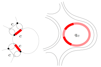
Figure 4: One-loop divergent graph, $n_{4}^{(c)}$ at $d=3$ contributing to the flow of $\lambda$.

Explicitly, at one-loop,

$$K_{n_{4}^{(c)}}=2\,,$$ (89)

$$S_{n_{4}^{(c)}}(\{\mathbf{p},\mathbf{p}^{\prime}\})=\frac{1}{2!}\Big{(}\frac{-\lambda^{(c)}_{+}}{2}\Big{)}^{2}\sum_{q_{c}}\frac{|q_{c}|^{2a}}{(|\mathbf{p}_{\check{c}}|^{2b}+|q_{c}|^{2b}+\mu)}\frac{|q_{c}|^{2a}}{(|\mathbf{p}^{\prime}_{\check{c}}|^{2b}+|q_{c}|^{2b}+\mu)}\,,$$ (90)

where $\mathbf{p}_{\check{c}}=(p_{1},\dots,p_{c-1},p_{c+1},\dots,p_{d})$, and $|\mathbf{p}_{\check{c}}|^{2b}=\sum_{l=1|l\neq c}^{d}p_{l}^{2b}$.

We compile these equations and deliver the $\beta$-functions of the couplings up to one-loop as

$$\lambda^{(c)}_{\rm ren}=\lambda^{(c)}-\frac{1}{4}(\lambda^{(c)}_{+})^{2}S_{0}\,,\qquad\quad S_{0}=\sum_{q}\frac{|q|^{4a}}{(|q|^{2b}+\mu_{i})^{2}}\,,$$ (91)

$$\lambda^{(c)}_{\rm+;ren}=\lambda^{(c)}_{+}\,,$$ (92)

where $\lambda_{\rm ren}$ and $\lambda_{+,{\rm ren}}$ are the obvious corresponding renormalized coupling constant. We set all couplings to $\lambda^{(c)}=\lambda$, and $\lambda^{(c)}_{+}=\lambda_{+}$ to simplify these

$$\lambda_{\rm ren}=\lambda-\frac{1}{4}(\lambda_{+})^{2}S_{0}\,,$$ (93)

$$\lambda_{+;{\rm ren}}=\lambda_{+}\;.$$ (94)

These RG flow equations carry already some information. The second equation displays the fact that the marginal coupling $\lambda_{+}$ does not run and defines a fixed point at all orders of perturbation. These equations also reflect that the two couplings $\lambda$ and $\lambda_{+}$ could not be set the same (assuming equal value of the couplings is inconsistent with these equations).

We want to understand the qualitative feature of RG flow given by the above coupled system. In the multiscale analysis with discrete scale $i$, the system can be written as

$$\lambda_{i-1}=\lambda_{i}-\frac{1}{4}\lambda_{+,i}^{2}S_{0,i}\,,$$ (95)

$$\lambda_{+,i-1}=\lambda_{+,i}\,,$$ (96)

where $S_{0,i}$ stands for the cut-off amplitude of the formal sum $S_{0}$ and formulates as

$$S_{0,i} = \sum_{q}|q|^{4a}\int_{0}^{\infty}d\alpha\chi^{i}(\alpha)e^{-\alpha(|q|^{2b}+\mu_{i})}\int_{0}^{\infty}d\alpha^{\prime}\chi^{i}(\alpha^{\prime})e^{-\alpha^{\prime}(|q|^{2b}+\mu_{i})}$$ (97)

$$= \int_{0}^{\infty}d\alpha\,\chi^{i}(\alpha)\int_{0}^{\infty}d\alpha^{\prime}\chi^{i}(\alpha^{\prime})e^{-(\alpha+\alpha^{\prime})\mu_{i}}\sum_{q}|q|^{4a}e^{-(\alpha+\alpha^{\prime})|q|^{2b}}\,,$$ (98)

where the sharp cutoff function $\chi^{i}(\alpha)$ was defined in (63).

On scaling dimensions. Computing $\beta$-functions of our different couplings at first order of perturbation and solving them, we must deliver these equations using dimensionless couplings.

Using Peskin and Schroeder’s argument [43], the scaling dimensions of a coupling $g_{\bullet}$ can be read from the degree of divergence as ($-1$ times) the coefficient of the corresponding vertex number $V_{\bullet}$. The same argument has been extended to the scaling of TFT couplings according to [34]. This agrees also with the scaling dimension of field and coupling using integrability arguments, see for instance [44], for applications involving both stochastic analysis in the TFT setting.

Denoting the scaling dimension of a coupling $g$ by $\{g\}$, and using (40), we have

$$\{\lambda_{+}\}=-(d-1-4b+2a)=0\;,\qquad\{\lambda\}=-(d-1-4b)=2a=d-2\;,$$ (99)

$$\{\mu\}=2b=d-\frac{3}{2}\;,\qquad\{Z_{a}\}=2(b-a)=\frac{1}{2}\;,$$ (100)

where the vanishing of the first scaling dimension is due to the marginality of $\lambda_{+}$. The dimensions also show that both $\lambda$ and $Z_{a}$ define relevant directions.

Perturbative $\beta$-function and integration. First, we give an approximation of $S_{0,i}$ (98). The sum over $q$ will be handled using an integral via Euler-Maclaurin approximation (Appendix A details the following result):

$$S_{0,i}=\frac{1}{b}\log\frac{(M^{2b}+1)^{2}}{4M^{2b}}+{\mathcal{O}}(M^{-2bi}\log(M^{-2bi}))\,.$$ (101)

We write the $\beta$-function for a given coupling $g$ as $\beta_{g}(k)=k\partial_{k}g(k)$, where $k$ is a momentum scale. In our present setting dealing with discrete slices (multiscale analysis), we have finite difference equations that we will turn into differential equation. The momentum scale must be compared to the slice range as $k/k_{0}\sim M^{i}$, given in terms of a given momentum unit $k_{0}$. Using the so-called time scale $t=\log(k/k_{0})\sim i\log M$, given that the coupling $\lambda_{+}=\lambda_{+,i}$ does not run and that, at leading order $S_{0,i}=c\log M$, where $c>0$, the difference $\lambda_{i-1}-\lambda_{i}$ takes the form:

$$-(\lambda_{i-1}-\lambda_{i})=\frac{\partial\lambda_{i}}{\partial i} = \frac{1}{4}\lambda_{+,i}^{2}\,S_{0,i}\,,$$ (102)

which can be translated into the following first order ODE

$$\frac{\partial\lambda_{i}}{\partial((\log M)i)}=\partial_{t}\lambda(t) = -\beta_{\lambda}\lambda_{+}^{2}$$ (103)

$$\beta_{\lambda} = -\frac{1}{4b}\frac{\log\frac{(M^{2b}+1)^{2}}{4M^{2b}}}{\log(M)}<0\,.$$ (104)

One may wonder why $M$, the propagator slice parameter, appears in the perturbative expansion and if the present equation does not depend on the slicing scheme. The multi-scale analysis justifies this entirely: we are computing a flow between two scales $\sim M^{-2bi}$, therefore $M$ becomes an input of our equation.

Using the scaling dimensions (100), we have $S_{0,i}=\widetilde{S}_{0,i}$, $\lambda=k^{d-2}\widetilde{\lambda}$ and $\lambda_{+}=\widetilde{\lambda}_{+}$, where $\;\widetilde{}\;$ indicates a dimensionless quantity. Then, we obtain $\partial_{t}\lambda=(d-2)k^{d-2}\widetilde{\lambda}+k^{d-2}\partial_{t}\widetilde{\lambda}$ and

$$\partial_{t}\widetilde{\lambda}=-(d-2)\widetilde{\lambda}+k^{-(d-2)}|\beta_{\lambda}|\lambda_{+}^{2}\,.$$ (105)

We use $k=k_{0}e^{t}$, and any equation dependence in the unit of momentum $k_{0}$ will be confined to a single constant $c_{0}$ (though, this constant may vary from equation to equation). Massaging (105),

$$\partial_{t}(e^{(d-2)t}\widetilde{\lambda})=c_{0}|\beta_{\lambda}|\lambda_{+}^{2}\,.$$ (106)

Now, we integrate the equation to obtain

$$\widetilde{\lambda}(t) = c_{0}|\beta_{\lambda}|\lambda_{+}^{2}\,t\,e^{-(d-2)t}+const.\,e^{-(d-2)t}$$ (107)

$$= c_{0}|\beta_{\lambda}|\lambda_{+}^{2}(t-t_{0})\,e^{-(d-2)t}+\widetilde{\lambda}(t_{0})\,e^{-(d-2)(t-t_{0})}$$ (108)

where the initial condition was set at some IR scale $e^{t_{0}}\ll\Lambda/k_{0}=e^{t}$.

As opposed to the usual $\phi^{4}_{4}$ model, there is no pole in the solution at first order. This proves that there is no Landau ghost and therefore this model is not similar to the ordinary $\phi^{4}_{4}$ model. Furthermore, at large $t\geq t_{0}$, $\widetilde{\lambda}(t)$ becomes suppressed by the exponential factors. This is of course the ordinary behavior of relevant couplings. One may be tempted to conclude to asymptotic freedom, however, we will show that another coupling does not run to 0. In the IR, $t\to-\infty$, $\lambda$ grows and such that we may expect phase transition in this regime. Note also that the resulting model differs from the usual $T^{4}$-TFT model with only $\lambda$ coupling. Indeed, the latter describes a different class of dominant graphs (melonic ones) yielding asymptotic freedom via a marginal coupling. Finally, at $d=2$, something special happens. Of course, this is an (enhanced) matrix model which enhances some planar graphs. This deserves a full-fledged investigation.

3.3 Computing $\Gamma_{2}$ and $Z_{a}$ RG equation

Now we compute the renormalization of the $2$-point coupling, $\Gamma_{2}^{(c)}(\{0\})$, at fixed color $c$:

$$|p_{c}|^{2a}\Gamma_{2}^{(c)}(\{p\}) = \sum_{{\cal G}_{2;a;\iota}^{(c)}}K_{{\cal G}_{2;a;\iota}^{(c)}}S_{{\cal G}_{2;a;\iota}^{(c)}}(\{p\})\,,$$ (109)

where the sum is over all amputated $1$PI $2$-point graphs at $1$-loop whose boundaries to be in the form of ${\rm Tr}_{2;(c)}({p}^{2a}\phi^{2})$.

Up to the first order in perturbation theory, we have ${\cal G}_{2;a;\iota}^{(c)}\in\{z_{a}^{(c)},m_{e}^{(c)}\}$, where $z_{a}^{(c)}$ is the leading order (zero-loop) graph with one $Z_{a}^{(c)}$ interaction with two external legs. (Appendix B shows additional graphs up to the second order in perturbation theory.) In (72), we have identified $\partial_{|p_{c}|^{2a}}\Sigma|_{\{p\}=0}\equiv\Gamma^{(c)}_{2}(\{0\})$ as divergent. The other contributing graphs, namely $m_{e}^{(c)}$, $c=1,2,3$, are divergent at first order in perturbation theory (row II of Table 1) with $\omega_{m_{e}^{(c)}}=\frac{D}{2}$.

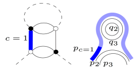
Figure 5: Illustration of $m_{e}^{(c=1)}$ for $d=3$ in colored (left) and stranded (right) representations. $\{q_{\check{c}}\}=\{q_{2},\;q_{3}\}$, ${|{\bf q}_{\check{c}}|}^{2b}={|q_{2}|}^{2b}+{|q_{3}|}^{2b}$.

$$K_{m_{e}^{(c)}}S_{m_{e}^{(c)}}(\{p\}) = K_{m_{e}^{(c)}}\Big{(}-\frac{{\lambda_{+}}^{(c)}}{2}\Big{)}\sum_{\{q_{\check{c}}\}}\frac{|p_{c}|^{2a}}{({|{\bf q}_{\check{c}}|}^{2b}+|p_{c}|^{2b}+\mu)}\,,$$ (110)

where $K_{m_{e}^{(c)}}=2$. Putting all together, up to first order in perturbation theory,

$$|p_{c}|^{2a}\Gamma_{2}^{(c)}(\{p\})=-|p_{c}|^{2a}Z_{a}^{(c)}-\lambda_{+}^{(c)}|p_{c}|^{2a}\sum_{\{q_{\check{c}}\}}\frac{1}{({|{\bf q}_{\check{c}}|}^{2b}+{|p_{c}|}^{2b}+\mu)}\,.$$ (111)

$\Gamma_{2}^{(c)}(\{p\})$ is therefore identified easily. For general $d$, recalling the renormalization group equations (87) and setting all the external momenta $\{p\}=0$, we obtain:

$$Z^{(c)}_{a,{\rm ren}} = -\Gamma^{(c)}_{2}(\{0\})=Z^{(c)}_{a}+\lambda_{+}^{(c)}\sum_{\{q_{\check{c}}\}}\frac{1}{({|{\bf q}_{\check{c}}|}^{2b}+\mu)}\,.$$ (112)

Note that we only keep the first order in Taylor expansion in couplings. Setting the couplings independent of colors,

$$Z_{a,{\rm ren}} = Z_{a}+\lambda_{+}\sum_{\{q_{1},\dots,q_{d-1}\}}\frac{1}{({|{\bf q}|}^{2b}+\mu)}\,.$$ (113)

In the multiscale analysis language,

$$Z_{a,i-1}=Z_{a,i}+\lambda_{+,i}S_{1,i}\,,$$ (114)

where $S_{1,i}$ is given in (132) with explicit expression given in (134), where we fixed $D=1$. We recall that $\lambda_{+}=\lambda_{+,i}$ does not run. Making explicit the dimensions, we obtain the renormalization group equation for $Z_{a}$ as

$$Z_{a,i-1}=Z_{a,i}+k^{1/2}\lambda_{+,i}\,\widetilde{S}_{1,i}\,,$$ (115)

which, using $\widetilde{S}_{1,i}$ given in (A.50), gives the $\beta$-function for $Z_{a}$:

$$-(Z_{a,i-1}-Z_{a,i}) = \frac{\partial Z_{a,i}}{\partial i}=-k^{1/2}\lambda_{+,i}\,\widetilde{S}_{1,i}\,,$$ (116)

$$\frac{\partial Z_{a,i}}{\partial((\log M)i)} = \partial_{t}Z_{a}(t)=-k^{1/2}\beta_{Z_{a}}\,\lambda_{+}\,,$$ (117)

$$\beta_{Z_{a}} = \frac{\widetilde{S}_{1,i}}{\log(M)}>0\,.$$ (118)

Introducing dimensionless quantities, $Z_{a}(t)=k^{1/2}\widetilde{Z}_{a}(t)$, the dimensionless RG equation can be written

$$\partial_{t}\widetilde{Z}_{a}(t) = -\frac{1}{2}\widetilde{Z}_{a}(t)+k^{-1/2}\partial_{t}Z_{a}(t)$$ (119)

$$= -\frac{1}{2}\widetilde{Z}_{a}(t)-\beta_{Z_{a}}\,\lambda_{+}\,.$$ (120)

This integrates easily with respect to $t$ and gives

$$\widetilde{Z}_{a}(t)=c_{1}\,e^{-t/2}-2\beta_{Z_{a}}\,\lambda_{+}\,,$$ (121)

where $c_{1}$ is an integration constant. This equation just expresses the fact that $\widetilde{Z}_{a}(t)$ is a relevant coupling and decreases exponentially in the UV ($t\rightarrow\infty$) and suppressed up to reach a constant $-2\beta_{Z_{a}}\,\lambda_{+}$. This and the fact that $\lambda_{+}$ is a constant make this model not asymptotically free although the coupling $\widetilde{\lambda}$ flows to 0. On the other hand, in the IR ($t\rightarrow-\infty$), $\widetilde{Z}_{a}(t)$ blows up as any relevant coupling.

3.4 Self energy and mass RG equation

Our following task is to compute the so-called self energy, which we denote by $\Sigma_{b}(\{p\})$:

$$\Sigma_{b}(\{p\})=\sum_{c=1}^{d}\sum_{{\cal G}^{(c)}_{2,\iota}}{K_{{\cal G}^{(c)}_{2,\iota}}}{S_{{\cal G}^{(c)}_{2,\iota}}}(\{p\})\,,$$ (122)

where the first sum is broken by color $c$ and the second sum is performed over all amputated 1PI 2-point graphs ${\cal G}^{(c)}_{2,\iota}$ (with color label $c$) at 1-loop with boundary to be in the form of ${\rm Tr}_{2}(p^{2b}\phi^{2})$ (hence the index $b$ in subscript in $\Sigma_{b}(\{p\})$).

It is noteworthy that $\Sigma_{b}(\{p\})$ corresponds to the part $\Sigma(\{0\})+\sum_{c}|p_{c}|^{2b}\partial_{|p_{c}|^{2b}}\Sigma\big{|}_{\{p\}=0}$ of total self-energy function $\Sigma(\{p\})$ in (72). Noting that the second term $\partial_{|p_{c}|^{2b}}\Sigma\big{|}_{\{p\}=0}=0$, we only focus on the contribution $\Sigma(\{0\})$, namely the contribution to the mass renormalization.

The graphs we are interested in are denoted ${{\cal G}^{(c)}_{2,\iota}}\in\{m^{(c)},n^{(c)}\}_{c=1,2,\dots,d}$, see Figures 6 and 7.

• For the graph $m^{(c)}$, $c=1,\dots,d$, the degree of divergence $\omega_{d;+}(m^{(c)})$ reaches $\frac{D}{2}$, as shown in the class III of Table 1. In Figure 6, we display $m^{(c)}$, when the vertical line is color $c$.

  

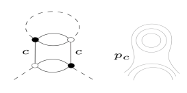
  Figure 6: The graph $m^{(c)}$ in the case $d=3$ in colored (left) and stranded (right) representations.

  The contribution to the amplitude brought by the graphs $m^{(c)}$ is

  $$\sum_{c=1}^{d}K_{m^{(c)}}S_{m^{(c)}}(\{p\}) = \sum_{c=1}^{d}2\big{(}-\frac{\lambda^{(c)}}{2}\big{)}\sum_{\{q_{\check{c}}\}}\frac{1}{({|{\bf q}_{\check{c}}|}^{2b}+|p_{c}|^{2b}+\mu)}$$ (123)

  $$= \sum_{c=1}^{d}\sum_{\{q_{\check{c}}\}}(-\lambda^{(c)})\frac{1}{({|{\bf q}_{\check{c}}|}^{2b}+|p_{c}|^{2b}+\mu)}\,,$$ (124)

  where $K_{m^{(c)}}=2$, for any $c$.

• In the second class of graphs denoted each $n^{(c)}$, the amplitude has divergence degree $\omega_{d;+}(n^{(c)})=\frac{D}{2}$. This graph belongs to the class I in Table 1. Figure 7 shows $n^{(c)}$ at order $d=3$ with horizontal line colored by index $c$.

  

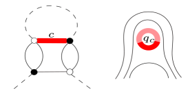
  Figure 7: $n^{(c)}$ for $d=3$ in colored (left) and stranded (right) representations.

  The sum of Feynman amplitude associated with the graph $n{(c)}$ yields

  $$\sum_{c=1}^{d}K_{n^{(c)}}S_{n^{(c)}}(\{p\}) = \frac{1}{2}\sum_{c=1}^{d}(-\lambda_{+}^{(c)})\sum_{q_{c}}\frac{|q_{c}|^{2a}}{(|q_{c}|^{2b}+{|{\bf p}_{\check{c}}|}^{2b}+\mu)}\,,$$ (125)

  where $K_{n^{(c)}}=1$ for any $c$.

Up to the first order in perturbation theory and evaluating at $0$ external momenta, we obtain

$$\Sigma_{b}(\{0\})=\sum_{c=1}^{d}\Big{(}K_{m^{(c)}}S_{m^{(c)}}(\{p\})+K_{n^{(c)}}S_{n^{(c)}}(\{p\})\Big{)}\Big{|}_{p=0}$$ (126)

$$=\sum_{c=1}^{d}\Big{[}(-\lambda^{(c)})\sum_{\{q_{\check{c}}\}}\frac{1}{({|{\bf q}_{\check{c}}|}^{2b}+\mu)}+\frac{1}{2}(-{\lambda_{+}}^{(c)})\sum_{q_{c}}\frac{|q_{c}|^{2a}}{(|q_{c}|^{2b}+\mu)}\Big{]}$$ (127)

Therefore, for general $d$, the renormalized mass equation up to the first order in perturbation is given by:

$${\mu_{\rm ren}}=\mu+\sum_{c=1}^{d}\Bigg{\{}\lambda^{(c)}\sum_{\{q_{\check{c}}\}}\frac{1}{({|{\bf q}_{\check{c}}|}^{2b}+\mu)}+\frac{1}{2}{\lambda_{+}}^{(c)}\sum_{q_{c}}\frac{|q_{c}|^{2a}}{(|q_{c}|^{2b}+\mu)}\Bigg{\}}\,.$$ (129)

Now assert color independence, namely $\lambda^{(c)}=\lambda$, ${\lambda_{+}}^{(c)}=\lambda_{+}$, one gets

$$\mu_{\rm ren}=\mu+d\Big{(}\lambda S_{1}\>+\;\frac{1}{2}{\lambda_{+}}S_{2}\Big{)}$$ (130)

$$S_{1}=\sum_{\{q_{1},\dots,q_{d-1}\}}\frac{1}{({|{\bf q}|}^{2b}+\mu)}\qquad S_{2}=\sum_{q}\frac{|q|^{2a}}{(|q|^{2b}+\mu)}\,,$$ (131)

where we restrict ourselves to $D=1$.

We cut off the propagators, switch to dimensionful quantities, and write the sums

$$S_{1,i}=\sum_{{\bf q}\in k{\mathbbm{Z}}^{d-1}}\int_{0}^{\infty}d\alpha\;\chi^{i}(\alpha)\,e^{-\alpha(|{\bf q}|^{2b}+\mu_{i})}\,,$$ (132)

$$S_{2,i}=\sum_{q\in k{\mathbbm{Z}}}\int_{0}^{\infty}d\alpha\;\chi^{i}(\alpha)\,|q|^{2a}e^{-\alpha(|q|^{2b}+\mu_{i})}\,.$$ (133)

In writing explicitly the dimensions of $q$ and $\alpha$ in terms of momentum scale $k$, (A.58) in Appendix A proves that we can approximate those as

$$S_{1,i}=k^{1/2}\Bigg{(}\Big{(}\frac{1}{b}\Gamma\left(\frac{1}{2b}\right)\Big{)}^{d-1}(2d-3)\Big{(}1-M^{-1/2}\Big{)}M^{i/2}+{\mathcal{O}}(M^{-i/2})\Bigg{)}\,,$$ (134)

$$S_{2,i}=k^{1/2}\Bigg{(}4\,\Gamma\Big{(}\frac{2(d-1)}{2d-3}\Big{)}(1-M^{-1/2})M^{i/2}+{\mathcal{O}}\big{(}M^{-i(d-2)}\big{)}\Bigg{)}\,,$$ (135)

where we have set $D=1$ at any order $d$ and $b=\frac{1}{2}(d-\frac{3}{2})$ given in Proposition 1. Compiling this, we obtain the following equation at leading order,

$$\mu_{i-1} = \mu_{i}+k^{1/2}d\Big{(}\lambda_{i}\widetilde{S}_{1,i}+\frac{1}{2}\lambda_{+,i}\widetilde{S}_{2,i}\Big{)}\,,$$ (136)

$$\widetilde{S}_{1,i} = k^{-1/2}S_{1,i}\,,$$ (137)

$$\widetilde{S}_{2,i} = k^{-1/2}S_{2,i}\,.$$ (138)

We obtain the $\beta$-function for the mass

$$-(\mu_{i-1}-\mu_{i}) = \frac{\partial\mu_{i}}{\partial i}=-k^{1/2}d\Big{(}\widetilde{S}_{1,i}\,\lambda_{i}+\frac{1}{2}\widetilde{S}_{2,i}\,\lambda_{+,i}\Big{)}\,,$$ (139)

$$\frac{\partial\mu_{i}}{\partial((\log M)i)} = \partial_{t}\mu=-k^{1/2}(\beta_{\mu,1}\,\lambda+\beta_{\mu,2}\,\lambda_{+})\,,$$ (140)

$$\beta_{\mu,1} = \frac{d}{\log M}\,\widetilde{S}_{1,i}>0\,,$$ (141)

$$\beta_{\mu,2} = \frac{d}{2\,\log M}\,\widetilde{S}_{2,i}>0\,.$$ (142)

According to (100), we recall the scaling dimensions $\{\mu\}=2b=d-3/2$, $\{\lambda_{+}\}=0$ and $\{\lambda\}=2a=d-2$. We therefore switch to dimensionless quantities, $\mu=k^{d-\frac{3}{2}}\widetilde{\mu}$, therefore, $\partial_{t}\mu=k^{d-\frac{3}{2}}((d-\frac{3}{2})\widetilde{\mu}+\partial_{t}\widetilde{\mu})$. This equation becomes

$$\partial_{t}\widetilde{\mu}(t)=-(d-\frac{3}{2})\widetilde{\mu}(t)+k^{-(d-\frac{3}{2})}\partial_{t}\mu(t)\,.$$ (143)

Given that the coupling $\lambda_{+}=\lambda_{+,i}$ does not run and that, $\widetilde{\lambda}$ runs according to (108), we make the $t$ dependence explicit and

$$\partial_{t}\widetilde{\mu}(t) = -(d-\frac{3}{2})\widetilde{\mu}(t)-(\beta_{\mu,1}\,\tilde{\lambda}(t)+c_{0}e^{-(d-2)t}\,\beta_{\mu,2}\,\lambda_{+})$$ (144)

$$= -(d-\frac{3}{2})\widetilde{\mu}(t)\,-\left(\beta_{1}(t-t_{0})+\beta_{2}\right)e^{-(d-2)t}\,,$$ (146)

where $\beta_{1}=c_{0}\beta_{\mu,1}\,|\beta_{\lambda}|\,\lambda_{+}^{2}$, $\beta_{2}=\beta_{\mu,1}\tilde{\lambda}(t_{0})e^{(d-2)t_{0}}+c_{0}\beta_{\mu,2}\,\lambda_{+}$. The above differential equation (144) takes the form:

$$\partial_{t}(e^{(d-\frac{3}{2})t}\widetilde{\mu}(t))=-e^{\frac{1}{2}t}\left(\beta_{1}(t-t_{0})+\beta_{2}\right)\,.$$ (147)

We integrate this and obtain

$$\widetilde{\mu}(t) = -2e^{-(d-2)t}\Big{(}\beta_{1}(t-t_{0})+(-2\beta_{1}+\beta_{2})\Big{)}+const.e^{-(d-\frac{3}{2})t}\,,$$ (148)

with

$$const.=e^{(d-\frac{3}{2})t_{0}}\widetilde{\mu}(t_{0})+2e^{\frac{1}{2}t_{0}}\Big{(}-2\beta_{1}+\beta_{2}\Big{)}\,.$$ (149)

In the UV, $\widetilde{\mu}$ runs to $0$ whereas in the IR the mass exponentially increases. This behavior is common to any relevant mass coupling.

Summary – We list our dimensionless 1-loop RG flow equations for the model $+$ and their solutions below. The constants $\kappa_{i}$, $i=1,2,3,4$, are integration constants.

$\partial_{t}\,\widetilde{\lambda}(t)=-(d-2)\widetilde{\lambda}(t)+c_{0}|\beta_{\lambda}|\lambda_{+}^{2}e^{-(d-2)t}$	$\widetilde{\lambda}(t)=e^{-(d-2)t}(c_{0}|\beta_{\lambda}|\,\lambda_{+}^{2}\,t+\kappa_{1})$
$\partial_{t}\,\lambda_{+}=0$	$\lambda_{+}=\kappa_{2}$
$\partial_{t}\,\widetilde{\mu}(t)=-(d-\frac{3}{2})\widetilde{\mu}(t)$	$\widetilde{\mu}(t)=2e^{-(d-2)t}\big{[}-\beta_{1}\,t+\gamma\big{]}+\kappa_{3}e^{-(d-\frac{3}{2})t}$
$-(\beta_{\mu,1}\,\widetilde{\lambda}(t)+c_{0}e^{-(d-2)t}\beta_{\mu,2}\,\lambda_{+})$	$\beta_{1}=c_{0}\beta_{\mu,1}|\beta_{\lambda}|\lambda_{+}^{2}>0$ ,
$\beta_{\mu,1}>0\,,\;\,c_{0}\beta_{\mu,2}>0$	$\gamma=\beta_{1}(t_{0}+2)-\beta_{2}$
	$\beta_{2}=\beta_{\mu,1}\tilde{\lambda}(t_{0})e^{(d-2)t_{0}}+c_{0}\beta_{\mu,2}\,\lambda_{+}$
$\partial_{t}\,\widetilde{Z}_{a}(t)=-\frac{1}{2}\widetilde{Z}_{a}(t)-\beta_{Z_{a}}\,\lambda_{+}$ ,  $\beta_{Z_{a}}>0$	$\widetilde{Z}_{a}(t)=\kappa_{4}\,e^{-t/2}-2\beta_{Z_{a}}\,\lambda_{+}$

Table 3: Summary of the RG flow equations for the couplings in the model $+$.

3.5 Integration at arbitrary loops

The power counting of the model $+$, provided by Proposition 1, gives us a lot of information about the $\beta$-functions of the couplings even in at arbitrarily high order of perturbation theory. In this section, we investigate general forms of the $\beta$-functions of the couplings in the model $+$ at all orders of perturbation theory.

4-point couplings $\lambda$ and $\lambda_{+}$ RG equation – Proposition 1 dictates that there are no diverging amplitudes contributing to the renormalization of $\lambda_{+}$ at all orders in perturbation, therefore, $\lambda_{+}$ is constant at all orders. Furthermore, from the first row of Table 1 of Proposition 1, which governs the renormalization of the coupling $\lambda$, we know that in order for the amplitude to be divergent, Feynman graph must only contain $\lambda_{+}$ couplings, and no other couplings. Then, we can readily conclude that, the subleading corrections to $\lambda$ at $n$-loops, $n$ being arbitrary, can be written as a polynomial $P_{n}(\lambda_{+})$ in the variable $\lambda_{+}$ that is fixed to a constant. At arbitrary $n$-th order in perturbation, the $\beta$-function of the coupling $\lambda$ assumes the form

$$\partial_{t}\lambda(t)=P_{n}(\lambda_{+})$$ (150)

and that can be integrated in terms of dimensionless coupling as

$$\widetilde{\lambda}(t)=e^{-(d-2)t}(P_{n}(\lambda_{+})t+const.)\,.$$ (151)

The particular form of $P_{n}(\lambda_{+})=-\beta_{\lambda}\lambda_{+}^{2}+\dots$ is left for future investigation. However whatever form $P_{n}(\lambda_{+})$ may have, the asymptotic behavior of $\widetilde{\lambda}$ remains unchanged: it vanishes in the UV.

2-point coupling $Z_{a}$ RG equation – The classes II and V of Proposition 1 contribute to the renormalization of the $2$-point coupling $Z_{a}$. All class II amplitudes involve only the coupling $\lambda_{+}$ yielding a similar result as to the one-loop computation above. The class V contains contributions with exactly one $Z_{a}$ and several $\lambda_{+}$ (an example is given in Fig. 12 Appendix B). Therefore, at an arbitrary $n$-th order in perturbation theory, we expect

$$\partial_{t}Z_{a}(t) = e^{t/2}Q_{1;n}(\lambda_{+})+t\,Q_{2;n}(\lambda_{+})\,Z_{a}(t)\,,$$ (152)

where $Q_{i;n}(\lambda_{+})$, $i=1,2$ are polynomials in $\lambda_{+}$. This equation can be integrated but we refrain to display the solution.

Mass RG equation – Looking at Proposition 1, the classes that contribute to the renormalization of the mass are I, III, IV, and VI. The class I only contains $\lambda_{+}$, which is held constant. The class III contains only exactly one $\lambda$ and the rests are all $\lambda_{+}$. The class IV contains only exactly one $Z_{a}$ coupling and the rests are all $\lambda_{+}$. Finally, the class VI contains exactly only one $Z_{a}$, and exactly only one $\lambda$, and the rests are $\lambda_{+}$. Noting that $\lambda_{+}$ does not run at all orders, the most complicated one could have is the class VI where $\lambda$ and $Z_{a}$ are coupled (whose example is given in Fig.14). Therefore, we expect

$$\partial_{t}\mu(t) = e^{t/2}\Big{(}R_{1;n}(\lambda_{+})\,\lambda(t)+R_{2;n}(\lambda_{+})\Big{)}+\,t\,Z_{a}(t)\Big{(}R_{3;n}(\lambda_{+})\lambda(t)\,+R_{4;n}(\lambda_{+})\Big{)}\,,\qquad$$ (153)

to an arbitrary $n$-th order in perturbation theory, and $R_{i;n}$, with $i=1,2,3,4$ are polynomials in $\lambda_{+}$.

In summary, we expect that the coupled system of RG equations of the model $+$ to an arbitrary $n$-th order is given in terms of dimensionful couplings as

$$\partial_{t}\lambda_{+} = 0\,,$$ (154)

$$\partial_{t}\lambda(t) = P_{n}(\lambda_{+})\,,$$ (155)

$$\partial_{t}Z_{a}(t) = e^{t/2}Q_{1;n}(\lambda_{+})+t\,Z_{a}(t)Q_{2;n}(\lambda_{+})\,,$$ (156)

$$\partial_{t}\mu(t) = e^{t/2}\Big{(}R_{1;n}(\lambda_{+})\,\lambda(t)+R_{2;n}(\lambda_{+})\Big{)}+\,t\,Z_{a}(t)\Big{(}R_{3;n}(\lambda_{+})\lambda(t)\,+R_{4;n}(\lambda_{+})\,\Big{)}\,.\qquad$$ (157)

Apart from $\widetilde{\lambda}$, the solution of these equations requires more asumptions before interpreting the UV asymptotic behavior of the model. For instance, the behavior of $\widetilde{Z}_{a}$ strongly depends on $Q_{2;n}$ that is yet unknown.

4 One-loop beta-functions of the model $\times$

Just as performed for the model $+$, we will compute the 1-loop RG flow equations of coupling constants via multiscale analysis for the model $\times$. Because the scheme and proofs are nearly identical, the derivations and explanations are given in a streamlined analysis. We stress the following fact: although the notation and expressions are similar to previous section, they actually refer to different quantities. As the model is different, there is no confusion and no need to introduce new notation.

4.1 Effective coupling equations

The integration of high modes yields a formal effective action of the form (71) where notation keeps its meaning but adapts to the present model. Therein, the 2-point amplitudes expand in local and nonlocal parts, obtaining, a self-energy of the same form as given in (72) in addition with the following term:

$$\sum_{c}|p_{c}|^{4a}\partial_{|p_{c}|^{4a}}\Sigma\big{|}_{\{p\}=0}\,.$$ (158)

According to [35], Table 2 dictates the renormalization analysis of the model. One shows that

$$\partial_{|p_{c}|^{2b}}\Sigma\big{|}_{\{p\}=0}=0 \qquad\text{implies }\;Z_{b}=1\quad\text{wave function renormalization}$$ (159)

$$\Sigma(\{0\})\sim\log-{\rm divergent}$$ (row III)  mass renormalization (160)

$$\partial_{|p_{c}|^{2a}}\Sigma|_{\{p\}=0}\equiv\Gamma^{(c)}_{2;a}(\{0\})\sim\log-{\rm divergent} \qquad\text{(row I) \quad}Z_{a}\text{\; renormalization}$$ (161)

$$\partial_{|p_{c}|^{4a}}\Sigma|_{\{p\}=0}\equiv\Gamma^{(c)}_{2;2a}(\{0\})\sim\log-{\rm divergent} \qquad\text{(row II) \quad}Z_{2a}\text{\; renormalization}$$ (162)

where $|p_{c}|^{2a}\Gamma^{(c)}_{2;a}(\{p\})$ and $|p_{c}|^{4a}\Gamma^{(c)}_{2;2a}(\{p\})$ are the sum of all amputated 1PI 2-point functions following the patterns of ${\rm Tr}_{2;c}({p}^{2a}\phi^{2})$ and ${\rm Tr}_{2;c}({p}^{4a}\phi^{2})$, respectively, on their boundary graphs. Because $4$-point functions converge we do not need to report them.

We reorganize the effective action as

$$-W^{i-1}(\phi_{\leq i-1},{\bar{\phi}}_{\leq i-1}) = \Sigma_{i-1}(\{0\}){\rm Tr}_{2}(\phi^{2}_{\leq i-1})+\sum_{c}\Gamma^{(c)}_{2;a,\;i-1}(\{0\}){\rm Tr}_{2;c}({p}^{2a}\phi^{2}_{\leq i-1})$$ (164)

$$+\sum_{c}\Gamma^{(c)}_{2;2a,\;i-1}(\{0\}){\rm Tr}_{2;c}({p}^{4a}\phi^{2}_{\leq i-1})+{\tilde{R}}(\phi_{\leq i-1})\,,$$

where ${\tilde{R}}(\phi_{\leq i-1})$ contains all finite contributions.

Following step by step, the previous analysis, we deliver the the effective couplings at scale $i-1$:

$$Z_{b,\,i-1} = 1\,,$$ (165)

$$\mu_{{\rm ren},i-1} = \mu_{i-1}-\Sigma_{i-1}(\{0\})\,,$$ (166)

$$Z_{a,i-1} = -\Gamma^{(c)}_{2;a,i-1}(\{0\})\,,$$ (167)

$$Z_{2a,i-1} = -\Gamma^{(c)}_{2;2a,i-1}(\{0\})\,,$$ (168)

Following Proposition 2, we work with the set of parameters $d=3$, $D=1$, $a=\frac{1}{2}$, and $b=1$ so that the model is just-renormalizable.

4.2 Self energy and mass RG equation

For the model $\times$, we calculate the self energy which we denote again by $\Sigma_{b}(\{p\})$ and which has an expression similar to (122), where the graphs ${\cal G}^{(c)}_{2,\iota}$ should be chosen among all amputated 1PI 2-point graphs with boundary of the form ${\rm Tr}_{2;c}(p^{2b}\phi^{2})$.

Up to the first order in perturbation theory, ${\cal G}^{(c)}_{2,\iota}\in\{m^{(1)},m^{(2)},m^{(3)}\}$. (At second order in perturbation theory, the interested reader may look at Fig. 18 in Appendix C.)

Recall that $\Sigma_{b}(\{p\})$ corresponds to $\Sigma(\{0\})+\sum_{c}|p_{c}|^{2b}\partial_{|p_{c}|^{2b}}\Sigma\big{|}_{\{p\}=0}$. Considering that the second term vanishes, i.e. $\partial_{|p_{c}|^{2b}}\Sigma\big{|}_{\{p\}=0}=0$, only the contribution $\Sigma(\{0\})$, namely the mass renormalization, survives.

For $m^{(c)}$, $c=1,2,3$, $\omega_{d;\times}({m^{(c)}})=0$. This graph belongs to the class III in Table 2, also, it appears at first order.

Figure 8: The graph $m^{(c)}$. In the case $d=3$. ${|{\bf q}_{\check{c}}|}^{2b}=|q_{1}|^{2b}+|q_{2}|^{2b}$. Here the parameters should follow that of Proposition 2.

We sum the contributions of the graphs $m^{(c)}$ and write:

$$\Sigma_{b}(\{p\})=\sum_{c=1}^{d}K_{m^{(c)}}S_{m^{(c)}}(\{p\}) = \sum_{c=1}^{d}2\big{(}-\frac{\lambda^{(c)}}{2}\big{)}\sum_{\{q_{\check{c}}\}}\frac{1}{({|{\bf q}_{\check{c}}|}^{2b}+p^{2b}_{c}+\mu)}\,,$$ (169)

where $K_{m^{(c)}}=2$.

The renormalized mass (166) finds the expression:

$${\mu_{\rm ren}}=\mu-\Sigma_{b}(\{p\})\Big{|}_{\{p\}=\{0\}}=\mu+\sum_{c=1}^{d}\lambda^{(c)}\sum_{\{q_{\check{c}}\}}\frac{1}{({|{\bf q}_{\check{c}}|}^{2b}+\mu)}\,.$$ (170)

Now assert color independence, namely $\lambda^{(c)}=\lambda$, and ${\lambda_{\times}}^{(c)}=\lambda_{\times}$, the renormalized mass can be expressed as

$$\mu_{\rm ren} = \mu+d\lambda\sum_{\{q_{\check{c}}\}}\frac{1}{({|{\bf q}_{\check{c}}|}^{2b}+\mu)}=\mu+d\,\lambda\,S_{1}\,,$$ (171)

where $S_{1}$ is defined earlier (131).

On scaling dimensions. In the same vein as explained before, the scaling dimensions are obtained using this time (47). We have, fixing $b=1,a=1/2,D=1,d=3$,

$$\{\lambda_{\times}\}=-(D(d-1)-4b+4a)=0\;,\qquad\{\lambda\}=-(D(d-1)-4b)=4a=2$$ (172)

$$\{\mu\}=2b=2\;,\qquad\{Z_{a}\}=2(b-a)=1\;,\qquad\{Z_{2a}\}=2(b-2a)=0$$ (173)

The couplings $\lambda$ and $\lambda_{\times}$ have only finite corrections. We are led to the equations and easily reached solutions

$$\partial_{t}\widetilde{\lambda}=-2\widetilde{\lambda}\;,\qquad\widetilde{\lambda}(t)=c_{1}e^{-2t}$$ (174)

$$\partial_{t}\lambda_{\times}=0\;,\qquad\lambda_{\times}(t)=c_{2}\,,$$ (175)

with $c_{1},$ and $c_{2}$ integration constants. Fixing an initial condition at $e^{t_{0}}\ll e^{t}$, we get

$$\widetilde{\lambda}(t)=\widetilde{\lambda}(t_{0})e^{-2(t-t_{0})}\,.$$ (176)

As expected, $\widetilde{\lambda}$ is suppressed in the UV.

Let us address the mass equation. We perform a similar analysis as done in section 3.4, use (A.56) for $\widetilde{S}_{1,i}$ and (A.58) to obtain the running of the mass at leading order,

$$\mu_{i-1}=\mu_{i}+d\,\widetilde{S}_{1,i}\,\lambda_{i}\,.$$ (177)

For the mass has scaling dimension $\{\mu\}=2$, and that $\lambda$ does not run in this model (see (168)), then we write the RG flow equation for $\mu$:

$$-(\mu_{i-1}-\mu_{i}) = \frac{\partial\mu_{i}}{\partial i}=-d\,\widetilde{S}_{1,i}\,\lambda_{i}\,,$$ (178)

$$\frac{\partial\mu_{i}}{\partial((\log M)i)} = \partial_{t}\mu(t)=-\beta_{\mu,1}\,\lambda\,,$$ (179)

$$\beta_{\mu,1} = \frac{d}{\log M}\,\widetilde{S}_{1,i}=2d\pi>0\,.$$ (180)

We obtain in terms of dimensionless quantities:

$$\partial_{t}\widetilde{\mu}(t)=-2\widetilde{\mu}(t)-\beta_{\mu,1}\,\widetilde{\lambda}\,.$$ (181)

Inserting the solution (176), we solve this equation and obtain:

$$\partial_{t}\widetilde{\mu}(t) = -2\widetilde{\mu}(t)-\beta_{\mu,1}\,c_{1}e^{-2t}\,,$$ (182)

$$\widetilde{\mu}(t) = (-\beta_{\mu,1}c_{1}t+c_{3})e^{-2t}\,.$$ (183)

Fixing an initial condition at $t_{0}$, $c_{3}=\widetilde{\mu}(t_{0})e^{2t_{0}}+\beta_{\mu,1}c_{1}t_{0}$ we finally get

$$\widetilde{\mu}(t)=\Big{(}\widetilde{\mu}(t_{0})-\beta_{\mu,1}\widetilde{\lambda}(t_{0})(t-t_{0})\Big{)}e^{-2(t-t_{0})}\,.$$ (184)

Therefore, as expected from a relevant coupling, the mass decays exponentially fast up to a constant value in the UV.

4.3 Computing $\Gamma_{2;a}$ and $Z_{a}$ RG equation

We address here the flow of the 2-point coupling $Z_{a}$. The 2-point diagram sum $\Gamma^{(c)}_{2;a}(\{p\})$ follows again an equation similar to (109) of the previous section 3.3. The sum performs over all amputated 1PI 2-point graphs at 1-loop of the form ${\rm Tr}_{2;c}({p}^{2a}\phi^{2})$.

At first order, the diagrams $n_{e}^{(c)}$, $c=1,2,3$, see Fig. 9, contribute to the flow. (The next order in perturbation theory will have the additional graphs of Appendix C.) In (72), we have defined $\partial_{|p_{c}|^{2a}}\Sigma|_{\{p\}=0}\equiv\Gamma^{(c)}_{2;a}(\{0\})$ which is divergent.

The graphs $n_{e}^{(c)}$ satisfy $\omega_{d;\times}(n_{e}^{(c)})=0$ and belong to the class I in Table 2.

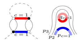
Figure 9: For $d=3$, $n_{e}^{(c=1)}$ is shown above in colored (left) and stranded (right) representations. $\{p\}=\{p_{1},p_{2},p_{3}\}$ and ${|{\bf p}_{\check{c}}|}^{2b}={|p|}^{2b}+{|p_{2}|}^{2b}$.

The Feynman amplitude associated with the graph $n_{e}^{(c)}$ shown in Fig. 9 is

$$K_{n_{e}^{(c)}}S_{n_{e}^{(c)}}(\{p\}) = 2\Big{(}-\frac{{\lambda_{\times}}^{(c)}}{2}\Big{)}|p_{c}|^{2a}\sum_{q_{c}}\frac{|q_{c}|^{2a}}{(|q_{c}|^{2b}+{|{\bf p}_{\check{c}}|}^{2b}+\mu)}\,,$$ (185)

where $K_{n_{e}^{(c)}}=2$.

Let us now compute the renormalization of $Z_{a}$, up to first order in perturbation theory

$$|p_{c}|^{2a}\Gamma_{2;a}(\{p\}) = -|p_{c}|^{2a}Z_{a}^{(c)}+K_{n_{e}^{(c)}}S_{n_{e}^{(c)}}(\{p\})$$ (186)

$$= -|p_{c}|^{2a}Z_{a}^{(c)}-\lambda_{\times}^{(c)}|p_{c}|^{2a}\sum_{q_{c}}\frac{|q_{c}|^{2a}}{(|q_{c}|^{2b}+{|{\bf p}_{\check{c}}|}^{2b}+\mu)}\,.$$

Therefore, to the first order in perturbation,

$$Z_{a,{\rm ren}}^{(c)} = -\Gamma_{2;a}^{(c)}(\{p\})\big{|}_{\{p\}=0}=Z_{a}^{(c)}+\lambda_{\times}^{(c)}\sum_{q}\frac{|q|^{2a}}{|q|^{2b}+\mu}\,.$$ (187)

By imposing the color independence, we write

$$Z_{a,{\rm ren}}=Z_{a}+\lambda_{\times}\,S_{2}\,,$$ (188)

where $S_{2}$ is given in (131). In multiscale analysis, we write

$$Z_{a,i-1}=Z_{a,i}+\lambda_{\times,i}\,S_{2,i}\,,$$ (189)

where $S_{2,i}$ is given in (133).

We approximate $S_{2,i}$ in (A.53). Now, we use the fact that $Z_{a}$ has scaling dimension $\{Z_{a}\}=1$, and that $\lambda_{\times}$ does not run, and express the $\beta$-function of the coupling $Z_{a}$ as:

$$-(Z_{a,i-1}-Z_{a,i}) = \frac{\partial Z_{a,i}}{\partial i}=-\widetilde{S}_{2,i}\,\lambda_{\times,i}\,,$$ (190)

$$\frac{\partial Z_{a,i}}{\partial((\log M)i)} = \partial_{t}Z_{a}(t)=-\beta_{Z_{a}}\,\lambda_{\times}\,,$$ (191)

$$\beta_{Z_{a}} = \frac{\widetilde{S}_{2,i}}{\log M}=2>0\,,$$ (192)

where $\widetilde{S}_{2,i}$ is given in (A.53). Given the scaling dimension $\{Z_{a}\}=1$, and after fixing an initial condition at some $t_{0}$, the dimensionless solution of the above equation is straightforward:

$$\widetilde{Z}_{a}(t) = c_{0}e^{-t}(-\beta_{Z_{a}}\,\lambda_{\times}t+c_{4})$$ (193)

$$= -c_{0}\beta_{Z_{a}}\,\lambda_{\times}(t-t_{0})e^{-t}+\widetilde{Z}_{a}(t_{0})e^{-(t-t_{0})}\,.$$ (194)

In the UV, $t\to\infty$, the 2-point coupling $Z_{a}$ in the model $\times$ flows to 0.

4.4 Computing of $\Gamma_{2;2a}$ and $Z_{2a}$ RG equation

We focus on the RG flow for $Z_{2a}$. We denote by $|p_{c}|^{4a}\Gamma_{2;2a}^{(c)}(\{p\})$ the sum is over all amputated 1PI 2-point graphs at 1-loop whose boundaries follow the pattern of ${\rm Tr}_{2;c}({p}^{4a}\phi^{2})$.

The diagrams that will contribute at 1-loop are denoted $m_{ee}^{(c)}$ and depicted in Fig. 10. (Higher order diagrams are listed in Appendix C) For $m_{ee}^{(c)}$, $\omega_{d;\times}(m_{ee}^{(c)})=0$ and belongs to the class II in Table 2.

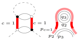
Figure 10: $m_{ee}^{(c=1)}$ for $d=3$ is illustrated in colored (left) and stranded (right) representations. $\{q_{\check{c}}\}=\{q_{2},\;q_{3}\}$, ${|{\bf q}_{\check{c}}|}^{2b}={|q_{2}|}^{2b}+{|q_{3}|}^{2b}$.

$$K_{m_{ee}^{(c)}}S_{m_{ee}^{(c)}}(\{p\}) = 2\Big{(}-\frac{{\lambda_{\times}}^{(c)}}{2}\Big{)}|p_{c}|^{4a}\sum_{\{q_{\check{c}}\}}\frac{1}{({|{\bf q}_{\check{c}}|}^{2b}+|p_{c}|^{2b}+\mu)}\,,$$ (195)

where $K_{m_{ee}^{(c)}}=2$. Given this, we compute the renormalization of $Z_{2a}$: where

$$|p_{c}|^{4a}\Gamma_{2;2a}^{(c)}\big{(}\{p\}) = -|p_{c}|^{4a}Z_{2a}^{(c)}+K_{m_{ee}^{(c)}}S_{m_{ee}^{(c)}}(\{p\})$$ (196)

$$= -|p_{c}|^{4a}Z_{2a}^{(c)}-{\lambda_{\times}}^{(c)}|p_{c}|^{4a}\sum_{\{q_{\check{c}}\}}\frac{1}{({|{\bf q}_{\check{c}}|}^{2b}+|p_{c}|^{2b}+\mu)}\,.$$

After a small manipulation, we obtain

$$Z_{2a,{\rm ren}}^{(c)} = Z_{2a}^{(c)}+{\lambda_{\times}}^{(c)}\sum_{\{q_{\check{c}}\}}\frac{1}{({|{\bf q}_{\check{c}}|}^{2b}+\mu)}\,.$$ (197)

The equation for $Z_{2a}$ is reached after requiring color independence:

$$Z_{2a,{\rm ren}}=Z_{2a}+\lambda_{\times}\,S_{1}\,,$$ (198)

where we recognize $S_{1}$ (131). Passing through the same steps via multiscale regularization, the coupling equation can be written as:

$$Z_{2a,i-1} = Z_{2a,i}+\lambda_{\times,i}\,S_{1,i}\,,$$ (199)

$$-(Z_{2a,i-1}-Z_{2a,i}) = \frac{\partial Z_{2a,i}}{\partial i}=-\,\widetilde{S}_{1,i}\,\lambda_{\times,i}\,,$$ (200)

$$\frac{\partial Z_{2a,i}}{\partial((\log M)i)} = \partial_{t}Z_{2a}(t)=-\beta_{Z_{2a}}\,\lambda_{\times}\,,$$ (201)

$$\beta_{Z_{2a}} = \frac{\widetilde{S}_{1,i}}{\log M}=2\pi>0\,,$$ (202)

where $\widetilde{S}_{1,i}$ is computed in (A.56). Then, because both couplings $Z_{2a}$ and $\lambda_{\times}$ are dimensionless, at this order of perturbation, $Z_{2a}$ yields also a linear function in the time scale $t$.

$$Z_{2a}(t) = -(t-t_{0})\,\beta_{Z_{2a}}\,\lambda_{\times}+Z_{a}(t_{0})\,.$$ (203)

The 2-point coupling $Z_{2a}$ in the model $\times$ grows linearly in $t$ in its magnitude. This behavior prevents one to conclude that the model is asymptotically safe. As commented before, the model is neither asymptotically free nor asymptotically safe which makes it interesting to understand better.

Summary – We give a summary of the 1-loop RG flow equations for the model $\times$ and their solutions, up to integration constants:

$\partial_{t}\widetilde{\lambda}=-2\widetilde{\lambda}$	$\widetilde{\lambda}(t)=c_{1}e^{-2t}$
$\partial_{t}\,\lambda_{\times}=0$	$\lambda_{\times}(t)=c_{2}$
$\partial_{t}\,\widetilde{\mu}=-2\widetilde{\mu}-\beta_{\mu,1}\widetilde{\lambda}$ ,   $\beta_{\mu,1}=2d\pi>0$	$\widetilde{\mu}(t)=(-\beta_{\mu,1}c_{1}t+c_{3})e^{-2t}$
$\partial_{t}\,\widetilde{Z}_{a}=-\widetilde{Z}_{a}-c_{0}e^{-t}\beta_{Z_{a}}\,\lambda_{\times}$ ,   $\beta_{Z_{a}}=2>0$	$\widetilde{Z}_{a}(t)=c_{0}(-\beta_{Z_{a}}\,\lambda_{\times}t+c_{4})e^{-t}$
$\partial_{t}\,Z_{2a}=-\beta_{Z_{2a}}\,\lambda_{\times}$  ,   $\beta_{Z_{2a}}=2\pi>0$	$Z_{2a}(t)=-\beta_{Z_{2a}}\,\lambda_{\times}t+c_{5}$

Table 4: Summary of the RG flow equations for the couplings in the model $\times$.

4.5 Integration at arbitrary loops

The power counting of the model $\times$ is provided by Proposition 2. This gives us more information on the $\beta$-functions of the couplings at arbitrary order of perturbation theory. Indeed, the information is stringent enough to let us present explicit general forms of $\beta$-functions of the couplings.

4-point couplings $\lambda$ and $\lambda_{\times}$ RG equation – The power counting theorem of the model $\times$ with Proposition 2 determines that at all orders in perturbation theory, there are no amplitudes which are divergent contributing to the renormalization of 4-point couplings $\lambda$ and $\lambda_{\times}$. Hence, $\lambda$ and $\lambda_{\times}$ of the model $\times$ are constant and therefore

$$\partial_{t}\lambda=0\;,\qquad\;\partial_{t}\lambda_{\times}=0\,,$$ (204)

which trivially yield, for the dimensionless coupling:

$$\widetilde{\lambda}(t)=c_{1}e^{-2t}\;,\qquad\;\lambda_{\times}(t)=c_{2}\,.$$ (205)

Mass, 2-point couplings $Z_{a}$ and $Z_{2a}$ RG equations – Observation of Proposition 2 tells us that the mass renormalization is decided by the class III, where only exactly one $\lambda$ and a number of $\lambda_{\times}$ contribute. The $Z_{a}$ renormalization is decided by the class I, where only $\lambda_{\times}$ contributes. We also notice that only $\lambda_{\times}$ contributes to the renormalization of $Z_{2a}$, as class II dictates.

With (205), one immediately conclude that the coupled differential RG equations for the couplings of the model $\times$, which generalize trivially the equations for the first order RG equations (180), (192), and (202), to arbitrary $n$-th orders, by introducing polynomials $P_{n}(\lambda_{\times})$, $Q_{n}(\lambda_{\times})$, and $R_{n}(\lambda_{\times})$, are

$$\partial_{t}\mu=\lambda\,P_{n}(\lambda_{\times})\,,\qquad\partial_{t}\widetilde{\mu}=-2\widetilde{\mu}+\widetilde{\lambda}\,P_{n}(\lambda_{\times})\,,$$ (206)

$$\partial_{t}Z_{a}=Q_{n}(\lambda_{\times})\,,\qquad\partial_{t}\widetilde{Z}_{a}=-\widetilde{Z}_{a}+e^{-t}Q_{n}(\lambda_{\times})\,,$$ (207)

$$\partial_{t}Z_{2a}=R_{n}(\lambda_{\times})\,,$$ (208)

which can be integrated easily. Thus each coupling will keep its behavior at arbitrary order of perturbation.

5 Conclusion

We have explicitly computed the one-loop $\beta$-functions of the couplings of two eTFTs, the model $+$ and the model $\times$, at first order of perturbation theory. The system of RG flow equations can be explicitly solved. Both models $+$ and $\times$ do have a constant wave function renormalization ($Z_{b}=1$). Nevertheless, we have obtained some nontrivial RG flows of the couplings. Table 3 and Table 4 summarize the upshot of this analysis.

For the model $+$, the enhanced $4$-point coupling $\lambda_{+}$ is marginal but without corrections; therefore it is a fixed point $\lambda_{+}=\theta$. Meanwhile, the ordinary $4$-point coupling $\lambda$ is relevant and therefore exponentially suppressed at large time $t=\log k/k_{0}$, where $k$ is momentum scale. This statement is true for all orders in perturbation theory. The 2-point coupling $Z_{a}$ and mass coupling have exponential behavior in $t$: they are suppressed in the UV and reach a constant. This is common for relevant operators. As a result, the current eTFT model $+$ behaves like an asymptotically safe model: one marginal direction $\lambda_{+}=\theta$ is kept fixed and there are three relevant operators $(\lambda,\mu,Z_{a})$ with dimensionless counterparts $(\widetilde{\lambda},\widetilde{\mu},\widetilde{Z}_{a})$ flowing to $(0,0,c\,\theta)$. This a one-dimensional line of fixed points that makes such a QFT interesting and special.

Concerning the model $\times$, the $4$-point coupling $\lambda_{\times}$ is marginal with no corrections: it becomes constant at all orders of perturbation and a fixed point, $\lambda_{\times}=\theta$. The second $4$-point coupling $\lambda$ is relevant but it is without corrections: it is exponentially suppressed towards the UV. On the other hand, the 2-point couplings, the mass and $Z_{a}$, are relevant and UV suppressed (they flow to 0). The last coupling $Z_{2a}$ is marginal and grows in its magnitude linearly in the scale $t$ with coefficient depending on $\lambda_{\times}=\theta$. We obtain the UV-behavior the dimensionless couplings $(\widetilde{\lambda},\widetilde{\mu},\widetilde{Z}_{a},Z_{2a})$ leads us to $(0,0,0,\infty)$. This behavior is not common of ordinary QFT and TFT as it cannot be associated neither with asymptotic freedom nor with asymptotic safety. Finally, comparing the RG flow equations between the conventional models and these eTFT, $+$ or $\times$ models, shows drastic differences. In the present context, they are simple enough to exhibit explicit solutions.

With the explicit forms of the running of the couplings at first order, together with the close observations of the power counting theorems for each model, $+$ or $\times$, in [35], we have deduced the generic form of the coupling $\beta$-functions at all orders of perturbation. The determination of the polynomial coefficients at all-loops will be left for future investigations. We conjecture that the systems could be explicitly integrated at arbitrary and given order. More generally, the amplitudes might be simple enough to be re-summed at all orders. Proving this property will require more work.

Concerning the quantum gravity side, the model $+$ can be called asymptotically safe at first order of perturbation for generic $\lambda_{+}$ and makes the UV completion of the quartic eTFTs likely. However, much less is known about its IR behavior. The computation of higher order perturbations of the models $+$ and $\times$ may reveal IR fixed points. Flowing backwards in the IR direction, the system of $\beta$-function collects polynomial coefficients in the coupling $\lambda_{+}$. The root of these polynomials may lead to vanishing $\beta$-functions and hence may produce non trivial IR fixed points. The IR study of eTFTs will require the use of different tools (like the Functional Renormalization Group Equation) and even different covariance with $p^{2a}$ weight. This could be also a following-up study from our work.

6 Acknowledgements

We thank anonymous referees for their reading and remarks that has led to corrections and radical improvement of our original work. We would like to thank Dario Benedetti, Sylvain Carrozza, Riccardo Martini, and Fabien Vignes-Tourneret for the insightful discussions. The authors would also like to thank the thematic program “Quantum Gravity, Random Geometry, and Holography” 9 January - 17 February 2023 at Institut Henri Poincaré, Paris, France for the platform for discussions and the collaboration and letting us progress further on this project. The authors acknowledge support of the Institut Henri Poincaré (UAR 839 CNRS-Sorbonne Université) and LabEx CARMIN (ANR-10-LABX-59-01).

Appendix

Appendix A Euler-Maclaurin formula and Feynman amplitude approximations

We briefly review the approximation of a discrete spectral sum by an integral using Euler-Maclaurin formula [23]. In perturbation theory, this approximation is well controlled and sufficient to achieve our calculations.

Consider $h_{n}(x)=x^{n}e^{-Ax^{a}}$, with $x\geq 0$, $n\in{\mathbbm{N}}$, and the sum $\sum_{p=0}^{\infty}h_{n}(p)$. We use Euler-Maclaurin formula to obtain for a finite integer $q\leq 1$,

$$\sum_{p=1}^{q}h_{n}(p)=\int_{1}^{q}h_{n}(p)dp+R(q)\,,$$ (A.1)

where

$$R(q)=-B_{1}\big{(}h_{n}(1)+h_{n}(q)\big{)}+\sum_{k=1}^{\infty}\frac{B_{2k}}{2k!}\big{(}h_{n}^{(2k-1)}(q)-h_{n}^{(2k-)}(1)\big{)}\,,$$ (A.2)

where $B_{k}$ are Bernoulli numbers and $h^{(2k-1)}$ denotes $2k-1^{\rm th}$ derivative of $h_{n}(p)$ with respect to $p$.

One can show that

$${\rm lim}_{q\rightarrow\infty}R(q)=-B_{1}-\sum_{k=1}^{\infty}\frac{B_{2k}}{2k}\binom{n}{2k-1}+{\mathcal{O}}(A)={\mathcal{O}}(1)+{\mathcal{O}}(A)\,.$$ (A.3)

For any $A$, the integral below is exact,

$${\rm lim}_{q\rightarrow\infty}\int_{1}^{q}h_{n}(p)dp=\frac{1}{a}A^{-\frac{1+n}{a}}\Gamma\Big{[}\frac{1+n}{a},A\Big{]}=\frac{1}{a}A^{-\frac{1+n}{a}}\Gamma\Big{[}\frac{1+n}{a}\Big{]}-\frac{1}{1+n}+{\mathcal{O}}(A)\,,$$ (A.4)

with the incomplete Gamma function $\Gamma[\cdot,\cdot]$, and Euler Gamma function $\Gamma[\cdot]$. This then gives us

$$\sum_{p=1}^{\infty}h_{n}(p)={\rm lim}_{q\rightarrow\infty}\sum_{p=1}^{q}h_{n}(p)=\frac{1}{a}A^{-\frac{1+n}{a}}\Gamma\Big{[}\frac{1+n}{a}\Big{]}-\frac{1}{1+n}+{\mathcal{O}}(1)+{\mathcal{O}}(A)\,.$$ (A.5)

Expanding $\widetilde{S}_{0,i}$. The goal is to approximate $S_{0,i}$ (98) using the above developments. Use Euler-Maclaurin expansion, we compute the sum

$$\tilde{\tau} = \sum_{q\in{\mathbbm{Z}}}|q|^{4a}e^{-(\alpha+\alpha^{\prime})|q|^{2b}}=2\sum_{q=1}^{\infty}q^{4a}e^{-(\alpha+\alpha^{\prime})|q|^{2b}}$$ (A.8)

$$=2\int_{1}^{\infty}dq\,q^{4a}e^{-(\alpha+\alpha^{\prime})|q|^{2b}}+R=2\times\frac{1}{2b(\alpha+\alpha^{\prime})^{\frac{4a+1}{2b}}}\Gamma\left(\frac{4a+1}{2b},\alpha+\alpha^{\prime}\right)+R$$

$$=\frac{(\alpha+\alpha^{\prime})^{\frac{-(4a+1)}{2b}}}{b}\Gamma\left(\frac{4a+1}{2b},\alpha+\alpha^{\prime}\right)+R\,,$$

where $\Gamma(s,x)=\int_{x}^{\infty}t^{s-1}e^{-t}dt$ denotes the upper incomplete Gamma function. $R$ is the Euler-Maclaurin remainder which behaves, according to (A.5), as $R={\mathcal{O}}(1)+{\mathcal{O}}(\alpha+\alpha^{\prime})$. $\Gamma(s,x)$ admits a known asymptotic expansion when $x\to 0^{+}$ given by

$$\Gamma(s,x)=\Gamma(s)-\frac{x^{s}}{s}+{\mathcal{O}}(x^{s+1})$$ (A.9)

with the obstruction $s\notin\{0,-1,-2,\dots\}$. Now, for simplicity, we constrain our model and use $D=1$, but keep $a$ and $b$ accordingly as given by Theorem 1. We use the above expansion (A.9) in (A.8) as $\alpha+\alpha^{\prime}$ is a small parameter (recalling that $\alpha$ and $\alpha^{\prime}$ are small in the UV)

$$\sum_{q\in{\mathbbm{Z}}}|q|^{4a}e^{-(\alpha+\alpha^{\prime})|q|^{2b}}$$ (A.10)

$$=\frac{(\alpha+\alpha^{\prime})^{\frac{-(4a+1)}{2b}}}{b}\left(\Gamma\left(\frac{4a+1}{2b}\right)-\frac{(\alpha+\alpha^{\prime})^{\frac{4a+1}{2b}}}{\frac{4a+1}{2b}}+{\mathcal{O}}\big{(}(\alpha+\alpha^{\prime})^{\frac{4a+1}{2b}+1}\big{)}\right)+R$$ (A.11)

$$=\frac{1}{b}\Gamma\left(\frac{4a+1}{2b}\right)(\alpha+\alpha^{\prime})^{\frac{-(4a+1)}{2b}}+{\mathcal{O}}(1)+{\mathcal{O}}(\alpha+\alpha^{\prime})\,.$$ (A.12)

Having a look at (98), using $e^{-(\alpha+\alpha^{\prime})\mu}=1+{\mathcal{O}}(\alpha+\alpha^{\prime})$, we integrate this expression above over $\alpha$ and $\alpha^{\prime}$, with $\frac{1}{b}\Gamma\left(\frac{4a+1}{2b}\right)=\frac{1}{b}\Gamma(2)=\frac{1}{b}$, and write:

$$\widetilde{S}_{0,i} = \int_{M^{-2bi}}^{M^{-2b(i-1)}}d\alpha\int_{M^{-2bi}}^{M^{-2b(i-1)}}d\alpha^{\prime}\Big{[}\frac{1}{b}(\alpha+\alpha^{\prime})^{-2}+{\mathcal{O}}\big{(}(\alpha+\alpha^{\prime})^{-1}\big{)}\Big{]}$$ (A.13)

$$= \int_{M^{-2bi}}^{M^{-2b(i-1)}}d\alpha\Big{[}-\frac{1}{b}(\alpha+\alpha^{\prime})^{-1}+{\mathcal{O}}\big{(}\log(\alpha+\alpha^{\prime})\big{)}\Big{]}_{\alpha^{\prime}=M^{-2bi}}^{\alpha^{\prime}=M^{-2b(i-1)}}$$ (A.14)

$$= \frac{1}{b}\Big{[}\log(\alpha+M^{-2bi})-\log(\alpha+M^{-2b(i-1)})$$ (A.16)

$$+\Big{(}\;{\mathcal{O}}\big{(}\alpha)+{\mathcal{O}}\big{(}\alpha\log(\alpha+M^{-2bi})\big{)}+{\mathcal{O}}\big{(}M^{-2bi}\log(\alpha+M^{-2bi})\big{)}\Big{)}\Big{]}_{\alpha=M^{-2bi}}^{\alpha=M^{-2b(i-1)}}$$

$$= \frac{1}{b}\Big{[}-\log(2M^{-2bi})+2\log(M^{-2b(i-1)}+M^{-2bi})-\log(2M^{-2b(i-1)})$$ (A.18)

$$+\;{\mathcal{O}}\big{(}M^{-2bi})+{\mathcal{O}}\big{(}M^{-2bi}\log(M^{-2bi})\big{)}\Big{]}$$

$$= \frac{1}{b}\Big{[}2\log[M^{-2bi}(M^{2b}+1)]-\log(2M^{-2bi})-\log(2M^{-2bi+2b})\Big{]}$$ (A.20)

$$+{\mathcal{O}}(M^{-2bi})+{\mathcal{O}}\big{(}M^{-2bi}\log(M^{-2bi})\big{)}$$

$$= \frac{1}{b}\Big{[}2\log(M^{2b}+1)-\log(4)-\log(M^{2b})\Big{]}+{\mathcal{O}}(M^{-2bi})+{\mathcal{O}}\big{(}M^{-2bi}\log(M^{-2bi})\big{)}$$ (A.22)

$$= \frac{1}{b}\Big{[}\log\frac{(M^{2b}+1)^{2}}{4M^{2b}}\Big{]}+{\mathcal{O}}(M^{-2bi})+{\mathcal{O}}\big{(}M^{-2bi}\log(M^{-2bi})\big{)}$$ (A.23)

Thus $\widetilde{S}_{0,i}$ is approximated by

$$\widetilde{S}_{0,i}=\frac{1}{b}\log\frac{(M^{2b}+1)^{2}}{4M^{2b}}+{\mathcal{O}}(M^{-2bi}\log(M^{-2bi}))$$ (A.25)

As $M\geq 1$, $\frac{(M^{2b}+1)^{2}}{(4M^{2b})}>1$, then the leading coefficient in the above expanding is positive.

We can put the above in a standard $\log M$ approximation by expanding at large enough $M\gg 1$:

$$\frac{1}{b}\log\frac{(M^{2b}+1)^{2}}{(4M^{2b})}=\frac{1}{b}\Big{[}\log(M^{2b})+2\log(1+1/M^{2b})-\log(4)\Big{]}$$ (A.26)

$$=\frac{1}{b}\log M^{2b}+\frac{2}{b}\left(\frac{1}{M^{2b}}-\log(2)\right)+{\mathcal{O}}(M^{-4b})$$ (A.27)

At large $M$, the first term will correspond to the standard $\log\Lambda$ divergence for marginal coupling.

Dimensionful computations for $S_{0,i}$. We address now the crucial question of the dimension in our computation. The previous calculations of were performed without taking care of that aspect that we now restore. The couplings and fields have scaling dimensions. Expressing the propagator in Schwinger parameterization as in (65), we notice that $\alpha$ should have a dimension of $-2b$ in units of momentum scale $k$. In other words, we can write $\alpha=k^{-2b}\,{\tilde{\alpha}}$ where ${\tilde{\alpha}}$ is dimensionless. There is a dimensionful quantity $\tau$ associated with $\tilde{\tau}$ (A.8), in which $q$ acquires dimension of $1$ in the units of the momentum scale. The integral approximates the discrete sum over $q$ as in the second line of (A.8), but gains one more dimension in the computation of $\tau$. A similar fact concerning discrete sums having scaling dimensions was advocated and used in [32]. This also can be understood by the power counting theorem: in order to make the couplings marginal, so $\log$-divergent in the cut-off, discrete sums must carry scale dimension. We perform the following change of variables to let the dimensions be explicit in terms of a momentum scale $k$:

$$q=k\tilde{q}\,,\qquad\tilde{q}\in{\mathbbm{Z}}$$ (A.28)

$$\alpha=k^{-2b}\,{\tilde{\alpha}}$$ (A.29)

We obtain in terms of dimensionless $\tilde{\tau}$ and $\widetilde{S}_{0,i}$:

$$\tau=k^{4a+1}\tilde{\tau}$$ (A.30)

$$S_{0,i}=k^{4a+1}k^{-4b}\widetilde{S}_{0,i}=\widetilde{S}_{0,i}\,,$$ (A.31)

where in the last equality, we notice $4a+1-4b=0$, and therefore we get $S_{0,i}$ (101).

Expanding $\widetilde{S}_{1,i}$ and $\widetilde{S}_{2,i}$ for model $+$. We use a similar technique to provide an approximation of $S_{1,i}$ (132) and $S_{2,i}$ (133).

Express the propagators in Schwinger representation and carefully converting the above sums into integrals and get

$$\widetilde{S}_{2,i}=\int_{0}^{\infty}d\alpha\chi^{i}(\alpha)e^{-\alpha\mu_{i}}\sum_{q\in{\mathbbm{Z}}}|q|^{2a}e^{-\alpha|q|^{2b}}\,.$$ (A.32)

This integral is similar to (A.8), changing only $\alpha+\alpha^{\prime}$ to $\alpha$ and for a particular choice of $2a$. We perform an approximation in an analogous manner as before and get:

$$\sum_{q\in{\mathbbm{Z}}}|q|^{2a}e^{-\alpha|q|^{2b}}=\frac{\alpha^{\frac{-(2a+1)}{2b}}}{b}\Gamma\left(\frac{2a+1}{2b},\alpha\right)+R=\frac{1}{b}\Gamma\left(\frac{2a+1}{2b}\right)\alpha^{\frac{-(2a+1)}{2b}}+{\mathcal{O}}(1)$$ (A.33)

We insert this expression in (A.32) and obtain

$$\widetilde{S}_{2,i} = \int_{M^{-2bi}}^{M^{-2b(i-1)}}d\alpha e^{-\alpha\mu_{i}}\Big{[}c_{1;a,b}\,\alpha^{\frac{-(2a+1)}{2b}}+{\mathcal{O}}(1)\Big{]}$$ (A.34)

$$= \int_{M^{-2bi}}^{M^{-2b(i-1)}}d\alpha(1+{\mathcal{O}}(\alpha))\Big{[}c_{1;a,b}\,\alpha^{\frac{-(2a+1)}{2b}}+{\mathcal{O}}(1)\Big{]}$$ (A.35)

$$= \int_{M^{-2bi}}^{M^{-2b(i-1)}}d\alpha\Big{[}c_{1;a,b}\,\alpha^{\frac{-(2a+1)}{2b}}+{\mathcal{O}}\big{(}\alpha^{1-\frac{(2a+1)}{2b}}\big{)}\Big{]}$$ (A.36)

$$= \Big{[}\frac{1}{1-\frac{(2a+1)}{2b}}\,c_{1;a,b}\,\alpha^{1-\frac{(2a+1)}{2b}}+{\mathcal{O}}\big{(}\alpha^{2-\frac{(2a+1)}{2b}}\big{)}\Big{]}_{M^{-2bi}}^{M^{-2b(i-1)}}\,,$$ (A.37)

where $c_{1;a,b}=\frac{1}{b}\Gamma\left(\frac{2a+1}{2b}\right)$.

For the model $+$, we use $a=\frac{1}{2}D(d-2)$ and $b=\frac{1}{2}D(d-\frac{3}{2})$ for just-renormalizability (see Proposition 1) with $D=1$, then, $\frac{2a+1}{2b}=\frac{2(d-1)}{2d-3}=1+\frac{1}{2d-3}$. Thus

$$\widetilde{S}_{2,i} = \Big{[}-\frac{(2d-3)}{(2d-3)/4}\,\Gamma\left(\frac{2(d-1)}{2d-3}\right)\alpha^{-1/(2d-3)}+{\mathcal{O}}\big{(}\alpha^{1-1/(2d-3)}\big{)}\Big{]}_{M^{-2bi}}^{M^{-2b(i-1)}}$$ (A.38)

$$= 4\,\Gamma\Big{(}\frac{2(d-1)}{2d-3}\Big{)}(M^{-2bi(-1/4b)}-M^{-2b(i-1)(-1/4b)})+{\mathcal{O}}\big{(}M^{-i(d-2)}\big{)}$$ (A.39)

$$= 4\,\Gamma\Big{(}\frac{2(d-1)}{2d-3}\Big{)}M^{i/2}(1-M^{-1/2})+{\mathcal{O}}\big{(}M^{-i(d-2)}\big{)}\,.$$ (A.40)

Now we compute $\widetilde{S}_{1,i}$ namely,

$$\widetilde{S}_{1,i}=\sum_{{\bf q}\in{\mathbbm{Z}}^{d-1}}\int_{0}^{\infty}d\alpha\;\chi^{i}(\alpha)\,e^{-\alpha(|{\bf q}|^{2b}+\mu_{i})}=\int_{0}^{\infty}d\alpha\chi^{i}(\alpha)e^{-\alpha\mu_{i}}\left(\sum_{q\in{\mathbbm{Z}}}e^{-\alpha|q|^{2b}}\right)^{d-1}\,.$$ (A.41)

Let us focus on a single sum over $q$:

$$\sum_{q\in{\mathbbm{Z}}}e^{-\alpha|q|^{2b}}=2\sum_{q=1}^{\infty}e^{-\alpha q^{2b}}+1=2\int_{1}^{\infty}dqe^{-\alpha q^{2b}}+R+1$$ (A.42)

$$=2\Bigg{(}\frac{1}{2b}\alpha^{-\frac{1}{2b}}\Gamma\left(\frac{1}{2b},\alpha\right)\Bigg{)}+R+1\,,$$ (A.43)

where $R={\mathcal{O}}(1)+{\mathcal{O}}(\alpha)$. We use (A.9) in (A.43) as $\alpha$ is a small parameter in the UV,

$$\sum_{q\in{\mathbbm{Z}}}e^{-\alpha|q|^{2b}}=\frac{1}{b}\alpha^{-\frac{1}{2b}}\Big{[}\Gamma\left(\frac{1}{2b}\right)-2b\alpha^{\frac{1}{2b}}+{\mathcal{O}}(\alpha^{\frac{1}{2b}+1})\Big{]}+R+1=\frac{1}{b}\Gamma\left(\frac{1}{2b}\right)\alpha^{-\frac{1}{2b}}+{\mathcal{O}}(1)\,.$$ (A.44)

We insert this expression in (A.41),

$$\widetilde{S}_{1,i}=\int_{0}^{\infty}d\alpha\chi^{i}(\alpha)e^{-\alpha\mu_{i}}\left(\frac{1}{b}\Gamma\left(\frac{1}{2b}\right)\alpha^{-\frac{1}{2b}}+{\mathcal{O}}(1)\right)^{d-1}$$ (A.45)

$$= \int_{M^{-2bi}}^{M^{-2b(i-1)}}d\alpha\,e^{-\alpha\mu_{i}}\Big{[}\Bigg{(}\frac{1}{b}\Gamma\left(\frac{1}{2b}\right)\Bigg{)}^{d-1}\alpha^{-\frac{d-1}{2b}}+{\mathcal{O}}(\alpha^{-\frac{d-2}{2b}})\Big{]}$$ (A.46)

$$= \int_{M^{-2bi}}^{M^{-2b(i-1)}}d\alpha(1+{\mathcal{O}}(\alpha))\Big{[}\Bigg{(}\frac{1}{b}\Gamma\left(\frac{1}{2b}\right)\Bigg{)}^{d-1}\alpha^{-\frac{d-1}{2b}}+{\mathcal{O}}(\alpha^{-\frac{d-2}{2b}})\Big{]}$$ (A.47)

$$= \Big{[}\Bigg{(}\frac{1}{b}\Gamma\left(\frac{1}{2b}\right)\Bigg{)}^{d-1}\frac{1}{1-\frac{d-1}{2b}}\alpha^{1-\frac{d-1}{2b}}+{\mathcal{O}}(\alpha^{1-\frac{d-2}{2b}})\Big{]}_{M^{-2bi}}^{M^{-2b(i-1)}}$$ (A.48)

$$= \Bigg{(}\frac{1}{b}\Gamma\left(\frac{1}{2b}\right)\Bigg{)}^{d-1}\frac{2b}{2b-d+1}M^{-i(2b-d+1)}\Big{(}M^{(2b-d+1)}-1\Big{)}+{\mathcal{O}}(M^{-i(2b-d+2)})\,,\qquad$$ (A.49)

For the model $+$, we use $b=\frac{1}{2}D(d-\frac{3}{2})$ for just-renormalizability (see Proposition 1) with $D=1$, then:

$$\widetilde{S}_{1,i}=\Bigg{(}\frac{1}{b}\Gamma\left(\frac{1}{2b}\right)\Bigg{)}^{d-1}(2d-3)M^{i/2}\Big{(}1-M^{-1/2}\Big{)}+{\mathcal{O}}(M^{-i/2})\,.$$ (A.50)

$\widetilde{S}_{1,i}$ and $\widetilde{S}_{2,i}$ for the model $\times$. For the model $\times$, from the Proposition 2, we have a specific set of parameters, i.e., $D=1$, $d=3$, $a=\frac{1}{2}$, $b=1$, and $\frac{2a+1}{2b}=1$. We then specialize the previous computation. Starting from (A.35), we have

$$\widetilde{S}_{2,i} = \int_{M^{-2i}}^{M^{-2(i-1)}}d\alpha(1+{\mathcal{O}}(\alpha))\Big{[}\alpha^{-1}+{\mathcal{O}}(1)\Big{]}$$ (A.51)

$$= \Big{[}\log\alpha+{{\mathcal{O}}(\alpha)}\Big{]}_{M^{-2i}}^{M^{-2(i-1)}}$$ (A.52)

$$= 2\log M+{\mathcal{O}}(M^{-2(i-1)})\,.$$ (A.53)

For the model $\times$, from the Proposition 2, we have a specific set of parameters, i.e., $D=1$, $d=3$, $a=\frac{1}{2}$, $b=1$, and $\frac{d-1}{2b}=1$. So, recomputing (A.49), we get:

$$\widetilde{S}_{1,i} = \int_{M^{-2i}}^{M^{-2(i-1)}}d\alpha(1+{\mathcal{O}}(\alpha))\Big{[}\Big{(}\Gamma\left(\frac{1}{2}\right)\Big{)}^{2}\alpha^{-1}+{\mathcal{O}}(\alpha^{-\frac{1}{2}})\Big{]}$$ (A.54)

$$= \Big{[}\pi\log\alpha+{\mathcal{O}}(\alpha^{\frac{1}{2}})\Big{]}^{M^{-2(i-1)}}_{M^{-2i}}$$ (A.55)

$$= 2\pi\log M+{\mathcal{O}}\big{(}{M^{-i}}\big{)}\,,$$ (A.56)

where we substitute $\Gamma\left(\frac{1}{2}\right)=\sqrt{\pi}$.

Dimensionful computations of $S_{1,i}$ (132) and $S_{2,i}$ (133). Following the similar argument as for $S_{0,i}$, we perform the changes of variables given in (A.29) so that the dimensions are explicit in computations. Then, we obtain in terms of dimensionless $\widetilde{S}_{1,i}$ and $\widetilde{S}_{2,i}$:

$$S_{1,i}=k^{-2b}k^{d-1}\widetilde{S}_{1,i}$$ (A.57)

$$S_{2,i}=k^{-2b}\,k^{2a}\,k\widetilde{S}_{2,i}\,,$$ (A.58)

where in the last equalities, we note from Propositions 1 and 2 that

$$d-1-2b=2a-2b+1=\begin{cases}\frac{1}{2},&\text{for the model }+\\ 0,&\text{for the model }\times\end{cases}$$ (A.59)

Appendix B Higher order perturbation of model $+$

This appendix illustrates the higher order corrections of the different couplings RG flow. These manifestly highlight the structure of the RG flow at higher loops.

B.1 4-point function at third order

• The graph $n_{42}^{(c)}$ has degree of divergence $\omega_{n_{42}^{(c)}}=0$, following the first row of Table 1, and its amplitude appears at the third order in perturbation theory.

  

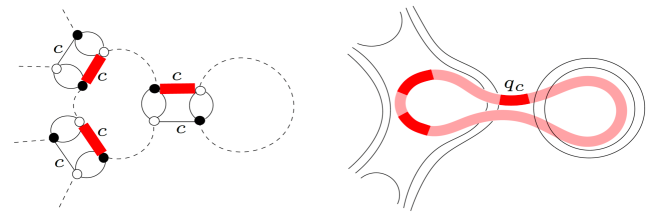
  Figure 11: A two-loop divergent graph, $n_{42}^{(c)}$ contributing to $\Gamma_{4}^{(c)}(\{p\})$, at $d=3$.

  Explicitly, at two-loop,

  $$K_{n_{42}^{(c)}}=12\,,$$ (B.60)

  $$S_{n_{42}^{(c)}}(\{\mathbf{p},\mathbf{p}^{\prime}\})=\frac{1}{3!}\Big{(}\frac{-\lambda^{(c)}_{+}}{2}\Big{)}^{3}\sum_{\{q\}}\frac{\big{(}|q_{c}|^{2a}\big{)}^{3}}{(|\mathbf{p}_{\check{c}}|^{2b}+|q_{c}|^{2b}+\mu)(|\mathbf{p}^{\prime}_{\check{c}}|^{2b}+|q_{c}|^{2b}+\mu)^{2}(|\mathbf{q}|^{2b}+\mu)}\,.$$

  The contribution to the Feynman amplitude will be of the form $\sum_{c}K_{n_{42}^{(c)}}S_{n_{42}^{(c)}}$.

B.2 $\Gamma_{2}$ at second order

The following graphs will contribute to the flow of the $Z_{a}$ coupling. Computing it, we distinguish the colors and introduce $Z_{a}^{(c)}$ which makes us work at fixed color $c$.

• For $m_{2e}^{(c\,c^{\prime})}$, $\omega_{m_{2e}^{(c\,c^{\prime})}}=0$. This graph belongs to the class V in Table 1.

  

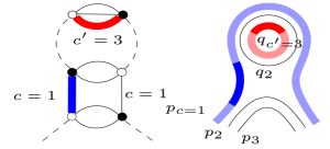
  Figure 12: The graph $m_{2e}^{(c=1\,c^{\prime}=2)}$, for $d=3$ is illustrated. $\{q_{\check{c}=\check{1}}\}=\{q_{c^{\prime}=2},\;q_{3}\}$, and ${|{\bf q}_{\check{1}}|}^{2b}={|q_{2}|}^{2b}+{|q_{3}|}^{2b}$.

  The contribution to the Feynman amplitude is then,

  $$\sum_{c^{\prime}}K_{m_{2e}^{(c\,c^{\prime})}}S_{m_{2e}^{(c\,c^{\prime})}}(\{p\}) = \sum_{c^{\prime}\neq c}^{(d-1)\;{\rm terms}}2\Big{[}\Big{(}-\frac{{\lambda_{+}}^{(c)}}{2}\Big{)}(-Z_{a}^{(c^{\prime})})\Big{]}\sum_{\{q_{\hat{c}}\}}\frac{{|q_{c^{\prime}}|}^{2a}{|p_{c}|}^{2a}}{({|{\bf q}_{{(\check{c})}}|}^{2b}+|{p_{c}|}^{2b}+\mu)^{2}}$$ (B.61)

  $$= \lambda_{+}^{(c)}{|p_{c}|}^{2a}\sum_{c^{\prime}\neq c}^{(d-1)\;{\rm terms}}Z_{a}^{(c^{\prime})}\sum_{\{q_{\check{c}}\}}\frac{{|q_{c^{\prime}}|}^{2a}}{({|{\bf q}_{{(\check{c})}}|}^{2b}+{|p_{c}|}^{2b}+\mu)^{2}}\,,$$

  where $K_{m_{2e}^{(c\,c^{\prime})}}=2$.

• The graph $meme_{2}^{(c\,c^{\prime})}$, is such that $\omega_{meme_{2}^{(c\,c^{\prime})}}=\frac{D}{2}$ and it appears in the class II in Table 1.

  

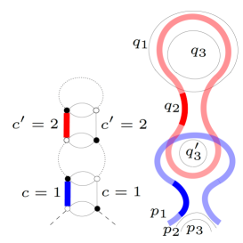
  Figure 13: For $d=3$, $meme_{2}^{(c=1\,c^{\prime}=2)}$ is illustrated. $q^{\prime}_{({\check{c}}{\check{c^{\prime}}})}={q^{\prime}}_{3}$, $\{q\}=\{q_{1},q_{2},q_{3}\}$, ${|{\bf q}|}^{2b}={|q_{1}|}^{2b}+{|q_{2}|}^{2b}+{|q_{3}|}^{2b}$, ${|{\bf q}_{({\check{c}}{\check{c^{\prime}}})}|}^{2b}={|q_{3}|}^{2b}$.

  $$\sum_{c^{\prime}\neq c}K_{meme_{2}^{(c,c^{\prime})}}S_{meme_{2}^{(c,c^{\prime})}}(\{p\})$$ (B.63)

  $$= \sum_{c^{\prime}\neq c}^{(d-1)\;{\rm terms}}K_{meme_{2}^{(c,c^{\prime})}}\Big{(}-\frac{\lambda_{+}^{(c)}}{2}\Big{)}\Big{(}-\frac{\lambda_{+}^{(c^{\prime})}}{2}\Big{)}{|p_{c}|}^{2a}$$

  $$\qquad\quad\sum_{\{q^{\prime}_{({\check{c}}{\check{c^{\prime}}})}\},\{q\}}\frac{{|q_{c^{\prime}}|}^{2a}}{({|{\bf q}|}^{2b}+\mu)({|{\bf q^{\prime}}_{({\check{c}}{\check{c^{\prime}}})}|}^{2b}+{|q_{c^{\prime}}|}^{2b}+{|p_{c}|}^{2b}+\mu)^{2}}$$

  where $K_{meme_{2}^{(c,c^{\prime})}}=4$, and where we introduced the notation $q^{\prime}_{({\check{c}}{\check{c^{\prime}}})}$ which means that the color of this momentum cannot be neither $c$ nor $c^{\prime}$.

B.3 Self energy and mass corrections

We gather here the contributions to the self-energy and wave function renormalization $Z_{b}$ at second order of perturbation.

• For the graph $m_{2}^{(c,c^{\prime})}$, the degree of divergence is given by $\omega_{d;+}(m_{2}^{(c,c^{\prime})})=0$. The class VI in Table 1 includes this graph.

  

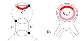
  Figure 14: $m_{2}^{(c,c^{\prime})}$ in colored and stranded representations at $d=3$. ${|{\bf q}_{\check{c}}|}^{2b}={|q_{c^{\prime}}|}^{2b}+{|q_{1}|}^{2b}$ and $\{q_{\check{c}}\}=\{q_{c^{\prime}},\;q_{1}\}$.

  The contribution of the graph $m_{2}^{(c,c^{\prime})}$ shown in Fig. 14 in the amplitude is

  $$\sum_{c,c^{\prime}\neq c}K_{m_{2}^{(c,c^{\prime})}}S_{m_{2}^{(c,c^{\prime})}}(\{p\}) = \sum_{c,c^{\prime}\neq c}^{d\times(d-1)\;{\rm terms}}2\Big{[}\Big{(}-\frac{\lambda^{(c)}}{2}\Big{)}\Big{(}-{Z_{a}}^{(c^{\prime})}\Big{)}\Big{]}\sum_{\{q_{\check{c}}\}}\frac{|q_{c^{\prime}}|^{2a}}{({|{\bf q}_{\check{c}}|}^{2b}+|p_{c}|^{2b}+\mu)^{2}}$$ (B.64)

  $$= \sum_{c=1}^{d}\lambda^{(c)}\sum_{c^{\prime}\neq c}\sum_{\{q_{\check{c}}\}}\frac{{Z_{a}}^{(c^{\prime})}|q_{c^{\prime}}|^{2a}}{({|{\bf q}_{\check{c}}|}^{2b}+|p_{c}|^{2b}+\mu)^{2}}\,,$$

  where $K_{m_{2}^{(c,c^{\prime}\neq c)}}=2$.

• Concerning the graph $mme_{2}^{(c,c^{\prime})}$, the superficial degree of divergence is $\omega_{d;+}(mme_{2}^{(c,c^{\prime})})=\frac{D}{2}$. It can be found in the class III in Table 1.

  

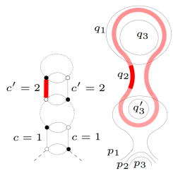
  Figure 15: $mme_{2}^{(c=1,c^{\prime}=2)}$, for $d=3$ in colored and stranded representations, with $q^{\prime}_{({\check{c}}{\check{c^{\prime}}})}={q^{\prime}}_{3}$, ${|{\bf q}_{({\check{c}}{\check{c^{\prime}}})}|}^{2b}={|q_{3}|}^{2b}$.

  The amplitude associated with the graph $mme_{2}^{(c,c^{\prime})}$ shown in Fig. 15 is given by

  $$\sum_{c,c^{\prime}\neq c}K_{mme_{2}^{(c,c^{\prime})}}S_{mme_{2}^{(c,c^{\prime})}}(\{p\})$$ (B.65)

  $$= \sum_{c,c^{\prime}\neq c}^{d\times(d-1)\;{\rm terms}}4\Big{[}\Big{(}-\frac{\lambda^{(c)}}{2}\Big{)}\Big{(}-\frac{\lambda_{+}^{(c^{\prime})}}{2}\Big{)}\Big{]}$$ (B.67)

  $$\qquad\qquad\sum_{\{q^{\prime}_{({\check{c}}{\check{c^{\prime}}})}\},\{q\}}\frac{{|q_{c^{\prime}}|}^{2a}}{({|{\bf q}|}^{2b}+\mu)({|{\bf q^{\prime}}_{({\check{c}}{\check{c^{\prime}}})}|}^{2b}+{|q_{c^{\prime}}|}^{2b}+{|p_{c}|}^{2b}+\mu)^{2}}$$

  $$= \sum_{c=1}^{d}\lambda^{(c)}\sum_{c^{\prime}\neq c}\sum_{\{q^{\prime}_{({\check{c}}{\check{c^{\prime}}})}\},\{q\}}\frac{\lambda_{+}^{(c^{\prime})}{|q_{c^{\prime}}|}^{2a}}{({|{\bf q}|}^{2b}+\mu)({|{\bf q^{\prime}}_{({\check{c}}{\check{c^{\prime}}})}|}^{2b}+{|q_{c^{\prime}}|}^{2b}+{|p_{c}|}^{2b}+\mu)^{2}}\,,\quad$$ (B.68)

  where $K_{mme_{2}^{(c,c^{\prime})}}=4$.

• For the graph $n_{2}^{(c)}$, $\omega_{d;+}(n_{2}^{(c)})=0$, and it belongs to the class IV in Table 1.

  

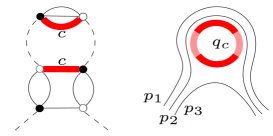
  Figure 16: The illustration of $n_{2}^{(c)}$ in $d=3$.

  Now the amplitude of $n_{2}^{(c)}$ is

  $$\sum_{c}K_{n_{2}^{(c)}}S_{n_{2}^{(c)}}(\{p\}) = \frac{1}{2}\sum_{c=1}^{d}{\lambda_{+}}^{(c)}Z_{a}^{(c)}\sum_{q_{c}}\frac{(|q_{c}|^{2a})^{2}}{(|q_{c}|^{2b}+{|{\bf p}_{\check{c}}|}^{2b}+\mu)^{2}}\,,$$ (B.69)

  where $K_{n_{2}^{(c)}}=1$.

• The $nme_{2}^{(c)}$ belongs to the class I in Table 1 and it fulfills $\omega_{d;+}(nme_{2}^{(c)})=\frac{D}{2}$.

  

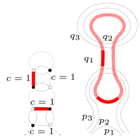
  Figure 17: For $d=3$, the $nme_{2}^{(c=1)}$ with ${|{\bf p}_{\check{c}}|}^{2b}={|p_{2}|}^{2b}+{|p_{3}|}^{2b}$.

  $$\sum_{c}K_{nme_{2}^{(c)}}S_{nme_{2}^{(c)}}(\{p\})$$ (B.70)

  $$= \sum_{c=1}^{d}4\frac{1}{2!}\Big{[}\Big{(}-\frac{{\lambda_{+}}^{(c)}}{2}\Big{)}^{2}\Big{]}\sum_{\{q\}}\frac{({|q_{c}|}^{2a})^{2}}{({|{\bf q}|}^{2b}+\mu)({|q_{c}|}^{2b}+{|{\bf p}_{\check{c}}|}^{2b}+\mu)^{2}}\,,$$ (B.71)

  $$= \frac{1}{2}\sum_{c=1}^{d}({\lambda_{+}}^{(c)})^{2}\sum_{\{q\}}\frac{({|q_{c}|}^{2a})^{2}}{({|{\bf q}|}^{2b}+\mu)({|q_{c}|}^{2b}+{|{\bf p}_{\check{c}}|}^{2b}+\mu)^{2}}\,,$$ (B.72)

  where $K_{nme_{2}^{(c)}}=4$.

Appendix C Second order perturbation of model $\times$

C.1 Self energy and mass corrections

• For $mm_{ee}^{(c,c^{\prime})}$, the superficial degree of divergence is $\omega_{d;\times}(mm_{ee}^{(c,c^{\prime})})=0$. This graph belongs to the class III in Table 2, and appears in the second order ${\mathcal{O}}(\lambda\,\lambda_{\times})$ in Taylor expansion.

  

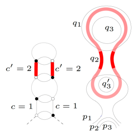
  Figure 18: $mm_{ee}^{(c=1,c^{\prime}=2)}$, for $d=3$ in both colored and stranded representations. $\{q^{\prime}_{({\check{c}}{\check{c^{\prime}}})}\}={q^{\prime}}_{3}$, ${|{\bf q}_{({\check{c}}{\check{c^{\prime}}})}|}^{2b}={|q_{3}|}^{2b}$.

  The amplitude associated with the graph $mm_{ee}^{(c,c^{\prime})}$ shown in Fig. 18 is given by

  $$\sum_{c,c^{\prime}\neq c}K_{mm_{ee}^{(c,c^{\prime})}}S_{mm_{ee}^{(c,c^{\prime})}}(\{p\})$$ (C.73)

  $$= \sum_{c,c^{\prime}\neq c}^{d\times(d-1)\;{\rm terms}}4\Big{[}\Big{(}-\frac{\lambda^{(c)}}{2}\Big{)}\Big{(}-\frac{\lambda_{\times}^{(c^{\prime})}}{2}\Big{)}\Big{]}$$ (C.75)

  $$\qquad\qquad\sum_{\{q^{\prime}_{({\check{c}}{\check{c^{\prime}}})}\},\{q\}}\frac{{|q_{c^{\prime}}|}^{4a}}{({|{\bf q}|}^{2b}+\mu)({|{\bf q^{\prime}}_{({\check{c}}{\check{c^{\prime}}})}|}^{2b}+{|q_{c^{\prime}}|}^{2b}+{|p_{c}|}^{2b}+\mu)^{2}}$$

  $$= \sum_{c=1}^{d}\lambda^{(c)}\sum_{c^{\prime}\neq c}\sum_{\{q^{\prime}_{({\check{c}}{\check{c^{\prime}}})}\},\{q\}}\frac{\lambda_{\times}^{(c^{\prime})}{|q_{c^{\prime}}|}^{4a}}{({|{\bf q}|}^{2b}+\mu)({|{\bf q^{\prime}}_{({\check{c}}{\check{c^{\prime}}})}|}^{2b}+{|q_{c^{\prime}}|}^{2b}+{|p_{c}|}^{2b}+\mu)^{2}}\,,$$ (C.76)

  where $K_{mm_{ee}^{(c,c^{\prime})}}=4$.

C.2 $\Gamma_{2;a}$ at second order

We work out the contribution to the flow of $Z_{a}^{(c)}$ at fixed color $c$.

• The graph $n_{ee}m_{ee}^{(c)}$ obeys $\omega_{d;\times}(n_{ee}m_{ee}^{(c)})=0$ and belongs to the class I in Table 2.

  

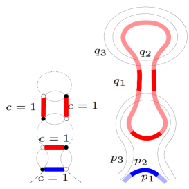
  Figure 19: The graph $n_{ee}m_{ee}^{(c=1)}$ at $d=3$. ${|{\bf p}_{\check{c}=\check{1}}|}^{2b}={|p_{2}|}^{2b}+{|p_{3}|}^{2b}$.

  $$K_{n_{ee}m_{ee}^{(c)}}S_{n_{ee}m_{ee}^{(c)}}(\{p\})$$ (C.77)

  $$= 8\,\frac{1}{2!}\Big{(}-\frac{{\lambda_{\times}}^{(c)}}{2}\Big{)}^{2}|p_{c}|^{2a}\sum_{\{q\}}\frac{({|q_{c}|}^{2a})^{3}}{({|{\bf q}|}^{2b}+\mu)({|q_{c}|}^{2b}+{|{\bf p}_{(\check{c})}|}^{2b}+\mu)^{2}}\,$$

  $$= {\lambda_{\times}}^{(c)}|p_{c}|^{2a}\sum_{\{q\}}\frac{({|q_{c}|}^{2a})^{3}}{({|{\bf q}|}^{2b}+\mu)({|q_{c}|}^{2b}+{|{\bf p}_{(\check{c})}|}^{2b}+\mu)^{2}}\,$$ (C.78)

  where we set $K_{n_{ee}m_{ee}^{(c)}}=8$.

C.3 $\Gamma_{2;2a}$ at second order

We list below the second order contributions to the flow of the last coupling $Z_{2a}^{(c)}$. We investigate this at given color $c$.

• The graph $m_{ee}m_{ee}^{(c,c^{\prime})}$ is part of the class II in Table 2. It has vanishing divergence degree: $\omega_{d;\times}(m_{ee}m_{ee}^{(c,c^{\prime})})=0$.

  

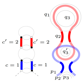
  Figure 20: The graph $m_{ee}m_{ee}^{(c=1,c^{\prime}=2)}$ illustrated at $d=3$. $q^{\prime}_{({\check{c}}{\check{c^{\prime}}})}={q^{\prime}}_{3}$, ${|{\bf q}_{({\check{c}}{\check{c^{\prime}}})}|}^{2b}={|q_{3}|}^{2b}$.

  $$\sum_{c^{\prime}\neq c}K_{m_{ee}m_{ee}^{(c,c^{\prime})}}S_{m_{ee}m_{ee}^{(c,c^{\prime})}}(\{p\})$$ (C.80)

  $$= \sum_{c^{\prime}\neq c}^{(d-1)\;{\rm terms}}4\Big{[}\Big{(}-\frac{\lambda_{\times}^{(c)}}{2}\Big{)}\Big{(}-\frac{\lambda_{\times}^{(c^{\prime})}}{2}\Big{)}\Big{]}{|p_{c}|}^{4a}$$

  $$\qquad\quad\sum_{\{q^{\prime}_{({\check{c}}{\check{c^{\prime}}})}\},\{q\}}\frac{{|q_{c^{\prime}}|}^{4a}}{({|{\bf q}|}^{2b}+\mu)({|{\bf q^{\prime}}_{({\check{c}}{\check{c^{\prime}}})}|}^{2b}+{|q_{c^{\prime}}|}^{2b}+{|p_{c}|}^{2b}+\mu)^{2}}$$

  $$= \lambda_{\times}^{(c)}{|p_{c}|}^{4a}\sum_{c^{\prime}\neq c}\sum_{\{q^{\prime}_{({\check{c}})}\},\{q\}}\frac{\lambda_{\times}^{(c^{\prime})}{|q_{c^{\prime}}|}^{4a}}{({|{\bf q}|}^{2b}+\mu)({|{\bf q^{\prime}}_{({\check{c}}{\check{c^{\prime}}})}|}^{2b}+{|q_{c^{\prime}}|}^{2b}+{|p_{c}|}^{2b}+\mu)^{2}}\,,\quad$$ (C.81)

  where $K_{m_{ee}m_{ee}^{(c,c^{\prime})}}=4$.

References

- [1] P. Di Francesco, P. H. Ginsparg and J. Zinn-Justin, “2-D Gravity and random matrices,” Phys. Rept. 254, 1 (1995) [arXiv:hep-th/9306153].
- [2] V. G. Knizhnik, A. M. Polyakov and A. B. Zamolodchikov, Mod. Phys. Lett. A 3, 819 (1988).
- [3] F. David, Mod. Phys. Lett. A 3, 1651 (1988).
- [4] J. Distler and H. Kawai, “Conformal Field Theory and 2D Quantum Gravity Or Who’s Afraid of Joseph Liouville?,” Nucl. Phys. B 321, 509 (1989).
- [5] A. Morozov, “Matrix models as integrable systems,” in CRM-CAP Summer School on Particles and Fields ’94, p 127–210 (1995) [arXiv:hep-th/9502091 [hep-th]].
- [6] G. ’t Hooft, “A Planar Diagram Theory for Strong Interactions,” Nucl. Phys. B 72, 461 (1974).
- [7] J. F. Le Gall, G. Miermont, “Scaling limits of random planar maps with large faces,” The Annals of Probability 1, 1-69 (2011).
- [8] J. Miller, S. Sheffield, “Liouville quantum gravity spheres as matings of finite-diameter trees,” Annales de l’Institut Henri Poincaré, Probabilités et Statistiques 55, 3 1712-1750, (2019).
- [9] R. Gurau, “Random Tensors," Oxford University Press, Oxford, 2016.
- [10] A. Tanasa, “Combinatorial Physics," Oxford University Press, Oxford, 2021.
- [11] J. Ambjorn, B. Durhuus and T. Jonsson, “Three-Dimensional Simplicial Quantum Gravity And Generalized Matrix Models,” Mod. Phys. Lett. A 6, 1133 (1991).
- [12] M. Gross, “Tensor models and simplicial quantum gravity in 2-D,” Nucl. Phys. Proc. Suppl. 25A, 144 (1992).
- [13] N. Sasakura, “Tensor model for gravity and orientability of manifold,” Mod. Phys. Lett. A 6, 2613 (1991).
- [14] D. V. Boulatov, “A Model of three-dimensional lattice gravity,” Mod. Phys. Lett. A 7, 1629 (1992) [arXiv:hep-th/9202074]; H. Ooguri, “Topological lattice models in four-dimensions,” Mod. Phys. Lett. A 7, 2799 (1992) [arXiv:hep-th/9205090].
- [15] V. Bonzom, R. Gurau, A. Riello and V. Rivasseau, “Critical behavior of colored tensor models in the large N limit,” Nucl. Phys. B 853, 174 (2011) [arXiv:1105.3122 [hep-th]].
- [16] R. Gurau and J. P. Ryan, “Melons are branched polymers,” Annales Henri Poincare 15, no. 11, 2085 (2014) [arXiv:1302.4386 [math-ph]].
- [17] V. Bonzom, T. Delepouve and V. Rivasseau, “Enhancing non-melonic triangulations: A tensor model mixing melonic and planar maps,” Nucl. Phys. B 895, 161 (2015) [arXiv:1502.01365 [math-ph]].
- [18] D. Oriti, “The group field theory approach to quantum gravity,” arXiv:gr-qc/0607032.
- [19] D. Oriti, “A Quantum field theory of simplicial geometry and the emergence of spacetime,” J. Phys. Conf. Ser. 67, 012052 (2007) [hep-th/0612301].
- [20] L. Marchetti, D. Oriti, A. G. A. Pithis and J. Thürigen, “Phase transitions in TGFT: a Landau-Ginzburg analysis of Lorentzian quantum geometric models,” JHEP 02, 074 (2023) [arXiv:2209.04297 [gr-qc]].
- [21] A. Eichhorn and T. Koslowski, “Flowing to the continuum in discrete tensor models for quantum gravity,” arXiv:1701.03029 [gr-qc].
- [22] J. Ben Geloun and V. Rivasseau, “A Renormalizable 4-Dimensional Tensor Field Theory,” Commun. Math. Phys. 318, 69 (2013) [arXiv:1111.4997 [hep-th]].
- [23] J. Ben Geloun, “Renormalizable Models in Rank Tensorial Group Field Theory,” Commun. Math. Phys. 332, 117-188 (2014) doi:10.1007/s00220-014-2142-6 [arXiv:1306.1201 [hep-th]].
- [24] V. Rivasseau, “Why are tensor field theories asymptotically free?,” Europhys. Lett. 111, no. 6, 60011 (2015) [arXiv:1507.04190 [hep-th]].
- [25] J. Ben Geloun and R. Toriumi, “Parametric representation of rank tensorial group field theory: Abelian models with kinetic term ,” J. Math. Phys. 56, no. 9, 093503 (2015) [arXiv:1409.0398 [hep-th]].
- [26] S. Carrozza, “Tensorial methods and renormalization in Group Field Theories,” Springer Theses, 2014 (Springer, NY, 2014), arXiv:1310.3736 [hep-th].
- [27] J. Ben Geloun and V. Rivasseau, “Addendum to ’A Renormalizable 4-Dimensional Tensor Field Theory’,” Commun. Math. Phys. 322, 957 (2013) [arXiv:1209.4606 [hep-th]].
- [28] J. Ben Geloun and D. O. Samary, “3D Tensor Field Theory: Renormalization and One-loop -functions,” Annales Henri Poincare 14, 1599 (2013) [arXiv:1201.0176 [hep-th]].
- [29] J. Ben Geloun, “Two and four-loop -functions of rank 4 renormalizable tensor field theories,” Class. Quant. Grav. 29, 235011 (2012) [arXiv:1205.5513 [hep-th]].
- [30] S. Carrozza, “Discrete Renormalization Group for SU(2) Tensorial Group Field Theory,” Ann. Inst. Henri Poincaré Comb. Phys. Interact. 2 (2015), 49-112 [arXiv:1407.4615 [hep-th]].
- [31] S. Carrozza, “Group field theory in dimension ,” Phys. Rev. D 91, no. 6, 065023 (2015) [arXiv:1411.5385 [hep-th]].
- [32] D. Benedetti, J. Ben Geloun and D. Oriti, “Functional Renormalisation Group Approach for Tensorial Group Field Theory: a Rank-3 Model,” JHEP 1503, 084 (2015) [arXiv:1411.3180 [hep-th]].
- [33] J. Ben Geloun, R. Martini and D. Oriti, “Functional Renormalization Group analysis of a Tensorial Group Field Theory on ,” EPL 112, no.3, 31001 (2015) doi:10.1209/0295-5075/112/31001 [arXiv:1508.01855 [hep-th]].
- [34] J. Ben Geloun, R. Martini and D. Oriti, “Functional Renormalisation Group analysis of Tensorial Group Field Theories on ,” Phys. Rev. D 94, no.2, 024017 (2016) doi:10.1103/PhysRevD.94.024017 [arXiv:1601.08211 [hep-th]].
- [35] J. Ben Geloun and R. Toriumi, “Renormalizable enhanced tensor field theory: The quartic melonic case,” J. Math. Phys. 59, no.11, 112303 (2018) doi:10.1063/1.5022438 [arXiv:1709.05141 [hep-th]].
- [36] J. Ben Geloun, “A power counting theorem for a tensorial group field theory", arXiv:hep-th/1507.00590.
- [37] V. Rivasseau, “From perturbative to constructive renormalization,” Princeton series in physics (Princeton Univ. Pr., Princeton, 1991).
- [38] V. Rivasseau, “Quantum Gravity and Renormalization: The Tensor Track,” AIP Conf. Proc. 1444, 18 (2011) [arXiv:1112.5104 [hep-th]].
- [39] V. Bonzom, R. Gurau and V. Rivasseau, “Random tensor models in the large N limit: Uncoloring the colored tensor models,” Phys. Rev. D 85, 084037 (2012) [arXiv:1202.3637 [hep-th]].
- [40] R. Gurau and J. P. Ryan, “Colored Tensor Models - a review,” SIGMA 8, 020 (2012) [arXiv:1109.4812 [hep-th]].
- [41] R. Gurau, “The 1/N expansion of colored tensor models,” Annales Henri Poincare 12, 829 (2011) [arXiv:1011.2726 [gr-qc]].
- [42] R. Gurau, “The complete 1/N expansion of colored tensor models in arbitrary dimension,” Annales Henri Poincare 13, 399 (2012) [arXiv:1102.5759 [gr-qc]].
- [43] M. E. Peskin and D. V. Schroeder, “An Introduction to quantum field theory,” Addison-Wesley, 1995.
- [44] A. Chandra, and L. Ferdinand, “A Stochastic Analysis Approach to Tensor Field Theories,” arXiv:2306.05305[math.PR].