Supplementary Material

Model

Coordinate Generation (CG) module converts the heatmap generated by the encoder’s last layer to the keypoints. We use a similar CG structure as in jakab2018conditional which first uses a fully connected layer to convert the encoder heatmap $h_{n}$ from $\mathbb{R}^{H_{n}\times W_{n}\times C_{n}}$ into $\mathbb{R}^{H_{n}\times W_{n}\times K}$, where $K$ refers to the number of keypoints. We do this in the hope of compressing $H_{n}\times W_{n}$ into the form of point coordinates in the dimension of $K$. The converted heatmap $h^{{}^{\prime}}_{n}$ can be rewritten as $h^{{}^{\prime}}(x;y;i)$, where $x=1,2,...,W_{n},y=1,2...,H_{n},i=1,2,...,K$, represent the three dimensions of $h^{{}^{\prime}}_{n}$, respectively. Then we can calculate the coordinates of the $k$-th keypiont in width $p_{ix}$ as follows:

$$h_{n}^{{}^{\prime}}(x;i)=\frac{\sum_{y}h_{n}^{{}^{\prime}}(x;y;i)}{\sum_{x,y}h_{n}^{{}^{\prime}}(x;y;i)},$$ (1)

$$p_{ix}=\sum_{x}h_{x}h_{n}^{{}^{\prime}}(x;i),$$ (2)

where $h_{x}$ is a vector of length $W_{n}$ consisting of values uniformly sampled from -1 to 1 (for example , if $W_{n}=4$ then $h_{x}=[-1,-0.333,0.333,1]$). By doing so, we add an axis to the heatmaps at the dimension $W_{n}$ where $p_{ix}$ is the position of the $i$-th keypoints on the width. Similarly, we can calculate the coordinate in height $p_{iy}$ by exchanging the position of $x$ and $y$ using Equation (1) and Equation (2). We also need the feature values at these coordinates to reconstruct the following frames with keypoints. We express such values with the averages on both the $H_{n}$ and $W_{n}$ dimension. We use $p_{iv}$ to represent the value of the $k$-th keypoint:

$$p_{iv}=\dfrac{1}{H_{n}\times W_{n}}\sum_{x,y}h_{n}(x;y;i).$$ (3)

As such , we extract the keypoints as $p_{i}=(p_{ix},p_{iy},p_{iv})$ ,$i=1,2,...,K$.

Heatmap Generation (HG) module is a reversed process of CG that converts coordinates to the heatmap. We use a 2-D Gaussian distribution to reconstruct the heatmaps. We first convert the coordinates $p_{x},p_{y}$ into 1-D Gaussian vectors, $x_{vec}$ and $y_{vec}$, where $p_{x}=(p_{1x},p_{2x},...,p_{Kx}),p_{y}=(p_{1y},p_{2y},...,p_{Ky})$, as follows:

$$x_{vec}=exp(-\frac{1}{2\sigma_{2}}\|p_{x}-\bar{p}_{x}\|^{2}),$$ (4)

$$y_{vec}=exp(-\frac{1}{2\sigma_{2}}\|p_{y}-\bar{p}_{y}\|^{2}),$$ (5)

where $\bar{p}_{x}$ and $\bar{p}_{y}$ are the expectations of $p_{x}$ and $p_{y}$, respectively. By multiplying $x_{vec}$ and $y_{vec}$ we can get the 2-D Gaussian maps $G\_maps$ as follows:

$$G\_maps=x_{vec}\times y_{vec}.$$ (6)

Finally we calculate the Hadamard product of $G\_maps$ and $p_{v}$ to get the $h^{{}^{\prime}}_{p}$:

$$h^{{}^{\prime}}_{p}=G\_maps\circ p_{v}.$$ (7)

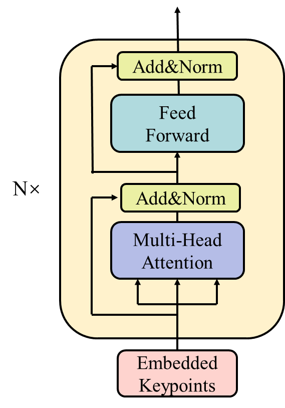
Figure 1: Structure of the transformer encoder

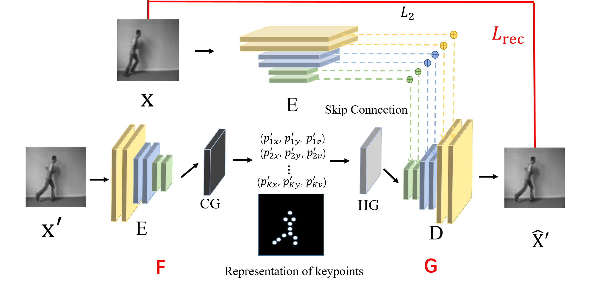
(a) Train the Keypoint Detector using $L_{rec}$ in Eq.(3).

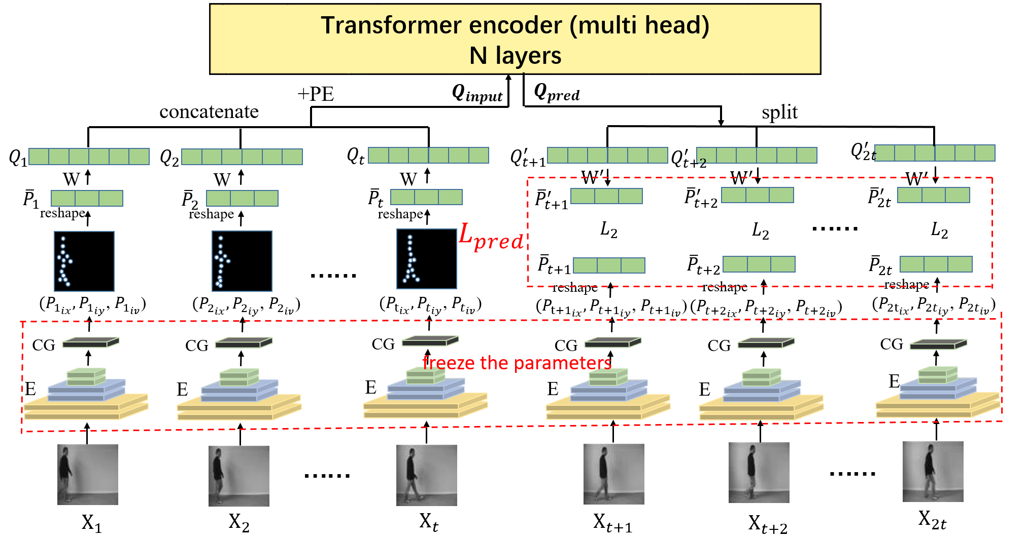
(b) Freeze the parameters of Keypoint Detector and train the Predictor using $L_{pred}$ in Eq.(14).

Figure 2: Two-step training

Figure 3: Detailed structure of TKN-Sequential

Transformer encoder. We use the transformer encoder structure from vaswani2017attention as shown in Figure 1. The transformer encoder uses a self-attention mechanism that calculates the relationship between the current and other inputs. In this paper, we use the transformer encoder to calculate how the keypoints of the current frame are composed of the previous keypoints. Self-attention is a function that maps a query (Q) and a set of key-value (K,V) pairs to an output.

Each input corresponds to a vector query of length $d_{q}$, a vector key of length $d_{k}$, and a vector value of length $d_{v}$. Suppose we have $l$ inputs denoted as $I\in\mathbb{R}^{l\times d_{model}}$, each of which has a dimension of $d_{model}$ as mentioned in the paper, there are $l$ query, key, and value vectors dentoed as $Q\in\mathbb{R}^{l\times d_{k}}$, $K\in\mathbb{R}^{l\times d_{k}}$, and $V\in\mathbb{R}^{l\times d_{v}}$, respectively. We use the fully connected layer to convert the inputs to Q, K and V:

$$\left\{\begin{array}[]{rcl}Q=IW^{Q}\\ K=IW^{K}\\ V=IW^{V},\end{array}\right.$$ (8)

where $W^{Q}\in\mathbb{R}^{d_{model}\times d_{k}}$, $W^{K}\in\mathbb{R}^{d_{model}\times d_{k}}$, and $W^{V}\in\mathbb{R}^{d_{model}\times d_{v}}$ are the conversion matrices. The self-attention of these matrices can be expressed as follows:

$$Attention(Q,K,V)=softmax(\frac{QK^{T}}{\sqrt{d_{k}}})V,$$ (9)

where $\sqrt{d_{k}}$ is used to prevent the gradient disappearance when the Q and K dot product is too big. In fact, we use multi-head self-attention mechanisms for better performance with more parameters. Each head refers a self-attention in Eq. (9). We concatenate all the heads together and pass them through a fully connected layer to get the result of the same dimension with the input $I$,

$$Multihead(Q,K,V)=concat(head_{1},...,head_{n})W^{h},$$ (10)

where $head_{i}=Attention(IW^{Q}_{i},IW^{K}_{i},IW^{K}_{i}),i=1,2,...,n$, $W^{h}\in\mathbb{R}^{nd_{k}\times d_{model}}$. We add the result to the input $I$ by residual connection and then normalize them by LayerNorm to solve the gradient disappearance:

$$x=LayerNorm(I+Multihead(Q,K,V)).$$ (11)

Considering that the self-attention mechanism may not fit complex processes well, the model is enhanced by adding two fully connected layers with a ReLU activation in between called Feed-Forward Network:

$$FFN(x)=max(0,xW_{1}+b_{1})W_{2}+b_{2},$$ (12)

Then we use Eq. (11) again to get the final result. We can either output the result directly or send it as input to the Transformer encoder for multiple iterations.

Two-step training. As shown in Figure 2, we used a two-step training: first we trained the Keypoint Detector using $L_{rec}$ in Eq.$(3)$ in the paper and then froze its parameters, then we trained the Predictor using $L_{pred}$ in Eq.$(14)$ in the paper.

Prediction Processes. Figure 3 shows the detailed structure of TKN-Sequential, in which $X^{{}^{\prime}}_{t+1}$ is the combination of predicted $\bar{P}^{{}^{\prime}}_{t+1}$ and the background information of $X_{t}$ extracted by the decoder. Note that “$\bar{P}^{{}^{\prime\prime}}_{t+1}$ and the background information of $X^{{}^{\prime}}_{t+1}$” are not equal to “$\bar{P}^{{}^{\prime}}_{t+1}$ and the background information of $X_{t}$”, albeit they are both extracted by the encoder from the $X^{{}^{\prime}}_{t+1}$. It is because two consecutive frames are very similar but still have some minor differences in the keypoints and background information, as mentioned in Section Prediction Processes in the paper. Following these processes, TKN-Sequential can capture the background information more accurately than TKN in long-range predictions when the background changes a lot.

Experimental setup

	boxing	handclapping	handwaving
TKN	0.897	0.908	0.898
TKN-Sequential	0.878	0.874	0.857
	jogging	running	walking
TKN	0.762	0.759	0.786
TKN-Sequential	0.783	0.775	0.820

Table 1: SSIM performances on different KTH’s actions.

Dataset.

KTH dataset includes 6 types of movements (walking, jogging, running, boxing, hand waving, and hand clapping) performed by 25 people in 4 different scenarios, for a total of 2391 video samples. The database contains scale variations, clothing variations, and lighting variations. We use people 1–16 for training and 17-25 for testing. Each image is converted to the shape of $(64,64,3)$.

Human3.6 dataset contains 3.6 million 3D human poses performed by 11 professional actors in 17 scenarios (discussion, smoking, taking photos and so on). We use scenario 1, 5, 6, 7, and 8 for training and 9 and 11 for testing. Each image is converted to the shape of $(128,128,3)$.

Following the manner of most baselines guen2020disentangling; wang2017predrnn; wang2018eidetic, we test long-range prediction performance on KTH and short-range prediction performance on Human3.6.

Baselines.

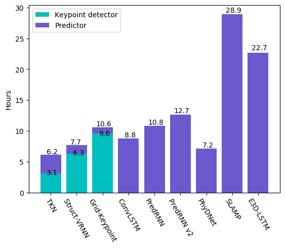
Figure 4: Total training time.

Method	SSIM$\uparrow$	PSNR $\uparrow$	TIME (ms)$\downarrow$	FPS$\uparrow$	Memory (MB)$\downarrow$	TIMES (ms)
			all model(test)	(test)	(test)	Predictor(test)
TKN (employs only the encoder)	0.865	27.49	86	233	1,447	7.2
TKN (employs whole transformer)	0.800	25.87	153	131	1,450	74

Table 2: Performance comparison of TKN’s prediction module between using only the transformer encoder and whole transformer.

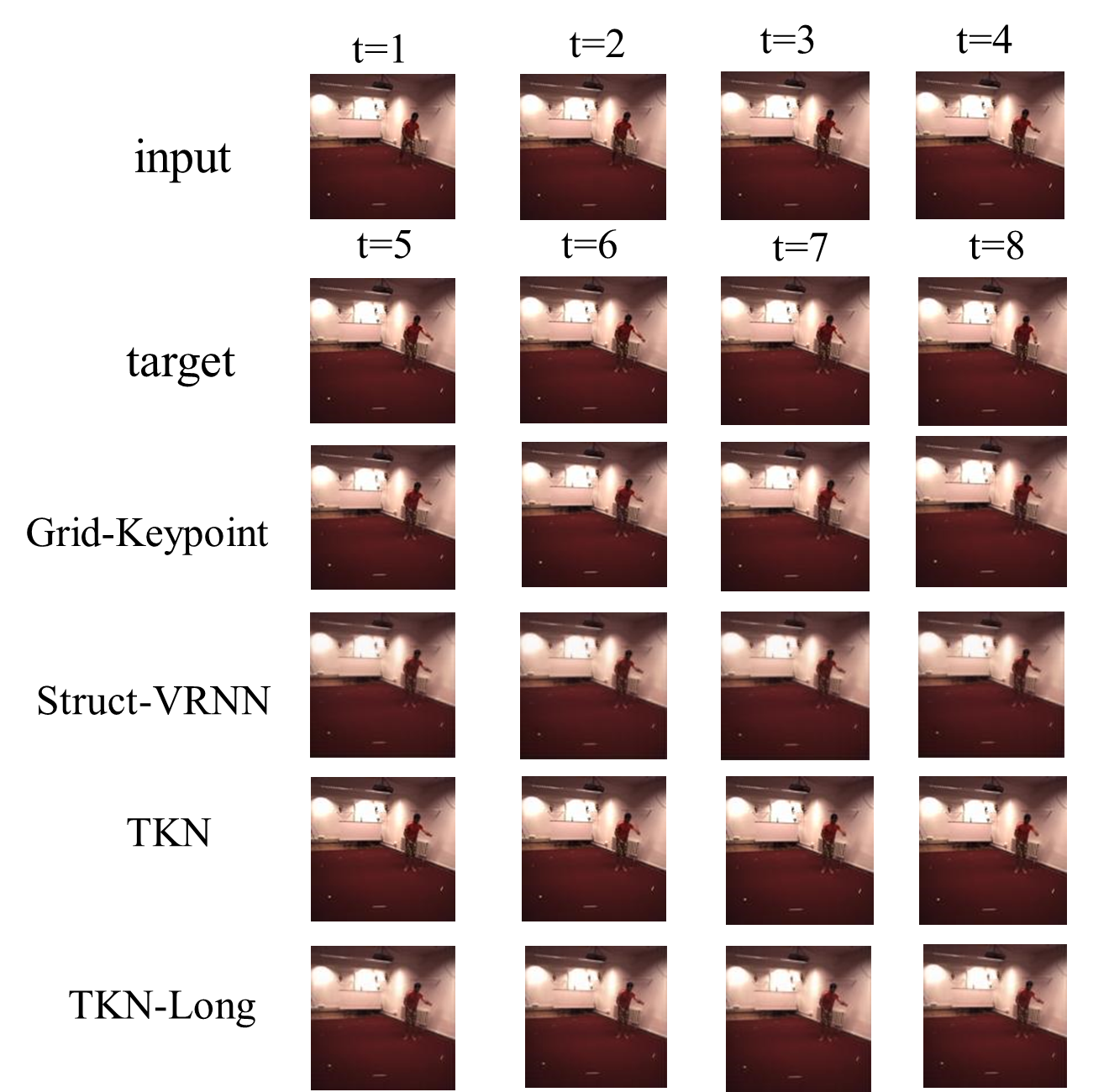
(a) Human3.6(1)

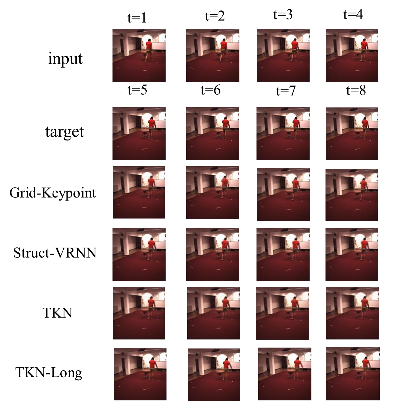
(b) Human3.6(2)

Figure 5: Results of short-range predictions on Human3.6.

To validate the performance of TKN, we select 8 most classical and effective SOTA methods as the baselines. For fair comparison, all these baselines are tested on Pytorch. The 8 baselines include: ConvLSTMshi2015convolutional, Struct-VRNNminderer2019unsupervised, Grid-Keypoint gao2021accurate, Predrnnwang2017predrnn, Predennv2wang2021predrnn, PhyDNetguen2020disentangling, E3D-LSTMwang2018eidetic, SLAMPakan2021slamp.

1. ConvLSTMshi2015convolutional is one of the oldest and most classic video prediction method based on LSTM.

2. Struct-VRNNminderer2019unsupervised is the first one to use keypoints to make prediction.

3. Grid-Keypointgao2021accurate is a grid-based keypoint video prediction method.

4. Predrnnwang2017predrnn is a classic prediction method adapted from LSTM.

5. Predennv2wang2021predrnn can be generalized to most predictive learning scenarios by improving PredRNN with a new curriculum learning strategy.

6. PhyDNetguen2020disentangling disentangles the dynamic objects and the static background in the video frames.

7. E3D-LSTMwang2018eidetic combines 3DCNN and LSTM to improve prediction performance.

8. SLAMPakan2021slamp is an advanced stochastic video prediction method.

Due to the lack or incompleteness of open-sourced code, we tested Predennv2 and SLAMP only on KTH dataset while the others on both datasets.

Model structures. TKN and TKN-Sequential have the same keypoint detector structure, which has a 6-layer encoder and a 6-layer decoder. Each encoder layer includes Conv2D, GroupNorm, and LeakyRelu. Each decoder layer includes TransposedConv2D, GroupNorm and LeakyRelu. Since the skip connection is used between encoder and decoder, the input dimension of each decoder layer is twice the output dimension of the corresponding encoder layer.

For the predictor, TKN uses a 6-layer transformer encoder with the input sequence length of 10, and TKN-Sequential uses 10 single-layer transformer encoders, each with an input sequence length of 10, 11, …, 19. As mentioned in Section Prediction Processes, each transformer encoder’s output of TKN-Sequential is averaged according to the input length, hence the output of both TKN and TKN-Sequential has a length of 10. All transformer encoders employed by the baselines share the same parameters: $d_{k}=d_{v}=64,d_{model}=512,d_{inner}=2048,n_{head}=8,dropout=0$

Results

KTH

We compare the performance of our models on the different action classes contained in KTH, each class with 100 randomly selected video sequences of each KTH’s action class for tests. As summarized in Table 1, TKN-Sequential performs better than TKN on actions with large movements such as walking, jogging, and running, while TKN performs better on handwaving, handclapping, and boxing which have smaller movements.

Overall training time. We compare the overall training time consumption considering various numbers of required epochs before convergence. Note that here TKN, Grid-Keypoint, and Struct-VRNN use the two-step training as mentioned in Section Experimental Setup of the paper. Although TKN’s predictor trains slower than Grid-Keypoint and Struct-VRNN because its Transformer encoder takes 750 epochs to reach the optima while Convlstm and VRNN takes only 20 and 50, TKN’s overall training speed is up to 2 to 3 times faster than the baselines as shown in Figure 4.

Human3.6

Figure 5(a) and 5(b) depict the comparison of TKN and baselines on the Human3.6 dataset for short-range prediction, as most baselines do. The changes of the actions may not be considerable due to the short period. But upon closer observation, we can tell that the lighting of the background and the movement of the person in TKN are closest to the goundtruth.

Ablation Experiments

Predictor. Table 2 compares the results of Predictor in TKN using the full transformer structure and only its encoder part. We can see that the encoder-only method works much better in terms of both prediction speed and accuracy. This is because the transformer, which was initially proposed to solve NLP problems, requires embedding each word’s label ID to a vector. Its translation process is similar to RNN’s cycle principle which compares each high-dimensional output with the embedding vectors to get the word ID, and then sends the corresponding embedding vector as the input to the transformer to translate the next word. In short, their input and output are finite discrete quantities, while the keypoints in our prediction task are continuous quantities that can’t be labeled with finite IDs, hence excluding the possibility of mapping the high-dimensional output to IDs. Moreover, since each output in our task, which is the next input, is a floating point which can’t be acquired with 100% accuracy, the small errors in each transformer cycle are accumulated.

The long prediction time of TKN (employs whole transformer) is because the translation part of the transformer is a step-by-step process and each step goes through a complete transformer, while TKN (emplys only the encoder) is able to output all the results in one step.

We also provide a comparison video of TKN and baselines in the attached file. The first second shows the observed content, and the later seconds show the predicted content. It can be seen that TKN and TKN-Sequential have clearer and more accurate video content than baselines. And TKN-Sequential is more accurate in details and shows more precise position predictions than TKN.