Aemulus ν

Aemulus $\nu$: Precise Predictions for Matter and Biased Tracer Power Spectra in the Presence of Neutrinos

Abstract

We present the Aemulus $\nu$ simulations: a suite of 150 $(1.05h^{-1}\rm Gpc)^{3}$ $N$-body simulations with a mass resolution of $3.51\times 10^{10}\frac{\Omega_{cb}}{0.3}~{}h^{-1}M_{\odot}$ in a $w\nu$CDM cosmological parameter space. The simulations have been explicitly designed to span a broad range in $\sigma_{8}$ to facilitate investigations of tension between large scale structure and cosmic microwave background cosmological probes. Neutrinos are treated as a second particle species to ensure accuracy to $0.5\,\rm eV$, the maximum neutrino mass that we have simulated. By employing Zel’dovich control variates, we increase the effective volume of our simulations by factors of $10-10^{5}$ depending on the statistic in question. As a first application of these simulations, we build new hybrid effective field theory and matter power spectrum surrogate models, demonstrating that they achieve $\leq 1\%$ accuracy for $k\leq 1\,h{\rm Mpc}^{-1}$ and $0\leq z\leq 3$, and $\leq 2\%$ accuracy for $k\leq 4\,h{\rm Mpc}^{-1}$ for the matter power spectrum. We publicly release the trained surrogate models, and estimates of the surrogate model errors in the hope that they will be broadly applicable to a range of cosmological analyses for many years to come.

1 Introduction

After recombination and on sufficiently large scales, the dynamics of the Universe can be described by the collisionless Boltzmann equation in an expanding background. Much of the theoretical effort in cosmology over the last few decades has been devoted to increasing the accuracy, flexibility, and speed of methods for solving these equations, with techniques generally falling into two camps: perturbation theory and simulation-based methods. In this work, we combine aspects of both of these methodologies in order to make accurate non-linear predictions for real-space power spectra in cold dark matter (CDM) cosmologies, including the effects of massive neutrinos and non-cosmological constant dark energy (DE) equations of state.

Perturbative methods for predicting matter density and velocity statistics have matured over the past few decades to the point that they are now commonly used to confront contemporary observations [1, 2, 3, 4, 5, 6]. Methods for incorporating the effects of dark energy [7], and massive neutrinos have been developed [8, 9, 10], although near $\Lambda$CDM cosmologies the Einstein de-Sitter approximation is typically accurate enough for current levels of observational errors [11]. While fast, flexible, and accurate over the range of scales where perturbation is valid, these methods inevitably break down in the non-linear regime of structure formation. With the incorporation of effective field theory (EFT) techniques, the reach of perturbation theory has been pushed to $k\sim 0.3\,h{\rm Mpc}^{-1}$ for real-space power spectra [12] and $k\sim 0.2\,h{\rm Mpc}^{-1}$ for redshift-space power spectra [13].

Methodologies for running $N$-body simulations more rapidly and in larger volumes have also seen a great deal of development in the last few decades [14, 15, 16, 17]. These simulations use a variety of methods to solve a discretized version of the non-relativistic, collisionless Boltzmann equation. They produce fully non-linear solutions, but great care must be taken to ensure that they are converged with respect to various choices that are made when running them, such as mass and time resolution, volume, and initial conditions.

A variety of methods for including the effects of massive neutrinos in $N$-body simulations have been developed. For sufficiently small neutrino masses, e.g. $\sim 0.3\,\textrm{eV}$ and below, treating the neutrino component linearly while solving for the full non-linear evolution of the CDM distribution is sufficient [18, 19, 20, 21, 22]. At larger masses, a non-linear treatment of the neutrino component is necessary to achieve sub-percent accuracy above $k\sim 1\,h{\rm Mpc}^{-1}$ [23, 24, 25, 22, 26]. Including neutrinos as a separate particle species in $N$-body simulations has been shown to be an accurate route for such a treatment [27, 28]. While the most widely used implementation of this method incurs significant biases in the neutrino distribution itself due to the impact of shot noise at early times when the neutrino auto-power spectrum is small, this complication is insignificant, as all currently relevant observables either depend on the total matter field, or the CDM and baryon fields, which are accurately recovered, albeit with slightly increased noise, using such a technique for realistic neutrino masses.

Although $N$-body simulations are able to accurately solve for non-linear CDM and neutrino dynamics, they are fundamentally limited in the scales that they can describe, as neglected processes such as radiative cooling, star formation and subsequent supernovae, as well as Mpc-scale outflows from supermassive black holes become non-negligible on the scales of galaxies and galaxy clusters. Furthermore, because $N$-body simulations do not include the actual objects that are observed in contemporary surveys, i.e. galaxies and other luminous tracers of the matter distribution, there will always be uncertainty associated with the connection between $N$-body simulations and galaxy surveys that must be appropriately accounted for in order to use these simulations to confront observations.

Traditional methods for connecting $N$-body simulations to galaxy survey observations involve statistical models for populating galaxies in simulated dark matter halos. Most common among these techniques is the halo occupation distribution (HOD) formalism [29, 30, 31], which assumes functional forms for the distribution of the number of galaxies that occupy halos of a given mass, as well as the phase-space distribution of those galaxies within a halo. The end product of this technique is a catalog of simulated galaxies, from which various summary statistics can be computed and compared to observational data. $N$-body simulations paired with the HOD formalism have recently been used to extract cosmological constraints from a range of data sets, including redshift-space clustering [32, 33, 34, 35], galaxy–galaxy lensing [36, 37], and higher-order statistics of the galaxy field [38, 39].

There are two major limitations of the HOD formalism, which also apply to many other methods for statistically populating simulated dark matter halos with galaxies. The first is that such methods are significantly restricted by their reliance on halo-finding algorithms. In order to model galaxy samples that populate low mass halos, the simulations must resolve these halos, placing stringent requirements on the resolution of the simulations and thus increasing the expense of running these simulations. Historically, this restriction has been one of the main inhibitors in using simulations to analyze large scale structure data. Relatedly, the halo definition employed in data analysis matters (e.g. [40]). Different choices of halo definition can lead to very different resolution requirements [41, 42], and different conclusions about the necessity of parameters beyond halo mass in the HOD parameterization [43, 44].

The second limitation is more philosophical, namely that the functional form parameterizations used in HOD models draw motivation from hydrodynamical simulations. These simulations are able to model the formation of galaxies, and thus directly measure the relevant quantities required for HOD models. Although such simulations have made significant progress in terms of reproducing observations over the last decade [45, 46, 47, 48], they still rely heavily on sub-grid physics models with tens of parameters that are hand tuned to match observations. Thus the extent to which these simulations are predictive is limited, and the accuracy of their predictions seldom meets the stringent requirements of cosmological parameter estimation. Furthermore, because hydrodynamical simulations are relied on to help determine key ingredients of HOD models, there is no controlled series of HOD terms that one can systematically check sensitivity to when performing data analysis. Nevertheless, if these uncertainties can be satisfactorily controlled, then HOD and related methods paired with high resolution $N$-body simulations have the potential to extract information from significantly smaller scales than perturbation theory.

On the other hand, the bias expansions used to connect matter statistics to observed tracer statistics in perturbation theory are well controlled: at a given order there are a finite number of terms that obey the symmetries of the problem in question, and analyses can be systematically checked for sensitivity to these terms. Furthermore, these expansions are flexible enough to model any biased tracer. Because of these advantages, significant effort has been invested in the last few years in using the principles of perturbative bias expansions to connect $N$-body simulations to observables, a methodology that has become known as hybrid effective field theory (HEFT). HEFT was first introduced in [49], where it was demonstrated that appropriately post-processed outputs of $N$-body simulations can replace the perturbation theory basis spectra that are used in the bias expansion. This work showed that such a technique enables one to fit real-space halo power spectra to $k=0.6\,h{\rm Mpc}^{-1}$, a factor of three smaller in scale than what is possible with Lagrangian perturbation theory (LPT). [50] demonstrated that HEFT could also accurately model summary statistics sensitive to higher-order auto- and cross-clustering of tracers and matter [51, 52] on quasi-linear scales ($\gtrsim 15h^{-1}{\rm Mpc}$).

One sacrifice that must be made when exchanging perturbatively predicted basis spectra for their analogous simulation-based predictions is that the cosmology dependence of these spectra must then be predicted by running simulations at many different cosmologies. Running a new simulation for each cosmology sampled in a Monte Carlo Markov Chain (MCMC) analysis would be a prohibitively expensive endeavor, but significant progress has been made in the last decade on so-called “emulation” or “surrogate modeling” techniques that circumvent the need for this. These techniques interpolate between measurements made from small suites of simulations run at a few different cosmologies in order to obtain accurate predictions over the entire range of cosmologies spanned by the simulations. Constructing such surrogate models has become relatively commonplace, with simulation-based models now existing for the matter power spectrum [53, 54, 55], the halo mass function [56, 57], linear halo bias [58, 59], galaxy clustering and lensing statistics [60, 61, 62, 33], higher-order statistics [38, 39], as well as HEFT models for a number of statistics [63, 64, 65, 66, 67].

Another sacrifice that must be made when using simulation-based predictions is that sample variance is introduced due to the finite volumes that simulations are run in. A number of methods have been introduced to mitigate the effect of sample variance on simulated measurements. The most commonly used method is called fixed amplitude simulations, where instead of initializing the amplitude of each Fourier mode of the simulation with a Rayleigh distributed random number, the amplitude of each mode is fixed to its expectation value [68, 69]. In combination with this, a second simulation is often run where each Fourier mode is taken to be $180^{\circ}$ out of phase with the first simulation [70, 69]. Together these methods are called “paired and fixed” simulations, and have been used to reduce the variance of measurements from a number of suites of simulations [71, 54, 72]. These methods come with a cost though, as they require one to run twice as many simulations. They also forego Gaussian initial conditions and thus statistics measured from them must be painstakingly examined for biases [73, 74, 75]. Finally, the improvements in variance obtained from paired-and-fixed simulations degrade significantly with non-linear and higher-order statistics [74, 75].

The method of control variates [76] offers an alternative to paired and fixed simulations that does not suffer from these drawbacks. Control variates allow for the reduction in variance of a random variable in the presence of a correlated random variable with known mean. This technique was introduced to the cosmology literature under the name ‘Convergence Acceleration by Regression and Pooling’ (CARPool) [77, 78, 79] in order to reduce the variance of measurements made from $N$-body simulations, where the control variate was taken to be measurements from approximate simulations such as COLA [80] or FASTPM [81]. [82] and [83] demonstrated that comparable variance reduction is possible at significantly less expense by using the Zel’dovich approximation (ZA) as the control variate to reduce the variance of real and redshift-space power spectra measured from $N$-body simulations, respectively.

In this work, we present a new suite of 150 simulations, run in a $w\nu$CDM cosmological parameter space, simulating neutrinos as an extra particle species to ensure accuracy of our predictions to $0.5\,\textrm{eV}$. Furthermore, we run these simulations in the broadest parameter space ever used in a single suite of simulations in order to ensure that they are accurate over the full range of $w\nu$CDM cosmologies allowed by current data. We perform convergence tests of these simulations to ensure their accuracy and we take advantage of the Zel’dovich control variate (ZCV) method to reduce the variance of the HEFT spectra that we measure from our simulations. We then build a surrogate model for these HEFT spectra, including the matter power spectrum.

This rest of this work is organized as follows. In Section 2, we describe the parameter space that the simulations are run in, focusing on how we optimized it to deliver both breadth and accurate surrogate models. In Section 3 we describe the settings used for our $N$-body simulations, emphasizing the improved accuracy provided by initializing our simulations at relatively low redshift using 3rd-order LPT. Section 4 introduces the basics behind LPT and HEFT and Section 5 describes our ZCV methodology and resultant improvements in the precision of our HEFT measurements. Section 6 describes our surrogate modeling methodology, quantifies the accuracy of the final HEFT models, and provides comparisons to previous matter power spectrum surrogate models. Finally, in Section 7 we summarize our results, detail our data release plans, and discuss future directions of inquiry.

2 Parameter Space Design

The design of surrogate model parameter space is crucial for ensuring reliable analysis results, and it requires balancing two factors: parameter space breadth and surrogate model accuracy. Covering a broad parameter space is complicated by “tensions” that have arisen in contemporary cosmological constraints [84, 85, 86, 87]. To avoid being biased by these tensions, simulations must span the range of parameter values that both sets of experiments prefer. To achieve this goal, the simulations’ parameter space should be as broad as possible without exceeding a fixed threshold for model accuracy. We set a goal of $1\%$ accuracy for two main reasons. First, $N$-body codes agree to $\sim 0.5\%$ at $k\sim 1\,h{\rm Mpc}^{-1}$ for the $z=0$ matter power spectrum [14], and so this sets a hard lower limit on how accurate a simulation based matter power spectrum model can be. Secondly, ongoing and upcoming surveys such as the Dark Energy Spectroscopic Instrument [88], Rubin Observatory [89], Simons Observatory [90] will measure angular weak lensing and galaxy clustering spectra at roughly $1\%$ precision, as demonstrated in Figure 1. We have made the forecasts in this figure assuming a disconnected covariance approximation, which should place a lower bound on the actual errors on these spectra. For DESI we have assumed $\bar{n}=6\times 10^{-4}\,h^{3}\rm{Mpc}^{-3}$ and biases as measured in [91], consistent with the DESI luminous red galaxy number density at $z\sim 0.7$ [92], in a bin of roughly constant density between $z=[0.6,0.8]$. For Rubin, we take $\sigma_{e}=0.26$ and use a number density that is consistent with a quarter of the LSST gold sample [93], $\bar{n}=10.8\,{\rm arcmin}^{-2}$, and a source distribution that matches the gold sample at $z\geq 1$ convolved with photometric redshift uncertainties. SO noise curves are taken from [94], and for all three surveys we assume $f_{\rm sky}=0.4$. The angular band powers shown have a width of roughly $\Delta\ell\sim 3\sqrt{\ell}$. We have also plotted the error on the galaxy angular auto-power spectrum that the model in this work achieves, computed as described in Section 6.3 to illustrate that the final accuracy of our model is sufficient for upcoming data, although see discussion in that section related to error correlations between different scales. This is an conservative bound compared to the emulator error achieved on the galaxy–matter angular power spectrum or the matter-matter power spectrum for these redshift bins.

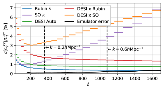
Figure 1: Forecasted fractional uncertainties on angular galaxy and CMB lensing, and galaxy clustering auto- and cross-power spectra from ongoing and upcoming surveys. The assumptions we have made in computing these are described in the main text. The dashed vertical lines represent the approximate angular scales that correspond to $k=0.2\,h{\rm Mpc}^{-1}$, the $k_{\rm max}$ assumed in most analyses that use pure perturbation theory models, and $k=0.6\,h{\rm Mpc}^{-1}$, the approximate $k_{\rm max}$ to which HEFT is unbiased [63], for an effective redshift of $z=0.7$ where the DESI sample is assumed to be centered. We also plot our measured emulator error for the DESI auto spectrum at this redshift, computed as described in Section 6.3, to illustrate that the accuracy we achieve in this work is significantly below the statistical errors of the measurements considered here.

Additionally, it is important to have confidence that the chosen parameter space sampling will deliver the desired level of accuracy before running any simulations. To address this concern, we produce mock matter power spectrum measurements using HMcode2020 [95], assuming a fixed number of simulations, while varying the bounds of the parameter space. We then build surrogate models for these spectra and test their accuracy against a dense sampling of HMcode2020 predictions that were not included in the surrogate model training.

Here we aim to span a range of parameters in the $w\nu$CDM cosmological model, including the matter density $\omega_{m}$, the baryon density $\omega_{b}$, the dark energy equation of state parameter $w$, the Hubble parameter $H_{0}$, the scalar spectral index $n_{s}$, the normalization of the power spectrum $A_{s}$, and the sum of neutrino masses $\sum m_{\nu}$. The parameters $\omega_{b}$ and $n_{s}$ are tightly constrained by CMB data, and their impact on LSS observables is minor [88, 54, 58]. We set their bounds to $0.0173\leq\omega_{b}\leq 0.0272$, and $0.93\leq n_{s}\leq 1.01$, broader than is allowed by current CMB constraints; the small impact these parameters have on LSS observables means that our surrogate model errors are not significantly affected by this breadth. We set broader limits on the other parameters, as they have a more significant impact on LSS observables. We use a prior on the logarithm of the sum of the neutrino masses $\sum m_{\nu}$, using a range that is constrained by combinations of CMB and LSS data [88, 96] and by laboratory-based experiments [97]: $0.01,\textrm{eV}\leq\sum m_{\nu}\leq 0.5,\textrm{eV}$. The lower edge of the range is set below the current minimum allowed value of $0.06\rm eV$ [98, 99] to avoid modeling errors at the minimum allowed mass.

We also investigate the impact of varying the widths of our parameter space in $\log 10^{10}A_{s}$, $w$, $\omega_{c}$ and $H_{0}$ on the accuracy of the resulting surrogate models. In particular, we generate experimental designs in a four-dimensional grid, such that the bounds of each design are

$$10^{9}A_{s} \in[2.1-0.33i,2.1+0.33i]$$

$$w \in[-1-0.28j,-1+0.28j]$$

$$\omega_{c} \in[0.12-0.02k,0.12+0.02k]$$

$$H_{0} \in[67-7.5l,67+7.5l]\,,$$

and $i,j,k,l\in\{1,2,3\}$.

We sample each of this set of 81 parameter bounds with 100 points in a Latin hypercube, maximizing the minimum distance between pairs of points in two dimensions. At each point in parameter space, we produce non-linear matter power spectrum predictions using HMCode2020 [95], $P_{m,m}^{\rm HM}(k,z)$, and 1-loop LPT predictions of the matter power spectrum $P_{m,m}^{\rm 1\textrm{-}loop}(k,z)$, as will be described in more detail in Section 4. We evaluate these models at 100 points, logarithmically spaced between $k=10^{-1}\,\,h{\rm Mpc}^{-1}$ and $k=1\,\,h{\rm Mpc}^{-1}$, at the same redshifts that we output snapshots at, described in Section 3.

We build surrogate models for the logarithm of the ratio of these predictions:

$$\Gamma=\log_{10}(P_{m,m}^{\rm HM}(k,z)/P_{m,m}^{\rm 1\textrm{-}loop}(k,z))\,,$$ (2.1)

reproducing the surrogate modeling methodology in [63] using a combination of principal component analysis (PCA) and polynomial chaos expansions (PCE). We performed a hyper-parameter optimization, using the same methodology as described in Section 6, on the design with ${i,j,k,l}=2$. We have tested sensitivity to which design this optimization is performed on and found negligible impact to our conclusions. One notable difference to the procedure described in Section 6, is that here we have used redshift as our time variable, rather than using $\sigma_{8}(z)$ as we do in Section 6. This is because before running our simulations, we did not consider this option and our design choices were made using redshift as a time variable, so we have not altered this after the fact.

In order to test the surrogate models trained on these 81 parameter spaces, we produce a test set of 10,000 models over the broadest parameter space considered here, i.e. ${i,j,k,l}=3$. When measuring errors for each choice of parameter limits, we require that the test points lie within the hypercube defined by the minimum and maximum value of each parameter in the design under consideration, such that the number of test points varies from design to design.

In Figure 2, we show the 68th percentile error for a sub-selection of parameter space designs. It is clear that as we expand the boundaries of our parameter space, the surrogate model errors become larger. The main notable feature is that surrogate model performance is very sensitive to the chosen bounds on the dark energy equation of state parameter, $w$. Only designs with $j=1$ achieved our goal of sub-percent 68th percentile error over the entire range of scales considered. Given the current constraints on $w$ from individual LSS probes, we determined that this choice would be too restrictive.

Because of this, we chose employ a two-tiered parameter space design, with the first tier of 100 simulations, sampled using a Latin hypercube, spanning as broad a parameter space as possible while not exceeding $2\%$ 68th percentile error, and a more restricted second tier of 50 simulations, sampled with a Sobol sequence [100], where the 68th percentile error is less than $1\%$. We have used a Sobol sequence for this second tier so that it is straightforward to add additional simulations in the future by using the next element of the Sobol sequence. Figure 3 shows the parameter space sampling resulting from this optimization compared with that used in Aemulus $\alpha$ [101], as well as the cosmological constraints presented in [87]. Table 1 lists the boundaries for the Tier 1 and Tier 2 parameter spaces. Note that these are the bounds of the Latin hypercube and Sobol sequence respectively, and not the actual minimum and maximum values of simulated cosmologies, although the difference between these is negligible. In Section 6 and Appendix A we demonstrate that the accuracy that we achieve with our $N$-body based surrogate models is consistent with our forecast error, and explore the HMCode2020 surrogate model error as a function of cosmological parameters for the final design used for the Aemulus $\nu$ simulations.

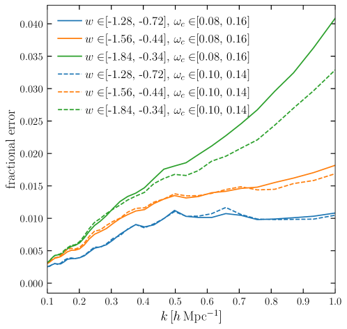
Figure 2: 68th percentile fractional error for HMCode2020 surrogate models as a function of $k$ for a sub-selection of the 81 parameter space bounds considered. The main feature of note is that the surrogate model error depends significantly on the range of dark energy equation of state parameters that we include in the training domain. Because of this, we have opted to use two tiers of simulations, in order to allow for broad exploration of DE parameter space, while still maintaining very high accuracy near $\Lambda$CDM .

	Tier 1 min.	Tier 1 max.	Tier 2 min.	Tier 2 max.
$10^{9}A_{s}$	1.10	3.10	1.77	2.43
$n_{s}$	0.93	1.01	0.93	1.01
$H_{0}$	52.0	82.0	59.5	74.5
$w$	-1.56	-0.44	-1.28	-0.72
$\omega_{b}$	0.0173	0.0272	0.0198	0.0248
$\omega_{c}$	0.08	0.16	0.11	0.13
$\sum m_{\nu}\,(\textrm{eV})$	0.01	0.50	0.01	0.50

Table 1: Aemulus $\nu$ parameter space boundaries.

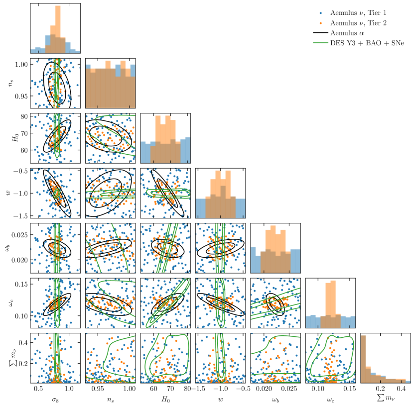
Figure 3: Comparison of the Aemulus $\nu$ parameter space sampling to that used in Aemulus $\alpha$. Blue and orange points represent our tier 1 and 2 simulations respectively, while black points are cosmologies used for the Aemulus $\alpha$ simulations. For reference, we also plot constraints from the combination of DES Y3 weak lensing and galaxy clustering combined with BAO and type Ia supernovae [87, 96] (green), as well as Planck 2018 constraints combined with the same BAO and type Ia supernovae data (red) [88, 96].

3 Initial Conditions and $N$-body solver

Appropriate initialization of simulations is as important for obtaining converged $N$-body predictions as any setting in the $N$-body solver itself. In particular, it has been shown that early initialization of simulations with low order LPT can lead to appreciable transient errors in force calculations [102, 103]. These transients are sourced by sparse sampling of modes around the Nyquist frequency, $k_{\rm nyq}$, of the initial particle grid, leading to an incorrect growing mode in the simulations until gravitational collapse leads to denser sampling on these scales [104]. The impact of this effect becomes more appreciable for higher-order statistics, where anisotropy in the particle distribution due to the imprint of the grid causes an even larger impact. [103] showed that this transient effect can be alleviated by starting simulations at significantly later cosmic times than previously used, enabled by using third-order LPT (3LPT) to initialize the particle distributions, as implemented in the monofonic code. [105] then extended monofonic to treat massive neutrinos by implementing an approximate three-fluid 3LPT. In this work, we make use of this extended version of monofonic to generate initial CDM and neutrino particle distributions at $z=12$ using 3LPT.

The presence of massive neutrinos imparts a scale-dependent growth, $D(k,z)$, to the matter distribution that disallows the typical practice of back-scaling a $z=0$ linear matter power spectrum using a scale-independent growth factor to initialize simulations. Instead, we compute the linear CDM and baryon ($cb$) power spectrum, $P_{cb,\rm{lin}}(k,z=0)$, using CLASS [106], and back-scale to our starting redshift $z_{\rm ini}$ using a scale dependent growth factor, $D_{cb}(k,z_{\rm ini})$, that is computed using a first-order Newtonian fluid approximation as implemented in zwindstroom [105]. Conveniently, this also accounts for the lack of a radiation component in our simulations, as well as the fact that Newtonian mechanics breaks down at the highest redshifts and very largest scales that we simulate [107].

The initial $cb$ power spectrum is then given by

$$P_{cb}(k,z_{\rm ini})=D_{cb}(k,z_{\rm ini})^{2}P_{cb,\rm{lin}}(k,z=0)\,.$$ (3.1)

This is the quantity that is used to generate our initial Gaussian density field, from which we compute displacements in order to initialize the $cb$ particle distribution with 3LPT as implemented by monofonic . This re-scaling only works exactly at linear order at $z=0$, but it has been shown to achieve $\sim 0.1\%$ accuracy at redshifts relevant for LSS studies [107]. As discussed above, using 3LPT allows us to initialize our simulations significantly later than would otherwise be possible with lower-order LPT models. We note that beyond-linear LPT treatment of neutrinos is not particularly important, as the neutrino overdensities remain small to very low redshifts due to the effect of free streaming. Using 3LPT for $\delta_{cb}$ is, however, essential in order to start at $z_{\rm ini}=12$ [103].

We generate neutrino particle initial conditions using fastDF[108], which produces initial particle displacements and velocities at $z=12$ by integrating neutrino particles along geodesics starting from $z=10^{9}$ using the linear metric perturbations output from CLASS. We set the fastDF time stepping parameter to $\Delta\log a=0.05$, with a mesh size of $M=384$, as these settings are shown to lead to converged results in [108]. We assume that all three neutrinos have equal masses, usually referred to as the degenerate mass approximation. This has been shown to be a good approximation to both inverted and normal hierarchy scenarios, and is significantly more accurate than assuming one massive and two massless neutrinos [27].

We make use of modified version of Gadget-3 in order to evolve our $cb$ and neutrino particle distributions from $z_{\rm ini}=12$ to $z=0$. We use $1400^{3}$ $cb$ and neutrino particles respectively with a box size of $L_{\rm box}=1050\,h^{-1}\rm Mpc$, yielding a $cb$ particle mass of $3.51\times 10^{10}\frac{\Omega_{cb}}{0.3}~{}h^{-1}M_{\odot}$. We use a Plummer-equivalent force softening of $\epsilon_{\rm plummer}=20\,h^{-1}\rm kpc$, a mesh size of $N=2100$ for large-scale force computations and a maximum time step of $\rm{max}[\Delta\ln a]=0.01$. In order to facilitate arbitrary background evolution models, we have modified Gadget-3 to read in a tabulated $H(z)$ as output by zwindstroom, which accounts for relativistic corrections to $H(z)$ and allows us to simulate non-cosmological constant dark energy models. We have also modified Gadget-3 to only compute forces from neutrinos at the particle mesh level. This is an extremely accurate approximation, as neutrinos do not cluster significantly on scales smaller than the mesh resolution $L_{\rm box}/N=0.5\,h^{-1}\,\rm Mpc$, as visually illustrated in 4. This allows us to run simulations with neutrino particles that take only approximately $10\%$ longer than the same simulation without neutrinos. These settings are summarized in Table 2.

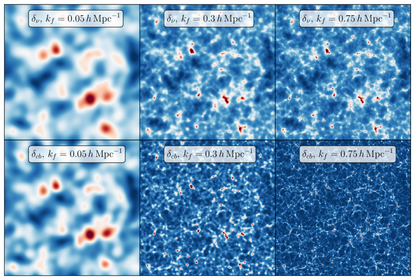
Figure 4: The top row shows the neutrino overdensity field, $\delta_{\nu}(z=0)$, smoothed with a Gaussian filter of width $k_{f}=0.05\,\,h{\rm Mpc}^{-1}$ (left), $k_{f}=0.3\,\,h{\rm Mpc}^{-1}$ (middle), and $k_{f}=0.75\,\,h{\rm Mpc}^{-1}$ (right) for the simulation in our suite with the largest neutrino mass. The bottom row shows the same but for the CDM field, i.e. $\delta_{cb}(z=0)$. For the largest smoothing scale, which is larger than the free streaming length of the neutrinos, the $cb$ and neutrino fields are almost identical. For progressively smaller smoothing scales, the $cb$ field continuously exhibits more structure, while the neutrino field remains very similar between the middle and right most columns. This visually illustrates that the neutrino component does not cluster on scales close to the grid scale.

$N_{\textrm{sim}}$	$L_{\text{box}}$ $[h^{-1}\textrm{Mpc}]$	$N_{cb}$	$N_{\nu}$	$m_{\text{part},cb}$ $[h^{-1}\textrm{M}_{\odot}]$	$\epsilon$ $[h^{-1}\textrm{kpc}]$	$\Delta\ln a_{\textrm{max}}$	$z_{ini}$
150	$1050$	$1400^{3}$	$1400^{3}$	$3.30\times 10^{10}\left(\frac{\Omega{cb}}{0.3}\right)$	20	0.01	12

Table 2: Summary of the settings used to run the Aemulus $\nu$ simulations. Columns are the total number of simulations, simulation side length, number of $cb$ and neutrino particles, $cb$ particle mass, Plummer equivalent force softening, maximum time step, and starting redshift.

We output fixed time snapshots at 30 epochs logarithmically spaced in scale factor between $z=3$ and $z=0$. Halo finding is performed on each snapshot with Rockstar, using strict spherical overdensity masses with $\Delta=200_{m}$, where strict refers to the inclusion of unbound particles in the mass estimates of halos. Halos finding is performed with only $cb$ particles. All results relating to halos in this work use only host halos, i.e. those halos that are not enclosed by halos with a higher maximum circular velocity.

3.1 Convergence tests

We made two changes to the accuracy settings of the Aemulus $\nu$ simulations compared to those used in [101]. First, we decreased the maximum allowed time step to $\rm{max}[\Delta\ln a]=0.01$ from $\rm{max}[\Delta\ln a]=0.025$. This change was made to ensure accurate recovery of linear growth on large scales, which was only achieved at $\sim 1\%$ accuracy in the Aemulus $\alpha$ simulations. We did not perform additional convergence tests of this change, because it is more conservative than our previous choice. However, we note that this change is one of the reasons that we are able to recover linear growth accurately, as discussed in Section 6.

Second, we lowered the starting redshift of our simulations from $z_{\rm ini}=49$ to $z_{\rm ini}=12$. While [103] tested the reliability of this choice, their simulations used slightly different settings, including a larger particle mass, than those used here. The accuracy of a particular starting time and LPT order depends on the resolution of the simulation: higher resolution simulations require earlier starting times at fixed LPT order because they resolve smaller scales that become non-linear earlier. Therefore, we need to make sure that the findings in [103] hold for the exact settings we used for Aemulus $\nu$ . We will now present a series of tests to show that starting at $z_{\rm ini}=12$ produces more converged results compared to starting our simulations at a higher redshift.

To perform our convergence tests, we have run three simulations, all at the Planck 2018 best fit $\Lambda$CDM cosmology [88]. The first simulation, which we call T0, uses identical settings to our fiducial simulations, but is run in a reduced volume of $(525\,h^{-1}\rm Mpc)^{3}$, evolving $700^{3}$ $cb$ particles and $700^{3}$ neutrino particles, using a particle mesh size of $1050^{3}$. The second simulation, which we call T1, is identical to T0, except we use $z_{\rm ini}=24$. The final simulation, T2, is identical to T1, but evolves $4\times 700^{3}$ $cb$ particles and $4\times 700^{3}$ neutrino particles, sampling the exact same modes as T0, using the “face-centered-cubic” lattice mode in monofonic . Because particle discreetness effects decrease with the number of particles used in the simulation, we can start the T2 simulation earlier and thus it provides a test of whether 3LPT is sufficiently accurate at $z=12$. We have run these simulations in a reduced volume because we only wish to compare relative differences between them, and so can use the same initial seed in order to remove sample variance from our comparisons.

Figures 5 and 6 show comparisons of these three test simulations, where all figures show fractional errors comparing T0 and T1 to T2. Figure 5 shows comparisons of real- and redshift-space $cb$ power spectra between the three simulations. The left hand panel depicts the fractional error on the real-space $cb$ power spectrum as a function of redshift. We see that starting at $z_{\rm ini}=24$ leads to significantly larger errors at fixed $k$ compared to $z_{\rm ini}=12$. This effect is amplified at high redshift, mostly due to the fact that the amplitude of the power spectrum is lower, so a similar absolute error translates into a larger fractional error. The redshift-space monopole, $P_{0,cb}$ does not exhibit the same trends, likely because the finger-of-god effect has washed out these subtle issues on small scales. The redshift-space quadrupole, $P_{2,cb}$, is recovered slightly better in T0 than T1, but the effect is again difficult to interpret due to the large role that virial velocities play at high-$k$ in redshift-space statistics. Nevertheless, we see that our fiducial settings are converged at the $\leq 1\%$ level to $k\sim 1\,h{\rm Mpc}^{-1}$ compared to the higher resolution T2 simulation.

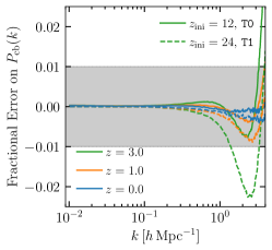
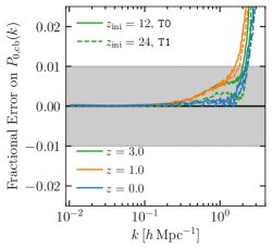
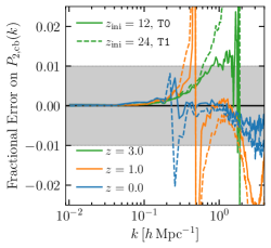
Figure 5: Comparison of real-space power spectra (left), monopole (middle) and quadrupole (right) of redshift space $cb$ power spectra between the T0 simulation started at $z=12$ (solid) and the T1 simulation started at $z=24$ (dashed) to the T2 simulation initialized at $z=24$ with four times the number of particles, but sampling the exact same modes. Initialization at $z=12$ with 3LPT yields the best results compared to this higher resolution simulation.

Figure 6 shows similar comparisons to Figure 5, but focuses on halo statistics. The left side shows fractional errors on the spherical overdensity halo mass function for the T0 and T1 simulations, again compared to the higher resolution T2. Error bars are estimated via jackknife resampling, using 128 jackknife regions. We see that for $z=1$ and $z=0$ both simulations are converged to at the $\leq 1\%$ level until $\sim 10^{13}\,h^{-1}M_{\odot}$, after which the T1 simulation begins to diverge. The T0 simulation remains converged at the $\leq 1\%$ until $\sim 2\times 10^{12}\,h^{-1}M_{\odot}$. Compared to our findings in the Aemulus $\alpha$ suite of simulations, starting our simulations at $z_{\rm ini}=12$ yields halo masses that are converged at a factor of two lower in mass, with the same mass resolution and force softening. At $z=2$, both T0 and T1 are converged at the $\sim 2\%$ level until $\sim 4\times 10^{12}\,h^{-1}M_{\odot}$. At $z=3$ both the T0 and T1 simulations diverge significantly from the T2 simulation at all masses measureable in these simulations and so we do not plot statistics for this redshift.

The right hand side of Figure 6 shows halo redshift-space monopole measurements for the same redshift outputs, where we use halos in a bin of mass from $12.5\leq\mathrm{lg}M\leq 13$. We observe a similar trend in convergence as for the mass function, where for $z<2$ both simulations are converged with respect to the higher resolution simulation. At high $k$, the T1 simulation deviates by $\sim 2\%$, although when we select samples by cumulative abundance rather than mass this discrepancy disappears, suggesting that it is simply a difference in shot noise due to the slightly different number densities of the mass selected samples in this simulation. The $z=3$ outputs from T0 and T1 exhibit a significant deviation from T2 and so we do not plot them. Higher multipoles are too noisy to be of use in these comparisons. In general this shows that masses and two-point clustering statistics of halos with $\lg M>12.5$ and $z<2$ are converged at the $\sim 1-2\%$ level, and halos from the $z=3$ outputs should not be used in these simulations.

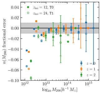
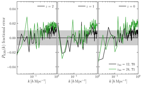
Figure 6: (Left) Same as Figure 5, but comparing halo mass functions. Again we see that the T0 simulation started at $z=12$ slightly outperforms the T1 $z=24$ simulation in comparison to the higher resolution T2 reference simulation started at $z=24$. The only exception to this is for $z=2$ where T0 and T1 perform comparably. At $z=3$ the mass functions are not converged at the $>5\%$ level for any masses measureable in these simulations, and so we do not plot them and caution against the use of the $z=3$ outputs from these simulations in general. At the two lower redshifts shown, the error on the halo mass function in the $z_{\rm ini}=12$ simulation remains below $1\%$ until $\sim 2\times 10^{12}h^{-1}\,M_{\odot}$, whereas the later start deviates by more than a percent by $\sim 5\times 10^{12}h^{-1}\,M_{\odot}$. (Right) Same as Figure 5, but comparing the monopole of the halo redshift-space power spectrum, measured in a halo mass bin of $10^{12.5}h^{-1}\,M_{\odot}\leq M_{200\rm b}<10^{13}h^{-1}\,M_{\odot}$. Again we see that at $z\leq 2$ the agreement between the T0 and T2 simulations is at the $\leq 1\%$ level. The T1 simulation and T2 agree until $k\sim 0.5\,h{\rm Mpc}^{-1}$, after which they begin to disagree by more than one percent. A similar trend is seen for the real-space halo power spectrum as well, although we do not display it here. At $z=3$, the halo (real and redshift space) power spectra for both T0 and T1 simulations disagree with the T2 by $\sim 2\%$ at all $k$.

4 Lagrangian perturbation theory and hybrid effective field theory

The utility of LPT extends beyond the simple use case of initializing $N$-body simulations. In particular, it has proven to be a highly effective model for the density fields of biased tracers in CDM cosmologies [109, 3]. In this work, we make use of LPT in two ways. First, we use the ZA as a control variate to reduce the cosmic variance of our simulated measurements. We also construct a surrogate model for HEFT measurements from our simulations, which can be seen as a non-perturbative extension of LPT. In this section, we introduce some basic LPT notation to clarify our presentation of these two aspects later in this work.

In LPT, we can express the combined CDM and baryon density field as

$$1+\delta_{cb}(\mathbf{x},a)=\int d^{3}\mathbf{q}\,\delta^{D}(\mathbf{x}-\mathbf{q}-\Psi(\mathbf{q},a))\,,$$ (4.1)

where

$$\mathbf{x}=\mathbf{q}+\Psi(\mathbf{q},a)\,,$$ (4.2)

and $\Psi(\mathbf{q},a)$ is computed perturbatively, such that

$$\Psi(\mathbf{q},a)=\sum_{n=1}^{\infty}\Psi^{(n)}(\mathbf{q},a).$$ (4.3)

Truncating this sum at $n=1$ yields the well known ZA, with

$$\Psi^{(1)}(\mathbf{q},a) =\int\frac{d^{3}\mathbf{k}}{(2\pi)^{3}}e^{i\mathbf{k}\cdot\mathbf{q}}\frac{i\mathbf{k}}{k^{2}}\delta_{cb,L}(\mathbf{k},a)$$ (4.4)

$$=\int\frac{d^{3}\mathbf{k}}{(2\pi)^{3}}e^{i\mathbf{k}\cdot\mathbf{q}}\frac{i\mathbf{k}}{k^{2}}D(k,a)\delta_{cb,L}(\mathbf{k},1)\,,$$ (4.5)

where $\delta_{cb,L}(\mathbf{k},a)$ is the Fourier transform of the linear density field $\delta_{cb}(\mathbf{q},a)$, and $D(a,k)$ is the linear growth factor, which is scale dependent in the presence of massive neutrinos, normalized to $1$ at $a=1$. Higher-order displacement terms are non-trivial to compute exactly in LPT in the presence of dark energy and massive neutrinos, but computing these terms with kernels derived for Einstein-de Sitter (EdS) cosmologies is quite accurate for cosmologies close to $\Lambda$CDM [9, 8, 110, 111, 112]. In this work, we use ZeNBu and velocileptors to make ZA and higher-order LPT predictions, respectively, following the neutrino approximations described in Appendix A of [85].

It has been shown that galaxies and halos are best treated as biased tracers of the $\delta_{cb}$ field rather than total matter field, $\delta_{m}$ [20, 28]. In this case, in LPT we can express the density field of a biased tracer, $\delta_{t}(k)$, as

$$1+\delta_{t}(\mathbf{x},a)=\int d^{3}\mathbf{q}\,F[\delta_{cb,L}(\mathbf{q})]\delta^{D}(\mathbf{x}-\mathbf{q}-\Psi(\mathbf{q},a))\,,$$ (4.6)

where $F[\delta_{cb,L}(\mathbf{q})]$ is a functional of the linear field, $\delta_{cb,L}(\mathbf{q})$, specifying the relationship between the tracer density and matter field at early times. In this work, we will consider an expansion of $F[\delta_{cb,L}(\mathbf{q})]$ to second order:

$$F[\delta(\mathbf{q})]\approx 1+b_{1}\delta(\mathbf{q})+b_{2}(\delta^{2}(\mathbf{q})-\langle\delta^{2}\rangle)+$$ (4.7)

$$b_{s}(s^{2}(\mathbf{q})-\langle s^{2}\rangle)+b_{\nabla^{2}}\nabla^{2}\delta(\mathbf{q})+...$$

where $s^{2}(\mathbf{q})=s_{ij}(\mathbf{q})s^{ij}(\mathbf{q})$ and

$$s_{ij}(\mathbf{q})=\left(\frac{\partial_{i}\partial_{j}}{\partial^{2}}-\frac{\delta_{ij}}{3}\right)\delta(\mathbf{q})\,,$$ (4.8)

where we have dropped the $cb$ subscripts for brevity since there is no ambiguity regarding whether we are dealing with the $cb$ or total matter field when modeling biased tracers. The bias coefficients in front of each term serve to parameterize our ignorance of the galaxy formation physics that sets the dependence of the tracer density field on these linear fields.

We can rewrite eq. 4.6 to explicitly emphasize that $\delta_{t}(\mathbf{x},a)$ is given by a sum over advected linear fields

$$1+\delta_{t}(\boldsymbol{x},a)=\sum_{\mathclap{\begin{subarray}{c}\{\mathcal{O}_{i}\in cb,\delta,\\ \,\delta^{2},\,s^{2},\,\ldots\}\end{subarray}}}b_{\mathcal{O}_{i}}\mathcal{O}_{i}(\boldsymbol{x},a)\,,$$ (4.9)

where the advected operators, $O_{i}$, are given in both configuration and Fourier space by

$$\mathcal{O}_{i}(\boldsymbol{x},a) =\int d^{3}\boldsymbol{q}\ \mathcal{O}_{i}(\boldsymbol{q})\ \delta_{D}(\boldsymbol{x}-\boldsymbol{q}-\Psi(\boldsymbol{q},a))$$

$$\mathcal{O}_{i}(\textbf{k},a) =\int d^{3}\boldsymbol{q}\ e^{-i\textbf{k}\cdot(\boldsymbol{q}+\Psi(\boldsymbol{q}))}\ \mathcal{O}_{i}(\boldsymbol{q})\,,$$ (4.10)

and setting $b_{cb}=1$ for notational convenience. With this notation in hand, we can express cross-spectrum of two biased tracer fields, $\delta_{a}$ and $\delta_{b}$, as

$$P_{ab}(k)=\sum_{\mathcal{O}_{i},\mathcal{O}_{j}}b^{a}_{\mathcal{O}_{i}}b^{b}_{\mathcal{O}_{j}}P_{ij}(k)$$ (4.11)

where we have defined the basis spectra

$$P_{ij}(k)(2\pi)^{3}\delta_{D}(k+k^{\prime})=\Big{\langle}\mathcal{O}_{i}(\textbf{k})\mathcal{O}_{j}(\textbf{k}^{\prime})\Big{\rangle}\,,$$ (4.12)

and the bias coefficients for the two tracer fields are independent of each other. As gravitational lensing is sensitive to the total matter field, $\delta_{m}$, we will also be interested in its auto-power spectrum, $P_{m,m}(k)$, and cross-power spectrum with the $\delta_{cb}$ and biased tracer fields:

$$P_{m,a}(k)=\sum_{\mathcal{O}_{i}}b^{a}_{\mathcal{O}_{i}}P_{m,i}(k)$$ (4.13)

where

$$P_{m,i}(k)(2\pi)^{3}\delta_{D}(k+k^{\prime})=\Big{\langle}\delta_{m}(\textbf{k})\mathcal{O}_{i}(\textbf{k}^{\prime})\Big{\rangle}\,.$$ (4.14)

Note that none of the expressions we have written for biased tracer spectra depend on how we have computed the displacements, $\Psi$. In real space for sufficiently low-bias tracers, where eq. 4 holds, it is the perturbative calculation of $\Psi$ in LPT that limits the range of scales that can be modeled. On the other hand, $N$-body simulations solve discretized versions of the same equations of motion that form the basis of LPT. Furthermore, all of the ingredients that are used in the above expressions can be directly computed from $N$-body simulations: the displacements are simply the difference between each particle’s position and the grid point it began at, and the linear fields used in eq. 4 can be directly computed from the Gaussian initial conditions used to seed the simulation. Thus, we can do away with perturbative computations of $\Psi$ and the EdS approximation, and use $N$-body simulations to compute the basis spectra, $P_{ij}$. This model has become known as HEFT.

More explicitly, after we have run a simulation to $z=0$, we compute the HEFT $P_{ij}(k,a)$ in each snapshot by performing the following algorithm:

1. Re-scale the Gaussian $\delta_{cb,L}(k,a_{\rm ini})$ field used to initialize the simulations by the ratio of scale dependent growth factors $\frac{D(k,a)}{D(k,a_{\rm ini})}$.

2. Compute the Lagrangian fields $\mathcal{O}_{i}(\boldsymbol{q})$ from $\delta_{cb,L}(\textbf{k},a)$.

3. Deposit $cb$ particles to a mesh weighted by the values of $\mathcal{O}_{i}(\boldsymbol{q},a)$ to compute $\mathcal{O}_{i}(\boldsymbol{x},a)$.

4. Measure the cross-power spectrum of $\mathcal{O}_{i}(\boldsymbol{x},a)$ and $\mathcal{O}_{j}(\boldsymbol{x},a)$ to give $P_{ij}(k,a)$.

We use a mesh of size $N=1400^{3}$ with a cloud-in-cell mass deposition scheme and interleave the $\mathcal{O}_{j}(\boldsymbol{x},a)$ fields to partially de-alias them [113]. $D(k,a)$ is computed using CLASS. This algorithm is implemented in the anzu package.

5 Zel’dovich control variates

In order to reduce the variance on many of the measurements that we present in this work, we will make use of Zel’dovich control variates (ZCV). In this section, we briefly summarize the ZCV method, and refer readers to more detailed presentations in [82, 83] for further details.

Control variates [76] are well studied in the statistics literature as a method for reducing the variance on the estimate of the mean of a random variable, $X$, when a correlated random variable, or control variate, $C$ is available. In this case, we can construct the following quantity

$$Y= X-\beta(C-\mu_{c})\,,$$ (5.1)

where $\mu_{c}$ is the mean of $C$, and $\beta$ can be optimized to minimize $\rm{var}[Y]$. Doing so yields

$$\beta^{*}=\frac{\rm{Cov}[X,C]}{\rm{Var}[C]}\,.$$ (5.2)

It can then be shown that

$$\frac{\rm{Var}[Y]}{\rm{Var}[X]}=1-\frac{\rm{Cov}[X,C]}{\rm{Var}[X]\rm{Var}[C]}=1-\rho^{2}_{xc}\,$$ (5.3)

i.e. the variance of $Y$ is reduced with respect to $X$ by an amount proportional to the covariance of $X$ and $C$, assuming $\mu_{c}$ is known to arbitrary precision. The method of control variates was first applied to cosmology in [77], where COLA [114] simulations were used as control variates for full $N$-body simulations. [82] pointed out that one of the main limitations of the control variate technique, namely the Monte-Carlo estimation of $\mu_{c}$ and additional computational expense incurred by this process, can be avoided by using the Zel’dovich approximation (ZA) [115] as a control variate, where $\mu_{c}$ can be calculated analytically to arbitrary precision. More explicitly, in our case, $X$ will be measurements from an $N$-body simulation, and $C$ will be the analogous measurements made from a Zel’dovich approximation realization with the same initial $\delta_{cb,L}(\boldsymbol{q})$ as the $N$-body simulation.

The ZA is known to be highly correlated with full $N$-body simulations, even when it fails to reproduce their means. Furthermore, in the ZA we can make analytic predictions for $\mu_{c}$ for real- and redshift-space power spectra that are accurate out to high-$k$. Thus, given the linear density field used to initialize a simulation, we can significantly reduce the variance on measurements of two-point functions made from that simulation.

In this work we will be interested in reducing the variance of HEFT basis spectra measured from our simulations. Doing so will make the surrogate model that we describe in the following sections more accurate, and will allow us to seamlessly transition to pure LPT predictions for these basis spectra on very large scales. For each HEFT basis spectrum, $\hat{P}^{NN}_{ij}(k)$, we can measure the analogous ZA spectrum, $\hat{P}^{ZZ}_{ij}(k)$, and the cross-spectrum between the HEFT and ZA fields, $\hat{P}^{NZ}_{ij}(k)$, where the hats denote measured quantities and $P^{NZ}_{ij}=\big{\langle}\mathcal{O}_{i}^{N}\mathcal{O}_{j}^{ZA}\big{\rangle}$. For spectra involving the total matter field, we use the analogous $cb$ field spectra for our ZA control variates.

We compute $\mathcal{O}_{i}^{ZA}(\textbf{k},a)$ using the same algorithm described in Section 4, with two key differences. First, we do not rescale the Gaussian initial conditions by $\frac{D(k,a)}{D(k,a_{\rm ini})}$ for each snapshot, instead opting to use the Lagrangian fields, $\mathcal{O}_{i}^{ZA}(\boldsymbol{q})$ computed from $\delta_{cb,L}(\textbf{k},a_{\rm ini})$ and re-scaled by the ratio of scale-independent growth factors $\frac{D(a)}{D(a_{\rm ini})}$ for all snapshots. This allows us to avoid recomputing $\mathcal{O}_{j}^{ZA}(\boldsymbol{q})$ for each snapshot, which would dominate the run-time of the ZCV algorithm. This incurs a negligible cost in the performance of the algorithm. Second, instead of using $N$-body particles to compute displacements, we use the displacement field produced by monofonic . Furthermore, following [82], we smooth $\delta_{cb,L}(\textbf{k},a_{\rm ini})$ and $\Psi(\textbf{k})$ at the Nyquist frequency of the mesh that the initial conditions are generated on, $k=\frac{\pi N_{cb}}{L_{\rm box}}=4.19\,\,h{\rm Mpc}^{-1}$ using a Gaussian kernel.

Given these spectra, we can compute $\beta^{*}$ assuming a disconnected covariance approximation:

$$\beta^{*} =\frac{{\rm Cov}[\hat{P}^{NN}_{ij},\hat{P}^{ZZ}_{ij}]}{{\rm Var}[\hat{P}^{ZZ}_{ij}]}$$

$$=\frac{\hat{P}^{NZ}_{ii}(k)\hat{P}^{NZ}_{jj}(k)+\hat{P}^{NZ}_{ij}(k)\hat{P}^{NZ}_{ji}(k)}{\hat{P}^{ZZ}_{ii}(k)\hat{P}^{ZZ}_{jj}(k)+(\hat{P}^{ZZ}_{ij}(k))^{2}}\,.$$

On small enough scales, where the fields being correlated become highly non-Gaussian, this disconnected approximation inevitably fails. In order to avoid adding extra noise to our measured HEFT spectra on these scales, we damp $\beta^{*}$ to zero using a $\tanh$ function, with the same damping parameters, $k_{0}=0.618\,\,h{\rm Mpc}^{-1}$ and $\delta k=0.167\,\,h{\rm Mpc}^{-1}$, as described in [82]. We have investigated whether a redshift dependent damping of $\beta^{*}$ is warranted, but found that the required damping parameters are relatively constant with redshift in the range probed by our simulations, and so we have opted to keep them fixed.

Figure 7 demonstrates the effective volume of our simulations as a function of wavenumber when employing ZCV to reduce the variance of HEFT spectra. We take $V_{\rm eff}=\frac{V_{\rm fid}}{1-\rho_{xc}^{2}}$, where $\rho_{xc}$ is the cross correlation coefficient between the HEFT and ZA basis spectra in question, again estimated using a disconnected covariance approximation and applying the same damping factor to $\rho_{xc}$ as to $\beta^{*}$. The results, reiterating those shown in [82], are quite impressive, with improvements of factors of $10-10^{5}$ in effective volume depending on the spectrum and scale in question. We also observe a slight decrease in $\rho_{xc}$, and thus $V_{\rm eff}$, as a function of redshift at fixed $k$. This is to be expected as beyond-linear displacements become appreciable at lower wave-numbers as a function of redshift. At $k>k_{0}$, the effective volume asymptotes to $V_{\rm fid}$ as a consequence of our damping of $\beta^{*}$. $V_{\rm eff}$ turns over on very large scales for spectra that include the $\delta$ field, a behavior not seen in [82]. We attribute this to our decision to not recompute $\mathcal{O}_{i}(\boldsymbol{q})$ at each redshift for the ZA fields, thus causing a slight de-correlation due to different scale dependent growth in the $N$-body and ZA fields.

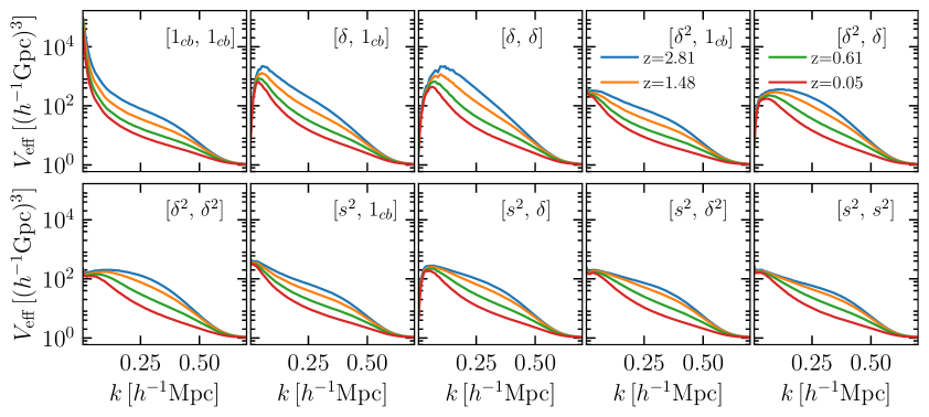
Figure 7: Effective volume for our HEFT spectrum measurements after applying ZCV. The asymptote to $(1.05h^{-1}\rm Gpc)^{3}$ at $k>0.6$ is due to the damping that we apply to $\beta^{*}$. We do not show spectra computed with the total matter field, as the results are nearly identical to the analogous spectra using the $\delta_{cb}$ field.

6 Surrogate model construction and performance

6.1 Surrogate model methodology

Having measured HEFT spectra for all of our simulations and reduced their variance using ZCV, we now proceed to construct surrogate models for them. We generally follow the surrogate modeling methodology described in [63], with a few notable changes which we highlight when described. The quantities that we emulate are not the basis spectra, $P_{ij}$, but rather the logarithm of the ratio of these spectra to their 1-loop LPT counterparts:

$$\Gamma^{ij}(k,\mathbf{\Omega})=\lg\bigg{[}\frac{P^{\rm HEFT}_{ij}(k,\mathbf{\Omega})}{P^{\rm 1\textrm{-}loop}_{ij}(k,\mathbf{\Omega})}\bigg{]}\,$$ (6.1)

where $\mathbf{\Omega}$ is a set of $w\nu$CDM cosmological parameters and $\sigma_{8}(z)$. We have empirically found that using $\sigma_{8}(z)$ instead of redshift or scale factor as a time variable significantly improves the performance of our surrogate models. Before taking the logarithm of the ratio of the HEFT and 1-loop LPT spectra, we apply a third-order Savitsky-Golay filter to the ratio with a window length of 11 in order to remove additional variance. We have tested that this smoothing procedure does not lead to any appreciable bias.

Importantly, and differently from [63], we do not use standard convolutional Lagrangian effective field theory (CLEFT) [116] predictions for $P^{\rm 1\textrm{-}loop}_{ij}(k,\ln a,\Omega)$, but rather infrared (IR) re-summed “k-expanded” CLEFT (KECLEFT), where the long-wavelength displacement correlators $A_{ij}$ are expanded in a Taylor series as described in Appendix E of [117]. Because $A_{ij}$ is Taylor expanded rather than exponentiated directly, we are able to avoid damping the linear power spectrum that goes into these terms, leading to KECLEFT predicting additional power at small scales compared to CLEFT. This additional power in KECLEFT predictions leads to more stable ratios at high-$k$ in eq. 6.1 than those derived using CLEFT, thus reducing the dynamic range in $\Gamma^{ij}$ that we must emulate. Using CLEFT instead of KECLEFT, while leaving all other choices the same leads to factors of two or more degradation in surrogate model errors.

Figure 8 shows ratios of the HEFT basis spectra to their 1-loop LPT counterparts. On large scales, the spectra converge to one another, indicating that the HEFT spectra are equivalent to 1-loop LPT predictions on these scales. In particular, $P_{cb,cb}$ matches the 1-loop LPT prediction nearly perfectly on the largest scales plotted here, indicating that our simulations recover linear growth to significantly sub-percent accuracy. Notably, HEFT spectra involving cubic combinations of fields, such as $P_{s^{2},{cb}}$, do not converge to their LPT counterparts over the range of scales that are measurable in our simulations. The residuals between HEFT and LPT spectra in these cases take the form of $\alpha k^{2}P_{cb,cb}$, where $\alpha$ is a free coefficient. This is the same form as the derivative bias spectra, $P_{\nabla^{2},cb}$, indicating that the differences in these spectra stem from differences in the smoothing conventions employed in our simulated measurements and the LPT predictions, due to our choice to implicitly smooth our predictions at the scale of the initial conditions grid. In Figure 8 we have included this extra $\alpha k^{2}P_{cb,cb}$ in the cubic 1-loop LPT predictions. Because we always include these derivative bias operators in our predictions when fitting observational data, the differences between the large scale behavior of these spectra are unimportant when interpreting data.

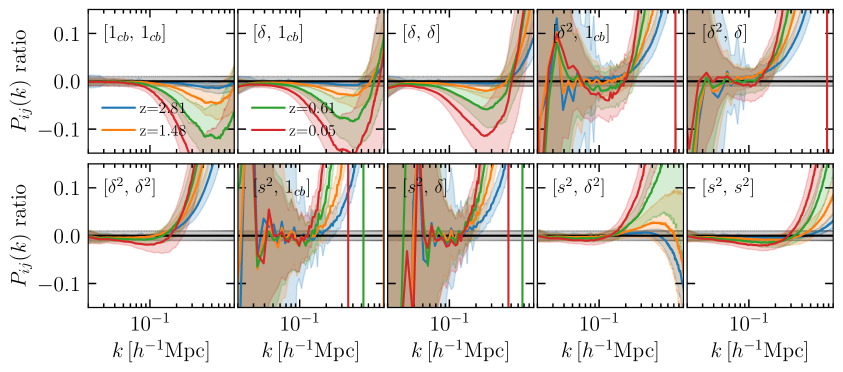
Figure 8: Fractional deviation of HEFT basis spectra from 1-loop LPT predictions, i.e. $P_{ij}^{\rm HEFT}/P_{ij}^{\rm 1-loop}-1$. Solid lines represent the means, and shaded regions are one sigma errors, while different colors represent different redshifts. On large scales, the spectra agree nearly perfectly. For spectra depending on cubic combinations of fields, e.g. $P_{s^{2},cb}$, we have included an additional term proportional to $k^{2}P_{cb,cb}(k)$ in order to bring HEFT and 1-loop LPT spectra into agreement on large scales. The need to do this stems from the different smoothing conventions used in our simulations and 1-loop LPT predictions.

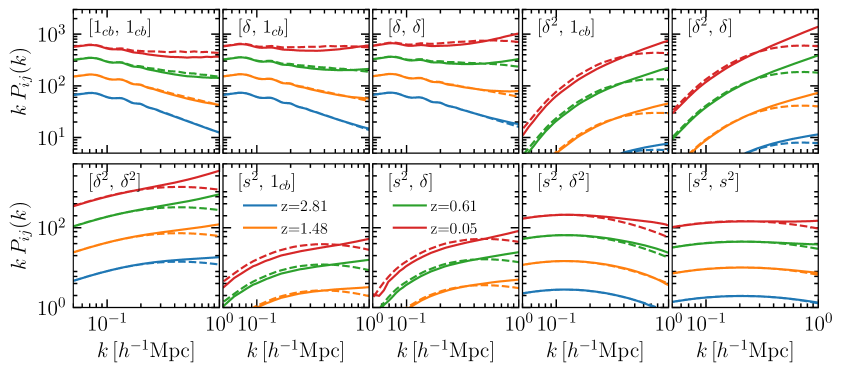
Figure 9: Predictions from our HEFT surrogate model (solid), compared with their analogous 1-loop LPT predictions (dashed). The combination of our ZCV procedure and the use of PCA in our surrogate model leads to nearly noiseless model predictions.

After measuring $\Gamma^{ij}$ for each snapshot, we perform a principal component analysis (PCA) decomposition. We employ PCA as we wish to reduce the dimensionality of our surrogate modeling problem. We construct the $N\times M$ matrix, $\mathbf{X}^{ij}$, where

$$X^{ij}_{\alpha\beta}=\Gamma^{ij}(k_{\beta},\mathbf{\Omega}_{\alpha})-\langle\Gamma^{ij}(k_{\beta})\rangle\,,$$ (6.2)

where $N=N_{\rm sim}\times N_{\rm snap}$, where $N_{\rm sim}$ is the number of simulations, 150, and $N_{\rm snap}$ is the number of snapshots per simulation, 30, and $M$ is the number of wavenumbers in our measurements of $\Gamma^{ij}$. $\mathbf{\Omega}_{\alpha}$ is a vector containing the cosmology and $\sigma_{8}(z)$ value for one of our simulation snapshots. The average in the last term on the right hand side of eq. 6.2 is taken over all cosmologies and redshifts in our training set. For $P_{m,m}$, $P_{m,cb}$ and $P_{cb,cb}$ we perform a PCA on wavenumbers between $k_{\rm min}=0.05\,\,h{\rm Mpc}^{-1}$ and $k_{\rm max}=4\,\,h{\rm Mpc}^{-1}$, giving $M=659$, while for the rest of the spectra we take $k_{\rm max}=1\,\,h{\rm Mpc}^{-1}$, where $M=159$. $P_{m,m}$, $P_{m,cb}$ and $P_{cb,cb}$ are relevant for cosmic shear and intrinsic alignment predictions, and so predictions between $k=1\,\,h{\rm Mpc}^{-1}$ and $k=4\,\,h{\rm Mpc}^{-1}$ are useful, while the rest of the spectra are only used in the Lagrangian bias expansion, which we expect to break down significantly before $k=1\,\,h{\rm Mpc}^{-1}$ and so there is no reason to emulate beyond this. Additionally, we have found that $\Gamma^{ij}$ becomes numerically unstable for $k>1\,h{\rm Mpc}^{-1}$, further motivating our choice to set $k_{\rm max}=1\,h{\rm Mpc}^{-1}$ for everything other than $P_{m,m}$, $P_{m,cb}$ and $P_{cb,cb}$. The principal components (PCs) are then given by

$$\mathbf{C}^{ij} =(\mathbf{X}^{ij})^{T}\mathbf{X}^{ij}$$

$$=(\mathbf{W}^{ij})^{T}\mathbf{\Lambda}^{ij}\mathbf{W}^{ij}\,$$

where $\mathbf{W}^{ij}$ is an $M\times M$ array whose rows are the eigenvectors that we will use, i.e. $W^{ij}_{\alpha\beta}=\textrm{PC}_{\alpha}(k_{\beta})$, and $\mathbf{\Lambda}^{ij}$ are the corresponding eigenvalues. By keeping a subset of $N_{\rm PC}$ of these PCs, we can further reduce the noise on our final predictions without decreasing their accuracy. We have found that the error incurred by truncating at $N_{\rm PC}=20$ is less than $0.1\%$, and so we use $N_{\rm PC}=20$ for the duration of this work. This is notably higher than what was required in [63], where we used 2 PCs. The need for more PCs in this work is driven both by the larger range in scales that we emulate here, as well as the significantly broader range in cosmology and redshift in the Aemulus $\nu$ simulations. We then project all $\Gamma^{ij}$ onto these PCs:

$$\mathbf{A}^{ij}=\mathbf{X}^{ij}\mathbf{W}^{ij}\,,$$ (6.3)

such that

$$\Gamma^{ij}(k_{\beta},\mathbf{\Omega}_{\alpha})=A^{ij}_{\alpha\gamma}W^{ij}_{\gamma\beta}+\langle\Gamma^{ij}(k_{\beta})\rangle\,.$$

The remaining task is to construct surrogate models, $\tilde{A}^{ij}_{\gamma}$, for the cosmology and redshift dependence of the first $N_{\rm PC}$ PC coefficients, $A^{ij}_{\alpha\gamma}$, such that

$$A^{ij}_{\alpha\gamma}\simeq\tilde{A}^{ij}_{\gamma}(\mathbf{\Omega_{\alpha}})\,.$$ (6.4)

We will use polynomial chaos expansions (PCEs) [118] as our model for $\tilde{A}^{ij}_{\gamma}$. A PCE of order $p$ is an expansion in orthonormal polynomials:

$$\tilde{A}(\mathbf{\Omega}) =\sum_{|\mathbf{\beta}|\leq p}\eta_{\mathbf{\beta}}\Psi_{\mathbf{\beta}}(\mathbf{\Omega})$$ (6.5)

where $\mathbf{\beta}\in\mathbb{N}^{D}$, and $D$ is the dimensionality of the domain of $\tilde{A}$. In our case $D=7+1$, as we have $\mathbf{\Omega}=\{\omega_{b},\omega_{c},w,n_{s},10^{9}A_{s},H_{0},\sum m_{\nu},\sigma_{8}(z)\}$. The independent variables in our problem are uncorrelated and uniformly distributed (other than $\sum m_{\nu}$), so we can use the Stieltjes three-term recurrence relation [119] to construct orthonormal polynomials, $\psi_{\beta_{i}}(\Omega_{i})$, of order $\beta_{i}$ in each variable independently. In practice we scale each parameter $\Omega_{i}$ such that $\Omega_{i}\in[-1,1]$, and so this recurrance relation yields functions that are proportional to the Legendre polynomials, i.e. $\psi_{\beta_{i}}(\Omega_{i})\propto P_{\beta_{i}}(\Omega_{i})$, where $P_{\beta_{i}}$ is the order $\beta_{i}$ Legendre polynomial. $\Psi_{\mathbf{\beta}}$ is then given by

$$\Psi_{\mathbf{\beta}}(\mathbf{\Omega})=\prod_{i=1}^{D}\psi_{\beta_{i}}(\Omega_{i})\,,$$ (6.6)

and we obtain the final expression for our surrogate models:

$$\tilde{\Gamma}^{ij}(k_{\alpha},\mathbf{\Omega}) =\tilde{A}^{ij}_{\gamma}(\mathbf{\Omega})W^{ij}_{\gamma\alpha}+\langle\Gamma^{ij}(k_{\alpha})\rangle$$ (6.7)

$$=\eta^{ij}_{\gamma\beta}\Psi_{\beta}(\mathbf{\Omega})W^{ij}_{\gamma\alpha}+\langle\Gamma^{ij}(k_{\alpha})\rangle\,.$$ (6.8)

We then use least-squares regression to fit for $\eta^{ij}_{\gamma\beta}$ given a chosen maximum order $p$. We perform these fits using the chaospy [120] python package.

In order to optimize our choice of $p$, we minimize a suitably defined measurement of the generalization error of our surrogate models. For this work we use

$$\epsilon_{ij}^{\rm max}=\mathrm{Var}\bigg{[}\operatornamewithlimits{max}\limits_{k,z}\frac{P_{ij}(k,z,\mathbf{\Omega})-\tilde{P}_{ij}(k,z,\mathbf{\Omega})}{P_{ij}(k,z,\mathbf{\Omega})}\bigg{]}\,$$ (6.9)

i.e. the variance of the maximum error taken over all $k$ and $z$ of our surrogate model $\tilde{P}_{ij}$. Since we do not have a separate suite of simulations on which to evaluate this error, we instead use a cross-validation approach, leaving one simulation out of our training set at a time, computing the error on the simulation that has been left out, and using that to evaluate eq. 6.9. We then perform a grid search over $1\leq p_{i}\leq 7$, independently for each input parameter. The resulting best fit polynomial order is $\mathbf{p}=\{2,3,3,2,2,3,2,6\}$.

Figure 9 shows the predictions from our surrogate model compared to the corresponding 1-loop LPT predictions as a function of redshift. The main notable features are that the HEFT predictions asymptote to the 1-loop LPT predictions at low $k$, and that there is no discernible residual noise on our simulation predictions.

6.2 Surrogate model performance

Figures 10 and 11 summarize the performance of our surrogate models after performing the optimization procedure described in the previous section. Figure 10 shows the one-sigma leave-one-out error evaluated for the more restrictive parameter space Tier 2 simulations as a function of $k$ and $z$ for each basis spectrum. We do not plot spectra that include the $\delta_{m}$ field, as they exhibit nearly identical behavior to their $\delta_{cb}$ counterparts. Note, that we still train on the full set of Tier 1 and Tier 2 simulations in this case. The bottom triangle depicts the fractional error for each basis spectrum, and the top triangle shows the contribution of that fractional error to a tracer auto-power spectrum with $b_{1}=1$, $b_{2}=0.2$, $b_{s}=0.2$, and $\bar{n}=5\times 10^{-4}\,h^{3}\rm Mpc^{-3}$. The errors are significantly below one percent for most redshifts, other than for spectra including the $s^{2}$ field. For reasonable choices of $b_{s}$, these terms are typically small, and so $2\%$ errors in these spectra contribute at the $<0.01\%$ level to tracer auto-power predictions, as can be seen in the upper triangle. Figure 11 shows the same thing, but evaluated over both the Tier 1 and Tier 2 simulations. The trends remain the same, but with approximately $50\%$ worse performance in the broader parameter space. We emphasize that much of this parameter space is already significantly ruled out, and we include it when constructing surrogate models in order to stabilize their performance around the edges of the parameter space allowed by current data.

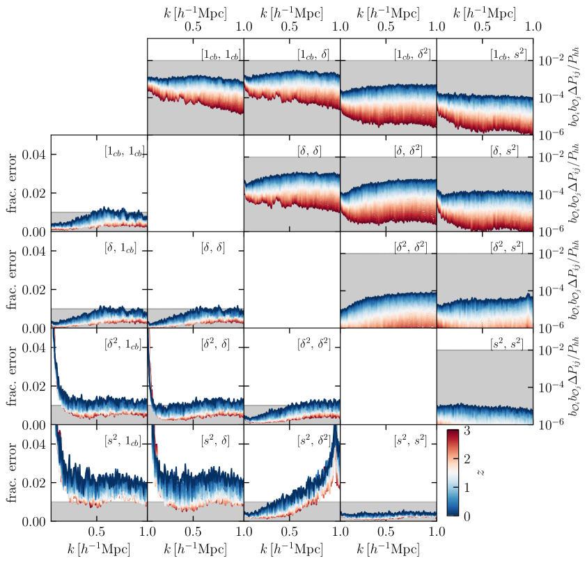
Figure 10: (lower triangle) Leave-one-out 68th percentile fractional error of our surrogate model for each basis spectrum evaluated over the tier 2 simulations. Lines are color coded by redshift, going from red to blue from $z=3$ to $z=0$. The shaded grey region shows 1% errors; most of the statistics and redshifts fall below this error threshold. We note that this cannot be directly compared to figure 5 of [63], as there we quoted errors in terms of median absolute deviation (MAD) from our simulation measurements. The surrogate model presented in this work is more accurate than that of [63] in terms of MAD. (upper triangle) Same as for the lower triangle, but now quoted in terms of the fractional error contribution to $P_{hh}$, assuming $b_{1}=1$, $b_{2}=0.2$, $b_{s}=0.2$, and $\bar{n}=5\times 10^{-4}\,h^{3}\rm Mpc^{-3}$.

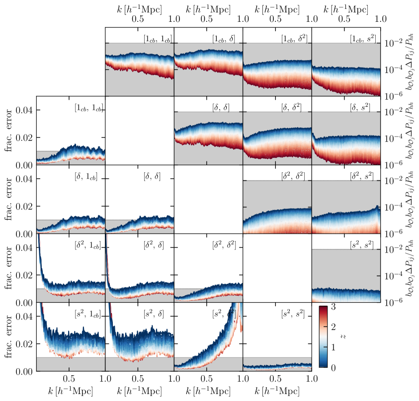
Figure 11: Same as Figure 10, but now evaluated over the entire simulation suite. The broader range in cosmologies results in approximately $50\%$ larger error.

Figure 12 shows the performance of our surrogate model for $P_{m,m}$ compared to three other state-of-the-art models: HMCode2020 [95], CosmicEmu [55] and EuclidEmu2 [54]. The top row of the figure depicts the 68th percentile error of each model compared to the Aemulus $\nu$ Tier 2 simulations where lines are color coded by their redshift, while the bottom panel shows errors for individual simulations at $z=0.53$. This redshift was chosen to be close to the peak of the galaxy-lensing kernel for upcoming galaxy-weak-lensing surveys. The performance of our $P_{m,m}$ and $P_{m,cb}$ surrogate models are quite comparable to the performance of the $P_{cb,cb}$ surrogate in Figure 10, with slightly degraded performance above $k=1\,\,h{\rm Mpc}^{-1}$.

We see that the HMCode2020 model has a 68th percentile error for $z\leq 2$ close to the $2.5\%$ error quoted in [95]. EuclidEmu2 and CosmicEmu have a relatively smaller 68th percentile error, peaking at about $2\%$ at $k=1\,\,h{\rm Mpc}^{-1}$ and staying relatively constant with redshift. The error increases significantly at the highest $k$ and $z$ shown in this figure, likely due to insufficient resolution in our simulations at these high redshifts and wavenumbers. At low wavenumbers, the CosmicEmu predictions disagree with our simulations, and linear theory at the $\sim 1-1.5\%$ level. There is also residual sample variance at the $1\%$ level discernible between $0.1\,\,h{\rm Mpc}^{-1}\leq k\leq 0.5\,\,h{\rm Mpc}^{-1}$ at low redshifts in the EuclidEmu2 model, where the paired and fixed amplitude simulations they employ remove less sample variance from their measurements than our ZCV technique. Although not plotted here, we find that EuclidEmu2 gives a 50th percentile error of about $1\%$ at $k\sim 1\,\,h{\rm Mpc}^{-1}$ and above, roughly consistent with the statistics quoted in [54]. We note that for CosmicEmu and EuclidEmu2 only 18 and 27 of our tier 2 simulations are within their training domain, respectively, and CosmicEmu does not make predictions for $z>2.02$. HMCode2020 fares significantly worse than CosmicEmu, EuclidEmu2 and our surrogate model in the quasi-linear regime, due to well studied issues in halo models at $k$ ranges that bridge the one- and two-halo regimes [121].

The black solid and dashed lines show the change in the matter power spectrum for a change of $\delta\sum m_{\nu}=0.03\,\rm eV$ and $\delta w=0.025$ away from the Planck 2018 best fit cosmology. Given the errors on our surrogate model, we would be able to distinguish these changes, whereas the other models considered would not be able to tell these apart from surrogate modeling errors. The $\delta\sum m_{\nu}=0.03\,\rm eV$ is particularly relevant, because cosmological constraints must achieve $\sigma(\sum m_{\nu})=0.03\,\rm eV$ in order to conclusively distinguish the normal and inverted mass hierarchies (e.g. [122, 123]).

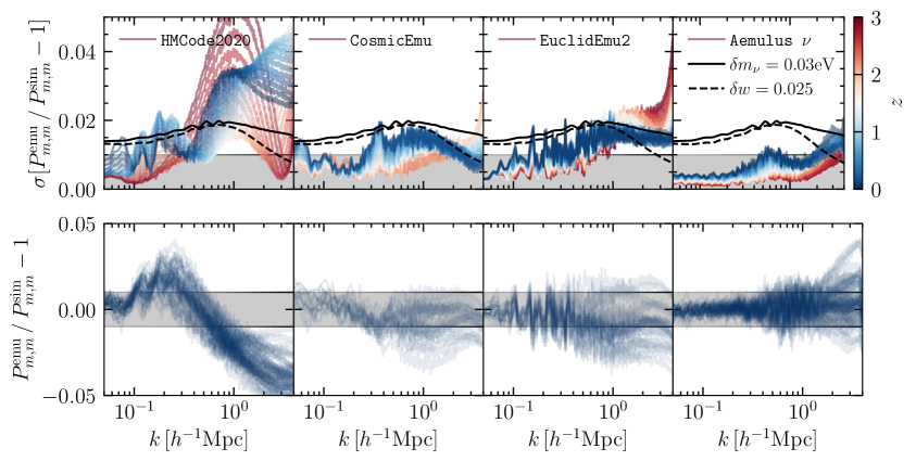
Figure 12: (Top) 68th percentile fractional error of HMCode2020 (left) CosmicEmu (middle left) EuclidEmu2 (middle right) and the matter power spectrum surrogate model presented in this work (right) to our tier 2 simulations. For Aemulus $\nu$ we use leave-one-out errors. The black solid and dashed lines show the change in the matter power spectrum for a change of $\delta\sum m_{\nu}=0.03\,\rm eV$ and $\delta w=0.025$ away from the Planck 2018 best fit cosmology. (Bottom) Fractional error at $z=0.53$ for each of our tier 2 simulations. For CosmicEmu and EuclidEmu2 we only compare to 18 and 27 of our tier 2 simulations that are in their domains, respectively. None of the models exhibit significant outliers in their performance compared to the 68th percentile errors shown in the top panels. The performance of Aemulus $\nu$ becomes slightly more unstable above $k=1\,\,h{\rm Mpc}^{-1}$, with a few $2-3\%$ outliers apparent.

6.3 Error modeling

Although this performance satisfies our goals of $\leq 2\%$ 68th percentile error over our full parameter space, and $\leq 1\%$ 68th percentile error in our tier 2 parameter space, the errors on our surrogates may not be entirely negligible for all analyses. In particular, as shown in Figure 13, the errors have correlations as a function of scale that may contribute significantly to otherwise small off-diagonal elements of covariance matrices. To facilitate the incorporation of these errors into analyses, we provide additional functionality to produce covariance matrices of these fractional errors for each basis spectrum along with our trained surrogate models. In particular, we measure the following quantity:

$$\textrm{Cov}\left[\epsilon_{i,j}(k),\epsilon_{l,m}(k^{\prime})\right]=\sum_{n=0}^{N_{\rm sim}}(\epsilon_{i,j}^{n}(k)-\bar{\epsilon}_{i,j}(k))(\epsilon_{l,m}^{n}(k^{\prime})-\bar{\epsilon}_{l,m}(k^{\prime}))\,,$$ (6.10)

where

$$\epsilon_{i,j}^{n}(k)=\frac{P_{ij}(k,z,\mathbf{\Omega}^{n})-\tilde{P}^{n}_{ij}(k,z,\mathbf{\Omega}^{n})}{P_{ij}(k,z,\mathbf{\Omega}^{n})}\,$$ (6.11)

is the fractional error for simulation $n$ in our suite and $\tilde{P}^{n}_{ij}(k,z,\mathbf{\Omega}^{n})$ is the emulator prediction trained on all simulations except for the $n$th one. We can then compute errors on $P_{gg}$ assuming bias parameters $b_{i}$ as

$$\textrm{Cov}^{\rm emu}\left[P_{gg}(k),P_{gg}(k^{\prime})\right]=\sum_{i,j,l,m}b_{i}b_{j}b_{l}b_{m}P_{i,j}(k)P_{l,m}(k^{\prime})\textrm{Cov}\left[\epsilon_{i,j}(k),\epsilon_{l,m}(k^{\prime})\right]\,$$ (6.12)

and this covariance can then be further integrated along the line of sight, via e.g. the Limber approximation, to produce emulator error contributions to the covariances of angular power spectra. One such prediction for a DESI-like sample is used in Figure 1.

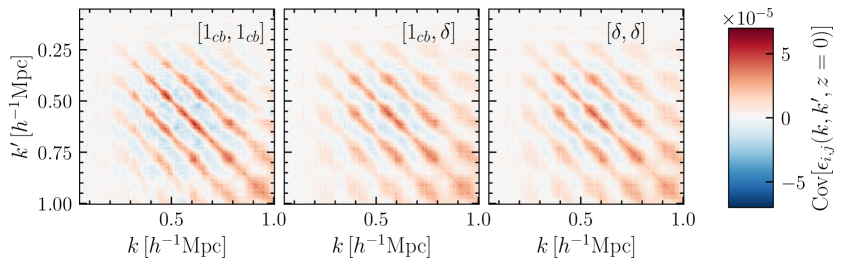
Figure 13: Covariance of the fractional error of our $P_{cb,cb}$, $P_{cb,\delta}$ and $P_{\delta,\delta}$ surrogate models at $z=0$. Significant off-diagonal structure is present, although the amplitude of the overall errors are small. Our surrogate modeling code provides an interface to these covariances so that they can be appropriately accounted for when using the models presented in this work in data analysis.

7 Summary

In this work, we have introduced the Aemulus $\nu$ suite, a set of 150 $N$-body simulations in a $w\nu$CDM parameter space that evolve massive neutrinos as an additional particle species. The $w\nu$CDM cosmological parameter space of these simulations is sufficiently broad to make them useful for investigating tensions between cosmological constraints coming from large scale structure and cosmic microwave background experiments. Along with these simulations, we present new hybrid effective field theory (HEFT) and matter power spectrum surrogate models that represent significant improvements over the current state of the art.

In Section 2 we describe how the sampling of $w\nu$CDM parameter space was optimized in order to simultaneously maximize parameter space breadth while maintaining surrogate model accuracy. To do so, we constructed surrogate models for HMCode2020 matter power spectrum predictions, varying the allowed boundaries of our parameter space. Using these surrogate models, we found that a two-tiered design, with 100 simulations in a broad $w\nu$CDM parameter space, and 50 simulations in a parameter space with bounds restricted to be closer to currently preferred constraints, yielded an accuracy that met our requirements.

In Section 3, we describe the settings that were used to run our simulations, the simulation convergence tests that we performed. We use a modified version of Gadget3 to evolve $1400^{3}$ CDM and neutrino particles (for a total of $2\times 1400^{3}$ particles) in a $(1.05h^{-1}\rm Gpc)^{3}$ volume, yielding a $cb$ particle mass of $3.51\times 10^{10}\frac{\Omega_{cb}}{0.3}~{}h^{-1}M_{\odot}$. In order to mitigate systematic errors associated with early simulation starting times, we initialize our simulations at $z=12$ using third order Lagrangian perturbation theory (3LPT) as implemented in a modified version of monofonic . As this is a significant change from previous simulations run as part of the Aemulus project, we perform convergence tests demonstrating that starting at $z_{\rm ini}=12$ is converged at the $\leq 1\%$ level with respect to a simulation run with four times the number of particles, starting at $z_{\rm ini}=24$.

Section 4 introduces relevant perturbation theory notation, and describes how we measure HEFT basis spectra from our simulations. Then, in Section 5, we describe our Zel’dovich control variate (ZCV) methodology, showing that it reduces the sample variance on HEFT spectra to the equivalent errors that we would obtain by running $10-10^{5}$ times larger simulations, depending on the basis spectrum and scale in question. Doing so leads to extremely smooth predictions from our surrogate models, outperforming the improvements obtained from paired and fixed simulations, and allowing us to run more simulations than we would have otherwise been able to while still meeting our accuracy requirements. We believe the ZCV technique will play an important role in similar applications in the future.

We described the implementation and optimization of our combined principal component analysis (PCA) and polynomial chaos expansion (PCE) surrogate models in Section 6. There, we demonstrated that our HEFT surrogate model achieves $\leq 1\%$ 68th percentile error for most basis spectra over our Tier 2 parameter space and $\leq 2\%$ 68th percentile error over our full parameter space for $k\leq 1\,h{\rm Mpc}^{-1}$ and $0\leq z\leq 3$. The basis spectra that exceed these error thresholds are sub-dominant, and thus their slightly worse accuracy is not of great concern. Our matter power spectrum surrogate model achieves $\leq 1\%$ 68th percentile error over our tier 2 simulations out to $k=1\,h{\rm Mpc}^{-1}$ and $\leq 2\%$ 68th percentile error for $1\,h{\rm Mpc}^{-1}<k\leq 4\,h{\rm Mpc}^{-1}$. We compare our matter power spectrum model to HMCode2020 , CosmicEmu and EuclidEmu2 , finding that our model outperforms them when evaluated on the tier 2 Aemulus $\nu$ simulations. We also provide estimates of surrogate model error covariance as a function of redshift along with our trained surrogate models so that it may be incorporated as a theory error in analyses using our models.

We anticipate that the HEFT model presented here will be useful for analyses of projected galaxy clustering and weak lensing for many future surveys. This model can straight-forwardly replace 1-loop LPT models for these statistics, extending their reach in scale by a factor of two to three. HEFT can also serve as an immediate upgrade in terms of model flexibility and accuracy for analyses that currently use non-linear matter power spectra and constant linear bias. The matter power spectrum model presented here is the most accurate to date, and can play a vital role in stage III and stage IV analyses of weak lensing auto-spectra. We have made these models available at https://github.com/AemulusProject/aemulus_heft. We will also make halo catalogs and downsampled particle catalogs available at https://github.com/AemulusProject/aemulus_nu_public upon publication of this work, and full snapshot data will be made available upon request to the authors. In future work we will also release new halo mass function and halo bias models based on the simulations presented here.

Appendix A HMcode2020 surrogate model error

In this appendix we discuss the accuracy of the HMCode2020 surrogate model trained on the same cosmologies used to run the Aemulus $\nu$ simulations. In order to train our HMCode2020 surrogate model we use the same optimization procedure described in Section 6. In Figure 14 we compare the resulting HMCode2020 68th percentile surrogate model error taken over all cosmologies and redshifts to that obtained using the Aemulus $\nu$ simulations. The errors for the HMCode2020 model are evaluated on the independent set of 10,000 HMCode2020 predictions sampled using a Sobol sequence [100] over the Tier 1 cosmology space, while the Aemulus $\nu$ errors are computed using the leave-one-out cross-validation procedure described in Section 6. For $k>0.3\,\,h{\rm Mpc}^{-1}$ the errors are quite comparable to each other both for the Tier 2 cosmologies (blue) and the full set of cosmologies (orange). At lower $k$ values than this, the Aemulus $\nu$ errors are notably larger, likely due to residual sample variance in our simulation measurements.

Because we have a dense set of HMCode2020 test models, we can accurately measure the cosmology dependence of our surrogate model error. Given that the cosmology averaged 68th percentile errors are comparable between our HMCode2020 and Aemulus $\nu$ models, we can hope that the cosmology dependence of the errors are also similar. Figure 15 shows the 68th percentile fractional error, taken over cosmology and redshift, at $k=1\,\,h{\rm Mpc}^{-1}$ as a function of cosmology for our HMCode2020 surrogate model. The black lines represent the bounds of the Tier 2 parameter space. Within this region the error is very stable and almost always below $1\%$. Beyond this, the error monotonically increases, with some excursions beyond $2\%$ at the edges of our parameter space in $w$, $\omega_{c}$ and $H_{0}$.

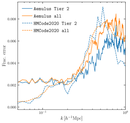
Figure 14: Comparison between 68th percentile fractional residuals, averaged over all redshifts, of our HMCode2020 $P_{m,m}$ surrogate model (dashed) and Aemulus $\nu$ surrogate model (solid), when both are trained using our fiducial parameter space design. For the HMCode2020 model, errors are evaluated using a set of 10,000 cosmologies generated over the Tier 1 parameter space, while errors for the Aemulus $\nu$ model are evaluated using the leave-one-out methodology described in Section 6. Blue lines are errors measured in the Tier 2 parameter space, while orange lines are evaluated over the full Tier 1 parameter space. The errors are quite comparable between the model built on HMCode2020 data compared to that built from our actual Aemulus $\nu$ simulations, except at $k\leq 0.2\,\,h{\rm Mpc}^{-1}$, where residual sample variance may be contributing additional variance to the Aemulus $\nu$ based model.

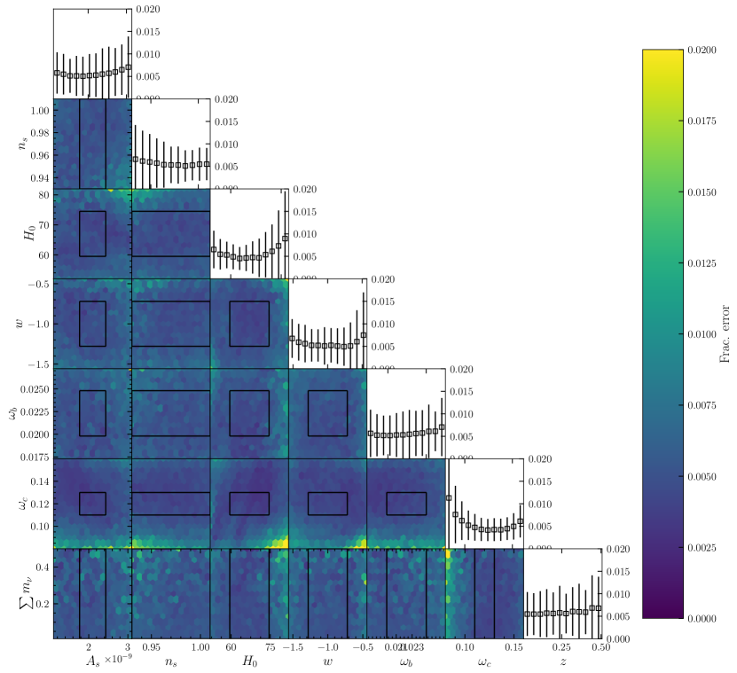
Figure 15: 68th percentile fractional error at $k=1\,\,h{\rm Mpc}^{-1}$ evaluated for the HMCode2020 $P_{m,m}$ surrogate model trained on our fiducial parameter space design, and tested on a set of 10,000 cosmologies in the Tier 1 parameter space drawn from a Sobol sequence. The black boxes represent the boundaries of the Tier 2 parameter space. The points with error bars are the one-dimensional marginal mean fractional errors with 1-sigma errors.

References

- [1] G. d’Amico, J. Gleyzes, N. Kokron, K. Markovic, L. Senatore, P. Zhang et al., The cosmological analysis of the SDSS/BOSS data from the Effective Field Theory of Large-Scale Structure, Journal of Cosmology and Astro-Particle Physics 2020 (2020) 005 [1909.05271].
- [2] M.M. Ivanov, M. Simonović and M. Zaldarriaga, Cosmological parameters from the BOSS galaxy power spectrum, Journal of Cosmology and Astro-Particle Physics 2020 (2020) 042 [1909.05277].
- [3] S.-F. Chen, Z. Vlah, E. Castorina and M. White, Redshift-space distortions in Lagrangian perturbation theory, Journal of Cosmology and Astro-Particle Physics 2021 (2021) 100 [2012.04636].
- [4] O.H.E. Philcox, M.M. Ivanov, G. Cabass, M. Simonović, M. Zaldarriaga and T. Nishimichi, Cosmology with the redshift-space galaxy bispectrum monopole at one-loop order, Phys. Rev. D 106 (2022) 043530 [2206.02800].
- [5] G. D’Amico, Y. Donath, M. Lewandowski, L. Senatore and P. Zhang, The BOSS bispectrum analysis at one loop from the Effective Field Theory of Large-Scale Structure, arXiv e-prints (2022) arXiv:2206.08327 [2206.08327].
- [6] G. D’Amico, Y. Donath, M. Lewandowski, L. Senatore and P. Zhang, The one-loop bispectrum of galaxies in redshift space from the Effective Field Theory of Large-Scale Structure, arXiv e-prints (2022) arXiv:2211.17130 [2211.17130].
- [7] M. Lewandowski, A. Maleknejad and L. Senatore, An effective description of dark matter and dark energy in the mildly non-linear regime, Journal of Cosmology and Astro-Particle Physics 2017 (2017) 038 [1611.07966].
- [8] L. Senatore and M. Zaldarriaga, The Effective Field Theory of Large-Scale Structure in the presence of Massive Neutrinos, arXiv e-prints (2017) arXiv:1707.04698 [1707.04698].
- [9] A. Aviles and A. Banerjee, A Lagrangian perturbation theory in the presence of massive neutrinos, Journal of Cosmology and Astroparticle Physics 2020 (2020) 034 [2007.06508].
- [10] A. Aviles, G. Valogiannis, M.A. Rodriguez-Meza, J.L. Cervantes-Cota, B. Li and R. Bean, Redshift space power spectrum beyond Einstein-de Sitter kernels, Journal of Cosmology and Astro-Particle Physics 2021 (2021) 039 [2012.05077].
- [11] S.-F. Chen, Z. Vlah and M. White, A new analysis of galaxy 2-point functions in the BOSS survey, including full-shape information and post-reconstruction BAO, Journal of Cosmology and Astroparticle Physics 2022 (2022) 008 [2110.05530].
- [12] S. Foreman, H. Perrier and L. Senatore, Precision comparison of the power spectrum in the EFTofLSS with simulations, Journal of Cosmology and Astro-Particle Physics 2016 (2016) 027 [1507.05326].
- [13] T. Nishimichi, G. D’Amico, M.M. Ivanov, L. Senatore, M. Simonović, M. Takada et al., Blinded challenge for precision cosmology with large-scale structure: Results from effective field theory for the redshift-space galaxy power spectrum, Phys. Rev. D 102 (2020) 123541 [2003.08277].
- [14] V. Springel, R. Pakmor, O. Zier and M. Reinecke, Simulating cosmic structure formation with the GADGET-4 code, Mon. Not. R. Astron. Soc. 506 (2021) 2871 [2010.03567].
- [15] L.H. Garrison, D.J. Eisenstein, D. Ferrer, N.A. Maksimova and P.A. Pinto, The ABACUS cosmological N-body code, Mon. Not. R. Astron. Soc. 508 (2021) 575 [2110.11392].
- [16] D. Potter, J. Stadel and R. Teyssier, PKDGRAV3: beyond trillion particle cosmological simulations for the next era of galaxy surveys, Computational Astrophysics and Cosmology 4 (2017) 2 [1609.08621].
- [17] S. Habib, A. Pope, H. Finkel, N. Frontiere, K. Heitmann, D. Daniel et al., HACC: Simulating sky surveys on state-of-the-art supercomputing architectures, New Astronomy 42 (2016) 49 [1410.2805].
- [18] J. Brandbyge and S. Hannestad, Grid based linear neutrino perturbations in cosmological N-body simulations, Journal of Cosmology and Astro-Particle Physics 2009 (2009) 002 [0812.3149].
- [19] Y. Ali-Haïmoud and S. Bird, An efficient implementation of massive neutrinos in non-linear structure formation simulations, Mon. Not. R. Astron. Soc. 428 (2013) 3375 [1209.0461].
- [20] E. Castorina, C. Carbone, J. Bel, E. Sefusatti and K. Dolag, DEMNUni: the clustering of large-scale structures in the presence of massive neutrinos, Journal of Cosmology and Astroparticle Physics 2015 (2015) 043 [1505.07148].
- [21] A. Upadhye, J. Kwan, A. Pope, K. Heitmann, S. Habib, H. Finkel et al., Redshift-space distortions in massive neutrino and evolving dark energy cosmologies, Phys. Rev. D 93 (2016) 063515 [1506.07526].
- [22] J. Adamek, R.E. Angulo, C. Arnold, M. Baldi, M. Biagetti, B. Bose et al., Euclid: Modelling massive neutrinos in cosmology – a code comparison, arXiv e-prints (2022) arXiv:2211.12457 [2211.12457].
- [23] M. Viel, M.G. Haehnelt and V. Springel, The effect of neutrinos on the matter distribution as probed by the intergalactic medium, Journal of Cosmology and Astro-Particle Physics 2010 (2010) 015 [1003.2422].
- [24] A. Banerjee and N. Dalal, Simulating nonlinear cosmological structure formation with massive neutrinos, Journal of Cosmology and Astro-Particle Physics 2016 (2016) 015 [1606.06167].
- [25] S. Bird, Y. Ali-Haïmoud, Y. Feng and J. Liu, An efficient and accurate hybrid method for simulating non-linear neutrino structure, Mon. Not. R. Astron. Soc. 481 (2018) 1486 [1803.09854].
- [26] J.M. Sullivan, J.D. Emberson, S. Habib and N. Frontiere, Improving initialization and evolution accuracy of cosmological neutrino simulations, arXiv e-prints (2023) arXiv:2302.09134 [2302.09134].
- [27] A. Banerjee, D. Powell, T. Abel and F. Villaescusa-Navarro, Reducing noise in cosmological N-body simulations with neutrinos, Journal of Cosmology and Astro-Particle Physics 2018 (2018) 028 [1801.03906].
- [28] A.E. Bayer, A. Banerjee and Y. Feng, A fast particle-mesh simulation of non-linear cosmological structure formation with massive neutrinos, Journal of Cosmology and Astro-Particle Physics 2021 (2021) 016 [2007.13394].
- [29] U. Seljak, Analytic model for galaxy and dark matter clustering, Mon. Not. R. Astron. Soc. 318 (2000) 203 [astro-ph/0001493].
- [30] A.A. Berlind and D.H. Weinberg, The Halo Occupation Distribution: Toward an Empirical Determination of the Relation between Galaxies and Mass, Astrophys. J. 575 (2002) 587 [astro-ph/0109001].
- [31] J.S. Bullock, R.H. Wechsler and R.S. Somerville, Galaxy halo occupation at high redshift, Mon. Not. R. Astron. Soc. 329 (2002) 246 [astro-ph/0106293].
- [32] B.A. Reid, H.-J. Seo, A. Leauthaud, J.L. Tinker and M. White, A 2.5 per cent measurement of the growth rate from small-scale redshift space clustering of SDSS-III CMASS galaxies, Mon. Not. R. Astron. Soc. 444 (2014) 476 [1404.3742].
- [33] J.U. Lange, A.P. Hearin, A. Leauthaud, F.C. van den Bosch, H. Guo and J. DeRose, Five per cent measurements of the growth rate from simulation-based modelling of redshift-space clustering in BOSS LOWZ, Mon. Not. R. Astron. Soc. 509 (2022) 1779 [2101.12261].
- [34] Z. Zhai, J.L. Tinker, A. Banerjee, J. DeRose, H. Guo, Y.-Y. Mao et al., The Aemulus Project V: Cosmological constraint from small-scale clustering of BOSS galaxies, arXiv e-prints (2022) arXiv:2203.08999 [2203.08999].
- [35] S. Yuan, L.H. Garrison, B. Hadzhiyska, S. Bose and D.J. Eisenstein, ABACUSHOD: a highly efficient extended multitracer HOD framework and its application to BOSS and eBOSS data, Mon. Not. R. Astron. Soc. 510 (2022) 3301 [2110.11412].
- [36] B.D. Wibking, D.H. Weinberg, A.N. Salcedo, H.-Y. Wu, S. Singh, S. Rodríguez-Torres et al., Cosmology with galaxy-galaxy lensing on non-perturbative scales: emulation method and application to BOSS LOWZ, Mon. Not. R. Astron. Soc. 492 (2020) 2872 [1907.06293].
- [37] H. Miyatake, S. Sugiyama, M. Takada, T. Nishimichi, M. Shirasaki, Y. Kobayashi et al., Cosmological inference from an emulator based halo model. II. Joint analysis of galaxy-galaxy weak lensing and galaxy clustering from HSC-Y1 and SDSS, Phys. Rev. D 106 (2022) 083520 [2111.02419].
- [38] K. Storey-Fisher, J. Tinker, Z. Zhai, J. DeRose, R.H. Wechsler and A. Banerjee, The Aemulus Project VI: Emulation of beyond-standard galaxy clustering statistics to improve cosmological constraints, arXiv e-prints (2022) arXiv:2210.03203 [2210.03203].
- [39] G. Valogiannis and C. Dvorkin, Going beyond the galaxy power spectrum: An analysis of BOSS data with wavelet scattering transforms, Phys. Rev. D 106 (2022) 103509 [2204.13717].
- [40] R. García and E. Rozo, Halo exclusion criteria impacts halo statistics, Mon. Not. R. Astron. Soc. 489 (2019) 4170 [1903.01709].
- [41] J. Tinker, A.V. Kravtsov, A. Klypin, K. Abazajian, M. Warren, G. Yepes et al., Toward a Halo Mass Function for Precision Cosmology: The Limits of Universality, Astrophys. J. 688 (2008) 709 [0803.2706].
- [42] B. Dai, Y. Feng, U. Seljak and S. Singh, High mass and halo resolution from fast low resolution simulations, Journal of Cosmology and Astro-Particle Physics 2020 (2020) 002 [1908.05276].
- [43] A.S. Villarreal, A.R. Zentner, Y.-Y. Mao, C.W. Purcell, F.C. van den Bosch, B. Diemer et al., The immitigable nature of assembly bias: the impact of halo definition on assembly bias, Mon. Not. R. Astron. Soc. 472 (2017) 1088 [1705.04327].
- [44] P. Mansfield and A.V. Kravtsov, The three causes of low-mass assembly bias, Mon. Not. R. Astron. Soc. 493 (2020) 4763 [1902.00030].
- [45] D. Nelson, V. Springel, A. Pillepich, V. Rodriguez-Gomez, P. Torrey, S. Genel et al., The IllustrisTNG simulations: public data release, Computational Astrophysics and Cosmology 6 (2019) 2 [1812.05609].
- [46] J. Schaye, R.A. Crain, R.G. Bower, M. Furlong, M. Schaller, T. Theuns et al., The EAGLE project: simulating the evolution and assembly of galaxies and their environments, Mon. Not. R. Astron. Soc. 446 (2015) 521 [1407.7040].
- [47] I.G. McCarthy, J. Schaye, S. Bird and A.M.C. Le Brun, The BAHAMAS project: calibrated hydrodynamical simulations for large-scale structure cosmology, Mon. Not. R. Astron. Soc. 465 (2017) 2936 [1603.02702].
- [48] P.F. Hopkins, A. Wetzel, D. Kereš, C.-A. Faucher-Giguère, E. Quataert, M. Boylan-Kolchin et al., FIRE-2 simulations: physics versus numerics in galaxy formation, Mon. Not. R. Astron. Soc. 480 (2018) 800 [1702.06148].
- [49] C. Modi, S.-F. Chen and M. White, Simulations and symmetries, Mon. Not. R. Astron. Soc. 492 (2020) 5754 [1910.07097].
- [50] A. Banerjee, N. Kokron and T. Abel, Modelling nearest neighbour distributions of biased tracers using hybrid effective field theory, Mon. Not. R. Astron. Soc. 511 (2022) 2765 [2107.10287].
- [51] A. Banerjee and T. Abel, Nearest neighbour distributions: New statistical measures for cosmological clustering, Mon. Not. R. Astron. Soc. 500 (2021) 5479 [2007.13342].
- [52] A. Banerjee and T. Abel, Cosmological cross-correlations and nearest neighbour distributions, Mon. Not. R. Astron. Soc. 504 (2021) 2911 [2102.01184].
- [53] K. Heitmann, D. Bingham, E. Lawrence, S. Bergner, S. Habib, D. Higdon et al., The Mira-Titan Universe: Precision Predictions for Dark Energy Surveys, Astrophys. J. 820 (2016) 108 [1508.02654].
- [54] Euclid Collaboration, M. Knabenhans, J. Stadel, D. Potter, J. Dakin, S. Hannestad et al., Euclid preparation: IX. EuclidEmulator2 - power spectrum emulation with massive neutrinos and self-consistent dark energy perturbations, Mon. Not. R. Astron. Soc. 505 (2021) 2840 [2010.11288].
- [55] K.R. Moran, K. Heitmann, E. Lawrence, S. Habib, D. Bingham, A. Upadhye et al., The Mira-Titan Universe - IV. High precision power spectrum emulation, Mon. Not. R. Astron. Soc. (2022) [2207.12345].
- [56] T. McClintock, E. Rozo, M.R. Becker, J. DeRose, Y.-Y. Mao, S. McLaughlin et al., The Aemulus Project. II. Emulating the Halo Mass Function, Astrophys. J. 872 (2019) 53 [1804.05866].
- [57] S. Bocquet, K. Heitmann, S. Habib, E. Lawrence, T. Uram, N. Frontiere et al., The Mira-Titan Universe. III. Emulation of the Halo Mass Function, Astrophys. J. 901 (2020) 5 [2003.12116].
- [58] T. McClintock, E. Rozo, A. Banerjee, M.R. Becker, J. DeRose, S. McLaughlin et al., The Aemulus Project IV: Emulating Halo Bias, arXiv e-prints (2019) arXiv:1907.13167 [1907.13167].
- [59] T. Nishimichi, M. Takada, R. Takahashi, K. Osato, M. Shirasaki, T. Oogi et al., Dark Quest. I. Fast and Accurate Emulation of Halo Clustering Statistics and Its Application to Galaxy Clustering, Astrophys. J. 884 (2019) 29 [1811.09504].
- [60] B.D. Wibking, A.N. Salcedo, D.H. Weinberg, L.H. Garrison, D. Ferrer, J. Tinker et al., Emulating galaxy clustering and galaxy-galaxy lensing into the deeply non-linear regime: methodology, information, and forecasts, Mon. Not. R. Astron. Soc. 484 (2019) 989 [1709.07099].
- [61] A.N. Salcedo, A.H. Maller, A.A. Berlind, M. Sinha, C.K. McBride, P.S. Behroozi et al., Spatial clustering of dark matter haloes: secondary bias, neighbour bias, and the influence of massive neighbours on halo properties, Mon. Not. R. Astron. Soc. 475 (2018) 4411 [1708.08451].
- [62] Z. Zhai, J.L. Tinker, M.R. Becker, J. DeRose, Y.-Y. Mao, T. McClintock et al., The Aemulus Project. III. Emulation of the Galaxy Correlation Function, Astrophys. J. 874 (2019) 95 [1804.05867].
- [63] N. Kokron, J. DeRose, S.-F. Chen, M. White and R.H. Wechsler, The cosmology dependence of galaxy clustering and lensing from a hybrid N-body-perturbation theory model, Mon. Not. R. Astron. Soc. 505 (2021) 1422 [2101.11014].
- [64] M. Zennaro, R.E. Angulo, M. Pellejero-Ibáñez, J. Stücker, S. Contreras and G. Aricò, The BACCO simulation project: biased tracers in real space, arXiv e-prints (2021) arXiv:2101.12187 [2101.12187].
- [65] M. Pellejero Ibañez, J. Stücker, R.E. Angulo, M. Zennaro, S. Contreras and G. Aricò, Modelling galaxy clustering in redshift space with a Lagrangian bias formalism and N-body simulations, Mon. Not. R. Astron. Soc. 514 (2022) 3993 [2109.08699].
- [66] M. Pellejero Ibañez, R.E. Angulo, M. Zennaro, J. Stücker, S. Contreras, G. Aricò et al., The bacco simulation project: bacco hybrid Lagrangian bias expansion model in redshift space, Mon. Not. R. Astron. Soc. 520 (2023) 3725 [2207.06437].
- [67] B. Hadzhiyska, C. García-García, D. Alonso, A. Nicola and A. Slosar, Hefty enhancement of cosmological constraints from the DES Y1 data using a hybrid effective field theory approach to galaxy bias, Journal of Cosmology and Astro-Particle Physics 2021 (2021) 020 [2103.09820].
- [68] J.A. Peacock and S.J. Dodds, Non-linear evolution of cosmological power spectra, Mon. Not. R. Astron. Soc. 280 (1996) L19 [astro-ph/9603031].
- [69] R.E. Angulo and A. Pontzen, Cosmological N-body simulations with suppressed variance, Mon. Not. R. Astron. Soc. 462 (2016) L1 [1603.05253].
- [70] A. Pontzen, A. Slosar, N. Roth and H.V. Peiris, Inverted initial conditions: Exploring the growth of cosmic structure and voids, Phys. Rev. D 93 (2016) 103519 [1511.04090].
- [71] Euclid Collaboration, M. Knabenhans, J. Stadel, S. Marelli, D. Potter, R. Teyssier et al., Euclid preparation: II. The EUCLIDEMULATOR - a tool to compute the cosmology dependence of the nonlinear matter power spectrum, Mon. Not. R. Astron. Soc. 484 (2019) 5509 [1809.04695].
- [72] R.E. Angulo, M. Zennaro, S. Contreras, G. Aricò, M. Pellejero-Ibañez and J. Stücker, The BACCO simulation project: exploiting the full power of large-scale structure for cosmology, Mon. Not. R. Astron. Soc. 507 (2021) 5869 [2004.06245].
- [73] F. Villaescusa-Navarro, S. Naess, S. Genel, A. Pontzen, B. Wandelt, L. Anderson et al., Statistical Properties of Paired Fixed Fields, Astrophys. J. 867 (2018) 137 [1806.01871].
- [74] C.-H. Chuang, G. Yepes, F.-S. Kitaura, M. Pellejero-Ibanez, S. Rodríguez-Torres, Y. Feng et al., UNIT project: Universe N-body simulations for the Investigation of Theoretical models from galaxy surveys, Mon. Not. R. Astron. Soc. 487 (2019) 48 [1811.02111].
- [75] F. Maion, R.E. Angulo and M. Zennaro, Statistics of biased tracers in variance-suppressed simulations, Journal of Cosmology and Astro-Particle Physics 2022 (2022) 036 [2204.03868].
- [76] A.B. Owen, Monte Carlo theory, methods and examples (2013).
- [77] N. Chartier, B. Wandelt, Y. Akrami and F. Villaescusa-Navarro, CARPool: fast, accurate computation of large-scale structure statistics by pairing costly and cheap cosmological simulations, Mon. Not. R. Astron. Soc. 503 (2021) 1897 [2009.08970].
- [78] N. Chartier and B.D. Wandelt, CARPool covariance: fast, unbiased covariance estimation for large-scale structure observables, Mon. Not. R. Astron. Soc. 509 (2022) 2220 [2106.11718].
- [79] N. Chartier and B.D. Wandelt, Bayesian control variates for optimal covariance estimation with pairs of simulations and surrogates, Mon. Not. R. Astron. Soc. 515 (2022) 1296 [2204.03070].
- [80] S. Tassev, D.J. Eisenstein, B.D. Wandelt and M. Zaldarriaga, sCOLA: The N-body COLA Method Extended to the Spatial Domain, arXiv e-prints (2015) arXiv:1502.07751 [1502.07751].
- [81] Y. Feng, M.-Y. Chu, U. Seljak and P. McDonald, FASTPM: a new scheme for fast simulations of dark matter and haloes, MNRAS 463 (2016) 2273 [1603.00476].
- [82] N. Kokron, S.-F. Chen, M. White, J. DeRose and M. Maus, Accurate predictions from small boxes: variance suppression via the Zel’dovich approximation, Journal of Cosmology and Astro-Particle Physics 2022 (2022) 059 [2205.15327].
- [83] J. DeRose, S.-F. Chen, N. Kokron and M. White, Precision redshift-space galaxy power spectra using Zel’dovich control variates, Journal of Cosmology and Astro-Particle Physics 2023 (2023) 008 [2210.14239].
- [84] M. White, R. Zhou, J. DeRose, S. Ferraro, S.-F. Chen, N. Kokron et al., Cosmological constraints from the tomographic cross-correlation of DESI Luminous Red Galaxies and Planck CMB lensing, Journal of Cosmology and Astro-Particle Physics 2022 (2022) 007 [2111.09898].
- [85] S.-F. Chen, M. White, J. DeRose and N. Kokron, Cosmological analysis of three-dimensional BOSS galaxy clustering and Planck CMB lensing cross correlations via Lagrangian perturbation theory, Journal of Cosmology and Astro-Particle Physics 2022 (2022) 041 [2204.10392].
- [86] C. Heymans, T. Tröster, M. Asgari, C. Blake, H. Hildebrandt, B. Joachimi et al., KiDS-1000 Cosmology: Multi-probe weak gravitational lensing and spectroscopic galaxy clustering constraints, Astron. Astrophys. 646 (2021) A140 [2007.15632].
- [87] T.M.C. Abbott, M. Aguena, A. Alarcon, S. Allam, O. Alves, A. Amon et al., Dark Energy Survey Year 3 results: Cosmological constraints from galaxy clustering and weak lensing, Phys. Rev. D 105 (2022) 023520 [2105.13549].
- [88] Planck Collaboration, N. Aghanim, Y. Akrami, M. Ashdown, J. Aumont, C. Baccigalupi et al., Planck 2018 results. VI. Cosmological parameters, Astron. Astrophys. 641 (2020) A6 [1807.06209].
- [89] LSST collaboration, LSST: from Science Drivers to Reference Design and Anticipated Data Products, Astrophys. J. 873 (2019) 111 [0805.2366].
- [90] A. Lee, M.H. Abitbol, S. Adachi, P. Ade, J. Aguirre, Z. Ahmed et al., The Simons Observatory, in Bulletin of the American Astronomical Society, vol. 51, p. 147, Sept., 2019, DOI [1907.08284].
- [91] N. Kokron, J. DeRose, S.-F. Chen, M. White and R.H. Wechsler, Priors on red galaxy stochasticity from hybrid effective field theory, Mon. Not. R. Astron. Soc. 514 (2022) 2198 [2112.00012].
- [92] R. Zhou, B. Dey, J.A. Newman, D.J. Eisenstein, K. Dawson, S. Bailey et al., Target Selection and Validation of DESI Luminous Red Galaxies, arXiv e-prints (2022) arXiv:2208.08515 [2208.08515].
- [93] LSST Dark Energy Science collaboration, R. Mandelbaum et al., The LSST Dark Energy Science Collaboration (DESC) Science Requirements Document, 9, 2018.
- [94] N. Sailer, E. Castorina, S. Ferraro and M. White, Cosmology at high redshift - a probe of fundamental physics, Journal of Cosmology and Astro-Particle Physics 2021 (2021) 049 [2106.09713].
- [95] A.J. Mead, T. Tröster, C. Heymans, L. Van Waerbeke and I.G. McCarthy, A hydrodynamical halo model for weak-lensing cross correlations, Astron. Astrophys. 641 (2020) A130 [2005.00009].
- [96] S. Alam, M. Aubert, S. Avila, C. Balland, J.E. Bautista, M.A. Bershady et al., Completed SDSS-IV extended Baryon Oscillation Spectroscopic Survey: Cosmological implications from two decades of spectroscopic surveys at the Apache Point Observatory, Phys. Rev. D 103 (2021) 083533 [2007.08991].
- [97] M. Katrin Collaboration, Aker, A. Beglarian, J. Behrens, A. Berlev, U. Besserer, B. Bieringer et al., Direct neutrino-mass measurement with sub-electronvolt sensitivity, Nature Physics 18 (2022) 160.
- [98] K. Abe, C. Bronner, Y. Hayato, M. Ikeda, K. Iyogi, J. Kameda et al., Search for Neutrinos in Super-Kamiokande Associated with the GW170817 Neutron-star Merger, Astrophys. J. Lett. 857 (2018) L4 [1802.04379].
- [99] P.F. de Salas, S. Gariazzo, J. Lesgourgues and S. Pastor, Calculation of the local density of relic neutrinos, Journal of Cosmology and Astro-Particle Physics 2017 (2017) 034 [1706.09850].
- [100] W.J. Morokoff and R.E. Caflisch, Quasi-Random Sequences and Their Discrepancies, SIAM Journal on Scientific Computing 15 (1994) 1251.
- [101] J. DeRose, R.H. Wechsler, J.L. Tinker, M.R. Becker, Y.-Y. Mao, T. McClintock et al., The AEMULUS Project. I. Numerical Simulations for Precision Cosmology, Astrophys. J. 875 (2019) 69 [1804.05865].
- [102] L.H. Garrison, D.J. Eisenstein, D. Ferrer, M.V. Metchnik and P.A. Pinto, Improving initial conditions for cosmological N-body simulations, Mon. Not. R. Astron. Soc. 461 (2016) 4125 [1605.02333].
- [103] M. Michaux, O. Hahn, C. Rampf and R.E. Angulo, Accurate initial conditions for cosmological N-body simulations: minimizing truncation and discreteness errors, Mon. Not. R. Astron. Soc. 500 (2021) 663 [2008.09588].
- [104] B. Marcos, T. Baertschiger, M. Joyce, A. Gabrielli and F. Sylos Labini, Linear perturbative theory of the discrete cosmological N-body problem, Phys. Rev. D 73 (2006) 103507 [astro-ph/0601479].
- [105] W. Elbers, C.S. Frenk, A. Jenkins, B. Li and S. Pascoli, An optimal non-linear method for simulating relic neutrinos, Mon. Not. R. Astron. Soc. 507 (2021) 2614 [2010.07321].
- [106] J. Lesgourgues, The Cosmic Linear Anisotropy Solving System (CLASS) I: Overview, arXiv e-prints (2011) arXiv:1104.2932 [1104.2932].
- [107] M. Zennaro, J. Bel, F. Villaescusa-Navarro, C. Carbone, E. Sefusatti and L. Guzzo, Initial conditions for accurate N-body simulations of massive neutrino cosmologies, Mon. Not. R. Astron. Soc. 466 (2017) 3244 [1605.05283].
- [108] W. Elbers, C.S. Frenk, A. Jenkins, B. Li and S. Pascoli, Higher order initial conditions with massive neutrinos, Mon. Not. R. Astron. Soc. 516 (2022) 3821 [2202.00670].
- [109] M. White, The Zel’dovich approximation, Mon. Not. R. Astron. Soc. 439 (2014) 3630 [1401.5466].
- [110] R. Takahashi, Third-Order Density Perturbation and One-Loop Power Spectrum in Dark-Energy-Dominated Universe, Progress of Theoretical Physics 120 (2008) 549 [0806.1437].
- [111] M. Fasiello and Z. Vlah, Nonlinear fields in generalized cosmologies, Phys. Rev. D 94 (2016) 063516 [1604.04612].
- [112] Y. Donath and L. Senatore, Biased tracers in redshift space in the EFTofLSS with exact time dependence, Journal of Cosmology and Astro-Particle Physics 2020 (2020) 039 [2005.04805].
- [113] E. Sefusatti, M. Crocce, R. Scoccimarro and H.M.P. Couchman, Accurate estimators of correlation functions in Fourier space, Mon. Not. R. Astron. Soc. 460 (2016) 3624 [1512.07295].
- [114] C. Howlett, M. Manera and W.J. Percival, L-PICOLA: A parallel code for fast dark matter simulation, Astronomy and Computing 12 (2015) 109 [1506.03737].
- [115] Y.B. Zel’Dovich, Gravitational instability: an approximate theory for large density perturbations., Astronomy & Astrophysics 500 (1970) 13.
- [116] Z. Vlah, E. Castorina and M. White, The Gaussian streaming model and convolution Lagrangian effective field theory, Journal of Cosmology and Astro-Particle Physics 2016 (2016) 007 [1609.02908].
- [117] S.-F. Chen, Z. Vlah and M. White, Consistent modeling of velocity statistics and redshift-space distortions in one-loop perturbation theory, Journal of Cosmology and Astro-Particle Physics 2020 (2020) 062 [2005.00523].
- [118] D. Xiu, Numerical Methods for Stochastic Computations: A Spectral Method Approach, Princeton University Press, USA (2010).
- [119] W. Gautschi, Orthogonal polynomials—constructive theory and applications, Journal of Computational and Applied Mathematics 12-13 (1985) 61.
- [120] J. Feinberg and H.P. Langtangen, Chaospy: An open source tool for designing methods of uncertainty quantification, Journal of Computational Science 11 (2015) 46 .
- [121] F.C. van den Bosch, S. More, M. Cacciato, H. Mo and X. Yang, Cosmological constraints from a combination of galaxy clustering and lensing - I. Theoretical framework, Mon. Not. R. Astron. Soc. 430 (2013) 725 [1206.6890].
- [122] R. Jimenez, T. Kitching, C. Peña-Garay and L. Verde, Can we measure the neutrino mass hierarchy in the sky?, Journal of Cosmology and Astro-Particle Physics 2010 (2010) 035 [1003.5918].
- [123] J. Lesgourgues and S. Pastor, Neutrino mass from Cosmology, arXiv e-prints (2012) arXiv:1212.6154 [1212.6154].
- [124] C.R. Harris, K.J. Millman, S.J. van der Walt, R. Gommers, P. Virtanen, D. Cournapeau et al., Array programming with NumPy, Nature 585 (2020) 357 [2006.10256].
- [125] P. Virtanen, R. Gommers, T.E. Oliphant, M. Haberland, T. Reddy, D. Cournapeau et al., SciPy 1.0: fundamental algorithms for scientific computing in Python, Nature Methods 17 (2020) 261 [1907.10121].
- [126] J.D. Hunter, Matplotlib: A 2D Graphics Environment, Computing in Science and Engineering 9 (2007) 90.
- [127] J. Towns, T. Cockerill, M. Dahan, I. Foster, K. Gaither, A. Grimshaw et al., Xsede: Accelerating scientific discovery computing in science & engineering, 16 (5): 62–74, sep 2014, URL https://doi. org/10.1109/mcse 128 (2014) .