Computing one-bit compressive sensing via zero-norm regularized DC loss model and its surrogate

Abstract

One-bit compressed sensing is very popular in signal processing and communications due to its low storage costs and low hardware complexity, but it is a challenging task to recover the signal by using the one-bit information. In this paper, we propose a zero-norm regularized smooth difference of convexity (DC) loss model and derive a family of equivalent nonconvex surrogates covering the MCP and SCAD surrogates as special cases. Compared to the existing models, the new model and its SCAD surrogate have better robustness. To compute their $\tau$-stationary points, we develop a proximal gradient algorithm with extrapolation and establish the convergence of the whole iterate sequence. Also, the convergence is proved to have a linear rate under a mild condition by studying the KL property of exponent $0$ of the models. Numerical comparisons with several state-of-art methods show that in terms of the quality of solution, the proposed model and its SCAD surrogate are remarkably superior to the $\ell_{p}$-norm regularized models, and are comparable even superior to those sparsity constrained models with the true sparsity and the sign flip ratio as inputs.

Keywords: One-bit compressive sensing, zero-norm, DC loss, equivalent surrogates, global convergence, KL property

1 Introduction

Compressive sensing (CS) has gained significant progress in theory and algorithms over the past few decades since the seminal works [10, 13]. It aims to recover a sparse signal $x^{\rm true}\in\mathbb{R}^{n}$ from a small number of linear measurements. One-bit compressive sensing, as a variant of the CS, was proposed in [6] and had attracted considerable interests in the past few years (see, e.g., [12, 23, 30, 46, 51, 21]). Unlike the conventional CS which relies on real-valued measurements, one-bit CS aims to reconstruct the sparse signal $x^{\rm true}$ from the sign of measurement. Such a new setup is appealing because (i) the hardware implementation of one-bit quantizer is low-cost and efficient; (ii) one-bit measurement is robust to nonlinear distortions [8]; and (iii) in certain situations, for example, when the signal-to-noise ratio is low, one-bit CS performs even better than the conventional one [25]. For the applications of one-bit CS, we refer to the recent survey paper [26].

1.1 Review on the related works

In the noiseless setup, the one-bit CS acquires the measurements via the linear model $b={\rm sgn}(\Phi x^{\rm true})$, where $\Phi\in\mathbb{R}^{m\times n}$ is the measurement matrix and the function ${\rm sgn}(\cdot)$ is applied to $\Phi x^{\rm true}$ in a component-wise way. Here, for any $t\in\mathbb{R}$, ${\rm sgn}(t)=1$ if $t>0$ and $-1$ otherwise, which has a little difference from the common ${\rm sign}(\cdot)$. By following the theory of conventional CS, the ideal optimization model for one-bit CS is as follows:

$$\min_{x\in\mathbb{R}^{n}}\Big{\{}\|x\|_{0}\ \ {\rm s.t.}\ \ b={\rm sgn}(\Phi x),\,\|x\|=1\Big{\}},$$ (1)

where $\|x\|_{0}$ denotes the zero-norm (i.e., the number of nonzero entries) of $x\in\mathbb{R}^{n}$, and $\|x\|$ means the Euclidean norm of $x$. The unit sphere constraint is introduced into (1) to address the issue that the scale information of a signal is lost during the one-bit quantization. Due to the combinatorial properties of the functions ${\rm sgn}(\cdot)$ and $\|\cdot\|_{0}$, the problem (1) is NP-hard. Some earlier works (see, e.g., [6, 30, 43]) mainly focus on its convex relaxation model, obtained by replacing the zero-norm by the $\ell_{1}$-norm and relaxing the consistency constraint $b={\rm sgn}(\Phi x)$ into the linear constraint $b\circ(\Phi x)\geq 0$, where the notation “$\circ$” means the Hadamard operation of vectors.

In practice the measurement is often contaminated by noise before the quantization and some signs will be flipped after quantization due to quantization distoration, i.e.,

$$b=\zeta\circ{\rm sgn}(\Phi x^{\rm true}+\varepsilon)$$ (2)

where $\zeta\in\{-1,1\}^{m}$ is a random binary vector and $\varepsilon\in\mathbb{R}^{m}$ denotes the noise vector. Let $L\!:\mathbb{R}^{m}\to\mathbb{R}_{+}$ be a loss function to ensure data fidelity as well as to tolerate the existence of sign flips. Then, it is natural to consider the zero-norm regularized loss model:

$$\min_{x\in\mathbb{R}^{n}}\Big{\{}L(Ax)+\lambda\|x\|_{0}\ \ {\rm s.t.}\ \ \|x\|=1\Big{\}}\ \ {\rm with}\ A:={\rm Diag}(b)\Phi,$$ (3)

and achieve a desirable estimation for the true signal $x^{\rm true}$ by tuning the parameter $\lambda>0$. Consider that the projection mapping onto the intersection of the sparsity constraint set and the unit sphere has a closed norm. Some researchers prefer the following model or a similar variant to achieve a desirable estimation for $x^{\rm true}$ (see, e.g., [7, 46, 12, 52]):

$$\min_{x\in\mathbb{R}^{n}}\Big{\{}L(Ax)\ \ {\rm s.t.}\ \ \|x\|_{0}\leq s,\,\|x\|=1\Big{\}},$$ (4)

where the positive integer $s$ is an estimation for the sparsity of $x^{\rm true}$. For this model, if there is a big difference between the estimation $s$ from the true sparsity $s^{*}$, the mean-squared-error (MSE) of the associated solutions will become worse. Take the model in [52] for example. If the difference between the estimation $s$ from the true sparsity $s^{*}$ is $2$, the MSE of the associated solutions will have a difference at least $20\%$ (see Figure 1). Moreover, now it is unclear how to achieve such a tight estimation for $s^{*}$. We find that the numerical experiments for the zero-norm constrained model all use the true sparsity as an input (see [46, 52]). In this work, we are interested in the regularization models.

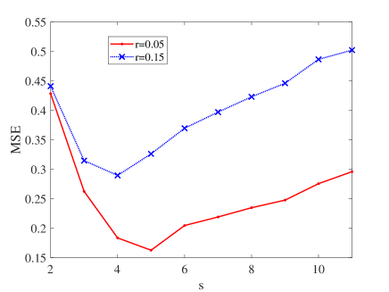
Figure 1: MSE of the solution yielded by GPSP with different $s$ (the data generated in the same way as in Section 5.1 with $(m,n,s^{*})=(500,1000,5),(\mu,\varpi)=(0.3,0.1)$ and $\Phi$ of type I)

The existing loss functions for the one-bit CS are mostly convex, including the one-sided $\ell_{2}$ loss [23, 46], the linear loss [31, 51], the one-sided $\ell_{1}$ loss [23, 46, 33], the pinball loss [21] and the logistic loss [16]. Among others, the one-sided $\ell_{1}$ loss is closely related to the hinge loss function in machine learning [11, 50], which was reported to have a superior performance to the one-sided $\ell_{2}$ loss (see [23]), and the pinball loss provides a bridge between the hinge loss and the linear loss. One can observe that these convex loss functions all impose a large penalty on the flipped samples, which inevitably imposes a negative effect on the solution quality of the model (3). In fact, for the pinball loss in [21], when the involved parameter $\tau$ is closer to $0$, the penalty degree on the flipped samples becomes smaller. This partly accounts for $\tau=-0.2$ instead of $\tau=-1$ used for numerical experiments there. Recently, Dai et al. [12] derived a one-sided zero-norm loss by maximizing a posteriori estimation of the true signal. This loss function and its lower semicontinuous (lsc) majorization proposed there impose a constant penalty for those flipped samples, but their combinatorial property brings much difficulty to the solution of the associated optimization models. Inspired by the superiority of the ramp loss in SVM [9, 22], in this work we are interested in a more general DC loss:

$$L_{\sigma}(z):=\sum_{i=1}^{m}\vartheta_{\!\sigma}(z_{i})\ \ {\rm with}\ \vartheta_{\!\sigma}(t):=\left\{\begin{array}[]{cl}\max(0,-t)&{\rm if}\ t\geq-\sigma,\\ \sigma&{\rm if}\ t<-\sigma,\end{array}\right.$$ (5)

where $\sigma\in(0,1]$ is a constant representing the penalty degree imposed on the flip outlier. Clearly, the DC function $\vartheta_{\!\sigma}$ imposes a small fixed penalty for those flip outliers.

Due to the nonconvexity of the zero-norm and the sphere constraint, some researchers are interested in the convex relaxation of (3) obtained by replacing the zero-norm by the $\ell_{1}$-norm and the unit sphere constraint by the unit ball constraint; see [51, 21, 24, 31]. However, as in the conventional CS, the $\ell_{1}$-norm convex relaxation not only has a weak sparsity-promoting ability but also leads to a biased solution; see the discussion in [14]. Motivated by this, many researchers resort to the nonconvex surrogate functions of the zero-norm, such as the minimax concave penalty (MCP) [53, 20], the sorted $\ell_{1}$ penalty [20], the logarithmic smoothing functions [40], the $\ell_{q}\,(0<\!q\!<1)$-norm [15], and the Schur-concave functions [32], and then develop algorithms for solving the associated nonconvex surrogate problems to achieve a better sparse solution. To the best of our knowledge, most of these algorithms are lack of convergence certificate. Although many nonconvex surrogates of the zero-norm are used for the one-bit CS, there is no work to investigate the equivalence between the surrogate problems and the model (3) in a global sense.

1.2 Main contributions

The nonsmooth DC loss $L_{\sigma}$ is desirable to ensure data fidelity and tolerate the existence of sign flips, but its nonsmoothness is inconvenient for the solution of the associated regularization model (3). With $0<\!\gamma<\!{\sigma}/{2}$ we construct a smooth approximation to it:

$$L_{\sigma,\gamma}(z):=\sum_{i=1}^{m}\vartheta_{\sigma,\gamma}(z_{i})\ \ {\rm with}\ \ \vartheta_{\sigma,\gamma}(t)\!:=\!\left\{\begin{array}[]{cl}0&{\rm if}\ t>0,\\ t^{2}/(2\gamma)&{\rm if}\ -\!\gamma<t\leq 0,\\ -t-\gamma/2&{\rm if}\ -\!\sigma\!+\!\gamma<t<-\gamma,\\ \!\sigma\!-\!\frac{\gamma}{2}\!-\!\frac{(t+\sigma+\gamma)^{2}}{4\gamma}&{\rm if}\ -\!(\sigma\!+\!\gamma)\leq t\leq\!\gamma\!-\!\sigma,\\ \!\sigma\!-\!{\gamma}/2&{\rm if}\ t<-(\sigma\!+\!\gamma).\end{array}\right.$$ (6)

Clearly, as the parameter $\gamma$ approaches to $0$, $\vartheta_{\!\sigma,\gamma}$ is closer to $\vartheta_{\!\sigma}$. As illustrated in Figure 2, the smooth function $\vartheta_{\!\sigma,\gamma}$ approximates $\vartheta_{\!\sigma}$ very well even with $\gamma=0.05$. Therefore, in this paper we are interested in the zero-norm regularized smooth DC loss model

$$\min_{x\in\mathbb{R}^{n}}F_{\sigma,\gamma}(x):=L_{\sigma,\gamma}(Ax)+\delta_{\mathcal{S}}(x)+\lambda\|x\|_{0},$$ (7)

where $\mathcal{S}$ denotes a unit sphere whose dimension is known from the context, and $\delta_{\mathcal{S}}$ means the indicator function of $\mathcal{S}$, i.e., $\delta_{\mathcal{S}}(x)=0$ if $x\in\mathcal{S}$ and otherwise $\delta_{\mathcal{S}}(x)=+\infty$.

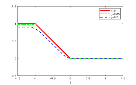
Figure 2: Approximation degree of $\vartheta_{\!\sigma,\gamma}$ with different $\gamma$ to $\vartheta_{\!\sigma}$ for $\sigma=1$

Let $\mathscr{L}$ denote the family of proper lsc convex functions $\phi\!:\mathbb{R}\to(-\infty,+\infty]$ satisfying

$${\rm int}({\rm dom}\,\phi)\supseteq[0,1],\ 1>t^{*}\!:=\mathop{\arg\min}_{0\leq t\leq 1}\phi(t),\ \phi(t^{*})=0\ \ {\rm and}\ \ \phi(1)=1.$$ (8)

With an arbitrary $\phi\in\!\mathscr{L}$, the model (7) is reformulated as a mathematical program with an equilibrium constraint (MPEC) in Section 3, and by studying its global exact penalty induced by the equilibrium constraint, we derive a family of equivalent surrogates

$$\mathop{\min}_{x\in\mathbb{R}^{n}}G_{\sigma,\gamma,\rho}(x):=L_{\sigma,\gamma}(Ax)+\delta_{\mathcal{S}}(x)+\lambda\rho\varphi_{\rho}(x),$$ (9)

in the sense that the problem (9) associated to every $\rho>\overline{\rho}$ has the same global optimal solution set as the problem (7) does. Here $\varphi_{\rho}(x)\!:=\!\|x\|_{1}-\!\frac{1}{\rho}\!\sum_{i=1}^{n}\psi^{*}(\rho|x_{i}|)$ with $\rho>0$ being the penalty parameter and $\psi^{*}$ being the conjugate function of $\psi$:

$$\psi^{*}(\omega):=\sup_{t\in\mathbb{R}}\big{\{}\omega t-\psi(t)\big{\}}\ \ {\rm for}\ \psi(t)\!:=\!\left\{\begin{array}[]{cl}\phi(t)&{\rm if}\ t\in[0,1],\\ +\infty&{\rm otherwise}.\end{array}\right.$$

This family of equivalent surrogates is illustrated to include the one associated to the MCP function (see [49, 53, 20]) and the SCAD function [14]. The SCAD function corresponds to $\phi(t)=\frac{a-1}{a+1}t^{2}+\frac{2}{a+1}t\ (a>1)$ for $t\in\mathbb{R}$, whose conjugate has the form

$$\psi^{*}(\omega)=\begin{cases}0&\omega\leq\frac{2}{a+1},\\ \frac{((a+1)\omega-2)^{2}}{4(a^{2}-1)}&\frac{2}{a+1}<\omega\leq\frac{2a}{a+1},\\ \omega-1&\omega>\frac{2a}{a+1},\end{cases}\quad{\rm for}\ \omega\in\mathbb{R}.$$ (10)

Figure 3 below shows that $G_{\sigma,\gamma,\rho}$ with $\psi^{*}$ in (10) approximates $F_{\sigma,\gamma}$ every well for $\rho\geq 2$, though the model (9) has the same global optimal solution set as the model (7) does only when $\rho$ is over the theoretical threshold $\overline{\rho}$. Unless otherwise stated, the function $G_{\sigma,\gamma,\rho}$ appearing in the rest of this paper always represents the one associated to $\psi^{*}$ in (10).

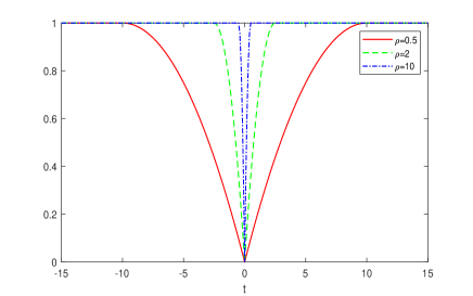
Figure 3: Approximation effect of $|t|-\rho^{-1}\psi^{*}(\rho|t|)$ with $\psi^{*}$ in (10) to ${\rm sign}(|t|)$

For the nonconvex nonsmooth optimization problems (7) and (9), we develop a proximal gradient (PG) method with extrapolation to solve them, establish the convergence of the whole iterate sequence generated, and analyze its local linear convergence rate under a mild condition. The main contributions of this paper can be summarized as follows:

• We introduce a smooth DC loss function well suited for the data with a high sign flip ratio, and propose the zero-norm regularized smooth DC loss model (7) which, unlike those models in [7, 12, 46, 52], does not require any priori information on the sparsity of the true signal and the number of sign flips. In particular, a family of equivalent nonconvex surrogates is derived for the model (7). We also introduce a class of $\tau$-stationary points for the model (7) and its equivalent surrogate (9) associated to $\psi^{*}$ in (10), which is stronger than the limiting critical points of the corresponding objective functions.

• By characterizing the closed form of the proximal operators of $\delta_{\mathcal{S}}(\cdot)+\lambda\|\cdot\|_{0}$ and $\delta_{\mathcal{S}}(\cdot)+\lambda\|\cdot\|_{1}$, we develop a proximal gradient (PG) algorithm with extrapolation for solving the problem (7) (PGe-znorm) and its surrogate (9) associated to $\psi^{*}$ in (10) (PGe-scad) and establish the convergence of the whole iterate sequences. Also, by analyzing the KL property of exponent $0$ of $F_{\sigma,\gamma}$ and $G_{\sigma,\gamma,\rho}$, the convergence is shown to have a linear rate under a mild condition. It is worth pointing out that to verify if a nonconvex and nonsmooth function has the KL property of exponent not more than $1/2$ is not an easy task because there is lack of a criterion for it.

• Numerical experiments indicate that the proposed models armed with the PGe-znorm and PGe-scad are robust to a large range of $\lambda$, and numerical comparisons with several state-of-art methods demonstrate that the proposed models are well suited for high noise and/or high sign flip ratio. The obtained solutions are remarkably superior to those yielded by other regularization models, and for the data with a high flip ratio they are also superior to those yielded by the models with the true sparsity as an input, in terms of MSE and Hamming error.

2 Notation and preliminaries

Throughout this paper, $\overline{\mathbb{R}}$ denotes the extended real number set $(-\infty,\infty]$, $I$ and $e$ denote an identity matrix and a vector of all ones, whose dimensions are known from the context; and $\{e^{1},\ldots,e^{n}\}$ denotes the orthonormal basis of $\mathbb{R}^{n}$. For a integer $k>0$, write $[k]:=\{1,2,\ldots,k\}$. For a vector $z\in\mathbb{R}^{n}$, $|z|_{\rm nz}$ denotes the smallest nonzero entry of the vector $|z|$, $z^{\downarrow}$ means the vector of the entries of $z$ arranged in a nonincreasing order, and $z^{s,\downarrow}$ means the vector $(z_{1}^{\downarrow},\ldots,z_{s}^{\downarrow})^{\mathbb{T}}$. For given index sets $I\subseteq[m]$ and $J\subseteq[n]$, $A_{I\!J}\in\mathbb{R}^{|I|\times|J|}$ denotes the submatrix of $A_{J}$ consisting of those rows $A_{i}$ with $i\in I$, and $A_{J}\in\mathbb{R}^{m\times|J|}$ denotes the submatrix of $A$ consisting of those columns $A_{j}$ with $j\in\!J$. For a proper $h\!:\mathbb{R}^{n}\to\overline{\mathbb{R}}$, ${\rm dom}\,h\!:=\!\{z\in\mathbb{R}^{n}\,|\,h(z)<+\infty\}$ denotes its effective domain, and for any given $-\infty<\eta_{1}<\eta_{2}<\infty$, $[\eta_{1}<h<\eta_{2}]$ represents the set $\{x\in\mathbb{R}^{n}\,|\,\eta_{1}<h(x)<\eta_{2}\}$. For any $\lambda>0,\rho>0,0<\gamma<\sigma/2$ and any $x\in\mathbb{R}^{n}$, write $\Gamma(x)\!:=\!\{i\in[m]\,|\,-\!\gamma\leq(Ax)_{i}\leq 0\}\cup\{i\in[m]\,|\,-\!\sigma\!-\!\gamma\leq(Ax)_{i}\leq\!\gamma\!-\!\sigma\}$ and define

$$f_{\sigma,\gamma}(x):=L_{\sigma,\gamma}(Ax),\ \ \Xi_{\sigma,\gamma}(x):=f_{\sigma,\gamma}(x)-\lambda{\textstyle\sum_{i=1}^{n}}\psi^{*}(\rho|x|_{i}),$$ (11)

$$g_{\lambda}(x):=\delta_{\mathcal{S}}(x)+\lambda\|x\|_{0}\ \ {\rm and}\ \ h_{\lambda,\rho}(x):=\delta_{\mathcal{S}}(x)+\lambda\rho\|x\|_{1}.$$ (12)

For a proper lsc $h\!:\mathbb{R}^{n}\to\overline{\mathbb{R}}$, the proximal mapping of $h$ associated to $\tau>0$ is defined as

$$\mathcal{P}_{\!\tau}h(x)\!:=\mathop{\arg\min}_{z\in\mathbb{R}^{n}}\big{\{}\frac{1}{2\tau}\|z-x\|^{2}+h(z)\big{\}}\quad\ \forall x\in\mathbb{R}^{n}.$$

When $h$ is convex, $\mathcal{P}_{\!\tau}h$ is a Lipschitz continuous mapping with modulus $1$. When $h$ is an indicator function of a closed set $C\subseteq\mathbb{R}^{n}$, $\mathcal{P}_{\!\tau}h$ is the projection mapping $\Pi_{C}$ onto $C$.

2.1 Proximal mappings of $g_{\lambda}$ and $h_{\lambda,\rho}$

To characterize the proximal mapping of the nonconvex nonsmooth function $g_{\lambda}$, we need the following lemma, whose proof is not included due to the simplicity.

Lemma 2.1

Fix any $z\in\mathbb{R}^{n}\backslash\{0\}$ and an integer $s\geq 1$. Consider the following problem

$$S^{*}(z):=\mathop{\arg\min}_{x\in\mathbb{R}^{n}}\Big{\{}\frac{1}{2}\|x-z\|^{2}\ \ {\rm s.t.}\ \ \|x\|=1,\|x\|_{0}=s\Big{\}}.$$ (13)

Then, $S^{*}(z)=\big{\{}\frac{P^{\mathbb{T}}(|z|^{s-1,\downarrow};|z|_{i};0)}{\|(|z|^{s-1,\downarrow};|z|_{i};0)\|}\,|\ i\in\{s,\ldots,n\}\ {\rm is\ such\ that}\ |z|_{i}=|z|_{s}^{\downarrow}\big{\}}$, where $P$ is an $n\times n$ signed permutation matrix such that $Pz=|z|^{\downarrow}$.

Proposition 2.1

Fix any $\lambda>0$ and $\tau>0$. For any $z\in\mathbb{R}^{n}$, by letting $P$ be an $n\times n$ signed permutation matrix such that $Pz=|z|^{\downarrow}$, it holds that $\mathcal{P}_{\!\tau}g_{\lambda}(z)=P^{\mathbb{T}}\mathcal{Q}_{\tau\lambda}(|z|^{\downarrow})$ with

$$\mathcal{Q}_{\nu}(y):=\mathop{\arg\min}_{x\in\mathbb{R}^{n}}\Big{\{}\frac{1}{2}\|x-y\|^{2}+\nu\|x\|_{0}\ \ {\rm s.t.}\ \|x\|=1\Big{\}}\quad\forall y\in\mathbb{R}^{n}.$$ (14)

For any $y\neq 0$ with $y_{1}\geq\cdots\geq y_{n}\geq 0$, by letting $\chi_{j}(y)\!:=\!\|y^{j,\downarrow}\|-\!\|y^{j-1,\downarrow}\|$ with $y^{0,\downarrow}=0$, $\mathcal{Q}_{\nu}(y)\!=\!\{\frac{y}{\|y\|}\}$ if $\nu\leq\!\chi_{n}(y)$; $\mathcal{Q}_{\nu}(y)\!=\!\big{\{}(\frac{y_{i}}{|y_{i}|},0,\ldots,0)^{\mathbb{T}}\,|\,i\in[n]\ {\rm is\ such\ that}\ y_{i}=y_{1}\big{\}}$ if $\nu\geq\!\chi_{1}(y)$; otherwise $\mathcal{Q}_{\nu}(y)\!:=\!\big{\{}(\frac{y^{l,\downarrow}}{\|y^{l,\downarrow}\|};0)\ |\ l\in[n]\ {\rm is\ such\ that}\ \nu\in(\chi_{l+1}(y),\chi_{l}(y)]\big{\}}$.

Proof: By the definition of $g_{\lambda}$, for any $z\in\mathbb{R}^{n}$, $\mathcal{P}_{\!\tau}g_{\lambda}(z)=\mathcal{Q}_{\tau\lambda}(z)$. Since for any $n\times n$ signed permutation matrix $Q$ and any $z\in\mathbb{R}^{n}$, $\|Qz\|=\|z\|$ and $\|Qz\|_{0}=\|z\|_{0}$, it is easy to verify that $\mathcal{Q}_{\nu}(z)=P^{\mathbb{T}}\mathcal{Q}_{\nu}(|z|^{\downarrow})$. The first part of the conclusions then follows. For the second part, we first argue that the following inequality relations hold:

$$\chi_{1}(y)\geq\chi_{2}(y)\geq\cdots\geq\chi_{n}(y).$$ (15)

Indeed, for each $j\in\{1,2,\ldots,n\!-\!1\}$, from the definition of $y^{j}$, it is immediate to have

$$\|y^{j}\|^{2}\!-\!\|y^{j-1}\|^{2}=y_{j}^{2}\geq y_{j+1}^{2}=\|y^{j+1}\|^{2}\!-\!\|y^{j}\|^{2}\ \ {\rm and}\ \ \|y^{j}\|\!+\!\|y^{j-1}\|\leq\|y^{j+1}\|\!+\!\|y^{j}\|.$$

Along with $\chi_{j}(y)=\frac{\|y^{j}\|^{2}-\|y^{j-1}\|^{2}}{\|y^{j}\|+\|y^{j-1}\|}$, we get $\chi_{j}(y)\geq\chi_{j+1}(y)$ and the relations in (15) hold. Let $\upsilon^{*}(y)$ denote the optimal value of (14). Then $\upsilon^{*}(y)=\min\{\overline{\chi}_{1}(y),\ldots,\overline{\chi}_{n}(y)\}$ with

$$\overline{\chi}_{s}(y):=\min_{x\in\mathbb{R}^{n}}\Big{\{}\frac{1}{2}\|x-y\|^{2}+\nu\|x\|_{0}\ \ {\rm s.t.}\ \ \|x\|_{0}=s,\|x\|=1\Big{\}}\ \ {\rm for}\ s=1,\ldots,n.$$ (16)

From Lemma 2.1, it follows that $\overline{\chi}_{s}(y)=\frac{1}{2}(1+\|y\|^{2}-2\|y^{s,\downarrow}\|)+\nu s$. Then,

$$\Delta\overline{\chi}_{s}(y):=\overline{\chi}_{s+1}(y)-\overline{\chi}_{s}(y)=\|y^{s,\downarrow}\|-\|y^{s+1,\downarrow}\|+\nu=-\chi_{s}(y)+\nu.$$

When $\nu\leq\chi_{n}(y)$, we have $\nu\leq\chi_{s}(y)$ for all $s=1,\ldots,n$. From the last equation, $\Delta\overline{\chi}_{s}(y)\leq 0$ for $s=1,\ldots,n-\!1$, which means that $\overline{\chi}_{1}(y)\geq\overline{\chi}_{2}(y)\geq\cdots\geq\overline{\chi}_{n}(y).$ Hence, $\upsilon^{*}(y)=\overline{\chi}_{n}(y)$, and $\mathcal{Q}_{\nu}(y)=\{\frac{y}{\|y\|}\}$ follows by Lemma 2.1. Using the similar arguments, we can obtain the rest of the conclusions. $\Box$

To characterize the proximal mapping of the nonconvex nonsmooth function $h_{\lambda,\rho}$, we need the following lemma, whose proof is omitted due to the simplicity.

Lemma 2.2

Let $\mathcal{S}_{+}:=\mathcal{S}\cap\mathbb{R}_{+}^{n}$. For any $z\in\!\mathbb{R}^{n}$, by letting $P$ be an $n\times n$ permutation matrix such that $Pz=z^{\downarrow}$, it holds that $\Pi_{\mathcal{S}_{+}}(z)=P^{\mathbb{T}}\Pi_{\mathcal{S}_{+}}(z^{\downarrow})$. Also, for any $y\!\in\mathbb{R}^{n}$ with $y_{1}\geq\cdots\geq y_{n}$, $\Pi_{\mathcal{S}_{+}}(y)=\big{\{}e_{i}\,|\,i\in[n]\ {\rm is\ such\ that}\ y_{i}=y_{1}\big{\}}$ if $y_{1}\leq 0$; $\Pi_{\mathcal{S}_{+}}(y)=\big{\{}\frac{y}{\|y\|}\big{\}}$ if $y_{n}\geq 0$, otherwise $\Pi_{\mathcal{S}_{+}}(y)=\big{\{}\frac{(y_{1},\ldots,y_{j},0,\ldots,0)^{\mathbb{T}}}{\|(y_{1},\ldots,y_{j},0,\ldots,0)^{\mathbb{T}}\|}\,|\,j\in[n\!-\!1]\ {\rm is\ such\ that}\ y_{j}>0\geq y_{j+1}\big{\}}$.

Proposition 2.2

Fix any $\lambda>0,\rho>0$ and $\tau>0$. For any $z\in\mathbb{R}^{n}$, by letting $P$ be an $n\times n$ signed permutation matrix with $Pz=|z|^{\downarrow}$, $\mathcal{P}_{\!\tau}h_{\lambda,\rho}(z)=P^{\mathbb{T}}\Pi_{\mathcal{S}_{+}}(|z|^{\downarrow}\!-\!\tau\lambda\rho e)$.

Proof: Fix any $\xi\in\mathbb{R}^{n}$ with $\xi_{1}\geq\xi_{2}\geq\cdots\geq\xi_{n}\geq 0$. Consider the following problem

$$\mathcal{P}_{\nu}(\xi):=\mathop{\arg\min}_{x\in\mathbb{R}^{n}}\Big{\{}\frac{1}{2}\big{\|}x-\xi\big{\|}^{2}+\nu\|x\|_{1}\ \ {\rm s.t.}\ \|x\|=1\Big{\}}$$ (17)

where $\nu>0$ is a regularization parameter. By the definition of $h_{\lambda,\rho}$, $\mathcal{P}_{\!\tau}h_{\lambda,\rho}(z)=\mathcal{P}_{\!\tau\lambda\rho}(z)$, so it suffices to argue that $\mathcal{P}_{\!\nu}(\xi)=\Pi_{\mathcal{S}_{+}}(\xi-\nu e)$. Indeed, if $x^{*}$ is a global optimal solution of (17), then $x^{*}\geq 0$ necessarily holds. If not, we will have $J:=\{j\,|\,x_{j}^{*}<0\}\neq\emptyset$. Let $\overline{J}=\{1,\ldots,n\}\backslash J$. Take $\widetilde{x}_{i}^{*}=x_{i}^{*}$ for each $i\in\overline{J}$ and $\widetilde{x}_{i}^{*}=-x_{i}^{*}$ for each $i\in J$. Clearly, $\widetilde{x}^{*}\geq 0$ and $\|\widetilde{x}^{*}\|=1$. However, it holds that $\frac{1}{2}\big{\|}\widetilde{x}^{*}-\xi\big{\|}^{2}+\nu\|\widetilde{x}^{*}\|_{1}\leq\frac{1}{2}\big{\|}x^{*}-\xi\big{\|}^{2}+\nu\|x^{*}\|_{1}$, which contradicts the fact that $x^{*}$ is a global optimal solution of (17). This implies that $\mathcal{P}_{\nu}(\xi)=\mathop{\arg\min}_{x\in\mathbb{R}^{n}}\big{\{}\frac{1}{2}\big{\|}x-\xi\big{\|}^{2}+\nu\langle e,x\rangle\ \ {\rm s.t.}\ x\geq 0,\|x\|=1\big{\}}.$ Consequently, $\mathcal{P}_{\nu}(\xi)=\Pi_{\mathcal{S}_{+}}(\xi-\nu e)$. The desired equality then follows. $\Box$

2.2 Generalized subdifferentials

Definition 2.1

(see [36, Definition 8.3]) Consider a function $h\!:\mathbb{R}^{n}\to\overline{\mathbb{R}}$ and a point $x\in{\rm dom}h$. The regular subdifferential of $h$ at $x$, denoted by $\widehat{\partial}h(x)$, is defined as

$$\widehat{\partial}h(x):=\bigg{\{}v\in\mathbb{R}^{n}\ \big{|}\ \liminf_{x^{\prime}\to x\atop x^{\prime}\neq x}\frac{h(x^{\prime})-h(x)-\langle v,x^{\prime}-x\rangle}{\|x^{\prime}-x\|}\geq 0\bigg{\}};$$

and the (limiting) subdifferential of $h$ at $x$, denoted by $\partial h(x)$, is defined as

$$\partial h(x):=\Big{\{}v\in\mathbb{R}^{n}\,|\,\exists\,x^{k}\to x\ {\rm with}\ h(x^{k})\to h(x)\ {\rm and}\ v^{k}\in\widehat{\partial}h(x^{k})\to v\ {\rm as}\ k\to\infty\Big{\}}.$$

Remark 2.1

(i) At each $x\in{\rm dom}h$, $\widehat{\partial}h(x)\subseteq\partial h(x)$, $\widehat{\partial}h(x)$ is always closed and convex, and $\partial h(x)$ is closed but generally nonconvex. When $h$ is convex, $\widehat{\partial}h(x)=\partial h(x)$, which is precisely the subdifferential of $h$ at $x$ in the sense of convex analysis.

(ii) Let $\{(x^{k},v^{k})\}_{k\in\mathbb{N}}$ be a sequence in the graph of $\partial h$ that converges to $(x,v)$ as $k\to\infty$. By invoking Definition 2.1, if $h(x^{k})\to h(x)$ as $k\to\infty$, then $v\in\partial h(x)$.

(iii) A point $\overline{x}$ at which $0\in\partial h(\overline{x})$ ($0\in\widehat{\partial}h(\overline{x})$) is called a limiting (regular) critical point of $h$. In the sequel, we denote by ${\rm crit}\,h$ the limiting critical point set of $h$.

When $h$ is an indicator function of a closed set $C$, the subdifferential of $h$ at $x\in C$ is the normal cone to $C$ at $x$, denoted by $\mathcal{N}_{C}(x)$. The following lemma characterizes the (regular) subdifferentials of $F_{\sigma,\gamma}$ and $G_{\sigma,\gamma,\rho}$ at any point of their domains.

Lemma 2.3

Fix any $\lambda>0,\rho>0$ and $0<\!\gamma<\!{\sigma}/{2}$. Consider any $x\in\mathcal{S}$. Then,

• $f_{\sigma,\gamma}$ is a smooth function whose gradient $\nabla\!f_{\sigma,\gamma}$ is Lipschitz continuous with the modulus $L_{\!f}\leq\frac{1}{\gamma}\|A\|^{2}$.

• $\widehat{\partial}F_{\sigma,\gamma}(x)=\partial F_{\sigma,\gamma}(x)=\nabla\!f_{\sigma,\gamma}(x)+\mathcal{N}_{\mathcal{S}}(x)+\lambda\partial\|x\|_{0}$.

• $\widehat{\partial}G_{\sigma,\gamma,\rho}(x)=\partial G_{\sigma,\gamma,\rho}(x)\!=\!\nabla\Xi_{\sigma,\gamma}(x)\!+\!\mathcal{N}_{\mathcal{S}}(x)+\lambda\rho\partial\|x\|_{1}$.

• When $|x|_{\rm nz}\geq\frac{2a}{\rho(a-1)}$, it holds that $\partial G_{\sigma,\gamma,\rho}(x)\subseteq\partial F_{\sigma,\gamma}(x)$.

Proof: (i) The result is immediate by the definition of $f_{\sigma,\gamma}$ and the expression of $L_{\sigma,\gamma}$.

(ii) From [42, Lemma 3.1-3.2 & 3.4], $\widehat{\partial}g_{\lambda}(x)=\partial g_{\lambda}(x)=\mathcal{N}_{\mathcal{S}}(x)+\lambda\partial\|x\|_{0}$. Together with part (i) and [36, Exercise 8.8], we obtain the desired result.

(iii) By the convexity and Lipschitz continuity of $\ell_{1}$-norm and [36, Exercise 10.10], it follows that $\partial h_{\lambda,\rho}(x)\!=\mathcal{N}_{\mathcal{S}}(x)+\lambda\rho\partial\|x\|_{1}$. Let $\theta_{\!\rho}(z)\!:=\!\rho^{-1}\sum_{i=1}^{n}\psi^{*}(\rho|z_{i}|)$ for $z\in\mathbb{R}^{n}$. Clearly, $\Xi_{\sigma,\gamma}=f_{\sigma,\gamma}-\lambda\rho\theta_{\!\rho}$. By the expression of $\psi^{*}$ in (10), it is easy to verify that $\theta_{\!\rho}$ is smooth and $\nabla\theta_{\!\rho}$ is Lipschitz continuous with modulus $\rho\max(\frac{a+1}{2},\frac{a+1}{2(a-1)})$. Hence, $\Xi_{\sigma,\gamma}$ is a smooth function whose gradient is Lipschitz continuous. Together with [36, Exercise 8.8] and $G_{\sigma,\gamma,\rho}=\Xi_{\sigma,\gamma}+h_{\lambda,\rho}$, we obtain the desired equalities.

(iv) Let $\theta_{\!\rho}$ be the function defined as above. After an elementary calculation, we have

$$\nabla\theta_{\!\rho}(x)\!=\big{(}(\psi^{*})^{\prime}(\rho|x_{1}|){\rm sign}(x_{1}),\ldots,(\psi^{*})^{\prime}(\rho|x_{n}|){\rm sign}(x_{n})\big{)}^{\mathbb{T}}.$$

Along with $|x|_{\rm nz}\geq\frac{2a}{\rho(a-1)}$ and the expression of $\psi^{*}$ in (10), we have $\nabla\theta_{\!\rho}(x)={\rm sign}(x)$ and $\partial\|x\|_{1}\!-\!\nabla\theta_{\!\rho}(x)\subseteq\rho\partial\|x\|_{0}$. By part (iii), $\nabla\Xi_{\sigma,\gamma}(x)=\nabla\!f_{\sigma,\gamma}(x)-\lambda\rho\nabla\theta_{\!\rho}(x)$. Comparing $\partial G_{\sigma,\gamma,\rho}(x)$ in part (iii) with $\partial F_{\sigma,\gamma}(x)$ in part (ii) yields that $\partial G_{\sigma,\gamma,\rho}(x)\subseteq\partial F_{\sigma,\gamma}(x)$. $\Box$

2.3 Stationary points

Lemma 2.3 shows that for the functions $F_{\sigma,\gamma}$ and $G_{\sigma,\gamma,\rho}$ the set of their regular critical points coincides with that of their limiting critical points, so we call the critical point of $F_{\sigma,\gamma}$ a stationary point of (7), and the critical point of $G_{\sigma,\gamma,\rho}$ a stationary point of (9). Motivated by the work [4], we introduce a class of $\tau$-stationary points for them.

Definition 2.2

Let $\tau>0$. A vector $x\in\mathbb{R}^{n}$ is called a $\tau$-stationary point of (7) if $x\in\mathcal{P}_{\!\tau}g_{\lambda}(x\!-\!\tau\nabla\!f_{\sigma,\gamma}(x))$, and is called a $\tau$-stationary point of (9) if $x\in\mathcal{P}_{\!\tau}h_{\lambda,\rho}(x\!-\!\tau\nabla\Xi_{\sigma,\gamma}(x))$.

In the sequel, we denote by $S_{\tau,g_{\lambda}}$ and $S_{\tau,h_{\lambda,\rho}}$ the $\tau$-stationary point set of (7) and (9), respectively. By Proposition 2.1 and 2.2, we have the following result for them.

Lemma 2.4

Fix any $\tau>0,\lambda>0,\rho>0$ and $0<\!\gamma<\!{\sigma}/{2}$. Then, $S_{\tau,g_{\lambda}}\subseteq{\rm crit}F_{\sigma,\gamma}$ and $S_{\tau,h_{\lambda,\rho}}\subseteq{\rm crit}G_{\sigma,\gamma,\rho}$.

Proof: Pick any $\overline{x}\in\!S_{\tau,g_{\lambda}}$. Then $\overline{x}=\mathcal{P}_{\!\tau}g_{\lambda}(\overline{x}\!-\!\tau\nabla\!f_{\sigma,\gamma}(\overline{x}))$. By Proposition 2.1, for each $i\in{\rm supp}(\overline{x})$, $\overline{x}_{i}=\alpha^{-1}[\overline{x}_{i}\!-\!\tau(\nabla\!f_{\sigma,\gamma}(\overline{x}))_{i}]$ for some $\alpha\!>0$ (depending on $\overline{x}$). Then, for each $i\in{\rm supp}(\overline{x})$, it holds that $(\nabla\!f_{\sigma,\gamma}(\overline{x}))_{i}+\tau^{-1}(\alpha\!-\!1)\overline{x}_{i}=0$. Recall that

$$\mathcal{N}_{\mathcal{S}}(\overline{x})=\big{\{}\beta\overline{x}\,|\,\beta\in\mathbb{R}\big{\}}\ \ {\rm and}\ \ \partial\|\overline{x}\|_{0}=\big{\{}v\in\mathbb{R}^{n}\,|\,v_{i}=0\ {\rm for}\ i\in{\rm supp}(\overline{x})\big{\}}.$$ (18)

We have $0\in\nabla\!f_{\sigma,\gamma}(\overline{x})+\mathcal{N}_{\mathcal{S}}(\overline{x})+\lambda\partial\|\overline{x}\|_{0}$, and hence $\overline{x}\in{\rm crit}F_{\sigma,\gamma}$ by Lemma 2.3 (ii).

Pick any $\overline{x}\in\!S_{\tau,h_{\lambda,\rho}}$. Write $\overline{u}=\overline{x}\!-\!\tau\nabla\Xi_{\sigma,\gamma}(\overline{x})$. Then, we have $\overline{x}=\mathcal{P}_{\!\tau}h_{\lambda,\rho}(\overline{u})$. Let $J\!:=\{i\in[n]\,|\,|\overline{u}_{i}|>\tau\lambda\rho\}$ and $\overline{J}=[n]\backslash J$. For each $i\in\overline{J}$, $|\nabla\Xi_{\sigma,\gamma}(\overline{x})-\tau^{-1}\overline{x}_{i}|\leq\lambda\rho$. Since the subdifferential of the function $t\mapsto|t|$ at $0$ is $[-1,1]$, it holds that

$$0\in[\nabla\Xi_{\sigma,\gamma}(\overline{x})]_{\overline{J}}-\tau^{-1}\overline{x}_{\overline{J}}+\lambda\rho\partial\|\overline{x}_{\overline{J}}\|_{1}.$$

By Proposition 2.2, we have $\overline{x}_{J}=\frac{\overline{u}_{J}-\tau\lambda\rho{\rm sign}(\overline{u}_{J})}{\|\overline{u}_{J}-\tau\lambda\rho{\rm sign}(\overline{u}_{J})\|}.$ Together with ${\rm sign}(\overline{u}_{J})={\rm sign}(\overline{x}_{J})$,

$$(\nabla\Xi_{\sigma,\gamma}(\overline{x}))_{J}+\tau^{-1}(\|\overline{u}_{J}\!-\!\tau\lambda\rho{\rm sign}(\overline{u}_{J})\|\!-\!1)\overline{x}_{J}+\lambda\rho{\rm sign}(\overline{x}_{J})=0.$$

By the expression of $\mathcal{N}_{\mathcal{S}}(\overline{x})$ in (18), from the last two equations it follows that

$$0\in\nabla\Xi_{\sigma,\gamma}(\overline{x})+\mathcal{N}_{\mathcal{S}}(\overline{x})+\lambda\rho\partial\|\overline{x}\|_{1}.$$

By Lemma 2.3 (iii), this shows that $\overline{x}\in{\rm crit}G_{\sigma,\gamma,\rho}$. The proof is completed. $\Box$

Note that if $\overline{x}$ is a stationary point of (7), then for $i\notin{\rm supp}(\overline{x})$, $[\mathcal{P}_{\!\tau}g_{\lambda}(\overline{x}\!-\!\tau\nabla\!f_{\sigma,\gamma}(\overline{x}))]_{i}$ does not necessarily equal $0$. A similar case also occurs for the stationary point of (9). This means that the two inclusions in Lemma 2.4 are generally strict. By combining Lemma 2.4 with [36, Theorem 10.1], it is immediate to obtain the following conclusion.

Corollary 2.1

Fix any $\tau>0$. For the problems (7) and (9), their local optimal solution is necessarily is a stationary point, and consequently a $\tau$-stationary point.

2.4 Kurdyka-Łöjasiewicz property

Definition 2.3

(see [2]) A proper lsc function $h\!:\mathbb{R}^{n}\to\overline{\mathbb{R}}$ is said to have the KL property at $\overline{x}\in{\rm dom}\,\partial h$ if there exist $\eta\in(0,+\infty]$, a neighborhood $\mathcal{U}$ of $\overline{x}$, and a continuous concave function $\varphi\!:[0,\eta)\to\mathbb{R}_{+}$ that is continuously differentiable on $(0,\eta)$ with $\varphi^{\prime}(s)>0$ for all $s\in(0,\eta)$ and $\varphi(0)=0$, such that for all $x\in\mathcal{U}\cap\big{[}h(\overline{x})<h<h(\overline{x})+\eta\big{]}$,

$$\varphi^{\prime}(h(x)-h(\overline{x})){\rm dist}(0,\partial h(x))\geq 1.$$

If $\varphi$ can be chosen as $\varphi(t)=ct^{1-\theta}$ with $\theta\in[0,1)$ for some $c>0$, then $h$ is said to have the KL property of exponent $\theta$ at $\overline{x}$. If $h$ has the KL property (of exponent $\theta$) at each point of ${\rm dom}\,\partial h$, then it is called a KL function (of exponent $\theta$).

Remark 2.2

(a) As discussed thoroughly in [2, Section 4], there are a large number of nonconvex nonsmooth functions are the KL functions, which include real semi-algebraic functions and those functions definable in an o-minimal structure.

(b) From [2, Lemma 2.1], a proper lsc function has the KL property of exponent $\theta=0$ at any noncritical point. Thus, to prove that a proper lsc $h\!:\mathbb{R}^{n}\to\overline{\mathbb{R}}$ is a KL function (of exponent $\theta$), it suffices to achieve its KL property (of exponent $\theta$) at critical points. On the calculation of KL exponent, please refer to the recent works [34, 48].

3 Equivalent surrogates of the model (7)

Pick any $\phi\in\!\mathscr{L}$. By invoking equation (8), it is immediate to verify that for any $x\in\mathbb{R}^{n}$,

$$\|x\|_{0}=\min_{w\in[0,e]}\Big{\{}\textstyle{\sum_{i=1}^{n}}\phi(w_{i})\ \ {\rm s.t.}\ \langle e-\!w,|x|\rangle=0\Big{\}}.$$

This means that the zero-norm regularized problem (7) can be reformulated as

$$\min_{x\in\mathcal{S},w\in[0,e]}\Big{\{}f_{\sigma,\gamma}(x)+\lambda\textstyle{\sum_{i=1}^{n}}\phi(w_{i})\quad\mbox{s.t.}\ \ \langle e-w,|x|\rangle=0\Big{\}}$$ (19)

in the following sense: if $x^{*}$ is globally optimal to the problem (7), then $(x^{*}\!,{\rm sign}(|x^{*}|))$ is a global optimal solution of the problem (19), and conversely, if $(x^{*},w^{*})$ is a global optimal solution of (19), then $x^{*}$ is globally optimal to (7). The problem (19) is a mathematical program with an equilibrium constraint $e\!-\!w\geq 0,|x|\geq 0,\langle e-w,|x|\rangle=0$. In this section, we shall show that the penalty problem induced by this equilibrium constraint, i.e.,

$$\min_{x\in\mathcal{S},w\in[0,e]}\Big{\{}f_{\sigma,\gamma}(x)+\lambda\textstyle{\sum_{i=1}^{n}}\phi(w_{i})+\rho\lambda\langle e-w,|x|\rangle\Big{\}}$$ (20)

is a global exact penalty of (19) and from this global exact penalty achieve the equivalent surrogate in (9), where $\rho>0$ is the penalty parameter. For each $s\in[n]$, write

$$\Omega_{s}:=\mathcal{S}\cap\mathcal{R}_{s}\ \ {\rm with}\ \ \mathcal{R}_{s}:=\{x\in\mathbb{R}^{n}\,|\,\|x\|_{0}\leq s\}.$$

To get the conclusion of this section, we need the following global error bound result.

Lemma 3.1

For each $s\in\{1,2,\ldots,n\}$, there exists $\kappa_{s}>0$ such that for all $x\in\mathcal{S}$,

$${\rm dist}(x,\Omega_{s})\leq\kappa_{s}\big{[}\|x\|_{1}-\|x\|_{(s)}\big{]},$$

where $\|x\|_{(s)}$ denotes the sum of the first $s$ largest entries of the vector $x\in\mathbb{R}^{n}$.

Proof: Fix any $s\in\{1,2,\ldots,n\}$. We first argue that the following multifunction

$$\Upsilon_{\!s}(\tau):=\big{\{}x\in\mathcal{S}\,|\,\|x\|_{1}-\|x\|_{(s)}=\tau\big{\}}\ \ {\rm for}\ \tau\in\mathbb{R}$$

is calm at $0$ for every $x\in\Upsilon_{\!s}(0)$. Pick any $\widehat{x}\in\Upsilon_{\!s}(0)$. By [39, Theorem 3.1], the calmness of $\Upsilon_{\!s}$ at $0$ for $\widehat{x}$ is equivalent to the existence of $\delta>0$ and $\kappa>0$ such that

$${\rm dist}(x,\Omega_{s})\leq\kappa\big{[}{\rm dist}(x,\mathcal{S})+{\rm dist}(x,\mathcal{R}_{s})\big{]}\ \ {\rm for\ all}\ x\in\mathbb{B}(\widehat{x},\delta).$$ (21)

Since $\|\widehat{x}\|=1$, there exists $\varepsilon\in(0,1/2)$ such that for all $x\in\mathbb{B}(\widehat{x},\varepsilon)$, $x\neq 0$. Fix any $x\in\mathbb{B}(\widehat{x},{\varepsilon}/{2})$. Clearly, $\|x\|\geq\|\widehat{x}\|-{\varepsilon}/{2}\geq{3}/{4}$. This means that $\|x\|_{\infty}\!\geq\frac{3}{4\sqrt{n}}$. Pick any $x^{*}\in\Pi_{\mathcal{R}_{s}}(x)$. Clearly, $\|x^{*}\|_{\infty}=\|x\|_{\infty}\geq\frac{3}{4\sqrt{n}}$ and $\frac{x^{*}}{\|x^{*}\|}\in\Omega_{s}$. Then, with $\overline{x}=\frac{x}{\|x\|}$,

$${\rm dist}(x,\Omega_{s}) \leq\|x-x^{*}\!/{\|x^{*}\|}\|\leq\|x-\overline{x}\|+\|\overline{x}-x^{*}\!/{\|x^{*}\|}\|$$

$$\leq\|x-\overline{x}\|+\frac{\|(x-x^{*})\|x\|+x(\|x^{*}\|-\|x\|)\|}{\|x\|\|x^{*}\|}$$

$$\leq\|x-\overline{x}\|+(2/\|x^{*}\|)\|x-x^{*}\|\leq{\rm dist}(x,\mathcal{S})+3\sqrt{n}{\rm dist}(x,\mathcal{R}_{s}).$$

This shows that the inequality (21) holds for $\delta=\varepsilon/2$ and $\kappa=3\sqrt{n}$. Consequently, the mapping $\Upsilon_{\!s}$ is calm at $0$ for every $x\in\Upsilon_{\!s}(0)$. Now by invoking [39, Theorem 3.3] and the compactness of $\mathcal{S}$, we obtain the desired result. The proof is completed. $\Box$

Now we are ready to show that the problem (20) is a global exact penalty of (19).

Proposition 3.1

Let $\overline{\rho}:=\frac{\kappa\phi_{-}^{\prime}(1)(1-t^{*})\alpha_{\!f}}{\lambda(1-t_{0})}$ where $t_{0}\in[0,1)$ is such that $\frac{1}{1-t^{*}}\in\partial\phi(t_{0})$, $\phi_{-}^{\prime}(1)$ is the left derivative of $\phi$ at $1$, $\alpha_{\!f}$ is the Lipschitz constant of $f_{\sigma,\gamma}$ on $\mathcal{S}$, and $\kappa=\max_{1\leq s\leq n}\kappa_{s}$ with $\kappa_{s}$ given by Lemma 3.1. Then, for any $(x,w)\in\mathcal{S}\times[0,e]$,

$$\big{[}f_{\sigma,\gamma}(x)+\lambda{\textstyle\sum_{i=1}^{n}}\phi(w_{i})\big{]}-\big{[}f_{\sigma,\gamma}(x^{*})+\lambda{\textstyle\sum_{i=1}^{n}}\phi(w_{i}^{*})\big{]}+\overline{\rho}\lambda\langle e\!-\!w,|x|\rangle\geq 0,$$ (22)

where $(x^{*},w^{*})$ is an arbitrary global optimal solution of (19), and consequently the problem (20) associated to each $\rho>\overline{\rho}$ has the same global optimal solution set as (19) does.

Proof: By Lemma 3.1 and $\kappa=\max_{1\leq s\leq n}\kappa_{s}$, for each $s\in\{1,2,\ldots,n\}$ and any $z\in\mathcal{S}$,

$${\rm dist}(z,\mathcal{S}\cap\mathcal{R}_{s})\leq\kappa\big{[}\|z\|_{1}-\|z\|_{(k)}\big{]}.$$ (23)

Fix any $(x,w)\in\mathcal{S}\times[0,e]$. Let $J=\big{\{}j\in[n]\,|\ \overline{\rho}|x|_{j}^{\downarrow}>\phi_{-}^{\prime}(1)\big{\}}$ and $r=|J|$. By invoking (23) for $s=r$ with $z=x$, there exists $x^{\overline{\rho}}\in\mathcal{S}\cap\mathcal{R}_{r}$ such that

$$\|x-x^{\overline{\rho}}\|\leq\kappa\big{[}\|x\|_{1}-\|x\|_{(r)}\big{]}=\kappa{\textstyle\sum_{j=r+1}^{n}}|x|_{j}^{\downarrow}.$$ (24)

Let $J_{1}=\!\big{\{}j\in[n]\,|\,\frac{1}{1-t^{*}}\!\leq\!\overline{\rho}|x|_{j}^{\downarrow}\leq\phi_{-}^{\prime}(1)\big{\}}$ and $J_{2}=\!\big{\{}j\in[n]\,|\,0\!\leq\!\overline{\rho}|x|_{j}^{\downarrow}<\frac{1}{1-t^{*}}\big{\}}$. Note that

$${\textstyle\sum_{i=1}^{n}}\phi(w_{i})+\overline{\rho}\big{(}\|x\|_{1}\!-\langle w,|x|\rangle\big{)}\geq{\textstyle\sum_{i=1}^{n}}\min_{t\in[0,1]}\big{\{}\phi(t)+\overline{\rho}|x|_{i}^{\downarrow}(1-t)\big{\}}.$$

By invoking [35, Lemma 1] with $\omega=|x|_{j}^{\downarrow}$ for each $j$, it immediately follows that

$${\textstyle\sum_{i=1}^{n}}\phi(w_{i})+\overline{\rho}\big{(}\|x\|_{1}\!-\langle w,x\rangle\big{)}\geq\|x^{\overline{\rho}}\|_{0}+\frac{\overline{\rho}(1\!-\!t_{0})}{\phi_{-}^{\prime}(1)(1\!-t^{*})}\sum_{j\in J_{1}}\,|x|_{j}^{\downarrow}+\overline{\rho}(1\!-\!t_{0})\sum_{j\in J_{2}}\,|x|_{j}^{\downarrow}.$$

Notice that $1=\phi(1)=\phi(1)-\phi(t^{*})\leq\phi_{-}^{\prime}(1)(1-t^{*})$. From the last inequality, we have

$${\textstyle\sum_{i=1}^{n}}\phi(w_{i})+\overline{\rho}\big{(}\|x\|_{1}\!-\langle w,x\rangle\big{)}\geq\|x^{\overline{\rho}}\|_{0}+\frac{\overline{\rho}(1-t_{0})}{\phi_{-}^{\prime}(1)(1\!-t^{*})}\sum_{j\in J_{1}\cup J_{2}}|x|_{j}^{\downarrow}$$

$$=\|x^{\overline{\rho}}\|_{0}+\frac{\overline{\rho}(1-t_{0})}{\phi_{-}^{\prime}(1)(1\!-t^{*})}\sum_{j=r+1}^{n}|x|_{j}^{\downarrow}\geq\|x^{\overline{\rho}}\|_{0}+\alpha_{\!f}\lambda^{-1}\|x-x^{\overline{\rho}}\|\qquad$$ (25)

where the last inequality is due to (24) and the definition of $\overline{\rho}$. Since $x\in\mathcal{S}$ and $x^{\overline{\rho}}\in\mathcal{S}$, we have $f_{\sigma,\gamma}(x^{\overline{\rho}})-f_{\sigma,\gamma}(x)\leq\alpha_{\!f}\|x-x^{\overline{\rho}}\|$. Together with the last inequality,

$${\textstyle\sum_{i=1}^{n}}\phi(w_{i})+\overline{\rho}\big{(}\|x\|_{1}\!-\langle w,x\rangle\big{)}\geq\|x^{\overline{\rho}}\|_{0}+\lambda^{-1}\big{[}f_{\sigma,\gamma}(x^{\overline{\rho}})-f_{\sigma,\gamma}(x)\big{]}.$$ (26)

Now take $w_{i}^{\overline{\rho}}=1$ for $i\in{\rm supp}(x^{\overline{\rho}})$ and $w_{i}^{\overline{\rho}}=0$ for $i\notin{\rm supp}(x^{\overline{\rho}})$. Clearly, $(x^{\overline{\rho}},w^{\overline{\rho}})$ is a feasible point of the MPEC (19) with $\sum_{i=1}^{n}\phi(w_{i}^{\overline{\rho}})=\|x^{\overline{\rho}}\|_{0}$. Then, it holds that

$$f_{\sigma,\gamma}(x^{\overline{\rho}})+\lambda\|x^{\overline{\rho}}\|_{0}\geq f_{\sigma,\gamma}(x^{*})+\lambda{\textstyle\sum_{i=1}^{n}}\phi(w_{i}^{*}).$$

Together with (26), we obtain the inequality (22). Notice that $\langle e\!-\!w^{*},|x^{*}|\rangle=0$. The inequality (22) implies that every global optimal solution of (19) is globally optimal to the problem (20) associated to every $\rho>\overline{\rho}$. Conversely, by fixing any $\rho>\overline{\rho}$ and letting $(\overline{x}^{\rho},\overline{w}^{\rho})$ be a global optimal solution of the problem (20) associated to $\rho$, it holds that

$$f_{\sigma,\gamma}(\overline{x}^{\rho})+\lambda\textstyle{\sum_{i=1}^{n}}\phi(\overline{w}_{i}^{\rho})+\rho\lambda\langle e-\overline{w}^{\rho},|\overline{x}^{\rho}|\rangle$$

$$\leq f_{\sigma,\gamma}(x^{*})+\lambda\textstyle{\sum_{i=1}^{n}}\phi(w_{i}^{*})=f_{\sigma,\gamma}(x^{*})+\lambda\textstyle{\sum_{i=1}^{n}}\phi(w_{i}^{*})+\frac{\rho+\overline{\rho}}{2}\lambda\langle e-\overline{w}^{\rho},|\overline{x}^{\rho}|\rangle$$

$$\leq f_{\sigma,\gamma}(\overline{x}^{\rho})+\lambda\textstyle{\sum_{i=1}^{n}}\phi(\overline{w}_{i}^{\rho})+\frac{\rho+\overline{\rho}}{2}\lambda\langle e-\overline{w}^{\rho},|\overline{x}^{\rho}|\rangle,$$

which implies that $\frac{\rho-\overline{\rho}}{2}\lambda\langle e-\overline{w}^{\rho},|\overline{x}^{\rho}|\rangle\leq 0$. Since $\rho>\overline{\rho}$ and $\langle e-\overline{w}^{\rho},|\overline{x}^{\rho}|\rangle\geq 0$, we obtain $\langle e-\overline{w}^{\rho},|\overline{x}^{\rho}|\rangle=0$. Together with the last inequality, it follows that $(\overline{x}^{\rho},\overline{w}^{\rho})$ is a global optimal solution of (19). The second part then follows. $\Box$

By the definition of $\psi$, the penalty problem (20) can be rewritten in a compact form

$$\min_{x\in\mathcal{S},w\in\mathbb{R}^{n}}\big{\{}f_{\sigma,\gamma}(x)+\lambda\textstyle{\sum_{i=1}^{n}}\psi(w_{i})+\rho\lambda\langle e-w,|x|\rangle\big{\}},$$

which, by the definition of the conjugate function $\psi^{*}$, can be simplified to be (9). Then, Proposition 3.1 implies that the problem (9) associated to every $\phi\in\!\mathscr{L}$ and $\rho>\overline{\rho}$ is an equivalent surrogate of the problem (7). For a specific $\phi$, since $t^{*},t_{0}$ and $\phi_{-}^{\prime}(1)$ are known, the threshold $\overline{\rho}$ is also known by Lemma 3.1 though $\kappa=3\sqrt{n}$ is a rough estimate.

When $\phi$ is the one in Section 1.2, it is easy to verify that $\lambda\rho\varphi_{\rho}$ with $\lambda=\frac{(a+1)\nu^{2}}{2}$ and $\rho=\frac{2}{(a+1)\nu}$ is exactly the SCAD function $x\mapsto\sum_{i=1}^{n}\rho_{\nu}(x_{i})$ proposed in [14]. Since $t^{*}=0,t_{0}=1/2$ and $\phi_{-}^{\prime}(1)=\frac{2a}{a+1}$ for this $\phi$, the SCAD function with $\nu<\frac{2}{(a+1)\overline{\rho}}$ is an equivalent surrogate of (7). When $\phi(t)=\frac{a^{2}}{4}t^{2}-\frac{a^{2}}{2}t+at+\frac{(a-2)^{2}}{4}\ (a>2)$ for $t\in\mathbb{R}$,

$$\psi^{*}(\omega)=\left\{\begin{array}[]{cl}-\frac{(a-2)^{2}}{4}&\textrm{if}\ \omega\leq a-a^{2}/2,\\ \frac{1}{a^{2}}(\frac{a(a-2)}{2}+\omega)^{2}-\frac{(a-2)^{2}}{4}&\textrm{if}\ a-a^{2}/2<\omega\leq a,\\ \omega-1&\textrm{if}\ \omega>a.\end{array}\right.$$

It is not hard to verify that the function $\lambda\rho\varphi_{\rho}$ with $\lambda={a\nu^{2}}/{2}$ and $\rho={1}/{\nu}$ is exactly the one $x\mapsto\sum_{i=1}^{n}g_{\nu,b}(x_{i})$ with $b=a$ used in [20, Section 3.3]. Since $t^{*}=\frac{a-2}{a},t_{0}=\frac{a-1}{a}$ and $\phi_{-}^{\prime}(1)=a$ for this $\phi$, the MCP function used in [20] with $\nu<1/{\overline{\rho}}$ and $b=a$ is also an equivalent surrogate of the problem (7).

4 PG method with extrapolation

4.1 PG with extrapolation for solving (7)

Recall that $f_{\sigma,\gamma}$ is a smooth function whose gradient $\nabla\!f_{\sigma,\gamma}$ is Lipschitz continuous with modulus $L_{\!f}\leq\gamma^{-1}\|A\|^{2}$. While by Proposition 2.1 the proximal mapping of $g_{\lambda}$ has a closed form. This inspires us to apply the PG method with extrapolation to solving (7).

Algorithm 1 (PGe-znorm for solving the problem (7))

Initialization: Choose $\varsigma\in(0,1),0<\tau<(1\!-\!\varsigma)L_{\!f}^{-1},0<\beta_{\rm max}\leq\frac{\sqrt{\varsigma(\tau^{-1}-L_{\!f})\tau^{-1}}}{2(\tau^{-1}+L_{\!f})}$ and an initial point $x^{0}\in\mathcal{S}$. Set $x^{-1}=x^{0}$ and $k:=0$.

while the termination condition is not satisfied do

• Let $\widetilde{x}^{k}=x^{k}+\beta_{k}(x^{k}-x^{k-1})$. Compute $x^{k+1}\in\mathcal{P}_{\!\tau}g_{\lambda}(\widetilde{x}^{k}\!-\!\tau\nabla\!f_{\sigma,\gamma}(\widetilde{x}^{k}))$.

• Choose $\beta_{k+1}\in[0,\beta_{\rm max}]$. Let $k\leftarrow k+1$ and go to Step 1.

end (while)

Remark 4.1

The main computation work of Algorithm 1 in each iteration is to seek

$$x^{k+1}\in\mathop{\arg\min}_{x\in\mathbb{R}^{n}}\Big{\{}\langle\nabla\!f_{\sigma,\gamma}(\widetilde{x}^{k}),x-\widetilde{x}^{k}\rangle+\frac{1}{2\tau}\|x-\widetilde{x}^{k}\|^{2}+g_{\lambda}(x)\Big{\}}.$$ (27)

By Proposition 2.1, to achieve a global optimal solution of the nonconvex problem (27) requires about $2mn$ flops. Owing to the good performance of the Nesterov’s acceleration strategy [37, 38], one can use this strategy to choose the extrapolation parameter $\beta_{k}$, i.e.,

$$\beta_{k}=\frac{t_{k-1}-1}{t_{k}}\ \ {\rm with}\ t_{k+1}=\frac{1}{2}\big{(}1+\!\sqrt{1+4t_{k}^{2}}\big{)}\ \ {\rm for}\ t_{-1}=t_{0}=1.$$ (28)

In Algorithm 1, an upper bound $\beta_{\rm max}$ is imposed on $\beta_{k}$ just for the convergence analysis. It is easy to check that as $\varsigma$ approaches to $1$, say $\varsigma=0.999$, $\beta_{\rm max}$ can take $0.235$.

The PG method with extrapolation, first proposed in [37] and extended to a general composite setting in [3], is a popular first-order one for solving nonconvex nonsmooth composite optimization problems such as (7) and (9). In the past several years, the PGe and its variants have received extensive attentions (see, e.g., [17, 27, 41, 29, 28, 45, 47]). Due to the nonconvexity of the sphere constraint and the zero-norm, the results obtained in [17, 41, 29] are not applicable to (7). Although Algorithm 1 is a special case of those studied in [27, 45, 47], the convergence results of [27, 47] are obtained for the objective value sequence and the convergence result of [45] on the iterate sequence requires a strong restriction on $\beta_{k}$, i.e., it is such that the objective value sequence is nonincreasing.

Next we provide the proof for the convergence and local convergence rate of the iterate sequence yielded by Algorithm 1. For any $\tau>0$ and $\varsigma\in(0,1)$, we define the function

$$H_{\tau,\varsigma}(x,u):=F_{\sigma,\gamma}(x)+\frac{\varsigma}{4\tau}\|x-u\|^{2}\quad\ \forall(x,u)\in\mathbb{R}^{n}\times\mathbb{R}^{n}.$$ (29)

The following lemma summarizes the properties of $H_{\tau,\zeta}$ on the sequence $\{x^{k}\}_{k\in\mathbb{N}}$.

Lemma 4.1

Let $\{x^{k}\}_{k\in\mathbb{N}}$ be the sequence generated by Algorithm 1. Then,

• for each $k\in\mathbb{N}$, $H_{\tau,\varsigma}(x^{k+1},x^{k})\leq H_{\tau,\varsigma}(x^{k},x^{k-1})-\frac{\varsigma(\tau^{-1}-L_{\!f})}{2}\|x^{k+1}\!-\!x^{k}\|^{2}.$

• The sequence $\{H_{\tau,\varsigma}(x^{k},x^{k-1})\}_{k\in\mathbb{N}}$ is convergent and $\sum_{k=1}^{\infty}\|x^{k+1}\!-\!x^{k}\|^{2}<\infty$.

• For each $k\in\mathbb{N}$, there exists $w^{k}\in\partial H_{\tau,\varsigma}(x^{k},x^{k-1})$ with $\|w^{k+1}\|\leq b_{1}\|x^{k+1}\!-\!x^{k}\|+b_{2}\|x^{k}\!-\!x^{k-1}\|$, where $b_{1}>0$ and $b_{2}>0$ are the constants independent of $k$.

Proof: (i) Since $\nabla\!f_{\sigma,\gamma}$ is globally Lipschitz continuous, from the descent lemma we have

$$f_{\sigma,\gamma}(x^{\prime})\leq f_{\sigma,\gamma}(x)+\langle\nabla\!f_{\sigma,\gamma}(x),x^{\prime}-x\rangle+({L_{\!f}}/{2})\|x^{\prime}-x\|^{2}\quad\forall x^{\prime},x\in\mathbb{R}^{n}.$$ (30)

From the definition of $x^{k+1}$ or the equation (27), for each $k\in\mathbb{N}$ it holds that

$$\langle\nabla\!f_{\sigma,\gamma}(\widetilde{x}^{k}),x^{k+1}-x^{k}\rangle+\frac{1}{2\tau}\|x^{k+1}-\widetilde{x}^{k}\|^{2}+g_{\lambda}(x^{k+1})\leq\frac{1}{2\tau}\|x^{k}-\widetilde{x}^{k}\|^{2}+g_{\lambda}(x^{k}).$$

Together with the inequality (30) for $x^{\prime}=x^{k+1}$ and $x=x^{k}$, it follows that

$$f_{\sigma,\gamma}(x^{k+1})+g_{\lambda}(x^{k+1}) \leq f_{\sigma,\gamma}(x^{k})+g_{\lambda}(x^{k})-\frac{1}{2\tau}\|x^{k+1}-\widetilde{x}^{k}\|^{2}+\frac{L_{\!f}}{2}\|x^{k+1}-x^{k}\|^{2}$$

$$\quad+\langle\nabla\!f_{\sigma,\gamma}(x^{k})-\nabla\!f_{\sigma,\gamma}(\widetilde{x}^{k}),x^{k+1}-x^{k}\rangle+\frac{1}{2\tau}\|x^{k}-\widetilde{x}^{k}\|^{2}$$

$$=f_{\sigma,\gamma}(x^{k})+g_{\lambda}(x^{k})-\frac{1}{2}(\tau^{-1}\!-\!L_{\!f})\|x^{k+1}-x^{k}\|^{2}$$

$$\quad-\frac{1}{\tau}\langle x^{k+1}\!-\!x^{k},x^{k}\!-\!\widetilde{x}^{k}\rangle+\langle\nabla\!f_{\sigma,\gamma}(x^{k})\!-\!\nabla\!f_{\sigma,\gamma}(\widetilde{x}^{k}),x^{k+1}\!-\!x^{k}\rangle.$$

Using $\widetilde{x}^{k}=x^{k}+\beta_{k}(x^{k}-x^{k-1})$ and the Lipschitz continuity of $\nabla\!f_{\sigma,\gamma}$ yields that

$$F_{\sigma,\gamma}(x^{k+1}) \leq F_{\sigma,\gamma}(x^{k})-\frac{\tau^{-1}\!-\!L_{\!f}}{2}\|x^{k+1}\!-\!x^{k}\|^{2}+(\tau^{-1}\!+\!L_{\!f})\beta_{k}\|x^{k+1}\!-\!x^{k}\|\|x^{k}\!-\!x^{k-1}\|$$

$$\leq F_{\sigma,\gamma}(x^{k})-\frac{\tau^{-1}\!-\!L_{\!f}}{4}\|x^{k+1}\!-\!x^{k}\|^{2}+\frac{(\tau^{-1}\!+\!L_{\!f})^{2}}{\tau^{-1}\!-\!L_{\!f}}\beta_{k}^{2}\|x^{k}\!-\!x^{k-1}\|^{2}$$

$$\leq F_{\sigma,\gamma}(x^{k})-\frac{\tau^{-1}\!-\!L_{\!f}}{4}\|x^{k+1}\!-\!x^{k}\|^{2}+\frac{\varsigma}{4\tau}\|x^{k}\!-\!x^{k-1}\|^{2}$$

$$=F_{\sigma,\gamma}(x^{k})-\frac{(1\!-\!\varsigma)\tau^{-1}\!-\!L_{\!f}}{4}\|x^{k+1}\!-\!x^{k}\|^{2}-\frac{\varsigma}{4\tau}\|x^{k+1}\!-\!x^{k}\|^{2}+\frac{\varsigma}{4\tau}\|x^{k}\!-\!x^{k-1}\|^{2}$$

where the second is due to $ab\leq\frac{a^{2}}{4s}+b^{2}$ with $a=\|x^{k+1}\!-\!x^{k}\|$, $b=(\tau^{-1}\!+\!L_{\!f})\beta_{k}\|x^{k}\!-\!x^{k-1}\|$ and $s=\frac{1}{\tau^{-1}-L_{\!f}}>0$, and the last is due to $\beta_{k}\leq\beta_{\rm max}\leq\frac{\sqrt{\varsigma(\tau^{-1}-L_{\!f})\tau^{-1}}}{2(\tau^{-1}+L_{\!f})}$. Combining the last inequality with the definition of $H_{\tau,\varsigma}$, we obtain the result.

(ii) Note that $H_{\tau,\varsigma}$ is lower bounded by the lower boundedness of the function $F_{\sigma,\gamma}$. The nonincreasing of the sequence $\{H_{\tau,\varsigma}(x^{k},x^{k-1})\}_{k\in\mathbb{N}}$ in part (i) implies its convergence, and consequently, $\sum_{k=1}^{\infty}\|x^{k+1}\!-\!x^{k}\|^{2}<\infty$ follows by using part (i) again.

(iii) From the definition of $H_{\tau,\varsigma}$ and [36, Exercise 8.8], for any $(x,u)\in\mathcal{S}\times\mathbb{R}^{n}$,

$$\partial H_{\tau,\varsigma}(x,u)=\left(\begin{matrix}\partial F_{\sigma,\gamma}(x)+\frac{1}{2}\tau^{-1}\varsigma(x-u)\\ \frac{1}{2}\tau^{-1}\varsigma(u-x)\end{matrix}\right).$$ (31)

Fix any $k\in\mathbb{N}$. By the optimality of $x^{k+1}$ to the nonconvex problem (27), it follows that

$$0\in\nabla\!f_{\sigma,\gamma}(\widetilde{x}^{k})+\tau^{-1}(x^{k+1}\!-\widetilde{x}^{k})+\partial h_{\lambda}(x^{k+1}),$$

which is equivalent to $\nabla\!f_{\sigma,\gamma}(x^{k+1})\!-\!\nabla\!f_{\sigma,\gamma}(\widetilde{x}^{k})-\tau^{-1}(x^{k+1}\!-\!\widetilde{x}^{k})\in\partial F_{\sigma,\gamma}(x^{k+1}).$ Write

$$w^{k}:=\left(\begin{matrix}\nabla\!f_{\sigma,\gamma}(x^{k})-\nabla\!f_{\sigma,\gamma}(\widetilde{x}^{k-1})-\tau^{-1}(x^{k}-\widetilde{x}^{k-1})+\frac{1}{2}\tau^{-1}\varsigma(x^{k}-x^{k-1})\\ \frac{1}{2}\tau^{-1}\varsigma(x^{k-1}-x^{k})\end{matrix}\right).$$

By comparing with (31), we have $w^{k}\in\partial H_{\tau,\varsigma}(x^{k},x^{k-1})$. From the Lipschitz continuity of $\nabla\!f_{\sigma,\gamma}$ and Step 1, $\|w^{k+1}\|\leq(\tau^{-1}\!+\!L_{\!f}\!+\!\tau^{-1}\varsigma)\|x^{k+1}\!-\!x^{k}\|+(\tau^{-1}\!+\!L_{\!f})\beta_{\rm max}\|x^{k}\!-\!x^{k-1}\|$. Since $\beta_{\rm max}\in(0,1)$, the result holds with $b_{1}=\tau^{-1}\!+\!L_{\!f}\!+\!\tau^{-1}\varsigma$ and $b_{2}=\tau^{-1}\!+\!L_{\!f}$. $\Box$

Lemma 4.2

Let $\{x^{k}\}_{k\in\mathbb{N}}$ be the sequence generated by Algorithm 1 and denote by $\varpi(x^{0})$ the set of accumulation points of $\{x^{k}\}_{k\in\mathbb{N}}$. Then, the following assertions hold:

• $\varpi(x^{0})$ is a nonempty compact set and $\varpi(x^{0})\subseteq S_{\tau,g_{\lambda}}\subseteq{\rm crit}F_{\sigma,\gamma}$;

• $\lim_{k\to\infty}{\rm dist}((x^{k},x^{k-1}),\Omega)=0$ with $\Omega:=\{(x,x)\,|\,x\in\varpi(x^{0})\}\subseteq{\rm crit}H_{\tau,\varsigma}$;

• the function $H_{\tau,\varsigma}$ is finite and keeps the constant on the set $\Omega$.

Proof: (i) Since $\{x^{k}\}_{k\in\mathbb{N}}\subseteq\mathcal{S}$, we have $\varpi(x^{0})\neq\emptyset$. Since $\varpi(x^{0})$ can be viewed as an intersection of compact sets, i.e., $\varpi(x^{0})=\bigcap_{q\in\mathbb{N}}\overline{\bigcup_{k\geq q}\{x^{k}\}}$, it is also compact. Now pick any $x^{*}\in\varpi(x^{0})$. There exists a subsequence $\{x^{k_{j}}\}_{j\in\mathbb{N}}$ with $x^{k_{j}}\rightarrow x^{*}$ as $j\rightarrow\infty$. Note that $\lim_{j\to\infty}\|x^{k_{j}}-x^{k_{j}-1}\|=0$ implied by Lemma 4.1 (ii). Then, $x^{k_{j}-1}\rightarrow x^{*}$ and $x^{k_{j}+1}\rightarrow x^{*}$ as $j\rightarrow\infty$. Recall that $\widetilde{x}^{k_{j}}=x^{k_{j}}+\beta_{k_{j}}(x^{k_{j}}-x^{k_{j}-1})$ and $\beta_{k_{j}}\in[0,\beta_{\rm max})$. When $j\rightarrow\infty$, we have $\widetilde{x}^{k_{j}}\rightarrow x^{*}$ and then $\widetilde{x}^{k_{j}}\!-\!\tau\nabla\!f_{\sigma,\gamma}(\widetilde{x}^{k_{j}})\rightarrow x^{*}\!-\!\tau\nabla\!f_{\sigma,\gamma}(x^{*})$. In addition, since $g_{\lambda}$ is proximally bounded with threshold $+\infty$, i.e., for any $\tau^{\prime}>0$ and $x\in\mathbb{R}^{n}$, $\min_{z\in\mathbb{R}^{n}}\big{\{}\frac{1}{2\tau^{\prime}}\|z-x\|^{2}+g_{\lambda}(z)\big{\}}>-\infty$, from [36, Example 5.23] it follows that $\mathcal{P}_{\!\tau}g_{\lambda}$ is outer semicontinuous. Thus, from $x^{k_{j}+1}\in\mathcal{P}_{\!\tau}g_{\lambda}(\widetilde{x}^{k_{j}}\!-\!\tau\nabla\!f_{\sigma,\gamma}(\widetilde{x}^{k_{j}}))$ for each $j\in\mathbb{N}$, we have $x^{*}\in\mathcal{P}_{\!\tau}g_{\lambda}(x^{*}\!-\!\tau\nabla\!f_{\sigma,\gamma}(x^{*}))$, and then $x^{*}\in S_{\tau,g_{\lambda}}$. By the arbitrariness of $x^{*}\in\varpi(x^{0})$, the first inclusion follows. The second inclusion is given by Lemma 2.4.

(ii)-(iii) The result of part (ii) is immediate, so it suffices to prove part (iii). By Lemma 4.1 (i), the sequence $\{H_{\tau,\varsigma}(x^{k},x^{k-1})\}_{k\in\mathbb{N}}$ is convergent and denote its limit by $\omega^{*}$. Pick any $(x^{*},x^{*})\in\Omega$. There exists a subsequence $\{x^{k_{j}}\}_{j\in\mathbb{N}}$ with $x^{k_{j}}\rightarrow x^{*}$ as $j\rightarrow\infty$. If $\lim_{j\rightarrow\infty}H_{\tau,\varsigma}(x^{k_{j}},x^{k_{j}-1})=H_{\tau,\varsigma}(x^{*},x^{*})$, then the convergence of $\{H_{\tau,\varsigma}(x^{k},x^{k-1})\}_{k\in\mathbb{N}}$ implies that $H_{\tau,\varsigma}(x^{*},x^{*})=\omega^{*}$, which by the arbitrariness of $(x^{*},x^{*})\in\Omega$ shows that the function $H_{\tau,\varsigma}$ is finite and keeps the constant on $\Omega$. Hence, it suffices to argue that $\lim_{j\rightarrow\infty}H_{\tau,\varsigma}(x^{k_{j}},x^{k_{j}-1})=H_{\tau,\varsigma}(x^{*},x^{*})$. Recall that $\lim_{j\to\infty}\|x^{k_{j}}-x^{k_{j}-1}\|=0$ by Lemma 4.1 (ii). We only need argue that $\lim_{j\rightarrow\infty}F_{\sigma,\gamma}(x^{k_{j}})=F_{\sigma,\gamma}(x^{*})$. From (27), it holds that

$$\langle\nabla\!f_{\sigma,\gamma}(\widetilde{x}^{k_{j}-1}),x^{k_{j}}-x^{*}\rangle+\frac{1}{2\tau}\|x^{k_{j}}-\widetilde{x}^{k_{j}-1}\|^{2}+g_{\lambda}(x^{k_{j}})\leq\frac{1}{2\tau}\|x^{*}-\widetilde{x}^{k_{j}-1}\|^{2}+g_{\lambda}(x^{*}).$$

Together with the inequality (30) with $x^{\prime}=x^{k_{j}}$ and $x=x^{*}$, we obtain that

$$F_{\sigma,\gamma}(x^{k_{j}}) \leq F_{\sigma,\gamma}(x^{*})+\langle\nabla\!f_{\sigma,\gamma}(x^{*})-\nabla\!f_{\sigma,\gamma}(\widetilde{x}^{k_{j}-1}),x^{k_{j}}-x^{*}\rangle-\frac{1}{2\tau}\|x^{k_{j}}-\widetilde{x}^{k_{j}-1}\|^{2}$$

$$\quad+\frac{1}{2\tau}\|x^{*}-\widetilde{x}^{k_{j}-1}\|^{2}+\frac{L_{\!f}}{2}\|x^{k_{j}}-x^{*}\|^{2},$$

which by $\lim_{j\rightarrow\infty}x^{k_{j}}=x^{*}=\lim_{j\rightarrow\infty}x^{k_{j}-1}$ implies that $\limsup_{j\rightarrow\infty}F_{\sigma,\gamma}(x^{k_{j}})\leq F_{\sigma,\gamma}(x^{*})$. In addition, by the lower semicontinuity of $F_{\sigma,\gamma}$, $\liminf_{j\rightarrow\infty}F_{\sigma,\gamma}(x^{k_{j}})\geq F_{\sigma,\gamma}(x^{*})$. The two sides show that $\lim_{j\rightarrow\infty}F_{\sigma,\gamma}(x^{k_{j}})=F_{\sigma,\gamma}(x^{*})$. The proof is then completed. $\Box$

Since $f_{\sigma,\gamma}$ is a piecewise linear-quadratic function, it is semi-algebraic. Recall that the zero-norm is semi-algebraic. Hence, $F_{\sigma,\gamma}$ and $H_{\tau,\varsigma}$ are also semi-algebraic, and then the KL functions. By using Lemma 4.1-4.2 and following the arguments as those for [5, Theorem 1] and [1, Theorem 2] we can establish the following convergence results.

Theorem 4.1

Let $\{x^{k}\}_{k\in\mathbb{N}}$ be the sequence generated by Algorithm 1. Then,

• $\sum_{k=1}^{\infty}\|x^{k+1}-x^{k}\|<\infty$ and consequently $\{x^{k}\}_{k\in\mathbb{N}}$ converges to some $x^{*}\in S_{\tau,g_{\lambda}}$.

• If $F_{\sigma,\gamma}$ is a KL function of exponent $1/2$, then there exist $c_{1}>0$ and $\varrho\in(0,1)$ such that for all sufficiently large $k$, $\|x^{k}-x^{*}\|\leq c_{1}\varrho^{k}$.

Proof: (i) For each $k\in\mathbb{N}$, write $z^{k}\!:=(x^{k},x^{k-1})$. Since $\{x^{k}\}_{k\in\mathbb{N}}$ is bounded, there exists a subsequence $\{x^{k_{q}}\}_{q\in\mathbb{N}}$ with $x^{k_{q}}\to\overline{x}$ as $q\to\infty$. By the proof of Lemma 4.2 (iii), $\lim_{k\to\infty}H_{\tau,\varsigma}(z^{k})=H_{\tau,\varsigma}(\overline{z})$ with $\overline{z}=(\overline{x},\overline{x})$. If there exists $\overline{k}\in\mathbb{N}$ such that $H_{\tau,\varsigma}(z^{\overline{k}})=H_{\tau,\varsigma}(\overline{z})$, by Lemma 4.1 (i) we have $x^{k}=x^{\overline{k}}$ for all $k\geq\overline{k}$ and the result follows. Thus, it suffices to consider that $H_{\tau,\varsigma}(z^{k})>H_{\tau,\varsigma}(\overline{z})$ for all $k\in\mathbb{N}$. Since $\lim_{k\to\infty}H_{\tau,\varsigma}(z^{k})=H_{\tau,\varsigma}(\overline{z})$, for any $\eta>0$ there exists $k_{0}\in\mathbb{N}$ such that for all $k\geq k_{0}$, $H_{\tau,\varsigma}(z^{k})<H_{\tau,\varsigma}(\overline{z})+\eta$. In addition, from Lemma 4.2 (ii), for any $\varepsilon>0$ there exists $k_{1}\in\mathbb{N}$ such that for all $k\geq k_{1}$, ${\rm dist}(z^{k},\Omega)<\varepsilon$. Then, for all $k\geq\overline{k}:=\max(k_{0},k_{1})$,

$$z^{k}\in\big{\{}z\,|\,{\rm dist}(z,\Omega)<\varepsilon\big{\}}\cap[H_{\tau,\varsigma}(\overline{z})<H_{\tau,\varsigma}<H_{\tau,\varsigma}(\overline{z})+\eta].$$

By combining Lemma 4.2 (iii) and [5, Lemma 6], there exist $\delta>0$, $\eta>0$ and a continuous concave function $\varphi\!:[0,\eta)\to\mathbb{R}_{+}$ satisfying the conditions in Definition 2.3 such that for all $\overline{z}\in\Omega$ and all $z\in\big{\{}z\,|\,{\rm dist}(z,\Omega)<\varepsilon\big{\}}\cap[H_{\tau,\varsigma}(\overline{z})<H_{\tau,\varsigma}<H_{\tau,\varsigma}(\overline{z})+\eta]$,

$$\varphi^{\prime}(H_{\tau,\varsigma}(z)-H_{\tau,\varsigma}(\overline{z})){\rm dist}(0,\partial H_{\tau,\varsigma}(z))\geq 1.$$

Consequently, for all $k>\overline{k}$, $\varphi^{\prime}(H_{\tau,\varsigma}(z^{k})-H_{\tau,\varsigma}(\overline{z})){\rm dist}(0,\partial H_{\tau,\varsigma}(z^{k}))\geq 1$. By Lemma 4.1 (iii), there exists $w^{k}\in\partial H_{\tau,\varsigma}(z^{k})$ with $\|w^{k}\|\leq b_{1}\|x^{k}-x^{k-1}\|+b_{2}\|x^{k-1}-x^{k-2}\|$. Then,

$$\varphi^{\prime}(H_{\tau,\varsigma}(z^{k})-H_{\tau,\varsigma}(\overline{z}))\|w^{k}\|\geq 1.$$

Together with the concavity of $\varphi$ and Lemma 4.1 (i), it follows that for all $k>\overline{k}$,

$$[\varphi(H_{\tau,\varsigma}(z^{k})-H_{\tau,\varsigma}(\overline{z}))-\varphi(H_{\tau,\varsigma}(z^{k+1})-H_{\tau,\varsigma}(\overline{z}))]\|w_{k}\|$$

$$\geq\varphi^{\prime}(H_{\tau,\varsigma}(z^{k})-H_{\tau,\varsigma}(\overline{z}))[H_{\tau,\varsigma}(z^{k})-H_{\tau,\varsigma}(z^{k+1})]\|w_{k}\|$$

$$\geq H_{\tau,\varsigma}(z^{k})-H_{\tau,\varsigma}(z^{k+1})\geq a\|x^{k+1}-x^{k}\|^{2}\ \ {\rm with}\ a={\varsigma(\tau^{-1}\!-\!L_{\!f})}/{2}.$$

For each $k\in\mathbb{N}$, let $\Delta_{k}:=\varphi(H_{\tau,\varsigma}(z^{k})-H_{\tau,\varsigma}(\overline{z}))-\varphi(H_{\tau,\varsigma}(z^{k+1})-H_{\tau,\varsigma}(\overline{z}))$. For all $k>\overline{k}$,

$$2\|x^{k+1}-x^{k}\| \leq 2\sqrt{a^{-1}\Delta_{k}\|w_{k}\|}\leq 2\sqrt{a^{-1}\Delta_{k}[b_{1}\|x^{k}\!-\!x^{k-1}\|+b_{2}\|x^{k-1}\!-\!x^{k-2}\|]}$$

$$\leq\frac{1}{2}\big{(}\|x^{k}-x^{k-1}\|+\|x^{k-1}-x^{k-2}\|\big{)}+2a^{-1}\max(b_{1},b_{2})\Delta_{k},$$

where the second inequality is due to $2\sqrt{st}\leq s/2+2t$ for any $s,t\geq 0$. For any $\nu>k>\overline{k}$, summing the last inequality from $k$ to $\nu$ yields that

$$\sum_{j=k}^{\nu}\|x^{j+1}\!-\!x^{j}\|\leq\|x^{k}-x^{k-1}\|+\frac{1}{2}\|x^{k-1}\!-\!x^{k-2}\|+\frac{2\max(b_{1},b_{2})}{a}\varphi(H_{\tau,\varsigma}(z^{k})-H_{\tau,\varsigma}(\overline{z})).$$ (32)

By passing the limit $\nu\to\infty$ to the last inequality, we obtain the desired result.

(ii) Since $F_{\sigma,\gamma}$ is a KL function of exponent $1/2$, by [34, Theorem 3.6] and the expression of $H_{\tau,\varsigma}$, it follows that $H_{\tau,\varsigma}$ is also a KL function of exponent $1/2$. From the arguments for part (i) with $\varphi(t)=c\sqrt{t}$ for $t\geq 0$ and Lemma 4.1 (iii), for all $k\geq\overline{k}$ it holds that

$$\sqrt{H_{\tau,\varsigma}(z^{k})-H_{\tau,\varsigma}(\overline{z})}\leq\frac{c}{2}{\rm dist}(0,\partial H_{\tau,\varsigma}(z^{k}))\leq\frac{c}{2}[b_{1}\|x^{k}-x^{k-1}\|+b_{2}\|x^{k-1}-x^{k-2}\|].$$

Consequently, $\varphi(H_{\tau,\varsigma}(z^{k})-H_{\tau,\varsigma}(\overline{z}))\leq\frac{c^{2}}{2}[b_{1}\|x^{k}-x^{k-1}\|+b_{2}\|x^{k-1}-x^{k-2}\|]$. Together with the inequality (32), by letting $c^{\prime}=c^{2}a^{-1}[\max(b_{1},b_{2})]^{2}$, for any $\nu>k>\overline{k}$ we have

$${\textstyle\sum_{j=k}^{\nu}}\|x^{j+1}-x^{j}\|\leq(1+c^{\prime})\|x^{k}-x^{k-1}\|+(1/2+c^{\prime})\|x^{k-1}-x^{k-2}\|$$

For each $k\in\mathbb{N}$, let $\Delta_{k}:=\sum_{j=k}^{\infty}\|x^{j+1}-x^{j}\|$. Passing the limit $\nu\to+\infty$ to this inequality, we obtain $\Delta_{k}\leq(1+c^{\prime})[\Delta_{k-1}-\Delta_{k}]+(1/2+c^{\prime})[\Delta_{k-2}-\Delta_{k-1}]\leq(1+c^{\prime})[\Delta_{k-2}-\Delta_{k}],$ which means that $\Delta_{k}\leq\varrho\Delta_{k-2}$ for $\varrho=\frac{1+c^{\prime}}{2+c^{\prime}}$. The result follows by this recursion. $\Box$

It is worthwhile to point out that by Lemma 4.1-4.2 and the proof of Lemma 4.2 (iii), applying [28, Theorem 10] directly can yield $\sum_{k=1}^{\infty}\|x^{k+1}-x^{k}\|<\infty$. Here, we include its proof just for the convergence rate analysis in Theorem 4.1 (ii). Notice that Theorem 4.1 (ii) requires the KL property of exponent $1/2$ of the function $F_{\sigma,\gamma}$. The following lemma shows that $F_{\sigma,\gamma}$ indeed has such an important property under a mild condition.

Lemma 4.3

If any $\overline{x}\in\!{\rm crit}F_{\sigma,\gamma}$ has $\Gamma(\overline{x})\!=\emptyset$, then $F_{\sigma,\gamma}$ is a KL function of exponent $0$.

Proof: Write $\widetilde{f}_{\sigma,\gamma}(x):=f_{\sigma,\gamma}(x)+\delta_{\mathcal{S}}(x)$ for $x\in\mathbb{R}^{n}$. For any $x\in\mathcal{S}$, by [36, Exercise 8.8],

$$\partial\!\widetilde{f}_{\sigma,\gamma}(x)=\nabla\!f_{\sigma,\gamma}(x)+\mathcal{N}_{\mathcal{S}}(x)=A^{\mathbb{T}}\nabla\!L_{\sigma,\gamma}(Ax)+\mathcal{N}_{\mathcal{S}}(x).$$ (33)

Fix any $\overline{x}\in{\rm crit}F_{\sigma,\gamma}$ with $\Gamma(\overline{x})=\emptyset$. Let $J:={\rm supp}(\overline{x}),I_{0}\!:=\{i\in[m]\,|\,(A\overline{x})_{i}>0\}$, $I_{1}\!:=\{i\in[m]\,|\,(A\overline{x})_{i}<-(\sigma\!+\!\gamma)\}$ and $I_{2}\!:=\!\{i\in[m]\,|\,-\sigma\!+\!\gamma<(A\overline{x})_{i}<-\gamma\}$. Since $\Gamma(\overline{x})=\emptyset$, we have $I_{0}\cup I_{1}\cup I_{2}=[m]$. Moreover, from the continuity, there exists $\varepsilon^{\prime}>0$ such that for all $x\in\mathbb{B}(\overline{x},\varepsilon^{\prime})$, ${\rm supp}(x)\supseteq J$ and the following inequalities hold:

$$(Ax)_{i}>0\ {\rm for}\ i\in I_{0},\ (Ax)_{i}<-(\sigma\!+\!\gamma)\ {\rm for}\ i\in I_{1}\ {\rm and}\ \gamma\!-\!\sigma<(Ax)_{i}<-\gamma\ {\rm for}\ i\in I_{2}.$$ (34)

By the continuity of $f_{\sigma,\gamma}$, there exists $\varepsilon^{\prime\prime}>0$ such that for all $x\in\mathbb{B}(\overline{x},\varepsilon^{\prime\prime})$, $f_{\sigma,\gamma}(x)>f_{\sigma,\gamma}(\overline{x})-\lambda/2$. Set $\varepsilon=\min(\varepsilon^{\prime},\varepsilon^{\prime\prime})$ and pick any $\eta\in(0,\lambda/4]$. Next we argue that

$$\mathbb{B}(\overline{x},\varepsilon)\cap[F_{\sigma,\gamma}(\overline{x})<F_{\sigma,\gamma}<F_{\sigma,\gamma}(\overline{x})+\eta]=\emptyset,$$

which by Definition 2.3 implies that $F_{\sigma,\gamma}$ is a KL function of exponent $1/2$. Suppose on the contradiction that there exists $x\in\mathbb{B}(\overline{x},\varepsilon)\cap[F_{\sigma,\gamma}(\overline{x})<F_{\sigma,\gamma}<F_{\sigma,\gamma}(\overline{x})+\eta]$. From $F_{\sigma,\gamma}(x)<F_{\sigma,\gamma}(\overline{x})+\eta$, we have $x\in\mathcal{S}$. Together with ${\rm supp}(x)\supseteq J$, we deduce that ${\rm supp}(x)=J$ (if not, $f_{\sigma,\gamma}(x)+\lambda\|\overline{x}\|_{0}+\lambda<F_{\sigma,\gamma}(x)<f_{\sigma,\gamma}(\overline{x})+\lambda\|\overline{x}\|_{0}+\eta$, which along with $f_{\sigma,\gamma}(x)>f_{\sigma,\gamma}(\overline{x})-\lambda/2$ implies $\eta>\lambda/2$, a contradiction to $\eta\leq\lambda/4$). Now from $x\in\mathcal{S}$, equation (34), the expression of $\vartheta_{\sigma,\gamma}$ and $I_{0}\cup I_{1}\cup I_{2}=[m]$, it follows that

$$0<F_{\sigma,\gamma}(x)-F_{\sigma,\gamma}(\overline{x})=L_{\sigma,\gamma}(Ax)-L_{\sigma,\gamma}(A\overline{x})={\textstyle\sum_{i\in I_{2}}}[(A\overline{x})_{i}-(Ax)_{i}].$$ (35)

Recall that $[\nabla\!L_{\sigma,\gamma}(Ax^{\prime})]_{I_{2}}=-e$ and $[\nabla\!L_{\sigma,\gamma}(Ax^{\prime})]_{I_{0}\cup I_{1}}=0$ with $x^{\prime}=x$ and $\overline{x}$. Hence,

$$\|A_{J}^{\mathbb{T}}\nabla\!L_{\sigma,\gamma}(Ax)\|^{2}=\|A_{I_{2}J}^{\mathbb{T}}e\|^{2},\ \langle\nabla\!L_{\sigma,\gamma}(Ax),Ax\rangle^{2}=[{\textstyle\sum_{i\in I_{2}}}(Ax)_{i}]^{2},$$ (36)

$$\|A_{J}^{\mathbb{T}}\nabla\!L_{\sigma,\gamma}(A\overline{x})\|^{2}=\|A_{I_{2}J}^{\mathbb{T}}e\|^{2},\ \langle\nabla\!L_{\sigma,\gamma}(A\overline{x}),A\overline{x}\rangle^{2}=[{\textstyle\sum_{i\in I_{2}}}(A\overline{x})_{i}]^{2}.$$ (37)

By comparing (33) with Lemma 2.3 (ii), we have $\partial F_{\sigma,\gamma}(x)=\partial\!\widetilde{f}_{\sigma,\gamma}(x)+\lambda\partial\|x\|_{0}$. Since ${\rm supp}(x)=J$, we also have $\partial\|x\|_{0}=\{v\in\mathbb{R}^{n}\,|\,v_{i}=0\ {\rm for}\ i\in J\}$. Then, it holds that

$${\rm dist}^{2}(0,\partial F_{\sigma,\gamma}(x)) =\min_{u\in\partial\!\widetilde{f}_{\sigma,\gamma}(x),v\in\lambda\partial\|x\|_{0}}\|u+v\|^{2}=\min_{u\in\partial\!\widetilde{f}_{\sigma,\gamma}(x)}\|u_{J}\|^{2}$$

$$=\min_{\alpha\in\mathbb{R}}\|A_{J}^{\mathbb{T}}\nabla\!L_{\sigma,\gamma}(Ax)+\alpha x_{J}\|^{2}$$

$$=\min_{\alpha\in\mathbb{R}}\alpha^{2}+2\langle Ax,\nabla\!L_{\sigma,\gamma}(Ax)\rangle\alpha+\|A_{J}^{\mathbb{T}}\nabla\!L_{\sigma,\gamma}(Ax)\|^{2}$$

$$=\|A_{J}^{\mathbb{T}}\nabla\!L_{\sigma,\gamma}(Ax)\|^{2}-\langle Ax,\nabla\!L_{\sigma,\gamma}(Ax)\rangle^{2}.$$ (38)

Since $0\in\partial F_{\sigma,\gamma}(\overline{x})=\nabla\!f_{\sigma,\gamma}(\overline{x})+\mathcal{N}_{\mathcal{S}}(\overline{x})+\lambda\partial\|\overline{x}\|_{0}$, from the expression of $\partial\|\overline{x}\|_{0}$ we have

$$A_{J}^{\mathbb{T}}\nabla\!L_{\sigma,\gamma}(A\overline{x})=\overline{\alpha}\,\overline{x}_{J}\ \ {\rm with}\ \ \overline{\alpha}=\langle A\overline{x},\nabla\!L_{\sigma,\gamma}(A\overline{x})\rangle.$$

Together with the equations (36)-(4.1), it immediately follows that

$$0 \leq{\rm dist}^{2}(0,\partial F_{\sigma,\gamma}(x))=\|A_{J}^{\mathbb{T}}\nabla\!L_{\sigma,\gamma}(Ax)\|^{2}-\langle Ax,\nabla\!L_{\sigma,\gamma}(Ax)\rangle^{2}-\|A_{J}^{\mathbb{T}}\nabla\!L_{\sigma,\gamma}(A\overline{x})-\overline{\alpha}\,\overline{x}_{J}\|^{2}$$

$$=\|A_{J}^{\mathbb{T}}\nabla\!L_{\sigma,\gamma}(Ax)\|^{2}-\|A_{J}^{\mathbb{T}}\nabla\!L_{\sigma,\gamma}(A\overline{x})\|^{2}+\big{[}\langle\nabla\!L_{\sigma,\gamma}(A\overline{x}),A\overline{x}\rangle^{2}\!-\!\langle\nabla\!L_{\sigma,\gamma}(Ax),Ax\rangle^{2}\big{]}$$

$$={\textstyle\sum_{i\in I_{2}}}[(A\overline{x})_{i}-(Ax)_{i}]\cdot{\textstyle\sum_{i\in I_{2}}}[(A\overline{x})_{i}+(Ax)_{i}].$$

Since ${\textstyle\sum_{i\in I_{2}}}[(A\overline{x})_{i}+(Ax)_{i}]<0$, the last inequality implies that ${\textstyle\sum_{i\in I_{2}}}[(A\overline{x})_{i}-(Ax)_{i}]\leq 0$, which is a contradiction to the inequality (35). The proof is then completed. $\Box$

Remark 4.2

By the definition of $\Gamma(\overline{x})$, when $\gamma$ is small enough, it is highly possible for $\Gamma(\overline{x})=\emptyset$ and then for $F_{\sigma,\gamma}$ to be a KL function of exponent $0$.

4.2 PG with extrapolation for solving (9)

By the proof of Lemma 2.3, $\Xi_{\sigma,\gamma}$ is a smooth function and $\nabla\Xi_{\sigma,\gamma}$ is globally Lipschitz continuous with Lipschitz constant $L_{\Xi}\leq\gamma^{-1}\|A\|^{2}+\!\lambda\rho^{2}\max(\frac{a+1}{2},\frac{a+1}{2(a-1)})$. While by Proposition 2.2, the proximal mapping of $h_{\lambda,\rho}$ has a closed form. This motivates us to apply the PG method with extrapolation to solving the problem (9).

Algorithm 2 (PGe-scad for solving the problem (9))

Initialization: Choose $\varsigma\in(0,1),0<\tau<(1\!-\!\varsigma)L_{\Xi}^{-1},0<\beta_{\rm max}\leq{\frac{\sqrt{\varsigma(\tau^{-1}-L_{\Xi})\tau^{-1}}}{2(\tau^{-1}+L_{\Xi})}}$ and an initial point $x^{0}\in\mathcal{S}$. Set $x^{-1}=x^{0}$ and $k:=0$.

while the termination condition is not satisfied do

• Let $\widetilde{x}^{k}=x^{k}+\beta_{k}(x^{k}-x^{k-1})$ and compute $x^{k+1}\in\mathcal{P}_{\!\tau}h_{\lambda,\rho}(\widetilde{x}^{k}\!-\!\tau\nabla\Xi_{\sigma,\gamma}(\widetilde{x}^{k}))$.

• Choose $\beta_{k+1}\in[0,\beta_{\rm max}]$. Let $k\leftarrow k+1$ and go to Step 1.

end (while)

Similar to Algorithm 1, the extrapolation parameter $\beta_{k}$ in Algorithm 2 can be chosen in terms of the rule in (28). For any $\tau>0$ and $\varsigma\in(0,1)$, we define the potential function

$$\Upsilon_{\!\tau,\varsigma}(x,u):=G_{\sigma,\gamma,\rho}(x)+\frac{\varsigma}{4\tau}\|x-u\|^{2}\quad\ \forall(x,u)\in\mathbb{R}^{n}\times\mathbb{R}^{n}.$$ (39)

Then, by following the same arguments as those for Lemma 4.1 and 4.2, we can establish the following properties of $\Upsilon_{\!\tau,\varsigma}$ on the sequence $\{x^{k}\}_{k\in\mathbb{N}}$ generated by Algorithm 2.

Lemma 4.4

Let $\{x^{k}\}_{k\in\mathbb{N}}$ be the sequence generated by Algorithm 2 and denote by $\pi(x^{0})$ the set of accumulation points of $\{x^{k}\}_{k\in\mathbb{N}}$. Then, the following assertions hold.

• For each $k\in\mathbb{N}$, $\Upsilon_{\!\tau,\varsigma}(x^{k+1},x^{k})\leq\Upsilon_{\!\tau,\varsigma}(x^{k},x^{k-1})-\frac{\varsigma(\tau^{-1}-L_{\Xi})}{2}\|x^{k+1}\!-\!x^{k}\|^{2}.$ Consequently, $\{\Upsilon_{\!\tau,\varsigma}(x^{k},x^{k-1})\}_{k\in\mathbb{N}}$ is convergent and $\sum_{k=1}^{\infty}\|x^{k+1}\!-\!x^{k}\|^{2}<\infty$.

• For each $k\in\mathbb{N}$, there exists $w^{k}\in\partial\Upsilon_{\!\tau,\varsigma}(x^{k},x^{k-1})$ with $\|w^{k+1}\|\leq b_{1}^{\prime}\|x^{k+1}\!-\!x^{k}\|+b_{2}^{\prime}\|x^{k}\!-\!x^{k-1}\|$, where $b_{1}^{\prime}>0$ and $b_{2}^{\prime}>0$ are the constants independent of $k$.

• $\pi(x^{0})$ is a nonempty compact set and $\pi(x^{0})\subseteq S_{\tau,h_{\lambda,\rho}}$.

• $\lim_{k\to\infty}{\rm dist}((x^{k},x^{k-1}),\pi(x^{0})\times\pi(x^{0}))=0$, and $\Upsilon_{\!\tau,\varsigma}$ is finite and keeps the constant on the set $\pi(x^{0})\times\pi(x^{0})$.

By using Lemma 4.4 and following the same arguments as those for Theorem 4.1, it is not difficult to achieve the following convergence results for Algorithm 2.

Theorem 4.2

Let $\{x^{k}\}_{k\in\mathbb{N}}$ be the sequence generated by Algorithm 2. Then,

• $\sum_{k=1}^{\infty}\|x^{k+1}-x^{k}\|<\infty$ and consequently $\{x^{k}\}_{k\in\mathbb{N}}$ converges to some $x^{*}\in S_{\tau,h_{\lambda,\rho}}$.

• If $G_{\sigma,\gamma,\rho}$ is a KL function of exponent $1/2$, then there exist $c_{2}>0$ and $\varrho\in(0,1)$ such that for all sufficiently large $k$, $\|x^{k}-x^{*}\|\leq c_{2}\varrho^{k}$.

Theorem 4.2 (ii) requires that $G_{\sigma,\gamma,\rho}$ is a KL function of exponent $1/2$. We next show that it indeed holds under a little stronger condition than the one used in Lemma 4.3.

Lemma 4.5

If $\lambda$ and $\rho$ are chosen with $\lambda\rho\!>\!{\displaystyle\max_{z\in{\rm crit}G_{\sigma,\gamma,\rho}}}\|\nabla\!f_{\sigma,\gamma}(z)\|_{\infty}$ and all $\overline{x}\!\in{\rm crit}G_{\sigma,\gamma,\rho}$ satisfy $\Gamma(\overline{x})=\emptyset$ and $|\overline{x}|_{\rm nz}>\frac{2a}{\rho(a-1)}$, then $G_{\sigma,\gamma,\rho}$ is a KL function of exponent $0$.

Proof: Fix any $\overline{x}\in{\rm crit}G_{\sigma,\gamma,\rho}$ with $\Gamma(\overline{x})=\emptyset$ and $|\overline{x}|_{\rm nz}>\frac{2a}{\rho(a-1)}$. Let $J={\rm supp}(\overline{x})$ and $\overline{J}=[n]\backslash J$. Let $\theta_{\!\rho}$ be the function in the proof of Lemma 2.3. Since $[\nabla\theta_{\!\rho}(\overline{x})]_{\overline{J}}=0$, the given assumption means that $\|[\nabla\!f_{\sigma,\gamma}(\overline{x})\!-\!\lambda\rho\nabla\theta_{\!\rho}(\overline{x})]_{\overline{J}}\|_{\infty}<\lambda\rho$. By the continuity, there exists $\delta_{0}>0$ such that for all $x\in\mathbb{B}(\overline{x},\delta_{0})$, $\|[\nabla\!f_{\sigma,\gamma}(x)\!-\!\lambda\rho\nabla\theta_{\!\rho}(x)]_{\overline{J}}\|_{\infty}<\lambda\rho.$ Let $I_{0},I_{1}$ and $I_{2}$ be same as in the proof of Lemma 4.3. Then, there exists $\delta_{1}>0$ such that for all $x\in\mathbb{B}(\overline{x},\delta_{1})$, ${\rm supp}(x)\supseteq J$ and the relations in (35) hold. By the continuity, there exist $\delta_{2}>0$ such that for all $x\in\mathbb{B}(\overline{x},\delta_{2})$, $|x_{i}|>\frac{2a}{\rho(a-1)}$ with $i\in{\rm supp}(x)$ and

$$\Xi_{\sigma,\gamma}(x)+\lambda\rho{\textstyle\sum_{i\in J}}|x_{i}|>\Xi_{\sigma,\gamma}(\overline{x})+\lambda\rho{\textstyle\sum_{i\in J}}|\overline{x}_{i}|-{a\lambda}/{(a\!-\!1)}.$$ (40)

Set $\delta=\min(\delta_{0},\delta_{1},\delta_{2})$. Pick any $\eta\in(0,\frac{a\lambda}{2(a-1)})$. Next we argue that $\mathbb{B}(\overline{x},\varepsilon)\cap[G_{\sigma,\gamma,\rho}(\overline{x})<G_{\sigma,\gamma,\rho}<G_{\sigma,\gamma,\rho}(\overline{x})+\eta]=\emptyset$, which by Definition 2.3 implies that $G_{\sigma,\gamma,\rho}$ is a KL function of exponent $1/2$. Suppose on the contradiction that there exists $x\in\mathbb{B}(\overline{x},\varepsilon)\cap[G_{\sigma,\gamma,\rho}(\overline{x})<G_{\sigma,\gamma,\rho}<G_{\sigma,\gamma,\rho}(\overline{x})+\eta]$. From $G_{\sigma,\gamma,\rho}(x)<G_{\sigma,\gamma,\rho}(\overline{x})+\eta$, we have $x\in\mathcal{S}$, which along with ${\rm supp}(x)\supseteq J$ implies that ${\rm supp}(x)=J$ (if not, we will have $\Xi_{\sigma,\gamma}(x)+\lambda\rho\sum_{i\in J}|x_{i}|+\lambda\rho\sum_{i\in{\rm supp}(x)\backslash J}|x_{i}|<G_{\sigma,\gamma,\rho}(x)<\Xi_{\sigma,\gamma}(\overline{x})+\lambda\rho\sum_{i\in J}|\overline{x}_{i}|+\eta$, which along with (40) and $|x_{i}|>\frac{2a}{\rho(a-1)}$ for $i\in{\rm supp}(x)\backslash J$ implies that $\eta>\frac{a\lambda}{a-1}$, a contradiction to $\eta<\frac{a\lambda}{2(a-1)}$). Now from ${\rm supp}(x)=J$ and $|x_{i}|>\frac{2a}{\rho(a-1)}$ for $i\in{\rm supp}(x)$, it is not hard to verify that $\|x\|_{1}-\theta_{\!\rho}(x)=\|\overline{x}\|_{1}-\theta_{\!\rho}(\overline{x})$. Together with $x\in\mathcal{S}$ and the expression of $L_{\sigma,\gamma}$, we have

$$0<G_{\sigma,\gamma,\rho}(x)-G_{\sigma,\gamma,\rho}(\overline{x})=L_{\sigma,\gamma}(Ax)-L_{\sigma,\gamma}(A\overline{x})={\textstyle\sum_{i\in I_{2}}}[(A\overline{x})_{i}-(Ax)_{i}].$$ (41)

Moreover, the equalities in (36)-(37) still hold for $x$. Let $\widetilde{f}_{\sigma,\gamma}$ be same as in the proof of Lemma 4.3. Clearly, $\partial G_{\sigma,\gamma,\rho}(x)=\partial\!\widetilde{f}_{\sigma,\gamma}(x)+\lambda\rho[\partial\|x\|_{1}-\nabla\theta_{\!\rho}(x)]$. Then, it holds that

$${\rm dist}^{2}(0,\partial G_{\sigma,\gamma,\rho}(x))=\min_{u\in\partial\!\widetilde{f}_{\sigma,\gamma}(x),v\in\lambda\rho[\partial\|x\|_{1}-\nabla\theta_{\!\rho}(x)]}\|u+v\|^{2}.$$

Notice that $\partial\!\widetilde{f}_{\sigma,\gamma}(x)=\{\nabla\!f_{\sigma,\gamma}(x)+\alpha x\,|\,\alpha\in\mathbb{R}\},\|[\nabla\!f_{\sigma,\gamma}(x)\!-\!\lambda\rho\nabla\theta_{\!\rho}(x)]_{\overline{J}}\|_{\infty}<\lambda\rho$ and $v_{\overline{J}}\in[-\lambda\rho,\lambda\rho]-\lambda\rho[\nabla\theta_{\!\rho}(x)]_{\overline{J}}$. From the last equation, it follows that

$${\rm dist}^{2}(0,\partial G_{\sigma,\gamma,\rho}(x)) =\min_{u\in\partial\!\widetilde{f}_{\sigma,\gamma}(x)}\|u_{J}\|^{2}=\min_{\alpha\in\mathbb{R}}\|A_{J}^{\mathbb{T}}\nabla\!L_{\sigma,\gamma}(Ax)+\alpha x_{J}\|^{2}$$

$$=\min_{\alpha\in\mathbb{R}}\alpha^{2}+2\langle Ax,\nabla\!L_{\sigma,\gamma}(Ax)\rangle\alpha+\|A_{J}^{\mathbb{T}}\nabla\!L_{\sigma,\gamma}(Ax)\|^{2}$$

$$=\|A_{J}^{\mathbb{T}}\nabla\!L_{\sigma,\gamma}(Ax)\|^{2}-\langle Ax,\nabla\!L_{\sigma,\gamma}(Ax)\rangle^{2}.$$ (42)

Since $0\in\partial G_{\sigma,\gamma,\rho}(\overline{x})=\nabla\!f_{\sigma,\gamma}(\overline{x})+\mathcal{N}_{\mathcal{S}}(\overline{x})+\lambda\rho[\partial\|\overline{x}\|_{1}-\nabla\theta_{\rho}(\overline{x})]$ and $|\overline{x}|_{\rm nz}>\frac{2a}{\rho(a-1)}$, by the proof of Lemma 2.3 (iii) and $\mathcal{N}_{\mathcal{S}}(\overline{x})=\{\alpha\overline{x}\,|\,\alpha\in\mathbb{R}\}$, there exists $\overline{\alpha}\in\mathbb{R}$ such that $A_{J}^{\mathbb{T}}\nabla\!L_{\sigma,\gamma}(A\overline{x})=\overline{\alpha}\,\overline{x}_{J}$ with $\overline{\alpha}=\langle A\overline{x},\nabla\!L_{\sigma,\gamma}(A\overline{x})\rangle$. Together with (36)-(37) and (4.2),

$$0 \leq\|A_{J}^{\mathbb{T}}\nabla\!L_{\sigma,\gamma}(Ax)\|^{2}-\langle Ax,\nabla\!L_{\sigma,\gamma}(Ax)\rangle^{2}-\|A_{J}^{\mathbb{T}}\nabla\!L_{\sigma,\gamma}(A\overline{x})-\overline{\alpha}\,\overline{x}_{J}\|^{2}$$

$$=\|A_{J}^{\mathbb{T}}\nabla\!L_{\sigma,\gamma}(Ax)\|^{2}-\|A_{J}^{\mathbb{T}}\nabla\!L_{\sigma,\gamma}(A\overline{x})\|^{2}+\big{[}\langle\nabla\!L_{\sigma,\gamma}(A\overline{x}),A\overline{x}\rangle^{2}\!-\!\langle\nabla\!L_{\sigma,\gamma}(Ax),Ax\rangle^{2}\big{]}$$

$$={\textstyle\sum_{i\in I_{2}}}[(A\overline{x})_{i}-(Ax)_{i}]\cdot{\textstyle\sum_{i\in I_{2}}}[(A\overline{x})_{i}+(Ax)_{i}].$$

Since ${\textstyle\sum_{i\in I_{2}}}[(A\overline{x})_{i}+(Ax)_{i}]<0$, the last inequality implies that ${\textstyle\sum_{i\in I_{2}}}[(A\overline{x})_{i}-(Ax)_{i}]\leq 0$, which is a contradiction to the inequality (41). The proof is then completed. $\Box$

5 Numerical experiments

In this section we demonstrate the performance of the zero-norm regularized DC loss model (7) and its surrogate (9), which are respectively solved with PGe-znorm and PGe-scad. All numerical experiments are performed in MATLAB on a laptop running on 64-bit Windows System with an Intel(R) Core(TM) i7-7700HQ CPU 2.80GHz and 16 GB RAM. The MATLAB package for reproducing all the numerical results can be found at https://github.com/SCUT-OptGroup/onebit.

5.1 Experiment setup

The setup of our experiments is similar to the one in [46, 19]. Specifically, we generate the original $s^{*}$-sparse signal $x^{\rm true}$ with the support $T$ chosen uniformly from $\{1,2,\ldots,n\}$ and $(x^{\rm true})_{T}$ taking the form of ${\xi}/{\|\xi\|}$, where the entries of $\xi\in\mathbb{R}^{s^{*}}$ are drawn from the standard normal distribution. Then, we obtain the observation vector $b$ via (2), where the sampling matrix $\Phi\in\mathbb{R}^{m\times n}$ is generated in the two ways: (I) the rows of $\Phi$ are i.i.d. samples of $N(0,\Sigma)$ with $\Sigma_{ij}=\mu^{|i-j|}$ for $i,j\in[n]$ (II) the entries of $\Phi$ are i.i.d. and follow the standard normal distribution; the noise $\varepsilon\in\mathbb{R}^{m}$ is generated from $N(0,\varpi^{2}I)$; and the entries of $\zeta$ is set by $\mathbb{P}(\zeta_{i}=1)=1-\mathbb{P}(\zeta_{i}=-1)=1-r$. In the sequel, we denote the corresponding data with the two triples $(m,n,s^{*})$ and $(\mu,\varpi,r)$, where $\mu$ means the correlation factor, $\varpi$ denotes the noise level and $r$ means the sign flip ratio.

We evaluate the quality of an output $x^{\rm sol}$ of a solver in terms of the mean squared error (MSE), the Hamming error (Herr), the ratio of missing support (FNR) and the ratio of misidentified support (FPR), which are defined as follows

$${\rm MSE}:=\|x^{\rm sol}\!-\!x^{\rm true}\|,\ {\rm Herr}:=\dfrac{1}{m}\|{\rm sign}(\Phi x^{\rm sol})-{\rm sign}(\Phi x^{\rm true})\|_{0},$$

$${\rm FNR}:=\frac{|T\backslash{\rm supp}(x^{\rm sol})|}{|T|}\ \ {\rm and}\ \ {\rm FPR}:=\frac{|{\rm supp}(x^{\rm sol})\backslash T|}{n-|T|},\qquad$$

where, in our numerical experiments, a component of a vector $z\in\mathbb{R}^{n}$ being nonzero means that its absolute value is larger than $10^{-5}\|z\|_{\infty}$. Clearly, a solver has a better performance if its output has the smaller MSE, ${\rm Herr}$, FNR and FPR.

5.2 Implementation of PGe-znorm and PGe-scad

From the definition of $x^{k+1}$ in PGe-znorm and PGe-scad, we have $(x^{k+1}\!-\!\widetilde{x}^{k})+\widetilde{x}^{k}\in\mathcal{P}_{\!\tau}g_{\lambda}(\widetilde{x}^{k}\!-\!\tau\nabla\!f_{\sigma,\gamma}(\widetilde{x}^{k}))$ and $(x^{k+1}-\widetilde{x}^{k})+\widetilde{x}^{k}\in\mathcal{P}_{\!\tau}h_{\lambda,\rho}(\widetilde{x}^{k}\!-\!\tau\nabla\!f_{\sigma,\gamma}(\widetilde{x}^{k}))$. Together with the expression of $\mathcal{P}_{\!\tau}g_{\lambda}$ and $\mathcal{P}_{\!\tau}h_{\lambda,\rho}$, when $\|x^{k+1}\!-\!\widetilde{x}^{k}\|$ is small enough, $\widetilde{x}^{k}$ can be viewed as an approximate $\tau$-stationary point. Hence, we terminate PGe-znorm and PGe-scad at the iterate $x^{k}$ once $\|x^{k+1}-\widetilde{x}^{k}\|\leq 10^{-6}$ or $k\geq 2000$. In addition, we also terminate the two algorithms at $x^{k}$ when $\frac{|F_{\sigma,\gamma}(x^{k-j})-F_{\sigma,\gamma}(x^{k-j})|}{\max(1,F_{\sigma,\gamma}(x^{k-j}))}\leq 10^{-10}$ for $k\geq 100$ and $j=0,1,\ldots,9$. The extrapolation parameters $\beta_{k}$ in the two algorithms are chosen by (28) with $\beta_{\rm max}=0.235$. The starting point $x^{0}$ of PGe-znorm and PGe-scad is always chosen to be ${e^{\mathbb{T}}A}/{\|e^{\mathbb{T}}A\|}$.

5.3 Choice of the model parameters

The model (7) and its surrogate (9) involve the parameters $\lambda>0,\rho>0$ and $0<\gamma<\sigma/2$. By Figure 2 and 3, we choose $\gamma=0.05,\rho=10$ for the subsequent tests. To choose an appropriate $\sigma>2\gamma$, we generate the original signal $x^{\rm true}$, the sampling matrix $\Phi$ of type I and the observation $b$ with $(m,n,s^{*},r)=(500,1000,5,1.0)$, and then solve the model (7) associated to $\gamma=0.05,\lambda=10$ for each $\sigma\in\{0.2,0.4,\ldots,3\}$ with PGe-znorm and the model (9) associated to $\gamma=0.05,\lambda=5,\rho=10$ for each $\sigma\in\{0.2,0.4,\ldots,3\}$ with PGe-scad. Figure 4 plots the average MSE of $50$ trials for each $\sigma$. We see that $\sigma\in[0.6,1.2]$ is a desirable choice, so choose $\sigma=0.8$ for the two models in the subsequent experiments.

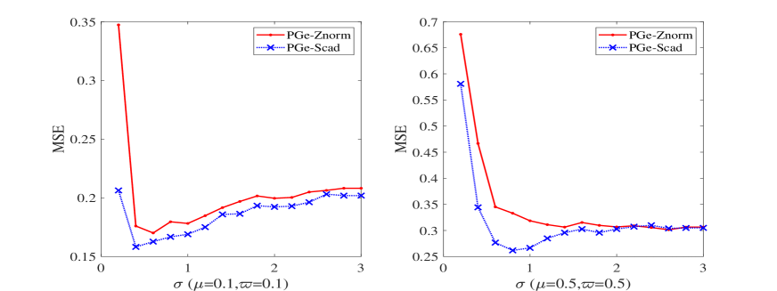
Figure 4: Influence of $\sigma$ on the performance of the models (7) and (9)

Next we take a closer look at the influence of $\lambda$ on the models (7) and (9). To this end, we generate the signal $x^{\rm true}$, the sampling matrix $\Phi$ of type I, and the observation $b$ with $(m,n,s^{*})=(500,1000,5)$ and $(\mu,\varpi)=(0.3,0.1)$, and then solve the model (7) associated to $\sigma=0.8,\gamma=0.05$ for each $\lambda\in\{1,3,5,\ldots,49\}$ with PGe-znorm and solve the model (9) associated to $\sigma=0.8,\gamma=0.05,\rho=10$ for each $\lambda\in\{0.5,1.5,2.5,\ldots,24.5\}$ with PGe-scad. Figure 5 plots the average MSE of $50$ trials for each $\lambda$. When $r=0.15$, the MSE from the model (7) has a small variation for $\lambda\in[7,49]$, while the MSE from the model (9) has a small variation for $\lambda\in[3,24.5]$. When $r=0.05$, the MSE from the model (7) has a small variation for $\lambda\in[5,49]$ and is relatively low for $\lambda\in[5,16]$, while the MSE from the model (9) has a tiny change for $\lambda\in[1.5,24.5]$. In view of this, we always choose $\lambda=8$ for the model (7), and choose $\lambda=4$ and $\lambda=8$ for the model (9) with $n\leq 5000$ and $n>5000$, respectively, in the subsequent experiments.

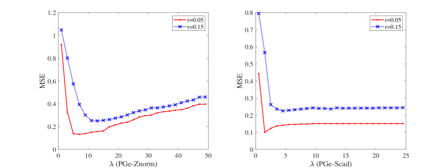
Figure 5: Influence of $\lambda$ on the MSE from the models (7) and (9)

5.4 Numerical comparisons

We compare PGe-znorm and PGe-scad with six state-of-the-art solvers, which are BIHT-AOP [46], PIHT [20], PIHT-AOP [21], GPSP [52] (https://github.com/ShenglongZhou/GPSP), PDASC [19] and WPDASC [15]. Among others, the codes for BIHT-AOP, PIHT and PIHT-AOP can be found at http://www.esat.kuleuven.be/stadius/ADB/huang/downloads/1bitCSLab.zip and the codes for PDASC and WPDASC can be found at https://github.com/cjia80/numericalSimulation. It is worth pointing out that BIHT-AOP, GPSP and PIHT-AOP all require an estimation on $s^{*}$ and $r$ as an input, PIHT require an estimation on $s^{*}$ as an input, while PDASC, WPDASC, PGe-znorm and PGe-scad do not need these prior information. For the solvers to require an estimation on $s^{*}$ and $r$, we directly input the true sparsity $s^{*}$ and $r$ as those papers do. During the testing, PGe-znorm and PGe-scad use the parameters described before, and other solvers use their default setting except the PIHT is terminated once its iteration is over $100$.

We first apply the eight solvers to solving the test problems with the sampling matrix of type I and low noise. Table 1 reports their average MSE, Herr, FNR, FPR and CPU time for $50$ trials. We see that among the four solvers without requiring any information on $x^{\rm true}$, PGe-scad and PGe-znorm yield the lower MSE, Herr and FNR than PDASC and WPDASC do, and PGe-scad is the best one in terms of MSE, Herr and FNR; while among the four solvers requiring some information on $x^{\rm true}$, BIHT-AOP and PIHT-AOP yield the smaller MSE and Herr than PIHT and GPSP do, and the former also yields the lower FNR and FPR under the scenario of $r=0.05$. When comparing PGe-scad with BIHT-AOP and PIHT-AOP, the former yields the smaller MSE, Herr, FNR and FPR under the scenario of $r=0.15$, and under the scenario of $r=0.05$, it also yields the comparable MSE, Herr and FNR as BIHT-AOP and PIHT-AOP do.

Table 1: Numerical comparisons of eight solvers for test problems with $\Phi$ of type I and low noise

$m=800,n=2000,s^{*}=10,\varpi=0.1,{\bf r=0.05}$

$\mu=0.1$

$\mu=0.3$

$\mu=0.5$

solvers

MSE

Herr

FNR

FPR

time(s)

MSE

Herr

FNR

FPR

time(s)

MSE

Herr

FNR

FPR

time(s)

PIHT

2.57e-1

6.80e-2

3.26e-1

1.64e-3

1.55e-1

2.75e-1

7.27e-2

3.52e-1

1.77e-3

1.57e-1

3.52e-1

9.22e-2

4.24e-1

2.13e-3

1.58e-1

BIHT-AOP

1.46e-1

4.36e-2

1.94e-1

9.75e-4

5.30e-1

1.32e-1

3.85e-2

1.80e-1

9.05e-4

5.47e-1

1.46e-1

4.18e-2

2.06e-1

1.04e-3

5.45e-1

PIHT-AOP

1.61e-1

4.67e-2

2.06e-1

1.04e-3

1.81e-1

1.55e-1

4.60e-2

1.90e-1

9.55e-4

1.92e-1

1.40e-1

4.17e-2

2.02e-1

1.02e-3

1.86e-1

GPSP

1.91e-1

5.02e-2

2.56e-1

1.29e-3

1.60e-2

1.87e-1

4.83e-2

2.40e-1

1.21e-3

1.83e-2

1.89e-1

4.78e-2

2.52e-1

1.27e-3

2.31e-2

PGe-scad

2.15e-1

6.70e-2

3.34e-1

0

2.29e-1

2.04e-1

6.36e-2

3.32e-1

0

2.79e-1

2.10e-1

6.42e-2

3.44e-1

1.01e-5

2.82e-1

PGe-znorm

2.10e-1

6.52e-2

3.58e-1

2.01e-5

1.19e-1

2.10e-1

6.41e-2

3.62e-1

4.02e-5

1.24e-1

2.22e-1

6.82e-2

3.72e-1

3.02e-5

1.26e-1

PDASC

4.29e-1

1.34e-1

5.94e-1

0

6.04e-2

4.27e-1

1.33e-1

5.92e-1

0

5.98e-2

4.53e-1

1.37e-1

6.08e-1

1.01e-5

5.93e-2

WPDASC

4.38e-1

1.37e-1

6.02e-1

0

9.31e-2

4.20e-1

1.30e-1

5.78e-1

0

9.32e-2

3.97e-1

1.20e-1

5.56e-1

1.01e-5

9.69e-2

$m=800,n=2000,s^{*}=10,\varpi=0.1,{\bf r=0.15}$

$\mu=0.1$

$\mu=0.3$

$\mu=0.5$

MSE

Herr

FNR

FPR

time(s)

MSE

Herr

FNR

FPR

time(s)

MSE

Herr

FNR

FPR

time(s)

PIHT

4.10e-1

1.13e-1

4.04e-1

2.03e-3

1.61e-1

4.01e-1

1.08e-1

2.90e-1

1.96e-3

1.57e-1

4.18e-1

1.12e-1

4.02e-1

2.02e-1

1.60e-1

BIHT-AOP

3.77e-1

1.04e-1

4.10e-1

2.06e-3

5.41e-1

3.74e-1

9.88e-2

4.16e-1

2.09e-3

5.51e-1

3.56e-1

9.49e-2

3.94e-1

1.98e-3

5.38e-1

PIHT-AOP

3.48e-1

9.80e-2

3.82e-1

1.92e-3

1.85e-1

3.70e-1

1.01e-1

4.10e-1

2.06e-3

1.91e-1

3.65e-1

9.68e-2

4.08e-1

2.05e-3

1.87e-1

GPSP

3.90e-1

1.05e-1

3.86e-1

1.94e-3

1.86e-2

3.73e-1

1.01e-1

3.76e-1

1.89e-3

2.04e-2

3.63e-1

9.31e-2

3.74e-1

1.88e-3

2.48e-2

PGe-scad

2.72e-1

8.54e-2

3.98e-1

1.51e-4

2.31e-1

2.78e-1

8.67e-2

3.90e-1

1.81e-4

2.83e-1

2.83e-1

8.39e-2

4.02e-1

1.91e-4

2.63e-1

PGe-znorm

3.33e-1

9.82e-2

4.20e-1

8.24e-4

1.34e-1

3.31e-1

9.64e-2

4.16e-1

9.45e-3

1.34e-1

3.42e-1

9.56e-2

4.14e-1

9.55e-4

1.50e-1

PDASC

5.63e-1

1.80e-1

6.88e-1

0

5.08e-2

5.89e-1

1.85e-1

7.12e-1

0

5.18e-2

5.58e-1

1.73e-1

6.90e-1

4.02e-5

5.18e-2

WPDASC

5.40e-1

1.71e-1

6.72e-1

0

7.93e-2

5.87e-1

1.83e-1

7.10e-1

1.01e-5

8.32e-2

5.63e-1

1.75e-1

6.98e-1

0

8.08e-2

Next we use the eight solvers to solve the test problems with the sampling matrix of type I and high noise. Table 2 reports the average MSE, Herr, FNR, FPR and CPU time for $50$ trials. Now among the four solvers requiring partial information on $x^{\rm true}$, GPSP yields the smallest MSE, Herr, FNR and FPR, and among the four solvers without requiring any information on $x^{\rm true}$, PGe-scad is still the best one. Also, for those problems with $r=0.15$, PGe-scad yields the smaller MSE, Herr and FNR than GPSP does.

Table 2: Numerical comparisons of eight solvers for test problems with $\Phi$ of type I and high noise

$m=1000,n=5000,s^{*}=15,\varpi=0.3,{\bf r=0.05}$

$\mu=0.1$

$\mu=0.3$

$\mu=0.5$

solvers

MSE

Herr

FNR

FPR

time(s)

MSE

Herr

FNR

FPR

time(s)

MSE

Herr

FNR

FPR

time(s)

PIHT

3.48e-1

9.53e-2

4.15e-1

1.25e-3

5.42e-1

3.40e-1

9.54e-2

4.19e-1

1.26e-3

5.46e-1

3.62e-1

9.67e-2

4.47e-1

1.34e-3

5.56e-1

BIHT-AOP

3.57e-1

1.11e-1

3.80e-1

1.14e-3

1.59e-0

3.47e-1

1.09e-1

3.67e-1

1.10e-3

1.60e-0

3.25e-1

1.05e-1

3.61e-1

1.09e-3

1.61e-0

PIHT-AOP

3.71e-1

1.17e-1

3.83e-1

1.15e-3

5.66e-1

3.47e-1

1.10e-1

3.71e-1

1.11e-3

5.79e-1

3.30e-1

1.10e-1

3.59e-1

1.08e-3

5.83e-1

GPSP

2.64e-1

7.33e-2

3.31e-1

9.95e-4

5.77e-2

2.68e-1

7.52e-2

3.32e-1

9.99e-4

5.19e-2

2.95e-1

8.08e-2

3.63e-1

1.09e-3

4.89e-2

PGe-scad

2.65e-1

8.36e-2

3.87e-1

2.21e-4

1.05e-0

2.67e-1

8.35e-2

3.85e-1

2.45e-4

1.01e-0

2.65e-1

8.13e-2

3.93e-1

2.29e-4

1.10e-0

PGe-znorm

2.89e-1

8.85e-2

4.67e-1

8.83e-5

4.05e-1

2.92e-1

8.89e-2

4.69e-1

7.22e-5

4.17e-1

3.00e-1

8.95e-2

4.77e-1

9.63e-5

4.20e-1

PDASC

5.55e-1

1.77e-1

7.24e-1

0

1.63e-1

5.80e-1

1.84e-1

7.44e-1

0

1.64e-1

5.96e-1

1.89e-1

7.48e-1

4.01e-6

1.65e-1

WPDASC

5.73e-1

1.84e-1

7.36e-1

0

2.66e-1

5.54e-1

1.76e-1

7.19e-1

0

2.68e-1

5.96e-1

1.88e-1

7.49e-1

0

2.70e-1

$m=1000,n=5000,s^{*}=15,\varpi=0.3,{\bf r=0.15}$

$\mu=0.1$

$\mu=0.3$

$\mu=0.5$

MSE

Herr

FNR

FPR

time(s)

MSE

Herr

FNR

FPR

time(s)

MSE

Herr

FNR

FPR

time(s)

PIHT

5.28e-1

1.48e-1

4.97e-1

1.50e-3

5.52e-1

5.42e-1

1.51e-1

5.09e-1

1.53e-3

5.50e-1

5.30e-1

1.47e-1

4.81e-1

1.45e-3

5.46e-1

BIHT-AOP

5.23e-1

1.51e-1

5.13e-1

1.54e-3

1.61e-0

4.97e-1

1.45e-1

5.00e-1

1.50e-3

1.60e-0

5.19e-1

1.46e-1

5.35e-1

1.61e-3

1.61e-0

PIHT-AOP

5.13e-1

1.46e-1

5.09e-1

1.53e-3

5.78e-1

5.04e-1

1.47e-1

5.13e-1

1.54e-3

5.79e-1

5.30e-1

1.52e-1

5.45e-1

1.64e-3

5.70e-1

GPSP

4.60e-1

1.29e-1

4.59e-1

1.38e-3

8.21e-2

4.60e-1

1.29e-1

4.65e-1

1.40e-3

8.13e-2

4.90e-1

1.33e-1

4.77e-1

1.44e-3

6.03e-2

PGe-scad

3.55e-1

1.09e-1

4.76e-1

1.34e-3

1.05e-0

3.63e-1

1.12e-1

4.81e-1

1.50e-3

1.11e-0

3.63e-1

1.12e-1

4.80e-1

1.38e-3

1.27e-0

PGe-znorm

4.22e-1

1.24e-2

5.17e-1

6.38e-4

4.19e-1

4.51e-1

1.30e-1

5.19e-1

7.94e-4

4.06e-1

4.41e-1

1.27e-1

5.21e-1

6.62e-4

4.49e-1

PDASC

6.90e-1

2.24e-1

8.12e-1

4.01e-6

1.35e-1

7.07e-1

2.26e-1

8.24e-1

4.01e-6

1.34e-1

7.11e-1

2.27e-1

8.27e-1

0

1.33e-1

WPDASC

6.62e-1

2.14e-1

7.92e-1

0

2.35e-1

6.82e-1

2.18e-1

8.03e-1

4.01e-6

2.34e-1

7.04e-1

2.25e-1

8.20e-1

4.01e-6

2.30e-1

Finally, we use the eight solvers to solve the test problems with the sampling matrix of type II. Table 3 reports the average MSE, Herr, FNR, FPR and CPU time for $50$ trials. From Table 3, among the four solvers requiring partial information on $x^{\rm true}$, PIHT yields the better MSE, Herr,FNR and FPR than others for those examples with high noise, and among the four solvers without needing any information on $x^{\rm true}$, PGe-scad is still the best one. Moreover, PGe-scad yields the smaller MSE, Herr and FNR than PIHT does for $\varpi=0.3$ and $0.5$. We also observe that among the eight solvers, GPSP always requires the least CPU time, and PGe-scad and PGe-znorm requires the comparable CPU time as PIHT, BIHT-AOP and PIHT-AOP do for all test examples.

Table 3: Numerical comparisons of eight solvers for test problems with $\Phi$ of type II with different noise levels

$m=2500,n=10000,s^{*}=20,r=0.1$

$\varpi=0.1$

$\varpi=0.3$

$\varpi=0.5$

MSE

Herr

FNR

FPR

time(s)

MSE

Herr

FNR

FPR

time(s)

MSE

Herr

FNR

FPR

time(s)

PIHT

2.57e-1

7.23e-1

3.44e-1

6.89e-4

2.55

2.74e-1

8.15e-2

3.49e-1

6.99e-4

2.54

3.14e-1

9.58e-2

3.69e-1

7.39e-4

2.54

BIHT-AOP

1.54e-1

4.61e-2

2.40e-1

4.81e-4

7.70

3.06e-1

9.84e-2

3.36e-1

6.73e-3

7.68

4.23e-1

1.29e-1

3.95e-1

7.92e-4

7.64

PIHT-AOP

1.68e-1

5.08e-2

2.44e-1

4.89e-4

2.66

3.16e-1

1.03e-1

3.38e-1

6.77e-4

2.66

4.62e-1

1.52e-1

4.14e-1

8.30e-4

2.66

GPSP

2.45e-1

6.88e-2

3.36e-1

6.73e-4

0.19

2.77e-1

8.22e-2

3.51e-1

7.03e-4

0.19

3.23e-1

9.68e-2

3.73e-1

7.47e-4

0.19

PGe-scad

2.10e-1

6.65e-2

3.08e-1

2.61e-5

2.79

2.44e-1

7.82e-2

3.61e-1

2.10e-4

2.71

2.92e-1

9.34e-2

4.14e-1

6.89e-4

2.75

PGe-znorm

2.34e-1

7.36e-2

4.25e-1

2.00e-6

1.78

2.44e-1

7.71e-2

4.27e-1

8.02e-6

1.78

2.74e-1

8.70e-2

4.45e-1

3.21e-5

1.77

PDASC

5.41e-1

1.73e-1

6.84e-1

0

8.28e-1

6.26e-1

2.01e-1

7.50e-1

0

8.07e-1

6.28e-1

2.03e-1

7.56e-1

4.02e-5

7.66e-1

WPDASC

5.41e-1

1.73e-1

6.83e-1

0

1.01

5.62e-1

1.81e-1

7.03e-1

0

9.98e-1

6.17e-1

1.99e-1

7.37e-1

0

9.71e-1

6 Conclusion

We proposed a zero-norm regularized smooth DC loss model and derived a family of equivalent nonconvex surrogates that cover the MCP and SCAD surrogates as special cases. For the proposed model and its SCAD surrogate, we developed the PG method with extrapolation to compute their $\tau$-stationary points and provided its convergence certificate by establishing the convergence of the whole iterate sequence and its local linear convergence rate. Numerical comparisons with several state-of-art methods demonstrate that the two new models are well suited for high noise and/or high sign flip ratio. An interesting future topic is to analyze the statistical error bound for them.

References

- [1] H. Attouch and J. Bolte, On the convergence of the proximal algorithm for nonsmooth functions involving analytic features, Mathematical Programming, 116(2009): 5-16.
- [2] H. Attouch, J. Bolte, P. Redont and A. Soubeyran, Proximal alternating minimization and projection methods for nonconvex problems: an approach based on the Kurdyka-Łojasiewicz inequality, Mathematics of Operations Research, 35(2010): 438-457.
- [3] A. Beck and M. Teboulle, Fast gradient-based algorithms for constrained total variation image denoising and deblurring problems, IEEE Transactions on Image Processing, 18(2009): 2419-2434.
- [4] A. Beck and N. Hallak, Optimization problems involving group sparsity terms, Mathematical Programming, 178(2019): 39-67.
- [5] J. Bolte, S. Sabach and M. Teboulle, Proximal alternating linearized minimization for nonconvex and nonsmooth problems, Mathematical Programming, 146(2014): 459-494.
- [6] P. T. Boufounos and R. G. Baraniuk, 1-bit compressive sensing, Proceedings of the Forty Second Annual Conference on Information Sciences and Systems, 2008, pp. 16-21.
- [7] P. T. Boufounos, Greedy sparse signal reconstruction from sign measurements, Proceedings of the Asilomar Conference on Signals, Systems, and Computers, 2009: 1305-1309.
- [8] P. T. Boufounos, Reconstruction of sparse signals from distorted randomized measurements, In Proceedings of the IEEE International Conference on Acoustics Speech and Signal Processing, 2010, pp. 3998-4001.
- [9] J. P. Brooks, Support vector machines with the ramp Loss and the hard margin loss, Operations Research, 59(2011): 467-479.
- [10] E. J. Candès and T. Tao, Decoding by linear programming, IEEE Transactions on Information Theory, 51(2005): 4203-4215.
- [11] F. Cucker and D. X. Zhou, Learning Theory: An Approximation Theory Viewpoint, Cambridge, U.K.: Cambridge Univ. Press, 2007.
- [12] D. Q. Dai, L. X. Shen, Y. S. Xu and N. Zhang, Noisy 1-bit compressive sensing: models and algorithms, Applied and Computational Harmonic Analysis, 40(2016): 1-32.
- [13] D. L. Donoho, Compressed sensing, IEEE Transactions on Information Theory, 52(2006): 1289-1306.
- [14] J. Q. Fan and R. Z. Li, Variable selection via nonconcave penalized likelihood and its oracle properties, Journal of American Statistics Association, 96(2001): 1348-1360.
- [15] Q. B. Fan, C. Jia, J. Liu and Y. Luo, Robust recovery in 1-bit compressive sensing via -constrained least squares, Signal Processing, 179(2021): 107822.
- [16] J. Fang, Y. N. Shen, H. B. Li and Z. Ren, Sparse signal recovery from one-bit quantized data: an iterative reweighted algorithm, Signal Processing, 102(2014): 201-206.
- [17] S. Ghadimi and G. Lan, Accelerated gradient methods for nonconvex nonlinear and stochastic programming, Mathematical Programming, 156(2016):59-99.
- [18] S. Gopi, P. Netrapalli, P. Jain and A. Nori, One-bit compressed sensing: Provable support and vector recovery, in Int. Conf. Mach. Learn. PMLR, 2013, pp. 154-162.
- [19] J. Huang, Y. L. Jiao, X. L. Lu and L. P. Zhu, Robust decoding from 1-bit compressive sampling with ordinary and regularized least squares, SIAM Journal on Scientific Computing, 40(2018): A2062-A2086.
- [20] X. L. Huang and M. Yan, Nonconvex penalties with analytical solutions for one-bit compressive sensing, Signal Processing, 144(2018): 341-351.
- [21] X. L. Huang, L. Shi, M. Yan and J. A. K. Suykens, Pinball loss minimization for one-bit compressive sensing: convex models and algorithms, Neurocomputing, 314(2018): 275-283.
- [22] X. L. Huang, L. Shi and J. A. K. Suykens, Ramp loss linear programming support vector machine, Journal of Machine Learning Research, 15(2014): 2185-2211.
- [23] L. Jacques, J. N. Laska, P. T. Boufounos and R. G. Baraniuk, Robust 1-bit compressive sensing via binary stable embeddings of sparse vectors, IEEE Transactions on Information Theory, 59(2013): 2082-2102.
- [24] J. N. Laska, Z. W. Wen, W. T. Yin and R. G. Baraniuk, Trust, but verify: fast and accurate signal recovery from 1-bit compressive measurements, IEEE Transactions on Signal Processing, 59(2011): 5289-5301.
- [25] J. N. Laska and R. G. Baraniuk, Regime change: Bitdepth versus measurement-rate in compressive sensing, IEEE Transactions on Signal Processing, 60(2012): 3496-3505.
- [26] Z. L. Li, W. B. Xu, X. B. Zhang and J. R. Lin, A survey on one-bit compressed sensing: theory and applications, Frontiers of Computer Science, 12(2018): 217-230.
- [27] H. Li and Z. Lin, Accelerated proximal gradient methods for nonconvex programming, In Advances in Neural Information Processing Systems, 2015: 379-387.
- [28] P. Ochs, Unifying abstract inexact convergence theorems and block coordiate variable metric IPIANO, SIAM Journal on Optimization, 29(2019): 511-570.
- [29] P. Ochs, Y. Chen, T. Brox and T. Pock, iPiano: Inertial proximal algorithm for nonconvex optimization, SIAM Journal on Optimization, 7(2014): 1388-1419.
- [30] Y. Plan and R. Vershynin, One-bit compressed sensing by linear programming, Communications on Pure and Applied Mathematics, 66(2013): 1275-1297.
- [31] Y. Plan and R. Vershynin, Robust 1-bit compressed sensing and sparse logistic regression: a convex programming approach, IEEE Transactions on Information Theory, 59(2013): 482-494.
- [32] X. Peng, B. Liao and J. Li, One-bit compressive sensing via Schur-concave function minimization, IEEE Transactions on Signal Processing, 67(2019): 4139-4151.
- [33] X. Peng, B. Liao, X. D. Huang and Z. Quan, 1-bit compressive sensing with an improved algorithm based on fixed-point continuation, Signal Processing, 154(2019): 168-173.
- [34] G. Y. Li and T. K. Pong, Calculus of the exponent of Kurdyka-Łöjasiewicz inequality and its applications to linear convergence of first-order methods, Foundations of Computational Mathematics, 18(2018): 1199-1232.
- [35] Y. L. Liu, S. J. Bi and S. H. Pan, Equivalent Lipschitz surrogates for zero-norm and rank optimization problems, Journal of Global Optimization, 72(2018): 679-704.
- [36] R. T. Rockafellar and R. J-B. Wets, Variational Analysis, Springer, 1998.
- [37] Y. Nesterov, A method of solving a convex programming problem with convergence rate , Soviet Mathematics Doklady, 27: 372-376, 1983.
- [38] Y. Nesterov, Introductory Lectures on Convex Optimization: A Basic Course, Kluwer Academic Publishers, Boston, 2004.
- [39] Y. T. Qian and S. H. Pan, Calmness of partial perturbation to composite rank constraint systems and its applications, arXiv:2102.10373v2, October 8, 2021.
- [40] L. X. Shen and B. W. Suter, One-bit compressive sampling via minimization, EURASIP Journal on Advances in Signal Processing, 71(2016).
- [41] B. Wen, X. Chen, and T. K. Pong, Linear convergence of proximal gradient algorithm with extrapolation for a class of nonconvex nonsmooth minimization problems, SIAM Journal on Optimization, 27(2017): 124-145.
- [42] Y. Q. Wu, S. H. Pan and S. J. Bi, Kurdyka-Łojasiewicz property of zero-norm composite functions, Journal of Optimization Theory and Applications, 188(2021): 94-112.
- [43] H. Wang, X. Huang, Y. Liu, H. Sabine Van and W. Qun, Binary reweighted l1-norm minimization for one-bit compressed sensing, In 8th International Conference on Bio-inspired Systems & Signal Processing, 2015.
- [44] P. Xiao, B. Liao and J. Li, One-bit compressive sensing via Schur-concave function minimization, IEEE Transactions on Signal Processing, 16(2019): 4139-4151.
- [45] Y. Y. Xu and W. Yin, A globally convergent algorithm for nonconvex optimization based on block coordinate update, Journal of Scientific Computing, 72(2017): 700-734.
- [46] M. Yan, Y. Yang and S. Osher, Robust 1-bit compressive sensing using adaptive outlier pursuit, IEEE Transactions on Signal Processing, 60(2012): 3868-3875.
- [47] L. Yang, Proximal gradient method with extrapolation and line-search for a class of nonconvex and nonsmooth problems, arXiv:1711.06831v4, 2021.
- [48] P. R. Yu, G. Y. Li and T. K. Pong, Kurdyka-Łöjasiewicz exponent via inf-projection, Foundations of Computational Mathematics, DOI: https://doi.org/10.1007/s10208-021-09528-6.
- [49] C. H. Zhang, Nearly unbiased variable selection under minimax concave penalty, Annals of Statistics, 38(2010): 894-942.
- [50] T. Zhang, Statistical analysis of some multi-category large margin classification methods, Journal of Machine Learning Research, 5(2004): 1225-1251.
- [51] L. Zhang, J. Yi and R. Jin, Efficient algorithms for robust one-bit compressive sensing, Proceedings of the thirty First International Conference on Machine Learning, 2014, pp. 820-828.
- [52] S. L. Zhou, Z. Y. Luo, N. H. Xiu and G. Y. Li, Computing One-bit compressive sensing via double-sparsity constrained optimization, Journal of Machine Learning Research, 5(2004): 1225-1251.
- [53] R. D. Zhu and Q. Q. Gu, Towards a lower sample complexity for robust one-bit compressed sensing, Proceedings of the 32nd International Conference on Machine Learning, PMLR, 37(2015): 739-747.