SRFormer: Permuted Self-Attention for Single Image Super-Resolution

Abstract

Previous works have shown that increasing the window size for Transformer-based image super-resolution models (e.g., SwinIR) can significantly improve the model performance but the computation overhead is also considerable. In this paper, we present SRFormer, a simple but novel method that can enjoy the benefit of large window self-attention but introduces even less computational burden. The core of our SRFormer is the permuted self-attention (PSA), which strikes an appropriate balance between the channel and spatial information for self-attention. Our PSA is simple and can be easily applied to existing super-resolution networks based on window self-attention. Without any bells and whistles, we show that our SRFormer achieves a 33.86dB PSNR score on the Urban100 dataset, which is 0.46dB higher than that of SwinIR but uses fewer parameters and computations. We hope our simple and effective approach can serve as a useful tool for future research in super-resolution model design.

1 Introduction

Single image super-resolution (SR) aims to restore a high-quality image from its degraded low-resolution version. Exploring efficient and effective super-resolution algorithms has been a hot research topic in computer vision, which have a variety of applications [23, 59, 2]. Since the pioneer works [9, 24, 75, 28, 48, 34], CNN-based methods have been the mainstream for image super-resolution for a long time. These methods mostly take advantage of residual learning [51, 28, 34, 24, 73, 30], dense connections [63, 79, 54], or channel attention [78, 66] to construct network architectures, making great contributions to the development of super-resolution models.

Figure 1: Performance comparison between SwinIR and our SRFormer when training 200k iterations with different window sizes (WS) for 200k iterations. Our SRFormer enjoys a large window size of $24\times 24$ with even fewer computations but higher PSNR scores.

Despite the success made by CNN-based models in super-resolution, recent works [5, 33, 72, 77] have shown that Transformer-based models perform better. They observe that the ability of self-attention to build pairwise relationships is a more efficient way to produce high-quality super-resolution images than convolutions. One typical work among them should be SwinIR [33] which introduces Swin Transformer [37] to image super-resolution, greatly improving the state-of-the-art CNN-based models on various benchmarks. Later, a variety of works, such as SwinFIR [72], ELAN [77], and HAT [6], further develop SwinIR and use Transformers to design different network architectures for SR.

The aforementioned methods reveal that properly enlarging the windows for the shifted window self-attention in SwinIR can result in clear performance gain (see Figure 1). However, the computational burden is also an important issue as the window size goes larger. In addition, Transformer-based methods utilize self-attention and require networks of larger channel numbers compared to previous CNN-based methods [78, 79, 24]. To explore efficient and effective super-resolution algorithms, a straightforward question should be: How would the performance go if we reduce the channel number and meanwhile increase the window size?

Motivated by the question mentioned above, in this paper, we present permuted self-attention (PSA), an efficient way to build pairwise relationships within large windows (e.g., $24\times 24$). The intention is to enable more pixels to get involved in the attention map computation and at the same time introduce no extra computational burden. To this end, we propose to shrink the channel dimensions of the key and value matrices and adopt a permutation operation to convey part of the spatial information into the channel dimension. In this way, despite the channel reduction, there is no loss of spatial information, and each attention head is also allowed to keep a proper number of channels to produce expressive attention maps [56]. In addition, we also improve the original feed-forward network (FFN) by adding a depth-wise convolution between the two linear layers, which we found helps in high-frequency component recovery.

Given the proposed PSA, we construct a new network for SR, termed SRFormer. We evaluate our SRFormer on five widely-used datasets. Benefiting from the proposed PSA, our SRFormer can clearly improve its performance on almost all five datasets. Notably, for $\times 2$ SR, our SRFormer trained on only the DIV2K dataset [34] achieves a 33.86 PSNR score on the challenging Urban100 dataset [18]. This result is much higher than those of the recent SwinIR (33.40) and ELAN (33.44). A similar phenomenon can also be observed when evaluating on the $\times 3$ and $\times 4$ SR tasks. In addition, we perform experiments using a light version of our SRFormer. Compared to previous lightweight SR models, our method also achieves better performance on all benchmarks.

To sum up, our contributions can be summarized as follows:

• We propose a novel permuted self-attention for image super-resolution, which can enjoy large-window self-attention by transferring spatial information into the channel dimension. By leveraging it, we are the first to implement 24x24 large window attention mechanism at an acceptable time complexity in SR.

• We build a new transformer-based super-resolution network, dubbed SRFormer, based on the proposed PSA and an improved FFN from the frequency perspective (ConvFFN). Our SRFormer achieves state-of-the-art performance in classical, lightweight, and real-world image SR tasks.

2 Related Work

In this section, we briefly review the literature on image super-resolution. We first describe CNN-based methods and then transition to the recent popular Transformer-based models.

2.1 CNN-Based Image Super-Resolution

Since SRCNN[9] first introduced CNN into image super-resolution (SR), a large number of CNN-based SR models have emerged. DRCN [25] and DRRN [51] introduce recursive convolutional networks to increase the depth of the network without increasing the parameters. Some early CNN-based methods [52, 9, 25, 51] attempt to interpolate the low-resolution (LR) as input, which results in a computationally expensive feature extraction. To accelerate the SR inference process, FSRCNN [10] extracts features at the LR scale and conducts an upsampling operation at the end of the network. This pipeline with pixel shuffle upsampling [48] has been widely used in later works [77, 78, 33]. LapSRN [27] and DBPN [17] perform upsampling during extracting feature to learn the correlation between LR and HR. There are also some works [28, 63, 76, 61] that use GAN [14] to generate realistic textures in reconstruction. MemNet [52], RDN [79], and HAN [45] efficiently aggregate the intermediate features to enhance the quality of the reconstructed images. Non-Local attention [60] has also been extensively explored in SR to better model the long-range dependencies. Methods of this type include CS-NL [44], NLSA [43], SAN [7], IGNN [81], etc.

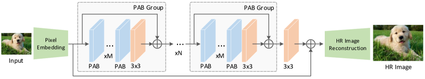
Figure 2: Overall architecture of SRFormer. The pixel embedding module is a $3\times 3$ convolution to map the input image to feature space. The HR image reconstruction module contains a $3\times 3$ convolution and a pixel shuffle operation to reconstruct the high-resolution image. The middle feature encoding part has $N$ PAB groups, followed by a $3\times 3$ convolution.

2.2 Vision Transformers

Transformers recently have shown great potential in a variety of vision tasks, including image classification [11, 55, 67, 58, 68], object detection [4, 50, 12], semantic segmentation [65, 80, 49], image restoration [69, 33, 5], etc. Among these, the most typical work should be Vision Transformer (ViT) [11] which proves Transformers can perform better than convolutional neural networks on feature encoding. The application of Transformers in low-level vision mainly includes two categories: generation [22, 29, 71, 8] and restoration. Further, the restoration tasks can also be divided into two categories: video restoration [38, 36, 47, 35, 13] and image restoration [5, 69, 64, 16].

As an important task in image restoration, image super-resolution needs to preserve the structural information of the input, which is a great challenge for Transformer-based model design. IPT [5] is a large pre-trained model based on the Transformer encoder and decoder structure and has been applied to super-resolution, denoising, and deraining. Based on the Swin Transformer encoder [37], SwinIR [33] performs self-attention on an $8\times 8$ local window in feature extraction and achieves extremely powerful performance. ELAN [77] simplifies the architecture of SwinIR and uses self-attention computed in different window sizes to collect the correlations between long-range pixels.

Our SRFormer is also based on Transformer. Different from the aforementioned methods that directly leverage self-attention to build models, our SRFormer mainly aims at the self-attention itself. Our intention is to study how to compute self-attention in a large window to improve the performance of SR models without increasing the parameters and computational cost.

3 Method

3.1 Overall Architecture

The overall architecture of our SRFormer is shown in Fig. 2, consisting of three parts: a pixel embedding layer $G_{P}$, a feature encoder $G_{E}$, and a high-resolution image reconstruction layer $G_{R}$. Following previous works [33, 77], the pixel embedding layer $G_{P}$ is a single $3\times 3$ convolution that transforms the low-resolution RGB image $I\in\mathbb{R}^{H\times W\times 3}$ to feature embeddings $F_{P}\in\mathbb{R}^{H\times W\times C}$. $F_{P}$ will then be sent into the feature encoder $G_{E}$ with a hierarchical structure. It consists of $N$ permuted self-attention groups, each of which is with $M$ permuted self-attention blocks followed by a $3\times 3$ convolution. A $3\times 3$ convolution is added at the end of the feature encoder, yielding $F_{E}$. The summation results of $F_{E}$ and $F_{P}$ are fed into $G_{R}$ for high-resolution image reconstruction, which contains a $3\times 3$ convolution and a sub-pixel convolutional layer [48] to reconstruct high-resolution images. We compute the L1 loss between the high-resolution reconstructed image and ground-truth HR image to optimize our SRFormer.

Figure 3: Comparison between (a) self-attention and (b) our proposed permuted self-attention. To avoid spatial information loss, we propose to reduce the channel numbers and transfer the spatial information to the channel dimension.

3.2 Permuted Self-Attention Block

The core of our SRFormer is the permuted self-attention block (PAB), which consists of a permuted self-attention (PSA) layer and a convolutional feed-forward network (ConvFFN).

Permuted self-attention. As shown in Fig. 3(b), given an input feature map $\mathbf{X}_{in}\in\mathbb{R}^{H\times W\times C}$ and a tokens reduction factor $r$, we first split $\mathbf{X}_{in}$ into $N$ non-overlapping square windows $\mathbf{X}\in\mathbb{R}^{NS^{2}\times C}$, where $S$ is the side length of each window. Then, we use three linear layers $L_{Q},L_{K},L_{V}$ to get $\mathbf{Q}$, $\mathbf{K}$, and $\mathbf{V}$:

$$\mathbf{Q},\mathbf{K},\mathbf{V}=L_{Q}(\mathbf{X}),L_{K}(\mathbf{X}),L_{V}(\mathbf{X}).$$ (1)

Here, $\mathbf{Q}$ keeps the same channel dimension to $\mathbf{X}$ while $L_{K}$ and $L_{V}$ compress the channel dimension to $C/r^{2}$, yielding $\mathbf{K}\in\mathbb{R}^{NS^{2}\times C/r^{2}}$ and $\mathbf{V}\in\mathbb{R}^{NS^{2}\times C/r^{2}}$. After that, to enable more tokens to get involved in the self-attention calculation and avoid the increase of the computational cost, we propose to permute the spatial tokens in $\mathbf{K}$ and $\mathbf{V}$ to the channel dimension, attaining permuted tokens $\mathbf{K}_{p}\in\mathbb{R}^{NS^{2}/r^{2}\times C}$ and $\mathbf{V}_{p}\in\mathbb{R}^{NS^{2}/r^{2}\times C}$.

We use $\mathbf{Q}$ and the shrunken $\mathbf{K}_{p}$ and $\mathbf{V}_{p}$ to perform the self-attention operation. In this way, the window size for $\mathbf{K}_{p}$ and $\mathbf{V}_{p}$ will be reduced to $\frac{S}{r}\times\frac{S}{r}$ but their channel dimension is still unchanged to guarantee the expressiveness of the attention map generated by each attention head [56]. The formulation of the proposed PSA can be written as follows:

$$\operatorname{PSA}(\mathbf{Q},\mathbf{K}_{p},\mathbf{V}_{p})=\operatorname{Softmax}\left(\frac{\mathbf{Q}\mathbf{K}_{p}^{T}}{\sqrt{d_{k}}}+\mathbf{B}\right)\mathbf{V}_{p},$$ (2)

where $\mathbf{B}$ is an aligned relative position embedding that can be attained by interpolating the original one defined in [37] since the window size of $\mathbf{Q}$ does not match that of $\mathbf{K}_{p}$. $\sqrt{d_{k}}$ is a scalar as defined in [11]. Note that the above equation can easily be converted to the multi-head version by splitting the channels into multiple groups.

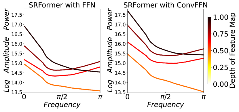
Figure 4: Power spectrum of the intermediate feature maps produced by our SRFormer with FFN and ConvFFN. Lines in darker color correspond to features from deeper layers.

Our PSA transfers the spatial information to the channel dimension. It ensures the following two key design principles: i) We do not downsample the tokens first as done in [65, 58] but allow each token to participate in the self-attention computation independently. This enables more representative attention maps. We will discuss more variants of our PSA in Sec. 3.3 and show more results in our experiment section. ii) In contrast to the original self-attention illustrated in Fig. 3(a), PSA can be conducted in a large window (e.g., $24\times 24$) using even fewer computations than SwinIR with $8\times 8$ window while attaining better performance.

ConvFFN. Previous works have demonstrated that self-attention can be viewed as a low-pass filter [46, 57]. To better restore high-frequency information, a $3\times 3$ convolution is often added at the end of each group of Transformers as done in SwinIR [33]. Different from SwinIR, in our PAB, we propose to add a local depthwise convolution branch between the two linear layers of the FFN block to assist in encoding more details. We name the new block as ConvFFN. We empirically found that such an operation increases nearly no computations but can compensate for the loss of high-frequency information caused by self-attention shown in Fig. 4. We simply calculate the power spectrum of the feature maps produced by our SRFormer with FFN and ConvFFN. By comparing the two figures, we can see that ConvFFN can clearly increase high-frequency information, and hence yields better results as listed in Tab. 1.

3.3 Large-Window Self-Attention Variants

To provide guidance for the design of large-window self-attention and demonstrate the advantage of our PSA, here, we introduce another two large-window self-attention variants. The quantitative comparisons and analysis can be found in our experiment section.

Token Reduction. The first way to introduce large-window self-attention and avoid the increase in computational cost is to reduce the number of tokens as done in [65]. Let $r$ and $S$ be a reduction factor and the window size. Given an input $\mathbf{X}\in\mathbb{R}^{NS^{2}\times C}$, we can adopt a depthwise convolutional function with kernel size $r\times r$ and stride $r$ to reduce the token numbers of $\mathbf{K}$ and $\mathbf{V}$ in each window to $(\frac{S}{r})^{2}$, yielding $\mathbf{Q}_{r}\in\mathbb{R}^{NS^{2}\times C}$ and $\mathbf{K}_{r}\in\mathbb{R}^{NS^{2}/r^{2}\times C}$. $\mathbf{Q}_{r}$ and $\mathbf{K}_{r}$ are used to compute the attention scores $\mathbf{A}\in\mathbb{R}^{{S^{2}}\times{S^{2}/r^{2}}}$. Computing the matrix multiplication between $\mathbf{A}$ and $\mathbf{V}$ yields the output with the same number of tokens to $\mathbf{X}$.

Token Sampling. The second way to achieve large-window self-attention is to randomly sample $T^{2}~{}(0\leq T\leq S)$ tokens from each window according to a given sampling ratio $t$ for the key $\mathbf{K}$ and value $\mathbf{V}$. Given the input $\mathbf{X}\in\mathbb{R}^{NS^{2}\times C}$, $\mathbf{Q}$ shares the same shape with $\mathbf{X}$ but the shapes of $\mathbf{K}$ and $\mathbf{V}$ are reduced to $NT^{2}\times C$. In this way, as long as $T$ is fixed, the computational cost increases linearly as the window size gets larger. A drawback of token sampling is that randomly selecting a portion of tokens loses structural information of the scene content, which is essentially needed for image super-resolution. We will show more numerical results in our experiment section.

Method	Window size	Params	MACs	SET5 [3]		SET14 [70]		B100 [41]		Urban100 [18]		Manga109 [42]
				PSNR	SSIM	PSNR	SSIM	PSNR	SSIM	PSNR	SSIM	PSNR	SSIM
SwinIR [33]	$8\times 8$	11.75M	2868G	38.24	0.9615	33.94	0.9212	32.39	0.9023	33.09	0.9373	39.34	0.9784
	$12\times 12$	11.82M	3107G	38.30	0.9617	34.04	0.9220	32.42	0.9026	33.28	0.9381	39.44	0.9788
	$16\times 16$	11.91M	3441G	38.32	0.9618	34.00	0.9212	32.44	0.9030	33.40	0.9394	39.53	0.9791
SRFormer w/o ConvFFN	$12\times 12$	9.97M	2381G	38.23	0.9615	34.00	0.9216	32.37	0.9023	32.99	0.9367	39.30	0.9786
	$16\times 16$	9.99M	2465G	38.25	0.9616	33.98	0.9209	32.38	0.9022	33.09	0.9371	39.42	0.9789
	$24\times 24$	10.06M	2703G	38.30	0.9618	34.08	0.9225	32.43	0.9030	33.38	0.9397	39.44	0.9786
SRFormer	$12\times 12$	10.31M	2419G	38.22	0.9614	34.08	0.9220	32.38	0.9025	33.08	0.9372	39.13	0.9780
	$16\times 16$	10.33M	2502G	38.31	0.9617	34.10	0.9217	32.43	0.9026	33.26	0.9385	39.36	0.9785
	$24\times 24$	10.40M	2741G	38.33	0.9618	34.13	0.9228	32.44	0.9030	33.51	0.9405	39.49	0.9788

Table 1: Ablation study on the window size. We report results on the original SwinIR, SRFormer without ConvFFN, and our full SRFormer. Note that the parameters and MACs of SRFormer with $24\times 24$ window are fewer than SwinIR with $8\times 8$ window. Larger windows can result in better performance.

ConvFFN	Urban100 [18]		Manga109 [42]
	PSNR	SSIM	PSNR	SSIM
w/o Depth-wise Conv	33.38	0.9397	39.44	0.9786
$3\times 3$ Depth-wise Conv	33.42	0.9398	39.34	0.9787
$5\times 5$ Depth-wise Conv	33.51	0.9405	39.49	0.9788

Table 2: Ablation study on ConvFFN for $\times$2 SR. From the results on Urban100 and Manga109, we can see that using $5\times 5$ depthwise convolution yields the best results. This indicates that local details are also essential for Transformer-based models.

Method	Params	MACs	$S$	$r$	PSNR	SSIM
SwinIR [33]	11.75M	2868G	8	-	33.09	0.9373
Token Reduction	11,78M	2471G	16	2	33.09	0.9372
Token Reduction	11.85M	2709G	24	2	33.24	0.9387
Token Sampling	11.91M	2465G	16	2	32.38	0.9312
Token Sampling	12.18M	2703G	24	2	32.34	0.9305
PSA	9.99M	2465G	16	2	33.09	0.9371
PSA	10.06M	2703G	24	2	33.38	0.9397

Table 3: $\times 2$ SR performance comparison among SwinIR [33], our proposed PSA, and the two variants on Urban100 [18]. The results reported here are based on the best model trained on DIV2K for 200k iterations. For token sampling, $r=S/T$. PSA performs better than another two variants.

4 Experiments

In this section, we conduct experiments on both the classical, lightweight, and real-world image SR tasks, compare our SRFormer with existing state-of-the-art methods, and do ablation analysis of the proposed method.

4.1 Experimental Setup

Datasets and Evaluation. The choice of training datasets keeps the same as the comparison models. In classical image SR, we use DIV2K [34] and DF2K (DIV2K [34] + Flickr2K [53]) to train two versions SRFormer. In lightweight image SR, we use DIV2K [34] to train our SRFormer-light. In real-world SR, We use DF2K and OST [62]. For testing, we mainly evaluate our method on five benchmark datasets, including Set5 [3], Set14 [70], BSD100 [41], Urban100 [18], and Manga109 [42]. Self-ensemble strategy is introduced to further improve performance, named SRFormer+. The experimental results are evaluated in terms of PSNR and SSIM values, which are calculated on the Y channel from the YCbCr space.

Implementation Details. In the classical image SR task, we set the PAB group number, PAB number, channel number, and attention head number to 6, 6, 180, and 6, respectively. When training on DIV2K [34], the patch size, window size $S$, and reduction factor $r$ are set to $48\times 48$, 24, and 2, respectively. When training on DF2K [34, 53], they are $64\times 64$, 22, and 2, respectively. For the lightweight image SR task, we set the PAB group number, PAB number, channel number, windows size $S$, reduction factor $r$, and attention head number to 4, 6, 60, 16, 2, and 6, respectively. The training patch size we use is $64\times 64$. We randomly rotate images by $90^{\circ}$, $180^{\circ}$, or $270^{\circ}$ and randomly flip images horizontally for data augmentation. We adopt the Adam [26] optimizer with $\beta_{1}=0.9$ and $\beta_{2}=0.99$ to train the model for 500k iterations. The initial learning rate is set as $2\times 10^{-4}$ and is reduced by half at the $\rm\left\{{250k,400k,450k,475k}\right\}$-th iterations.

4.2 Ablation Study

Impact of window size in PSA. Permuted self-attention provides an efficient and effective way to enlarge window size. To investigate the impact of different window sizes on model performance, we conduct three group experiments and report in Table 1. The first group is the vanilla SwinIR [33] with $8\times 8$, $12\times 12$, and $16\times 16$ window sizes. In the second group, we do not use the ConvFFN but only the PSA in our SRFormer and set the window size to $12\times 12$, $16\times 16$, and $24\times 24$, respectively, to observe the performance difference. In the third group, we use our full SRFormer with $12\times 12$, $16\times 16$, and $24\times 24$ as window size to explore the performance change. The results show that a larger window size yields better performance improvement for all three groups of experiments. In addition, the parameters and MACs of our SRFormer with $24\times 24$ window are even fewer than the original SwinIR with $8\times 8$ window. To balance the performance and MACs, we set window size as $24\times 24$ in SRFormer and $16\times 16$ in SRFormer-light.

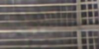
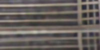
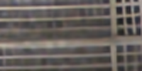
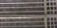
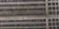
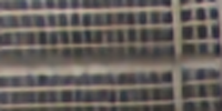
Urban100 ($4\times$): img_073 HR Bicubic EDSR [34] RCAN [78] RDN [79] IGNN [81] NLSA [81] IPT [5] SwinIR [33] SRFormer (ours)

Urban100 ($4\times$): img_092 HR Bicubic EDSR [34] RCAN [78] RDN [79] IGNN [81] NLSA [81] IPT [5] SwinIR [33] SRFormer (ours)

Figure 5: Qualitative comparison with recent state-of-the-art classical image SR methods on the $\times 4$ SR task.

Impact of kernel size of ConvFFN. We introduce ConvFFN in Sec. 3.2, which aims to encode more local information without increasing too many computations. In order to explore which kernel size can bring the best performance improvement, we attempt to use $3\times 3$ depth-wise convolution and $5\times 5$ depth-wise convolution and report the results in Table 2. Given that the depth-wise convolution has little effect on the number of parameters and MACs, we do not list them in the table. Obviously, $5\times 5$ depth-wise convolution leads to the best results. Thus, we use $5\times 5$ depth-wise convolution in our ConvFFN.

Large-window self-attention variants. In Sec. 3.3, we introduce another two large-window self-attention variants. We summarize the results in Table 3. Though token reduction can slightly improve SwinIR when using a large window, the number of parameters does not decrease and the performance gain is lower than ours. We argue that it is because directly applying downsampling operations to the key and value results in spatial information loss. For token sampling, the performance is even worse than the original SwinIR. We believe the reason is that dropping out some tokens severely breaks the image content structure.

	Method	Training Dataset	SET5 [3]		SET14 [70]		B100 [41]		Urban100 [18]		Manga109 [42]
			PSNR	SSIM	PSNR	SSIM	PSNR	SSIM	PSNR	SSIM	PSNR	SSIM
$\times 2$ SR	EDSR [34]	DIV2K	38.11	0.9602	33.92	0.9195	32.32	0.9013	32.93	0.9351	39.10	0.9773
	RCAN [78]	DIV2K	38.27	0.9614	34.12	0.9216	32.41	0.9027	33.34	0.9384	39.44	0.9786
	SAN [7]	DIV2K	38.31	0.9620	34.07	0.9213	32.42	0.9028	33.10	0.9370	39.32	0.9792
	IGNN [81]	DIV2K	38.24	0.9613	34.07	0.9217	32.41	0.9025	33.23	0.9383	39.35	0.9786
	HAN [45]	DIV2K	38.27	0.9614	34.16	0.9217	32.41	0.9027	33.35	0.9385	39.46	0.9785
	NLSA [43]	DIV2K	38.34	0.9618	34.08	0.9231	32.43	0.9027	33.42	0.9394	39.59	0.9789
	SwinIR [33]	DIV2K	38.35	0.9620	34.14	0.9227	32.44	0.9030	33.40	0.9393	39.60	0.9792
	ELAN [77]	DIV2K	38.36	0.9620	34.20	0.9228	32.45	0.9030	33.44	0.9391	39.62	0.9793
	SRFormer (ours)	DIV2K	38.45	0.9622	34.21	0.9236	32.51	0.9038	33.86	0.9426	39.69	0.9786
	IPT [5]	ImageNet	38.37	-	34.43	-	32.48	-	33.76	-	-	-
	SwinIR [33]	DF2K	38.42	0.9623	34.46	0.9250	32.53	0.9041	33.81	0.9427	39.92	0.9797
	EDT [31]	DF2K	38.45	0.9624	34.57	0.9258	32.52	0.9041	33.80	0.9425	39.93	0.9800
	SRFormer (ours)	DF2K	38.51	0.9627	34.44	0.9253	32.57	0.9046	34.09	0.9449	40.07	0.9802
	SRFormer+ (ours)	DF2K	38.58	0.9628	34.60	0.9262	32.61	0.9050	34.29	0.9457	40.19	0.9805
$\times 3$ SR	EDSR [34]	DIV2K	34.65	0.9280	30.52	0.8462	29.25	0.8093	28.80	0.8653	34.17	0.9476
	RCAN [78]	DIV2K	34.74	0.9299	30.65	0.8482	29.32	0.8111	29.09	0.8702	34.44	0.9499
	SAN [7]	DIV2K	34.75	0.9300	30.59	0.8476	29.33	0.8112	28.93	0.8671	34.30	0.9494
	IGNN [81]	DIV2K	34.72	0.9298	30.66	0.8484	29.31	0.8105	29.03	0.8696	34.39	0.9496
	HAN [45]	DIV2K	34.75	0.9299	30.67	0.8483	29.32	0.8110	29.10	0.8705	34.48	0.9500
	NLSA [43]	DIV2K	34.85	0.9306	30.70	0.8485	29.34	0.8117	29.25	0.8726	34.57	0.9508
	SwinIR [33]	DIV2K	34.89	0.9312	30.77	0.8503	29.37	0.8124	29.29	0.8744	34.74	0.9518
	ELAN [77]	DIV2K	34.90	0.9313	30.80	0.8504	29.38	0.8124	29.32	0.8745	34.73	0.9517
	SRFormer (ours)	DIV2K	34.94	0.9318	30.81	0.8518	29.41	0.8142	29.52	0.8786	34.78	0.9524
	IPT [5]	ImageNet	34.81	-	30.85	-	29.38	-	29.49	-	-	-
	SwinIR [33]	DF2K	34.97	0.9318	30.93	0.8534	29.46	0.8145	29.75	0.8826	35.12	0.9537
	EDT [31]	DF2K	34.97	0.9316	30.89	0.8527	29.44	0.8142	29.72	0.8814	35.13	0.9534
	SRFormer (ours)	DF2K	35.02	0.9323	30.94	0.8540	29.48	0.8156	30.04	0.8865	35.26	0.9543
	SRFormer+ (ours)	DF2K	35.08	0.9327	31.04	0.8551	29.53	0.8162	30.21	0.8884	35.45	0.9550
$\times 4$ SR	EDSR [34]	DIV2K	32.46	0.8968	28.80	0.7876	27.71	0.7420	26.64	0.8033	31.02	0.9148
	RCAN [78]	DIV2K	32.63	0.9002	28.87	0.7889	27.77	0.7436	26.82	0.8087	31.22	0.9173
	SAN [7]	DIV2K	32.64	0.9003	28.92	0.7888	27.78	0.7436	26.79	0.8068	31.18	0.9169
	IGNN [81]	DIV2K	32.57	0.8998	28.85	0.7891	27.77	0.7434	26.84	0.8090	31.28	0.9182
	HAN [45]	DIV2K	32.64	0.9002	28.90	0.7890	27.80	0.7442	26.85	0.8094	31.42	0.9177
	NLSA [43]	DIV2K	32.59	0.9000	28.87	0.7891	27.78	0.7444	26.96	0.8109	31.27	0.9184
	SwinIR [33]	DIV2K	32.72	0.9021	28.94	0.7914	27.83	0.7459	27.07	0.8164	31.67	0.9226
	ELAN [77]	DIV2K	32.75	0.9022	28.96	0.7914	27.83	0.7459	27.13	0.8167	31.68	0.9226
	SRFormer (ours)	DIV2K	32.81	0.9029	29.01	0.7919	27.85	0.7472	27.20	0.8189	31.75	0.9237
	IPT [5]	ImageNet	32.64	-	29.01	-	27.82	-	27.26	-	-	-
	SwinIR [33]	DF2K	32.92	0.9044	29.09	0.7950	27.92	0.7489	27.45	0.8254	32.03	0.9260
	EDT [31]	DF2K	32.82	0.9031	29.09	0.7939	27.91	0.7483	27.46	0.8246	32.03	0.9254
	SRFormer (ours)	DF2K	32.93	0.9041	29.08	0.7953	27.94	0.7502	27.68	0.8311	32.21	0.9271
	SRFormer+ (ours)	DF2K	33.09	0.9053	29.19	0.7965	28.00	0.7511	27.85	0.8338	32.44	0.9287

Table 4: Quantitative comparison of our SRFormer with recent state-of-the-art  classical image SR methods on five benchmark datasets. For a fair comparison, the parameters and MACs of SRFormer are lower than SwinIR (See supplementary material for details). The best performance is highlighted and the second is underlined.

	Method	Training Dataset	Params	MACs	SET5 [3]		SET14 [70]		B100 [41]		Urban100 [18]		Manga109 [42]
					PSNR	SSIM	PSNR	SSIM	PSNR	SSIM	PSNR	SSIM	PSNR	SSIM
$\times 2$ SR	EDSR-baseline [34]	DIV2K	1370K	316G	37.99	0.9604	33.57	0.9175	32.16	0.8994	31.98	0.9272	38.54	0.9769
	CARN [1]	DIV2K	1592K	222.8G	37.76	0.9590	33.52	0.9166	32.09	0.8978	31.92	0.9256	38.36	0.9765
	IMDN [19]	DIV2K	694K	158.8G	38.00	0.9605	33.63	0.9177	32.19	0.8996	32.17	0.9283	38.88	0.9774
	LAPAR-A [32]	DF2K	548K	171G	38.01	0.9605	33.62	0.9183	32.19	0.8999	32.10	0.9283	38.67	0.9772
	LatticeNet [40]	DIV2K	756K	169.5G	38.15	0.9610	33.78	0.9193	32.25	0.9005	32.43	0.9302	-	-
	ESRT [39]	DIV2K	751K	-	38.03	0.9600	33.75	0.9184	32.25	0.9001	32.58	0.9318	39.12	0.9774
	SwinIR-light [33]	DIV2K	910K	244G	38.14	0.9611	33.86	0.9206	32.31	0.9012	32.76	0.9340	39.12	0.9783
	ELAN [77]	DIV2K	621K	203G	38.17	0.9611	33.94	0.9207	32.30	0.9012	32.76	0.9340	39.11	0.9782
	SRFormer-light	DIV2K	853K	236G	38.23	0.9613	33.94	0.9209	32.36	0.9019	32.91	0.9353	39.28	0.9785
$\times 3$ SR	EDSR-baseline [34]	DIV2K	1555K	160G	34.37	0.9270	30.28	0.8417	29.09	0.8052	28.15	0.8527	33.45	0.9439
	CARN [1]	DIV2K	1592K	118.8G	34.29	0.9255	30.29	0.8407	29.06	0.8034	28.06	0.8493	33.50	0.9440
	IMDN [19]	DIV2K	703K	71.5G	34.36	0.9270	30.32	0.8417	29.09	0.8046	28.17	0.8519	33.61	0.9445
	LAPAR-A [32]	DF2K	594K	114G	34.36	0.9267	30.34	0.8421	29.11	0.8054	28.15	0.8523	33.51	0.9441
	LatticeNet [40]	DIV2K	765K	76.3G	34.53	0.9281	30.39	0.8424	29.15	0.8059	28.33	0.8538	-	-
	ESRT [39]	DIV2K	751K	-	34.42	0.9268	30.43	0.8433	29.15	0.8063	28.46	0.8574	33.95	0.9455
	SwinIR-light [33]	DIV2K	918K	111G	34.62	0.9289	30.54	0.8463	29.20	0.8082	28.66	0.8624	33.98	0.9478
	ELAN [77]	DIV2K	629K	90.1G	34.61	0.9288	30.55	0.8463	29.21	0.8081	28.69	0.8624	34.00	0.9478
	SRFormer-light	DIV2K	861K	105G	34.67	0.9296	30.57	0.8469	29.26	0.8099	28.81	0.8655	34.19	0.9489
$\times 4$ SR	EDSR-baseline [34]	DIV2K	1518K	114G	32.09	0.8938	28.58	0.7813	27.57	0.7357	26.04	0.7849	30.35	0.9067
	CARN [1]	DIV2K	1592K	90.9G	32.13	0.8937	28.60	0.7806	27.58	0.7349	26.07	0.7837	30.47	0.9084
	IMDN [19]	DIV2K	715K	40.9G	32.21	0.8948	28.58	0.7811	27.56	0.7353	26.04	0.7838	30.45	0.9075
	LAPAR-A [32]	DF2K	659K	94G	32.15	0.8944	28.61	0.7818	27.61	0.7366	26.14	0.7871	30.42	0.9074
	LatticeNet [40]	DIV2K	777K	43.6G	32.30	0.8962	28.68	0.7830	27.62	0.7367	26.25	0.7873	-	-
	ESRT [39]	DIV2K	751K	-	32.19	0.8947	28.69	0.7833	27.69	0.7379	26.39	0.7962	30.75	0.9100
	SwinIR-light [33]	DIV2K	930K	63.6G	32.44	0.8976	28.77	0.7858	27.69	0.7406	26.47	0.7980	30.92	0.9151
	ELAN [77]	DIV2K	640K	54.1G	32.43	0.8975	28.78	0.7858	27.69	0.7406	26.54	0.7982	30.92	0.9150
	SRFormer-light	DIV2K	873K	62.8G	32.51	0.8988	28.82	0.7872	27.73	0.7422	26.67	0.8032	31.17	0.9165

Table 5: Quantitative comparison of our SRFormer-light with recent state-of-the-art  lightweight image SR methods on five benchmark datasets. The best performance among all the model is highlighted.

4.3 Classical Image Super-Resolution

For the classical image SR task, we compare our SRFormer with a series of state-of-the-art CNN-based and Transformer-based SR methods: RCAN [78], RDN [79], SAN [7], IGNN [81], HAN [45], NLSA [43], IPT [5], SwinIR [33], EDT [31], and ELAN [77].

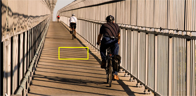
Urban100 ($4\times$): img_024 HR Bicubic CARN [1] IDN [20] IMDN [19] EDSR-baseline [34] LAPAR-A [32] LatticeNet [40] SwinIR-light [33] SRFormer-light (ours)

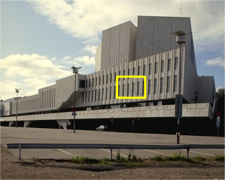
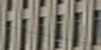
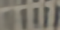
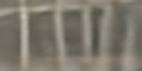
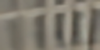
B100 ($4\times$): img_78004 HR Bicubic CARN [1] IDN [20] IMDN [19] EDSR-baseline [34] LAPAR-A [32] LatticeNet [40] SwinIR-light [33] SRFormer-light (ours)

Figure 6: Qualitative comparison of our SRFormer-light with recent state-of-the-art lightweight image SR methods for the $\times 4$ SR task. For each example, our SRFormer-light can restore the structures and details better than other methods.

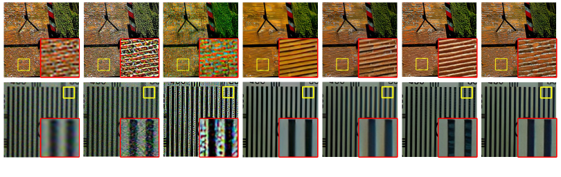
Figure 7: Qualitative comparisons with recent state-of-the-art methods on the $\times 4$ real-world image SR task.

Quantitative comparison. The quantitative comparison of the methods for classical image SR is shown in Table 4. For a fair comparison, the number of parameters and MACs of SRFormer are lower than SwinIR[33], see supplementary material for details. It can be clearly seen that SRFormer achieves the best performance on almost all five benchmark datasets for all scale factors. Since calculating self-attention within large windows can allow more information to be aggregated over a large area, our SRFormer performs much better on the high-resolution test set, such as Urban100 and Manga109. Especially, for the $\times 2$ SR training with DIV2K, our SRFormer achieves a 33.86dB PSNR score on the Urban100 dataset, which is 0.46dB higher than SwinIR but uses fewer parameters and computations. The performance boost gets even bigger when introducing ensemble strategy as SRFormer+. The above strongly supports that our SRFormer is effective and efficient.

Qualitative comparison. We show qualitative comparisons with other methods in Figure 5. From the first example of Figure 5, one can clearly observe that SRFormer can restore crisp and detailed textures and edges. In contrast, other models restore blurred or low-quality textures. For the second example, our SRFormer is the only model that clearly restores every letter. The qualitative comparison shows that our SRFormer can restore much better high-resolution images from the low-resolution ones.

4.4 Lightweight Image Super-Resolution

To demonstrate our model’s scalability and further proof of SRFormer’s efficiency and effectiveness, we train SRFormer-light and compare it with a list of state-of-the-art lightweight SR methods: EDSR-baseline [34], CARN [1], IMDN [19], LAPAR-A [32], LatticeNet [40], ESRT [39], SwinIR-light [33], and ELAN [77].

Quantitative comparison. The quantitative comparisons of lightweight image SR models are shown in Table 6. Following previous works [40, 1], we report the MACs by upscaling a low-resolution image to $1280\times 720$ resolution on all scales. We can see that our SRFormer-light achieves the best performance on all five benchmark datasets for all scale factors. Our model outperforms SwinIR-light [33] by up to $0.20$ dB PSNR scores on the Urban100 dataset and $0.25$ dB PSNR scores on the Manga109 dataset with even fewer parameters and MACs. The results indicate that despite the simplicity, our permuted self-attention is a more effective way to encode spatial information.

Qualitative comparison. We compare our SRFormer with state-of-the-art lightweight image SR models for qualitative comparisons in Figure 6. Notably, for all examples in Figure 6, SRFormer-light is the only model that can restore the main structures with less blurring and artifacts. This strongly demonstrates that the light version of SRFormer also performs better for restoring edges and textures compared to other methods.

4.5 Real-World Image Super-Resolution

Since the ultimate goal of image SR is to deal with rich real-world degradation and produce visually pleasing images, we follow SwinIR [33] to retrain our SRFormer by using the same degradation model as BSRGAN [74] and show results in Fig. 7. SRFormer still produces more realistic and visually pleasing textures without artifacts when facing with real-world images, which demonstrates the robustness of our method.

Figure 8: LAM results of SwinIR [33] and SRFormer on multiple challenging examples. We can see that SRFormer can perform SR reconstruction based on a particularly wide range of pixels.

4.6 LAM Comparison

To observe the range of utilized pixels for SR reconstruction, we compare our model with SwinIR using LAM [15] shown in Fig. 8. Based on the extremely large attention window, SRFormer infers SR images with a significantly wider range of pixels than SwinIR [33]. The experimental results are strongly consistent with our motivation and demonstrate the superiority of our method from the interpretability perspective.

5 Conclusion

In this paper, we propose PSA, an efficient self-attention mechanism which can efficiently build pairwise correlations within large windows. Based on our PSA, we design a simple yet effective Transformer-based model for single image super-resolution, called SRFormer. Due to the extremely large attention window and high-frequency information enhancement, SRFormer achieves state-of-the-art performance on classical, lightweight, and real-world SR task. We hope our permuted self-attention can be a paradigm of large window self-attention and serve as a useful tool for future research in super-resolution model design.

References

- [1] Namhyuk Ahn, Byungkon Kang, and Kyung-Ah Sohn. Fast, accurate, and lightweight super-resolution with cascading residual network. In ECCV, 2018.
- [2] Saeed Anwar, Salman Khan, and Nick Barnes. A deep journey into super-resolution: A survey. ACM Computing Surveys, 2020.
- [3] Marco Bevilacqua, Aline Roumy, Christine Guillemot, and Marie Line Alberi-Morel. Low-complexity single-image super-resolution based on nonnegative neighbor embedding. In BMVC, 2012.
- [4] Nicolas Carion, Francisco Massa, Gabriel Synnaeve, Nicolas Usunier, Alexander Kirillov, and Sergey Zagoruyko. End-to-end object detection with transformers. In ECCV, 2020.
- [5] Hanting Chen, Yunhe Wang, Tianyu Guo, Chang Xu, Yiping Deng, Zhenhua Liu, Siwei Ma, Chunjing Xu, Chao Xu, and Wen Gao. Pre-trained image processing transformer. In CVPR, 2021.
- [6] Xiangyu Chen, Xintao Wang, Jiantao Zhou, and Chao Dong. Activating more pixels in image super-resolution transformer. arXiv:2205.04437, 2022.
- [7] Tao Dai, Jianrui Cai, Yongbing Zhang, Shu-Tao Xia, and Lei Zhang. Second-order attention network for single image super-resolution. In CVPR, 2019.
- [8] Yingying Deng, Fan Tang, Weiming Dong, Chongyang Ma, Xingjia Pan, Lei Wang, and Changsheng Xu. Stytr2: Image style transfer with transformers. In CVPR, 2022.
- [9] Chao Dong, Chen Change Loy, Kaiming He, and Xiaoou Tang. Learning a deep convolutional network for image super-resolution. In ECCV, 2014.
- [10] Chao Dong, Chen Change Loy, and Xiaoou Tang. Accelerating the super-resolution convolutional neural network. In ECCV, 2016.
- [11] Alexey Dosovitskiy, Lucas Beyer, Alexander Kolesnikov, Dirk Weissenborn, Xiaohua Zhai, Thomas Unterthiner, Mostafa Dehghani, Matthias Minderer, Georg Heigold, Sylvain Gelly, et al. An image is worth 16x16 words: Transformers for image recognition at scale. In ICLR, 2020.
- [12] Yuxin Fang, Bencheng Liao, Xinggang Wang, Jiemin Fang, Jiyang Qi, Rui Wu, Jianwei Niu, and Wenyu Liu. You only look at one sequence: Rethinking transformer in vision through object detection. In NeurIPS, 2021.
- [13] Zhicheng Geng, Luming Liang, Tianyu Ding, and Ilya Zharkov. Rstt: Real-time spatial temporal transformer for space-time video super-resolution. In CVPR, 2022.
- [14] Ian J Goodfellow, Jean Pouget-Abadie, Mehdi Mirza, Bing Xu, David Warde-Farley, Sherjil Ozair, Aaron Courville, and Yoshua Bengio. Generative adversarial networks. arXiv:1406.2661, 2014.
- [15] Jinjin Gu and Chao Dong. Interpreting super-resolution networks with local attribution maps. In CVPR, 2021.
- [16] Chun-Le Guo, Qixin Yan, Saeed Anwar, Runmin Cong, Wenqi Ren, and Chongyi Li. Image dehazing transformer with transmission-aware 3d position embedding. In CVPR, 2022.
- [17] Muhammad Haris, Gregory Shakhnarovich, and Norimichi Ukita. Deep back-projection networks for super-resolution. In CVPR, 2018.
- [18] Jia-Bin Huang, Abhishek Singh, and Narendra Ahuja. Single image super-resolution from transformed self-exemplars. In CVPR, 2015.
- [19] Zheng Hui, Xinbo Gao, Yunchu Yang, and Xiumei Wang. Lightweight image super-resolution with information multi-distillation network. In ACM MM, 2019.
- [20] Zheng Hui, Xiumei Wang, and Xinbo Gao. Fast and accurate single image super-resolution via information distillation network. In CVPR, 2018.
- [21] Xiaozhong Ji, Yun Cao, Ying Tai, Chengjie Wang, Jilin Li, and Feiyue Huang. Real-world super-resolution via kernel estimation and noise injection. In CVPR Workshops, 2020.
- [22] Yifan Jiang, Shiyu Chang, and Zhangyang Wang. Transgan: Two transformers can make one strong gan. arXiv:2102.07074, 2021.
- [23] Younghyun Jo, Seoung Wug Oh, Jaeyeon Kang, and Seon Joo Kim. Deep video super-resolution network using dynamic upsampling filters without explicit motion compensation. In CVPR, 2018.
- [24] Jiwon Kim, Jung Kwon Lee, and Kyoung Mu Lee. Accurate image super-resolution using very deep convolutional networks. In CVPR, 2016.
- [25] Jiwon Kim, Jung Kwon Lee, and Kyoung Mu Lee. Deeply-recursive convolutional network for image super-resolution. In CVPR, 2016.
- [26] Diederik P Kingma and Jimmy Ba. Adam: A method for stochastic optimization. arXiv:1412.6980, 2014.
- [27] Wei-Sheng Lai, Jia-Bin Huang, Narendra Ahuja, and Ming-Hsuan Yang. Deep laplacian pyramid networks for fast and accurate super-resolution. In CVPR, 2017.
- [28] Christian Ledig, Lucas Theis, Ferenc Huszár, Jose Caballero, Andrew Cunningham, Alejandro Acosta, Andrew Aitken, Alykhan Tejani, Johannes Totz, Zehan Wang, et al. Photo-realistic single image super-resolution using a generative adversarial network. In CVPR, 2017.
- [29] Kwonjoon Lee, Huiwen Chang, Lu Jiang, Han Zhang, Zhuowen Tu, and Ce Liu. Vitgan: Training gans with vision transformers. arXiv:2107.04589, 2021.
- [30] Juncheng Li, Faming Fang, Kangfu Mei, and Guixu Zhang. Multi-scale residual network for image super-resolution. In ECCV, 2018.
- [31] Wenbo Li, Xin Lu, Jiangbo Lu, Xiangyu Zhang, and Jiaya Jia. On efficient transformer and image pre-training for low-level vision. arXiv:2112.10175, 2022.
- [32] Wenbo Li, Kun Zhou, Lu Qi, Nianjuan Jiang, Jiangbo Lu, and Jiaya Jia. Lapar: Linearly-assembled pixel-adaptive regression network for single image super-resolution and beyond. In NeurIPS, 2020.
- [33] Jingyun Liang, Jiezhang Cao, Guolei Sun, Kai Zhang, Luc Van Gool, and Radu Timofte. Swinir: Image restoration using swin transformer. In ICCV Workshops, 2021.
- [34] Bee Lim, Sanghyun Son, Heewon Kim, Seungjun Nah, and Kyoung Mu Lee. Enhanced deep residual networks for single image super-resolution. In CVPR Workshops, 2017.
- [35] Chengxu Liu, Huan Yang, Jianlong Fu, and Xueming Qian. Learning trajectory-aware transformer for video super-resolution. In CVPR, 2022.
- [36] Rui Liu, Hanming Deng, Yangyi Huang, Xiaoyu Shi, Lewei Lu, Wenxiu Sun, Xiaogang Wang, Jifeng Dai, and Hongsheng Li. Fuseformer: Fusing fine-grained information in transformers for video inpainting. In ICCV, 2021.
- [37] Ze Liu, Yutong Lin, Yue Cao, Han Hu, Yixuan Wei, Zheng Zhang, Stephen Lin, and Baining Guo. Swin transformer: Hierarchical vision transformer using shifted windows. In ICCV, 2021.
- [38] Liying Lu, Ruizheng Wu, Huaijia Lin, Jiangbo Lu, and Jiaya Jia. Video frame interpolation with transformer. In CVPR, 2022.
- [39] Zhisheng Lu, Hong Liu, Juncheng Li, and Linlin Zhang. Efficient transformer for single image super-resolution. arXiv:2108.11084, 2021.
- [40] Xiaotong Luo, Yuan Xie, Yulun Zhang, Yanyun Qu, Cuihua Li, and Yun Fu. Latticenet: Towards lightweight image super-resolution with lattice block. In ECCV, 2020.
- [41] David Martin, Charless Fowlkes, Doron Tal, and Jitendra Malik. A database of human segmented natural images and its application to evaluating segmentation algorithms and measuring ecological statistics. In ICCV, 2001.
- [42] Yusuke Matsui, Kota Ito, Yuji Aramaki, Azuma Fujimoto, Toru Ogawa, Toshihiko Yamasaki, and Kiyoharu Aizawa. Sketch-based manga retrieval using manga109 dataset. Multimedia Tools and Applications, 2017.
- [43] Yiqun Mei, Yuchen Fan, and Yuqian Zhou. Image super-resolution with non-local sparse attention. In CVPR, 2021.
- [44] Yiqun Mei, Yuchen Fan, Yuqian Zhou, Lichao Huang, Thomas S Huang, and Honghui Shi. Image super-resolution with cross-scale non-local attention and exhaustive self-exemplars mining. In CVPR, 2020.
- [45] Ben Niu, Weilei Wen, Wenqi Ren, Xiangde Zhang, Lianping Yang, Shuzhen Wang, Kaihao Zhang, Xiaochun Cao, and Haifeng Shen. Single image super-resolution via a holistic attention network. In ECCV, 2020.
- [46] Namuk Park and Songkuk Kim. How do vision transformers work? In ICLR, 2022.
- [47] Jingjing Ren, Qingqing Zheng, Yuanyuan Zhao, Xuemiao Xu, and Chen Li. Dlformer: Discrete latent transformer for video inpainting. In CVPR, 2022.
- [48] Wenzhe Shi, Jose Caballero, Ferenc Huszár, Johannes Totz, Andrew P Aitken, Rob Bishop, Daniel Rueckert, and Zehan Wang. Real-time single image and video super-resolution using an efficient sub-pixel convolutional neural network. In CVPR, 2016.
- [49] Robin Strudel, Ricardo Garcia, Ivan Laptev, and Cordelia Schmid. Segmenter: Transformer for semantic segmentation. In ICCV, 2021.
- [50] Zhiqing Sun, Shengcao Cao, Yiming Yang, and Kris M Kitani. Rethinking transformer-based set prediction for object detection. In ICCV, 2021.
- [51] Ying Tai, Jian Yang, and Xiaoming Liu. Image super-resolution via deep recursive residual network. In CVPR, 2017.
- [52] Ying Tai, Jian Yang, Xiaoming Liu, and Chunyan Xu. Memnet: A persistent memory network for image restoration. In ICCV, 2017.
- [53] Radu Timofte, Eirikur Agustsson, Luc Van Gool, Ming-Hsuan Yang, and Lei Zhang. Ntire 2017 challenge on single image super-resolution: Methods and results. In CVPR Workshops, 2017.
- [54] Tong Tong, Gen Li, Xiejie Liu, and Qinquan Gao. Image super-resolution using dense skip connections. In ICCV, 2017.
- [55] Hugo Touvron, Matthieu Cord, Matthijs Douze, Francisco Massa, Alexandre Sablayrolles, and Hervé Jégou. Training data-efficient image transformers & distillation through attention. arXiv:2012.12877, 2020.
- [56] Hugo Touvron, Matthieu Cord, Alexandre Sablayrolles, Gabriel Synnaeve, and Hervé Jégou. Going deeper with image transformers. In ICCV, 2021.
- [57] Peihao Wang, Wenqing Zheng, Tianlong Chen, and Zhangyang Wang. Anti-oversmoothing in deep vision transformers via the fourier domain analysis: From theory to practice. arXiv:2203.05962, 2022.
- [58] Wenhai Wang, Enze Xie, Xiang Li, Deng-Ping Fan, Kaitao Song, Ding Liang, Tong Lu, Ping Luo, and Ling Shao. Pyramid vision transformer: A versatile backbone for dense prediction without convolutions. In ICCV, 2021.
- [59] Xintao Wang, Kelvin CK Chan, Ke Yu, Chao Dong, and Chen Change Loy. Edvr: Video restoration with enhanced deformable convolutional networks. In CVPR Workshops, 2019.
- [60] Xiaolong Wang, Ross Girshick, Abhinav Gupta, and Kaiming He. Non-local neural networks. In CVPR, 2018.
- [61] Xintao Wang, Liangbin Xie, Chao Dong, and Ying Shan. Real-esrgan: Training real-world blind super-resolution with pure synthetic data. In ICCV, 2021.
- [62] Xintao Wang, Ke Yu, Chao Dong, and Chen Change Loy. Recovering realistic texture in image super-resolution by deep spatial feature transform. In CVPR, 2018.
- [63] Xintao Wang, Ke Yu, Shixiang Wu, Jinjin Gu, Yihao Liu, Chao Dong, Yu Qiao, and Chen Change Loy. Esrgan: Enhanced super-resolution generative adversarial networks. In ECCV Workshops, 2018.
- [64] Zhendong Wang, Xiaodong Cun, Jianmin Bao, Wengang Zhou, Jianzhuang Liu, and Houqiang Li. Uformer: A general u-shaped transformer for image restoration. In CVPR, 2022.
- [65] Enze Xie, Wenhai Wang, Zhiding Yu, Anima Anandkumar, Jose M Alvarez, and Ping Luo. Segformer: Simple and efficient design for semantic segmentation with transformers. In NeurIPS, 2021.
- [66] Yue Yang and Yong Qi. Image super-resolution via channel attention and spatial graph convolutional network. Pattern Recognition, 2021.
- [67] Li Yuan, Yunpeng Chen, Tao Wang, Weihao Yu, Yujun Shi, Zi-Hang Jiang, Francis E.H. Tay, Jiashi Feng, and Shuicheng Yan. Tokens-to-token vit: Training vision transformers from scratch on imagenet. In ICCV, 2021.
- [68] Li Yuan, Qibin Hou, Zihang Jiang, Jiashi Feng, and Shuicheng Yan. Volo: Vision outlooker for visual recognition. TPAMI, 2022.
- [69] Syed Waqas Zamir, Aditya Arora, Salman Khan, Munawar Hayat, Fahad Shahbaz Khan, and Ming-Hsuan Yang. Restormer: Efficient transformer for high-resolution image restoration. In CVPR, 2022.
- [70] Roman Zeyde, Michael Elad, and Matan Protter. On single image scale-up using sparse-representations. In Curves and Surfaces, 2010.
- [71] Bowen Zhang, Shuyang Gu, Bo Zhang, Jianmin Bao, Dong Chen, Fang Wen, Yong Wang, and Baining Guo. Styleswin: Transformer-based gan for high-resolution image generation. In CVPR, 2022.
- [72] Dafeng Zhang, Feiyu Huang, Shizhuo Liu, Xiaobing Wang, and Zhezhu Jin. Swinfir: Revisiting the swinir with fast fourier convolution and improved training for image super-resolution. arXiv:2208.11247, 2022.
- [73] Kai Zhang, Yawei Li, Wangmeng Zuo, Lei Zhang, Luc Van Gool, and Radu Timofte. Plug-and-play image restoration with deep denoiser prior. TPAMI, 2021.
- [74] Kai Zhang, Jingyun Liang, Luc Van Gool, and Radu Timofte. Designing a practical degradation model for deep blind image super-resolution. In ICCV, 2021.
- [75] Kai Zhang, Wangmeng Zuo, and Lei Zhang. Learning a single convolutional super-resolution network for multiple degradations. In CVPR, 2018.
- [76] Wenlong Zhang, Yihao Liu, Chao Dong, and Yu Qiao. Ranksrgan: Generative adversarial networks with ranker for image super-resolution. In ICCV, 2019.
- [77] Xindong Zhang, Hui Zeng, Shi Guo, and Lei Zhang. Efficient long-range attention network for image super-resolution. arXiv:2203.06697, 2022.
- [78] Yulun Zhang, Kunpeng Li, Kai Li, Lichen Wang, Bineng Zhong, and Yun Fu. Image super-resolution using very deep residual channel attention networks. In ECCV, 2018.
- [79] Yulun Zhang, Yapeng Tian, Yu Kong, Bineng Zhong, and Yun Fu. Residual dense network for image super-resolution. In CVPR, 2018.
- [80] Sixiao Zheng, Jiachen Lu, Hengshuang Zhao, Xiatian Zhu, Zekun Luo, Yabiao Wang, Yanwei Fu, Jianfeng Feng, Tao Xiang, Philip HS Torr, et al. Rethinking semantic segmentation from a sequence-to-sequence perspective with transformers. In CVPR, 2021.
- [81] Shangchen Zhou, Jiawei Zhang, Wangmeng Zuo, and Chen Change Loy. Cross-scale internal graph neural network for image super-resolution. In NeurIPS, 2020.