Econotaxis in modeling urbanization by labor force migration

Abstract

Individual participants in human society collectively exhibit aggregation behavior. In this study, we present a simple microscopic model of labor force migration by employing the active Brownian particles framework. Through agent-based simulations, we find that our model produces clusters of agents from a random initial distribution. Furthermore, two empirical regularities called Zipf’s and Okun’s laws were observed in our model. To reveal the mechanism underlying the reproduced agglomeration phenomena, we derived an extended Keller–Segel system, a classic model that describes the aggregation behavior of biological organisms called taxis, from our microscopic model. The obtained macroscopic system indicates that the agglomeration of the workforce in real world can be accounted for through a new type of taxis central to human behavior, which highlights the relevance of urbanization to blow-up phenomena in the derived PDE system. We term it “econotaxis.”

I Introduction

Urbanization, a process of population concentration Tisdale (1941), is recognized as a significant characteristic of human society Berry (2008); Boddy (1999); Ottaviano and Thisse (2004). Having occurred for more than three hundred years, urbanization continues, showing an increasing tendency toward agglomeration Tisdale (1941); Fujita and Thisse (2002). The topic has been discussed in many fields, including geography, economics, and urban planning, from a wide range of perspectives. Nevertheless, the manner in which people and firms get concentrated is expected to be widely universal, given that similar agglomeration patterns and hierarchical structures have been discovered across the globe Fujita and Thisse (1996); Brakman and Garretsen (2003); Berry (2008).

In the last two centuries, theories have been proposed to explain the spatial distributions of human activity and settlements, such as von Thünen’s theory Grotewold (1959); Mäki (2004), Weberian location theory Isard (1949); Capello (2014), and the central place theory King (2020); Mulligan (1984). Toward the end of last century, in economics, a new discipline called New Economic Geography was established, and spatial economic problems were beginning to be considered seriously Ottaviano and Thisse (2004); Martin (1999). Currently, these problems are commonly addressed by regarding them as either a cost-minimization (or profit-maximization) problem or an equilibrium state where the benefits of agglomeration and the resulting costs balance each other Glaeser (2010); Puga (2010); Duranton and Puga (2004); Boddy (1999); Ottaviano and Thisse (2004).

However, theories proposed in previous studies have not led to a a clear understanding of agglomeration phenomena Berry (2008); Fujita and Thisse (1996). For example, some of them have been criticized for their unestablished empirical basis, unclear microscopic underpinnings, lack of circular causation, little reference to intraregional dynamics and emergent nature of urban areas King (2020); Tisdale (1941); Martin (1999); Boddy (1999); Krugman (1992). Furthermore, theoretical arguments derived from these theories are not always verifiable Duranton and Puga (2004); Martin (1999) because they have often been formulated in an oversimplified manner or under implausible assumptions, thereby making a comparison with empirical data unfeasible Scott (2006). Thus, a new yet simple model that aligns with empirical observations is required to uncover the fundamental mechanism driving agglomeration in human society.

Over the past few decades, statistical physics has proven to be a powerful tool for examining and understanding social dynamics Castellano et al. (2009). A central example is human mobility patterns, an emerging field attributed to the increasing availability of large-scale empirical data Gonzalez et al. (2008); Schläpfer et al. (2021); Shida et al. (2020). Although most of them focus on human mobility in the relatively short run, migration patterns over centuries, such as urbanization, can be studied similarly.

Consistent with this line of research, the author in Schweitzer (2002) prominently introduced a dynamic model of economic agglomeration by employing active Brownian particles (ABPs) Schweitzer (2003); Romanczuk et al. (2012), the concept of which was originally introduced in Schimansky-Geier et al. (1995). ABPs (or sometimes Brownian agents Helbing (2001)) are Brownian particles capable of generating a field that, in turn, influences their motion Romanczuk et al. (2012). Using this framework, the author investigated the emergence and evolution of economic centers and observed their coexistence. However, a major drawback of this approach is that the reproduced emergence of central regions is attributable to the presupposed strong nonlinearity of a production function, coupled with a rapid response of the local employment status to changes in local economic circumstances.

More specifically, in Schweitzer (2002), two types of agents, employed and unemployed, that transition between one another are considered, and only the unemployed ones can migrate in a two-dimensional domain. They, as Brownian agents, navigate the domain according to the following deterministic force $f(r)$:

$$f(r) =\nabla\omega(r),\quad\omega(r)=\frac{\delta Y}{\delta l}(l(r)),$$

$$Y(l) \propto[A_{0}+\exp(a_{1}l-a_{2}l^{2})]\,l^{\beta},$$ (1)

where $r$ represents position, $\omega(r)$ a wage field, $Y(l)$ production output as a function of labor, $l(r)$ the density of employed agents, and $A_{0},a_{1},a_{2},\beta$ are some positive constants. The issue with this formulation is that the initiated agglomeration depends entirely on the artificial modification, which is expressed as an exponential term in Eq. (1), of a normal production function. Consequently, $f$ works on unemployed agents as an agglomeration force only in a certain middle range of $l$. Therefore, agglomeration cannot arise from a random initial distribution of employed agents unless $l$ is initially set high enough. Nonetheless, agglomeration does occur in Schweitzer (2002) because another type of strong nonlinearity is assumed in the rates of transition between two states (employed and unemployed) to help $l$ increase and reach that “special” range. In other words, without these technical conditions, city-like regions would not appear, let alone their coexistence. Therefore, the aforementioned formulation may not be successful in providing plausible explanations for real-world agglomeration phenomena such as urbanization.

As with the tendency toward agglomeration, society is endowed with other characteristic features, many of which have been presented in the form of statistical regularities. The rank-size rule is a power-law relationship between the city size and its rank in a given urban system Hinloopen and van Marrewijk (2006); Fujita and Thisse (1996); Rose (2005), described in the following mathematical form:

$$(\text{city size})\propto(\text{rank})^{-\gamma},$$ (2)

where the rank-size exponent $\gamma$ is close to 1 Gabaix and Ioannides (2004); Veneri (2016). This provides a good rule of thumb that the $N$th largest city has a population proportional to one-$N$th the population of the largest city in a community, which is also known as a good approximation of Zipf’s law Reed (2002); Gabaix (1999). Zipf’s law holds only for large cities Hinloopen and van Marrewijk (2006). The well-documented regularity is generally considered a manifestation of universality in human migration and settlements. Several models have been proposed to replicate the law, such as Steindl’s and Simon’s models Simon (1955); Gabaix (1999). However, they have been criticized for their counterfactual settings or limited applicability.

In relation to agglomeration phenomena, empirical studies have indicated that a rank-size distribution demonstrating Zipf’s law is a sign of urban development Cristelli et al. (2012); Wang and Chen (2021); Guérin-Pace (1995). Several studies have reported a gradual yet continuing increase in rank-size exponents even after they reach $1$ , such as the city-size distribution in China from 1982 to 2010 Wang and Chen (2021) and the country-size distribution of the 50 largest countries worldwide from 1990 to 2050 (projections included) Rose (2005). As seen previously, this regularity appears on extensive and dynamic scales, thus requiring a more comprehensive theory of the law Rose (2005).

Okun’s law is another statistical characteristic studied in a large body of macroeconomics literature Okun (1963). It refers to the negative correlation between output growth and changes in the unemployment rate during an interval(e.g., quarterly) Lee (2000). That is, positive output growth corresponds to a decreasing unemployment rate. For empirical testing, the law can be expressed as follows Knotek II (2007):

$$\frac{\Delta Y_{tot}}{Y_{tot}}\approx-c\,\Delta\mu,$$ (3)

where $Y_{tot}$ is the total output across a nation, and $\mu$ is the (national) average unemployment rate at a given time. $\Delta Y_{tot}$ and $\Delta\mu$ represent changes in the respective variables during a given interval. In the case of the U.S. economy, it predicts approximately a 2for every one-point decrease in the unemployment rate, which translates to $c\approx 2$ Lee (2000); Cuaresma (2003). An accumulated body of empirical and theoretical research has demonstrated that the law, including the coefficient, appears robust to some extent over different periods and under different methods of analysis Ball et al. (2013). Although there has been some variability in the coefficient among countries and controversy regarding the reliability of the law, the relationship is typical of most economies Lee (2000). Many existing theories consider fluctuations from hypothetical baseline values of certain variables that are not directly observable yet fail to account for empirically observed coefficients Ball et al. (2013). Therefore, a new, unified theoretical approach may be of benefit Knotek II (2007).

To address the aforementioned issues, we propose a simple labor migration model and show through agent-based simulation (ABS) that the model initiates the aggregation of agents from a random initial distribution. We then demonstrate that the obtained spatiotemporal population distribution and economic circumstances are quantitatively similar to those in the real world simply by investigating the reproduced dynamics in terms of Zipf’s and Okun’s laws, respectively. To the best of our knowledge, an attempt to reproduce these two empirical laws in a single model of urbanization has never been made. Our ultimate goal is to detect the key elements of agglomeration phenomena in human society and reveal the fundamental mechanism underlying them.

The paper is organized as follows: In Sec. II, we develop a model of urbanization using ABPs and delineate our simulation scheme. In Sec. III, we provide simulation results and derive a corresponding macroscopic model. Next, we highlight its relevance to the classical Keller–Segel model (a classic model that describes the aggregation behavior of biological organisms called taxis) and introduce a key concept called econotaxis to characterize the reproduced aggregation phenomena. Lastly, in Sec. IV, we summarize our main results and discuss them from the perspective of some potential relevance to future work.

II Methods

II.1 Mathematical Model

We introduce a stochastic model of labor migration, following the framework proposed in Schweitzer (2002). Let us consider $N$ identical Brownian agents that migrate in a domain $\Omega=[0,L]^{2}\subset\mathbb{R}^{2}$, with $L$ being the system size. Brownian agents are characterized by their internal states $\theta_{i}$ and positions $r_{i}\in\Omega\,(i=1,\cdots,N)$, and they interact indirectly with each other via their external environment Schweitzer (2003); Castellano et al. (2009). Each agent is assigned either the employed ($\theta_{i}=0$) or unemployed ($\theta_{i}=1$) status, and their spatial movements are governed by either of the following Langevin equations depending on their current states:

$$\dot{r_{i}} =\sqrt{2D_{l}}\,\xi_{i}(t)\quad(\theta_{i}=0),$$ (4)

$$\dot{r_{i}} =\sqrt{2D_{n}}\,\xi_{i}(t)+F(t)\quad(\theta_{i}=1),$$ (5)

where $\xi_{i}(t)$ represents white Gaussian noise with zero mean and $\left<{\xi_{i}(t)\cdot\xi_{j}(t^{\prime})}\right>=\delta_{i,j}\delta(t-t^{\prime})$. $D_{n}$ and $D_{l}$ are some constants satisfying $D_{n}\gg D_{l}$. This implies that employed agents are almost intrinsically immobile compared to the unemployed because people in employment reasonably prefer stability in their lives and are thus less motivated to migrate than the unemployed ones, who have incentives to travel even long distances to obtain a job. We also suppose that agents transition their status from $\theta_{i}=0$ to $\theta_{i}=1$ with a transition probability $k^{-}$, and vice versa with $k^{+}$.

Now, we are left with the determination of $F(t)$, which plays a significant role in the spatiotemporal dynamics of population distribution. Unlike Schweitzer (2002), we assume that unemployed agents prefer economically active places. In this context, we mean unemployed agents tend to migrate toward areas where a large economic output is produced. In other words, unemployed agents are drawn to places where, for example, well-paid or secure jobs are available, and their chances of being provided with those opportunities improve as the local economic production increases. Although living in those places can be accompanied, in reality, by various issues such as higher living costs and crime rates, we postulate that they offer significant benefits in almost every aspect of one’s life, and the benefits of dwelling in urban areas generally outweigh the disadvantages. Empirical evidence seems to support this argument Berry (2008); Boddy (1999). Studies have shown that poorer people are attracted to cities, that urban-ward migration is a response to growing economic opportunity, and that a positive relationship exists between wages and city size. In economics, production output can be computed as a function of the number of workers. The simplest and the most commonly used form is the Cobb–Douglass production function Fujita and Thisse , in which output is assumed to increase in proportion to the number of workers raised to some power. In our model, all of the above ansatzes can be summarized in the following equations:

$$f(r)=\alpha\nabla\ln[Y(l(r))+1],$$ (6)

$$Y(l)=A\,l^{\beta},$$ (7)

where $f(r)$ is a deterministic force exerted on the agents located at $r$, $l(r)$ is the density of employed agents, $\alpha$ and $A$ are some constants, $Y(l)$ is a production function, and $\beta$ is a positive exponent smaller than $1$. The condition $\beta<1$ ensures decreasing returns to scale, which refers to situations where increasing input by a factor of $\eta$ results in increasing the output by a factor less than $\eta$ Fujita and Thisse . The logarithm in Eq. (6) is based on Fechner’s law, originally proposed in psychophysics, which states that sensation grows proportional to stimulus intensity Nutter Jr (2010). Specifically, we regard production output as a perceivable stimulus to which unemployed agents respond in search of better employment opportunities. Note that we assume no strong nonlinearity in Eqs. (6) and (7), as opposed to Schweitzer (2002).

With regard to Eq. (5), to specify $F$, we first consider a spatial discretization of the entire domain $\Omega$ into square boxes with a unit length $h$, each of which is denoted by $\Lambda_{mn}$, with $m$ and $n$ denoting spatial indices. Notice that a unique $\Lambda_{mn}\subset\Omega$ exists for any given $r_{i}(t)$ such that $r_{i}(t)\in\Lambda_{mn}$. We define $F(t)$ by

$$F(t)$$

$$=\frac{1}{2h}\begin{pmatrix}(\ln[Y(l_{m+1,n})+1]-\ln[Y(l_{m-1,n})+1])\\ (\ln[Y(l_{m,n+1})+1]-\ln[Y(l_{m,n-1})+1])\end{pmatrix},$$ (8)

$$l_{m,n}(t)=\frac{1}{h^{2}}\sum_{j=1}^{N}\mathds{1}_{\Lambda_{mn}}(r_{j}(t))\delta_{\theta_{j}(t),0},$$ (9)

where $\mathds{1}_{I}(x)=1\;(x\in I);\,0\;(x\notin I)$. Note that $F$ in Eq. (8) plays the same role as $f$ in Eq. (6), except that it is reinvented for ABS using the central difference method. Practically, $\{l_{m,n}(t)\}_{m,n}$ is equivalent to a uniformly binned histogram that represents the spatial distribution of employed agents.

II.2 Simulation Scheme

We used the Euler–Maruyama method for time discretization of Eqs. (4) and (5) with an interval of length $1$. The transition between the two statuses (employed and unemployed) was also implemented during each time step. All agents update their positions and status simultaneously, which constitutes a unit time step, and this entire updating process was iterated throughout the simulation. We performed our simulations with periodic boundary conditions.

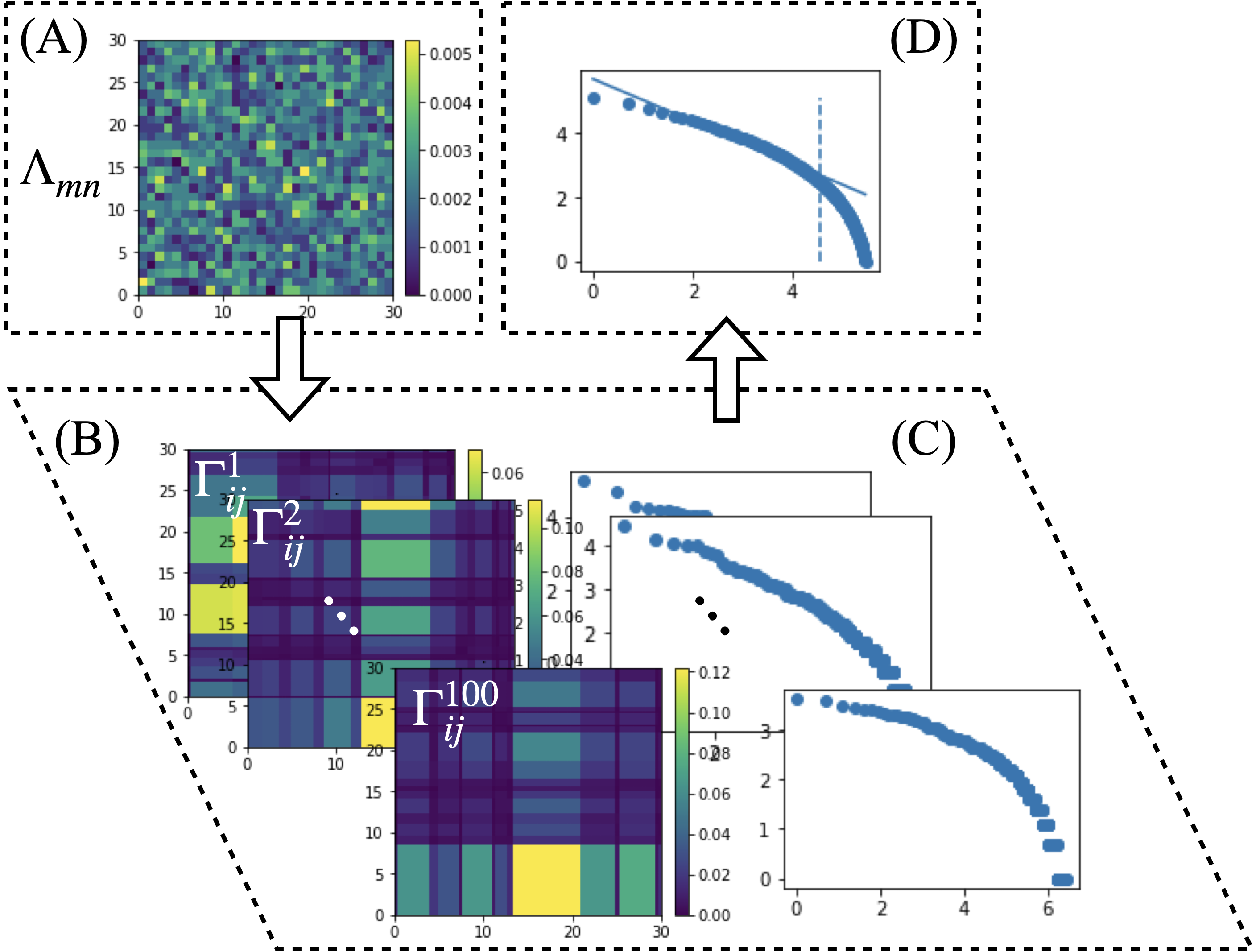
Our model was also investigated in terms of two empirical laws. First, we clarified the definition of a city in the simulation to produce rank-size distributions. Unsurprisingly, what defines a city is debatable Gabaix and Ioannides (2004). Here we adopted a simple approach, in which we equated cities with the entire region divided into smaller rectangular areas using a non-uniform spatial grid. More specifically, we separated the domain $\Omega$ into smaller rectangles by applying a coarse non-uniform spatial grid, which we represented by $\{\Gamma_{ij}\}$, having a fixed number of straight lines on each side with their intervals randomly specified. We then determined each rectangular area defined by the non-uniform grid as an equivalent of a city. Furthermore, to mitigate the stochastic influence of the aforementioned arrangement of cities on the resulting rank-size distributions, we “filtered” the same spatial population distribution produced via ABS by a hundred different non-uniform grids, $\{\Gamma^{k}_{ij}\}_{i,j}(k=1,\cdots,100)$, and obtained a mean rank-size distribution following the same procedure using the grids (see Fig. 1). The average size of a city must be effectively larger than the unit spatial length $h$, such that, the scaling relationship between the migration of agents and the average city size is not violated. In summary, the grid $\{\Gamma^{k}_{ij}\}_{i,j}$ is non-uniform, generated many times, and coarse compared to $\{\Lambda_{mn}\}_{m,n}$, which is a fine uniform grid with a unit length $h$, used only for computing our agent-based model.

Figure 1: Schematic view of computing a mean rank-size distribution by applying different arrangements of cities. (A) An agent-based simulation is implemented using the fine uniform grid $\{\Lambda_{mn}\}$. (B) The entire region is randomly divided into rectangles 100 times using coarse, non-uniform grids $\{\Gamma^{k}_{ij}\}_{i,j}$. (C) Rank-size distributions are produced based on different configurations of cities corresponding to the coarse, non-uniform grids $\{\Gamma_{ij}^{k}\}_{i,j}$. (D) A mean rank-size distribution is obtained that is averaged over all rank-size distributions produced in (C). In the following simulations, we prepare 289 cities in the $30\times 30$ field ($L=30,h=1$) by applying a hundred $17\times 17$ non-uniform grids generated randomly.

Regarding Okun’s law, we investigate whether fractional changes in the total output, $\Delta Y_{tot}/Y_{tot}$, are (anti-)correlated with contemporaneous changes in the overall unemployment rate, $\Delta\mu$. Note that $Y_{tot}(t)=\sum_{m,n}Y(l_{m,n}(t))$ and $\mu(t)=\left(\sum_{i=1}^{N}\delta_{\theta_{i}(t),1}\right)/N$ in our model. We investigate the relationship at every time step.

III Results

III.1 Aggregation phenomena

Figure 2: Snapshots demonstrating the aggregation of agents produced by ABS. The parameters are as follows: $N=4000,D_{n}=0.30,D_{l}=0.03,A=1,\beta=0.67,k^{+}=0.30,k^{-}=0.55$. This set of parameters applies to the results in all figures that follow unless otherwise noted. The colored bars display the fractions of employed (left) and unemployed (right) agents in a uniformly discretized box relative to the total number of agents in each respective employment status at the time presented.

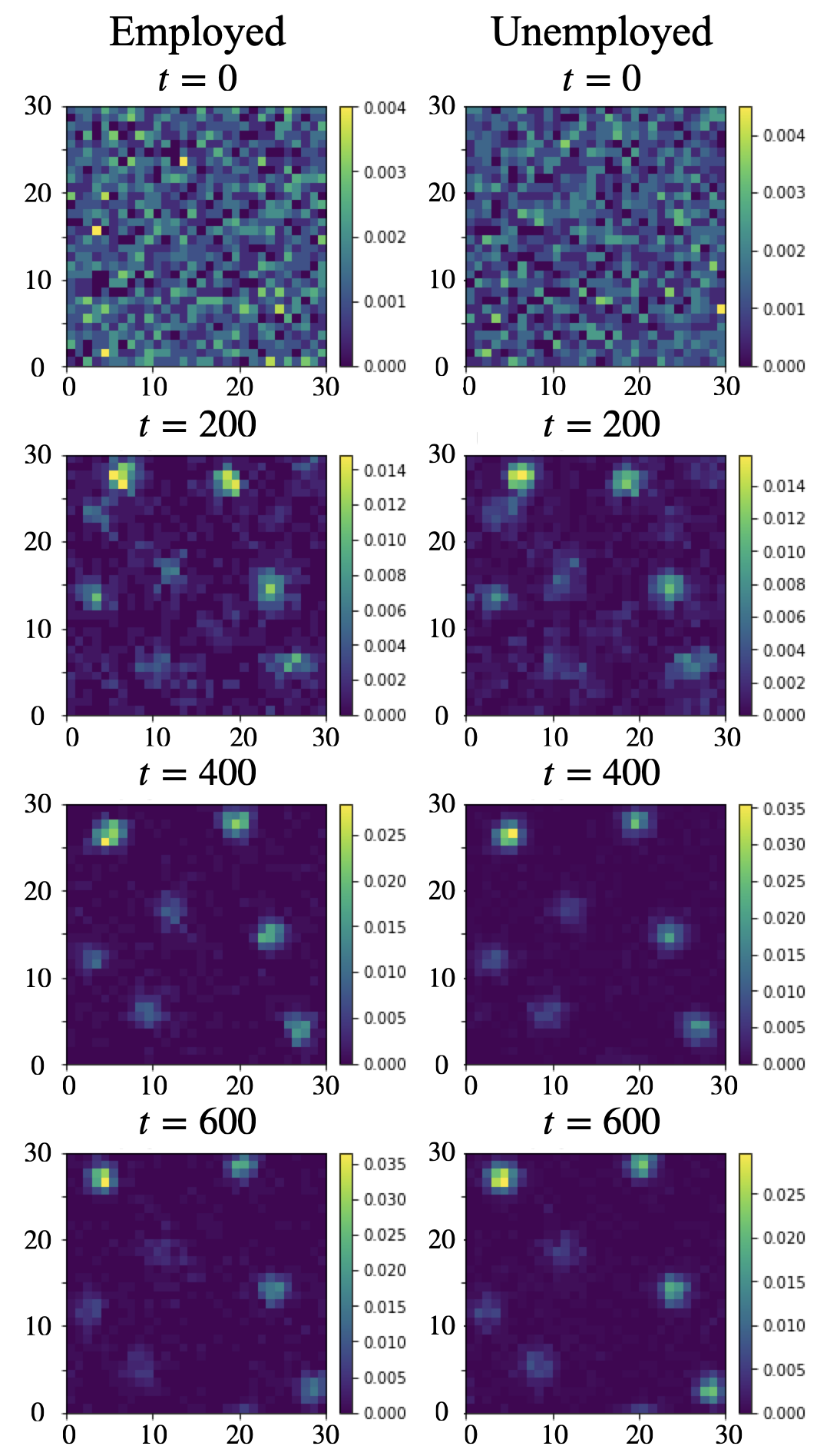
Based on the method described in Sec.II.2, we implemented ABS to investigate the behavior of our model, focusing primarily on the spatiotemporal dynamics of the agent distributions. Fig. 2 shows an evolution of the spatial distributions of employed and unemployed agents, illustrating the manner in which they undergo the process of self-organization from a spatially disordered to an ordered state. Distributed randomly at the initial stage, these agents separate into aggregations before $t=200$. Later, the clusters become tighter, and only some continue to intensify in magnitude while others disappear (from $t=400$ to $t=600$). In the following, we will discuss the mechanism of the observed aggregation phenomena.

In Eq. (5), two opposing forces compete with one another – agglomeration and dispersion forces. An agglomeration force arises from the differences in economic circumstances between neighboring places, resulting from the differences in the number of people hired at these places (see Eqs. (8) and (9)). Meanwhile, a dispersion force is caused by random fluctuations in the motion of agents. If agglomeration overrides dispersion, unemployed agents start forming clusters. Once this occurs, the effect amplifies: the more unemployed agents there are, the more employed agents there will be because they constantly transition their employment status from unemployed to employed and vice versa. This leads to a higher production output, which results in even stronger agglomeration forces. This positive feedback allows for the emergence of disproportionately highly populated areas. In Eq. (4), in contrast, only a dispersion force is at play. Thus, aggregation of employed agents is caused solely by clustered unemployed agents transitioning their job status.

Figure 3: Snapshots produced by ABS in which no aggregation occurs owing to a significant imbalance of transition rates. The parameters are the same as those in Fig. 2, except that the transition rates are chosen as $k^{+}=0.9,k^{-}=0.1$ at the top and $k^{+}=0.1,k^{-}=0.9$ at the bottom.

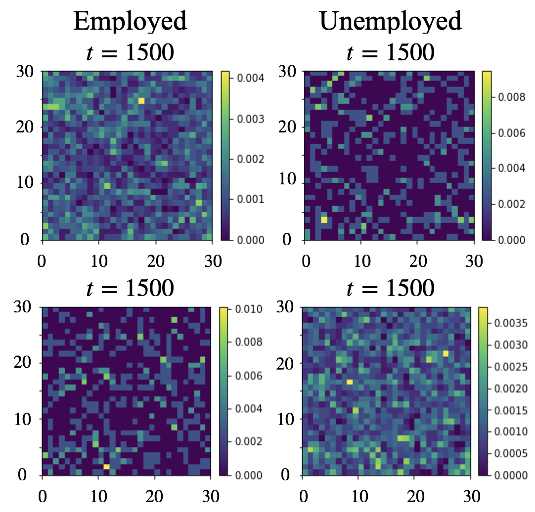
Regarding the transitions of employment status, the balance between transition probabilities can be a critical factor in determining whether agents end up in aggregations. According to our simulations, agents seem to be prevented from being aggregated when either of the transition probabilities is significantly larger than the other (Fig. 3). We speculate that this is because a lopsided pair of transition probabilities produces a disproportionately large number of agents of one type and a few of the others, as the balance $k^{+}/k^{-}$ fundamentally determines both the overall and local employment rates. If most agents are employed, the population distribution becomes flat faster than some places gain momentum to grow at the expense of others. If most agents are unemployed, however, few employed agents are available to ramp up local production, which weakens the agglomeration force enough to stop causing particular orientation in the movements of unemployed agents. Therefore, keeping the ratio close to one is necessary to set off aggregation phenomena in the model.

III.2 Empirical laws

Figure 4: Evolution of the mean rank-size distribution for the data presented in Fig. 2. The data are presented in blue circles. The blue-shaded areas represent the standard deviations caused by applying a hundred different city configurations. The fitting interval is truncated at the 75th percentile (i.e., the top $25\%$), as indicated by the dotted vertical line. The truncated distribution is regressed linearly (black dashed line) using the ordinary least squares (OLS) method.

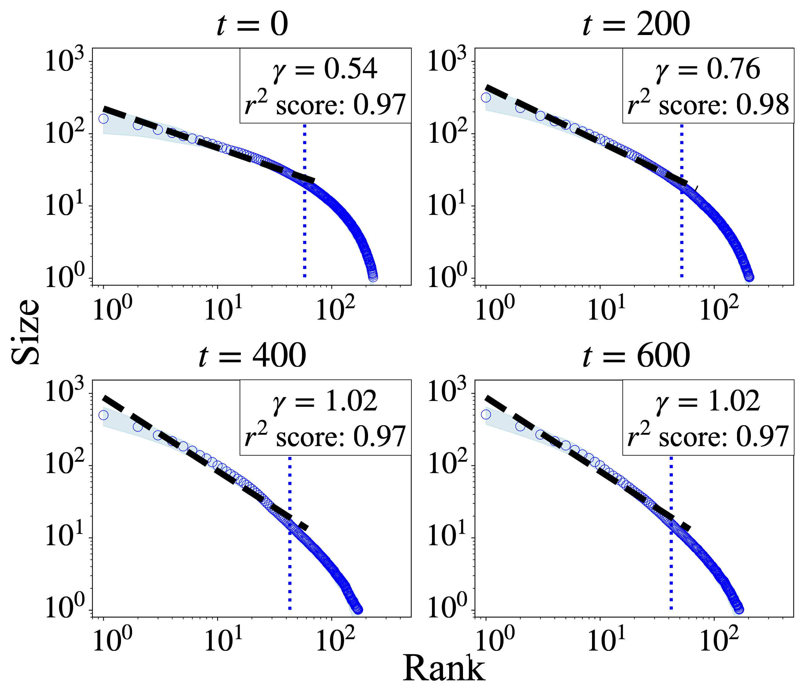
Now that our model reproduces aggregation phenomena, we investigate how rank-size distributions evolve as well as their relevance to Zipf’s law (Fig. 4). Note that none of the rectangular areas with a population of zero or one are considered cities in the first place, either in the data of Fig. 4 or in the following discussion. First, high-ranking cities (above the $75$th percentile) appear to fit well with a straight line at all times presented in the figure on a logarithmic scale. Notably, as time progresses, the slope becomes steeper, and the exponent (i.e., $\gamma$ in Eq. (2)) gradually approaches $1$ (the Zipf exponent) without sacrificing the $r^{2}$ values and then stabilizes around (from $t=400$ to $t=600$). In other words, the city size distribution exhibits Zipf’s law corresponding to the process of aggregation.

Furthermore, the standard deviation (owing to how we arrange cities) remains small at all ranks and at all times presented. Although, during an initial stage, the aforementioned method causes moderately large fluctuations in the sizes of high-ranking cities, these fluctuations gradually disappear as the agents form clusters (see Figs. 2 and 4). In empirical studies, the law has been shown to apply to data from various countries despite their varying definitions of an administrative city Veneri (2016). The small fluctuations shown in Fig. 4 by the shading may suggest a similar type of robustness of the system for different units of analysis.

Figure 5: Time series of the rank-size exponent in Fig. 4 for an extended time window. The $r^{2}$ score is above $0.96$ at all $t$. The period when Zipf’s exponent appears to be stable (from $t\approx 350$ to $800$) suggests that the system is in a metastable state. Only fluctuations that are large enough can bring the system out of this state.

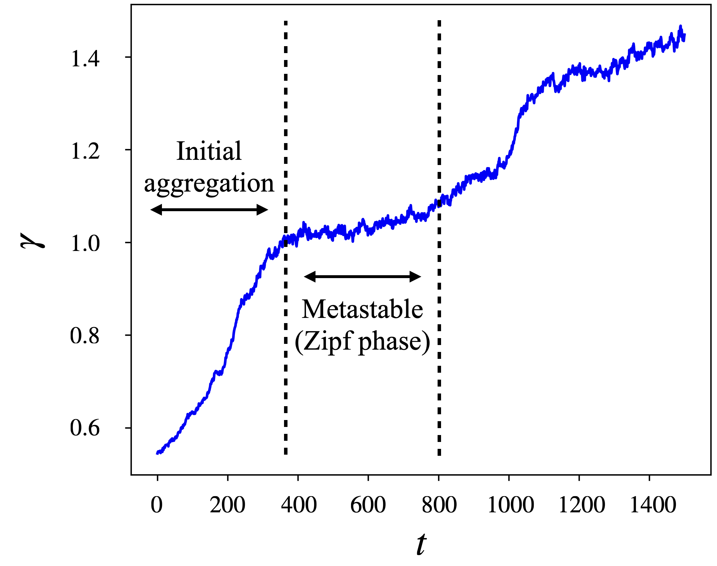
Furthermore, the rank-size distribution is in a steady state past $t=400$ (Fig. 4). To investigate its long-term behavior, we plotted the evolution of the mean rank-size exponent over a longer period (Fig. 5). Note that $r^{2}$ values score more than $0.96$ at any measured moment. We find that in an initial stage (from $t=0$ to $t\approx 350$), the exponent $\gamma$ generally increases monotonically as a result of aggregation. However, the rate of increase exhibits a significant slowdown, followed by a relatively long period (from $t\approx 350$ to $800$) during which the exponent remains, which we call a “Zipf phase.”

As shown in Fig. 5, however, the exponent starts growing again after the Zipf phase, especially with a characteristic sudden increase at around $t=1000$. During and after the Zipf phase, even established clusters constantly fluctuate owing to the random force in Eq. (5), and smaller clusters potentially merge into nearby larger ones, which causes a sudden increment in the value of the exponent. Therefore, we suggest that Zipf’s law does not necessarily represent an equilibrium (as usually discussed in the literature Gabaix and Ioannides (2004); Hsu (2008); Arshad et al. (2018)) but rather a metastable state with large fluctuations that might free the society from being trapped. Although the exact time and value of the exponent at which noticeable slowdowns in the rate of increase occur vary from time to time (due to different initial conditions and randomness in the motion of agents), such declines and the consequent metastability of the aforementioned phenomenon appears typical in most cases. Our discussion on metastability may provide a clue as to why many urban systems have their rank-size exponents close to 1 but still demonstrate an overall increasing tendency, as discussed in Sec. I.

Figure 6: Anti-correlation between changes in the unemployment rate and corresponding growth rates in the production output obtained from the same data as in Fig. 2 (from $t=0$ through $t=600$). The plotted data (circles) are regressed linearly (solid line).

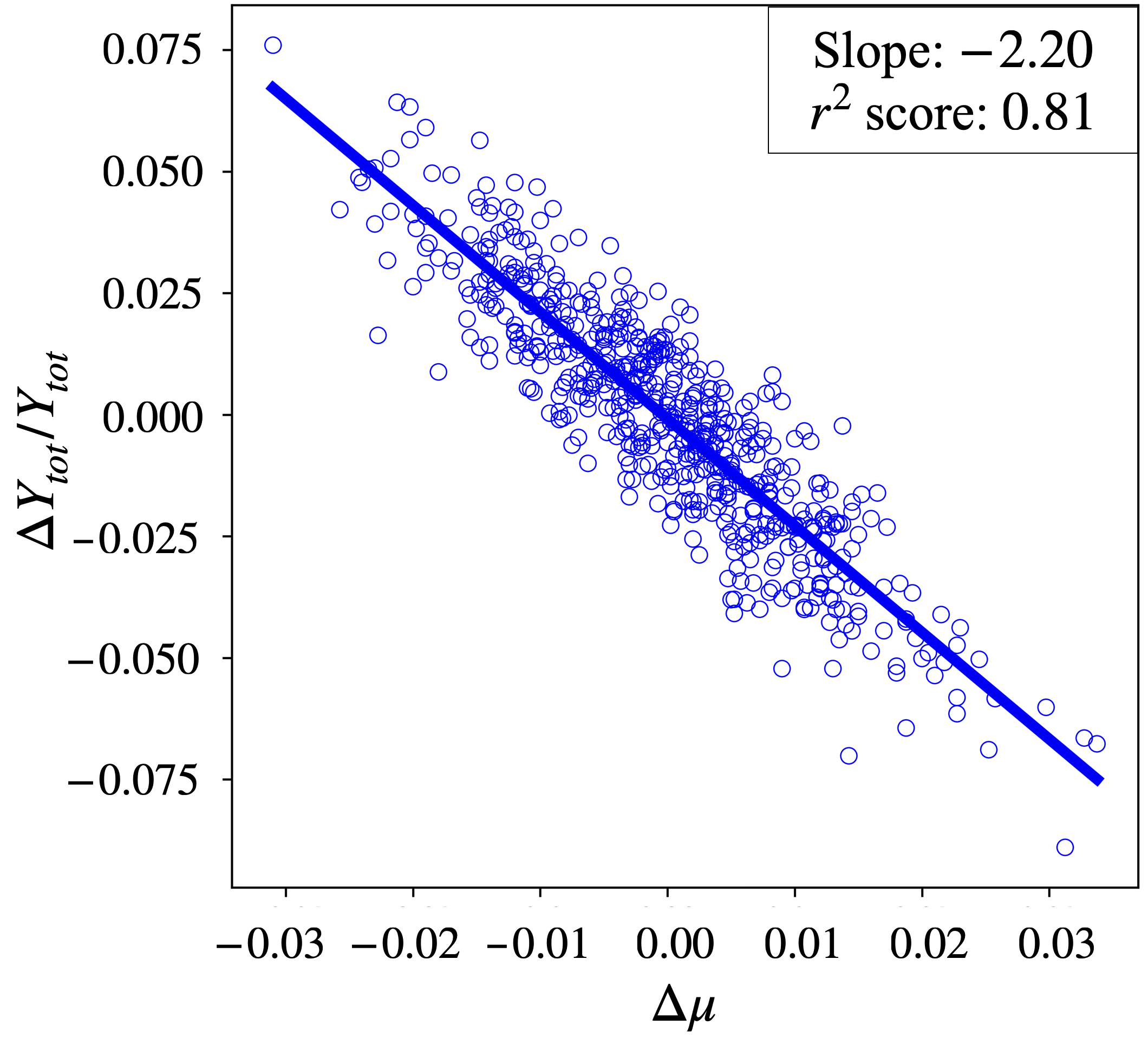
To understand how labor mobility relates to economic circumstances in our model, we investigated the relationship between changes in the unemployment rate and growth rates in the total output (Fig. 6). In the figure, data are plotted in the $\Delta\mu-\Delta Y_{tot}/Y_{tot}$ plane, where each dot represents the relationship between these two variables at each time step. The data demonstrate a clear anti-correlation between those two variables, and the regressed line has a slope of $-2.20$ with an $r^{2}$ score of $0.81$. For example, the reproduced value of the slope is highly reminiscent of Okun’s coefficient in the U.S. economy, which is estimated to be around $2$, as mentioned in Sec. I. Traditional theoretical explanations of the law tend to overestimate the coefficient Ball et al. (2013). The ability of our model to reproduce a reasonable coefficient may be indicative of its proper underlying mechanisms.

III.3 Econotaxis

In Sec. III.1, we stated that our model reproduces aggregations of agents. It is significantly characterized by the orientational movements of unemployed agents in response to their potential socio-economic advantages. This process can be understood as a positive taxis that emerges in social contexts. Taxis is often referred to, in biology literature, as a behavioral response in which an organism directs its movement in response to an external stimulus Stevens and Othmer (1997). Mathematically, it is described by a biased random walk Grünbaum (1998). In our model, the characteristic movement of unemployed agents is particularly initiated by a local economic activity in which employed agents are engaged. Therefore, we call this positive feedback process involved in our model “econotaxis.” Note that econotaxis is in line with the idea of self-reinforcement in urbanization, which some traditional theories have implied but not necessarily modeled explicitly Boddy (1999); Krugman (1991, 1992); Ottaviano and Thisse (2004).

Furthermore, we can derive the following Fokker–Planck equations from our microscopic model Risken (1996):

$$n_{t} =D_{n}\,\nabla^{2}n-\nabla\cdot\left(nf\right)-k^{+}n+k^{-}l,$$ (10)

$$l_{t} =D_{l}\,\nabla^{2}l+k^{+}n-k^{-}l,$$ (11)

where the densities of unemployed and employed agents are denoted by $n(r,t)$ and $l(r,t)$, respectively. The aforementioned macroscopic system indicates that our model reproduces the agglomeration of agents in a manner that is fundamentally similar to how the classical Keller–Segel system Keller and Segel (1970); Horstmann (2003) initiates aggregation phenomena called chemotaxis, a popular type of taxis by which certain chemicals affect cell migration. The Keller–Segel system is composed of two variables: $u,v$, the density of cells and the concentration of chemicals, given by

$$u_{t} =d_{u}\nabla^{2}u-\nabla\cdot\left(u\,\nabla\chi(v)\right),$$ (12)

$$v_{t} =d_{v}\nabla^{2}v+au-bv,$$ (13)

where $\chi(v)$ is called a sensitivity function that determines how migrating cells react to the chemoattractants.

The connection of Eqs. (12) and (13) to Eqs. (10) and (11) in terms of aggregation is apparent, which allows us to make at least two further arguments. First, the previously described investigation offers an interesting perspective on the nature of the labor force in general. Comparing econotaxis with chemotaxis, employed and unemployed agents can be identified as chemoattractants and cells, respectively. This suggests that although workers and jobless agents may sound like complete opposites, they play complementary roles during the aggregation process: employed agents function as “attractants,” helping the unemployed navigate the world to enable them to live off better employment opportunities. In other words, unemployed agents receive from employed agents a “signal” of benefit for their survival (i.e., employment opportunities) and respond to it while they constantly switch roles. Their well-coordinated and intertwined relationship amplifies the initial small heterogeneity and allows certain places to come out as highly populated. In this manner, our model suggests urban areas may emerge out of nowhere in human society.

Second, a vast amount of analytic investigation has revealed that many (often biological) chemotactic behaviors modeled by systems such as Eqs. (12) and (13) can be understood mathematically as blow-up phenomena Horstmann (2003); Hillen and Painter (2009); Arumugam and Tyagi (2021). This indicates that econotaxis is also related to blow-up phenomena in the system of Eqs. (10) and (11). From a sociological perspective, it may provide a potential answer to a long-standing question in urban science: Is there a saturation point in urbanization (i.e., an “urban maturity”)? Tisdale (1941); Berry (2008). The social science literature states that whether the process reaches equilibrium is still unknown, even though some are in favor of the idea of saturation Tisdale (1941); Berry (2008); Fujita and Thisse . Our numerical results with the new concept of econotaxis suggest otherwise: urbanization, thus, can be a relentless process.

IV Discussion & conclusions

In Secs. II and III.1, we developed a simple model of labor migration and demonstrated that agglomeration is an inherent characteristic. That might cast doubt on the major economic theory that increasing returns to scale (i.e., $\beta>1$ in Eq. (7)) is a prerequisite for urban agglomeration Fujita and Thisse (1996); Duranton and Puga (2004). Instead, our model suggests that a straightforward concave production function can cause agglomeration. In addition, the results in Sec. III.2 imply that the two well-known regularities may not arise from specific details of social or economic interactions but rather from the mechanism underlying agglomeration. The relationship between aggregation and transition probabilities is yet to be fully uncovered, which is worthy of further investigation. Based on our initial observation in Fig. 3 and Sec. III.1, aggregation behavior appears to be most facilitated when $k^{+}\approx k^{-}$. Although this speculation is appropriate in the short run (until $t\approx 200$), it is, in fact, not the case in the long run, especially after agents form clusters for the first time, and this is currently being investigated.

In summary, we have presented a simple microscopic model of urbanization to reveal the underlying fundamental mechanism. Despite its simplicity, the model initiated the aggregation of agents and reproduced some statistical regularities in human societies and economies. We then proposed a novel concept called econotaxis to characterize the self-assembly of the labor force. We also revealed the complementary roles played by employed and unemployed agents during the process of aggregation. Our model provides a unified theoretical approach to the study of urbanization and insight into the possibility that macroscopic agglomeration phenomena and Zipf’s and Okun’s laws lead to the same underlying mechanism, which has rarely been discussed before.

In future, the present model may even be able to reproduce some of the unique features of urban agglomeration, such as the U.S. manufacturing belt or Europe’s hot banana Krugman (2011), just by introducing geographical heterogeneity or spatial constraints. Other possible ways to extend our model include incorporating “congestion effects” Berry (2008); Boddy (1999) (i.e., effects of increase in dispersion as the place gets more crowded), considering an in- and outflux of population or intrinsic population growth and explicitly considering multiple industries. A possible limitation, however, is that the continuous models $(\ref{eq: nt})$ and $(\ref{eq: lt})$ are currently not likely to reproduce Zipf’s and Okun’s laws, as blow-up phenomena are expected to occur. Nonetheless, our model essentially replicates agglomeration phenomena as well as some empirically observed regularities while keeping itself mathematically tractable. We believe that it captures the underlying mechanism of urbanization at the most fundamental level. We hope that it will be a window into more complex structures and organizations that coordinate our society, encouraging theoretical and empirical research on social dynamics.

V Acknowledgements

I would like to thank Prof. Kota Ikeda (Meiji University, Japan) for insightful discussions and his comments on the manuscript. I am also grateful to Dr. Ryu Fujiwara (Meiji University) and Prof. Hiraku Nishimori (Meiji Institute for Advanced Study of Mathematical Sciences, Japan) for their helpful comments. I would like to thank Editage (www.editage.jp) for English language editing.

References

- Tisdale (1941) H. Tisdale, Soc. F. 20, 311 (1941).
- Berry (2008) B. J. Berry, in Urban ecology (Springer, 2008) pp. 25–48.
- Boddy (1999) M. Boddy, Urban studies 36, 811 (1999).
- Ottaviano and Thisse (2004) G. Ottaviano and J.-F. Thisse, in Handbook of regional and urban economics, Vol. 4 (Elsevier, 2004) pp. 2563–2608.
- Fujita and Thisse (2002) M. Fujita and J.-F. Thisse, Available at SSRN 315966 (2002).
- Fujita and Thisse (1996) M. Fujita and J.-F. Thisse, Journal of the Japanese and international economies 10, 339 (1996).
- Brakman and Garretsen (2003) S. Brakman and H. Garretsen, Regional Studies 37, 637 (2003).
- Grotewold (1959) A. Grotewold, Economic Geography 35, 346 (1959).
- Mäki (2004) U. Mäki, Environment and Planning A 36, 1719 (2004).
- Isard (1949) W. Isard, The Quarterly Journal of Economics 63, 476 (1949).
- Capello (2014) R. Capello, in Handbook of regional science (Springer, 2014) pp. 507–526.
- King (2020) L. J. King, (2020).
- Mulligan (1984) G. F. Mulligan, International Regional Science Review 9, 1 (1984).
- Martin (1999) R. Martin, Transactions of the Institute of British Geographers 24, 387 (1999).
- Glaeser (2010) E. L. Glaeser, Agglomeration economics (University of Chicago Press, 2010).
- Puga (2010) D. Puga, Journal of regional science 50, 203 (2010).
- Duranton and Puga (2004) G. Duranton and D. Puga, in Handbook of regional and urban economics, Vol. 4 (Elsevier, 2004) pp. 2063–2117.
- Krugman (1992) P. Krugman, A dynamic spatial model, Tech. Rep. (National Bureau of Economic Research, 1992).
- Scott (2006) A. J. Scott, in Economic Geography (Routledge, 2006) pp. 78–102.
- Castellano et al. (2009) C. Castellano, S. Fortunato, and V. Loreto, Reviews of modern physics 81, 591 (2009).
- Gonzalez et al. (2008) M. C. Gonzalez, C. A. Hidalgo, and A.-L. Barabasi, nature 453, 779 (2008).
- Schläpfer et al. (2021) M. Schläpfer, L. Dong, K. O’Keeffe, P. Santi, M. Szell, H. Salat, S. Anklesaria, M. Vazifeh, C. Ratti, and G. B. West, Nature 593, 522 (2021).
- Shida et al. (2020) Y. Shida, H. Takayasu, S. Havlin, and M. Takayasu, Scientific reports 10, 1 (2020).
- Schweitzer (2002) F. Schweitzer, in Modeling complexity in economic and social systems (World Scientific, 2002) pp. 137–159.
- Schweitzer (2003) F. Schweitzer, Brownian agents and active particles: collective dynamics in the natural and social sciences (Springer Science & Business Media, 2003).
- Romanczuk et al. (2012) P. Romanczuk, M. Bär, W. Ebeling, B. Lindner, and L. Schimansky-Geier, The European Physical Journal Special Topics 202, 1 (2012).
- Schimansky-Geier et al. (1995) L. Schimansky-Geier, M. Mieth, H. Rosé, and H. Malchow, Physics Letters A 207, 140 (1995).
- Helbing (2001) D. Helbing, Reviews of modern physics 73, 1067 (2001).
- Hinloopen and van Marrewijk (2006) J. Hinloopen and C. van Marrewijk, Comparative advantage, the rank-size rule, and Zipf’s law, Tech. Rep. (Tinbergen Institute Discussion Paper, 2006).
- Rose (2005) A. K. Rose, “Cities and countries,” (2005).
- Gabaix and Ioannides (2004) X. Gabaix and Y. M. Ioannides, in Handbook of regional and urban economics, Vol. 4 (Elsevier, 2004) pp. 2341–2378.
- Veneri (2016) P. Veneri, Computers, Environment and Urban Systems 59, 86 (2016).
- Reed (2002) W. J. Reed, Journal of Regional Science 42, 1 (2002).
- Gabaix (1999) X. Gabaix, The Quarterly journal of economics 114, 739 (1999).
- Simon (1955) H. A. Simon, Biometrika 42, 425 (1955).
- Cristelli et al. (2012) M. Cristelli, M. Batty, and L. Pietronero, Scientific reports 2, 1 (2012).
- Wang and Chen (2021) J. Wang and Y. Chen, Sustainability 13, 3287 (2021).
- Guérin-Pace (1995) F. Guérin-Pace, Urban studies 32, 551 (1995).
- Okun (1963) A. M. Okun, Potential GNP: its measurement and significance (Cowles Foundation for Research in Economics at Yale University, 1963).
- Lee (2000) J. Lee, Journal of macroeconomics 22, 331 (2000).
- Knotek II (2007) E. S. Knotek II, Economic Review-Federal Reserve Bank of Kansas City 92, 73 (2007).
- Cuaresma (2003) J. C. Cuaresma, Oxford Bulletin of Economics and Statistics 65, 439 (2003).
- Ball et al. (2013) L. M. Ball, D. Leigh, and P. Loungani, Okun’s law: fit at fifty?, Tech. Rep. (National Bureau of Economic Research, 2013).
- (44) M. Fujita and J.-F. Thisse, Economics of Agglomeration: Cities, Industrial Location, and Globalization.
- Nutter Jr (2010) F. W. Nutter Jr, Encyclopedia of research design 3, 1612 (2010).
- Hsu (2008) W.-T. Hsu, Central place theory and Zipf’s law, Ph.D. thesis, Citeseer (2008).
- Arshad et al. (2018) S. Arshad, S. Hu, and B. N. Ashraf, Physica A: Statistical mechanics and its applications 492, 75 (2018).
- Stevens and Othmer (1997) A. Stevens and H. G. Othmer, SIAM Journal on Applied Mathematics 57, 1044 (1997).
- Grünbaum (1998) D. Grünbaum, Evolutionary Ecology 12, 503 (1998).
- Krugman (1991) P. Krugman, Journal of political economy 99, 483 (1991).
- Risken (1996) H. Risken, in The Fokker-Planck Equation (Springer, 1996) pp. 63–95.
- Keller and Segel (1970) E. F. Keller and L. A. Segel, Journal of theoretical biology 26, 399 (1970).
- Horstmann (2003) D. Horstmann, (2003).
- Hillen and Painter (2009) T. Hillen and K. J. Painter, Journal of mathematical biology 58, 183 (2009).
- Arumugam and Tyagi (2021) G. Arumugam and J. Tyagi, Acta Applicandae Mathematicae 171, 1 (2021).
- Krugman (2011) P. Krugman, Regional studies 45, 1 (2011).