Four Lectures on the Random Field Ising Model,
Parisi-Sourlas Supersymmetry,
and Dimensional Reduction

Abstract

Numerical evidence suggests that the Random Field Ising Model loses Parisi-Sourlas SUSY and the dimensional reduction property somewhere between 4 and 5 dimensions, while a related model of branched polymers retains these features in any $d$. These notes give a leisurely introduction to a recent theory, developed jointly with A. Kaviraj and E. Trevisani, which aims to explain these facts. Based on the lectures given in Cortona and at the IHES in 2022.

1 History, Basics, Experiments and Simulations

1.1 History

The Random Field Ising Model (RFIM) is the Ising model coupled to a random $x$-dependent magnetic field. It was introduced in 1975 by Imry and Ma ImryMa , who predicted a phase transition in $d>2$ but not in $d\leqslant 2$, via the Imry-Ma argument discussed below. Imry and Ma also found the upper critical dimension $d_{{\rm uc}}=6$.

In 1976, Aharony, Imry and Ma Aharony:1976jx found that, to all orders in perturbation theory, the RFIM critical exponents in $d=6-\varepsilon$ dimensions are the same as the critical exponents of the usual Ising model in $d-2$ dimension. This became known as the dimensional reduction of critical exponents.

In 1979, Parisi and Sourlas Parisi:1979ka found that RFIM has an equivalent supersymmetric formulation. They showed that dimensional reduction is a natural consequence of supersymmetry (SUSY).

These developments immediately led to a puzzle when extrapolating to the physical dimension $d=3$. Dimensional reduction cannot be true in this dimension, since the $d=1$ Ising model does not even have a phase transition. Perturbation theory is apparently breaking down somewhere between $d=6$ and 3. Why?

Over the subsequent decades, there were many attacks on this problem. In particular, Brézin and De Dominicis Brezin-1998 in 1998, and Feldman Feldman in 2000 argued that dimensional reduction breaks down for any $d<6$, because of subtle RG effects. Tarjus and Tissier Tarjus2004 in 2004 found, in a nonperturbative RG calculation, that dimensional reduction holds for $d>d_{c}\approx 5.1$ but breaks down at $d<d_{c}$. While we do not fully agree with these authors, we will make contact with some of their ideas below.

The RFIM phase transition in $d=3$ was studied both experimentally BelangerYoung and via numerical simulations (the only way available in $d>3$). For $d=4$ and $d=5$, the critical exponents were determined by Fytas, Martín-Mayor, Picco and Sourlas in 2016. These studies led to an interesting conclusion. In $d=4$, dimensional reduction is clearly ruled out Picco1 . On the other hand, the $d=5$ model shows not only the dimensional reduction of critical exponents Picco2 , but was also found in their later work Picco3 (joint with Parisi) to respect SUSY relations between correlation functions, providing a direct test of SUSY.

These lectures will explain a theory developed in collaboration with Apratim Kaviraj and Emilio Trevisani paper1 ; paper2 ; paper-summary ; paper3 , which started in 2018 and was sparked by a conference on disordered systems in Rome. Our main conclusions are these:

• Dimensional reduction is lost because SUSY is lost.

• SUSY is lost because some SUSY-breaking perturbations, present at the microscopic level, become relevant at $d<d_{c}$ (while they are irrelevant at $d>d_{c}$).

• From two-loop perturbation theory, we estimate $d_{c}\approx 4.5$. This is in good agreement with the above-mentioned numerical simulations, that dimensional reduction is lost between 4 and 5 dimensions.

1.2 Basic facts

Recall that the usual Ising model in $d\geqslant 2$ dimensions has a phase transition at a critical temperature $T_{c}>0$. For $T>T_{c}$ the model is in the disordered phase of vanishing magnetization. For $T<T_{c}$ the model is in the ordered phase, and the magnetization is nonzero: $m(T)>0$. The magnetization $m$ can be defined e.g. as an infinite volume limit of the average spin value at a point in the middle of the lattice with the $+$ boundary conditions:

$$m=\lim_{L\rightarrow\infty}\langle s_{0}\rangle_{+}.$$ (1)

The phase transition is continuous: $m(T)\rightarrow 0$ as $T\rightarrow T_{c}$.

The usual Ising model is a model for pure uniaxial ferromagnets. Real materials however always contain impurities, also known as disorder effects. Superclean electronics-grade silicon has 1 impurity per $10^{9}$ atoms. This means that the average distance between impurities is $O(10^{3})$, which is not such a huge number.

Consider then uniaxial ferromagnets with impurities. In these lectures we will be interested in magnetic impurities. These can be modeled by adding a local $x$-dependent magnetic field. The Hamiltonian of the model becomes

$$\mathcal{H}[s,h]=-J\sum_{\langle xy\rangle}s_{x}s_{y}-\sum_{x}h_{x}s_{x},$$ (2)

where $h_{x}$ is the magnetic field created by impurities at site $x$. We will be interested in the case when $h$ can be considered frozen (not in thermal equilibrium with $s$). Such a form of disorder is called quenched. For a given $h$, we can then define the partition function

$$Z[h]={\rm Tr}_{s}e^{-\beta\mathcal{H}[s,h]},$$ (3)

and correlation functions, e.g.

$$\langle s_{x}s_{y}\rangle_{h}=Z[h]^{-1}{\rm Tr}_{s}\,s_{x}s_{y}\,e^{-\beta\mathcal{H}[s,h]}.$$ (4)

The next step is to replace a fixed disorder instance $h$ by a random one. The rationale behind this is that a large system can be divided into many chunks which are still large. Each chunk will have its own disorder instance, and these instances can be assumed statistically independent, drawn from some distribution $\mathcal{P}[h]$ (assuming, as we will, that faraway impurities do not influence each other). Thus, any quantity involving an average over the volume can be computed as an average over $\mathcal{P}[h]$. Such quantities are called self-averaging. Examples include the free energy and volume-averaged correlation functions, such as

$$\frac{1}{V}\sum_{x}\langle s_{x}s_{x+r}\rangle_{h}.$$ (5)

We will assume that $\mathcal{P}[h]$ respects lattice symmetries (translations and rotations). We will also impose $\mathbb{Z}_{2}$ invariance: $\mathcal{P}[h]=\mathcal{P}[-h]$. This means that magnetic impurities have no preferred orientation. In particular we have (denoting averages w.r.t. $\mathcal{P}[h]$ by an overbar)

$$\overline{h_{x}}=0.$$ (6)

As we said, the two-point correlation function of the disorder, $\overline{h_{x}h_{y}}=f(x-y)$ is assumed short-ranged.

Definition.

The Random Field Ising Model is the Ising model coupled to a random magnetic field $h$, drawn from a distribution $\mathcal{P}[h]$ which is $\mathbb{Z}_{2}$-invariant, translationally and rotationally invariant, and has short-range correlations. Correlation functions of the model are computed by first averaging over $s$, then over $h$, e.g.

$$\overline{\langle s_{x}s_{y}\rangle_{h}}=\overline{Z[h]^{-1}{\rm Tr}_{s}s_{x}s_{y}e^{-\beta\mathcal{H}[s,h]}}.$$ (7)

We may assume for simplicity that

$$\mathcal{P}[h]=\prod_{x}P[h_{x}],$$ (8)

i.e. that $h_{x}$ are i.i.d. random variables. Then we have

$$\overline{h_{x}h_{y}}=0\quad(x\neq y),\qquad\overline{(h_{x})^{2}}=\kappa^{2},$$ (9)

where the parameter $\kappa$ measures disorder strength. We may simplify further and assume that the distribution $P[h_{x}]$ is Gaussian:

$$P[h_{x}]=\frac{1}{\sqrt{2\pi}\kappa}e^{-h_{x}^{2}/(2\kappa^{2})}.$$ (10)

The usual justification for all these simplifying assumptions is universality. Normally, it is believed that models corresponding to different $P[h_{x}]$ will flow to the same renormalization group fixed point describing the transition.

The phase diagram of the model in $d>2$ contains an ordered phase at small $T$ and small $\kappa$, and a disordered phase at large values of these parameters (see Fig. 1). The magnetization order parameter can be defined similarly to (1) for the pure Ising case, namely as an infinite-volume limit of a single-spin correlation function with the $+$ boundary conditions:

$$m=\lim_{L\rightarrow\infty}\overline{\langle s_{0}\rangle_{+}}\,.$$ (11)

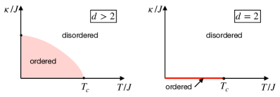
Figure 1: The RFIM phase diagram for $d>2$ (left) and $d=2$ (right).

On the other hand, in $d=2$ the model is disordered for an arbitrarily small $\kappa$ (see Fig. 1). The difference between $d=2$ and $d=3$ is understood via the Imry-Ma argument ImryMa , a kind of Peierls’ argument in presence of disorder. As in Peierls’ argument, one studies the possibility to disorder the all $+$ state by inverting droplets. The energy cost of inverting a droplet $U$ of linear size $R$ is proportional to the surface area $\delta E_{1}\sim J|\partial U|\sim JR^{d-1}$. In Peierls’ argument, this cost is offset by entropy effects at nonzero temperature, in $d=1$ (but not in $d\geqslant 2$). In the Imry-Ma argument one works at zero temperature, and one tries to offset $\delta E_{1}$ by the magnetic field contribution $\delta E_{2}=2\sum_{x\in U}h_{x}$. We have $\overline{(\delta E_{2})^{2}}\sim\kappa^{2}|U|$, i.e. $\delta E_{2}$ has typical size $\delta E^{{\rm typ}}_{2}=\pm\kappa R^{d/2}$.

We would like to find a droplet surrounding $x=0$ such that $\delta E_{1}+\delta E_{2}<0$. We are assuming that $\kappa\ll J$ (weak disorder), so this is unlikely for small droplets. For large droplets, the ratio $\delta E^{{\rm typ}}_{2}/\delta E_{1}$ decreases with $R$ for $d>2$. We conclude that the ordered state survives for $d>2$ for weak disorder. For $d=2$, the ratio $\delta E^{{\rm typ}}_{2}/\delta E_{1}$ stays constant with $R$. For any $R$, there is a small finite chance to find a droplet of this size surrounding $x=0$ which can be flipped lowering the energy. In a sufficiently large volume, there will be many values of $R$ to consider, and the probability to find a good droplet tends to 1. This shows that the model is disordered for $d=2$.

From now on, we will focus on $d>2$. Our main interest will be the phase transition which happens along the line separating the ordered and the disordered phases. It is believed that this transition is continuous. Moreover, it is believed that the whole line, excluding the point $\kappa=0$, $T=T_{c}$, belongs to the same universality class. The schematic RG flow diagram corresponding to this picture is shown in Fig. 2. We have two fixed points. The pure Ising fixed point (I) is at $\kappa=0$, $T=T_{c}$. It is unstable with respect to disorder perturbations. All points on the transition line flow to the Random Field fixed point (RF) located at $T=0$, $\kappa=\kappa_{c}$.

Figure 2: RG flow along the phase separation line from the pure Ising fixed point I to the Random Field fixed point RF, located at zero temperature.

Literature and further comments

For a textbook exposition, see Cardy Cardy-book .

Another way to understand that the $d=2$ model is disordered is via RG. One can argue Bray1985 that the ratio $w=\kappa/J$ satisfies in $d=2$ an RG equation $dw/d\ell=Aw^{3}$, $A>0$. Thus any weak disorder grows and becomes strong at long distances.

Rigorous mathematical work confirmed the RFIM phase diagram following from the Imry-Ma argument. Imbrie imbrieLCD2 proved in 1985 that the RFIM in $d=3$ is ordered at weak $\kappa$ and $T=0$. Bricmont and Kupiainen BK showed in 1988 that the order persists in $d=3$ at weak $\kappa$ and small nonzero $T$. Recently there were some new developments. A new and simple proof of the Imbrie and Bricmont-Kupiainen results was given in 2021 by Ding and Zhuang Ding1 . Further work Ding showed that order persists at all $T<T_{c}$ and sufficiently small $\kappa$.

Disorder in $d=2$ at arbitrarily small $\kappa$ was also shown to hold rigorously, by Aizenman and Wehr Aizenman1990 in 1990. See also Ding2 for recent rigorous developments in $d=2$.

1.3 Experiments

Experimental studies of the RFIM in $d=3$ and $d=2$ were nicely reviewed in 1991 by Belanger and Young BelangerYoung (see also Belanger ). 2d experiments confirm the absence of a phase transition. Here we will focus on the 3d case, where three experimental platforms exist.

Site-diluted uniaxial antiferromagnets in a uniform magnetic field. The microscopic Hamiltonian of this model is:

$$\mathcal{H}=J\sum_{\langle xy\rangle}\varepsilon_{x}\varepsilon_{y}s_{x}s_{y}+H\sum_{x}\varepsilon_{x}s_{x},$$ (12)

where $s_{x}$ are the Ising spins, while $\varepsilon_{x}\in\{0,1\}$ are disorder variables showing that some sites are vacant. They are chosen at random, to satisfy a chosen concentration of vacancies. We see that this is a disordered model, but the form of a disorder is different from RFIM. For the zero uniform field, $H=0$, this model on the cubic lattice is in the universality class of the bond-disordered Ising model (footnote 1). For nonzero $H$, the phase transition should be in the RFIM universality class, as was shown by Fishman and Aharony Fishman and by Cardy Cardy-site-diluted . The idea is that nonzero $H$ creates a uniform magnetization, on top of the antiferromagnetic order parameter experiencing the critical fluctuations. The uniform magnetization couples linearly to the order parameter, with a strength which is random since it depends on the local dilution strength. The uniform magnetization times the random coupling strength plays the role of a random magnetic field in RFIM. In this setup, the effective random magnetic field strength can be tuned continuously by varying $H$.

Experimentally, site-diluted uniaxial antiferromagnets can be realized by replacing magnetic ions of a pure antiferromagnet by nonmagnetic ones. E.g. replacing some Fe ions in ${\rm Fe}\text{F}_{2}$ by ${\rm Zn}$ one obtains a site-diluted antiferromagnet ${\rm Fe}_{x}{\rm Zn}_{1-x}\text{F}_{2}$ where $x$ is the remaining concentration of ${\rm Fe}$ ions. Replacement happens at random when the crystal is grown. Experiments in such 3d materials showed a continuous phase transition Belanger .

Structural phase transitions. In this context, one takes a pure crystal which undergoes a transition of the Ising universality class. One then adds impurities coupling linearly to the order parameter. One example is the compound ${\rm Dy}\,\text{V}\,\text{O}_{4}$ which has tetragonal crystal lattice at high temperature, deforming to orthorhombic at lower temperature. Deformation can happen in two orthogonal directions, and the order parameter has $\mathbb{Z}_{2}$ symmetry as needed (Fig. 3). This phase transition is known to be driven by the linear coupling of electronic states of Dy and of the lattice modes (the Jahn-Teller effect Jahn-Teller ). Replacing some of the V atoms by As one gets a disordered crystal ${\rm Dy}\text{As}_{x}\,\text{V}_{1-x}\,\text{O}_{4}$, which realizes the RFIM. Measurements with this crystal found a continuous phase transition GrahamJT .

Figure 3: Structural phase transition in pure ${\rm Dy}\,\text{V}\,\text{O}_{4}$. Left: The primitive cell of the tetragonal lattice is a square prism. Right: (View from above) At low temperatures the square section of the prism gets deformed to a rectangle. This can happen along the two axes, with the two ground states related by $\mathbb{Z}_{2}$.

Binary fluids in a gel. Binary fluids are mixtures of two different fluids, A and B, which are miscible in a range of temperatures $T$ and concentration $x$. The typical phase diagram is in Fig. 4. The point C in that diagram is a critical point, in the Ising universality class. The fluctuating order parameter of this system is the local deviation of the concentration from the critical value.

Figure 4: A typical phase diagram of a binary fluid.

A gel is a rigid random network of polymer molecules. The randomness is built when fabricating a gel. Imagine saturating a gel with a binary fluid, and assume that the interaction between the gel and the molecules of the two fluid components is not identical. Then, the presence of the gel will act as a random field coupled linearly to the order parameter of the binary fluid, as discussed by de Gennes in 1984 DeGennes1984 . If long-range correlations in the gel structure can be neglected, the phase transition in such a system should be of the RFIM universality class. Experimentally this setup was studied in Sinha1991 .

1.4 Numerical simulations

Naively one might think that simulating RFIM is a hopeless task. On top of the usual challenges of a Monte Carlo simulation at a finite temperature, arising from the need to thermalize the system in a large volume and generate a large number of statistically independent configurations, one seems to face the task to repeat all of this for many instances of the magnetic field $h$. However there is a trick which saves the day for the RFIM. Namely, the fixed point controlling the phase transition is at zero temperature (Fig. 2). Thus, we may simulate the model directly at $T=0$. At $T=0$, there is no need to thermalize. Instead, we only need to find the ground state.

The simulation proceeds as follows. We fix the disorder distribution shape, e.g. the Gaussian (10). We choose the disorder strength $\kappa$. For the chosen $\kappa$, we repeat many times the following two steps: (1) generate an instance of a random field $h_{x}$ for every point $x$ on the (large but finite) lattice; (2) find the ground state, i.e. a configuration of spins minimizing the RFIM Hamiltonian. We then vary $\kappa$ and tune it, until we find the critical value $\kappa_{c}$ corresponding to the phase transition.

Note that the ground state on a finite lattice is unique for all choices of $h$ but a set of measure zero. Indeed, suppose there are two ground states $s_{1}$ and $s_{2}$, $\mathcal{H}[s_{1},h]=\mathcal{H}[s_{2},h]$. For any fixed $s_{1}\neq s_{2}$, the set of $h$’s solving this equation is a hyperplane, hence of measure zero.

The problem of finding the ground state for a given $h$ is equivalent to a classic problem of graph theory: finding a minimal cut in a graph. Let us add two vertices $A$ and $B$ to the lattice, assigning them spins $s_{A}=+1$ and $s_{B}=-1$. For vertices $x$ with $h_{x}>0$ we introduce a coupling $J_{xA}=h_{x}$ and for vertices $x$ with $h_{x}<0$ we introduce a coupling $J_{xB}=-h_{x}$. The RFIM Hamiltonian can now be rewritten equivalently as

$$\mathcal{H}[s,h]=-\sum_{\langle xy\rangle}J_{xy}s_{x}s_{y},$$ (13)

where the sum goes over the old bonds $J_{xy}=J$ and the new bonds $J_{xA}$ and $J_{xB}$. Crucially, all $J_{xy}>0.$

To minimize the energy written in this form, we need to find a boundary separating the $+$ spins from the $-$ spins such that the sum of all bonds $J_{xy}$ traversing the boundary is minimal. Note that the boundary is not empty since we assigned $s_{A}=+1$ and $s_{B}=-1$. Such a minimal separating boundary is called the minimal cut between the source $A$ and the sink $B$ (Fig. 5).

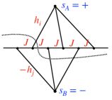
Figure 5: Finding the RFIM ground state is reduced to finding the minimal cut (dotted line). See the text.

The minimal cut in a graph with positive weights on each link can be found by efficient polynomial-time algorithms, such as e.g. the push-relabel algorithm. State-of-the-art numerical simulations of RFIM rely on such algorithms. For an excellent review of these algorithms and many problems in statistical physics they can be applied to (including RFIM), see Alava . To learn more about how the RFIM simulations are done, see the excellent review FytasReview .

In Table 1 we report the RFIM critical exponents obtained in numerical simulations and, for comparison, the exponents of the pure Ising model. Note that $\nu\left(\text{4d RFIM}\right)\neq\nu\left(\text{2d Ising}\right)$, hence no dimensional reduction in $d=4$. On the other hand, $\nu\left(\text{5d RFIM}\right)$ is remarkably close to $\nu\left(\text{3d Ising}\right)$. Also $\eta\left(\text{5d RFIM}\right)$ agrees, at $\sim 1.5\sigma$ level, with $\eta\left(\text{3d Ising}\right)$. These agreements suggest that the reduction may well hold in $d=5$. A further special property which appears to hold in $d=5$ is $\eta=\bar{\eta}$. We will see in Section 2.6 that this equality is a sign of the Parisi-Sourlas SUSY, which is closely related to dimensional reduction.

$d$	$\nu$	$\eta$	$\bar{\eta}$	Ref.
3	$1.38(10)$	0.5153(9)	$\approx 2\eta$	Fytas3
4	$0.872(7)$	0.1930(13)	$\approx 2\eta-0.0322(23)$	Picco1
5	$0.626(15)$	0.055(15)	$\approx\eta$	Picco2

$d$	$\nu$	$\eta$	Ref.
1	-	-	-
2	1	$1/4$	exact
3	0.629771(4)	0.036298(2)	Kos:2016ysd

Table 1: Critical exponents in the RFIM (above) and in the pure Ising model (below). Recall that $\nu$ controls the growth of the correlation length $\xi$ as $T\rightarrow T_{c}$. In the RFIM context at $T=0$, $\nu$ controls the growth of $\xi$ as $\kappa\rightarrow\kappa_{c}$: $\xi\sim|\kappa-\kappa_{c}|^{-\nu}$. The exponents $\eta$ and $\bar{\eta}$ will be discussed in Section 2.

2 Parisi-Sourlas theory, dimensional reduction

In this lecture we will study Parisi and Sourlas’s original argument Parisi:1979ka for the presence of SUSY at the RFIM critical point. We will discuss possible caveats. We will also see why the Parisi-Sourlas SUSY implies dimensional reduction.

2.1 Field theory and perturbation theory

At the critical point we may replace the lattice formulation of the model by a field theory. The appropriate field theory is a scalar field with quartic self-interactions and coupled to a random magnetic field:

$$S[\phi,h]=\int d^{d}x\left[\frac{1}{2}(\partial\phi)^{2}+V(\phi)-h\phi\right],\qquad V(\phi)=\frac{1}{2}m^{2}\phi^{2}+\frac{\lambda}{4!}\phi^{4},$$ (14)

$$\overline{h(x)h(x^{\prime})}=R\,\delta^{(d)}(x-x^{\prime}),$$ (15)

where the parameter $R$ plays the role of $\kappa^{2}$ in (9). Correlation functions are computed as

$$\overline{\langle A(\phi)\rangle_{h}}=\int\mathcal{D}h\,\mathcal{P}(h)\langle A(\phi)\rangle_{h},$$ (16)

$$\langle A(\phi)\rangle_{h}=\frac{\int\mathcal{D}\phi A(\phi)e^{-S[\phi,h]}}{Z[h]}$$ (17)

where $A(\phi)$ is any function of fields, and $\mathcal{P}(h)\propto e^{-\int d^{d}x\;h^{2}/(2R)}$.

We will consider perturbative expansion in this theory. Let us first discuss how to compute $\langle A(\phi)\rangle_{h}$ for a fixed $h$. We will then see what happens when we average over $h$.

For a fixed $h$, we have Feynman diagrams with the propagator $\langle\phi_{p}\phi_{-p}\rangle_{\lambda=0}=\frac{1}{p^{2}+m^{2}}$. In addition to the quartic interaction vertex $\lambda$, there is a vertex expressing the linear $h\phi$ coupling:

$$\raisebox{2.58334pt}{\raisebox{-0.5pt}{\includegraphics[height=27.0pt]{fig-hx.pdf}}}\text{(position space),}\qquad\raisebox{2.58334pt}{\raisebox{-0.5pt}{\includegraphics[height=26.0pt]{fig-hp.pdf}}}\text{(momentum space)}.$$ (18)

In quantum field theory, such linear vertices are called “tadpoles”. Since $h(x)$ is, in general, $x$-dependent, the momentum space vertex carries external momentum.

Due to tadpoles, $\phi$ acquires a nonzero $h$-dependent expectation value:

$$\langle\phi(x)\rangle_{h}=\raisebox{2.58334pt}{\raisebox{-0.5pt}{\includegraphics{fig-RFIM1-1.pdf}}}\,.$$ (19)

To make sure that the notation is clear, we will give just once a translation of these Feynman diagrams into an equation:

$$\langle\phi(x)\rangle_{h} = \int G(x-u)h(u)d^{d}u$$ (20)

$$+ \lambda^{2}\int G(x-y)G(y-z)^{3}G(z-u)h(u)d^{d}yd^{d}zd^{d}u$$

$$+ \lambda\int G(x-y)\prod_{i=1}^{3}G(y-u_{i})h(u_{i})d^{d}u_{i}d^{d}y+\ldots,$$

where $G(x)=\int\frac{d^{d}p}{(2\pi)^{d}}\frac{1}{p^{2}+m^{2}}e^{ipx}$ is the position-space propagator.

As another example, we will give the first few terms in the perturbative expansion of the two-point functions $\langle\phi\phi\rangle$:

$$\langle\phi(x)\phi(y)\rangle_{h}=\ \raisebox{-60.00009pt}{\includegraphics[scale={1.1}]{fig-phi-phi.pdf}}$$ (21)

In the first line we gave the terms present for $\lambda=0$ (Gaussian theory), in the second line the corrections involving $\lambda$ but not $h$, and in the third line corrections from both $\lambda$ and $h$.

Finally let us discuss what happens when we perform average over $h$. This average is denoted below by a dashed line. We do this average using the propagator (15), which becomes $\langle h_{p}h_{-p}\rangle=R$ in momentum space. In the Feynman diagram notation, this average means joining all crosses pairwise, in all possible combinations.

2.2 Connected and disconnected 2pt functions

The expression for $\langle\phi(x)\rangle_{h}$ in Eq. (19) has an odd number of crosses which cannot be paired, hence $\overline{\langle\phi(x)\rangle_{h}}=0$, as expected from $\mathbb{Z}_{2}$ symmetry.

On the other hand for $\overline{\langle\phi\phi\rangle_{h}}$ we obtain a nontrivial result. At $\lambda=0$ (Gaussian theory) we get, in momentum space

$$\overline{\langle\phi_{p}\phi_{-p}\rangle_{h}} =$$ (22)

$$= \frac{1}{p^{2}+m^{2}}+\frac{R}{(p^{2}+m^{2})^{2}}\qquad(\lambda=0).$$

This goes as $\sim R/p^{4}$ for $p\rightarrow 0$ at the critical point ($m^{2}=0$). Translating to position space, we get $\sim{\rm const}/r^{d-4}$ behavior for $r\rightarrow\infty$. This was for the Gaussian theory, while at the critical point of the interacting theory we will have a correction in the power, denoted $\bar{\eta}$:

$$G_{\text{disc}}(r):=\overline{\langle\phi(0)\phi(r)\rangle_{h}}=\frac{\text{const}}{r^{d-4+\bar{\eta}}}\quad(r\rightarrow\infty).$$ (23)

This is the disconnected 2pt function.

We can also consider a slightly different 2pt function:

$$\overline{\langle\phi(x)\rangle_{h}\langle\phi(y)\rangle_{h}}.$$ (24)

This quantity measures how expectation values of $\phi$ induced by the random field at two different points are correlated with each other. Unlike $\overline{\langle\phi(x)\rangle_{h}}$, this does not vanish. The result in the Gaussian theory is given by

$$\overline{\langle\phi_{p}\rangle_{h}\langle\phi_{-p}\rangle_{h}}=\raisebox{2.58334pt}{\raisebox{-0.5pt}{\includegraphics[scale={1.1}]{fig-phi-phi3.pdf}}}=\frac{R}{(p^{2}+m^{2})^{2}}\qquad(\lambda=0).$$ (25)

The connected 2pt function is defined by the difference:

$$G_{\text{conn}}(r):=\overline{\langle\phi(0)\phi(r)\rangle_{h}}-\overline{\langle\phi(0)\rangle_{h}\langle\phi(r)\rangle_{h}}\,.$$ (26)

This represented the susceptibility with respect to adding a localized non-random magnetic field:

$$G_{\text{conn}}(r)=\frac{\partial}{\partial H}\overline{\langle\phi(0)\rangle_{h+H\delta(x-r)}}.$$ (27)

Another rationale for the definition (26) is that the leading $p\rightarrow 0$ singularity cancels in the difference. Indeed in the Gaussian theory we will have $G_{\text{conn}}(p)=\frac{1}{p^{2}+m^{2}},$ which becomes $1/p^{2}$ at criticality, hence $\sim{\rm const}/r^{d-2}$ in the position space. So as usual, the connected 2pt function decays faster at infinity than the disconnected one.

In the interacting theory we expect that the critical behavior of $G_{\text{conn}}$ will be modified:

$$G_{\text{conn}}(r)=\frac{\text{const}}{r^{d-2+\eta}}\quad(r\rightarrow\infty).$$ (28)

In general, $\eta$ may be different from $\bar{\eta}$ from Eq. (23), and indeed we see from Table 1 that $\eta\neq\bar{\eta}$ in $d=3,4$. On the other hand, simulations in $d=5$ are consistent with $\eta=\bar{\eta}$. This, as we will see below, may be a sign of the Parisi-Sourlas SUSY.

Remark 2.1.

Let’s see the difference between the quenched disorder average (16) which treats the random magnetic field $h$ frozen, i.e. out of thermal equilibrium with $\phi$, and the usual average (called annealed disorder) which would consider $h$ as just another field in the path integral on par with $\phi$. In the latter case we would define correlation functions by

$$\langle A(\phi)\rangle_{{\rm ann}}=Z^{-1}\int\mathcal{D}h\mathcal{D}\phi A(\phi)e^{-S[\phi,h]-\int h^{2}/(2R)}.$$ (29)

Integrating out $h$, we are left with an action for the field $\phi$ alone, with a shifted mass: $m^{2}\rightarrow m^{2}-R$.

Not surprisingly, the values of correlation functions are completely different for the two procedures. Consider e.g. the disconnected 2pt function at $\lambda=0$. In the quenched case it is given by Eq. (22), while in the annealed case by

$$\langle\phi_{p}\phi_{-p}\rangle_{{\rm ann}}=\frac{1}{p^{2}+m^{2}-R}.$$ (30)

That’s clearly different from (22), although agrees to first order in $R$ at fixed $p$, but that’s not what matters. What matters is the behavior at $p\rightarrow 0$ when $m^{2}$ is fixed to the critical value. At criticality, the annealed 2pt function behaves as $1/p^{2}$ for $p\rightarrow 0$, while the quenched 2pt function shows a stronger $1/p^{4}$ singularity.

2.3 Selection of important diagrams

Let us study the structure of perturbative expansion in the interacting theory $(\lambda\neq 0)$. Consider first the pure Ising case $(h=0)$. It is interesting to consider the relative importance of loops vs tree level contributions. Compare these two diagrams contributing to the 4pt function:

$$\raisebox{2.58334pt}{\raisebox{-0.5pt}{\includegraphics[scale={1.1}]{fig-tree-loop.pdf}}}\,.$$ (31)

We can view the second diagram, involving an integral over the external loop momentum, as giving a correction $\delta\lambda=O(\lambda^{2})$ to the quartic coupling $\lambda$. At zero external momentum (as appropriate for studying the long-distance behavior of the model), $\delta\lambda/\lambda$ is given by:

$$\delta\lambda/\lambda=\lambda\int_{0}^{\Lambda}\frac{d^{d}k}{k^{4}},$$ (32)

where $\Lambda$ is the UV cutoff. For $d>4$, this integral converges at the lower limit. Thus $\delta\lambda/\lambda$ is finite. On the other hand, for $d<4$, the integral is IR-divergent. This is a simple way to identify the upper critical dimension of the model: $d_{\text{uc}}(\text{pure Ising})=4$.

For a nonzero external momentum $p$, the integral (32) will be IR-convergent and, for dimensional reasons, of order $\lambda p^{-\epsilon}$, where $\epsilon=4-d>0$. Further loops will introduce further factors of $\lambda p^{-\epsilon}$. Resumming these factors modifies the scaling behavior of correlators as $p\rightarrow 0$. Such resummation is usually performed by renormalization group methods, which convert fixed-order perturbative results into all-order expressions having good asymptotic scaling behavior.

Let us now apply similar logic to the RFIM. In addition to the above loop effects we will find new ones, more singular as $p\rightarrow 0$. Consider a few terms in the perturbative expansion of $\langle\phi(x)\rangle_{h}$:

$$\langle\phi(x)\rangle_{h}\ni\raisebox{2.58334pt}{\raisebox{-0.5pt}{\includegraphics{fig-phi-h-corr.pdf}}}.$$ (33)

The second diagram loop is a correction $\delta\lambda$ of the same form as for the pure Ising. But the last diagram, when averaging over $h$,  gives a new effect:

$$\includegraphics{fig-phi-h-corr1.pdf}\,.$$ (34)

We are imagining here that the crosses left free will connect to some other crosses as when computing $\overline{\langle\phi(x)\rangle_{h}\langle\phi(y)\rangle_{h}}$. We are focusing on just the shown subdiagram, which is of the same form the first diagram in (33), but with a coupling correction $\delta\lambda^{\prime}$,

$$\delta\lambda^{\prime}/\lambda=\lambda R\int_{0}^{\Lambda}\frac{d^{d}k}{k^{6}}.$$ (35)

This new correction is IR-divergent for $d<6$. Hence we conclude that the upper critical dimension of RFIM is raised to $d_{\text{uc}}(\text{RFIM})=6$.

When we compute any correlation function characterized by an external momentum $p$, the just described effect will cause, in the $n$-th order of perturbation theory, relative corrections of the order

$$(\lambda R)^{n}p^{-n\varepsilon}(1+O(p^{2}/R)),\qquad\varepsilon=6-d,$$ (36)

by dimensional analysis. Suppose we drop $O(p^{2}/R)$ correction in (36). This appears reasonable since we are interested in the $p\rightarrow 0$ limit (but see the caveats in Section 2.8 below). This corresponds to dropping “pure Ising” loop corrections like in the second diagram in (33) and keeping only the more singular loop corrections (34). This, in turn, means that before doing the average over $h$ we must keep, in each order in $\lambda$, the diagrams with the maximal number of crosses. These are the tree-level diagrams:

$$\phi_{h}(x):=\raisebox{2.58334pt}{\raisebox{-0.5pt}{\includegraphics[scale={1.1}]{fig-phi-max-crosses.pdf}}},$$ (37)

and we introduced notation $\phi_{h}(x)$ for their sum.

To recap, according to the above logic, when we compute a correlation function such as $\overline{\langle\phi(x)\rangle_{h}\langle\phi(y)\rangle_{h}}$ at criticality and for $p\rightarrow 0$, we should be allowed to replace $\langle\phi(x)\rangle_{h}\rightarrow\phi_{h}(x)$ before doing the average over $h$:

$$\overline{\langle\phi(x)\rangle_{h}\langle\phi(y)\rangle_{h}}\sim\overline{\phi_{h}(x)\phi_{h}(y)}\qquad(p\rightarrow 0).$$ (38)

This corresponds to dropping some Feynman diagrams which go to zero faster as $p\rightarrow 0$ than the diagrams we keep. This logic can be applied also to any other correlator, e.g. we can argue that

$$\overline{\langle\phi(x)\phi(y)\rangle_{h}}\sim\overline{\phi_{h}(x)\phi_{h}(y)}\qquad(p\rightarrow 0).$$ (39)

This should not be surprising since we already noted that the disconnected 2pt function is more singular at $p\rightarrow 0$ than the connected one.

2.4 Stochastic PDE representation, Parisi-Sourlas action

The above argument that the diagrams with the maximal number of crosses are the most IR singular ones in every order of perturbation theory is due to ImryMa ; Aharony:1976jx . Ref. Aharony:1976jx then showed that perturbation theory based on just keeping these diagrams is the same, diagram by diagram, as for the pure Ising in 2 dimensions lower, implying dimensional reduction of the critical exponents. Let us see how this coincidence can be efficiently explained in terms of SUSY (Parisi and Sourlas Parisi:1979ka ).

The basic observation is that $\phi_{h}(x)$ defined by the sum of the tree diagrams is a perturbative solution of the classical equation of motion following from the action $S[\phi,h]$:

$$-\partial^{2}\phi+V^{\prime}(\phi)-h=0.$$ (40)

Such classical equations with random sources ($h$ in our case) are called stochastic PDEs.

We wish to compute averaged correlation functions such as e.g.

$$\overline{\phi_{h}(x)\phi_{h}(y)}=\int\mathcal{D}h\;\phi_{h}(x)\phi_{h}(y)\,e^{-\int h^{2}/(2R)}.$$ (41)

We can rewrite this using the following crucial identity:

$$\phi_{h}(x)\phi_{h}(y)=\int\mathcal{D}\varphi\,\varphi(x)\varphi(y)\delta[-\partial^{2}\varphi+V^{\prime}(\varphi)-h]\det[-\partial^{2}+V^{\prime\prime}(\varphi)].$$ (42)

Here, the $\delta$-function localizes to the solution of (40). It will be convenient to call, as we did, the field appearing in this functional integral and restricted to satisfy the classical equation of motion, by a letter $\varphi$ to distinguish it from the field $\phi$ in the original action. If we just had the $\delta$-function, the $\varphi$ integral would produce a fluctuation determinant in the denominator. We don’t want this determinant, and so we introduced an explicit determinant factor to cancel it.

Plugging Eq. (42) into (41) and doing the $h$ integral, we obtain

$$\overline{\phi_{h}(x)\phi_{h}(y)}=\int\mathcal{D}\varphi\,\varphi(x)\varphi(y)e^{-\int[-\partial^{2}\varphi+V^{\prime}(\varphi)]^{2}/(2R)}\det[-\partial^{2}+V^{\prime\prime}(\varphi)]\,.$$ (43)

Parisi and Sourlas realized that the path integral in the r.h.s. of this equation has a hidden symmetry (supersymmetry). To see this, one writes this path integral in an equivalent form by introducing additional auxiliary fields. First, one introduces a scalar field $\omega$ to write the exponential factor in (43) as

$$e^{-\int[-\partial^{2}\varphi+V^{\prime}(\varphi)]^{2}/(2R)}=\int\mathcal{D}\omega\,e^{\int\frac{R}{2}\omega^{2}-\omega[-\partial^{2}\varphi+V^{\prime}(\varphi)]}.$$ (44)

Remark 2.2.

For the path integral to be convergent, the integration contour for the field $\omega$ has to run along the imaginary axis. However the action for $\omega$ is quadratic and the field $\omega$ could be eliminated by its classical equation of motion

$$\omega=\frac{1}{R}[-\partial^{2}\varphi+V^{\prime}(\varphi)],$$ (45)

which is real. The true purpose of introducing $\omega$ is that this will simplify the form of supersymmetry transformations. We will treat the field $\omega$ below as real.

Exercise 2.3.

Using Eq. (45), show that, in the approximation of keeping the diagrams with the maximal number of crosses, the correlation function $\langle\varphi(x)\omega(y)\rangle$ measures the susceptibility, i.e.

$$\partial_{H}\overline{\langle\phi(x)\rangle_{h+H\delta(\cdot-y)}}\approx\partial_{H}\overline{\phi_{h+H\delta(\cdot-y)}}\,,$$ (46)

where we add a small deterministic magnetic field $H$ localized at $y$ and measure the response of $\langle\phi(x)\rangle_{h}\approx\phi_{h}(x)$.

Second, one introduces two fermionic (i.e. anticommuting, or Grassmann) scalar fields $\psi,\bar{\psi}$ to represent the determinant in (43) as:

$$\det[-\partial^{2}+V^{\prime\prime}(\varphi)]=\int\mathcal{D}\psi\mathcal{D}\bar{\psi}e^{-\int\bar{\psi}[-\partial^{2}+V^{\prime\prime}(\varphi)]\psi}.$$ (47)

Remark 2.4.

This is analogous to how one represents the determinant appearing in the Faddeev-Popov quantization of nonabelian gauge fields, $\psi,\bar{\psi}$ playing the role of the Faddeev-Popov ghosts. Anticommuting scalar fields do not obey the spin-statistics relation, signaling violation of unitarity. For gauge fields the unitarity is restored thanks to the cancellation of two effects: ghosts and longitudinal gauge bosons. In the PS construction there is no such cancellation and the theory is truly non-unitary. Perhaps this is not so surprising since disordered models can be treated using the replica method involving the $n\rightarrow 0$ limit, as we will see in Section 3. At any rate, we should not worry about the lack of unitarity. Indeed, unitarity (or rather its Euclidean counterpart reflection positivity) is not a fundamental requirement for the field theories of statistical physics, and many physically important models violate it.

All in all we see that (43) can be rewritten as

$$\overline{\phi_{h}(x)\phi_{h}(y)}=\int\mathcal{D}\varphi\mathcal{D}\omega\mathcal{D}\psi\mathcal{D}\bar{\psi}\,\varphi(x)\varphi(y)e^{-S_{\text{PS}}},$$ (48)

where the Parisi-Sourlas action $S_{\text{PS}}$ is given by

$$S_{\text{PS}}=\int d^{d}x\left\{-\frac{R}{2}\omega^{2}+\omega[-\partial^{2}\varphi+V^{\prime}(\varphi)]+\int\bar{\psi}[-\partial^{2}+V^{\prime\prime}(\varphi)]\psi\right\}.$$ (49)

The claim is that computations based on this action are completely equivalent to perturbation theory described in Section 2.3, i.e. computing $\phi_{h}$ via the sum of tree level diagrams and then averaging over $h$ by joining crosses.

The quadratic part of $S_{\text{PS}}$ gives the following momentum-space propagators:

$$G_{\varphi\omega}(p)=\frac{1}{p^{2}+m^{2}},\quad G_{\varphi\varphi}(p)=\frac{R}{(p^{2}+m^{2})^{2}},\quad G_{\omega\omega}(p)=0,\quad G_{\bar{\psi}\psi}(p)=\frac{1}{p^{2}}.$$ (50)

Exercise 2.5.

Check this. For the propagators involving $\varphi$ and $\omega$ you have to invert a matrix since these fields appear in $S_{\text{PS}}$ non-diagonally.

The interaction vertices are associated with the quartic couplings:

$$\omega V^{\prime}(\varphi)\rightarrow\frac{\lambda}{3!}\omega\varphi^{3},\qquad\psi\bar{\psi}V^{\prime\prime}(\varphi)\rightarrow\frac{\lambda}{2}\bar{\psi}\psi\varphi^{2}.$$ (51)

Since the manipulations leading to the action $S_{\text{PS}}$ may appear somewhat formal, let us check the equivalence with Section 2.3 in a simple example. To $O(\lambda^{2})$, the 2pt function $\langle\varphi(p)\varphi(-p)\rangle$ computed from $S_{\text{PS}}$ is given by the sum of the following diagrams:

$$\raisebox{2.58334pt}{\raisebox{-0.5pt}{\includegraphics[scale={1.1}]{fig-five-diag.pdf}}}.$$ (52)

Here $G_{\varphi\varphi}$ are solid lines, $G_{\varphi\omega}$ are solid-dotted lines, $G_{\bar{\psi}\psi}$ are solid lines with arrows. The vertices are read accordingly. Note that these diagrams are not amputated.

The first line of (52) reproduces, in the massless limit $m^{2}=0$, the four diagrams for $\overline{\phi_{h}(x)\phi_{h}(y)}$ to $O(\lambda^{2})$ computed as in Section 2.3:

$$\raisebox{2.58334pt}{\raisebox{-0.5pt}{\includegraphics[scale={1.1}]{fig-three-diag.pdf}}}.$$ (53)

As for the diagrams in the second line of (52), they cancel pairwise thanks to the fermionic loop minus sign. We thus see the equivalence, and the crucial role played by fields $\psi,\bar{\psi}$ in ensuring it.

For later use, we record here the free scaling dimensions of the fields $\varphi,\omega,\psi,\bar{\psi}$, which are read off from the scaling behavior of propagators (50) in the massless limit:

$$[\varphi]=\frac{d}{2}-2,\quad[\psi]=[\bar{\psi}]=\frac{d}{2}-1,\quad[\omega]=\frac{d}{2}.$$ (54)

For example, transforming $G_{\varphi\varphi}$ to position space we get $G_{\varphi\varphi}(x)\sim R/x^{d-4}$, hence $[\varphi]=\frac{d-4}{2}$.

Remark 2.6.

The scaling dimensions determine how the propagators scale when rescaling distances. Parameter $R$, as a coupling constant, is kept fixed when we rescale $x$ to determine the scaling dimensions. The value of $R$ is of secondary importance since it can be changed by changing normalization of the fields: $\omega\rightarrow z^{-1}\omega$, $\varphi\rightarrow z\varphi$ changes $R\rightarrow R/z^{2}$. Below we will sometimes use this to set $R=2$.

2.5 Parisi-Sourlas supersymmetry

The action $S_{\text{PS}}$ is invariant under supersymmetry transformation. The best way to see this is via the “superfield formalism,” which makes supersymmetry manifest, analogously to how rotation invariance in field theory is made manifest by the tensor notation.

We consider a superspace whose points $y=(x,\theta,\bar{\theta})$ are parameterized by $x\in\mathbb{R}^{d}$ and two real Grassmann number coordinates $\theta,\bar{\theta}$ satisfying $\theta^{2}=0$, $\bar{\theta}^{2}=0$, $\theta\bar{\theta}=-\bar{\theta}\theta$. We define Grassmann parity $[a]$ to be 0,1 for the bosonic/fermionic components of $y^{a}$, so that $y^{a}y^{b}=(-1)^{[a][b]}y^{b}y^{a}$.

We then consider a superfield $\Phi(y)=\Phi(x,\theta,\bar{\theta})$ which is a commuting (Grassmann-even) function on the superspace. Any function of $\theta,\bar{\theta}$, in particular $\Phi(x,\theta,\bar{\theta})$, can be expanded as a polynomial in these variables, whose expansion stops at $\theta\bar{\theta}$. We define $\Phi(x,\theta,\bar{\theta})$ so that the coefficients of this expansion are identified with the fields appearing in $S_{\text{PS}}$:

$$\Phi(x,\theta,\bar{\theta})=\varphi(x)+\theta\bar{\psi}(x)+\bar{\theta}\psi(x)+\theta\bar{\theta}\omega(x).$$ (55)

Fields $\varphi,\psi,\bar{\psi},\omega$ are thus “packaged” into $\Phi(x,\theta,\bar{\theta})$, and are referred to as components of $\Phi$.

To discuss the supersymmetry transformations, we endow the superspace with the metric

$$ds^{2}=dx^{2}+2\alpha d\bar{\theta}d\theta,$$ (56)

where $\alpha$ is a fixed real number. We consider all transformations of the superspace which preserve this metric. These are (super)translations $x\rightarrow x+a$, $\theta\rightarrow\theta+\varepsilon$, $\bar{\theta}\rightarrow\bar{\theta}+\bar{\varepsilon}$, and (super)rotations

$$y^{a}\rightarrow y^{\prime a}=\textbf{R}^{a}_{\ b}y^{b},\qquad y^{2}=(y^{\prime})^{2},$$ (57)

where $y^{2}=y^{a}g_{ab}y^{b}=x^{2}+2\alpha\bar{\theta}\theta$. The metric tensor $g_{ab}$ has nonzero components $g_{\mu\nu}=\delta_{\mu\nu}$ and $g_{\bar{\theta}\theta}=\alpha=-g_{\theta\bar{\theta}}$. It is symmetric/antisymmetric in the bosonic/fermionic indices: $g_{ab}=(-1)^{[a][b]}g_{ba}$.

Exercise 2.7.

Show that the condition $(y^{\prime})^{2}=y^{2}$ can be written in matrix form as ${\rm\bf R}^{st}g{\rm\bf R}=g$ with the supertranspose ${\rm\bf R}^{st}$ defined as

$${\rm\bf R}=\left(\begin{array}[]{cc}A&B\\ C&D\end{array}\right)\quad\Rightarrow\quad{\rm\bf R}^{st}=\left(\begin{array}[]{cc}A^{t}&C^{t}\\ -B^{t}&D^{t}\end{array}\right),$$ (58)

where we write ${\rm\bf R}$ in block-diagonal form with $A_{d\times d}$ and $D_{2\times 2}$ even blocks and $B_{d\times 2}$ and $C_{2\times d}$ odd blocks, and $t$ is the ordinary transpose.

Superlinear transformations ${\rm\bf R}^{a}_{\ b}$ in (57) form a supergroup called $\text{Osp}(d|2)$ where Osp stands for “orthosympletic,” and $d|2$ means $d$ bosonic and 2 fermionic directions in the superspace. The maximal bosonic subgroup of this supergroup is $\text{O}(d)\times\text{Sp}(2)$ where orthogonal $\text{O}(d)$ transformations act on $x$ preserving $x^{2}$ and symplectic $\text{Sp}(2)$ transformations act on $\theta,\bar{\theta}$ preserving $\theta\bar{\theta}$. This subgroup is formed by the blocks $A$ and $D$ in (58), with $B=C=0$. $\text{Osp}(d|2)$ also contains transformations mixing $x$ and $\theta,\bar{\theta}$, represented by $B$ and $C$ in (58). We will only need the infinitesimal form of these “superrotations”:

$$\delta x^{\mu}=\alpha(\varepsilon^{\mu}\bar{\theta}+\bar{\varepsilon}^{\mu}\theta),\quad\delta\theta=-\varepsilon^{\mu}x_{\mu},\quad\delta\bar{\theta}=\bar{\varepsilon}^{\mu}x_{\mu}.$$ (59)

We define covariant vectors, i.e. vectors with lower indices, by

$$y_{a}=g_{ab}y^{b},$$ (60)

so that the invariant contraction between a contravariant vector $y$ and a covariant vector $z$ is $y^{a}z_{a}$. The vector of derivatives of a function is a covariant vector, as is clear from the expression for the differential $d\Phi=y^{a}\partial_{a}\Phi$.

Inverting (60), we find

$$y^{a}=g^{ba}y_{b},$$ (61)

where the metric with upper indices satisfies $g^{ac}g_{ab}=\delta^{c}_{\;b}$. Note that $g^{ac}$ is not equal to the inverse metric $(g^{-1})^{ac}$ which satisfies $(g^{-1})^{ac}g_{cb}=\delta^{a}_{\;b}$. Rather, we have:

$$g^{ac}=(-1)^{[a][c]}(g^{-1})^{ac}.$$ (62)

Specifically, we have $g^{\mu\nu}=\delta^{\mu\nu}$ and $g^{\bar{\theta}\theta}=\alpha^{-1}=-g^{\theta\bar{\theta}}$. Using the metric with upper indices, we write an invariant quadratic form on covariant vectors:

$$z^{b}z_{b}=z_{a}g^{ab}z_{b}=z_{\mu}z_{\nu}+2\alpha^{-1}z_{\bar{\theta}}z_{\theta}.$$ (63)

We will need this expression below, for $z_{a}=\partial_{a}\Phi$.

Just like coordinate transformations induce transformations of fields in ordinary field theory, superspace transformations $y\rightarrow y+\delta y$ induce transformations of the superfield $\Phi$:

$$\Phi(y)\rightarrow\Phi(y+\delta y)=\Phi(y)+\delta\Phi,$$ (64)

where $\delta\Phi$ can be computed expanding $\Phi(y+\delta y)$ to first order in $\delta y$. We call these transformations of fields supersymmetry transformations. For example, consider the supertranslation $\theta\rightarrow\theta+\varepsilon$. We have:

$$\Phi\rightarrow\varphi+(\theta+\varepsilon)\bar{\psi}+\bar{\theta}\psi+(\theta+\varepsilon)\bar{\theta}\omega=(\varphi+\varepsilon\bar{\psi})+\theta\bar{\psi}+\bar{\theta}(\psi-\varepsilon\omega)+\theta\bar{\theta}\omega,$$ (65)

from where we infer the corresponding supersymmetry transformations of the components:

$$\delta\varphi=\varepsilon\bar{\psi},\quad\delta\bar{\psi}=0,\quad\delta\psi=-\varepsilon\omega,\quad\delta\omega=0.$$ (66)

Exercise 2.8.

Work out transformations of the superfield components corresponding to the superrotations (59). In particular show that $\delta\omega=-\alpha\varepsilon^{\mu}\partial_{\mu}\bar{\psi}+\alpha\bar{\varepsilon}^{\mu}\partial_{\mu}\psi$.

We have defined a class of supersymmetry transformation of fields, depending on parameter $\alpha$. We claim that $S_{\text{PS}}$ is invariant under the transformations we defined, provided that we choose the parameter $\alpha$ appropriately. This follows from three observations:

1. We note that $S_{\text{PS}}$ can be written as a superspace integral, as follows:

$$S_{\text{PS}}=\int d^{d}x\,d\bar{\theta}d\theta\mathcal{L},$$ (67)

$$\mathcal{L}=-\frac{1}{2}\Phi(\partial_{\mu}\partial^{\mu}+R\partial_{\bar{\theta}}\partial_{\theta})\Phi+V(\Phi).$$ (68)

The integral over the Grassmann directions is normalized conventionally as $\int d\bar{\theta}d\theta\,\theta\bar{\theta}=1$.

Exercise 2.9.

Check this. Namely show that $\int d\bar{\theta}d\theta\mathcal{L}$ equals, up to integration by parts, the Lagrangian in (49).

2. Let us fix $\alpha=2/R$. For this choice of $\alpha$ the second-order differential operator in the definition of $\mathcal{L}$ is the super-Laplacian associated with $\text{Osp}(d|2)$, because it can be written in the $\text{Osp}(d|2)$ covariant form (see (63)):

$$\partial_{\mu}\partial^{\mu}+2\alpha^{-1}\partial_{\bar{\theta}}\partial_{\theta}=\partial_{a}g^{ab}\partial_{b}.$$ (69)

It follows that the Lagrangian $\mathcal{L}$ is a superfield which transforms under the supersymmetry transformation in the same way as $\Phi$, i.e. $\mathcal{L}(y)\rightarrow\mathcal{L}(y+\delta y)$.

Exercise 2.10.

A radial function is an arbitrary function of $y^{2}$. Check that the super-Laplacian maps radial functions to radial functions.

3. We can expand $\mathcal{L}$ in components:

$$\mathcal{L}(x)=L(x)+\theta\bar{\Psi}(x)+\bar{\theta}\Psi(x)+\theta\bar{\theta}\Omega(x).$$ (70)

We know from Exercise 2.9 that $\Omega=\int d\bar{\theta}d\theta\mathcal{L}$ equals, up to integration by parts, the Lagrangian in (49). The fields $L,\bar{\Psi},\Psi$ can also be expressed in terms of the components of $\Phi$, but we won’t need their expressions. We need to show that $S_{{\rm PS}}=\int d^{d}x\,\Omega$ is invariant under SUSY transformation. Since $\mathcal{L}$ is a superfield, transformation rules for $\Omega$ are the same as for $\omega$ up to replacement $\varphi,\psi,\bar{\psi}\rightarrow L,\Psi,\bar{\Psi}$. In particular, (66) shows that $\Omega$ is supertranslation-invariant. It also follows from Exercise 2.8 that $\Omega$ transforms into a total derivative under superrotations. Hence $S_{{\rm PS}}$ is invariant. Q.E.D.

Remark 2.11.

Parisi-Sourlas supersymmetry, with its scalar fermionic directions and scalar supercharges and lack of unitarity (see Remark 2.4) will look unfamiliar to high-energy theorists interested in unitary supersymmetries having spinor supercharges $Q_{\alpha}$ and spinor fermionic superspace directions $\theta_{\alpha}$. Nevertheless it obeys very similar rules. It’s also much simpler - it is the simplest field-theoretic supersymmetry around.

2.6 SUSY Ward identities

One immediate consequence of SUSY is that the correlation functions of the superfield $\Phi$ have to be invariant under SUSY. For example, the 2pt function of $\Phi$ has to be a function of the superspace distance, i.e.

$$\langle\Phi(x_{1},\theta_{1},\bar{\theta}_{1})\Phi(x_{2},\theta_{2},\bar{\theta}_{2})\rangle=f[(x_{1}-x_{2})^{2}+2\alpha(\bar{\theta}_{1}-\bar{\theta}_{2})(\theta_{1}-\theta_{2})].$$ (71)

Let us expand both sides of this relation in $\theta,\bar{\theta}$. In the r.h.s. we get

$$f[(x_{1}-x_{2})^{2}]+2\alpha f^{\prime}[(x_{1}-x_{2})^{2}](\bar{\theta}_{1}-\bar{\theta}_{2})(\theta_{1}-\theta_{2}),$$ (72)

while in the l.h.s., using (55), we get a linear combination of correlation functions of fields $\varphi,\omega,\psi,\bar{\psi}$. Matching term by term we get:

$$\langle\varphi(x_{1})\varphi(x_{2})\rangle = f[(x_{1}-x_{2})^{2}],$$

$$\langle\varphi(x_{1})\omega(x_{2})\rangle = \alpha f^{\prime}[(x_{1}-x_{2})^{2}],$$ (73)

$$\langle\psi(x_{1})\bar{\psi}(x_{2})\rangle = \alpha f^{\prime}[(x_{1}-x_{2})^{2}],$$

$$\langle\omega(x_{1})\omega(x_{2})\rangle = 0.$$

[The last relation follows from the fact that (72) has no term proportional to $\theta_{1}\bar{\theta}_{1}\theta_{2}\bar{\theta}_{2}$.]

These relations among correlators, referred to as supersymmetric Ward identities, should hold in any PS SUSY theory. In a scale invariant theory, where $f$ is a power, they imply relations among scaling dimensions of the fields:

$$[\psi]=[\bar{\psi}]=[\varphi]+1,\qquad[\omega]=[\varphi]+2.$$ (74)

This holds in the free theory with $[\varphi]=d/2-2$, see (54). In an interacting theory, fields will acquire anomalous dimensions, but the integer spacings will be preserved if SUSY holds.

This has an important consequence. In Section 2.2, we introduced critical exponents $\eta$ and $\bar{\eta}$ for the connected and disconnected 2pt functions. In the SUSY theory, these 2pt functions become $\langle\varphi\omega\rangle$ (see Exercise 2.3) and $\langle\varphi\varphi\rangle$. Since the scaling dimensions of $\varphi$ and $\omega$ are related by (74), we conclude that SUSY requires $\eta=\bar{\eta}$. Numerical simulations (Section 1.4) are consistent with this equality in $d=5$ but not in $d=3,4$.

2.7 Dimensional reduction

The most dramatic consequence of the Parisi-Sourlas SUSY is that it implies the dimensional reduction property, which we now define. Consider any $n$-point correlation function

$$\langle\Phi(y_{1})\ldots\Phi(y_{n})\rangle,$$ (75)

where $y_{i}$ are points of the superspace. Let us split

$$y=(x_{\|},x_{\perp},\theta,\bar{\theta})\,,$$ (76)

where $x_{\|}$ parameterize the first $d-2$ bosonic directions, and $x_{\perp}=(x_{d-1},x_{d})$. Suppose that all $n$ points $y_{i}$ lie in the $d-2$ dimensional bosonic subspace $\mathcal{M}_{d-2}$ of the superspace, i.e. we impose

$$x_{\perp i}=\theta_{i}=\bar{\theta}_{i}=0.$$ (77)

Dimensional reduction says that the correlation function (75) is then exactly equal to the correlation function of another theory which lives in $d-2$ dimensions. Namely we have

$$\langle\Phi(y_{1})\ldots\Phi(y_{n})\rangle|_{\mathcal{M}_{d-2}}=\langle\hat{\varphi}(x_{\|1})\ldots\hat{\varphi}(x_{\|n})\rangle,$$ (78)

where $\hat{\varphi}$ is a $d-2$ dimensional scalar field, whose correlators are defined with respect to the action

$$S_{{\rm DR}}=\frac{4\pi}{R}\int d^{d-2}x_{\|}\left(\frac{1}{2}(\partial_{\|}\hat{\varphi})^{2}+V(\hat{\varphi})\right),$$ (79)

where $V$ is the same potential which appears in the Parisi-Sourlas action (68). For the RFIM we are only interested in the quartic potential. However it’s useful to keep things general, since this theory also applies to the branched polymers described by the cubic potential, as we will discuss in Section 4.2. The prefactor $\frac{4\pi}{R}$ in (79) could have been absorbed by rescaling $\hat{\varphi}$ but it does not pay off to do this.

There are many proofs of dimensional reduction from supersymmetry. The first proof Parisi:1979ka was perturbative. The main idea is easy to understand. In a SUSY theory we can do perturbation theory in terms of superpropagators. Working in position space, Feynman diagrams have to be integrated over internal vertices. One shows that if the external vertices belong to $\mathcal{M}_{d-2}$, in all internal vertices the integral over $\theta,\bar{\theta}$ exactly compensates the integral over 2 out of $d$ bosonic directions. The mechanism of the cancellation was explained in Parisi:1979ka . For a more detailed proof along these lines see e.g. paper1 , App.A.

Here we would like to explain a non-perturbative argument for dimensional reduction due to Cardy CARDY1983470 . Let us write the SUSY action as, see (68),

$$S_{\text{PS}}=\int dy(\mathcal{L}_{\|}+\mathcal{L}_{\perp}),$$ (80)

$$\mathcal{L}_{\|}=-\frac{1}{2}\Phi\partial_{\|}^{2}\Phi+V(\Phi),\qquad\mathcal{L}_{\perp}=-\frac{1}{2}\Phi(\partial_{\perp}^{2}+R\partial_{\bar{\theta}}\partial_{\theta})\Phi.$$ (81)

We then introduce an interpolating action:

$$S_{\lambda,J}=\int dy\left[(\lambda+C(1-\lambda)\delta^{(2)}(x_{\perp})\delta(\theta)\delta(\bar{\theta}))\mathcal{L}_{\|}+\mathcal{L}_{\perp}+J(x_{\perp})\Phi(y)\delta^{(2)}(x_{\perp})\delta(\theta)\delta(\bar{\theta})\right],$$ (82)

which interpolates between the $d$-dimensional SUSY theory for $\lambda=1$ and the dimensionally reduced theory for $\lambda=0$. The constant $C$ will be fixed so that the interpolation preserves correlation functions. We will see that this requires $C=4\pi/R$.

We consider the generating function:

$$Z_{\lambda,J}=\int\mathcal{D}\Phi e^{-S_{\lambda,J}}.$$ (83)

The idea is to show that it does not depend on $\lambda$. We have:

$$\partial_{\lambda}Z_{\lambda,J}=-\int dy\,\partial_{\lambda}S_{\lambda,J}e^{-S_{\lambda,J}}\equiv-Z_{\lambda,J}\int dy\langle\partial_{\lambda}S_{\lambda,J}\rangle.$$ (84)

Furthermore,

$$\langle\partial_{\lambda}S_{\lambda,J}\rangle=\bigl{(}1-C\delta^{(2)}(x_{\perp})\delta(\theta)\delta(\bar{\theta})\bigr{)}\langle\mathcal{L}_{\|}(x_{\|},x_{\perp},\theta,\bar{\theta})\rangle_{\lambda,J}.$$ (85)

The crucial point is that

$$\langle\mathcal{L}_{\|}(x_{\|},x_{\perp},\theta,\bar{\theta})\rangle_{\lambda,J}=F\left(x_{\|},x^{2}_{\perp}-\frac{4}{R}\theta\bar{\theta}\right),$$ (86)

i.e. can depend on $x_{\perp},\theta,\bar{\theta}$ only through the shown symmetric combination - the superspace metric in the directions orthogonal to $\mathcal{M}_{d-2}$. This follows since all terms in the action $S_{\lambda,J}$ are superrotation-invariant in these orthogonal directions. We also have (omitting the $x_{\|}$ dependence)

$$\int d^{2}x_{\perp}d\bar{\theta}d\theta F\left(x^{2}_{\perp}-\frac{4}{R}\theta\bar{\theta}\right)=-\frac{4}{R}\int d^{2}x_{\perp}F^{\prime}(x^{2}_{\perp})=\frac{4\pi}{R}[F(0)-F(\infty)],$$ (87)

and $F(\infty)$ is zero since all sources are localized at $x_{\perp}=0$. Thus when (86) is used in (85) and in turn in (84), we find that indeed $\partial_{\lambda}Z_{\lambda,J}=0$ provided that $C=4\pi/R$, proving dimensional reduction.

Yet another proof of dimensional reduction was given by Zaboronsky Zaboronsky:1996qn . His proof follows the idea of supersymmetric localization. In supersymmetric localization (for a review see e.g. Cremonesi:2013twh , Sec. 3), one chooses a supersymmetry generator $Q$ which squares to zero: $Q^{2}=0$. Correlation functions of $Q$-invariant operators can then be computed by a path integral restricted to $Q$-invariant field configurations ($\equiv$ localize). In the problem at hand, one chooses $Q=M_{d-1,\theta}+M_{d,\bar{\theta}}$ where $M_{ab}$ are the superrotation generators. The $Q$-invariant fields are fields $\Phi_{\text{rot}}$ invariant with respect to all superrotations around $\mathcal{M}_{d-2}$. The path integral over all fields $\int\mathcal{D}\Phi$ computing the correlator of fields inserted at $\mathcal{M}_{d-2}$ then localizes to the path integral over rotationally invariant fields $\int\mathcal{D}\Phi_{\text{rot}}$. An extra step is then required to show that the latter path integral equals the path integral of the dimensionally reduced theory.

A complementary viewpoint on dimensional reduction was given by Kaviraj, Trevisani and myself paper1 . We considered the $d$-dimensional SUSY theory as a (super) conformal field theory (CFT), with local operators classified as primaries and (super)descendants. We then exhibited a map of operators and correlation functions from a Parisi-Sourlas supersymmetric CFT in $d$ dimensions to a $(d-2)$-dimensional ordinary CFT. One rule that CFTs are supposed to obey is the operator product expansion (OPE), and we showed that if the mother theory obeys it then the reduced theory also does, modulo some operators which decouple. This construction may be called “cohomological OPE reduction”. Moreover, we showed that the reduced theory is local, i.e. it has a local conserved stress tensor operator. This $(d-2)$-dimensional stress tensor arises naturally as a member of the supersymmetric multiplet to which the $d$-dimensional stress tensor belongs. Furthermore, as required by reduction, we showed a perfect match between superconformal blocks and the usual conformal blocks in two dimensions lower.

2.8 Caveats

As discussed in Section 1, dimensional reduction definitely does not hold for the RFIM in $d=3$ and $d=4$, so something must yield. With all the proofs and tests described in Section 2.7, the implication “Parisi-Sourlas SUSY $\Rightarrow$ dimensional reduction” appears on solid ground.

On the other hand, the argument for the Parisi-Sourlas SUSY itself had one key assumption, which may be questioned: dropping all diagrams but those with the maximal number of crosses. Quoting Parisi ParisiLH , Sec.3: “The argument is good near 6 dimensions. Decreasing the dimensions, in particular near 4 dimensions, the other diagrams start to be infrared divergent. A careful analysis of the anomalous dimensions of $\varphi^{4}$-like operators is needed to decide if these extra diagrams have the effect of changing the critical exponents and destroying dimensional reduction. This problem maybe solved in the $\varepsilon$-expansion (for $\varepsilon\sim 2$!) or in the loop expansion using the standard techniques for computing anomalous dimensions of composite operators.”

Previous attempts to carry out this program Brezin-1998 ; Feldman were not fully satisfactory. In particular they concluded, for various reasons (different for Brezin-1998 and Feldman ), that SUSY should be lost arbitrarily close to 6 dimensions. In Section 3 we will describe a new and more systematic approach. It leads to a result in agreement with the numerical simulations, which suggest that SUSY is lost between $d=4$ and 5.

2.9 Literature and further comments

See Secs. 1-4 of Parisi’s Les Houches lectures ParisiLH for an insightful introduction to the RFIM.

How did Parisi and Sourlas manage to follow so many steps from the stochastic PDE (40) to the action (49), to noticing that this action is supersymmetric, to realizing that supersymmetry implies dimensional reduction? In fact, they worked backwards! They started with the action (68) so that dimensional reduction holds by construction, and only then, having expanded the action in fields, discovered the connection to RFIM (see Parisi’s remarks in ParisiRome , 1:07:00).

3 Replicas, Cardy transform, leaders, loss of SUSY

3.1 Replicas

To investigate systematically the hints about what may go wrong with the derivation of Parisi-Sourlas SUSY (Section 2.8), it will be convenient to change the formalism. In this lecture we will use the method of replicas, a time-honored approach to the physics of disordered systems. Instead of talking about important and unimportant diagrams, we will be able to use the renormalization group intuition and talk about relevant and irrelevant interactions.

We will need a variant of the method of replicas adapted to the study of correlation functions. Suppose we want to compute a correlation function (16). The idea is to insert $1=Z[h]^{n-1}/Z[h]^{n-1}$ under the $h$ integral. We call $\phi=\phi_{1}$ and introduce $n-1$ independent fields $\phi_{2},\ldots,\phi_{n}$ to represent $Z[h]^{n-1}$ in the numerator

$$Z[h]^{n-1}=\prod_{i=2}^{n}\int\mathcal{D}\phi_{i}e^{-S[\phi_{i},h]}.$$ (88)

So we have $n$ independent fields, called replicas, all coupled to the same random magnetic field $h$. In the denominator we now have $Z[h]^{n}$. We imagine analytically continuing the expression to complex $n$ and taking the $n\rightarrow 0$ limit. In this limit the denominator $Z[h]^{n}\rightarrow 1$ and we obtain:

$$\overline{\langle A(\phi)\rangle_{h}}=\lim_{n\rightarrow 0}\int\mathcal{D}h\hskip 1.69998pt\mathcal{P}(h)\int\mathcal{D}\vec{\phi}A(\phi_{1})e^{-\sum_{i=1}^{n}S[\phi_{i},h]}.$$ (89)

Let us now perform the $h$ integral. As usual, assume that the measure is Gaussian, $\mathcal{P}(h)\propto e^{-\int h^{2}/(2R)}$. The important term in the action is $h\left(\sum\phi_{i}\right)$. Performing the Gaussian integral

$$\int\mathcal{D}he^{-\int d^{d}xh^{2}/(2R)+h\left(\sum\phi_{i}\right)}={\rm const}.\times e^{-\int d^{d}x\frac{R}{2}\left(\sum\phi_{i}\right)^{2}},$$ (90)

we thus eliminate $h$ and we are left with the effective action for $n$ replicas including a quadratic term coupling them:

$$\mathcal{S}_{n}=\int d^{d}x\left[\frac{1}{2}\sum_{i=1}^{n}(\partial\phi_{i})^{2}+\sum_{i=1}^{n}V(\phi_{i})-\text{{\small$\frac{1}{2}$}}R\left(\sum_{i=1}^{n}\phi_{i}\right)^{2}\right].$$ (91)

The action has $\mathrm{}S_{n}\times\mathbb{Z}_{2}$ global symmetry, where $S_{n}$ is the permutation group.

In terms of this action, our original correlator is computed simply as

$$\overline{\langle A(\phi)\rangle_{h}}=\lim_{n\rightarrow 0}\int\mathcal{D}\vec{\phi}A(\phi_{1})e^{-\mathcal{S}_{n}[\vec{\phi}]}.$$ (92)

That’s the main equation of the replica method.

The method also works for more complicated correlators such as $\overline{\langle A(\phi)\rangle_{h}\langle B(\phi)\rangle_{h}}$. When we write this similarly to (16) we will have the product of two $\int\mathcal{D}\phi$ integrals in the numerator and $Z[h]^{2}$ in the denominator. We introduce fields $\phi_{1},\phi_{2}$ for the numerator, and additional fields $\phi_{3},\ldots,\phi_{n}$. In the $n\rightarrow 0$ limit we have $-2$ additional fields, which reproduce the denominator. So we get

$$\overline{\langle A(\phi)\rangle_{h}\langle B(\phi)\rangle_{h}}=\lim_{n\rightarrow 0}\int\mathcal{D}\vec{\phi}A(\phi_{1})B(\phi_{2})e^{-\mathcal{S}_{n}[\vec{\phi}]}.$$ (93)

Thus, our main task becomes to analyze theory (91) in the $n\rightarrow 0$ limit. Gathering all quadratic terms (kinetic terms, the mass terms from $V(\phi_{i})$, and the term coupling the replicas), we can compute the propagator.

Exercise 3.1.

Show that the momentum-space propagator is given by

$$G_{ij}(p)=\frac{\delta_{ij}}{p^{2}+m^{2}}+\frac{RM_{ij}}{(p^{2}+m^{2})(p^{2}+m^{2}-nR)},$$ (94)

where $M$ is the matrix with $M_{ij}=1$ for all $i,j$.

Using this result, in the free case ($\lambda=0$) we obtain at criticality ($m^{2}=0$) and in the $n\rightarrow 0$ limit:

$$\overline{\langle\phi\phi\rangle_{h}}=\langle\phi_{1}\phi_{1}\rangle=\frac{1}{p^{2}}+\frac{R}{p^{4}},$$ (95)

$$\overline{\langle\phi\rangle_{h}\langle\phi\rangle_{h}}=\langle\phi_{1}\phi_{2}\rangle=\frac{R}{p^{4}}.$$ (96)

We have thus reproduced the results from the previous lecture (Section 2.2).

We can now introduce the quartic interaction $\lambda\sum\phi_{i}^{4}$ and build perturbation theory. If we keep the most IR-singular diagrams, we will again reproduce the conclusions of the previous lecture, but it will be hard to see what is wrong. But now we have a more attractive strategy. Instead of selecting diagrams, we can try to understand the scaling dimension of interaction terms, and study which ones are relevant and which are irrelevant.

Remark 3.2.

Note that because of the formal $n\rightarrow 0$ limit, our approach still remains perturbative in nature. There is another famous model with $S_{n}$ symmetry, the Potts model, for which the $n\rightarrow 0$ limit can be defined non-perturbatively and it described percolation. Is there an analogue of the percolation picture for RFIM? It’s an interesting open question.

3.2 Upper critical dimension

Here we will present a “quick and dirty” approach to scaling dimensions. It will be improved in the next section. Suppose we want to compute the scaling dimension of the quartic interaction term

$$\mathcal{O}=\frac{1}{4!}\sum_{i=1}^{n}\phi_{i}^{4}.$$ (97)

We are interested in this scaling dimension in the Gaussian theory, i.e. with $V$ set to zero in (91).

Usually, the scaling dimension $\Delta$ of an operator can be extracted from its 2pt function

$$\langle\mathcal{O}(0)\mathcal{O}(x)\rangle\sim\frac{1}{x^{2\Delta}}.$$ (98)

But this approach will not work for our operator $\mathcal{O}$. Indeed, its 2pt function vanishes in the $n\rightarrow 0$ limit. Explicitly we have, applying Wick’s theorem:

$$\langle\mathcal{O}(0)\mathcal{O}(x)\rangle=\frac{1}{4!}\sum_{i=1}^{n}\sum_{i=1}^{n}[G_{ij}(x)]^{4}.$$ (99)

Plugging in (94) we find that this is $O(n)$ because of $\sum_{i}\sum_{j}\delta_{ij}=\sum_{i}1=n$.

Remark 3.3.

More generally, it is true that any correlation function of an arbitrary number of $S_{n}$ invariant operators vanishes in the $n\rightarrow 0$ limit. This property is closely related to the fact that the partition function of the replicated theory is exactly 1 in the $n\rightarrow 0$ limit.

In the absence of the 2pt function to look at, we can extract the scaling dimension of an operator from the operator product expansion (OPE). Here we will only need rudimentary understanding of the OPE in the free theory, see e.g. Cardy cardy_1996 , Sec.5.1. In general an operator $\mathcal{O}_{k}(0)$ appears in the OPE of two operators $\mathcal{O}_{i}(x)\mathcal{O}_{j}(0)$, $x\rightarrow 0$, with a coefficient (cardy_1996 , Eq.(5.6))

$$C_{ijk}(x)=\frac{f_{ijk}}{|x|^{\Delta_{i}+\Delta_{j}-\Delta_{k}}},$$ (100)

where $f_{ijk}$ are pure numbers and $\Delta_{i},\Delta_{j},\Delta_{k}$ are the scaling dimension of the three operators. We will apply this equation for $\mathcal{O}_{i}=\mathcal{O}_{j}=\mathcal{O}_{k}=\mathcal{O}$, in which case we should have $C(x)\propto 1/|x|^{\Delta_{\mathcal{O}}}$.

We will need the propagator (94) in position space, in the $n\rightarrow 0$ limit and at criticality $m^{2}=0$:

$$G_{ij}(x)=\langle\phi_{i}(0)\phi_{j}(x)\rangle=\#\frac{\delta_{ij}}{x^{d-2}}+\#\frac{R}{x^{d-4}};$$ (101)

with some nonzero coefficients $\#$ which will not be important (all numerical proportionality factors will be set to one in the rest of the argument). Consider first the OPE $\phi_{i}^{4}(x)\phi_{j}^{4}(0)$. Focusing on the quartic operators in the OPE, the important part of this OPE is:

$$\phi_{i}^{4}(x)\phi_{j}^{4}(0)\supset B\langle\phi_{i}(x)\phi_{j}(0)\rangle^{2}\phi^{2}_{i}(x)\phi_{j}^{2}(0)=K_{ij}(x)\phi^{2}_{i}(0)\phi_{j}^{2}(0)+\ldots\,,$$ (102)

where $B$ is a combinatorial coefficient, $K_{ij}(x)=B\langle\phi_{i}(x)\phi_{j}(0)\rangle^{2}$ and $\ldots$ stands for the less singular terms with derivatives of $\phi$, appearing when $\phi^{2}_{i}(x)$ is Taylor-expanded around $x=0$. Up to constants, $K_{ij}$ is a sum of three terms (see (101)):

$$K_{ij}(x)=\frac{\delta_{ij}}{x^{2d-4}}+\frac{\delta_{ij}R}{x^{2d-6}}+\frac{R^{2}}{x^{2d-8}}.$$ (103)

Plugging this into (102) and summing over $i,j$ we have:

$$\mathcal{O}(x)\mathcal{O}(0)\supset\left(\frac{1}{x^{2d-4}}+\frac{R}{x^{2d-6}}\right)\mathcal{O}(0)+\frac{R^{2}}{x^{2d-8}}\tilde{\mathcal{O}}(0),$$ (104)

where $\tilde{\mathcal{O}}=\left(\sum_{i=1}^{n}\phi_{i}^{2}\right)^{2}$.

Let us compare this with (100). The second term involving $\tilde{\mathcal{O}}(0)$ does not concern us here; we focus on the first term which involves $\mathcal{O}(0)$. Its coefficient is not a pure power but a sum of two powers. This means that $\mathcal{O}$ does not have a single scaling dimension but is a sum of several operators with different scaling dimensions. The smallest of these is $\Delta=2d-6$, determined by the least singular term which is $R/x^{2d-6}$. In other words we obtain

$$\mathcal{O}=\mathcal{O}_{2d-6}+\text{higher dimension operators}.$$ (105)

The leading operator, $\mathcal{O}_{2d-6}$, will become relevant for $d<6$. Thus we reproduce in this language the result that the upper critical dimension of the RFIM model (quartic interaction) equals 6.

Note that already the propagator (101) has two different powers, suggesting that the multiplet $\phi_{i}$ hides inside itself fields of unequal scaling dimensions. When we construct composite operators, we should not be surprised that those are also in general sums of operators of different scaling dimensions, as we found for $\mathcal{O}$. However, computing scaling dimensions using the OPE is bound to become tedious when many operators need to be considered. In the next section we will present a much more efficient approach to the scaling dimensions in the free theory, and to the anomalous dimensions in the interacting theory.

3.3 Cardy transform: second argument for the PS SUSY

We will now describe a field transform due to Cardy CARDY1985123 . I am not sure how Cardy originally arrived at his transform, but here’s how one can motivate it and look for it systematically. As mentioned, the form of the propagator (94), (101) hints that there must be fields of unequal scaling dimensions inside $\phi_{i}$. This suggests an analogy with the Parisi-Sourlas Lagrangian (49), where $\omega,\varphi,\psi,\bar{\psi}$ had different dimensions (54). The quadratic part of the PS Lagrangian has the form

$$\partial\varphi\partial\omega-\frac{R}{2}\omega^{2}+\partial\bar{\psi}\partial\psi,$$ (106)

while the quadratic part of the replicated Lagrangian (91), setting $m^{2}=0$, is

$$\sum_{i=1}^{n}\frac{1}{2}(\partial\phi_{i})^{2}-\frac{R}{2}\left(\sum_{i=1}^{n}\phi_{i}\right)^{2}.$$ (107)

It would be great if we could map (107) to (106) via a field transformation of $\phi_{i}$. This is of course impossible verbatim, since $\psi,\bar{\psi}$ are fermionic, and all fields in (107) are bosonic. But note that, at the quadratic level, 2 fermions are equivalent to $-2$ bosons, as integrating these fields out gives the same functional determinant raised to the same power. So perhaps we may find a transform $(\phi_{i})_{i=1}^{n}\rightarrow\varphi,\omega,\chi_{i}$ which maps (107) to

$$\partial\varphi\partial\omega-\frac{R}{2}\omega^{2}+\frac{1}{2}\sum(\partial\chi_{i})^{2},$$ (108)

up to some terms vanishing as $n\rightarrow 0$. In the limit $n\rightarrow 0$ we will have $-2$ fields $\chi_{i}$. If we replace them by two fermions $\bar{\psi},\psi$, we will land on the PS Lagrangian. It turns out that the following transform does the job (Cardy CARDY1985123 ):

$$\phi_{1} = \varphi+\omega/2$$

$$\phi_{i} = \varphi-\omega/2+\chi_{i}\quad(i=2,\ldots,n),\quad\sum_{i=2}^{n}\chi_{i}=0.$$ (109)

Following Cardy, we introduced $n-1$ fields $\chi_{i}$ satisfying the constraint $\sum_{i=2}^{n}\chi_{i}=0$. So effectively we have $n-2$ fields $\chi$, which becomes $-2$ as $n\rightarrow 0$, just as we need.

The inverse transformations are $\varphi=\frac{1}{2}(\phi_{1}+\rho)$, $\omega=\phi_{1}-\rho$, $\chi_{i}=\phi_{i}-\rho$, where $\rho=\frac{1}{n-1}(\phi_{2}+\cdots+\phi_{n})$.

Exercise 3.4.

Plug (109) into (107) and see that this indeed reproduces (108), up to terms which are $O(n)$.

From the quadratic Lagrangian (108), we can compute the scaling dimension of the fields:

$$[\varphi]=d/2-2,\quad[\chi_{i}]=d/2-1,\quad[\omega]=d/2.$$ (110)

This is also consistent with the momentum dependence of the propagators computed from (108):

$$\langle\varphi\omega\rangle=\frac{1}{p^{2}},\quad\langle\varphi\varphi\rangle=\frac{R}{p^{4}},\quad\langle\chi_{i}\chi_{j}\rangle=\frac{\delta_{ij}-\frac{1}{n-1}M_{ij}}{p^{2}}\,.$$ (111)

Thus, the Cardy fields $\varphi,\chi_{i},\omega$ have, unlike $\phi_{i}$, well-defined scaling dimensions. This will be a crucial simplification in what follows.

Remark 3.5.

This simplification was not used much before our work paper2 , and one may ask why. One reason might be that after the Cardy transform the full $S_{n}$ invariance of the theory is not manifest, only $S_{n-1}$ is. The Cardy fields are nice from the renormalization group perspective, but they somewhat confound the symmetry structure. It appears to be a feature of our problem that one cannot have both the manifest $S_{n}$ invariance, and good scaling. In our work we found that good scaling is crucial, so we will use the Cardy fields. $S_{n}$ invariance is of course also very important, and it will play a role. As we will see, there is a way around the fact that it is not realized manifestly.

We stress that, although $S_{n}$ invariance is not manifest, it is still present after the transformation to the Cardy fields. In particular it’s not spontaneously broken.

Exercise 3.6.

Spontaneous breaking of $S_{n}$ invariance could be detected in the lack of $S_{n}$ invariance of the 2-point function $\langle\phi_{i}\phi_{j}\rangle$, $i,j=1\ldots n$. Use (109) and the propagators (111) to compute the propagators $\langle\phi_{1}\phi_{1}\rangle$, $\langle\phi_{1}\phi_{i}\rangle$ and $\langle\phi_{i}\phi_{j}\rangle$, $i,j=2\ldots n$. Show that these are consistent with the $S_{n}$ invariant expression (94) (for $m^{2}=0$).

With the Cardy fields at our disposal, we can now transform any composite operator to this field basis in order to reveal it scaling dimension content. Let us start with the interaction term $\sum_{i}V(\phi_{i})$ in (91). We have

$$\sum_{i=1}^{n}V(\phi_{i})=V\left(\varphi+\frac{\omega}{2}\right)+\sum\nolimits^{\prime}V\left(\varphi-\frac{\omega}{2}+\chi_{i}\right),$$ (112)

where we introduced the notation $\sum\nolimits^{\prime}\equiv\sum_{i=2}^{n}$.

We are interested in polynomial interactions $V(\phi)=\phi^{z}$ where $z=2$ (mass term), $z=4$ (quartic interaction, RFIM), or $z=3$ (cubic interaction, branched polymers, Section 4.2 below). Since the scaling dimension of $\varphi$ is lower than of $\chi_{i}$ and $\omega$, we are supposed to expand (112) in $\chi_{i}$ and $\omega$, and higher powers of these fields will give us fields of higher and higher dimension. The zeroth order term

$$V(\varphi)+\sum\nolimits^{\prime}V(\varphi)=nV(\varphi)$$ (113)

vanishes for $n\rightarrow 0$. At the first order, we find terms

$$V^{\prime}(\varphi)\frac{\omega}{2}+V^{\prime}(\varphi)\sum\nolimits^{\prime}\left(-\frac{\omega}{2}+\chi_{i}\right)=V^{\prime}(\varphi)\omega\left(\frac{1}{2}-\frac{n-1}{2}\right)=\omega V^{\prime}(\varphi)+O(n),$$ (114)

At the second order, we find, using $\sum\nolimits^{\prime}\chi_{i}=0$,

$$V^{\prime\prime}(\varphi)\frac{1}{2}\left[\left(\frac{\omega}{2}\right)^{2}+\sum\nolimits^{\prime}\left(-\frac{\omega}{2}+\chi_{i}\right)^{2}\right]=\frac{1}{2}\sum\nolimits^{\prime}\chi^{2}_{i}V^{\prime\prime}(\varphi)+O(n).$$ (115)

Dropping $O(n)$ terms, we obtain

$$\sum_{i}V(\phi_{i})=\omega V^{\prime}(\varphi)+\frac{1}{2}\sum\nolimits^{\prime}\chi^{2}_{i}V^{\prime\prime}(\varphi)+\ldots,$$ (116)

The first two terms here have the same scaling dimension (recall that $V=\phi^{z}$):

$$(z-1)[\varphi]+[\omega]=(z-2)[\varphi]+2[\chi_{i}]=z(d/2-2)+2.$$ (117)

For $z=2$ this becomes $d-2$, i.e. the mass term is always relevant. For $z=4$ we get $2d-6$, which is the same answer as using the OPE method in Section 3.2. We thus reproduce yet again the upper critical dimension 6 of the RFIM.

Terms $\ldots$ in (116), arising from the higher derivatives of $V$, contain higher powers of $\chi_{i}$ and/or $\omega$ than for the shown terms, and have a higher scaling dimension. For example for the third derivative we will get terms like

$$V^{\prime\prime\prime}(\varphi)\times\left\{\sum\nolimits^{\prime}\chi_{i}^{3},\sum\nolimits^{\prime}\chi_{i}^{2}\omega,\omega^{3}\right\}.$$ (118)

Their scaling dimensions are at least 1 unit higher than in (116). The terms from the fourth derivative are at least 1 more unit higher.

Suppose we stay close to the upper critical dimension, so that terms (116) are weakly relevant. Then terms from higher derivatives are irrelevant and can be dropped. We are then left with the action:

$$S_{\text{pre-SUSY}}=\int d^{d}x\left\{\partial\varphi\partial\omega-\frac{R}{2}\omega^{2}+\frac{1}{2}\sum\nolimits^{\prime}(\partial\chi_{i})^{2}+\omega V^{\prime}(\varphi)+\frac{1}{2}\sum\nolimits^{\prime}\chi^{2}_{i}V^{\prime\prime}(\varphi)\right\}.$$ (119)

Note that the fields $\chi_{i}$, $-2$ in number, enter quadratically. Thus we can still replace them by two fermions. It is convenient to choose normalization so that $\sum\chi_{i}^{2}\rightarrow 2\bar{\psi}\psi$. After this replacement, (119) maps precisely onto the full PS SUSY action (49), including the interaction terms. We will therefore call (119) the pre-SUSY action.

3.4 Testing the second argument

In the first argument for the emergence of PS SUSY (Section 2) we dropped a class of diagrams, while in the second argument we had to drop some interaction terms. The advantage of the new argument is that it’s easier to test for consistency. Indeed, there are no general rules for dropping diagrams, but there is one for interaction terms: the dropped terms must be irrelevant in the renormalization group sense. As mentioned in Section 3.3, the dropped terms are indeed irrelevant close to the upper critical dimension. We now need to see if all dropped terms stay irrelevant in lower $d$. If any term becomes relevant in lower $d$, this opens the door to the loss of SUSY. This test was carried out in paper2 ; paper-summary , and we will explain the key points and results in subsequent sections.

First of all, it will turn out that terms (118) that we dropped do stay irrelevant even in lower $d$. In Section 3.6 these interactions will be classified as “followers” of the “leader” interaction described by (116), and we will argue that the followers can always be dropped.

However, we should extend the test to more interaction terms, which we forgot to write so far. It’s now time to bring them up. The point is that since Lagrangian (91) has $S_{n}\times\mathbb{Z}_{2}$ symmetry, we are supposed to consider all possible $S_{n}\times\mathbb{Z}_{2}$ invariant interactions (which will be called singlets). Indeed, in a theory with a short-distance cutoff, all interactions allowed by symmetry will be generated by the renormalization group flow. And so far we only considered a small subclass of $S_{n}\times\mathbb{Z}_{2}$ interactions of the form $\sum_{i}V(\phi_{i})$.

The need to consider more general interactions was pointed out by Brézin and De Dominicis Brezin-1998 . In addition to the above symmetry considerations, they showed their appearance in a microscopic model. They considered the RFIM spin model on the lattice, using the replica method. Mapping this model to a continuous field theory via the Hubbard-Stratonovich transformation, they found a host of additional $S_{n}\times\mathbb{Z}_{2}$ invariant interactions. Denoting

$$\sigma_{k}=\sum_{i=1}^{n}\phi_{i}^{k},$$ (120)

they observed interactions such as $\sigma_{2},\sigma_{4},\sigma_{1}^{2}$ (these are present in (91)), but in addition terms like $\sigma_{6},\sigma_{2}^{2},\sigma_{2}\sigma_{4}$ etc.

Remark 3.7.

While we agree with Ref. Brezin-1998 about the need to deal with these extra singlet interactions, we disagree in how one should deal with them. Ref. Brezin-1998 considered a joint beta-function involving the usual quartic interaction $\sigma_{4}$ and all the other quartic interactions $\sigma_{1}\sigma_{3}$, $\sigma^{2}_{2}$, $\sigma_{1}^{2}\sigma_{2}$, $\sigma^{4}_{1}$, as if all these operators were marginally relevant near $6$ dimensions. Based on such considerations they concluded that the SUSY fixed point is unstable with respect to adding these extra couplings, arbitrarily close to 6d (see also the book de_dominicis_giardina_2006 , Sec. 2.7).

However, the starting point of their calculation appears to be incorrect: the extra interactions are not close to marginality near 6d. This is easy to check, by transforming to the Cardy field basis or by the OPE method: the interactions $\sigma_{1}\sigma_{3}$, $\sigma^{2}_{2}$, $\sigma_{1}^{2}\sigma_{2}$, $\sigma^{4}_{1}$ are all strongly irrelevant near $d=6$. We have (see paper2 , Table 1, Sec. 8.1)

$$\sigma_{1}\sigma_{3},\sigma_{2}^{2} = \text{dim. $8-2\varepsilon$ + higher},$$

$$\sigma_{1}^{2}\sigma_{2} = \text{dim. $10-2\varepsilon$ + higher},$$ (121)

$$\sigma_{1}^{4} = \text{dim. $12-2\varepsilon$ + higher}.$$

Thus close to 6d there cannot be perturbative mixing between $\sigma_{4}$ and these operators, or in fact any other singlets: perturbative instability reported in Brezin-1998 is not an option.

Instead, what we believe may well happen is that some singlet interaction, while strongly irrelevant in $d=6-\varepsilon$ dimensions, gets a negative anomalous dimension and becomes relevant at some $d_{c}<6$. SUSY will then be lost for $d<d_{c}$, and not arbitrarily close to 6d. We will see below that this indeed does seem to happen for some specific interactions, with $d_{c}$ between 4 and 5.

Exercise 3.8.

Reproduce the leading scaling dimensions in (121), by transforming these interactions into the Cardy field basis.

3.5 Analogies

Example 1.

As an example, recall that in the pure Ising model context, one studies the field theory with the Lagrangian $(\partial\varphi)^{2}+\mu\varphi^{2}+\lambda\varphi^{4}$, having $\mathbb{Z}_{2}$ invariance. Although the higher even powers of $\varphi$, as well as other $\mathbb{Z}_{2}$ invariant interactions, are generated by the Wilsonian RG flow, it turns out consistent not to worry about them in this case, because they remain irrelevant in any $d<4$ (most operators have positive anomalous dimensions in $d=4-\varepsilon$). But if any of such terms became relevant, the Ising fixed point would have been destabilized and the perturbative analysis leading to it would be invalid below some $d_{c}$. This does not happen for the pure Ising, but we should check if something like that perhaps happens for the RFIM.

Example 2.

As an example of the model where something like this does happen, consider the cubic model, which is a theory of 3 scalar fields $\varphi_{1},\varphi_{2},\varphi_{3}$ with the quartic potential

$$u(\varphi_{1}^{2}+\varphi_{2}^{2}+\varphi_{3}^{2})^{2}+v(\varphi_{1}^{4}+\varphi_{2}^{4}+\varphi_{3}^{4}).$$ (122)

The coupling $u$ preserves the full $O(3)$ invariance, while the coupling $v$ preserves only the discrete subgroup $G=S_{3}\ltimes(\mathbb{Z}_{2})^{3}$, which permutes the fields and flips their signs. It turns out that in $d=4-\varepsilon$ dimensions the cubic interaction is irrelevant at long distances. Thus even if $v$ is nonzero at short distances, it flows to zero in the IR and the fixed point will have an emergent $O(3)$ invariance. However for $d<d_{c}$ the cubic interaction becomes relevant, and the model flows to another fixed point having only the cubic symmetry. This is analogous to how Parisi-Sourlas SUSY could emerge for the RFIM for $d>d_{c}$ and yet be broken for $d<d_{c}$.

For a review of the cubic model, and its generalization to $N$ fields, see Pelissetto:2000ek , Sec. 11.3. For recent proofs of the cubic interaction becoming relevant in $d=3$, see Chester:2020iyt ; Hasenbusch:2022zur ,

There is actually an interesting difference between these two examples. In Example 1, the interactions which we worried could become relevant (e.g. $\varphi^{6}$) all had the same symmetry as the interactions already present in the action (e.g. $\varphi^{4}$). Interactions having the same symmetry mix, and their scaling dimensions are not expected to cross. In Example 2, the interactions multiplying couplings $u$ and $v$ have different symmetry. So there is no mixing between them, and there is no reason to prevent crossing.

In the RFIM problem, we suspect that some singlet interaction which is strongly irrelevant near 6d, becomes relevant at $d<d_{c}$. At the same time there is at least one singlet interaction which is irrelevant in any $d$ - it’s the quartic singlet $\sigma_{4}$ which drives the flow from the Gaussian theory in the UV to the nontrivial fixed point in the IR. For some other interaction to become relevant, there should be crossing between that interaction and $\sigma_{4}$. And crossing requires that this other interaction should have a different symmetry from $\sigma_{4}$. Thus we expect that there should be a finer classification of interactions by symmetry, rather than them being just singlets of $S_{n}\times\mathbb{Z}_{2}$. This finer classification indeed exists, see Section 3.7 below.

3.6 Leaders

As explained in Section 3.4, we have to keep an eye not only on the terms considered in Section 3.3, but on all singlets (i.e. $S_{n}\times\mathbb{Z}_{2}$ invariant interactions). We have to see if any of these may become relevant as $d$ is lowered. The total number of singlets is infinite, so the task is potentially arduous.

Let us see what happens to singlets when we apply the Cardy transform. We have the following master formula, which we already discussed in Section 3.3 with $A(\varphi)=V(\varphi)$:

$$\sum_{i=1}^{n}A(\phi_{i}) = A\left(\varphi+\frac{\omega}{2}\right)+\sum\nolimits^{\prime}A\left(\varphi-\frac{\omega}{2}+\chi_{i}\right)$$ (123)

$$= A^{\prime}(\varphi)\omega+\frac{1}{2}A^{\prime\prime}(\varphi)\sum\nolimits^{\prime}\chi_{i}^{2}$$

$$+\sum_{k=3}^{\infty}\frac{1}{k!}A^{(k)}(\varphi)\left[\left(\frac{\omega}{2}\right)^{k}+\sum\nolimits^{\prime}\left(-\frac{\omega}{2}+\chi_{i}\right)^{k}\right].$$

Let us write in full the result when we apply this formula to $\sigma_{4}=\sum\phi_{i}^{4}$. We get, in the $n\rightarrow 0$ limit (if there is no confusion we will sometimes drop $\sum\nolimits^{\prime}$ and write e.g. $\chi_{i}^{2}$ instead of $\sum\nolimits^{\prime}\chi_{i}^{2}$)

$$\sigma_{4} = [4\omega\varphi^{3}+6\chi_{i}^{2}\varphi^{2}]_{\Delta=6}$$ (124)

$$+[4\varphi\chi_{i}^{3}]_{\Delta=7}+[\chi_{i}^{4}-6\varphi\omega\chi_{i}^{2}]_{\Delta=8}$$

$$-[2\omega\chi_{i}^{3}]_{\Delta=9}+\Bigl{[}\frac{3}{2}\omega^{2}\chi_{i}^{2}+\varphi\omega^{3}\Bigr{]}_{\Delta=10},$$

where we grouped terms according to their scaling dimension in $d=6$. We will call the lowest dimension part of any singlet interaction its leader, and the rest the followers. E.g. the leader of $\sigma_{4}$ is $4\omega\varphi^{3}+6\chi_{i}^{2}\varphi^{2}$, and the rest of the terms in (124) are the followers.

The difference in scaling dimensions between the leader and its followers is due to the different scaling dimensions of $\varphi,\chi_{i},\omega$ in the SUSY theory. As long as the theory stays SUSY, the relations

$$[\chi]=[\varphi]+1,\qquad[\omega]=[\chi]+1,$$ (125)

will be preserved, although $[\varphi]$ may get an anomalous dimension, see Section 2.6.

Combination of SUSY and $S_{n}$ invariance implies that scaling dimension splitting between the leader and followers is preserved in presence of interactions. This means that, as the RG flow progresses, the importance of followers keeps decreasing with respect to that of the leader. Hence, we arrive at a very important conclusion paper2 : we may set the followers to zero, and study only the scaling dimension of the leaders. This is a huge simplification since the leader is a small part of the interaction.

Let us discuss the dropped terms (118) from this perspective. These terms belong to the follower part of the $\sigma_{4}$ singlet. The leader of $\sigma_{4}$ is relevant in $d<6$ dimensions in the free theory (i.e. at short distances). As usual, at long distances, once the theory flows to an IR fixed point, the interaction driving the flow (the leader of $\sigma_{4}$ in our case) becomes irrelevant. The followers have dimension equal to the leader dimension plus an integer, both in the UV and IR. Since the leader is irrelevant in the IR, the follower is even more irrelevant in the IR than the leader. This shows that it was indeed consistent to drop the terms (118), in any $d$, and not only in $d=6-\varepsilon$.

It is interesting to discuss how the full $S_{n}$ invariant interaction can be reconstructed from its leader. Note that leaders are generally not $S_{n}$ invariant by themselves. They are symmetric under the subgroup $S_{n-1}$ permuting the $\chi_{i}$’s. These are the same transformations which permute $\phi_{i}$ for $i=2,\ldots,n$. However, they are not in general invariant under the transformation $P_{k}$ which permutes $\phi_{1}$ and $\phi_{k}$.

Exercise 3.9.

Show that the transformation $P_{k}$ acts on the fields $\varphi,\chi,\omega$ (in the $n\rightarrow 0$ limit) as paper2

$$\varphi\rightarrow\varphi+(\chi_{k}-\omega),\quad\omega\rightarrow\omega,\quad\chi_{k}\rightarrow 2\omega-\chi_{k},\quad\chi_{i}\rightarrow\chi_{i}-\chi_{k}+\omega\quad(i\neq k).$$ (126)

If $L$ is a leader, we can reconstruct the full $S_{n}$ invariant interaction $\mathcal{O}$ symmetrizing over all permutations $P_{k}$ paper-summary :

$$\mathcal{O}=L+\sum_{k=2}^{n}P_{k}L.$$ (127)

Exercise 3.10.

Show that this expression is fully $S_{n}$ invariant.

Note that some interactions are not leaders of any singlet interaction. For example, $\varphi^{2}$, $\varphi\omega$, $\omega\sum\nolimits^{\prime}\chi_{i}^{3}$ are not leaders of any singlet. [On the other hand $\varphi\omega+\frac{1}{2}\sum\nolimits^{\prime}\chi_{i}^{2}$ is a leader, of $\sigma_{2}$.]

Exercise 3.11.

If $L$ is not a leader, then formula (127) will still give a singlet interaction $\mathcal{O}$, but its leader will not be equal to $L$. Compute what this formula gives for $L=\varphi^{2}$, $\varphi\omega$, $\omega\sum\nolimits^{\prime}\chi_{i}^{3}$.

3.7 Classification of leaders

In what follows it will be very important to classify leaders into three types:

Susy-writable leaders are those which involve $\chi_{i}$ in $O(n-2)$ invariant combinations such as $\chi_{i}^{2}$, $(\partial\chi_{i})^{2}$, etc. This preserved subgroup is an accidental enhancement of the subgroup $S_{n-1}$ preserved by the Cardy transform. Examples of singlets with susy-writable leaders are:

$$\sigma_{4} = [4\omega\varphi^{3}+6\chi_{i}^{2}\varphi^{2}]_{\Delta=6}+\ldots,$$

$$\sigma_{1}\sigma_{3} = [3\varphi^{2}\omega^{2}+3\varphi\omega\chi_{i}^{2}]_{\Delta=8}+\ldots,$$

$$\sigma_{1}^{2}\sigma_{2} = [4\varphi^{2}\omega^{2}+4\varphi\omega\chi_{i}^{2}+(\chi_{i}^{2})^{2}]_{\Delta=8},$$

$$\sigma_{1}^{4} = [\omega^{4}]_{\Delta=12}.$$ (128)

We can map these to the SUSY variables by $\chi_{i}^{2}\rightarrow 2\bar{\psi}\psi$, $(\partial\chi_{i})\rightarrow 2\partial\bar{\psi}\partial\psi$, etc. The susy-writable leaders are the simplest interactions to study.

Susy-null leaders still involve $\chi_{i}$ in $O(n-2)$ invariant combinations, so they can also be mapped to the SUSY variables. Their defining property is that they vanish after such a map, because of the Grassmann conditions $\psi^{2}=\bar{\psi}^{2}=0$.

The lowest-dimension susy-null interaction is $\left(\sum\nolimits^{\prime}\chi_{i}^{2}\right)^{2}$ which maps to $(2\bar{\psi}\psi)^{2}=0$. Is this a leader? It turns out that yes, the corresponding singlet interaction being

$$\sigma_{2}^{2}-\frac{4}{3}\sigma_{1}\sigma_{3}=[(\chi_{i}^{2})^{2}]_{\Delta=8}-\frac{4}{3}[\omega\chi_{i}^{3}]_{\Delta=9}+\cdots$$ (129)

What happens is that $\sigma_{2}^{2}$ and $\sigma_{1}\sigma_{3}$ have susy-writable leaders which are the same, up to a proportionality factor. Taking their appropriate linear combination we can cancel the susy-writable part and we are left with a susy-null leader. We will see in a second a more systematic way to guess this special linear combination.

There are more examples like this. A generic singlet has a susy-writable leader, shown in (123), 2nd line. Sometimes this susy-writable part cancels in a linear combination of several different singlets, giving rise to a leader which is susy-null, or non-susy-writable, see below.

Should we care at all about susy-null leaders, if they vanish after mapping to susy-variables? It’s an interesting subtle question, to which we will come back later, in Section 4.4. The answer is yes, we should potentially worry about them.

Non-susy-writable leaders. These leaders involve $\chi_{i}$ in combinations such as $\sum^{\prime}\chi_{i}^{r}$ with a power $r\geqslant 3$, which only preserve exactly the $S_{n-1}$ subgroup permuting $\chi_{i}$. Therefore in this case $S_{n-1}$ is not enhanced to $O(n-2)$ as it is for the previous two classes of leaders. Clearly there are many non-susy-writable interactions, but it’s not a priori obvious that there are any such leaders. To see that they do exist, consider the following singlet interaction:

$$\mathcal{F}_{k}=\sum_{i=1}^{n}\sum_{j=1}^{n}(\phi_{i}-\phi_{j})^{k}.$$ (130)

where $k$ is an even integer. These interactions were first considered by Feldman Feldman , long before the notion of leaders was introduced in paper2 . On the one hand, we can express $\mathcal{F}_{k}$ as a linear combination of products of $\sigma_{k}$’s (Exercise):

$$\mathcal{F}_{k}=\sum_{l=1}^{k-1}(-1)^{l}\binom{k}{l}\sigma_{l}\sigma_{k-l}.$$ (131)

On the other hand, we can write $\mathcal{F}_{k}$ in terms of Cardy fields as

$$\mathcal{F}_{k} = \sum_{i=2}^{n}\sum_{j=2}^{n}(\phi_{i}-\phi_{j})^{k}+2\sum_{j=2}^{n}(\phi_{1}-\phi_{j})^{k}$$ (132)

$$= \sum\nolimits^{\prime}\sum\nolimits^{\prime}(\chi_{i}-\chi_{j})^{k}+2\sum\nolimits^{\prime}(\omega-\chi_{j})^{k}.$$

We see in particular that there is no $\varphi$ in this expression, as it cancels in the differences $\phi_{i}-\phi_{j}$. What remains are $\chi$’s and $\omega$’s. For $k\geqslant 4$, the leader will come from $\chi$’s and is given by (Exercise):

$$[\mathcal{F}_{k}]_{L}=\sum_{l=2}^{k-2}(-1)^{l}\binom{k}{l}\left(\sum\nolimits^{\prime}\chi^{l}_{i}\right)\left(\sum\nolimits^{\prime}\chi^{k-l}_{i}\right).$$ (133)

[For $k=2$ the part consisting of $\chi$’s vanishes and we have $\mathcal{F}_{2}\propto\omega^{2}$.]

For $k=4$ this construction gives the susy-null leader $[\mathcal{F}_{4}]_{L}=6(\chi_{i}^{2})^{2}$ considered above. For $k=6$ we get a non-susy-writable leader:

$$[\mathcal{F}_{6}]_{L}=[30(\chi_{i}^{2})(\chi_{i}^{4})-20(\chi_{i}^{3})^{2}]_{\Delta=12}.$$ (134)

In paper2 , App. D, we have worked out leaders of all singlet interactions with scaling dimension $\Delta\leqslant 12$ in 6d. This census shows that (134) is actually the lowest-dimension non-susy-writable leader.

3.8 Renormalization group fixed point and its stability

We now have to start realizing our plan to find out if any of the many singlet interactions, while irrelevant in $d=6-\varepsilon$, may become relevant at smaller $d$. Thus we have to compute scaling dimensions of the leaders of these interactions. The scaling dimension of interest is not the scaling dimension at short distances, at the Gaussian fixed point - the so-called classical scaling dimension, but the scaling dimension at long distances, at the nontrivial IR fixed point, which is a sum of the classical scaling dimension and the anomalous dimension.

Let us first discuss the IR fixed point. We consider the SUSY theory described either by the SUSY action $S_{\text{PS}}$ (49) with the fields $\varphi,\omega,\psi,\bar{\psi}$ or, equivalently, the pre-SUSY action (119) with the Cardy fields $\varphi,\omega,\chi_{i}$ and in the $n\rightarrow 0$ limit. We consider the quartic potential

$$V(\phi)=\frac{1}{2}m^{2}\phi^{2}+\frac{\lambda}{4!}\phi^{4}.$$ (135)

This theory flows in the IR to a SUSY fixed point, which in $d=6-\varepsilon$ dimensions is perturbative, the fixed point coupling $\lambda$ being $O(\varepsilon)$. The mass term $m^{2}$ has to be finetuned to reach the fixed point. In practice it’s best to work in dimensional regularization, where one simply sets $m^{2}=0$. Computations leading to the fixed point are standard. SUSY guarantees that the renormalized Lagrangian has the same form as the bare one, up to renormalizing the quartic coupling $\lambda$. The beta-function for this coupling $\lambda$ has the form.

$$\beta(\lambda)=\frac{d\lambda}{d\log a}=\varepsilon\lambda-B\lambda^{2}+\text{higher order terms }.$$ (136)

The first term in the beta function, $\varepsilon\lambda$, just tells us that the coupling $\lambda$ is relevant in the free theory, the interaction having the dimension $d-\varepsilon$. The second term comes from the one-loop correction effect. Coefficient $B$, which is positive, can be found by a one-loop computation. The fixed-point coupling is found by solving $\beta(\lambda_{\ast})=0$ which gives $\lambda_{\ast}=\varepsilon/B+O(\varepsilon^{2})$. See paper2 for details. Because of dimensional reduction, the beta-function and the fixed point for the SUSY theory in $6-\varepsilon$ dimensions turns out to be simply related to the beta-function and the fixed-point for the non-supersymmetric $\varphi^{4}$ theory in $4-\varepsilon$ dimension (the Wilson-Fisher fixed point).

We next have to study the scaling dimensions of additional (i.e. not included in the original Lagrangian) singlet interactions around this SUSY IR fixed point. If any additional interaction becomes relevant for $d<d_{c}$, this signals instability of the SUSY IR fixed point with respect to this perturbation. At short distances, any singlet perturbation is expected to be present. If any perturbation becomes relevant, the RG flow will not be able to reach the SUSY IR fixed point but it will be deviated away from it, to some other fixed point or to a massive phase.

Remark 3.12.

Here we should recall that the fixed point we are discussing is supposed to describe the phase transition of the RFIM. In a real experiment or in a numerical simulation, this phase transition is obtained by tuning exactly one parameter, which may be the temperature or the magnetic disorder strength (see Fig. 1 left). This means that the fixed point should have exactly one relevant singlet perturbation. The SUSY fixed point has one such relevant perturbation - the mass term interaction $\sigma_{2}=\sum_{i=1}^{n}\phi_{i}^{2}=2\varphi\omega+\sum\nolimits^{\prime}\chi_{i}^{2}=2\varphi\omega+2\bar{\psi}\psi$. What we are saying that it should not have more than one. If it does, it will become unstable, and will not be able to describe the phase transition. At least, not without additional tuning - see Section 4.4.

We next discuss the scaling dimensions. One way to think about them is as follows. We perturb the SUSY fixed point action by a singlet perturbation times an infinitesimal coefficient. As explained in Section 3.6, it’s enough to perturb by the leader, not by the full perturbation. Then we do an RG step and see how the coefficient gets rescaled. From the rescaling factor we infer the scaling dimension of the leader. In particular, irrelevant leaders get their coefficients suppressed, and relevant ones get them enhanced.

The previous paragraph is overly simplistic in one aspect. Namely, when we do an RG step, we do not only get the same leader with a rescaled coefficient, but we may also generate other leaders.  This is referred to as operator mixing. In perturbation theory and in dimensional regularization, only leaders of the same classical scaling dimension can mix. For every classical scaling dimension $\Delta$, this gives us a mixing matrix $\Gamma_{ij}$ of size $n\times n$, where $n$ is the number of leaders having classical scaling dimension $\Delta$. Anomalous dimensions are eigenvalues of this matrix.

In addition, there are selection rules for the three classes of leaders described in Section 3.6:

sn $$\rightarrow \text{sn},$$

sw $$\rightarrow \text{sw}+\text{ sn},$$ (137)

nsw $$\rightarrow \text{nsw + }\text{sw}+\text{ sn}.$$

Let us explain this pattern. Perturbations by susy-null (sn) leaders have no effect on the SUSY theory. This implies that after an RG step, susy-null leaders may generate only susy-null leaders - the first line of (137). Susy-writable (sw) leaders respect $O(n-2)$ invariance when written in the Cardy variables, which is also the symmetry of the Cardy action. After an RG step only operators respecting this symmetry may be produced - that’s what the second line says. Finally, the third line says that non-susy-writable (nsw) leaders may generate anything under an RG step.

The selection rules imply a block-lower-triangular structure for the mixing matrix $\Gamma$:

$$\begin{array}[]{lll}\text{\quad sn}&\text{sw}&\text{nsw}\end{array}$$ (139)

$$\begin{array}[]{l}\text{sn}\\ \text{sw}\\ \text{nsw}\end{array} \left(\begin{array}[]{lll}\ast&0&0\\ \ast&\ast&0\\ \ast&\ast&\ast\end{array}\right).$$ (146)

To find the eigenvalues, the off-diagonal blocks are not needed. It’s enough to diagonalize separately the blocks which describe mixings within each class of operators: sn-sn, sw-sw and nsw-nsw. This simplifies the computations.

See paper2 for technical details about the computations of anomalous dimensions. Here I will just comment about their physical meaning, and how they arise in field theory in general. Take a scalar operator $\mathcal{O}$ in a massless Gaussian theory, and consider its two-point correlator. If it decays as a power of the distance: $\langle\mathcal{O}(r)\mathcal{O}(0)\rangle=\text{const.}r^{-2\Delta}$, we say that $\mathcal{O}$ has scaling dimension $\Delta$ - that’s the classical scaling dimension. Now let us compute the same correlator in the Gaussian theory perturbed by an interaction term. For example, in the $\varphi^{4}$ model we have to consider the average:

$$\left\langle\mathcal{O}(r)\mathcal{O}(0)\exp\left(-g\int d^{d}x\varphi^{4}(x)\right)\right\rangle.$$ (147)

Expanding the exponential gives the perturbative series for the correlator $\langle\mathcal{O}(r)\mathcal{O}(0)\rangle$ in the interacting theory, whose terms are integrals of correlators $\langle\mathcal{O}(r)\mathcal{O}(0)\varphi^{4}(x_{1})\ldots\varphi^{4}(x_{n})\rangle$ of the Gaussian theory. Anomalous dimensions appear from the parts of those integrals where $\varphi^{4}(x)$ approach the $\mathcal{O}(r)$ and $\mathcal{O}(0)$. When $\varphi^{4}(x)$ sits near $\mathcal{O}(0)$, viewed from far away this will look like $C(x)\mathcal{O}(0)$ where $C(x)$ is a function of $x$ which is singular as $x\rightarrow 0$ (this is the OPE already encountered in Section 3.2). When we integrate $C(x)$ over $x$, we get $\mathcal{O}(0)$ times a rescaling factor $F$. Since $C(x)$ is singular, we have to regulate the integral, cutting it off at $x\sim a$ where $a$ is a short-distance cutoff. Hence the rescaling factor depends on $a$. The fact that the operator $\mathcal{O}(0)$ in the interacting theory looks like $F(a)\mathcal{O}(0)$ means that the scaling dimension changed. It now equals $\Delta+\gamma$ where $\gamma$ is the anomalous dimension computable from the dependence of $F$ on $a$.

What we just described is the basis of the so-called “OPE method” to compute the anomalous dimensions. Formulated in the $x$-space, it is the fastest method at the leading order in the coupling constant, but it becomes awkward to use beyond the leading order. At higher orders in the coupling constant, one usually uses another method - computing Feynman diagrams in momentum space, and regulating the theory via dimensional regularization.

The above discussion expresses the anomalous dimensions in terms of the coupling constant $g$, which then has to be set equal to the fixed point value $g_{\ast}$. For models with quartic interactions, like $\varphi^{4}$ or the RFIM, near the upper critical dimension we typically have $g_{\ast}=O(\varepsilon)$, see (136). The anomalous dimensions become power series in $\varepsilon$. Most operators have anomalous dimensions starting at $O(\varepsilon)$, or sometimes at $O(\varepsilon^{2})$.

In the $\varphi^{4}$ model in $d=4-\varepsilon$ dimensions, anomalous dimensions of many operators have been thus computed. Anomalous dimensions of operators $\varphi$, $\varphi^{2}$, $\varphi^{4}$ are known in this theory up to very high order $\varepsilon^{7}$ or even $\varepsilon^{8}$. These series are then resummed and extrapolated to $\varepsilon=1$ to obtain predictions of critical exponents of the pure Ising model in $d=3$ dimensions, in excellent agreement with experiments, numerical simulations and the conformal bootstrap. Anomalous dimensions of more complicated operators are also known, albeit to a smaller order in $\varepsilon$. The O$(N)$ model - generalization of the $\varphi^{4}$ model to $N$ fields - is a similar success story.

Our theory - the SUSY fixed point described at the beginning of this section - is a bit more complicated that the $\varphi^{4}$ model or the O$(N)$ model: there are several fields with different classical scaling dimensions, and two quartic coupling constants. In our work paper2 , we went only to the second order in the $\varepsilon$-expansion, although in principle our results should be extendable to higher orders by standard techniques.

We examined the susy-writable, susy-null and non-susy-writable leader perturbations of the SUSY fixed point. Anomalous dimensions of susy-writable leaders are computed in the $\varphi,\omega,\psi,\bar{\psi}$ variables. Dimensional reduction relates them to the anomalous dimensions of composite operators of the $\varphi^{4}$ model in $d=4-\varepsilon$ dimensions, many of which are already known, and often we were able to simply borrow these known results. In contrast, anomalous dimensions of susy-null and non-susy-writable leaders cannot be inferred from dimensional reduction and should be computed from scratch. These computations are done in the $\varphi,\omega,\chi_{i}$ variables.

We surveyed all leaders with classical scaling dimension $\Delta\leqslant 12$ in $d=6$, and some leaders with even higher classical dimensions. We looked for any operator which may turn relevant as we lower $d$. In the susy-writable sector all was good: apart from the mass term operator $\sigma_{2}$ which is relevant for any $d$, we did not find any operator which may become relevant. On the other hand, in the susy-null and the non-susy-writable sectors we did identify two operators with negative anomalous dimensions at order $\varepsilon^{2}$. These are precisely the leaders of the singlets $\mathcal{F}_{4}$ and $\mathcal{F}_{6}$, see Section 3.7. Their scaling dimensions are given by:

$$\Delta_{(\mathcal{F}_{4})_{L}}=(8-2\varepsilon)_{\text{class}}-\frac{8}{27}\varepsilon^{2}+\ldots,$$

$$\Delta_{(\mathcal{F}_{6})_{L}}=(12-3\varepsilon)_{\text{class}}-\frac{7}{9}\varepsilon^{2}+\ldots,$$ (148)

where we show separately the classical dimension and the anomalous one, arising at order $\varepsilon^{2}$ (there is no order-$\varepsilon$ anomalous contribution).

In Fig. 6 we plot the results (148) neglecting the unknown higher order terms. There we see that both these scaling dimensions crossed marginality line $\Delta=d$ for $d$ between 4 and 5:

$$\Delta_{(\mathcal{F}_{4})_{L}}=d \quad{\rm at}\quad d=d_{c1}\approx 4.6,$$

$$\Delta_{(\mathcal{F}_{6})_{L}}=d \quad{\rm at}\quad d=d_{c2}\approx 4.2.$$ (149)

Figure 6: Scaling dimensions (148) plotted as a function of $d=6-\varepsilon$.

We may estimate the effect of the unknown higher order terms in (148) by using Padé-resummed versions of the same equations. Let us use $\mathrm{\text{Pad{\'{e}}}}_{[1,1]}$, which means that we look for rational functions $(a_{0}+a_{1}\varepsilon)/(b_{0}+b_{1}\varepsilon)$ whose expansions coincide to $O(\varepsilon^{2})$ with (148). Proceeding this way, we find that $\Delta_{(\mathcal{F}_{4})_{L}}$ crosses marginality at $d_{c1}\approx 4.7$, while $\Delta_{(\mathcal{F}_{6})_{L}}$ at $d_{c2}\approx 4.5$ (Exercise). That these numbers do not differ too much from (149) gives us hope that the conclusion is robust - $(\mathcal{F}_{4})_{L}$ and $(\mathcal{F}_{6})_{L}$ do become relevant somewhere between $d=4$ and 5. This will destabilize the SUSY fixed point, leading to the loss of SUSY and with it to the loss of dimensional reduction.

Possible tests, predictions, and open problems will be discussed in the next lecture.

3.9 Relation to previous work

Ideas from the previous work by Brézin and De Dominicis Brezin-1998 and by Feldman Feldman were important for us, up to some important disagreements in both cases.

We relied on the observation of Brezin-1998 about the need to consider all singlet interactions. On the other hand we disagree with Brezin-1998 when they treated some of these extra interactions as though they were marginal in $d=6$, while they are strongly irrelevant. For this reason our conclusion ended up different from Brezin-1998 , see Remark 3.7.

As to Ref. Feldman , it identified the class of operators $\mathcal{F}_{k}$ whose importance was confirmed in our work. In addition, Feldman computed their scaling dimensions finding (148) and, more generally:

$$\Delta_{k}:=\Delta_{(\mathcal{F}_{k})_{L}}=\left(2k-\frac{k}{2}\varepsilon\right)_{\text{class}}-\frac{k(3k-4)}{108}\varepsilon^{2}+\ldots\text{}$$ (150)

Ref. Feldman worked in the replicated action formalism, without using the Cardy fields nor separating interactions into leaders and followers. Ref. Feldman computed the leading scaling dimension inside $\mathcal{F}_{k}$, which agrees with the scaling dimension of $(\mathcal{F}_{k})_{L}$. We reproduced (150) using our formalism. This is a nice check of the equivalence of the two formalisms. We do believe that for more systematic computations, and for pushing to higher orders our formalism is preferred.

Now to the disagreement. Let us focus on $\mathcal{F}_{k}$ with $k$ even which preserve $\mathbb{Z}_{2}$ symmetry. Feldman observed that the classical part of $\Delta_{k}$ grows linearly with $k$, while the negative anomalous part grows quadratically. Hence, he said, $\Delta_{k}$ will cross marginality at $\varepsilon\propto 1/\sqrt{k}$, which becomes closer and closer to $d=6$ as $k$ grows. He thus concluded that SUSY should be lost arbitrarily close to $d=6$. From the numerical simulations described in Section 1.4 (which, to be fair, appeared after Feldman ), this does not seem to be correct.

We see two loopholes in Feldman’s reasoning:

• All operators $\mathcal{F}_{k}$, $k\geqslant 6$, have non-susy-writable leaders. If we blindly apply (150), their scaling dimensions would cross (see Fig. 7). But we don’t actually expect them to cross due to nonperturbative mixing effects, which should repel scaling dimensions of operators belonging to the same symmetry class, when they come close to each other. These mixing effects were already mentioned in Section 3.5.

  Furthermore, in paper-summary we exhibited a series of operators $\mathcal{G}_{k}$ with non-susy-writable leaders and positive anomalous dimensions, the first of which $\mathcal{G}_{8}$ is located between $\mathcal{F}_{6}$ and $\mathcal{F}_{8}$ for $d=6$. Its scaling dimension to $O(\varepsilon)$ is given by (paper-summary , Eqs. (18),(19),(21)):

  $$\Delta_{(\mathcal{G}_{8})_{L}}=(14-4\varepsilon)_{\text{class}}+\frac{13}{3}\varepsilon+\ldots,$$ (151)

  plotted in Fig. 7. This operator acts as a sort of “roof” for $\mathcal{F}_{6}$, protecting it from the influence of $\mathcal{F}_{k}$ with $k\geqslant 8$. These latter operators will mix with $\mathcal{G}_{8}$, and with higher operators of this series, when their scaling dimensions become close to each other, and should repel.

  Although there is no straightforward way to compute the nonperturbative mixing effects, it appears plausible that level repulsion will help prevent $\mathcal{F}_{k}$ with $k\geqslant 8$ from becoming relevant in any $d$.

• The second reason is even simpler. Fixed-order perturbation theory breaks down for composite operators in the limit of many fields Badel:2019oxl . We have a small parameter $\varepsilon$, but also a large parameter $k$, and one would have to first resum $k\varepsilon$ effects before making any claims about the behavior of $\Delta_{k}$ for $k\gg 1$.

Figure 7: Scaling dimensions of $(\mathcal{F}_{6})_{L}$ (red solid), $(\mathcal{F}_{k})_{L}$ with $k=8,10,12$ (red dashed) and $\mathcal{G}_{L}$ (blue) according to (150), (151).

3.10 Literature and further comments

We had no time to touch upon several important subtleties, whose discussion may be found in paper2 . Here are several examples:

• Cutoff issue. Although the pre-SUSY theory (119) is formally equivalent to the SUSY theory (49) at the level of the classical action, SUSY is broken by cutoff effects. However one can argue that SUSY does emerge in the IR, up to renormalization of $R$, if no further interactions become relevant. See paper2 , Section 3.2.

• General rules for mapping susy-writable leaders to SUSY variables. We only used the mapping for simple operators like $\sum\nolimits^{\prime}\chi_{i}^{2}$ or $\sum\nolimits^{\prime}(\partial\chi_{i})^{2}$. However any $O(n-2)$ invariant operator can be mapped to SUSY variables. See paper2 , App.C.

• The meaning of interactions which are not leaders. We argued that instead of perturbing the action by a full $S_{n}$ invariant interaction, it’s enough to perturb by the leader, while the followers are always suppressed. What if we perturb the action by an interaction which is not a leader? As explained in paper2 , this corresponds to breaking $S_{n}$ invariance, which we don’t want to do.

• What if we keep $n$ small but finite, instead of taking the strict $n\rightarrow 0$ limit? Then the model develops a finite correlation length, which goes to infinity as $n\rightarrow 0$. This is different from the bond-disordered Ising model case, where a fixed point with infinite correlation length is believed to exist for any $n$. See paper2 , Sec.6.

There is no shortage of good books explaining how to compute anomalous dimensions in perturbative field theory for the $\varphi^{4}$ and related model in $d=4-\varepsilon$ dimensions. For computations based on Feynman diagrams and dimensional regularization, see Peskin and Schroeder Peskin:1995ev , Vasiliev vasil2020field , Zinn-Justin Zinn-Justin:2002ecy , Kleinert and Schulte-Frohlinde Kleinert:2001ax . For the OPE method, see Cardy Cardy-book , Ch.5.

For the nonperturbative level repulsion among operator dimensions, see Korchemsky:2015cyx ; Behan:2017mwi ; Henriksson:2022gpa .

4 Open problems and future directions

Here we will discuss several disconnected subjects, many of which are not fully understood. These are great topics for future research.

4.1 Symmetry meaning of leaders

Recall our logic in the previous lecture. We introduced the Cardy field transform (109) and used it to map the replicated action (91) to the pre-SUSY action (119), plus some irrelevant terms. Action (119) is called pre-SUSY because it is equivalent to the SUSY action (49) after mapping $-2$ scalars $\chi_{i}$ to 2 fermions $\psi,\bar{\psi}$.

The symmetry of the replicated action (91) is clear - it is $S_{n}$ (times $\mathbb{Z}_{2}$). The symmetry of the SUSY action (49) is also clear - it is the Parisi-Sourlas supersymmetry. But what is the symmetry of the pre-SUSY action? This question is not fully understood.

It can’t be $S_{n}$, because we dropped follower parts of the interaction terms. There are reasons to believe that the pre-SUSY action should have some sort of “pre-SUSY” symmetry, which becomes SUSY after mapping to (49). But I do not know how to express this putative symmetry in terms of fields $\varphi,\omega,\chi_{i}$. I only know how to write it in terms of $\varphi,\omega,\psi,\bar{\psi}$.

Why should we care? Recall that in the previous lecture we introduced a classification of leaders. The properties of susy-writable leaders could be studied by mapping them to the SUSY fields, but properties of susy-null and non-susy-writable leaders could only be studied in terms of the Cardy fields $\varphi,\omega,\chi_{i}$. So all calculations for these leaders are done in terms of the pre-SUSY action, and of course when working with an action one would like to know its symmetry.

We argued in the previous lecture that it’s enough to perturb the pre-SUSY action by the leader parts of $S_{n}$ singlet interactions, and compute anomalous dimensions of these leaders. We argued that renormalization of leader perturbations should produce only leaders. These arguments used the existence of the $S_{n}$ invariant replicated action from which the pre-SUSY action originates. All our concrete calculations paper2 confirmed this conclusion - leaders only generate leaders under renormalization.

Normally, when there is a class of operators closed under renormalization, this is explained by these operators being preserved by a symmetry of the action. This begs the question: what is the symmetry which singles out leaders out of all possible interaction terms perturbing the pre-SUSY action?

There is one case when we were able to clarify the symmetry meaning of the leaders - namely for the susy-writable leaders. When mapping them to the SUSY fields, they become a subset of possible interactions of the SUSY action. Which subgroup of SUSY singles out these interactions? The answer is interesting - it is the supertranslation invariance which acts on the fields as:

$$\delta_{{\rm st}}\varphi=\bar{\varepsilon}\psi+\varepsilon\bar{\psi},\quad\delta_{{\rm st}}\bar{\psi}=\bar{\varepsilon}\omega,\quad\delta_{{\rm st}}\psi=-\varepsilon\omega,\quad\delta_{{\rm st}}\omega=0\hskip 1.69998pt.$$ (152)

In addition, one has to impose ${\rm Sp}(2)$ invariance which rotates the fermions $\psi,\bar{\psi}$ into each other (this just means that $\psi$ and $\bar{\psi}$ should enter symmetrically like $\bar{\psi}\psi$, $\partial\bar{\psi}\partial\psi$ etc.). Supertranslation invariance fixes relative coefficients in the interaction. E.g. $\varphi\omega+\bar{\psi}\psi$ and $\omega\varphi^{3}+3\bar{\psi}\psi\varphi^{2}$ are supertranslation invariant, and indeed these and only these linear combinations are, up to a constant, leaders of singlet interactions, $\sigma_{2}$ and $\sigma_{4}$. In full generality this characterization of susy-writable leaders is proven in paper-summary , App. B.

It would be very interesting to get a similar characterization of susy-null and non-susy-writable leaders, in terms of a subset of the still elusive symmetry of the pre-SUSY action. For a step in this direction see paper-summary , Eq. (C2).

4.2 Branched polymers

A (linear) polymer is a chain of monomers, which you can think of as rods of fixed length joined at vertices and free to rotate, up to a self-repulsion constraint which does not allow different vertices to come close and prevents collapse (Fig. 8(a)). In the limit of many monomers, polymers show critical behavior which can be studied via the $n\rightarrow 0$ limit of the O$(n)$ model (Cardy-book , Ch.9). This universality class is also called the self-avoiding random walk (SAW).

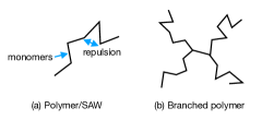
Figure 8: Polymers and branched polymers.

Our interest here will be the problem of branched polymers. Branched polymers consist of several linear polymer chains arbitrarily joined at vertices (Fig. 8(b)). They also show critical behavior in the limit of many monomers, which is different from SAW. Two commonly considered critical exponents are $\theta$ and $\nu$ which are related to the total statistical weight and to the mean size of branched polymers consisting of $N$ monomers:

$$Z_{N} \sim \mu^{N}N^{-\theta},$$ (153)

$$R_{N} \sim N^{\nu}.$$ (154)

The constant $\mu$ depends on the details of the microscopic model, but $\theta$ and $\nu$ are universal. On the lattice, branched polymers can be modeled as arbitrary connected configurations of $N$ bonds, assigning to each configuration weight 1. One may impose or not the tree topology (it turns out that the universality class does not depend on that). Such configurations are also called lattice animals. $Z_{N}$ is then the total number of lattice animals made of $N$ bonds. Lattice animals may be efficiently simulated on the lattice, and high quality determinations of $\theta,\nu$ are available in any $2\leqslant d\leqslant 8$ (which turns out to be the upper critical dimension) Hsu2005 .

We are interested in branched polymers (BP), because field theory for their statistics turns out to be closely related to RFIM. This is surprising since the problem is clearly quite different - it is purely geometric and there is no disorder. The link was found by Parisi and Sourlas PhysRevLett.46.871 , following the work by Lubensky and Isaacson PhysRevA.20.2130 . They argued that BP can be studied via the $n\rightarrow 0$ limit of the replicated action $\mathcal{S}_{n}$ (91) where $V(\phi)$ is not the quartic potential as for the RFIM, but the cubic potential with an imaginary coupling:

$$V(\phi)=\frac{1}{2}m^{2}\phi^{2}+i\frac{\lambda}{3!}\phi^{3}.$$ (155)

Then, using PS SUSY, they argued for the dimensional reduction - that the critical exponents of BP in $d$ dimensions should be the same as those for the Lee-Yang (LY) universality class in $\hat{d}=d-2$ dimensions. Recall that the LY universality class is realized by the Ising model in a critical imaginary magnetic field, and is described field-theoretically by the $i\varphi^{3}$ model - a single scalar field $\varphi$ with the cubic potential (155). LY critical exponents are well known due to the $\varepsilon$-expansion in $\hat{d}=6-\varepsilon$ dimensions, as well as exact results in $\hat{d}=0,1,2$. In this case it turns out that dimensional reduction works perfectly - BP_d and LY${}_{\hat{d}}$ exponents do agree in any $d$ Hsu2005 .

Why is the situation here so different from RFIM? Unfortunately, concerning this question there is some confusion in the literature, related to the rigorous work by Brydges and Imbrie zbMATH02068689 . This work considered a particular type of branched polymers where the distance $r$ between vertices joined by a monomer is not fixed but is distributed according to a weight $Q(r)$. Another weight $P(r)=e^{-V(r)}$, where $V(r)$ is the repulsing potential, does not allow vertices not joined by a monomer to come close to each other. A physically reasonable model requires $P(r)$ growing monotonically from $0$ at  $r\lesssim 1$ to $1$ at $r\gtrsim 1$, and $Q(r)$ peaked at $r\sim 1$. In a general model of this kind $P$ and $Q$ would be independent, but zbMATH02068689 imposes on them the special relation

$$Q(r)=P^{\prime}(r),$$ (156)

which is consistent with physical requirements. The main observation of zbMATH02068689 is that BP satisfying this relation have exact SUSY - their partition function allows an exact fermionic-integral representation. Furthermore, this SUSY representation can be shown to reduce to a grand-canonical partition function of a $\hat{d}$-dimensional gas of particles with pairwise potential $V(r)$, at negative fugacity. The latter model has, by physics arguments, a critical point in the same universality class as LY.

The result of zbMATH02068689 is sometimes quoted by saying that they proved dimensional reduction for BP, but this is misleading. They proved dimensional reduction for a particular class of models having built-in SUSY. This should not be so surprising, since we know that dimensional reduction is a consequence of SUSY. The main challenge is to show how SUSY may emerge in a model of BP which has no SUSY built in from the start, like for a model of lattice animals. However, the theorem of Brydges-Imbrie does not answer this question. For example, is their result stable with respect to small perturbations violating the relation (156)? From the mathematical point of view, this is an open problem.

From the physics perspective, stability of the SUSY fixed point of BP can be studied in the same way as for the RFIM. Namely, one does the Cardy transform of the replicated action, goes to the fixed point of the pre-SUSY action, and studies the anomalous dimensions of leaders of singlet perturbations. This was carried out by Kaviraj and Trevisani paper3 . Unlike for the RFIM, they did not find any leader interactions with negative anomalous dimensions - all additional interactions for BP seem to remain irrelevant for any $d$. This, then, is an explanation of why dimensional reduction is valid for BP in any $d$, and not only for $d>d_{c}$ as for RFIM .

Another confusion about BP is related to the question to what extent the theory is conformally invariant. This goes back to the observation of Miller and De’Bell Miller:1992uv that the critical point of BP in 2d cannot have Virasoro symmetry. Ref. Miller:1992uv looked at the free Parisi-Sourlas action, which integrating out $\omega$ has a higher-derivative in $\varphi$ piece

$$\int(\partial^{2}\varphi)^{2}d^{d}x.$$ (157)

It is indeed well known that such a Gaussian theory is not Virasoro invariant. However it is invariant under global conformal transformations (Möbius transformations). This is nontrivial and should be kept in mind. In general, the BP fixed point has global conformal invariance in any $d\geqslant 2$.

4.3 Nonperturbative RG studies of RFIM

Tarjus, Tissier and their collaborators published since 2004 Tarjus2004 many papers devoted to applying non-perturbative RG techniques to the RFIM. Their method is also known as “functional RG” (FRG) and is based on the Wetterich equation. For the $\varphi^{4}$ model (pure Ising) in $2\leqslant d\leqslant 4$, modern FRG calculations give reliable results in agreement with the $\varepsilon$-expansion and the conformal bootstrap. It is thus interesting to know what they give for the RFIM, and to compare with our results.

Ref. Tarjus2004 applied FRG to the replicated action and reported a change of the regime of the fixed point for $d<d_{c}\approx 5.1$. They associated this change with the loss of analyticity of the effective action (“cusps”), and observed that $\eta\neq\bar{\eta}$ for $d<d_{c\text{{\it}}}$, as a sign that SUSY gets broken.

It is premature to discuss the numerical difference between our and their estimate of $d_{c}$. Our scheme may be improved by including more perturbative orders, while their scheme may be improved by including more terms in the derivative expansion of the effective action. One would have to see first how $d_{c}$ changes after such improvements.

It is interesting to compare what happens at and near $d_{c}$. FRG studies find, similarly to us, two interactions heading towards the marginality threshold as $d\rightarrow d^{+}_{c}$ (see Balog:2020sre , Fig.1). There is however a qualitative difference in the predicted behavior near $d_{c}$. Ref. Balog:2020sre found a square-root behavior $\sim\sqrt{d-d_{c}}$ in the scaling dimensions. Such a square root behavior is a hallmark of fixed-point annihilation (see e.g. Gorbenko:2018ncu for a recent discussion). To cite Ref. Balog:2020sre : “What is found within the NP-FRG is that the SUSY/dimensional-reduction fixed point that controls the critical behavior of the RFIM below the upper dimension $d=6$ annihilates with another (unstable) SUSY/dimensional-reduction fixed point when $d=d_{\textit{DR}}$.”

We find this scenario problematic from several points of view. First, there is no known candidate for the unstable SUSY/dimensional-reduction fixed point. This fixed point would dimensionally reduce to an unstable non-SUSY fixed point in $3.1<d<4$ having $\mathbb{Z}_{2}$ global symmetry and there is no known fixed point with such properties.

Second, when fixed points annihilate, they usually go to the complex plane, and no real fixed points are left Gorbenko:2018ncu . Here instead at $d<5.1$ a SUSY-breaking fixed point is supposed to exist.

In our scenario, these problems are avoided because the interactions becoming marginal, $\mathcal{F}_{4}$ and $\mathcal{F}_{6}$, have susy-null and non-susy-writable leaders, i.e. belong to different symmetry classes from the susy-writable interactions present in the SUSY actions. There is no fixed point annihilation, which only happens when the marginal interaction has all symmetries of the fixed point action (i.e. is a full singlet). Instead, we have a more conventional exchange of stability between the two fixed points - SUSY for $d>d_{c}$ and non-SUSY for $d<d_{c}$.

There should be a way to distinguish the two scenarios by numerical simulations in $d=4$ dimensions. Tarjus, Tissier et al predict that the SUSY fixed point does not exist in $d=4$, having disappeared via annihilation. We predict instead that the SUSY fixed point does exist even in $d=4$, although it is unstable. Unstable fixed points may still be realized via additional tuning, as we discuss in the next section.

Further aspects of the work of Tarjus, Tissier et al are discussed in paper2 , Apps. A.7, A.8.

4.4 Tuning to the SUSY fixed point

Let’s suppose that our theory is true: for $d$ below a critical value, the interactions $\mathcal{O}_{1}=(\mathcal{F}_{4})_{L}$ and $\mathcal{O}_{2}=(\mathcal{F}_{6})_{L}$ become relevant. Consider the effective action including these terms:

$$S_{\text{eff}}=S_{\text{pre-SUSY}}+g_{1}\mathcal{O}_{1}+g_{2}\mathcal{O}_{2}.$$ (158)

Suppose that we somehow managed to tune the couplings $g_{1}$, $g_{2}$ to zero. Then, we will be left with $S_{\text{pre-SUSY}}$. In $d=4$, the pre-SUSY action flows for a particular value of the mass to a SUSY fixed point, which should dimensionally reduce to the critical 2d Ising model. In $d=3$, the pre-SUSY action flows to a gapped phase for any value of the mass (this is related to the fact that the $d=1$ $\varphi^{4}$ theory is gapped for any value of the mass). Thus, we may hope to realize the SUSY fixed point in $d=4$ (but not in $d=3$) by tuning. This was proposed in paper2 ; paper-summary as a smoking gun for our scenario, allowing to distinguish it from other scenarios such as the work of Tarjus, Tissier et al, Section 4.3.

Let us first discuss the pattern of renormalization group flows and fixed points which arises when couplings $g_{1}$ and $g_{2}$ become relevant. Then, we will discuss various scenarios of what may happen when the microscopic theory is tuned. We will see that it is actually sufficient to tune one of the two couplings to zero to observe SUSY.

We will be very schematic. We may describe the RG flow of $g_{1},g_{2}$ by the following approximate beta-functions:

$$\frac{dg_{1}}{d\log a} = A_{1}(d_{c1}-d)g_{1}-B_{1}g_{1}^{2},$$ (159)

$$\frac{dg_{2}}{d\log a} = A_{2}(d_{c2}-d)g_{2}-B_{2}g_{2}^{2}.$$

The coefficients $A_{i}$ are positive, so that $g_{i}$ is relevant (grows towards IR) for $d<d_{ci}$, $i=1,2$. We will continue to assume that $d_{c1}$ is slightly larger than $d_{c2}$, as Section 3.8 indicates. The coefficient $B_{i}$ is proportional to the coefficient with $\mathcal{O}_{i}$ appears in the OPE $\mathcal{O}_{i}\times\mathcal{O}_{i}$. A computation in $d=6$ using the expression for $\mathcal{O}_{i}$ from Section 3.7 gives $B_{1},B_{2}>0$. We will assume that the sign of $B_{i}$ does not change between $d=6$ and $d=d_{ci}$. We could add a term $Cg_{2}$ to the first beta-function, showing that $g_{2}$ can generate $g_{1}$ (while the opposite process is forbidden by the selection rules). This term does not influence much the discussion below, and we will set $C=0$.

For $d_{c2}<d<d_{c1}$, the coupling $g_{2}$ is irrelevant and $g_{1}$ is relevant. For negative initial values, $g_{1}$ flows towards $-\infty$. If this situation is indeed realized, then SUSY may be broken already at $d=d_{c1}$. This is because a large susy-null coupling may give large corrections to anomalous dimensions of non-susy-writable couplings, which may become relevant and break SUSY. This answers the question from Section 3.7 why one should worry about susy-null interactions.

On the other hand, when $g_{1}$ has a positive initial value, it flows to a stable fixed point $g^{\ast}_{1}=A_{1}(d_{c1}-d)/B_{1}$. Since $\mathcal{O}_{1}$ is a susy-null interaction, all susy-writable observables are not modified. We do expect corrections to non-susy-writable observables, e.g. dimensions of nsw interactions. These corrections will be small since $d$ is close to $d_{c1}$ and $g^{\ast}_{1}$ is small. It is very hard to distinguish this fixed point from the one having $g_{1}=0$. Both fixed points are SUSY and have the same values of the main critical exponents $\nu,\eta,\bar{\eta}$. Thus, in this case, SUSY does not get broken at $d=d_{c1}$.

As we lower $d$ further, $d<d_{c2}$, coupling $g_{2}$ also becomes relevant. The SUSY fixed point at $g_{2}=0$ becomes unstable, and a stable non-SUSY fixed point appears at $g^{\ast}_{2}=A_{2}(d_{c2}-d)/B_{2}>0$. For the initial $g_{2}$ positive, the flow will be attracted to the stable fixed point. For the initial $g_{2}$ negative, the flow goes towards large negative couplings and its fate is uncertain. It may lead to a first order phase transition or to another non-SUSY fixed point not visible in this approximation.

We note in passing that for $d>d_{c2}$ the beta-functions predict a stable fixed point at $g_{2}=0$ and an unstable fixed point at $g_{2}<0$. The status of the latter fixed point is unclear - it may be invalidated by non-perturbative effects similarly to how the Wilson-Fisher fixed point at $d>4$ is destroyed by non-perturbative instability of the $\lambda\varphi^{4}$ potential with negative coupling.

Analogously for $d>d_{c1}$ the beta-functions predict a stable SUSY fixed point at $g_{1}=0,g_{2}=0$ and an unstable SUSY fixed point at $g_{1}<0,g_{2}=0$. From the susy-writable sector perspective, it’s the same fixed point. That’s why this discussion does not contradict what we said in Section 4.3 - that there is no known second SUSY fixed point at $d>d_{c}$, substantially (i.e. in the SUSY sector) different from the one we are discussing, and which could annihilate with it.

Coming back to $d<d_{c2}$, the full RG flow diagram is shown in Fig 9. We see two SUSY fixed points I and II, and two non-SUSY fixed points III and IV. The fixed points I and II are, as discussed, identical as far as the susy-writable observables are concerned; they have the same $\nu$ and $\eta=\bar{\eta}$ and have dimensional reduction. The fixed points III and IV have $\nu$, $\eta,\bar{\eta}$ different from each other and from I,II; they are not expected to obey $\eta=\bar{\eta}$ nor dimensional reduction. The fixed point IV is the most stable one, the first quadrant being its basin of attraction. It is the prime candidate for describing the RFIM phase transition in $d=4$.

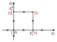
Figure 9: Pattern of fixed points and RG flows for $d<d_{c2}$.

What does this imply about the prospects of observing SUSY in a tuned numerical simulation? In numerical simulations we first choose the shape of the random magnetic field distribution $P[h]$. We then pick a parameter $\kappa>0$ playing the role of the strength of the random magnetic field. We sample the rescaled distribution

$$P_{\kappa}[h]=\frac{1}{\kappa}P[h/\kappa].$$ (160)

For some $\kappa=\kappa_{c}$, depending on $P[h]$, a phase transition is realized.

In Section 1.4 we fixed $P[h]$ to be a Gaussian, but this does not have to be the case. When we vary $P[h]$ in the microscopic theory, this translates into varying couplings $g_{1},g_{2}$ in the effective field theory description (158) of the phase transition. For example, we may consider a one-parameter family interpolating between the Gaussian distribution with variance 1, and the bimodal distribution $\frac{1}{2}[\delta(h-1)+\delta(h+1)]$.

Any such family will trace a curve of initial conditions in the RG flow diagram of Fig. 9. We don’t a priori know how this curve will pass. Let us consider a couple of examples. In Fig. 10 we have a favorable situation for the observation of SUSY. The curve of initial conditions, parameterized by $t\in[0,1]$, exits the basin of attraction of fixed point IV at $t=t_{0}$ crossing the axis $g_{2}=0$ at $g_{1}>0$, which gets attracted to the SUSY fixed point II. For $t>t_{0}$ we have $g_{2}$ flowing to negative values, which may lead to a first-order transition or another fixed point not visible in our treatment.

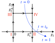
Figure 10: One parameter family of initial conditions where SUSY may be observed at $t=t_{0}$.

In Fig. 11 the situation is not so rosy - SUSY does not reveal itself. We will observe the non-SUSY fixed point IV for $t<t_{0}$, and another fixed point III at $t=t_{0}$ which is also not SUSY. For $t>t_{0}$ the flow leads to large negative values of $g_{1}$ and/or $g_{2}$ and is not under control. The $g_{2}=0$ line is crossed at $g_{1}<0$, which does not get attracted to a SUSY fixed point.

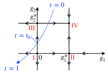
Figure 11: One parameter family of initial conditions where SUSY will not be observed.

The punchline of this discussion is that one may hope to see a SUSY fixed point even for a one-parameter family of initial conditions, but one needs a bit of luck and/or experimentation to find a family crossing $g_{2}=0$ line at $g_{1}>0$.

We note that Refs. Fytas3 ; Picco1 did already consider varying the random magnetic field distribution. In $d=3$, Ref. Fytas3 considered distributions along the Gaussian-bimodal interpolating family mentioned above, as well as the Poissonian distribution. They did not see any evidence for the SUSY fixed points - all distributions led to the same, non-SUSY, critical exponents (albeit the distributions close to the bimodal one had large corrections to scaling). This is consistent with our remarks above, that a SUSY fixed point is expected to exist in $d=4$ but not in $d=3$.

In $d=4$, Ref. Picco1 considered only the Gaussian and the Poissonian distributions, which led to the same, non-SUSY, critical exponents. It would be very interesting to carry out a $d=4$ study for more distributions and look for changes in exponents. In the meantime, motivated by paper2 , an ongoing $d=4$ study by the authors of Picco3 along the Gaussian-bimodal family is showing intriguing preliminary results: a new fixed point close to the bimodal distribution (where the $d=3$ study saw large corrections to scaling). Hopefully, it will be soon clarified if this fixed point obeys dimensional reduction and supersymmetry.

References

- (1) Y. Imry and S.-k. Ma, “Random-Field Instability of the Ordered State of Continuous Symmetry,” Phys. Rev. Lett. 35 (1975) 1399–1401.
- (2) A. Aharony, Y. Imry, and S. K. Ma, “Lowering of Dimensionality in Phase Transitions with Random Fields,” Phys. Rev. Lett. 37 (1976) 1364–1367.
- (3) G. Parisi and N. Sourlas, “Random Magnetic Fields, Supersymmetry and Negative Dimensions,” Phys. Rev. Lett. 43 (1979) 744.
- (4) E. Brézin and C. De Dominicis, “New phenomena in the random field Ising model,” Europhys Lett. 44 no. 1, (1998) 13–19, cond-mat/9804266.
- (5) D. E. Feldman, “Critical Exponents of the Random-Field Model,” Phys. Rev. Lett. 88 (2002) 177202, arXiv:cond-mat/0010012 [cond-mat.dis-nn].
- (6) G. Tarjus and M. Tissier, “Nonperturbative Functional Renormalization Group for Random-Field Models: The Way Out of Dimensional Reduction,” Phys. Rev. Lett. 93 no. 26, (2004) 267008, arXiv:cond-mat/0410118 [cond-mat.dis-nn].
- (7) D. Belanger and A. Young, “The random field ising model,” J. Magn. Magn. Mater. 100 no. 1, (1991) 272 – 291.
- (8) N. G. Fytas, V. Martín-Mayor, M. Picco, and N. Sourlas, “Phase Transitions in Disordered Systems: The Example of the Random-Field Ising Model in Four Dimensions,” Phys. Rev. Lett. 116 (2016) 227201, arXiv:1605.05072 [cond-mat.dis-nn].
- (9) N. G. Fytas, V. Martín-Mayor, M. Picco, and N. Sourlas, “Restoration of dimensional reduction in the random-field Ising model at five dimensions,” Phys. Rev. E 95 (2017) 042117, arXiv:1612.06156 [cond-mat.dis-nn].
- (10) N. G. Fytas, V. Martín-Mayor, G. Parisi, M. Picco, and N. Sourlas, “Evidence for Supersymmetry in the Random-Field Ising Model at ,” Phys. Rev. Lett. 122 (2019) 240603, arXiv:1901.08473 [cond-mat.stat-mech].
- (11) A. Kaviraj, S. Rychkov, and E. Trevisani, “Random Field Ising Model and Parisi-Sourlas supersymmetry. Part I. Supersymmetric CFT,” JHEP 04 (2020) 090, arXiv:1912.01617 [hep-th].
- (12) A. Kaviraj, S. Rychkov, and E. Trevisani, “Random field Ising model and Parisi-Sourlas supersymmetry. Part II. Renormalization group,” JHEP 03 (2021) 219, arXiv:2009.10087 [cond-mat.stat-mech].
- (13) A. Kaviraj, S. Rychkov, and E. Trevisani, “Parisi-Sourlas Supersymmetry in Random Field Models,” Phys. Rev. Lett. 129 no. 4, (2022) 045701, arXiv:2112.06942 [cond-mat.stat-mech].
- (14) A. Kaviraj and E. Trevisani, “Random field model and Parisi-Sourlas supersymmetry,” JHEP 08 (2022) 290, arXiv:2203.12629 [hep-th].
- (15) J. L. Cardy, Scaling and renormalization in statistical physics. Cambridge, UK: Univ. Pr., 238 p., 1996.
- (16) A. J. Bray and M. A. Moore, “Scaling theory of the random-field Ising model,” J. of Phys. C 18 no. 28, (1985) L927–L933.
- (17) J. Z. Imbrie, “The ground state of the three-dimensional random-field ising model,” Comm. Math. Phys. 98 no. 2, (1985) 145–176.
- (18) J. Bricmont and A. Kupiainen, “Phase transition in the 3d random field Ising model,” Comm. Math. Phys. 116 no. 4, (1988) 539–572.
- (19) J. Ding and Z. Zhuang, “Long range order for random field Ising and Potts models,” arXiv:2110.04531 [math.PR].
- (20) J. Ding, Y. Liu, and A. Xia, “Long range order for three-dimensional random field Ising model throughout the entire low temperature regime,” arXiv:2209.13998 [math.PR].
- (21) M. Aizenman and J. Wehr, “Rounding effects of quenched randomness on first-order phase transitions,” Comm. Math. Phys. 130 no. 3, (1990) 489–528.
- (22) J. Ding and J. Xia, “Exponential decay of correlations in the two-dimensional random field Ising model,” arXiv:1905.05651 [math.PR].
- (23) D. P. Belanger, “Experiments on the Random Field Ising Model,” in Spin Glasses And Random Fields, A. P. Young, ed., pp. 251–275. World Scientific, 1997. arXiv:cond-mat/9706042 [cond-mat.dis-nn].
- (24) S. Fishman and A. Aharony, “Random field effects in disordered anisotropic antiferromagnets,” J. of Phys. C 12 no. 18, (1979) L729.
- (25) J. L. Cardy, “Random-field effects in site-disordered ising antiferromagnets,” Phys. Rev. B 29 (1984) 505–507.
- (26) J. Rong, “Scalar CFTs from structural phase transitions,” arXiv:2303.12028 [hep-th].
- (27) G. A. Gehring and K. A. Gehring, “Co-operative jahn-teller effects,” Reports on Progress in Physics 38 no. 1, (1975) 1.
- (28) J. T. Graham, M. Maliepaard, J. H. Page, S. R. P. Smith, and D. R. Taylor, “Random-field effects on Ising Jahn-Teller phase transitions,” Phys. Rev. B 35 (1987) 2098–2101.
- (29) P. G. de Gennes, “Liquid-liquid demixing inside a rigid network. qualitative features,” J. Phys. Chem. 88 no. 26, (1984) 6469–6472.
- (30) S. K. Sinha, J. Huang, and S. K. Satija, “Binary fluid phase separation in gels: A neutron scattering study,” in Scaling Phenomena in Disordered Systems, R. Pynn and A. Skjeltorp, eds., pp. 157–162. Springer (Boston), 1991.
- (31) M. Alava, P. Duxbury, C. Moukarzel, and H. Rieger, “Exact combinatorial algorithms: Ground states of disordered systems,” in Phase Transitions and Critical Phenomena, vol. 18, C. Domb and J. Lebowitz, eds., pp. 143–317. Academic Press, 2001.
- (32) N. G. Fytas and V. Martín-Mayor, “Efficient numerical methods for the random-field Ising model: Finite-size scaling, reweighting extrapolation, and computation of response functions,” Phys. Rev. E 93 no. 6, (2016) 063308, arXiv:1512.06571 [cond-mat.dis-nn].
- (33) N. G. Fytas and V. Martín-Mayor, “Universality in the Three-Dimensional Random-Field Ising Model,” Phys. Rev. Lett. 110 no. 22, (2013) 227201, arXiv:1304.0318 [cond-mat.dis-nn].
- (34) F. Kos, D. Poland, D. Simmons-Duffin, and A. Vichi, “Precision Islands in the Ising and Models,” JHEP 08 (2016) 036, arXiv:1603.04436 [hep-th].
- (35) F. Wegner, Supermathematics and its Applications in Statistical Physics: Grassmann Variables and the Method of Supersymmetry, vol. 920. Springer, 2016.
- (36) J. L. Cardy, “Nonperturbative effects in a scalar supersymmetric theory,” Physics Letters B 125 no. 6, (1983) 470 – 472.
- (37) O. V. Zaboronski, “Dimensional reduction in supersymmetric field theories,” Journal of Physics A: Mathematical and General 35 no. 26, (2002) 5511–5519, arXiv:hep-th/9611157 [hep-th].
- (38) S. Cremonesi, “An Introduction to Localisation and Supersymmetry in Curved Space,” PoS Modave2013 (2013) 002.
- (39) G. Parisi, “An introduction to the statistical mechanics of amorphous systems,” in Recent Advances in Field Theory and Statistical Mechanics, Proceedings of Les Houches 1982, Session XXXIX, J. B. Zuber and R. Stora, eds., p. 473. North-Holland, Amsterdam, 1984. Reprinted in G. Parisi, “Field Theory, Disorder and Simulations”, World Scientific, 1992.
- (40) S. Rychkov, “Random magnetic fields, supersymmetry, and negative dimensions.”. Talk in the series “The interdisciplinary contribution of Giorgio Parisi to theoretical physics”, La Sapienza University, Rome, Italy, 2.2.2023.
- (41) J. Cardy, Scaling and Renormalization in Statistical Physics. Cambridge Lecture Notes in Physics. Cambridge University Press, 1996.
- (42) J. L. Cardy, “Nonperturbative aspects of supersymmetry in statistical mechanics,” Physica D: Nonlinear Phenomena 15 no. 1, (1985) 123 – 128.
- (43) C. De Dominicis and I. Giardina, Random Fields and Spin Glasses: A Field Theory Approach. Cambridge University Press, 2006.
- (44) A. Pelissetto and E. Vicari, “Critical phenomena and renormalization-group theory,” Phys. Rept. 368 (2002) 549–727, arXiv:cond-mat/0012164.
- (45) S. M. Chester, W. Landry, J. Liu, D. Poland, D. Simmons-Duffin, N. Su, and A. Vichi, “Bootstrapping Heisenberg magnets and their cubic instability,” Phys. Rev. D 104 no. 10, (2021) 105013, arXiv:2011.14647 [hep-th].
- (46) M. Hasenbusch, “Cubic fixed point in three dimensions: Monte Carlo simulations of the 4 model on the simple cubic lattice,” Phys. Rev. B 107 no. 2, (2023) 024409, arXiv:2211.16170 [cond-mat.stat-mech].
- (47) G. Badel, G. Cuomo, A. Monin, and R. Rattazzi, “The Epsilon Expansion Meets Semiclassics,” JHEP 11 (2019) 110, arXiv:1909.01269 [hep-th].
- (48) M. E. Peskin and D. V. Schroeder, An Introduction to quantum field theory. Addison-Wesley, Reading, USA, 1995.
- (49) A. Vasil’ev, The Field Theoretic Renormalization Group in Critical Behavior Theory and Stochastic Dynamics. CRC Press LLC, 2020.
- (50) J. Zinn-Justin, “Quantum field theory and critical phenomena,” Int. Ser. Monogr. Phys. 113 (2002) 1–1054.
- (51) H. Kleinert and V. Schulte-Frohlinde, Critical properties of theories. World Scientiic, 2001.
- (52) G. P. Korchemsky, “On level crossing in conformal field theories,” JHEP 03 (2016) 212, arXiv:1512.05362 [hep-th].
- (53) C. Behan, “Conformal manifolds: ODEs from OPEs,” JHEP 03 (2018) 127, arXiv:1709.03967 [hep-th].
- (54) J. Henriksson, S. R. Kousvos, and M. Reehorst, “Spectrum continuity and level repulsion: the Ising CFT from infinitesimal to finite ,” JHEP 02 (2023) 218, arXiv:2207.10118 [hep-th].
- (55) H.-P. Hsu, W. Nadler, and P. Grassberger, “Simulations of lattice animals and trees,” J. Phys. A 38 no. 4, (2005) 775–806, arXiv:cond-mat/0408061 [cond-mat.stat-mech].
- (56) G. Parisi and N. Sourlas, “Critical Behavior of Branched Polymers and the Lee-Yang Edge Singularity,” Phys. Rev. Lett. 46 (1981) 871–874.
- (57) T. C. Lubensky and J. Isaacson, “Statistics of lattice animals and dilute branched polymers,” Phys. Rev. A 20 (1979) 2130–2146.
- (58) D. C. Brydges and J. Z. Imbrie, “Branched polymers and dimensional reduction.,” Ann. Math. 158 no. 3, (2003) 1019–1039, arXiv:math-ph/0107005.
- (59) J. D. Miller and K. De’Bell, “Randomly branched polymers and conformal invariance,” arXiv:hep-th/9211127.
- (60) J. Polchinski, “Scale and Conformal Invariance in Quantum Field Theory,” Nucl. Phys. B 303 (1988) 226–236.
- (61) I. Balog, G. Tarjus, and M. Tissier, “Dimensional reduction breakdown and correction to scaling in the random-field Ising model,” Phys. Rev. E 102 (2020) 062154, arXiv:2008.13650 [cond-mat.dis-nn].
- (62) V. Gorbenko, S. Rychkov, and B. Zan, “Walking, Weak first-order transitions, and Complex CFTs,” JHEP 10 (2018) 108, arXiv:1807.11512 [hep-th].
- (63) K. J. Wiese, “Theory and experiments for disordered elastic manifolds, depinning, avalanches, and sandpiles,” Rept. Prog. Phys. 85 no. 8, (2022) 086502, arXiv:2102.01215 [cond-mat.dis-nn].
- (64) S. Rychkov, “Random Field Ising Model and Parisi-Sourlas Supersymmetry - some recent developments.”. Mathematics Meets Physics on Disordered Systems, PhD School, Cortona, Italy, April 25-May 6, 2022.
- (65) S. Rychkov, “The fate of Parisi-Sourlas supersymmetry in random-field models.”. Conformal field theory and quantum many-body physics, August 22 - September 9, 2022, Centre de Recherches Mathematiques, Université de Montréal, Quebec, Canada.
- (66) S. Rychkov, “Random Field Ising Model and Parisi-Sourlas Supersymmetry.”. Lectures at the Institut des Hautes Études Scientifiques, Nov. 2022.