Iterative Soft Shrinkage Learning for Efficient Image Super-Resolution

Abstract

Image super-resolution (SR) has witnessed extensive neural network designs from CNN to transformer architectures. However, prevailing SR models suffer from prohibitive memory footprint and intensive computations, which limits further deployment on edge devices. This work investigates the potential of network pruning for super-resolution to take advantage of off-the-shelf network designs and reduce the underlying computational overhead. Two main challenges remain in applying pruning methods for SR. First, the widely-used filter pruning technique reflects limited granularity and restricted adaptability to diverse network structures. Second, existing pruning methods generally operate upon a pre-trained network for the sparse structure determination, hard to get rid of dense model training in the traditional SR paradigm. To address these challenges, we adopt unstructured pruning with sparse models directly trained from scratch. Specifically, we propose a novel Iterative Soft Shrinkage-Percentage (ISS-P) method by optimizing the sparse structure of a randomly initialized network at each iteration and tweaking unimportant weights with a small amount proportional to the magnitude scale on-the-fly. We observe that the proposed ISS-P can dynamically learn sparse structures adapting to the optimization process and preserve the sparse model’s trainability by yielding a more regularized gradient throughput. Experiments on benchmark datasets demonstrate the effectiveness of the proposed ISS-P over diverse network architectures. Code is available at https://github.com/Jiamian-Wang/Iterative-Soft-Shrinkage-SR

1 Introduction

Single image super-resolution [18, 20] aims to reconstruct the high-resolution (HR) image from a low-resolution (LR) input. Towards a high-fidelity reconstruction, research efforts have been made by relying on the strong modeling capacity of convolutional neural networks [7, 19, 26, 47]. More recently, advanced Transformer architectures [25, 45, 50] are elaborated, enabling photorealistic restoration. Despite the impressive performance, the excessive memory footprint of existing models has been de facto in the field, which inevitably prohibits the deployment of advanced SR models on computational-constrained devices.

To alleviate the computational complexity, we study network pruning, which takes advantage of off-the-shelf advanced network architectures to realize efficient yet accurate SR models. Network pruning has been long developed in two mainstream directions. On the one hand, filter pruning (structured pruning) [23] cuts off the specific filter of convolutional layers, among which representative practices in SR is to prune cross-layer filters governed by residual connections [48, 49]. However, these methods need to consider the layer-wise topology by posing structural constraints, requiring a heuristic design and thus making them inflexible. Plus, filter pruning inhibits a more fine-grained manipulation to the network. On the other hand, weight pruning (unstructured pruning) directly removes weight scalars across the network, endowed with more flexibility by accommodating weight discrepancy. Also, the weight pruning method allows a very high pruning ratio, e.g., a ratio of $99\%$ with competitive performance [10, 11]. To this end, this work focuses on delivering a highly-adaptive unstructured pruning solution for diverse SR architectures.

Generally, pruning algorithms are widely recognized to have three steps: (1) pre-training, (2) sparse structure acquisition, and (3) fine-tuning the sparse network. Among these steps, the dense network pre-training usually introduces heavy costs beyond the sparse network optimization. For example, before obtaining a sparse network, the CAT [50] network architecture takes $2$ days to train its dense counterpart on $4$ A100 GPUs. Thus, a natural question arises to save training time further – can we directly explore the sparsity of network structures from random initialization?

We start from the baseline method by performing random pruning on weights at initialization, whose limitation is the irrelevance between the sparse structure and the weight distribution varying to the optimization. Following this line, we apply the widely-used $L_{1}$ norm [23, 11] pruning on randomly initialized weights. However, the immutable sparsity cannot be well aligned with the optimization, leading to limited performance. To tackle this problem, we introduce an iterative hard thresholding [4, 5] method (IHT) stemming from compressive sensing [6, 8], where the iterative gradient descent step is regularized by a hard thresholding function. Unlike previous works, we tailor IHT to iteratively set unimportant weights as zeros and preserve the important weight magnitudes. By this means, the sparse structure adapts to the weight distribution throughout the training, which potentially better selects essential weights. However, the sparse structure alignment in IHT is heavily susceptible to the magnitude-gradient relationship. The zeroed weight can be continually trapped as “unimportant” once the scales of magnitude and gradient are incomparable. Moreover, by directly zeroing out unimportant weights, IHT blocks the error back-propagation at each iteration, especially hindering the optimization in shallow layers.

To address the aforementioned negative effects, we introduce a more flexible thresholding function for an expressive treatment of unimportant weights. A natural tuning approach is to softly shrink the weights rather than hard threshold. We first explore the soft shrinkage by a growing regularization method [49], namely ISS-R. Per each iteration, the proposed ISS-R constrains weight magnitudes with a gradually increasing weighted $L_{2}$ regularization, to avoid the conflict between network pruning and smooth sparse network optimization. However, the growing regularization schedule involves a number of hyperparameter tuning, requiring cumbersome manual efforts. Notably, the $L_{2}$ regularization shrinkage inside ISS-R is, in essence, proportional to the weight magnitude. Based on this insight, we propose a new iterative soft shrinkage function to simplify the regularization by equivalently shrinking the weight with a percentage (ISS-P). It turns out that ISS-P not only encourages dynamic network sparsity, but also preserves the sparse network trainability, resulting in better convergence. We summarize the contributions of this work as follows:

• We introduce a novel unstructured pruning method, namely iterative soft shrinkage-percentage (ISS-P), which is compatible with diverse SR network designs. Unlike existing pruning strategies for SR, the proposed method trains the sparse network from scratch, providing a practical solution for sparse network acquisition under computational budget constraints.

• We explore pruning behaviors by interpreting the trainability of sparse networks. The proposed ISS-P enjoys a more promising gradient convergence and enables dynamic sparse structures in the training process, offering new insights to design pruning methods for SR.

• Extensive experimental results on benchmark testing datasets at different pruning ratios and scales demonstrate the effectiveness of the proposed method compared with state-of-the-art pruning solutions.

2 Related Work

Single Image Super-Resolution. The task of single image super-resolution has been developed with remarkable progress since the first convolutional network of SRCNN [7] was introduced. By taking advantage of the residual structure [12], VDSR [19] further encourages fine-grained reconstruction at rich textured areas. Based on it, EDSR [26] witnessed a promotion by empowering the regression with deeper network depth and a simplified structure. Besides, RCAN [47] outperforms its counterparts by incorporating channel attention into the residual structure. HPUN [36] proposes a downsampling module for a efficient modeling. More recently, transformer [9, 39] has become a prevailing option due to its long-range dependency modeling capacity. SwinIR [25] equips attention with spatial locality and translation invariance properties. Another design of CAT [50] exploiting the power of the transformer by developing a flexible window interaction. However, advanced SR models are characterized by rising computational overhead and growing storage costs.

Neural Network Pruning in SR. Neural network pruning [33, 37] compresses and accelerates the network by removing redundant parameters. It has been developed in two categories: (1) Structured pruning, which mainly refers to the filter pruning [13, 14, 15, 22, 23, 24, 27, 44], removes the redundant filters for a sparsity pattern exploitation. Recently, two novel works discussed the filter pruning specialized for SR models. ASSL [48] handles the residual network by regularizing the pruned filter locations of different layers upon an alignment penalty. GASSL [42] expands the ASSL by a Hessian-Aided Regularization. Later, SRP [49] makes a step further by simplifying the determination of pruned filter indices and yields a state-of-the-art performance. However, both of them require heuristic design for the pruning schedule, hard to extend to diverse neural architectures. (2) Unstructured pruning (weight pruning) [11] directly manipulates the weights for the sparsity determination. Despite the flexibility, there lacks an effective pruning strategy proposed to broadly handle advanced SR networks. Our work is to deliver a more generalized solution for different architectures. Besides our setting, another emerging trend is to develop fine-grained pruning upon N:M sparsity [17, 30]. Among them, SLS [31] adapts the layer-wise sparsity level upon the trade-off between the computational cost and performance for the convolutional network pruning. Yet, the effectiveness of this method toward novel neural architectures, e.g., Transformers, has not been explored.

3 Method

We give the background of SR in Section 3.1 and pruning prerequisites in Section 3.2. We then tailor the classic pruning method to SR by iterative hard thresholding (IHT) in Section 3.3. We develop our method of iterative soft shrinkage by percentage (ISS-P) in Section 3.4.

3.1 Single Image Super-resolution

The task of single image super-resolution is to restore the high-resolution (HR) image $I_{\texttt{HR}}$ upon the low-resolution (LR) counterpart $I_{\texttt{LR}}$ as $I_{\texttt{HR}}=F(\Theta;I_{\texttt{LR}})$, where $F(\cdot)$ is the SR network and $\Theta$ denotes all of the learnable parameters in the network. Given a training dataset $\mathcal{D}$, privileging practice is to formulate the SR as a pixel-wise reconstruction problem and solve it with the MSE loss by

$$J(\Theta;\mathcal{D})=\frac{1}{|\mathcal{D}|}\sum_{\mathcal{D}}||F(\Theta;I_{\texttt{LR}})-I_{\texttt{HR}})||^{2},$$ (1)

where $I_{\texttt{LR}},I_{\texttt{HR}}\in\mathcal{D}$. While existing deep SR networks have achieved an impressive photorealistic performance, their cumbersome computation inhibits further deployment on edge devices. In this work, we propose a generalized pruning method for off-the-shelf network designs. We introduce the prerequisites for pruning in the following.

3.2 Prerequisites for Pruning

Pruning Granularity. Pruning granularity refers to the basic weight group to be removed from the network. In unstructured (weight) pruning, weight scalars are taken as manipulation units, which allows different treatment toward the neighbored weights. Besides, recent SR models have been advanced with diverse operators and structures, e.g., convolution, multi-head self-attention, residual blocks, etc. Unstructured pruning can be flexibly incorporated into diverse structures without additional constraints.

Pruning Schedule. The prevailing pruning schedule is widely recognized as three steps: (1) pre-training a dense network, (2) pruning, and (3) fine-tuning the sparse network for performance compensation. However, training a dense SR network in step (1) from scratch already introduces heavy costs beyond the sparse network optimization in step (2$\sim$3). To alleviate this problem, in this work, we exploit the sparse network acquisition schedule directly from networks at random initialization and get rid of the first step.

Baseline Methods. Bearing with above considerations, we firstly apply several baseline pruning methods to randomly initialized SR networks, including 1) directly training a sparse network with a random sparse structure, namely scratch, and 2) $L_{1}$ norm pruning (dubbed as $L_{1}$-norm) [23]. These two baselines, Sctrach and $L_{1}$-norm, are widely used in mainstream pruning literature. However, they both fail to adjust the sparse structure adapting to the weight magnitude fluctuation incurred by gradient descent – initially unimportant weights with small magnitude can be finally preserved due to negligible gradient at certain iterations of backpropagation, while initially important weights (large magnitude) with prominent gradients can be eliminated.

Notations. Let $k\in K$ be the training iterations, where $K$ is consistent among different pruning methods. Pruning is conducted in a layer-wise manner in each iteration. Given a network with $L$ layers, we define $\theta^{[k]}_{l}\in\Theta$ as an arbitrary weight magnitude in the $l$-th layer at $k$-th iteration. Without losing the generality, we will present pruning by taking the $\theta^{[k]}_{l}$ as an example throughout the methodology.

3.3 Iterative Hard Thresholding

To better capture essential network weights during the optimization, we introduce an iterative hard thresholding (IHT) method in light of compressive sensing (CS) [6, 8]. Typically, IHT operates on the iterative gradient descent with a hard thresholding function, serving as a widely-used method for $L_{0}$-norm-based non-convex optimization problems [5]. Unlike the IHT practices in CS, we develop a hard thresholding function $H(\cdot)$ to adjust the weight magnitudes, which takes effect at each forward propagation by

$$\theta^{[k]}_{l}\!=\!H(\theta^{[k]}_{l})~{}~{}\textup{where}~{}~{}H(\theta^{[k]}_{l})\!=\!\begin{cases}\theta^{[k]}_{l},\textup{~{}if~{}}\theta^{[k]}_{l}\geq\tau^{[k]}_{l},\\ 0,\textup{~{}if~{}}\theta^{[k]}_{l}<\tau^{[k]}_{l},\end{cases}$$ (2)

where $\tau^{[k]}_{l}$ denotes the threshold magnitude of the $l$-th layer at $k$-th iteration, determined by an $L_{1}$-norm sorting of the $l$-th layer weights with a given pruning ratio $r$. We define pruning iterations as $K_{\texttt{p}}$, after which we freeze the sparsity pattern by exchanging $\tau^{[k]}_{l}$ with $\tau^{[K_{\texttt{p}}]}_{l}$, and continually fine-tune the model for another $K_{\texttt{FT}}$ iterations for performance compensation. Note that we have $K=K_{\texttt{p}}+K_{\texttt{FT}}$, where the total training iterations $K$ equals to the sum of pruning iterations $K_{\texttt{p}}$ and the fine-tuning ones $K_{\texttt{FT}}$. There are no modifications to the backpropagation in training.

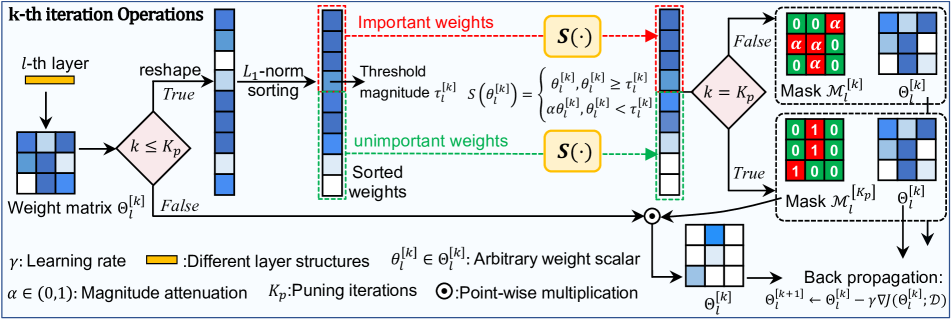
Figure 1: Training pipeline of the proposed Iterative Soft Shrinkage-Percentage (ISS-P), which is exampled by $l$-th learnable layer of the network at $k$-th training iteration. In the pruning stage ($k\leq K_{\texttt{p}}$), ISS-P selectively attenuates the unimportant weight and keeps the essential ones upon $L_{1}$-norm sorting at the forward propagation. In the fine-tuning stage ($K_{\texttt{p}}$$\leq$$k$$\leq$$K_{\texttt{p}}$$+$$K_{\texttt{FT}}$), the mask is frozen as $\mathcal{M}_{l}^{[K_{\texttt{p}}]}$ and repeatedly applied at each forward propagation. We perform a standard backpropagation in each iteration. The proposed method can flexibly prune different types of layers (i.e., convolution, linear, etc.) and directly train a sparse network from the random initialization.

Different from the static mask determination, the sparse structure of IHT changes during the optimization on-the-fly, which allocates more flexibility for fitting the optimal sparse pattern. However, several limitations still exist. The first is a network throughput blocking effect. Consider the back-propagated errors between hidden layers in a neural network, $\mathbf{\delta}_{l}=[\Theta_{l+1}^{T}\mathbf{\delta}_{l+1}]\odot\sigma^{\prime}(\mathbf{z}_{l})$, where $\mathbf{\delta}_{l}$ presents the error propagated to the $l$-th layer, $\Theta_{l+1}$ denotes the weight matrix of the $(l+1)$-th layer, and $\sigma^{\prime}(\mathbf{z}_{l})$ computes the derivative of the activation $\sigma(\cdot)$ with the hidden representation $\mathbf{z}_{l}$. Due to the iterative hard thresholding operation $H(\cdot)$, there will be a certain amount of weights becomes zero, which further suspends the error transmission to the $l$-th layer, thus hindering the update of shallow weights. Secondly, the sparse structure of the IHT is largely susceptible to the relationship between the weight magnitude and gradient. The zeroed weights are vulnerable to being trapped as the “unimportant” category when the gradient is unexpectedly large, leading to a static sparsity during the training. Additionally, the hard thresholding operator uniformly forces all the unimportant weight to be zeros, neglecting the inherent difference between the magnitudes.

3.4 Iterative Soft Shrinkage

Iterative Soft Shrinkage-Regularization (ISS-R). To address the challenges posed by the IHT, we further tailor the hard thresholding function by offering a more expressive and flexible shrinkage function toward unimportant weights, rather than solely zero-out. Accordingly, we propose a soft shrinkage function $S(\cdot)$ to facilitate the sparse network training. We first propose a regularization-driven method by introducing an $L_{2}$-norm regularization on weight magnitudes and implement a growing regularization [41, 2] schedule to encourage heterogeneity among unimportant weights, namely iterative soft shrinkage-regularization (ISS-R).

Specifically, given a network with randomly initialized weights, we perform $L_{1}$-norm sorting to the weight magnitudes for the significant weight selection. We then include the unimportant ones into the regularization and impose an $l_{2}$ penalty in the backpropagation of each iteration $k\in K_{\texttt{p}}$. Different from IHT, ISS-R naturally integrates the penalization on unimportant weights into optimization. The backpropagation of ISS-R at the pruning stage is given as

$$\theta^{[k+1]}_{l}\leftarrow\begin{cases}\theta^{[k]}_{l}-\gamma\nabla J(\theta^{[k]}_{l};\mathcal{D}),\textup{~{}if~{}}\theta^{[k]}_{l}\geq\tau^{[k]}_{l},\\ \theta^{[k]}_{l}\!-\!\gamma\nabla\!J(\theta^{[k]}_{l};\mathcal{D})\!-\!2\eta\theta^{[k]}_{l},\textup{~{}if~{}}\theta^{[k]}_{l}\!<\!\tau^{[k]}_{l},\end{cases}$$ (3)

where $\gamma$ is the learning rate, $\eta$ denotes the $L_{2}$ regularization penalization scale governed by a gradually growing schedule, i.e., $\eta=\eta+\delta\eta$ for every $K_{\eta}$ iterations, and $\delta$ controls the growing ratio of $\eta$. However, although ISS-R bypasses some limitations of the IHT, it requires tedious hyperparameter tuning (e.g., $\eta$, $\delta$, $K_{\eta}$, etc). Also, it is non-trivial to explain the effect of regularization toward the weight magnitude, leading to a sub-optimal control over the pruning. Therefore, we focus more on aligning weights with magnitude controlling and propose a novel iterative soft shrinkage by percentage in the following.

Iterative Soft Shrinkage-Percentage (ISS-P). Recall that we shrink the weight magnitude with the $L_{2}$ regularization in ISS-R, where the penalty intensity is proportional to the weight magnitude (see Eq. (3)). Accordingly, we can achieve a similar ISS effect by directly imposing a percentage function on weights, namely ISS-P. As shown in Fig. 1, the training pipeline of ISS-P can be divided into two stages: 1) pruning and 2) fine-tuning. In the pruning stage, i.e., $k\leq K_{\texttt{p}}$, the weight magnitude of the selected unimportant weights shrinks by a specific ratio. Given the $l$-th layer of the network, the soft shrinkage in forward propagation at the $k$-th iteration is formulated as

$$\theta^{[k]}_{l}\!=\!m_{l}^{[k]}\theta^{[k]}_{l}~{}~{}\textup{where}~{}~{}m_{l}^{[k]}\!=\!\begin{cases}1,\textup{~{}if~{}}\theta^{[k]}_{l}\geq\tau^{[k]}_{l},\\ \alpha,\textup{~{}if~{}}\theta^{[k]}_{l}<\tau^{[k]}_{l},\end{cases}$$ (4)

where we define a mask $m_{l}^{[k]}\in\mathcal{M}_{l}^{[k]}$ accounting for the weight penalization of the layer. The soft shrinkage function can be defined as $S(\cdot):=m_{l}^{[k]}\theta^{[k]}_{l}$. The $\alpha\in(0,1)$ represents the magnitude attenuation, which plays a similar role as the $\eta$ in ISS-R. The schedule of the $\alpha$ could be customized by referring to different layers and iterations. In this work, we empirically find that setting $\alpha$ as a constant value yields a promising performance.

Input: train set $\mathcal{D}$, initialized parameters $\Theta$, pruning ratio $r$, total number of learnable layers $L$, i.e., $l\in{1,2,...,L}$. Pruning iterations $K_{\texttt{p}}$, fine tuning iterations $K_{\texttt{FT}}$, mask $\mathcal{M}_{l}^{[k]}=\varnothing$, magnitude attenuation $\alpha$, learning rate $\gamma$;

Output: $\Theta$

1 for $k=1,...,K_{\texttt{p}}$ do

2       for $l=1,2,...,L$ do

3             Determine the $\tau_{l}^{[k]}$ by $L_{1}$-norm sorting;

4             Determine the $\mathcal{M}_{l}^{[k]}$;

5             Forward propagation using Eq. (4);

6            

7       end for

8      Backpropagation $\Theta$$\leftarrow$$\Theta$$-$$\gamma$$\nabla$$J(\Theta;\mathcal{D})$ with Eq. (1);

9      

10 end for

11for $k=K_{\texttt{p}}+1,K_{\texttt{p}}+2,...,K_{\texttt{p}}+K_{\texttt{FT}}$ do

12       for $l=1,2,...,L$ do

13             Forward propagation using Eq. (5);

14            

15       end for

16      

17      Backpropagation $\Theta$$\leftarrow$$\Theta$$-$$\gamma$$\nabla$$J(\Theta;\mathcal{D})$ with Eq. (1);

18      

19 end for

Algorithm 1 ISS-P Training

In the fine-tuning stage $k>K_{\texttt{p}}$, we fix the sparse structure and fine-tune the network for the performance compensation, following the same procedure as IHT and ISS-R:

$$\theta^{[k]}_{l}\!=\!m_{l}^{[K_{\texttt{p}}]}\theta^{[k]}_{l}~{}\textup{where}~{}m_{l}^{[K_{\texttt{p}}]}\!=\!\begin{cases}1,\textup{~{}if~{}}\theta^{[k]}_{l}\geq\tau^{[k]}_{l},\\ 0,\textup{~{}if~{}}\theta^{[k]}_{l}<\tau^{[k]}_{l}.\end{cases}$$ (5)

Per each iteration, ISS-P handles the unimportant weight adapting to its magnitude, enabling an intuitive and granular manipulation. Besides, by leveraging a percentage-based soft shrinkage function $S(\cdot)$, the sparse network evolves in a more active way, which substantially explores more sparsity possibilities throughout the optimization. Fig. 2 demonstrates this point by comparing the mask dynamics of ISS-P and IHT in the pruning stage, where we count the permille (‰) of the flips between the important/unimportant magnitudes in $\mathcal{M}_{l}^{[k]}$, given by two representative layers of the Transformer backbone SwinIR [25], i.e., $13$-th layer and $44$-th layer. It can be seen that in each iteration, the number of flips counted on the IHT is quite small, and in most situations, are actually zeros. A lot more flips observed in the training process of ISS-P, e.g., in the $13$-th layer, flips that over $0.5$‰ of the total number of the weights are observed during the optimization. Thereby, the sparse structure of IHT remains static in most situations yet that in ISS-P moderately changes, which allows a higher possibility to evade inferior sparse structures. Besides a more dynamical sparsity, the empirical evidence (see Section 4.2) showcases that the proposed ISS-P realizes a more favorable trainability [34, 40, 1] for the sparse network, which indicates an easier convergence for the selected sparse network. The training process of the ISS-P is summarized in Algorithm 1.

Figure 2: Sparsity dynamics comparison between the ISS-P and IHT in the pruning stage. The proposed method allows a more active sparse pattern exploitation adapting to the optimization. We choose two representative layers from the SwinIR [25] backbone.

Methods	Scale	Set5		Set14		B100		Urban100		Manga109
		PSNR	SSIM	PSNR	SSIM	PSNR	SSIM	PSNR	SSIM	PSNR	SSIM
scratch	$\times$2	37.62	0.9591	33.16	0.9141	31.89	0.8958	30.83	0.9142	37.69	0.9747
$L_{1}$-norm [23]	$\times$2	37.62	0.9591	33.14	0.9145	31.90	0.8960	30.90	0.9151	37.77	0.9749
ASSL [48]	$\times$2	37.69	0.9593	33.17	0.9145	31.93	0.8964	30.96	0.9160	37.83	0.9751
SRP [49]	$\times$2	37.66	0.9592	33.20	0.9149	31.94	0.8964	31.01	0.9165	37.88	0.9751
ISS-P (ours)	$\times$2	37.66	0.9593	33.22	0.9146	31.93	0.8963	31.06	0.9169	37.93	0.9753
scratch	$\times$3	33.72	0.9210	29.90	0.8342	28.78	0.7971	27.06	0.8264	32.22	0.9329
$L_{1}$-norm [23]	$\times$3	33.71	0.9209	29.93	0.8344	28.79	0.7971	27.07	0.8266	32.21	0.9331
ASSL [48]	$\times$3	33.89	0.9223	30.00	0.8355	28.42	0.7985	27.20	0.8305	32.44	0.9355
SRP [49]	$\times$3	33.86	0.9222	29.98	0.8353	28.82	0.7980	27.19	0.8296	32.40	0.9347
ISS-P (ours)	$\times$3	33.85	0.9224	30.00	0.8358	28.84	0.7984	27.26	0.8313	32.48	0.9356
scratch	$\times$4	31.41	0.8821	28.11	0.7700	27.25	0.7255	25.16	0.7530	28.96	0.8847
$L_{1}$-norm [23]	$\times$4	31.43	0.8822	28.12	0.7700	27.26	0.7256	25.16	0.7530	28.96	0.8849
ASSL [48]	$\times$4	31.50	0.8841	28.19	0.7718	27.31	0.7280	25.26	0.7583	29.20	0.8895
SRP [49]	$\times$4	31.46	0.8833	28.17	0.7713	27.29	0.7269	25.25	0.7568	29.15	0.8879
ISS-P (ours)	$\times$4	31.60	0.8851	28.23	0.7724	27.32	0.7277	25.32	0.7593	29.28	0.8904

Table 1: PSNR/SSIM comparison of the state-of-the-art methods over SwinIR under the pruning ratio of $0.9$.

Methods	Scale	Set5		Set14		B100		Urban100		Manga109
		PSNR	SSIM	PSNR	SSIM	PSNR	SSIM	PSNR	SSIM	PSNR	SSIM
scratch	$\times$2	37.27	0.9575	32.83	0.9106	31.63	0.8923	30.04	0.9040	36.95	0.9720
$L_{1}$-norm [23]	$\times$2	37.26	0.9574	32.83	0.9107	31.63	0.8924	30.07	0.9044	36.95	0.9721
ASSL [48]	$\times$2	37.39	0.9581	32.92	0.9119	31.73	0.8940	30.29	0.9080	37.21	0.9732
SRP [49]	$\times$2	37.41	0.9582	32.96	0.9124	31.75	0.8941	30.40	0.9091	37.32	0.9734
ISS-P (ours)	$\times$2	37.46	0.9584	33.01	0.9129	31.78	0.8945	30.52	0.9105	37.43	0.9738
scratch	$\times$3	33.13	0.9144	29.52	0.8264	28.52	0.7899	26.40	0.8075	30.98	0.9199
$L_{1}$-norm [23]	$\times$3	33.14	0.9144	29.51	0.8263	28.52	0.7899	26.39	0.8074	30.97	0.9198
ASSL [48]	$\times$3	33.37	0.9172	29.64	0.8292	28.62	0.7932	26.61	0.8148	31.43	0.9254
SRP [49]	$\times$3	33.33	0.9167	29.65	0.8290	28.61	0.7924	26.59	0.8131	31.36	0.9241
ISS-P (ours)	$\times$3	33.49	0.9185	29.73	0.8306	28.66	0.7939	26.75	0.8182	31.68	0.9277
scratch	$\times$4	30.70	0.8679	27.64	0.7581	26.98	0.7154	24.56	0.7285	27.66	0.8590
$L_{1}$-norm [23]	$\times$4	30.71	0.8680	27.64	0.7580	26.98	0.7154	24.57	0.7286	27.66	0.8590
ASSL[48]	$\times$4	31.03	0.8748	27.83	0.7628	27.09	0.7195	24.76	0.7373	28.16	0.8701
SRP[49]	$\times$4	30.99	0.8741	27.83	0.7626	27.09	0.7193	24.79	0.7374	28.15	0.8687
ISS-P (ours)	$\times$4	31.16	0.8775	27.93	0.7655	27.14	0.7218	24.91	0.7436	28.44	0.8755

Table 2: PSNR/SSIM comparison of the satate-of-the-art methods over SwinIR under the pruning ratio of $0.95$.

Methods	Scale	Set5		Set14		B100		Urban100		Manga109
		PSNR	SSIM	PSNR	SSIM	PSNR	SSIM	PSNR	SSIM	PSNR	SSIM
scratch	$\times$2	35.34	0.9461	31.61	0.8988	30.65	0.8788	28.06	0.8722	32.22	0.9536
$L_{1}$-norm [23]	$\times$2	35.33	0.9460	31.61	0.8988	30.65	0.8789	28.06	0.8722	33.21	0.9536
ASSL [48]	$\times$2	35.65	0.9486	31.82	0.9007	30.80	0.8808	28.30	0.8760	33.83	0.9571
SRP [49]	$\times$2	35.47	0.9468	31.65	0.8992	30.70	0.8795	28.15	0.8733	33.56	0.9551
ISS-P (ours)	$\times$2	36.36	0.9526	32.19	0.9047	31.13	0.8853	28.89	0.8864	35.13	0.9640
scratch	$\times$3	31.21	0.8822	28.27	0.8001	27.70	0.7670	25.01	0.7600	27.85	0.8690
$L_{1}$-norm [23]	$\times$3	31.21	0.8821	28.27	0.8001	27.70	0.7669	25.01	0.7600	27.85	0.8690
ASSL [48]	$\times$3	31.73	0.8928	28.62	0.8082	27.90	0.7733	25.29	0.7710	28.54	0.8847
SRP [49]	$\times$3	31.02	0.8779	28.17	0.7968	27.65	0.7644	24.94	0.7567	27.67	0.8630
ISS-P (ours)	$\times$3	32.07	0.8990	28.86	0.8133	28.06	0.7774	25.54	0.7793	29.05	0.8932
scratch	$\times$4	29.00	0.8197	26.48	0.7219	26.29	0.6882	23.51	0.6769	25.43	0.7924
$L_{1}$-norm [23]	$\times$4	29.00	0.8198	26.48	0.7219	26.29	0.6882	23.51	0.6769	25.42	0.7924
ASSL [48]	$\times$4	29.15	0.8257	26.58	0.7266	26.35	0.6917	23.58	0.6812	25.58	0.7998
SRP [49]	$\times$4	28.78	0.8120	26.33	0.7147	26.21	0.6834	23.43	0.6713	25.18	0.7808
ISS-P (ours)	$\times$4	29.67	0.8419	26.94	0.7373	26.55	0.6988	23.87	0.6951	26.21	0.8205

Table 3: PSNR/SSIM comparison of the state-of-the-art methods over SwinIR under the pruning ratio of $0.99$.

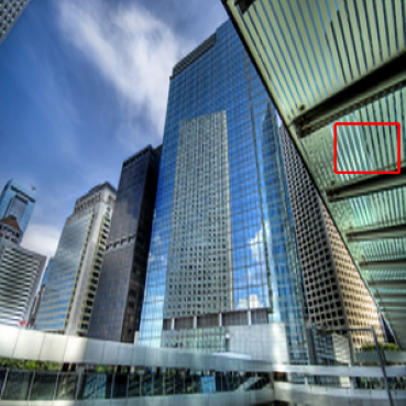
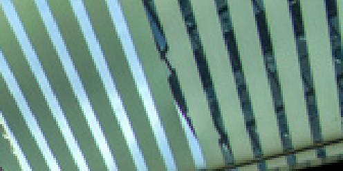
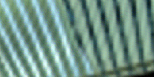
Urban100: img_061 ($\times$4) HR Bicubic $L_{1}$-norm [23] ASSL [48] SRP [49] ISS-P (ours)

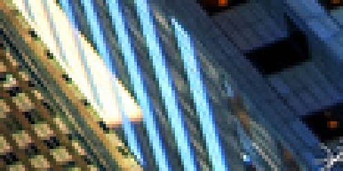
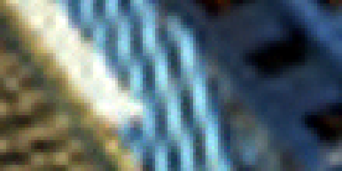
Urban100: img_012 ($\times$4) HR Bicubic $L_{1}$-norm [23] ASSL [48] SRP [49] ISS-P (ours)

Figure 3: Visualization comparison of different pruning methods on Urban100 [16] dataset. The pruning ratio is $0.99$.

Backbones	Methods	Set5		Set14		B100		Urban100		Manga109
		PSNR	SSIM	PSNR	SSIM	PSNR	SSIM	PSNR	SSIM	PSNR	SSIM
EDSR-L	scratch	29.60	0.8522	26.35	0.7312	25.92	0.7003	23.69	0.7303	27.28	0.8570
	$L_{1}$ norm [23]	29.61	0.8526	26.36	0.7318	25.93	0.7011	23.70	0.7313	27.35	0.8582
	ASSL [48]	29.85	0.8568	26.54	0.7368	26.07	0.7064	24.09	0.7461	27.93	0.8690
	SRP [49]	29.78	0.8558	26.47	0.7349	26.00	0.7036	23.89	0.7392	27.72	0.8656
	ISS-P (ours)	30.23	0.8628	26.74	0.7428	26.21	0.7109	24.43	0.7596	28.51	0.8783
CAT-R	scratch	32.19	0.8940	28.61	0.7816	27.58	0.7367	26.03	0.7846	30.50	0.8902
	$L_{1}$ norm [23]	32.19	0.8940	28.59	0.7814	27.58	0.7368	26.01	0.7842	30.52	0.9083
	ASSL [48]	32.08	0.8930	28.53	0.7803	27.54	0.7356	25.90	0.7809	30.35	0.9059
	SRP [49]	32.24	0.8950	28.61	0.7827	27.60	0.7382	26.09	0.7871	30.61	0.9096
	ISS-P (ours)	32.66	0.9008	28.93	0.7900	27.80	0.7444	26.94	0.8118	31.52	0.9197

Table 4: Performance comparison of different methods upon the representative CNN backbone, EDSR-L [26], and advanced transformer backbone, CAT-R [50], at the scale of the $\times 4$. The pruning ratio is $0.95$.

Methods	Scale	Set5		Set14		B100		Urban100		Manga109
		PSNR	SSIM	PSNR	SSIM	PSNR	SSIM	PSNR	SSIM	PSNR	SSIM
IHT	$\times$2	37.48	0.9585	33.01	0.9131	31.78	0.8947	30.56	0.9112	37.42	0.9738
ISS-R	$\times$2	37.38	0.9581	32.97	0.9121	31.72	0.8939	30.33	0.9082	37.16	0.9730
ISS-P	$\times$2	37.51	0.9587	33.05	0.9134	31.82	0.8952	30.68	0.9125	37.54	0.9741
IHT	$\times$3	37.04	0.9563	32.64	0.9091	31.49	0.8904	29.72	0.8998	36.47	0.9700
ISS-R	$\times$3	37.07	0.9566	32.66	0.9092	31.50	0.8906	29.70	0.8995	36.51	0.9704
ISS-P	$\times$3	37.31	0.9578	32.84	0.9112	31.66	0.8929	30.14	0.9059	37.00	0.9723
IHT	$\times$4	35.17	0.9448	31.49	0.8978	30.57	0.8781	27.95	0.8740	32.91	0.9519
ISS-R	$\times$4	35.37	0.9462	31.60	0.8983	30.66	0.8790	28.10	0.8730	33.31	0.9543
ISS-P	$\times$4	35.86	0.9496	31.89	0.9015	30.87	0.8819	28.40	0.8777	34.09	0.9584

Table 5: Ablation study of different methods over SwinIR under the pruning ratio of $0.9$ at different scales.

4 Experiment

Datasets and Backbones. Following the recent works [48, 49], we use DIV2K [38] and Flickr2K [26] as the training datasets. Five benchmark datasets are employed for the quantitative comparison and visualization, including Set5 [3], Set14 [46], B100 [28], Manga109 [29], and Urban100 [16]. We adopt PSNR and SSIM [43] as evaluation metrics by referring Y channels in the YCbCr space.

We train and evaluate the proposed method on representative backbones that cover convolutional network and transformer architectures: (1) SwinIR-Lightweight [25], which takes a sub-pixel convolutional layer [35] for the upsampling and a convolutional layer for the final reconstruction. (2) EDSR-L [26] that consists of $32$ residual blocks. (3) Cross-aggregation transformer [50] with regular rectangle window (CAT-R). We prune all of the learnable layers of the corresponding backbones from random initialization.

Implementation Details. We conduct the same augmentation procedure as previous works [48, 49] by implementing random rotation of $90^{\circ}$, $180^{\circ}$, $270^{\circ}$, and flipping horizontally. For network training, we adopt the image patches of $64\times 64$ with a batch size of 32. For computational efficiency, we set the batch size as $16$ for the ablation study. The training is performed upon an Adam [21] optimizer with $\beta_{1}$$=$$0.9$, $\beta_{2}$$=$$0.999$, and $\epsilon$$=$$10^{-8}$. The initial learning rate is $2\times e^{-4}$ with a half annealing upon every $2.5$$\times$$10^{5}$ iterations. We empirically determine the magnitude attenuation as $\alpha$$=$$0.95$. We set the total training iterations as $K$$=$$5$$\times$$10^{5}$ for benchmark comparison and $3\times 10^{5}$ for the ablation study. The pruning stage is $K_{\texttt{p}}$$=$$1$$\times$$10^{5}$. We implement the proposed method in PyTorch [32] on an NVIDIA RTX3090 GPU.

Compared Methods. We compare the proposed method with the classic baseline methods, i.e., training from scratch (dubbed as “Scratch”) and $L_{1}$-norm pruning [23] (denoted as “$L_{1}$-norm”), as well as the most recent pruning practices [48, 49] dedicated to SR models. All the methods are elaborated under the unstructured pruning, and we have no pre-trained dense networks at the beginning. For the fairness of the comparison, we facilitate the same backbone structure, training iterations, neural network initialization, and pruning ratios for different methods. Among them, ASSL [48] and SRP [49] are developed to remove the filters, but both are readily extendable to unstructured pruning. We keep the pruning constraints of both methods when operating on different backbones. For the proposed method, we use ISS-P as our final pruning treatment owing to its vigorous sparsity dynamics and promising performance.

4.1 Comparison with Advanced Pruning Methods

Performance Comparisons. We conduct a thorough quantitative comparison with different pruning ratios, i.e., $0.9$, $0.95$, and $0.99$, under the scale of $\times 2$, $\times 3$, and $\times$4. As shown in Table 1$\sim$3, the proposed ISS-P presents a promising performance by improving existing methods with a considerable margin. Notably, the advantage of the ISS-P is amplified when the scale or pruning ratio raises. Thanks to the dedicated design of ISS-P, a more regularized gradient flow is preserved, leading to better trainability, especially for sparse networks with larger scale or pruning ratios. We also provide more analysis on convergence in Section 4.2.

Visual Comparisons. We further visually compare the performance of the sparse networks trained with different pruning methods. In Fig. 3, we present the results at a challenging scale setting (i.e., $\times 4$) and very high pruning ratio (i.e., $0.99$). By comparison, the proposed ISS-P allows a more granular reconstruction, especially in textured areas with detailed visual ingredients, for example, the more clear contours of the buildings. Besides, the proposed method produces fewer distortions for regions with high gradients, e.g., by producing clearer and more consistent edges. These observations indicate a better modeling capacity, owing to an appropriate sparse architecture upon active sparse dynamics of ISS-P and a more promising optimization.

Different Backbones. In Table 4, we present the effectiveness of the proposed pruning method on different backbones. The ISS-P works favorably well by outperforming baseline and prevailing methods for SR, which is consistent with the results on SwinIR-Lightweight. Results on these backbones demonstrate that the proposed method is network structure-independent, which potentially eases the deployment of advanced SR networks and is actually an important property in practice.

4.2 ISS Analysis

Ablation Study. We perform ablation studies of the proposed method under the pruning ratio of $0.9$ at different scales. We specifically compare three ablated pruning methods, i.e., IHT, ISS-R, and ISS-P, which explore dynamic sparse structures with different weight annealing operators at each forward propagation procedure. The SwinIR-Lightweight [25] is adopted as the backbone. As shown in Table 5, the ISS-P consistently outperforms on different testing datasets. For example, the performance gap between ISS-P and ISS-R remains over $0.2$dB under the scale of $\times 4$. Note that ISS-R is inferior to the IHT at $\times 2$ scale but surpasses it at the $\times 4$. This suggests a strong resilience of ISS-R schedule in trainability preserving albeit a sub-optimal hyperparameter configuration in the growing regularization.

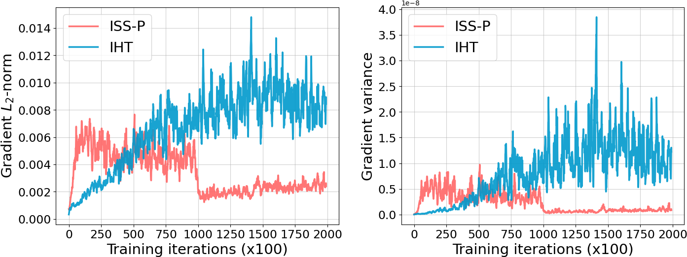
module.layers.0.residual_group.blocks.2.mlp.fc1 module.conv_after_body

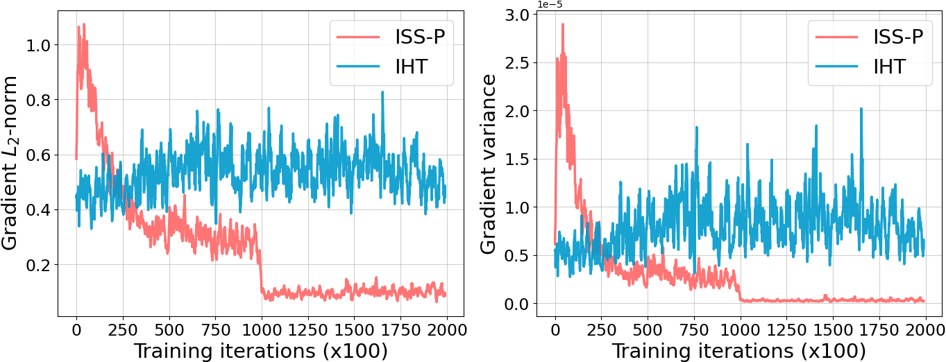
Figure 4: Trainability comparison of the IHT and ISS-P. The layer-wise gradient $L_{2}$-norm and variance in the pruning stage ($1$$\times$$10^{5}$ iterations) and the first $1$$\times$$10^{5}$ iterations of the fine-tuning stage are plotted. We choose two representative layers, i.e., a fully connected layer (top) and a convolution (bottom) from the SwinIR.

Trainability Analysis. Trainability depicts whether a network is easy to be optimized, which is highly associated to the sparse structures in the field of pruning. We find that ISS-P better preserves the trainability of the network. Intuitively, this is because the ISS-P better retains the network dynamical isometry [34] by better preserving the weight connections (dependencies) during the training, compared with IHT. We verify this point by observing the gradient $L_{2}$-norm and variance during the training. In Fig. 4, we find that the gradient norm of the ISS-P steadily converges in the pruning stage ($K_{\texttt{p}}<1\times 10^{5}$), so that the selected sparse network (taking effect at $K_{\texttt{p}}=1\times 10^{5}$) approaches the local minimum on the loss landscape at the end. Reversely, the gradient descent of IHT is still ongoing (i.e., iteration $k=2\times 10^{5}$), which indicates the network is harder to converge. A similar conclusion is also validated by comparing more regularized gradient variances of ISS-P against larger gradient variances of IHT. In addition, ISS-P allows better trainability throughout the network, regardless of the depth and layer types, as exampled by a shallow fully connected layer ($11$-th) and a deep convolutional layer ($101$-th).

5 Conclusion

In this work, we have studied the problem of efficient image super-resolution by the unstructured pruning treatment upon the network with randomly initialized weights. Specifically, we have proposed Iterative Soft Shrinkage-Percentage (ISS-P) method to iteratively shrink the weight with a small amount proportional to the magnitude, which has not only enabled a more dynamic sparse structure exploitation but also better retained the trainability of the network. The proposed method has been readily compatible with the off-the-shelf SR network designs, facilitating the sparse network acquisition and deployment.

References

- [1] Yue Bai, Huan Wang, Xu Ma, Yitian Zhang, Zhiqiang Tao, and Yun Fu. Parameter-efficient masking networks. In NeurIPS, 2022.
- [2] Yue Bai, Huan Wang, Zhiqiang Tao, Kunpeng Li, and Yun Fu. Dual lottery ticket hypothesis. In ICLR, 2022.
- [3] Marco Bevilacqua, Aline Roumy, Christine Guillemot, and Marie Line Alberi-Morel. Low-complexity single-image super-resolution based on nonnegative neighbor embedding. 2012.
- [4] Thomas Blumensath and Mike E Davies. Iterative hard thresholding for compressed sensing. Applied and computational harmonic analysis, 27(3):265–274, 2009.
- [5] Emmanuel J Candès, Justin Romberg, and Terence Tao. Robust uncertainty principles: Exact signal reconstruction from highly incomplete frequency information. IEEE Transactions on information theory, 52(2):489–509, 2006.
- [6] Emmanuel J Candes, Justin K Romberg, and Terence Tao. Stable signal recovery from incomplete and inaccurate measurements. Communications on Pure and Applied Mathematics, 59(8):1207–1223, 2006.
- [7] Chao Dong, Chen Change Loy, Kaiming He, and Xiaoou Tang. Learning a deep convolutional network for image super-resolution. In ECCV, 2014.
- [8] David L Donoho. Compressed sensing. IEEE Transactions on information theory, 52(4):1289–1306, 2006.
- [9] Alexey Dosovitskiy, Lucas Beyer, Alexander Kolesnikov, Dirk Weissenborn, Xiaohua Zhai, Thomas Unterthiner, Mostafa Dehghani, Matthias Minderer, Georg Heigold, Sylvain Gelly, et al. An image is worth 16x16 words: Transformers for image recognition at scale. In ICLR, 2021.
- [10] Song Han, Huizi Mao, and William J Dally. Deep compression: Compressing deep neural networks with pruning, trained quantization and huffman coding. In ICLR, 2016.
- [11] Song Han, Jeff Pool, John Tran, and William Dally. Learning both weights and connections for efficient neural network. In NeurIPS, 2015.
- [12] Kaiming He, Xiangyu Zhang, Shaoqing Ren, and Jian Sun. Deep residual learning for image recognition. In CVPR, 2016.
- [13] Yang He, Yuhang Ding, Ping Liu, Linchao Zhu, Hanwang Zhang, and Yi Yang. Learning filter pruning criteria for deep convolutional neural networks acceleration. In CVPR, 2020.
- [14] Yang He, Guoliang Kang, Xuanyi Dong, Yanwei Fu, and Yi Yang. Soft filter pruning for accelerating deep convolutional neural networks. In IJCAI, 2018.
- [15] Yihui He, Xiangyu Zhang, and Jian Sun. Channel pruning for accelerating very deep neural networks. In ICCV, 2017.
- [16] Jia-Bin Huang, Abhishek Singh, and Narendra Ahuja. Single image super-resolution from transformed self-exemplars. In CVPR, 2015.
- [17] Itay Hubara, Brian Chmiel, Moshe Island, Ron Banner, Joseph Naor, and Daniel Soudry. Accelerated sparse neural training: A provable and efficient method to find n: m transposable masks. In NeurIPS, 2021.
- [18] Justin Johnson, Alexandre Alahi, and Li Fei-Fei. Perceptual losses for real-time style transfer and super-resolution. In ECCV, 2016.
- [19] Jiwon Kim, Jung Kwon Lee, and Kyoung Mu Lee. Accurate image super-resolution using very deep convolutional networks. In CVPR, 2016.
- [20] Jiwon Kim, Jung Kwon Lee, and Kyoung Mu Lee. Deeply-recursive convolutional network for image super-resolution. In CVPR, 2016.
- [21] Diederik P Kingma and Jimmy Ba. Adam: A method for stochastic optimization. In ICLR, 2015.
- [22] Vadim Lebedev and Victor Lempitsky. Fast convnets using group-wise brain damage. In CVPR, 2016.
- [23] Hao Li, Asim Kadav, Igor Durdanovic, Hanan Samet, and Hans Peter Graf. Pruning filters for efficient convnets. In ICLR, 2017.
- [24] Yawei Li, Shuhang Gu, Christoph Mayer, Luc Van Gool, and Radu Timofte. Group sparsity: The hinge between filter pruning and decomposition for network compression. In CVPR, 2020.
- [25] Jingyun Liang, Jiezhang Cao, Guolei Sun, Kai Zhang, Luc Van Gool, and Radu Timofte. Swinir: Image restoration using swin transformer. In ICCV, 2021.
- [26] Bee Lim, Sanghyun Son, Heewon Kim, Seungjun Nah, and Kyoung Mu Lee. Enhanced deep residual networks for single image super-resolution. In CVPR workshop, 2017.
- [27] Mingbao Lin, Rongrong Ji, Yan Wang, Yichen Zhang, Baochang Zhang, Yonghong Tian, and Ling Shao. Hrank: Filter pruning using high-rank feature map. In CVPR, 2020.
- [28] David Martin, Charless Fowlkes, Doron Tal, and Jitendra Malik. A database of human segmented natural images and its application to evaluating segmentation algorithms and measuring ecological statistics. In ICCV, 2001.
- [29] Yusuke Matsui, Kota Ito, Yuji Aramaki, Azuma Fujimoto, Toru Ogawa, Toshihiko Yamasaki, and Kiyoharu Aizawa. Sketch-based manga retrieval using manga109 dataset. Multimedia Tools and Applications, 76:21811–21838, 2017.
- [30] Asit Mishra, Jorge Albericio Latorre, Jeff Pool, Darko Stosic, Dusan Stosic, Ganesh Venkatesh, Chong Yu, and Paulius Micikevicius. Accelerating sparse deep neural networks. arXiv preprint arXiv:2104.08378, 2021.
- [31] Junghun Oh, Heewon Kim, Seungjun Nah, Cheeun Hong, Jonghyun Choi, and Kyoung Mu Lee. Attentive fine-grained structured sparsity for image restoration. In CVPR, 2022.
- [32] Adam Paszke, Sam Gross, Francisco Massa, Adam Lerer, James Bradbury, Gregory Chanan, Trevor Killeen, Zeming Lin, Natalia Gimelshein, Luca Antiga, et al. Pytorch: An imperative style, high-performance deep learning library. In NeurIPS, 2019.
- [33] Russell Reed. Pruning algorithms-a survey. IEEE transactions on Neural Networks, 4(5):740–747, 1993.
- [34] Andrew M Saxe, James L McClelland, and Surya Ganguli. Exact solutions to the nonlinear dynamics of learning in deep linear neural networks. In ICLR, 2014.
- [35] Wenzhe Shi, Jose Caballero, Ferenc Huszár, Johannes Totz, Andrew P Aitken, Rob Bishop, Daniel Rueckert, and Zehan Wang. Real-time single image and video super-resolution using an efficient sub-pixel convolutional neural network. In CVPR, 2016.
- [36] Bin Sun, Yulun Zhang, Songyao Jiang, and Yun Fu. Hybrid pixel-unshuffled network for lightweight image super-resolution. In AAAI, 2023.
- [37] Vivienne Sze, Yu-Hsin Chen, Tien-Ju Yang, and Joel S Emer. Efficient processing of deep neural networks: A tutorial and survey. Proceedings of the IEEE, 105(12):2295–2329, 2017.
- [38] Radu Timofte, Eirikur Agustsson, Luc Van Gool, Ming-Hsuan Yang, and Lei Zhang. Ntire 2017 challenge on single image super-resolution: Methods and results. In CVPR workshop, 2017.
- [39] Ashish Vaswani, Noam Shazeer, Niki Parmar, Jakob Uszkoreit, Llion Jones, Aidan N Gomez, Łukasz Kaiser, and Illia Polosukhin. Attention is all you need. In NeurIPS, 2017.
- [40] Huan Wang and Yun Fu. Trainability preserving neural structured pruning. In ICLR, 2023.
- [41] Huan Wang, Can Qin, Yulun Zhang, and Yun Fu. Neural pruning via growing regularization. In ICLR, 2021.
- [42] Huan Wang, Yulun Zhang, Can Qin, Luc Van Gool, and Yun Fu. Global aligned structured sparsity learning for efficient image super-resolution. IEEE Transactions on Pattern Analysis and Machine Intelligence, 45(9):10974–10989, 2023.
- [43] Zhou Wang, Alan C Bovik, Hamid R Sheikh, and Eero P Simoncelli. Image quality assessment: from error visibility to structural similarity. IEEE transactions on image processing, 13(4):600–612, 2004.
- [44] Wei Wen, Chunpeng Wu, Yandan Wang, Yiran Chen, and Hai Li. Learning structured sparsity in deep neural networks. In NeurIPS, 2016.
- [45] Syed Waqas Zamir, Aditya Arora, Salman Khan, Munawar Hayat, Fahad Shahbaz Khan, and Ming-Hsuan Yang. Restormer: Efficient transformer for high-resolution image restoration. In CVPR, 2022.
- [46] Roman Zeyde, Michael Elad, and Matan Protter. On single image scale-up using sparse-representations. In Curves and Surfaces: 7th International Conference, Avignon, France, June 24-30, 2010, Revised Selected Papers 7, pages 711–730. Springer, 2012.
- [47] Yulun Zhang, Kunpeng Li, Kai Li, Lichen Wang, Bineng Zhong, and Yun Fu. Image super-resolution using very deep residual channel attention networks. In ECCV, 2018.
- [48] Yulun Zhang, Huan Wang, Can Qin, and Yun Fu. Aligned structured sparsity learning for efficient image super-resolution. In NeurIPS, 2021.
- [49] Yulun Zhang, Huan Wang, Can Qin, and Yun Fu. Learning efficient image super-resolution networks via structure-regularized pruning. In ICLR, 2022.
- [50] Chen Zheng, Yulun Zhang, Jinjin Gu, Yongbing Zhang, Linghe Kong, and Xin Yuan. Cross aggregation transformer for image restoration. In NeurIPS, 2022.