SUD²: Supervision by Denoising Diffusion Models for Image Reconstruction

Abstract

Many imaging inverse problems—such as image-dependent in-painting and dehazing—are challenging because their forward models are unknown or depend on unknown latent parameters. While one can solve such problems by training a neural network with vast quantities of paired training data, such paired training data is often unavailable. In this paper, we propose a generalized framework for training image reconstruction networks when paired training data is scarce. In particular, we demonstrate the ability of image denoising algorithms and, by extension, denoising diffusion models to supervise network training in the absence of paired training data.

1 Introduction

Imaging inverse problems can generally be described in terms of a forward operator $\mathcal{F}(\cdot)$ that maps a scene $x$ to a measurement $y$ according to

$$y=\mathcal{F}(x).$$ (1)

The goal of an image reconstruction algorithm is to recover $x$ from $y$.

Historically, computational imaging research has focused on solving inverse problems with known forward models. For instance, computed tomography’s forward model can be represented as a Radon transform, and magnetic resonance imaging’s forward model can be represented as 2D Fourier Transform. Knowledge of these forward models allows one to reconstruct scenes $x$ from measurements $y$ using any number of classical or learning-based algorithms [18].

Since the onset of the deep learning era, significant progress has been made in solving inverse problems which lack explicit forward models. By leveraging large amounts of training pairs $\{x_{i},y_{i}\}^{N}_{i=0}$, neural networks learn to directly map samples from a source distribution, $y_{i}$, to images from a target distribution, $x_{i}$. In doing so, the network implicitly learns the inverse operator $\mathcal{F}^{-1}$ without any explicit knowledge of the forward model $\mathcal{F}$.

The main drawback of deep learning methods is that their performance is directly related to the size and quality of the training dataset. As a result, these methods often struggle whenever little to no paired training data is available.

1.1 Problem setup

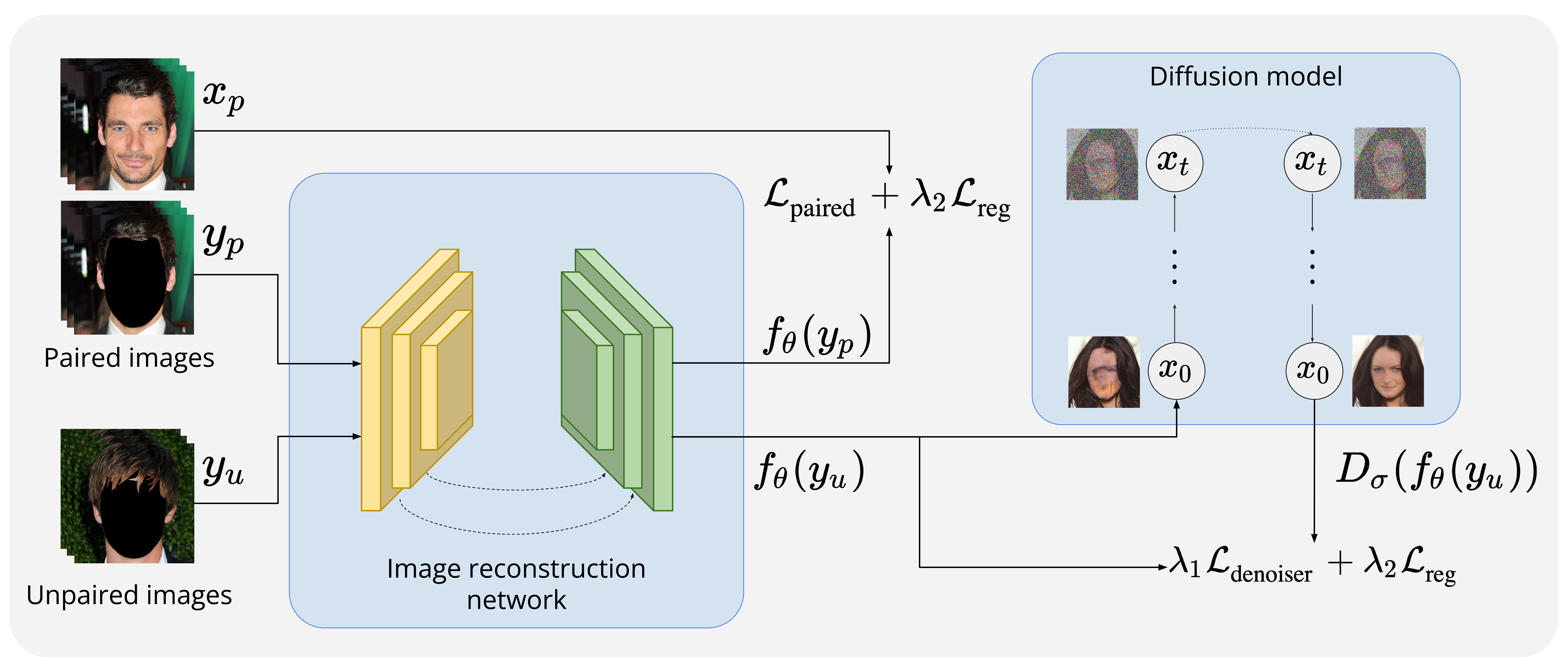
Our goal in this work is to train a network $f_{\theta}(\cdot)$ to reconstruct images/scenes $x$ from measurements $y$ using three sets of training data.

• A small set $P$ of paired examples $(x_{p},y_{p})$ drawn from the joint distribution $p_{x,y}$.

• A large set $U_{y}$ of unpaired measurements $y_{u}$ drawn from the marginal distribution $p_{y}$.

• A large set $U_{x}$ of unpaired images $x_{u}$ drawn from the marginal distribution $p_{x}$.

Such mixed datasets naturally occur in applications where gathering unpaired data is easy, but gathering paired data is a challenge. For instance, it is straightforward to capture images with fog and images without fog, but capturing two paired images of the same scene with and without fog (with all lighting conditions and other nuisance variations fixed) is very challenging. Often times, the latter paired dataset is restricted to only a few images captured in a lab.

A paired training set, $P$, allows one to optimize $f_{\theta}(\cdot)$ by minimizing the empirical risk

$$\mathcal{L}_{\text{paired}}=\frac{1}{|P|}\sum_{(x_{p},y_{p})\in P}\|x_{p}-f_{\theta}(y_{p})\|^{2},$$ (2)

where $|P|$ denotes the cardinality of $P$. However, as the size of $P$ decreases $\mathcal{L}_{\text{paired}}$ becomes a poor approximation of the true risk and $f_{\theta}(\cdot)$ overfits to the training set. As an alternative, we seek to leverage unpaired datasets $U_{x}$ and $U_{y}$ to improve the quality of our reconstructions.

1.2 Our contributions

In this work we introduce a novel semi-supervised learning framework for addressing image reconstruction problems, such as image dehazing, which lack an explicit forward model and for which gathering paired training data is challenging. Our central contributions are as follows;

• We generalize the supervision-by-denoising (SUD) semi-supervised learning technique from [28] to work on any image reconstruction task, not just medical image segmentation.

• We prove that SUD implicitly performs cross-entropy minimization and use this connection to identify its various failure modes.

• Based on our analysis, we identify three techniques to improve SUD: (1) sample correlation minimization, (2) noise injection, and (3) denoising diffusion models.

• We demonstrate that the resulting algorithm, which we call SUD², outperforms existing semi-supervised and unsupervised learning techniques, such as CycleGAN, on image in-painting and image dehazing.

2 Related work

2.1 Semi-supervised learning

While crowdsourcing platforms such as Amazon’s Mechanical Turk [23] can generate abundant labeled data for human-annotatable tasks like image segmentation, it’s all but impossible to hand-label training data for many imaging inverse problems. Given a foggy image, how would one generate corresponding clean image to use for training? Even in applications where hand-labeling is possible, it is often prohibitively expensive to perform at scale.

Semi-supervised learning (SSL) serves as a workaround for applying deep learning techniques in situations where paired data is scarce. Typically, SSL methods regularize network training by leveraging information extracted from unpaired data and generally fall into two distinct categories; pseudo-labelling methods and consistency regularization methods [27]. Pseudo-labelling methods [13] help supervise training by generating fake labels on unpaired data samples, which allows the training of networks in a fully-supervised manner. In contrast, consistency regularization methods like temporal ensembling [11] and mean teacher models [24] enforce a regularization objective during training that makes the network more robust to perturbations in the data.

Our method borrows ideas from both categories of SSL methods. Similar to pseudo-labelling methods, we generate fake labels on unpaired data by incorporating a denoising diffusion probabilistic model (DDPM) [9] into the training pipeline. Additionally, following consistency regularization methods, we impose a regularization objective that encourages our image reconstruction network to produces diverse outputs.

2.2 Regularization-by-denoising

Image denoising algorithms (denoisers) can serve as powerful priors on the form and distribution of natural images [7, 25, 14]. Regularization-by-denoising (RED) [21, 19] is a regularization technique that leverages an image denoiser to solve classical single-image imaging inverse problems. Given an known forward model $\mathcal{F}$ and a single measurement $y$, RED (under a white Gaussian prior on the measurement noise) tries to reconstruct the unknown scene $x$ by minimizing

$$\arg\min_{x}\|y-\mathcal{F}(x)\|^{2}+\rho(x),$$ (3)

where

$$\rho(x)=\frac{1}{2}x^{T}\left[x-D(x)\right],$$ (4)

and $D(\cdot)$ represents a denoiser like BM3D [5] or DnCNN [30]. Variations on this idea have recently been combined with diffusion models as well [4].

One simplified interpretation of the RED regularization objective (4) is that a good denoiser $D(\cdot)$ will project $x$ onto the manifold $\mathcal{M}$ of natural images. If $x$ is far from that manifold $\rho(x)$ will be large, whereas if $x$ is already close to this manifold, $D(x)$ will change it very little and $\rho(x)$ will be small.

Similar to RED, our method leverages an image denoiser. However, instead of using the denoiser to regularize classical inverse imaging optimization objectives, we follow [28] and use an image denoiser to regularize the training of deep neural networks. That is, we are using denoiser to regularize a function rather than an image. The resulting function/reconstruction network, unlike the RED, is non-iterative and does not require explicit knowledge of the forward model $\mathcal{F}$.

Figure 1: Overview of the training pipeline. Block diagram of the semi-supervised training pipeline used in our experiments. The pre-trained diffusion model supervises training by pushing outputs of the image reconstruction network towards the desired target image distribution. Note that only the image reconstruction network (a standard U-net in our experiments) is used at inference time.

3 Methods

3.1 Supervision-by-denoising

Young et al. [28] recently introduced the supervision-by-denoising (SUD) framework which takes the ideas behind regularization-by-denoising [21] and extends them to enable semi-supervised learning. The intuition behind SUD is that a pretrained image denoiser, $D_{\sigma}(u)$, (which can be trained using the set $U_{x}$ of unpaired images) encodes strong priors on the distribution $p_{x}$. SUD enforces that the network’s reconstructions $f_{\theta}(y_{u})$ on the unpaired training data are “consistent” with the priors encoded in the denoiser.

When used in combination with an $\ell_{2}$ loss and without temporal-ensembling/damping, SUD effectively minimizes

$$\mathcal{L}_{\text{paired}}+\lambda_{1}\mathcal{L}_{\text{denoiser}},$$ (5)

where $\lambda_{1}$ is a tuning parameter and

$$\mathcal{L}_{\text{denoiser}}=\frac{1}{|U_{y}|}\sum_{y_{u}\in U_{y}}\|f_{\theta}(y_{u})-z_{u}\|^{2},$$ (6)

where $z_{u}=D_{\sigma}(f_{\theta}(y_{u}))$. When updating the network weights $\theta$ to minimize (6), SUD treats $z_{u}$ as a fixed pseudo-label and does not propagate gradients through the denoiser. That is, SUD defines the gradient of $\mathcal{L}_{\text{denoiser}}$ with respect to a single reconstruction $f_{\theta}(y_{u})$ as

$$\nabla_{f_{\theta}(y_{u})}\mathcal{L}_{\text{denoiser}}=\frac{2[f_{\theta}(y_{u})-D_{\sigma}(f_{\theta}(y_{u}))]}{|U_{y}|}.$$ (7)

As demonstrated in [28], SUD is a powerful and effective semi-supervised learning technique in the context of medical segmentation, where the goal is to map an image to a discrete-valued segmentation map. Using only a handful paired images and segmentation maps, Young et al. were able to train a denoiser to segment brains, kidneys, and tumors.

Unfortunately, we found that without modification, SUD, with or without temporal ensembling, was far less effective at general image restoration tasks. As illustrated in Figure 2, minimizing the SUD loss for CelebA face inpainting leads to mode collapse.

3.2 Understanding SUD

In this section we analyze SUD in order to identify and overcome its weaknesses.

Theorem 3.1.

When $D_{\sigma}$ is a minimum-mean-squared error (MMSE) Gaussian denoiser, minimizing $\mathcal{L}_{\text{denoiser}}$ minimizes the cross entropy between the distribution of $f_{\theta}(y_{u})$ and the smoothed version of $p_{x}$.

Proof.

Let $\nu$ follow an independent zero-mean white Gaussian distribution with variance $\sigma^{2}$. We will use $\nu$ to smooth the distributions $p_{x}$ (recall $p_{x+\nu}=p_{x}*p_{\nu}$, where $*$ denotes convolution) so that we can take advantage of Tweedie’s Formula, as described below.

The cross entropy between $p_{f_{\theta}(y)}$ and $p_{x+\nu}$ is, by definition,

$$H(p_{f_{\theta}(y)},p_{x+\nu}) =-\mathbb{E}_{f_{\theta}(y)}[\ln p_{x+\nu}(f_{\theta}(y))].$$ (8)

We can form a Monte-Carlo approximate of the expectation in (8) by averaging over $U_{y}$:

$$H(p_{f_{\theta}(y)},p_{x+\nu})\approx-\frac{1}{|U_{y}|}\sum_{y_{u}\in U_{y}}\ln p_{x+\nu}(f_{\theta}(y_{u})).$$ (9)

Then, we can express the gradient of this loss with respect to a reconstruction $f_{\theta}(y_{u})$ as

$$\nabla_{f_{\theta}(y_{u})}H(p_{f_{\theta}(y)},p_{x+\nu})$$

$$\approx-\frac{\nabla_{f_{\theta}(y_{u})}\ln p_{x+\nu}(f_{\theta}(y_{u}))}{|U_{y}|}.$$ (10)

To efficiently evaluate (3.2) we turn to Tweedie’s Formula. Tweedie’s Formula [6] states that for a signal corrupted with zero-mean additive white Gaussian noise, $r=x+\nu$ where $\nu\sim\mathcal{N}(0,\sigma^{2}\mathbf{I})$, the output of a MMSE denoiser $D_{\sigma}(\cdot)$ (and by extension a neural network trained to act as a MMSE denoiser) can be expressed as

$$D_{\sigma}(r)=r+\sigma^{2}\nabla_{r}\ln p_{x+\nu}(r).$$ (11)

In other words, denoisers perform gradient ascent on the log-likelihood of $p_{x+\nu}$ where the step size corresponds to the noise variance. Accordingly, we can express the gradient of the log-likelihood in terms of the denoiser’s residual:

$$\nabla_{r}\ln p_{x+\nu}(r)=\frac{D_{\sigma}(r)-r}{\sigma^{2}}.$$ (12)

By applying Tweedie’s formula to (3.2) we arrive at

$$\nabla_{f_{\theta}(y_{u})}H(p_{f_{\theta}(y)},p_{x+\nu})\approx\frac{[f_{\theta}(y_{u})-D_{\sigma}(f_{\theta}(y_{u}))]}{\sigma^{2}|U_{y}|}.$$ (13)

Up to constants, this is the same expression as the SUD gradients defined in (7). As such, the SUD denoiser loss minimizes the cross entropy between $p_{f_{\theta}(y)}$ and $p_{x+\nu}$. ∎

w/ $\mathcal{L}_{\text{reg}}$	\begin{overpic}[width=39.0242pt]{img/mode_collapse/epoch10_1.png}\end{overpic}	\begin{overpic}[width=39.0242pt]{img/mode_collapse/epoch20_1.png}\end{overpic}	\begin{overpic}[width=39.0242pt]{img/mode_collapse/epoch30_1.png}\end{overpic}	\begin{overpic}[width=39.0242pt]{img/mode_collapse/epoch40_1.png}\end{overpic}	\begin{overpic}[width=39.0242pt]{img/mode_collapse/epoch50_1.png}\end{overpic}
	Epoch 10	Epoch 20	Epoch 30	Epoch 40	Epoch 50

Figure 2: SUD with and without correlation minimization. Without a correlation loss to regularize reconstructions, the SUD denoising objective causes network outputs to converge to a mode—in this case a washed out image.

Corollary 3.2.

Minimizing $\mathcal{L}_{\text{denoiser}}$ encourages mode collapse.

Proof.

Minimizing $\mathcal{L}_{\text{denoiser}}$ minimizes the cross entropy between $p_{f_{\theta}(y_{u})}$ and $p_{x+\nu}$. The cross entropy of $H(p,q)$ of two distributions $p$ and $q$ is minimized with respect to $p$ when $p$ is a dirac distribution with a non-zero support where distribution $q$ is largest, i.e., a mode. ∎

Examples of SUD leading to mode collapse are presented in Figure 2.

Corollary 3.3.

Minimizing $\mathcal{L}_{\text{denoiser}}$ can encourage blurry reconstructions.

Proof.

Minimizing $\mathcal{L}_{\text{denoiser}}$ minimizes the cross entropy between $p_{f_{\theta}(y_{u})}$ and $p_{x+\nu}$ and will result in solutions $f_{\theta}(y_{u})$ that maximize $p_{x+\nu}(f_{\theta}(y_{u}))$. For sufficiently large $\sigma$, $p_{x+\nu}$ is maximized not where $p_{x}$ is large (along the manifold of natural images) but rather at some point in between high-probability points. ∎

A toy example illustrating how introducing noise onto a random variable can move its distribution’s maxima is presented in Figure 3.

\begin{overpic}[width=71.54768pt]{img/Toy/Dist1.png}\end{overpic}	\begin{overpic}[width=71.54768pt]{img/Toy/Dist2.png}\end{overpic}	\begin{overpic}[width=71.54768pt]{img/Toy/Dist3.png}\end{overpic}
$p_{x}$	$p_{x+\nu_{1}}$	$p_{x+\nu_{2}}$

Figure 3: PDFs of a bimodal distribution with varying amounts of noise. Adding sufficient noise can move the distribution’s mode.

3.3 Improving SUD

To fight mode collapse, we introduce an additional penalty, $\mathcal{L}_{\text{reg}}$ into the SUD loss which encourages diverse outputs. That is, we minimize

$$\mathcal{L}_{\text{paired}}+\lambda_{1}\mathcal{L}_{\text{denoiser}}+\lambda_{2}\mathcal{L}_{\text{reg}}$$ (14)

where $\lambda_{1}$ and $\lambda_{2}$ are scalar weights on each loss term.

Theorem 3.4.

When no paired training data is present, SUD with $\lambda_{1}=\frac{1}{2\sigma^{2}}$, $\lambda_{2}=1$, and $\mathcal{L}_{\text{reg}}=-H(p_{f_{\theta}(y)})$ minimizes the KL divergence between the distributions of $f_{\theta}(y)$ and $x+\nu$.

Proof.

Our results from Theorem 3.1 indicate $\frac{1}{2\sigma^{2}}\mathcal{L}_{\text{denoiser}}$ and $H(p_{f_{\theta}(y)},p_{x+\nu})$ have the same gradients. Thus minimizing

$$\frac{1}{2\sigma^{2}}\mathcal{L}_{\text{denoiser}}+\mathcal{L}_{\text{reg}}$$ (15)

minimizes

$$H(p_{f_{\theta}(y)},p_{x+\nu})-H(p_{f_{\theta}(y)}).$$ (16)

The latter expression is the definition of KL-divergence between the distributions of $f_{\theta}(y)$ and $x+\nu$. ∎

3.3.1 Correlation minimization

Computing and maximizing the entropy $H(p_{f_{\theta}(y_{u})})$ is computationally intractable. To get around this hurdle, we instead encourage sample diversity as follows: (1) we use a U-net architecture as our reconstruction network $f_{\theta}(\cdot)$, (2) we let $a_{u}$ represent the intermediate activation of $f_{\theta}$ to inputs $y_{u}$, and (3) we then penalize correlations between activations.

Specifically, in each mini-batch, we compute the normalized covariance matrix on the intermediate outputs from the encoder block of our network. Diagonal entries of the matrix—which contain the correlation coefficient of each vector with itself—are all equal to 1 by definition. Non-diagonal entries of the matrix contain the Pearson correlation coefficient (PCC) between the latent vectors in a mini-batch.

PCC identifies linear correlations between the latent vectors, where a value of 0 signifies linearly uncorrelated samples, a value 1 signifies a positive linear correlation between samples, and a value of $-1$ signifies a negative linear correlation between samples. By minimizing this value for each entry in the correlation matrix, we encourage network to produce outputs which are uncorrelated in latent space.

3.3.2 Noise injection

with noise	\begin{overpic}[width=62.87344pt]{img/noise_ablation/noise_1.png}\end{overpic}	\begin{overpic}[width=62.87344pt]{img/noise_ablation/noise_3.png}\end{overpic}	\begin{overpic}[width=62.87344pt]{img/noise_ablation/noise_4.png}\end{overpic}
without noise	\begin{overpic}[width=62.87344pt]{img/noise_ablation/no_noise_1.png}\end{overpic}	\begin{overpic}[width=62.87344pt]{img/noise_ablation/no_noise_3.png}\end{overpic}	\begin{overpic}[width=62.87344pt]{img/noise_ablation/no_noise_4.png}\end{overpic}

Figure 4: SUD with and without noise injection. Injecting noise onto the reconstructed images before denoising them results in more realistic-looking reconstructions.

SUD compares the distribution of the reconstructions $f_{\theta}(y)$ with the distribution $p_{x+\nu}$. As noted in the previous section, this encourages solutions for which $p_{x+\nu}$ is large but $p_{x}$ is small: i.e., it can produce solutions off of the manifold of natural images.

To alleviate this problem, we inject noise onto the reconstructions $f_{\theta}(y_{u})$ before passing them through the denoiser. That is, we redefine $\nabla_{f_{\theta}(y_{u})}\mathcal{L}_{\text{denoiser}}$ as

$$\nabla_{f_{\theta}(y_{u})}\mathcal{L}_{\text{denoiser}}=\frac{2[f_{\theta}(y_{u})-D_{\sigma}(f_{\theta}(y_{u})+\nu_{2})]}{|U_{y}|},$$ (17)

where $\nu_{2}\sim N(0,\sigma_{2}^{2}\mathbf{I})$.

This simple modification allows us to compare the smoothed distribution $p_{f_{\theta}(y)+\nu_{2}}$ with the smoothed distribution $p_{x+\nu}$. As demonstrated in Figure 4, noise injection produces reconstructions of considerably higher quality.

3.3.3 Diffusion models

DDPM	\begin{overpic}[width=62.87344pt]{img/diffusion_ablation/diffusion_1.png}\end{overpic}	\begin{overpic}[width=62.87344pt]{img/diffusion_ablation/diffusion_2.png}\end{overpic}	\begin{overpic}[width=62.87344pt]{img/diffusion_ablation/diffusion_3.png}\end{overpic}
AE	\begin{overpic}[width=62.87344pt]{img/diffusion_ablation/denoiser_1.png}\end{overpic}	\begin{overpic}[width=62.87344pt]{img/diffusion_ablation/denoiser_2.png}\end{overpic}	\begin{overpic}[width=62.87344pt]{img/diffusion_ablation/denoiser_3.png}\end{overpic}

Figure 5: SUD with and without denoising diffusion models. Image in-painting samples generated by SUD with a multi-step denoising diffusion model (top) and a one-step autoencoder image denoiser (bottom). SUD training with the denoising diffusion model produces higher-quality reconstructions.

As mentioned in Section 2.2, an alternative and more heuristic interpretation of denoising algorithms is that they are projecting the reconstructions onto a manifold $\mathcal{M}$ of allowable reconstructions, e.g., faces or “natural images”. Traditional denoising algorithms perform this projection in a single step. However, existing theory [26] suggests that one should navigate image manifolds gradually, in a smooth-to-rough/coarse-to-fine manner.

Loosely inspired by this observation, we propose replacing our single-step MMSE denoising algorithm with a multi-step denoising diffusion probabilistic model (DDPMs) [9]. That is, we replace our denoiser $D_{\sigma}(\cdot)$ used in (17) with an iterative forward “noising” operator $F(\cdot)$ and an iterative reverse “denoising” operator $R(\cdot)$ such that $D_{\sigma}(f_{\theta}(y_{u})+\nu)=R(F(f_{\theta}(y_{u})))$. The definitions for each operator are expressed as

(18)

where $\alpha$ controls the noise variance at each time step $t$, $z\sim\mathcal{N}(0,I)$, $\epsilon$ represents a diffusion network with weights $\tau$, and $\bar{\alpha}_{t}=\prod^{t}_{i}\alpha_{i}$.

Conceptually, the DDPM serves to first project $r$ onto the smooth manifold of noisy images and then gradually project $r$ onto correspondingly less smooth manifolds of less noisy images. As demonstrated in Figure 5, training with a DDPM produces higher quality results than training with a denoising auto-encoder.

3.4 SUD²

We refer to SUD, including all the aforementioned modifications, as SUD². Ablation studies characterizing the relative importance of correlation minimization, noise injection, and denoising diffusion models are provided in the supplement.

4 Experiments

In the following experiments, we evaluate our method both quantitatively and qualitatively against baselines. All methods below are trained on 5 paired images, and the semi-supervised methods are trained on additional unpaired images.

The backbone architecture for our image reconstruction network is a U-net [22] consisting of 4 down-sampling and up-sampling blocks—implemented using strided convolutions—with skip connections between them. Each down/up-sampling block contains two convolutional layers, each with batch normalization and a Leaky ReLU activation function [15]. The denoising diffusion models used in our experiments have a similar U-net architecture, albeit with 6 down/up-sampling blocks and spatial self-attention. Similarly, our denoising networks use an autoencoder backbone identical to the image reconstruction U-net, but with skip connections removed.

We train all of the image reconstruction networks on $4\times$ Nvidia RTX A5000 GPUs using an Adam optimizer with an initial learning rate of $1\times 10^{-3}$, a weight decay of $1\times 10^{-4}$, and a batch size of 8 for 50 epochs. Additionally, we resize images to $256\times 256$ resolution and normalize pixel intensities between $[-1,1]$ before training.

When evaluating our method on the experiments below, we set $\lambda_{1}=0.01,\lambda_{2}=10$ and supervise training by walking 400 steps along the forward diffusion process before walking 400 steps along the reverse diffusion process. Generally, we find $[300,700]$ steps to be a reasonable range to take. Traversing more than 700 steps along the diffusion chain adds excess amounts of noise to the image, resulting in an image which no longer resembles the input image. In contrast, traversal of less than 300 steps yields images which are approximately identical to the input images—making them poor targets for supervision.

Instead of explicitly setting the gradient of the loss, we equivalently implement (17) by disabling backpropagation of gradients through the diffusion model $D_{\sigma}(\cdot)$ before computing the $\ell_{2}$ loss between $f_{\theta}(y_{u})$ and $D_{\sigma}(f_{\theta}(y_{u}))$. We also add a perceptual loss—specifically Learned Perceptual Image Patch Similarity (LPIPS) [31]—to $\mathcal{L}_{\text{paired}}$ and $\mathcal{L}_{\text{denoiser}}$ as we empirically find it to help produce better quality reconstructions.

4.1 Image in-painting

\begin{overpic}[width=62.87344pt]{img/teaser/celeba_sup_1.png}\end{overpic}

\begin{overpic}[width=62.87344pt]{img/teaser/celeba_cyclegan_1.png}\end{overpic}

\begin{overpic}[width=62.87344pt]{img/teaser/celeba_labels_1.png}\end{overpic}

\begin{overpic}[width=62.87344pt]{img/teaser/celeba_sud_1.png}\end{overpic}

\begin{overpic}[width=62.87344pt]{img/teaser/celeba_sud2_1.png}\end{overpic}

\begin{overpic}[width=62.87344pt]{img/teaser/celeba_sup_2.png}\end{overpic}

\begin{overpic}[width=62.87344pt]{img/teaser/celeba_cyclegan_2.png}\end{overpic}

\begin{overpic}[width=62.87344pt]{img/teaser/celeba_labels_2.png}\end{overpic}

\begin{overpic}[width=62.87344pt]{img/teaser/celeba_sud_2.png}\end{overpic}

\begin{overpic}[width=62.87344pt]{img/teaser/celeba_sud2_2.png}\end{overpic}

(a) Input

\begin{overpic}[width=62.87344pt]{img/teaser/celeba_sup_3.png}\end{overpic}

(b) Supervised

\begin{overpic}[width=62.87344pt]{img/teaser/celeba_cyclegan_3.png}\end{overpic}

(c) CycleGAN

\begin{overpic}[width=62.87344pt]{img/teaser/celeba_labels_3.png}\end{overpic}

(d) CycleGAN-SSL

\begin{overpic}[width=62.87344pt]{img/teaser/celeba_sud_3.png}\end{overpic}

(e) SUD

\begin{overpic}[width=62.87344pt]{img/teaser/celeba_sud2_3.png}\end{overpic}

(f) $\text{SUD}^{2}$

(g) Reference

Figure 6: Qualitative in-painting results. The images above show inference results from several methods on CelebAMask-HQ in-painting. All methods are trained on 5 pairs of masks and faces. Semi-supervised methods (CycleGAN-SSL, SUD, SUD²) are trained on an additional 1000+12,500 unpaired faces.

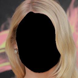
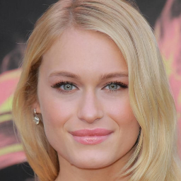
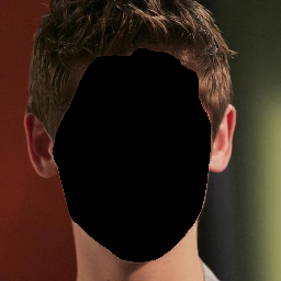
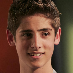
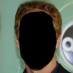
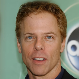
Image in-painting is a generative process for reconstructing missing regions of an image such that restored image fits a desired—often natural—image distribution. We test our method on the CelebAMask-HQ dataset [12], which contains 30,000 images of $512\times 512$ resolution and their corresponding segmentation maps. This dataset allows us to learn a strong prior since the image distribution is relatively constrained—all images are one-quarter head shots of celebrities.

In this experiment, we mask out the subject’s face from each image and train a few shot, semi-supervised in-painting network on 5 paired images and 1000+12,500 unpaired images. The 12,500 unpaired images are used to pre-train a blind Gaussian denoiser, a diffusion model, and a CycleGAN [33]. Note that the denoiser and diffusion model are only trained on 12,500 faces without a mask applied. However, we train the CycleGAN on non-corresponding pairs of 12,500 faces without a mask applied and 12,500 faces with a mask applied to give it the best possible performance. As an additional baseline, we also train an image reconstruction network using the pre-trained CycleGAN as a pseudo-label generator, which we refer to as CycleGAN-SSL.

Despite requiring far fewer images than both CycleGAN baselines, SUD² produces faces which most closely resemble the ground truth distribution. Furthermore, the strong prior imposed by the pre-trained diffusion model results in reconstructions with more defined facial structure compared to baseline methods. Notably, as described in Corollary (3.2), the SUD baseline collapses to a mode during training with high probability, yielding highly correlated reconstructions.

Quantitatively, SUD² achieves the most consistent results across our test set of $768$ images, with a $48\%$ higher average PSNR over CycleGAN-SSL and a $43\%$ lower average FID score compared to the supervised baseline. Although CycleGAN achieves the best FID score overall, it tends to produce qualitatively poor faces with disproportionately sized features, which is reflected in its poor PSNR, SSIM, and LPIPS scores. Likewise, while the supervised baseline achieves PSNR, SSIM, and LPIPS scores comparable to SUD², it often generates faces with missing features (i.e. eyes, nose, mouth), which is indicated by its high FID score.

Image in-painting
Method	PSNR$\uparrow$	SSIM$\uparrow$	LPIPS$\downarrow$	FID$\downarrow$
Supervised	18.44	0.71	0.29	0.48
CycleGAN	8.77	0.23	0.66	0.17
CycleGAN-SSL	11.38	0.60	0.39	1.14
SUD	11.28	0.29	0.69	3.07
$\text{SUD}^{2}$ (Ours)	18.71	0.71	0.28	0.31

Figure 7: Quantitative image in-painting results. This table lists the average scores attained by each method on the CelebAMask-HQ image in-painting test set. The best scores are bolded for readability.

Image dehazing
Method	PSNR$\uparrow$	SSIM$\uparrow$	LPIPS$\downarrow$
Supervised	17.65	0.66	0.44
CycleGAN	12.80	0.22	0.64
$\text{SUD}^{2}$ (Ours)	17.74	0.64	0.37

Figure 8: Quantitative image dehazing results. This table lists the median scores attained by each method on the REVIDE image dehazing test set. The best scores are bolded for readability.

\begin{overpic}[width=86.72267pt]{img/haze/supervise_1.png} \put(5.0,5.0){\scriptsize{\color[rgb]{1,1,1}\definecolor[named]{pgfstrokecolor}{rgb}{1,1,1}\pgfsys@color@gray@stroke{1}\pgfsys@color@gray@fill{1}{PSNR:16.53}}} \put(55.0,5.0){\scriptsize{\color[rgb]{1,1,1}\definecolor[named]{pgfstrokecolor}{rgb}{1,1,1}\pgfsys@color@gray@stroke{1}\pgfsys@color@gray@fill{1}{SSIM:0.58}}} \end{overpic}

\begin{overpic}[width=86.72267pt]{img/haze/cyclegan_1.png} \put(5.0,5.0){\scriptsize{\color[rgb]{1,1,1}\definecolor[named]{pgfstrokecolor}{rgb}{1,1,1}\pgfsys@color@gray@stroke{1}\pgfsys@color@gray@fill{1}{PSNR:15.68}}} \put(55.0,5.0){\scriptsize{\color[rgb]{1,1,1}\definecolor[named]{pgfstrokecolor}{rgb}{1,1,1}\pgfsys@color@gray@stroke{1}\pgfsys@color@gray@fill{1}{SSIM:0.42}}} \end{overpic}

\begin{overpic}[width=86.72267pt]{img/haze/sud2_1.png} \put(5.0,5.0){\scriptsize{\color[rgb]{1,1,1}\definecolor[named]{pgfstrokecolor}{rgb}{1,1,1}\pgfsys@color@gray@stroke{1}\pgfsys@color@gray@fill{1}{PSNR:17.76}}} \put(55.0,5.0){\scriptsize{\color[rgb]{1,1,1}\definecolor[named]{pgfstrokecolor}{rgb}{1,1,1}\pgfsys@color@gray@stroke{1}\pgfsys@color@gray@fill{1}{SSIM:0.66}}} \end{overpic}

\begin{overpic}[width=86.72267pt]{img/haze/haze_sup_1.png} \put(5.0,5.0){\scriptsize{\color[rgb]{1,1,1}\definecolor[named]{pgfstrokecolor}{rgb}{1,1,1}\pgfsys@color@gray@stroke{1}\pgfsys@color@gray@fill{1}{PSNR:21.70}}} \put(55.0,5.0){\scriptsize{\color[rgb]{1,1,1}\definecolor[named]{pgfstrokecolor}{rgb}{1,1,1}\pgfsys@color@gray@stroke{1}\pgfsys@color@gray@fill{1}{SSIM:0.75}}} \end{overpic}

\begin{overpic}[width=86.72267pt]{img/haze/haze_cyclegan_1.png} \put(5.0,5.0){\scriptsize{\color[rgb]{1,1,1}\definecolor[named]{pgfstrokecolor}{rgb}{1,1,1}\pgfsys@color@gray@stroke{1}\pgfsys@color@gray@fill{1}{PSNR:19.66}}} \put(55.0,5.0){\scriptsize{\color[rgb]{1,1,1}\definecolor[named]{pgfstrokecolor}{rgb}{1,1,1}\pgfsys@color@gray@stroke{1}\pgfsys@color@gray@fill{1}{SSIM:0.70}}} \end{overpic}

\begin{overpic}[width=86.72267pt]{img/haze/haze_sud2_1.png} \put(5.0,5.0){\scriptsize{\color[rgb]{1,1,1}\definecolor[named]{pgfstrokecolor}{rgb}{1,1,1}\pgfsys@color@gray@stroke{1}\pgfsys@color@gray@fill{1}{PSNR:22.01}}} \put(55.0,5.0){\scriptsize{\color[rgb]{1,1,1}\definecolor[named]{pgfstrokecolor}{rgb}{1,1,1}\pgfsys@color@gray@stroke{1}\pgfsys@color@gray@fill{1}{SSIM:0.76}}} \end{overpic}

(a) Input

\begin{overpic}[width=86.72267pt]{img/haze/haze_sup_2.png} \put(5.0,5.0){\scriptsize{\color[rgb]{1,1,1}\definecolor[named]{pgfstrokecolor}{rgb}{1,1,1}\pgfsys@color@gray@stroke{1}\pgfsys@color@gray@fill{1}{PSNR:16.00}}} \put(55.0,5.0){\scriptsize{\color[rgb]{1,1,1}\definecolor[named]{pgfstrokecolor}{rgb}{1,1,1}\pgfsys@color@gray@stroke{1}\pgfsys@color@gray@fill{1}{SSIM:0.54}}} \end{overpic}

(b) Supervised

\begin{overpic}[width=86.72267pt]{img/haze/haze_cyclegan_2.png} \put(5.0,5.0){\scriptsize{\color[rgb]{1,1,1}\definecolor[named]{pgfstrokecolor}{rgb}{1,1,1}\pgfsys@color@gray@stroke{1}\pgfsys@color@gray@fill{1}{PSNR: 13.09}}} \put(55.0,5.0){\scriptsize{\color[rgb]{1,1,1}\definecolor[named]{pgfstrokecolor}{rgb}{1,1,1}\pgfsys@color@gray@stroke{1}\pgfsys@color@gray@fill{1}{SSIM:0.35}}} \end{overpic}

(c) CycleGAN

\begin{overpic}[width=86.72267pt]{img/haze/haze_sud2_2.png} \put(5.0,5.0){\scriptsize{\color[rgb]{1,1,1}\definecolor[named]{pgfstrokecolor}{rgb}{1,1,1}\pgfsys@color@gray@stroke{1}\pgfsys@color@gray@fill{1}{PSNR:14.14}}} \put(55.0,5.0){\scriptsize{\color[rgb]{1,1,1}\definecolor[named]{pgfstrokecolor}{rgb}{1,1,1}\pgfsys@color@gray@stroke{1}\pgfsys@color@gray@fill{1}{SSIM:0.62}}} \end{overpic}

(d) $\text{SUD}^{2}$

(e) Reference

Figure 9: Dehazing results. Inference results comparing our method against baselines on dehazing REVIDE bedrooms. All methods use the same network architecture (U-net). All methods are provided 5 hazy / clear image pairs, 200 unpaired hazy images.

4.2 Dehazing

4.2.1 Haze forward model

Image dehazing is a challenging imaging inverse problem, where the objective is to remove degradations caused by small particulates in the air which obstruct visibility. Typically, dehazing methods approximate the hazy image formation as an depth-dependent attenuation process, defined by the well-known dichromatic atmospheric scattering model [16, 17]

$$I(x,y)=J(x,y)t(x,y)+A(1-t(x,y)).$$ (19)

Each pixel in the hazy image $I$ is obtained by attenuating pixels in the clear image $J$ according to a transmission map $t$ dependent on depth $d$. Two additional scalar parameters $\beta$ and $A$ describe the magnitude of attenuation and intensity of atmospheric illumination respectively.

Many prior works such as DehazeNet [3, 20] incorporate the atmospheric scattering model in a deep learning framework to train a dehazing network on synthesized hazy images. However, as shown by [2], these methods often fail when applied to images of real haze—indicating a poor fit to the true forward model of haze.

4.2.2 Removing real haze

Currently, few methods exist for learning to dehaze exclusively on images of real haze. CycleDehaze [8] trained on real hazy images from the O-HAZE [2] and I-HAZE [1] benchmarks; however, the low number of hazy samples—less than 100—in those datasets, compounded with the data-hungry nature of neural networks, inhibits the dehazing network from producing high-quality reconstructions.

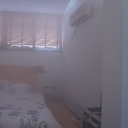
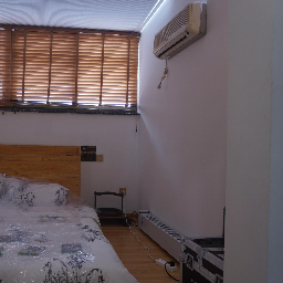
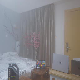
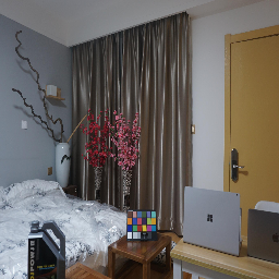
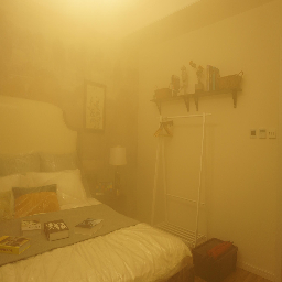
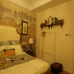
In this experiment, we aim to overcome these limitations and evaluate our method on a subset of bedroom scenes from the REVIDE dataset [32], which contains a total of 240 real hazy image pairs across 9 scenes. This dataset represents an ideal use case for our method, as only a restricted number of paired images are available to train on.

Similar to the in-painting experiment, we train a U-net on 5 paired images and 200+20,000 unpaired images, where the 5 paired and 200 unpaired images are sourced from REVIDE and the additional 20,000 unpaired images are sourced from the LSUN bedrooms dataset [29]. Before training the image reconstruction network, we first pre-train both a diffusion model and a CycleGAN. Specifically, we train the diffusion model on 20,000 non-hazy bedroom images from the LSUN dataset [29] and train CycleGAN on the same LSUN images (along with the 5 paired and 200 unpaired images from REVIDE).

Compared to baselines methods, we find that SUD² produces reconstructions with far fewer artifacts and achieves a median LPIPS score $17\%$ lower than the supervised baseline. Visually, the dehazed images generated by SUD² have a more natural and smooth appearance relative to both CycleGAN and the supervised baseline as shown in Figure 9. In contrast, due to the limited number of hazy training samples, CycleGAN fails to learn a good mapping between hazy and non-hazy images, resulting in poor PSNR, SSIM, and LPIPS scores.

5 Limitations and future work

Our experiments demonstrate that SUD² enables the use of deep learning techniques even when paired data is scarce. Nonetheless, there remain limitations to our approach which can be addressed in future works.

For instance, performance improvements gained from SUD² are directly correlated with the strength of the prior imposed by the unconditional denoising diffusion model. As the target image distribution grows more diverse, the strength of this learned prior weakens. Conditional diffusion models offer a promising avenue for maintaining a strong prior on diverse image distributions that can be explored in future works.

Furthermore, the reconstruction networks produced by the SUD² training procedure are deterministic. Extending SUD² to train stochastic algorithms which produce diverse outputs [10] is another interesting direction for future work.

6 Conclusion

We introduce SUD², a generalized deep learning framework for solving few-shot, semi-supervised image reconstruction problems. Inspired by the recent success of denoising diffusion models on image generation tasks, we leverage diffusion models to regularize network training, encouraging solutions that lie close to the desired image distribution.

To benchmark our method, we apply SUD² on image reconstruction tasks and compare against CycleGAN, a well-studied generative model that utilizes unpaired data to perform image-to-image translation. When applied to image in-painting, we find that our method produces significantly more structured faces than baselines, where each facial feature is proportionately sized and reasonably positioned on the face. Similarly, when applied to image dehazing, we observe that results from our method are far less noisy compared to baseline methods. Based off of both qualitative and quantitative experimental results, SUD² succeeds in enabling the training of deep networks on datasets where few paired data samples are available.

7 Acknowledgements

M.C. and C.M. were supported in part by the AFOSR Young Investigator Program Award FA9550-22-1-0208 and a Northrop Grumman seed grant.

See pages 1 of supplement.pdf See pages 0 of supplement.pdf

References

- [1] Codruta O. Ancuti, Cosmin Ancuti, Radu Timofte, and Christophe De Vleeschouwer. I-haze: a dehazing benchmark with real hazy and haze-free indoor images. In arXiv:1804.05091v1, 2018.
- [2] Codruta O. Ancuti, Cosmin Ancuti, Radu Timofte, and Christophe De Vleeschouwer. O-haze: a dehazing benchmark with real hazy and haze-free outdoor images. In IEEE Conference on Computer Vision and Pattern Recognition, NTIRE Workshop, NTIRE CVPR’18, 2018.
- [3] Bolun Cai, Xiangmin Xu, Kui Jia, Chunmei Qing, and Dacheng Tao. Dehazenet: An end-to-end system for single image haze removal. Trans. Img. Proc., 25(11):5187–5198, nov 2016.
- [4] Hyungjin Chung, Jeongsol Kim, Michael Thompson Mccann, Marc Louis Klasky, and Jong Chul Ye. Diffusion posterior sampling for general noisy inverse problems. In The Eleventh International Conference on Learning Representations, 2023.
- [5] Kostadin Dabov, Alessandro Foi, Vladimir Katkovnik, and Karen Egiazarian. Image denoising by sparse 3-d transform-domain collaborative filtering. IEEE Transactions on image processing, 16(8):2080–2095, 2007.
- [6] Bradley Efron. Tweedie’s formula and selection bias. Journal of the American Statistical Association, 106:1602–1614, 12 2011.
- [7] Karen Egiazarian, Alessandro Foi, and Vladimir Katkovnik. Compressed sensing image reconstruction via recursive spatially adaptive filtering. In 2007 IEEE International Conference on Image Processing, volume 1, pages I–549. IEEE, 2007.
- [8] D. Engin, A. Genc, and H. Ekenel. Cycle-dehaze: Enhanced cyclegan for single image dehazing. In 2018 IEEE/CVF Conference on Computer Vision and Pattern Recognition Workshops (CVPRW), pages 938–9388, Los Alamitos, CA, USA, jun 2018. IEEE Computer Society.
- [9] Jonathan Ho, Ajay Jain, and Pieter Abbeel. Denoising diffusion probabilistic models. Advances in Neural Information Processing Systems, 33:6840–6851, 2020.
- [10] Zahra Kadkhodaie and Eero Simoncelli. Stochastic solutions for linear inverse problems using the prior implicit in a denoiser. Advances in Neural Information Processing Systems, 34:13242–13254, 2021.
- [11] Samuli Laine and Timo Aila. Temporal ensembling for semi-supervised learning. arXiv preprint arXiv:1610.02242, 2016.
- [12] Cheng-Han Lee, Ziwei Liu, Lingyun Wu, and Ping Luo. Maskgan: Towards diverse and interactive facial image manipulation. In IEEE Conference on Computer Vision and Pattern Recognition (CVPR), 2020.
- [13] Dong-Hyun Lee. Pseudo-label : The simple and efficient semi-supervised learning method for deep neural networks. ICML 2013 Workshop : Challenges in Representation Learning (WREPL), 07 2013.
- [14] Christopher A Metzler, Arian Maleki, and Richard G Baraniuk. From denoising to compressed sensing. IEEE Transactions on Information Theory, 62(9):5117–5144, 2016.
- [15] Vinod Nair and Geoffrey E. Hinton. Rectified linear units improve restricted boltzmann machines. In Proceedings of the 27th International Conference on International Conference on Machine Learning, ICML’10, page 807–814, Madison, WI, USA, 2010. Omnipress.
- [16] Srinivasa G. Narasimhan and Shree K. Nayar. Vision and the atmosphere. International Journal of Computer Vision, 48:233–254, 2002.
- [17] Shree K Nayar and Srinivasa G Narasimhan. Vision in bad weather. In Proceedings of the seventh IEEE international conference on computer vision, volume 2, pages 820–827. IEEE, 1999.
- [18] Gregory Ongie, Ajil Jalal, Christopher A Metzler, Richard G Baraniuk, Alexandros G Dimakis, and Rebecca Willett. Deep learning techniques for inverse problems in imaging. IEEE Journal on Selected Areas in Information Theory, 1(1):39–56, 2020.
- [19] Edward T Reehorst and Philip Schniter. Regularization by denoising: Clarifications and new interpretations. IEEE transactions on computational imaging, 5(1):52–67, 2018.
- [20] Wenqi Ren, Si Liu, Hua Zhang, Jinshan Pan, Xiaochun Cao, and Ming-Hsuan Yang. Single image dehazing via multi-scale convolutional neural networks. In Computer Vision–ECCV 2016: 14th European Conference, Amsterdam, The Netherlands, October 11-14, 2016, Proceedings, Part II 14, pages 154–169. Springer, 2016.
- [21] Yaniv Romano, Michael Elad, and Peyman Milanfar. The little engine that could: Regularization by denoising (red). SIAM Journal on Imaging Sciences, 10(4):1804–1844, 2017.
- [22] Olaf Ronneberger, Philipp Fischer, and Thomas Brox. U-net: Convolutional networks for biomedical image segmentation. In Nassir Navab, Joachim Hornegger, William M. Wells, and Alejandro F. Frangi, editors, Medical Image Computing and Computer-Assisted Intervention – MICCAI 2015, pages 234–241, Cham, 2015. Springer International Publishing.
- [23] Alexander Sorokin and David Forsyth. Utility data annotation with amazon mechanical turk. In 2008 IEEE Computer Society Conference on Computer Vision and Pattern Recognition Workshops, pages 1–8, 2008.
- [24] Antti Tarvainen and Harri Valpola. Mean teachers are better role models: Weight-averaged consistency targets improve semi-supervised deep learning results. In Proceedings of the 31st International Conference on Neural Information Processing Systems, NIPS’17, page 1195–1204, Red Hook, NY, USA, 2017. Curran Associates Inc.
- [25] Singanallur V Venkatakrishnan, Charles A Bouman, and Brendt Wohlberg. Plug-and-play priors for model based reconstruction. In 2013 IEEE Global Conference on Signal and Information Processing, pages 945–948. IEEE, 2013.
- [26] Michael B Wakin, David L Donoho, Hyeokho Choi, and Richard G Baraniuk. High-resolution navigation on non-differentiable image manifolds. In Proceedings.(ICASSP’05). IEEE International Conference on Acoustics, Speech, and Signal Processing, 2005., volume 5, pages v–1073. IEEE, 2005.
- [27] Xiangli Yang, Zixing Song, Irwin King, and Zenglin Xu. A survey on deep semi-supervised learning. IEEE Transactions on Knowledge and Data Engineering, 2022.
- [28] Sean I Young, Adrian V Dalca, Enzo Ferrante, Polina Golland, Bruce Fischl, and Juan Eugenio Iglesias. Sud: Supervision by denoising for medical image segmentation. arXiv preprint arXiv:2202.02952, 2022.
- [29] Fisher Yu, Ari Seff, Yinda Zhang, Shuran Song, Thomas Funkhouser, and Jianxiong Xiao. Lsun: Construction of a large-scale image dataset using deep learning with humans in the loop. arXiv preprint arXiv:1506.03365, 2015.
- [30] Kai Zhang, Wangmeng Zuo, Yunjin Chen, Deyu Meng, and Lei Zhang. Beyond a gaussian denoiser: Residual learning of deep cnn for image denoising. IEEE transactions on image processing, 26(7):3142–3155, 2017.
- [31] R. Zhang, P. Isola, A. A. Efros, E. Shechtman, and O. Wang. The unreasonable effectiveness of deep features as a perceptual metric. In 2018 IEEE/CVF Conference on Computer Vision and Pattern Recognition (CVPR), pages 586–595, Los Alamitos, CA, USA, jun 2018. IEEE Computer Society.
- [32] Xinyi Zhang, Hang Dong, Jinshan Pan, Chao Zhu, Ying Tai, Chengjie Wang, Jilin Li, Feiyue Huang, and Fei Wang. Learning to restore hazy video: A new real-world dataset and a new method. In Proceedings of the IEEE/CVF Conference on Computer Vision and Pattern Recognition (CVPR), pages 9239–9248, June 2021.
- [33] Jun-Yan Zhu, Taesung Park, Phillip Isola, and Alexei A Efros. Unpaired image-to-image translation using cycle-consistent adversarial networks. In Computer Vision (ICCV), 2017 IEEE International Conference on, 2017.