Neural Architecture Search for Effective Teacher-Student Knowledge Transfer in Language Models

Abstract

Large pretrained language models have achieved state-of-the-art results on a variety of downstream tasks. Knowledge Distillation (KD) into a smaller student model addresses their inefficiency, allowing for deployment in resource-constrained environments. However, KD can be ineffective when the student is manually selected from a set of existing options, since it can be a sub-optimal choice within the space of all possible student architectures. We develop multilingual KD-NAS, the use of Neural Architecture Search (NAS) guided by KD to find the optimal student architecture for task agnostic distillation from a multilingual teacher. In each episode of the search process, a NAS controller predicts a reward based on the distillation loss and latency of inference. The top candidate architectures are then distilled from the teacher on a small proxy set. Finally the architecture(s) with the highest reward is selected, and distilled on the full training corpus. KD-NAS can automatically trade off efficiency and effectiveness, and recommends architectures suitable to various latency budgets. Using our multi-layer hidden state distillation process, our KD-NAS student model achieves a 7x speedup on CPU inference (2x on GPU) compared to a XLM-Roberta Base Teacher, while maintaining 90% performance, and has been deployed in 3 software offerings requiring large throughput, low latency and deployment on CPU.

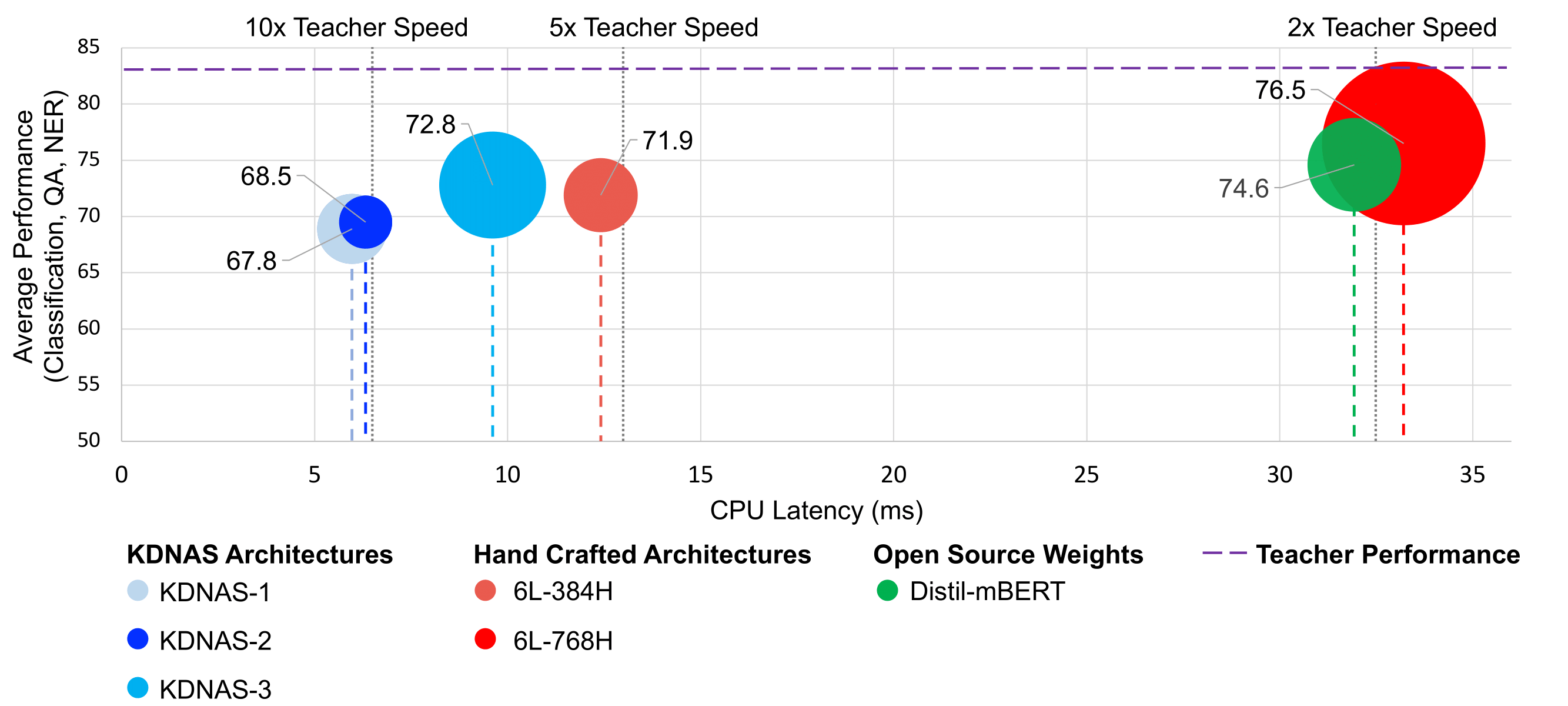
Figure 1: KD-NAS architectures compared to hand-crafted baselines (bubble size indicates total parameters). At similar performance, KD-NAS selects faster architectures. At similar latency, architectures distilled on our pipeline outperform open-source baselines.

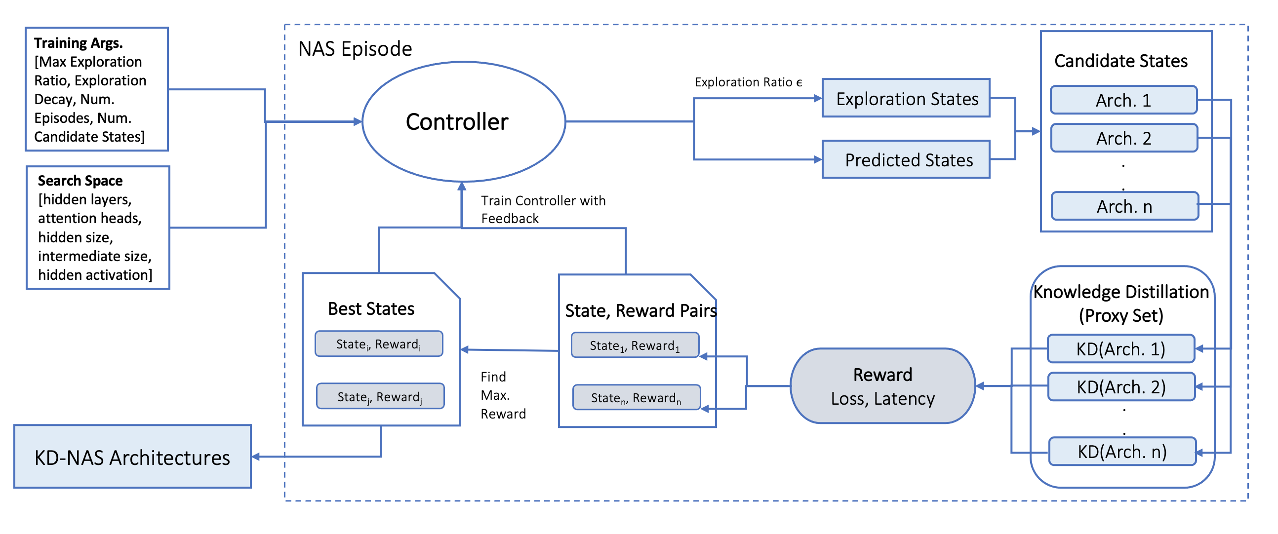
Figure 2: KD-NAS. In each episode, the controller predicts the states with the highest reward. These states are chosen as candidate architectures to be distilled from the teacher in a reduced-KD process. The actual reward is obtained, and is used to train the controller, along with a memory of previously explored high performing states.

1 Introduction

Pretrained language models Devlin et al. (2019); Liu et al. (2019b); Clark et al. (2020b); Conneau et al. (2020) are capable of showing extraordinary performance on a variety of downstream language tasks. However, such models have a large number of parameters Vaswani et al. (2017); Devlin et al. (2019); Liu et al. (2019b); Brown et al. (2020); Kaplan et al. (2020); Fedus et al. (2021), requiring huge amounts of memory to be deployed. Additionally, they have a large latency for inference - making them inefficient to deploy in resource-constrained environments, or in products that require a large throughput, low latency and low memory footprint. Smaller models may be more suitable for use in practice, but often sacrifice performance for the sake of deployment Huang et al. (2015). Moreover, these models are ineffective due to their hand-crafted architecture design - in the space of all possible architectures given a certain resource budget, manual selection is likely sub-optimal even if guided by human expertise, and selecting the optimal architecture through trial-and-error for various latency budgets can be prohibitively expensive.

Knowledge Distillation (KD) Hinton et al. (2015) trains a smaller student model to mimic a larger teacher model. This improves the efficiency of current models, making the compressed model suitable for deployment without losing much performance. In practice, having a manually designed student with layers initialized from the teacher can be immensely beneficial to the distillation process Wang et al. (2023); Sanh et al. (2020); Turc et al. (2019), but this puts a constraint on the architecture of the student. However, an optimal student architecture may exist, given a specific teacher model Liu et al. (2020). This motivates us to focus on architecture-agnostic distillation methods for student models which can have different architectural parameters from the teacher. Specifically, we follow a task-agnostic hidden state distillation objective Jiao et al. (2020, 2021); Mukherjee et al. (2021); Ko et al. (2023), and improve the performance of a multilingual student model without pre-training or initialization from the teacher. Moreover, we use Neural Architecture Search (NAS) Elsken et al. (2019); Zoph and Le (2017); Liu et al. (2019a); So et al. (2019) to efficiently automate the process of finding the best transformer architecture optimized for distilling knowledge from a multilingual teacher, obtaining faster architectures for a given performance level (Fig. 1). Our key contributions are:

• We develop KD-NAS, a system that improves the NAS process to identify an optimal yet efficient architecture from a pre-defined search space for a general purpose modelling objective. KD-NAS incorporates a KD objective with the traditional loss and latency measures into the NAS Reward. We introduce a Feedback Controller to guide the search process, which draws on information from the top performing states explored in previous episodes.

• We propose a multi-layer hidden state distillation approach, in which each student layer learns the internal representations of two teacher layers, allowing for the transfer of both low-level and high-level knowledge. This method effectively transfers knowledge without pre-training or weight initialization.

• We demonstrate how KD-NAS recommended architectures have been deployed for low-latency applications, achieving significant speedup while maintaining 90% of teacher performance.

2 Background

Knowledge Distillation

KD is a method of model compression in which the knowledge of a large model is transferred to a student through transferring its internal representations or outputs Ba and Caruana (2014); Hinton et al. (2015). In transformer language models Vaswani et al. (2017), prior work has distilled teacher outputs Hinton et al. (2015); Sanh et al. (2020); Jafari et al. (2021), hidden states Mukherjee et al. (2021); Sun et al. (2019); Jiao et al. (2021); Li et al. (2020), multi-head self-attentions Zagoruyko and Komodakis (2017); Wang et al. (2020, 2021), or a combination of the above Sanh et al. (2020); Mukherjee et al. (2021).

This work adopts architecture-agnostic Hidden State (HS) distillation methods based on linear projections Mukherjee et al. (2021); Jiao et al. (2020), in which a student is trained to learn the representations of the teacher’s hidden state. Formally, for models with $L$ Transformer layers, the hidden state of the $i^{th}$ layer is $\mathbf{H}_{i}\in\mathbb{R}^{|x|\times d_{h}}$, where $d_{h}$ is the hidden size and $|x|$ is the sequence length. For HS Distillation from a teacher with $L^{T}$ layers to a student with $L^{S}$ layers (with hidden size ${d}^{T}_{h}$ and ${d}^{S}_{h}$ respectively), we map the $i^{th}$ student layer to a set of teacher layers, $g(i)$. For each $j\in g(i)$, we linearly transform the hidden state of the student $\mathbf{H}^{S}_{j}\in\mathbb{R}^{|x|\times{d}^{S}_{h}}$ using a learnable projection matrix $\mathbf{W}^{j}_{i}\in\mathbb{R}^{{d}^{S}_{h}\times{d}^{T}_{h}}$, and train the student to predict the hidden state of the teacher $\mathbf{H}^{T}_{j}\in\mathbb{R}^{|x|\times{d}^{T}_{h}}$ using the Mean Squared Error (MSE) loss:

$$\mathcal{L}_{\mathrm{HS}}(S,T)=\sum_{i=1}^{L^{S}}\sum_{j\in g(i)}\mathrm{MSE}\Bigl{(}\mathbf{H}^{S}_{j}\mathbf{W}_{i}^{j},\mathbf{H}^{T}_{j}\Bigl{)}$$ (1)

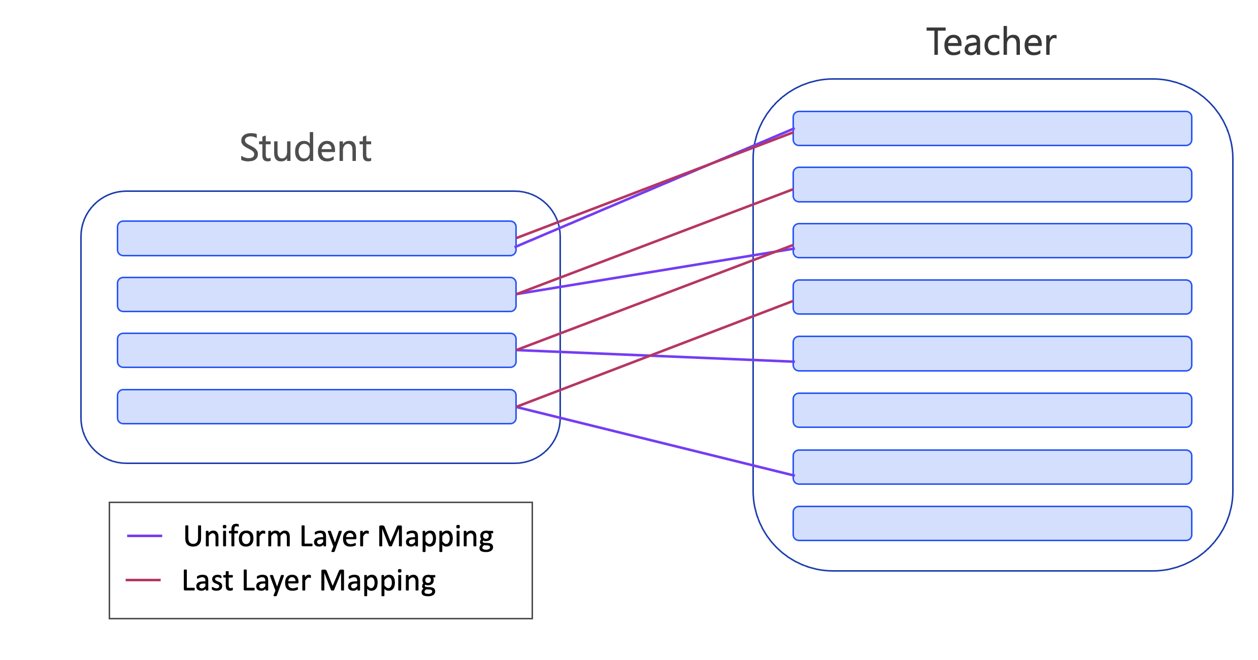
Figure 3: Multi-layer mapping for HS Transfer. Lines from teacher layers to a student layer $i$ graphically depict the mapping function $g(i)$.

This work proposes a multi-layer mapping strategy Jiao et al. (2021); Wu et al. (2021), where each student layer learns from two teacher layers, as illustrated in Fig. 3. This allows the student to learn both high-level (e.g. semantic) and low level (e.g. syntactic) knowledge in the teacher representations Tenney et al. (2019). Specifically we set $|g(i)|=2$ for $i\in[1,L^{S}]$, and combine the Uniform (or "skip") Jiao et al. (2020); Sun et al. (2019) and Last Mukherjee et al. (2021) strategies commonly used for KD where $L^{T}>L^{S}$:

$$g(i)=\{(i-1)\left\lceil\dfrac{L^{T}}{L^{S}}\right\rceil+1,L^{T}-L^{S}+i\}\\$$ (2)

We compare this method to common layer mapping strategies for HS distillation in Appendix A.

Neural Architecture Search

NAS automates the process of selecting the best candidate architecture for a given task. The search space defines the set of possible candidate architectures. For a transformer model, this may include components of the transformer architecture. The goal of NAS is to pick within the the search space an architecture which performs optimally, using a search strategy which makes the process more efficient than a brute-force search. NAS typically employs algorithms such as Reinforcement Learning Zoph and Le (2017); Zoph et al. (2018); Tan et al. (2019), Evolutionary Algorithms So et al. (2019) or Differential Search Liu et al. (2019a) in order to optimize the search process over a large, multi-dimensional search space. Since training candidate architectures on the entire target pipeline is computationally expensive, a common performance evaluation strategy is to conduct only a portion of the training on a "proxy set" Liu et al. (2019a); Zhou et al. (2020); Na et al. (2021). This constitutes training on a reduced version of the corpus for a limited number of epochs, and must be representative of the performance on the entire training pipeline.

3 KD-NAS: KD Aware Neural Architecture Search

We describe the design of our KD guided NAS process (KD-NAS), which uses NAS to find the optimal student architecture for task-agnostic distillation from a given teacher. Fig. 2 shows the overall process.

Parameter Candidate Values Hidden Layers [3, 4, 6, 10, 12] Attention Heads [2, 3, 4, 6, 12] Intermediate Size [384, 512, 576, 768, 1024, 1536, 2048, 3072] Hidden Activation [gelu, relu, silu]

Table 1: Search Space Candidates for KD-NAS, consisting of 2400 student architectures.

Search Space

We define a five-dimensional search space for the student transformer model, comprising of the number of hidden layers, number of attention heads, hidden size, intermediate (FFN) size, and hidden activation function, as shown in Table 1. This space includes 2400 possible student architectures. Note, in this work we use the terms state and architecture interchangeably.

Performance Evaluation System

To estimate the reward, each candidate student model is distilled from the teacher on a proxy set. We define a 4-epoch mini-KD process, using 30% of the training corpus. This reduces the time to distil each student, thus being a practical method of evaluating multiple candidate architectures. We obtain this choice of proxy set by experimenting with different combinations of data size and training epochs, and select the smallest process that maintains the relative ranking of distillation loss for a set of randomly selected architectures from the search space.

Search Strategy

This work implements a reinforcement learning based approach for NAS, with the following components:

A. Feedback Controller

We train a Long Short Term Memory (LSTM) Hochreiter and Schmidhuber (1997); Bakker (2002) Controller model to predict the reward given a state and a memory of performance of previously explored states. Specifically, in each NAS episode $ep_{n}$, we pass as input the current state being explored, and two additional states: the Global Best State (the highest-reward architecture from all prior episodes $ep_{i\in[1,n-1]}$), and the Previous Best State (the highest-reward architecture from episode $ep_{n-1}$).

B. Search Mechanism

Each episode of KD-NAS comprises of the following steps:

1. Each episode generates $N$ candidate states, including those selected by the controller and those selected for random exploration. Initially, the controller benefits from more exploration of the search space, which is controlled by the exploration ratio $\epsilon$. We decay $\epsilon_{1}=1$ to $\epsilon_{min}=0.05$ with a decay rate of $0.05$ per episode.

2. The mini-KD process is performed for each candidate state $s$, to obtain the reward $reward(S_{s})$ of the resulting distilled student $S_{s}$.

3. The (state,reward) pairs are concatenated with (GlobalBestState, PreviousBestState) and is used as training data to minimize the Controller loss $L_{C}$, i.e, the MSE between the actual reward of the model after distillation on the proxy set, $reward(S_{s})$, and the predicted reward $reward_{pred}(s)$ for all states $s$ belonging to the candidate states $CS$ of that episode:

   $$L_{C}=\frac{1}{2}\sum_{s\in CS}\|reward(S_{s})-reward_{pred}(s)\|^{2}$$ (3)

This process is repeated for $M$ episodes, after which the explored architectures with the highest reward are selected.

C. Reward Function

The reward is a function of the student’s latency of inference on a CPU $lat(S_{s})$, and the distillation loss $\mathcal{L}_{\mathrm{HS}}$ (Eq. 1) between the student $S_{s}$ and teacher $T$. The latency is normalized using the maximum target latency, i.e., a fraction of the teacher latency $lat(T)$. The reward is similar to the optimization goal of Tan et al. (2019):

$$reward(S_{s})=(1-\mathcal{L}_{\mathrm{HS}}(S_{s},T))\cdot\left(\frac{lat(S_{s})}{\beta*lat(T)}\right)^{\alpha}$$ (4)

The hyperparameters $\alpha$ and $\beta$ control the relative weight of latency in the optimization goal, and the maximum target latency respectively.

4 Experiments and Results

Model Architecture Params Latency (ms) $\downarrow$ (M) CPU GPU KDNAS_Arch1 3,12,384,1024,gelu 100 5.97_±0.04 3.25_±0.01 KDNAS_Arch2 4,4,288,768,gelu 76 6.12_±0.03 3.49_±0.02 KDNAS_Arch3 4,12,576,768,gelu 153 9.19_±0.03 3.98_±0.02 6L-384H^$\dagger$ 6,12,384,1536,gelu 107 12.41_±0.03 5.99_±0.07 6L-768H^$\dagger$ 6,12,768,3072,gelu 234 33.21_±0.07 6.01_±0.06 DistilBERT 6,12,768,3072,gelu 134 30.93_±0.03 5.64_±0.04 Teacher 12,12,768,3072,gelu 277 64.98_±0.51 9.47_±0.01

Table 2: Model Architectures, depicted as [hidden layers, attention heads, hidden size, intermediate size, activation function]. Latency measured on an A100 GPU and 4-core CPU, over 3 runs. ^†architectures distilled on our pipeline.

Baselines

For a fair analysis of our technique, we compare our NAS-recommended architectures to two popular student architectures- a 6 layer, 768 hidden size (6L-768H) architecture Sanh et al. (2020), and a smaller 6 layer, 384 hidden size (6L-384H) architecture Wang et al. (2020); Mukherjee et al. (2021); Wang et al. (2021), distilled on our own pipeline. We compare the architecture of our KD-NAS models with common open source baselines, and demonstrate an optimal trade-off between speed and performance with our models. Additionally, we compare our architectures and distillation method to the popular open source Multilingual Distil-BERT model. These architectures, along with those recommended by KD-NAS, are described in Table 2.

4.1 KD-NAS Implementation

Data

We conduct a multilingual, task-agnostic distillation to produce general purpose students, on a subset of 7M sentences from the multilingual CC100 dataset Conneau et al. (2020).

Architecture Search

We conduct KD-NAS to find the best student architecture to distil from an in-house XLM-Roberta Base Conneau et al. (2020) teacher over $15$ episodes (each producing $20$ candidate architectures) using the proxy set mini-KD as an estimation of distillation loss. KD-NAS is guided by the reward function Eq. 4, with $\alpha=-0.06$, $\beta=0.6$. For consistent and comparable latency measurements, we create a lookup table of the latencies of all randomly-initialized students on a single CPU.

We obtain the top $3$ architectures recommended by the KD-NAS process, (KDNAS_Arch1, KDNAS_Arch2, KDNAS_Arch3), with different latency budgets, as described in Table 2. To evaluate the efficacy of our NAS system, we compare it to random sampling over the defined search space Yang et al. (2020). The average loss, latency, and reward after the distillation of 3 randomly selected student architectures over 3 seeds have been shown in Table 3. As seen, KD-NAS models outperform the random sampling models in all metrics, encouraging the use of NAS over random sampling.

Model Distillation CPU Reward Loss$\downarrow$ Latency (ms)$\downarrow$ $\uparrow$ Random_Seed1 0.051_±0.01 13.20_±6.0 1.02_±0.03 Random_Seed2 0.050_±0.01 11.40_±3.6 1.03_±0.02 Random_Seed3 0.057_±0.01 14.17_±3.1 1.01_±0.02 KDNAS_Arch1 0.050 5.97 1.07 KDNAS_Arch2 0.049 6.12 1.07 KDNAS_Arch1 0.043 9.19 1.05

Table 3: Random Sampling vs KD-NAS. Avg. metrics shown for 3 random architectures per seed for 3 seeds.

Model Params Latency $\downarrow$ Monolingual Performance $\uparrow$ Multilingual Performance $\uparrow$ Avg. $\uparrow$ (M) CPU GPU GLUE SQuAD CoNLL XNLI TyDi NER^$\star$ KDNAS_Arch1 100 5.97 3.25 76.1_±0.6 55.5_±0.3 90.0_±0.1 57.9_±0.5 56.3_±0.4 71.3_±0.1 67.9 KDNAS_Arch2 76 6.12 3.49 76.1_±0.3 56.9_±0.2 90.0_±0.3 58.3_±0.6 58.7_±0.3 72.0_±0.4 68.6 KDNAS_Arch3 153 9.19 3.98 79.6_±0.6 62.7_±0.1 92.1_±0.2 62.7_±0.5 66.8_±0.6 72.8_±0.1 72.8 6L-384H^$\dagger$ 107 12.41 5.99 78.7_±0.8 62.4_±0.1 91.4_±0.2 62.7_±0.4 63.4_±0.5 73.1_±0.1 71.9 6L-768H^$\dagger$ 234 33.21 6.01 83.1_±0.3 68.0_±0.3 93.9_±0.1 67.0_±0.4 72.7_±0.6 74.2_±0.1 76.5 DistilBERT 134 30.93 5.64 81.4_±0.5 68.9 _±0.4 94.2_±0.1 59.4_±0.5 69.8_±0.2 74.2_±0.1 74.7 Random_Seed1 115 13.20 5.31 62.6_±6.2 43.6_±0.9 86.3_±7.6 56.2_±5.7 49.3_±13.14 70.9_±3.6 61.5 Random_Seed2 123 11.40 5.89 76.1_±3.8 56.1_±9.2 89.1_±1.0 60.6_±5.3 61.0_±4.0 71.6_±0.7 69.1 Random_Seed3 91 14.17 6.38 66.5_±3.0 44.5_±2.0 88.6_±3.1 58.0_±1.8 53.9_±5.3 72.5_±1.4 64.1 Teacher 277 64.98 9.47 84.8_±0.3 77.3_±0.5 94.2_±0.1 70.9_±0.8 78.1_±0.7 76.1_±0.1 80.2

Table 4: KD-NAS performance, compared to baselines and random sampling. We report avg. GLUE score across all tasks, avg. XNLI score across all languages, and F1 score of SQuAD, TyDi and CoNLL. Latency measured in ms for an A100 GPU and 4-core CPU. Results shown as avg. across 3 runs. (^†baselines distilled on our pipeline, ^⋆internal dataset)

4.2 Results

After obtaining the KD-NAS recommendations, we distil the models over the entire training pipeline, with the objective described in Eq. 1, to obtain general purpose models. We finetune these models on both monolingual (English) and multilingual benchmarks, and on tasks including text classification (GLUE Wang et al. (2019), XNLI Conneau et al. (2018)), Question Answering (SQuAD Rajpurkar et al. (2016), TyDiQA Clark et al. (2020a)), and Named Entity Recognition (CoNLL Tjong Kim Sang and De Meulder (2003)). We also evaluate on an internal dataset for multilingual Named Entity Recognition, which consists of $17$ entities across $24$ languages (a detailed description of this dataset is given in Appendix D).

We report our results in Table 4, which shows our KD-NAS- recommended models have the least latency of inference on both CPU and GPU, while maintaining good performance. Specifically,

• Our best performing model, KDNAS_Arch3, obtains equivalent or better performance to our 6L-384H baseline on all tasks, while being significantly faster.

• Compared to the 6L-768H architectures, our models show a slight degradation in performance, however, they show a significant gain in speed. Moreover, the average performance of random sampling from the search space is always sub-optimal compared to the KD-NAS models. Thus, KD-NAS can automatically find an optimal trade-off between effectiveness and efficiency, which is expensive to do manually.

• Our proposed multi-layer HS distillation method outperforms multilingual DistilBERT, with the most significant gains seen for multilingual tasks, demonstrating the advantage of transferring the knowledge from multiple teacher layers to each student layer. Notably, this method achieves good results without the need of pre-training (which is computationally expensive) or initializing layers from the teacher (which constrains the architecture).

5 Applications

$KDNAS_{Arch3}$, which we refer to as the Piccolo Architecture, is significantly faster than the teacher, while maintaining good performance. After further experiments, we find that distilling the self-attention relations as proposed in MiniLM-v2 Wang et al. (2021) improves performance Udagawa et al. (2023). We use this distillation objective to produce a model that has been deployed for natural language understanding applications requiring low latency and high throughput, namely:

• Low Latency NLP: after being finetuned on downstream tasks (e.g. entity extraction, sentiment analysis, relation detection) the Piccolo model provides a 7.6x speedup on CPU (2.5x on A100 GPU) relative to the 12-layer teacher, while retaining 93% performance on average. It also results in a 5.9x speedup in finetuning time on average. This allows easy deployment on CPU, edge devices, or low-latency GPU applications, and has been deployed as part of 3 software offerings Lang (2023); Heidloff (2023).

• Hate/Abuse/Profanity (HAP) filtering for data pre-processing: Language models are trained on data originating from internet sources, which may contain profane language. Using uncivil content for training may lead to the model producing similar hateful content as well, which is not suitable for business use. The Piccolo Model, finetuned to identify hate-speech Poletto et al. (2021), is used to efficiently filter a large corpus of training data for HAP. Using this model results in faster inference (7x on CPU, 2x on GPU), larger throughput (3.5x) and a lower memory consumption (4x fewer parameters) than a 12-layer model, while maintaining equivalent performance, and has been deployed in internal and external software offerings.

6 Related Work

Our work is most comparable to prior work that uses KD to guide NAS for language models. AdaBERT Chen et al. (2021) compresses monolingual BERT models into models using differentiable NAS that also combines a distillation loss into the search objective. However, they conduct their search in a task-specific manner, where the KD loss is determined by using probes to hierarchically decompose the task-useful knowledge from the teacher model, and then distilling it. While this may be able to achieve a higher compression rate, is not effective for producing general purpose students that can be further finetuned on task-specific data, which are more useful in industrial settings. NAS-BERT Xu et al. (2021) produces task-agnostic, compressed monolingual BERT models for different latency budgets, by training a large supernet using block-wise training. While each block of the supernet is trained using KD to mimic the corresponding teacher block, we use KD explicitly to guide the search process and formulate the NAS reward, and conduct our search on the entire student architecture. Moreover, our Feedback Controller model determines the next states to be explored by predicting the rewards of the given state along with information regarding well-performing states seen in the past, which is a contrast from the probabilistic actor-critic agent proposed in previous work Liu et al. (2020); Bashivan et al. (2019); Wang (2021). While most prior art focuses on monolingual (English) models, we expand search to the multilingual domain in a task-agnostic setting.

7 Conclusion

We develop KD-NAS, a method to non-trivially adopt NAS to optimize for the KD objective, thus transferring task-agnostic knowledge from a large model into an optimal architecture within a large search space. After distillation, our KD-NAS models show significant speedup over a hand-crafted baseline while maintaining performance. Larger students distilled with our task-agnostic multi-layer hidden state transfer objective outperforms an open-source model with the same architecture. We illustrate how a high performing KD-NAS model has been deployed for low-latency applications.

Appendix A Hidden State Distillation

This work presents a multi-layer hidden state distillation approach, where each student layer learns from two teacher layers. While transferring hidden states, the choice of layer mapping is key, and is often a controversial choice Wu et al. (2020); Jiao et al. (2021); Ko et al. (2023). Here, we compare single-layer mapping strategies (where a student layer is mapped to only one teacher layer) with our Uniform+Last multi-layer mapping strategy when distilling the 6L-768H student baseline. The single-layer mapping strategies studied are

1. Last-1: we distil the last teacher layer into the last student layer.

2. Last: we map each student layer $i$ to the last $i^{th}$ teacher layer Mukherjee et al. (2021).

3. Uniform: we choose every $k^{th}$ teacher layer, where $k=\lceil L^{T}/L^{S}\rceil$ (also known as the "skip" strategy) Sanh et al. (2020); Sun et al. (2019).

We evaluate the distilled students on the GLUE benchmark Wang et al. (2019) and the XNLI task Conneau et al. (2018). The results in Table 6 show the proposed Uniform+Last strategy outperforming all single layer mapping strategies, as it allows for the transfer of diverse knowledge from the teacher.

Appendix B Training Details and Hyperparameters

Dataset bsz lr epochs GLUE (-CoLA) 32 2e-5 3 CoLA 32 2e-5 10 SQuAD 32 3e-5 6 CoNLL 32 5e-5 3 XNLI 32 2e-5 5 TyDi 32 1e-5 10 NER^$\star$ 32 5e-5 5

Table 5: Hyperparameters for Finetuning (batch size, learning rate, and finetuning epochs). (^⋆internal dataset)

Teacher Training

We follow the training procedure of XLM-Roberta Conneau et al. (2020), and train the Base model (12 layers) on the CC100 dataset Conneau et al. (2020). We use a peak learning rate of $6e-4$, the Adam optimizer with polynomial decay (with a warmup of 72K steps) and train the model for $1.5$ million steps, on a masked language modelling (MLM) objective with a masking probability of $0.15$.

Hidden State Distillation

We distill our KD-NAS recommended architectures on a subset of the CC100 dataset (with data in 116 languages) used to train the teacher. We train for $130,000$ steps, using an AdamW Optimizer Loshchilov and Hutter (2019) (with $\beta_{1}=0.9,\beta_{2}=0.98$). We use a peak learning rate of $8e-4$ with a linear LR schedule with a warmup of 6.5K steps. We use a batch size of $32$ and train on 2 NVIDIA A100 GPUs.

KD-NAS Pipeline

Our KD-NAS controller is a single layer LSTM with $32$ cells, and is trained for 10 epochs per episode. We use a RMSProp optimizer Tijmen and Hinton (2012) (with $\gamma=0.95$), a peak learning rate of $1e-4$ and an exponential learning rate schedule. For the proxy-set distillation, we follow the same parameters described above, except that we train for $4$ epochs on $30\%$ of the distillation data. We use a batch size of $32$ and distil on 1 NVIDIA A100 GPU.

Layer GLUE XNLI Mapping MNLI QQP QNLI SST-2 CoLA STS-B MRPC RTE Avg. Avg. (-CoLA) Avg. Last-1 77.6 85.9 85.2 88.5 25.1 84.8 86.2 57.3 73.8(0.7) 80.8(0.6) 56.2(0.4) Last 79.4 86.3 86.6 89.2 25.8 83.3 85.1 62.1 74.7(1.0) 81.7(0.9) 63.1(0.4) Uniform 78.8 85.9 86.0 89.4 26.2 84.0 87.3 60.0 74.7(0.8) 81.6(0.5) 59.9(0.6) Uniform+Last 80.8 86.8 87.9 90.2 32.3 84.7 88.5 62.6 76.7(0.6) 83.1(0.3) 67.0(0.4)

Table 6: Layer Mapping Strategies for Hidden State KD for the 6L-768H Student. Average scores reported over 3 seeds (standard deviation in parenthesis). Best results in bold.

Model GLUE MNLI QQP QNLI SST-2 CoLA STS-B MRPC RTE Avg. Avg. (-CoLA) KDNAS_Arch1 71.0 80.6 81.8 85.9 7.7 76.5 82.6 54.3 67.6(0.7) 76.1(0.6) KDNAS_Arch2 72.7 82.4 82.7 84.9 12.6 71.6 81.7 56.6 68.2(0.5) 76.1(0.3) KDNAS_Arch3 76.5 84.1 84.5 88.1 18.6 82 82.4 59.1 71.9(0.8) 79.5(0.6) 6L-384H^$\dagger$ 76.1 83.7 83.8 87.5 17.8 78.2 84.4 57.3 71.1(1.0) 78.7(0.8) 6L-768H^$\dagger$ 80.8 86.8 87.9 90.2 32.3 84.7 88.5 62.6 76.7(0.6) 83.1(0.3) DistilBERT 78.8 85.9 86.9 88.9 29.1 84.5 87.9 60.4 75.3(0.6) 81.4(0.5) Random_Seed1 64.4 72.4 65.1 85.2 14.9 17.6 81.2 52.2 56.6(6.5) 62.6(6.2) Random_Seed2 74.3 82.6 83.3 87.4 16.9 66.4 83.7 55.8 68.7(3.2) 76.1(3.8) Random_Seed3 67.7 73.8 64.8 86.1 17.4 36.5 81.1 55.2 60.3(2.0) 66.5(3.0) Teacher 84.1 87.9 90.2 91.9 51.7 86.6 91.4 61.4 80.6(0.3) 84.8(0.3)

Table 7: Performance on the GLUE Benchmark. Average taken over three seeds, standard deviation in parenthesis.

Model XNLI ar bg de el en es fr hi ru sw th tr ur vi zh Avg. KDNAS_Arch1 55.0 61.6 60.8 59.5 72.8 62.6 61.5 52.0 57.5 46.7 54.1 55.9 50.7 60.4 57.8 57.9 (0.5) KDNAS_Arch2 55.9 62.1 61.2 61.9 73.2 62.7 62.0 52.7 57.2 45.9 57.3 54.9 48.5 59.9 58.9 58.3(0.6) KDNAS_Arch3 58.8 64.8 63.8 64.4 76.4 68.2 65.5 58.2 64.1 48.8 62.6 58.7 55.9 65.1 64.6 62.7(0.6) 6L-384H^$\dagger$ 59.7 67.2 63.4 65.6 75.9 68.7 66.8 58.3 62.4 48.9 62.7 59.1 53.4 63.2 65.1 62.7 (0.4) 6L-768^$\dagger$ 64.7 69.7 69.6 69.2 80.7 72.0 70.2 64.6 67.7 51.2 65.3 62.5 58.9 70.4 68.6 67.0 (0.4) DistilBERT 58.3 59.7 66.1 58.9 78.9 70.2 67.9 52.9 63.2 47.7 37.1 55.5 52.7 56.9 64.7 59.4 (0.5) Random_Seed1 53.3 59.9 58.1 57.8 69 58.8 58 51.5 59.3 43.5 56 53.9 48.5 57.9 57.9 56.2 (5.7) Random_Seed2 56.5 62 64.2 61.8 75.9 66.5 65.1 55.2 62.1 47.4 61.1 55.4 52.0 63.8 62.2 60.6(5.3) Random_Seed3 54.3 60.4 61.9 59.0 72.0 61.2 60.5 54.2 60.4 43.7 57.8 55.6 50.3 58.9 60.4 58.0(1.8) Teacher 69.1 73.2 74.1 72.2 83.4 75.1 73.1 69 71.3 57.3 69.7 67.7 64.1 70.8 73.3 70.9 (0.8)

Table 8: Performance on the XNLI Task. Average taken over three seeds, standard deviation in parenthesis.

Finetuning Hyperparameters

To finetune our models, we did a coarse grid search on learning rate {$1e-5,2e-5,3e-5,5e-5$} and number of finetuning epochs {$3,5,10$} for a few models, and found that the hyperparameters shown in Table 5 generally work well across models. However, for our internal NER dataset, the teacher model requires $6$ epochs with a learning rate of $5e-6$. We also find finetuning on CoLA for a longer number of epochs particularly helpful for smaller models.

Appendix C Text Classification Results

We show performance of our KD-NAS models and Baselines on all tasks of the GLUE Benchmark, comprising of English text classification tasks in Table 7. We show the per-language performance of the models on XNLI, a cross lingual inference task, trained on English and evaluated on 15 languages in Table 8.

Appendix D Internal Named Entity Recognition Dataset

We use an internal multilingual Named Entity Recognition Dataset to evaluate our models, which contains of $17$ entities across $24$ languages. This set comprises of training set of 518K examples, a development set of 54K examples and a test set of 59K examples. The per-language distribution of training examples is shown in Fig. 4. On average, each training example consists of around 79 words, and about 9 entity mention spans. We show the distribution of these entities across the training set in Fig. 5.

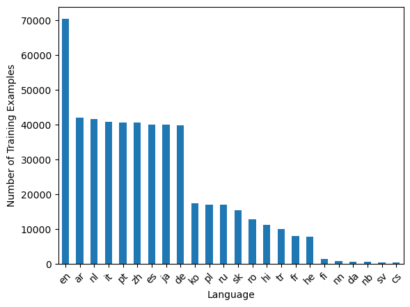
Figure 4: Per-language distribution of training examples for our internal multilingual NER dataset.

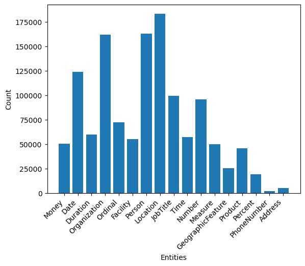
Figure 5: Distribution of entities in training set for our internal multilingual NER dataset.

Model Distillation Monolingual Performance Multilingual Performance Average Algorithm GLUE SQuAD CoNLL XNLI TyDi NER^$\star$ KDNAS_Arch3 HS Transfer 79.5(0.6) 62.7(0.1) 92.1(0.2) 62.7(0.5) 66.8(0.6) 72.8(0.06) 72.8 KDNAS_Arch3 MiniLM 80.7(0.9) 67.4(0.5) 92.5(0.1) 65.3(0.8) 68.6(0.3) 74.2(0.05) 74.8 Teacher 84.8(0.3) 77.3(0.5) 94.2 (0.1) 70.9 (0.8) 78.1(0.7) 76.1(0.06) 80.2

Table 9: Performance of distilling the Piccolo Model (KDNAS_Arch3). Avg. GLUE score across all tasks (except CoLA). Avg XNLI accuracy for all languages. F1 score reported for SQuAD, TyDi and CoNLL. Results shown as an average over 3 seeds, with the average standard deviation shown in parenthesis. ( ^⋆internal dataset)

Appendix E MiniLMv2 Distillation Performance

MiniLM v2 Wang et al. (2021) proposes to train the student model to match the self attention relations of the teacher. Formally, let $d_{h}$ denote the hidden size, and $A_{h}$ denote the number of attention heads of a transformer with $L$ layers, and $|x|$ be the sequence length. We first individually concatenate each of the Query, Key and Value vectors $\mathbf{Q}_{i,a},\mathbf{K}_{i,a},\mathbf{V}_{i,a}\in\mathbb{R}^{|x|\times\frac{d_{h}}{A_{h}}}$ $(a\in[1,A_{h}])$ for layer $i$. They are then split into $A_{r}$ relation heads $\mathbf{A}_{Q,i,r},\mathbf{A}_{K,i,r},\mathbf{A}_{V,i,r}\in\mathbb{R}^{|x|\times d_{r}}$ ($r\in[1,A_{r}]$ and $d_{r}=\frac{d_{h}}{A_{r}}$). The self-attention relations are the scaled dot products of these matrices, or

$$\textbf{R}_{\alpha\beta,i,r}=\mathrm{softmax}\Bigl{(}\frac{\mathbf{A}_{\alpha,l,r}\cdot\mathbf{A}_{\beta,l,r}^{\mathsf{\,T}}}{\sqrt{d_{r}}}\Bigl{)}$$ (5)

Where $\alpha,\beta\in\{Q,K,V\}$. The distillation objective minimizes the cross entropy loss between the teacher and student self attention relations, $\textbf{R}_{\alpha\beta,j,r}^{T}$ and $\textbf{R}_{\alpha\beta,i,r}^{S}$:

$$\mathcal{L}_{\mathrm{MiniLM}}=\!\!\sum_{\alpha,\beta\in\{Q,K,V\}}\sum_{r=1}^{A_{r}}\mathrm{CE}\Bigl{(}\mathbf{R}^{T}_{\alpha,j,r},\mathbf{R}^{S}_{\alpha,i,r}\Bigl{)}$$ (6)

Since $\textbf{R}_{\alpha\beta,i,r}\in\mathbb{R}^{|x|\times|x|}$, the distillation objective is architecture-agnostic and allows for the teacher and student to have different hidden sizes and number of attention heads.

We distill only the Q-Q, K-K, and V-V self attention relations (i.e., $\alpha=\beta$) of the $11^{th}$ teacher layer into the last student layer. We find that distilling the second-last teacher layer gives the best performance (in line with the observations of Wang et al. (2021)), and we use $48$ relation heads. Our deployed model was distilled on the entire CC100 corpus for $200,000$ steps, using a batch size of $16$ on 30 NVIDIA V100 GPUs.

We show the performance improvement by distilling the Piccolo Model (KDNAS_Arch3) on the task-agnostic, self-attention relation distillation objective of MiniLM-v2 in Table 9. Due to the improvement of performance on all tasks, we use this model for final deployment. We aim to perform the KD-NAS process with a MiniLM-based distillation objective as future work.

References

- Ba and Caruana (2014) Jimmy Ba and Rich Caruana. 2014. Do deep nets really need to be deep? In Advances in Neural Information Processing Systems, volume 27. Curran Associates, Inc.
- Bakker (2002) Bram Bakker. 2002. Reinforcement learning with long short-term memory. In Advances in Neural Information Processing Systems, volume 14. MIT Press.
- Bashivan et al. (2019) Pouya Bashivan, Mark Tensen, and James J DiCarlo. 2019. Teacher guided architecture search.
- Brown et al. (2020) Tom Brown, Benjamin Mann, Nick Ryder, Melanie Subbiah, Jared D Kaplan, Prafulla Dhariwal, Arvind Neelakantan, Pranav Shyam, Girish Sastry, Amanda Askell, et al. 2020. Language models are few-shot learners. Advances in neural information processing systems, 33:1877–1901.
- Chen et al. (2021) Daoyuan Chen, Yaliang Li, Minghui Qiu, Zhen Wang, Bofang Li, Bolin Ding, Hongbo Deng, Jun Huang, Wei Lin, and Jingren Zhou. 2021. Adabert: Task-adaptive bert compression with differentiable neural architecture search.
- Clark et al. (2020a) Jonathan H. Clark, Eunsol Choi, Michael Collins, Dan Garrette, Tom Kwiatkowski, Vitaly Nikolaev, and Jennimaria Palomaki. 2020a. Tydi qa: A benchmark for information-seeking question answering in typologically diverse languages.
- Clark et al. (2020b) Kevin Clark, Minh-Thang Luong, Quoc V. Le, and Christopher D. Manning. 2020b. Electra: Pre-training text encoders as discriminators rather than generators.
- Conneau et al. (2020) Alexis Conneau, Kartikay Khandelwal, Naman Goyal, Vishrav Chaudhary, Guillaume Wenzek, Francisco Guzmán, Edouard Grave, Myle Ott, Luke Zettlemoyer, and Veselin Stoyanov. 2020. Unsupervised cross-lingual representation learning at scale.
- Conneau et al. (2018) Alexis Conneau, Guillaume Lample, Ruty Rinott, Adina Williams, Samuel R. Bowman, Holger Schwenk, and Veselin Stoyanov. 2018. Xnli: Evaluating cross-lingual sentence representations.
- Devlin et al. (2019) Jacob Devlin, Ming-Wei Chang, Kenton Lee, and Kristina Toutanova. 2019. Bert: Pre-training of deep bidirectional transformers for language understanding.
- Elsken et al. (2019) Thomas Elsken, Jan Hendrik Metzen, and Frank Hutter. 2019. Neural architecture search: A survey.
- Fedus et al. (2021) William Fedus, Barret Zoph, and Noam Shazeer. 2021. Switch transformers: Scaling to trillion parameter models with simple and efficient sparsity.
- Heidloff (2023) Niklas Heidloff. 2023. Ibm announces new foundation model capabilities.
- Hinton et al. (2015) Geoffrey Hinton, Oriol Vinyals, and Jeff Dean. 2015. Distilling the knowledge in a neural network.
- Hochreiter and Schmidhuber (1997) Sepp Hochreiter and Jürgen Schmidhuber. 1997. Long Short-Term Memory. Neural Computation, 9(8):1735–1780.
- Huang et al. (2015) Zhiheng Huang, Wei Xu, and Kai Yu. 2015. Bidirectional lstm-crf models for sequence tagging.
- Jafari et al. (2021) Aref Jafari, Mehdi Rezagholizadeh, Pranav Sharma, and Ali Ghodsi. 2021. Annealing knowledge distillation. In Proceedings of the 16th Conference of the European Chapter of the Association for Computational Linguistics: Main Volume, pages 2493–2504, Online. Association for Computational Linguistics.
- Jiao et al. (2021) Xiaoqi Jiao, Huating Chang, Yichun Yin, Lifeng Shang, Xin Jiang, Xiao Chen, Linlin Li, Fang Wang, and Qun Liu. 2021. Improving task-agnostic bert distillation with layer mapping search. Neurocomputing, 461:194–203.
- Jiao et al. (2020) Xiaoqi Jiao, Yichun Yin, Lifeng Shang, Xin Jiang, Xiao Chen, Linlin Li, Fang Wang, and Qun Liu. 2020. Tinybert: Distilling bert for natural language understanding.
- Kaplan et al. (2020) Jared Kaplan, Sam McCandlish, Tom Henighan, Tom B Brown, Benjamin Chess, Rewon Child, Scott Gray, Alec Radford, Jeffrey Wu, and Dario Amodei. 2020. Scaling laws for neural language models. arXiv preprint arXiv:2001.08361.
- Ko et al. (2023) Jongwoo Ko, Seungjoon Park, Minchan Jeong, Sukjin Hong, Euijai Ahn, Du-Seong Chang, and Se-Young Yun. 2023. Revisiting intermediate layer distillation for compressing language models: An overfitting perspective.
- Lang (2023) Alexander Lang. 2023. Fair is fast, and fast is fair: Ibm slate foundation models for nlp.
- Li et al. (2020) Jianquan Li, Xiaokang Liu, Honghong Zhao, Ruifeng Xu, Min Yang, and Yaohong Jin. 2020. BERT-EMD: Many-to-many layer mapping for BERT compression with earth mover’s distance. In Proceedings of the 2020 Conference on Empirical Methods in Natural Language Processing (EMNLP), pages 3009–3018, Online. Association for Computational Linguistics.
- Liu et al. (2019a) Hanxiao Liu, Karen Simonyan, and Yiming Yang. 2019a. Darts: Differentiable architecture search.
- Liu et al. (2019b) Yinhan Liu, Myle Ott, Naman Goyal, Jingfei Du, Mandar Joshi, Danqi Chen, Omer Levy, Mike Lewis, Luke Zettlemoyer, and Veselin Stoyanov. 2019b. Roberta: A robustly optimized bert pretraining approach.
- Liu et al. (2020) Yu Liu, Xuhui Jia, Mingxing Tan, Raviteja Vemulapalli, Yukun Zhu, Bradley Green, and Xiaogang Wang. 2020. Search to distill: Pearls are everywhere but not the eyes.
- Loshchilov and Hutter (2019) Ilya Loshchilov and Frank Hutter. 2019. Decoupled weight decay regularization.
- Mukherjee et al. (2021) Subhabrata Mukherjee, Ahmed Hassan Awadallah, and Jianfeng Gao. 2021. Xtremedistiltransformers: Task transfer for task-agnostic distillation.
- Na et al. (2021) Byunggook Na, Jisoo Mok, Hyeokjun Choe, and Sungroh Yoon. 2021. Accelerating neural architecture search via proxy data.
- Poletto et al. (2021) Fabio Poletto, Valerio Basile, Manuela Sanguinetti, Cristina Bosco, and Viviana Patti. 2021. Resources and benchmark corpora for hate speech detection: a systematic review. Language Resources and Evaluation, 55(2):477–523.
- Rajpurkar et al. (2016) Pranav Rajpurkar, Jian Zhang, Konstantin Lopyrev, and Percy Liang. 2016. Squad: 100,000+ questions for machine comprehension of text.
- Sanh et al. (2020) Victor Sanh, Lysandre Debut, Julien Chaumond, and Thomas Wolf. 2020. Distilbert, a distilled version of bert: smaller, faster, cheaper and lighter.
- So et al. (2019) David R. So, Chen Liang, and Quoc V. Le. 2019. The evolved transformer.
- Sun et al. (2019) Siqi Sun, Yu Cheng, Zhe Gan, and Jingjing Liu. 2019. Patient knowledge distillation for BERT model compression. In Proceedings of the 2019 Conference on Empirical Methods in Natural Language Processing and the 9th International Joint Conference on Natural Language Processing (EMNLP-IJCNLP), pages 4323–4332, Hong Kong, China. Association for Computational Linguistics.
- Tan et al. (2019) Mingxing Tan, Bo Chen, Ruoming Pang, Vijay Vasudevan, Mark Sandler, Andrew Howard, and Quoc V. Le. 2019. Mnasnet: Platform-aware neural architecture search for mobile.
- Tenney et al. (2019) Ian Tenney, Dipanjan Das, and Ellie Pavlick. 2019. Bert rediscovers the classical nlp pipeline.
- Tijmen and Hinton (2012) Tieleman Tijmen and Geoffrey Hinton. 2012. Lecture 6.5-rmsprop: Divide the gradient by a running average of its recent magnitude.
- Tjong Kim Sang and De Meulder (2003) Erik F. Tjong Kim Sang and Fien De Meulder. 2003. Introduction to the CoNLL-2003 shared task: Language-independent named entity recognition. In Proceedings of the Seventh Conference on Natural Language Learning at HLT-NAACL 2003, pages 142–147.
- Turc et al. (2019) Iulia Turc, Ming-Wei Chang, Kenton Lee, and Kristina Toutanova. 2019. Well-read students learn better: On the importance of pre-training compact models.
- Udagawa et al. (2023) Takuma Udagawa, Aashka Trivedi, Michele Merler, and Bishwaranjan Bhattacharjee. 2023. A comparative analysis of task-agnostic distillation methods for compressing transformer language models. In Proceedings of the 2023 Conference on Empirical Methods in Natural Language Processing: Industry Track.
- Vaswani et al. (2017) Ashish Vaswani, Noam Shazeer, Niki Parmar, Jakob Uszkoreit, Llion Jones, Aidan N. Gomez, Lukasz Kaiser, and Illia Polosukhin. 2017. Attention is all you need.
- Wang et al. (2019) Alex Wang, Amanpreet Singh, Julian Michael, Felix Hill, Omer Levy, and Samuel R. Bowman. 2019. Glue: A multi-task benchmark and analysis platform for natural language understanding.
- Wang et al. (2021) Wenhui Wang, Hangbo Bao, Shaohan Huang, Li Dong, and Furu Wei. 2021. MiniLMv2: Multi-head self-attention relation distillation for compressing pretrained transformers. In Findings of the Association for Computational Linguistics: ACL-IJCNLP 2021, pages 2140–2151, Online. Association for Computational Linguistics.
- Wang et al. (2020) Wenhui Wang, Furu Wei, Li Dong, Hangbo Bao, Nan Yang, and Ming Zhou. 2020. Minilm: Deep self-attention distillation for task-agnostic compression of pre-trained transformers.
- Wang (2021) Xiaobo Wang. 2021. Teacher guided neural architecture search for face recognition. Proceedings of the AAAI Conference on Artificial Intelligence, 35(4):2817–2825.
- Wang et al. (2023) Xinpeng Wang, Leonie Weissweiler, Hinrich Schütze, and Barbara Plank. 2023. How to distill your BERT: An empirical study on the impact of weight initialisation and distillation objectives. In Proceedings of the 61st Annual Meeting of the Association for Computational Linguistics (Volume 2: Short Papers), pages 1843–1852, Toronto, Canada. Association for Computational Linguistics.
- Wolf et al. (2020) Thomas Wolf, Lysandre Debut, Victor Sanh, Julien Chaumond, Clement Delangue, Anthony Moi, Pierric Cistac, Tim Rault, Rémi Louf, Morgan Funtowicz, Joe Davison, Sam Shleifer, Patrick von Platen, Clara Ma, Yacine Jernite, Julien Plu, Canwen Xu, Teven Le Scao, Sylvain Gugger, Mariama Drame, Quentin Lhoest, and Alexander M. Rush. 2020. Huggingface’s transformers: State-of-the-art natural language processing.
- Wu et al. (2020) Yimeng Wu, Peyman Passban, Mehdi Rezagholizadeh, and Qun Liu. 2020. Why skip if you can combine: A simple knowledge distillation technique for intermediate layers. In Proceedings of the 2020 Conference on Empirical Methods in Natural Language Processing (EMNLP), pages 1016–1021, Online. Association for Computational Linguistics.
- Wu et al. (2021) Yimeng Wu, Mehdi Rezagholizadeh, Abbas Ghaddar, Md Akmal Haidar, and Ali Ghodsi. 2021. Universal-KD: Attention-based output-grounded intermediate layer knowledge distillation. In Proceedings of the 2021 Conference on Empirical Methods in Natural Language Processing, pages 7649–7661, Online and Punta Cana, Dominican Republic. Association for Computational Linguistics.
- Xu et al. (2021) Jin Xu, Xu Tan, Renqian Luo, Kaitao Song, Jian Li, Tao Qin, and Tie-Yan Liu. 2021. Nas-bert: Task-agnostic and adaptive-size bert compression with neural architecture search. In Proceedings of the 27th ACM SIGKDD Conference on Knowledge Discovery Data Mining. ACM.
- Yang et al. (2020) Antoine Yang, Pedro M. Esperança, and Fabio Maria Carlucci. 2020. NAS evaluation is frustratingly hard. In International Conference on Learning Representations (ICLR).
- Zagoruyko and Komodakis (2017) Sergey Zagoruyko and Nikos Komodakis. 2017. Paying more attention to attention: Improving the performance of convolutional neural networks via attention transfer.
- Zhou et al. (2020) Dongzhan Zhou, Xinchi Zhou, Wenwei Zhang, Chen Change Loy, Shuai Yi, Xuesen Zhang, and Wanli Ouyang. 2020. Econas: Finding proxies for economical neural architecture search.
- Zoph and Le (2017) Barret Zoph and Quoc V. Le. 2017. Neural architecture search with reinforcement learning.
- Zoph et al. (2018) Barret Zoph, Vijay Vasudevan, Jonathon Shlens, and Quoc V. Le. 2018. Learning transferable architectures for scalable image recognition.