Generalized optimal statistic for characterizing multiple correlated signals in pulsar timing arrays
Abstract
Pulsar timing arrays are sensitive to low-frequency gravitational waves (GWs), including the low-frequency stochastic gravitational wave background (GWB), which induces correlated changes in millisecond pulsars’ timing residuals described by the Hellings-Downs curve. Some sources of noise can also induce correlated changes in pulsar timing residuals, albeit with different correlation signatures. A spatial correlation that differs from Hellings-Downs could also be indicative of non-Einsteinian GW polarizations. It is therefore crucial that we be able to characterize the spatial correlation in order to distinguish between the GWB and sources of noise. The optimal statistic (OS) is a frequentist estimator for the amplitude and significance of a spatially-correlated signal in PTA data, and it is widely used to search for the GWB. However, the OS cannot perfectly distinguish between different spatial correlations. In this paper, we introduce the multiple component optimal statistic (MCOS): a generalization of the OS that allows for multiple correlations to be simultaneously fit to the data. We use simulated data to show that this method more accurately recovers injected spatially correlated signals, and in particular eliminates the problem of overestimating the amplitude of correlations that are not present in the data. We also demonstrate that this method can be used to recover multiple correlated signals.
I Introduction
When massive bodies such as black holes orbit each other, they radiate away energy in the form of gravitational waves (GWs), causing their orbit to shrink until they coalesce. Supermassive black hole binaries (SMBHBs), which form in galaxy mergers, emit low-frequency GWs over many orders of magnitude in frequency as they go from subparsec separations to coalescence. The incoherent superposition of GWs from a cosmological population of SMBHBs produces a stochastic GW background (GWB) in the nanohertz frequency range () Sesana (2013); Sesana et al. (2004); Burke-Spolaor et al. (2019).
Pulsars are rapidly spinning neutron stars that emit radio waves that can be observed by radio telescopes. Pulsars have very stable spin rates, which makes them ideal for detecting long-period gravitational waves Sazhin (1978); Detweiler (1979); Foster and Backer (1990). In pulsar timing arrays, pulsars essentially act as astronomical clocks, allowing us to measure small fluctuations in spacetime over years to decades. There are currently four regional PTA experiments: the North American Nanohertz Observatory for Gravitational Waves (NANOGrav) Ransom et al. (2019), the European Pulsar Timing Array (EPTA) Desvignes et al. (2016), the Parkes Pulsar Timing Array (PPTA) Reardon et al. (2016), and the Indian Pulsar Timing Array (InPTA) Tarafdar et al. (2022). All of these groups collaborate and share data under the umbrella of the International Pulsar Timing Array (IPTA) Perera et al. (2019).
The presence of GWs induces correlated changes in the pulse times of arrival, with the correlation between two different pulsars depending on their angular separation on the sky according to the Hellings-Downs (HD) curve Hellings and Downs (1983). This characteristic correlation allows us to distinguish between the GWB and other astrophysical and terrestrial effects that could affect the pulse times of arrival of many pulsars, such as the solar wind, instrumentation errors, a clock error, ephemeris errors, etc. Hobbs et al. (2012); Tiburzi et al. (2016); Hobbs et al. (2020). A correlated signal with a correlation pattern that differs from the HD curve could also indicate the presence of non-Einsteinian GW polarizations Lee et al. (2008); Chamberlin and Siemens (2012); Gair et al. (2015); Cornish et al. (2018).
It is therefore crucial to be able to distinguish between different cross-correlations. One method for doing this is using the OS, a frequentist estimator of the amplitude and significance of a correlated stochastic process, where the correlation function of interest is determined by specifying the overlap reduction function (ORF) Anholm et al. (2009); Demorest et al. (2013); Chamberlin et al. (2015). One limitation of the OS is that for any real PTA, it is not possible to perfectly distinguish between different ORFs. In general, the ORFs for different cross-correlations are not orthogonal, with the overlap between them depending on the number of pulsars and their sky locations Vigeland et al. (2018); Arzoumanian et al. (2021). In this paper, we address this issue by introducing a modified version of the OS that allows us to simultaneously search for multiple correlated OS signals (MCOS). As we show in this paper, this allows us to more accurately characterize the presence of correlated signals in PTA data.
This paper is organized as follows. In Sec. II, we discuss the OS and derive a modified version that can simultaneously fit multiple correlation functions. In Sec. III, we describe the methods, signal models, and software used to generate and analyze simulated PTA data. We generated three types of simulated data sets: one containing a GWB (i.e., a common-spectrum process with HD correlations), another containing a common-spectrum process with GW-like monopole correlations, and finally a model with both a GWB, and GW-like monopole signal injected. In Sec. IV we use the standard OS and our MCOS to analyze the simulated data sets. We find that simultaneously fitting multiple correlations using the MCOS prevents overestimating the presence of correlations that are not present, while not significantly affecting parameter estimation of correlated signals. We also demonstrate that the MCOS allows us to recover multiple correlated signals from the data. We summarize the paper and discuss future work in Sec. V.
II Optimal Statistic
The OS is a frequentist estimator of the amplitude and significance of the stochastic background. It only considers the cross-correlations between two different pulsars and not auto-correlation terms of individual pulsars. The OS is very fast to compute compared to performing an equivalent Bayesian analysis; however, the OS can be biased due to covariance between individual pulsar red noise and a common stochastic process. The noise-marginalized OS is a hybrid Bayesian-frequentist method that marginalizes over the pulsars’ intrinsic red noise Vigeland et al. (2018). It has been shown that this method more accurately estimates the amplitude of the GWB in the presence of intrinsic pulsar red noise compared to computing the OS with fixed pulsar red noise parameters.
One method to derive the OS is to consider fitting the cross-correlations between pulsars to an ORF with amplitude Demorest et al. (2013); Chamberlin et al. (2015). Let be the residuals for pulsar . The cross-correlations between pulsars and , , and their associated uncertainties, , can be written as
| (1) | |||||
| (2) |
where is the auto-covariance matrix and contain contributions from white noise, intrinsic red noise, and the common stochastic process red noise from pulsar ; and is the cross-covariance matrix and only considers contributions from the common stochastic process between pulsars and .
We can fit the measurement cross-correlations to an ORF. The chi-squared is given by
| (3) |
where are the uncertainties in the cross-correlations and contain contributions from both the common process and intrinsic noise, as shown in Chamberlin et al. (2015). The OS is the value of that minimizes the chi-squared:
| (4) |
The uncertainty in can be found through simple propagation of errors:
| (5) |
The corresponding signal-to-noise ratio (S/N) is
| (6) |
The OS as derived above assumes the presence of only one spatially correlated process in our data. It is possible that PTA data could contain multiple spatially correlated processes, e.g., a GWB and a common correlated source of noise. As discussed in Tiburzi et al. (2016), some noise sources can produce spatially correlated signals – a clock error appears in PTA data as a common process with monopolar correlations between different pulsars, while an ephemeris error produces dipolar correlations.
If more than one spatially-correlated process is present, the chi-squared becomes
| (7) |
where indexes the different spatially-correlated signals. Minimizing the chi-squared with respect to the amplitude squared value gives
| (8) |
where
| (9) | |||||
| (10) |
Therefore, is given by
| (11) |
where is the inverse of . This is a more general form of Eq. (4): when we generalize to multiple ORFs, the numerator of Eq. (4) becomes , while the denominator becomes . The uncertainty in is
| (12) |
III Methods and Software
In this section we describe how to construct the pulsar timing model, including the intrinsic and common red noise, and discuss how to retrieve the injected signals. We based our simulated data sets on the NANOGrav 12.5-year data set Alam et al. (2021), with the pulsar positions, observing spans, cadences, and white and red noise all taken from that data set. In addition, we inject two different kinds of stochastic backgrounds: one with HD correlations (i.e., a GWB), and one with GW-like monopolar correlations. The methods used are similar to those used in the NANOGrav 12.5-year GWB paper Arzoumanian et al. (2020): below we briefly describe them, highlighting how our methods differ from those in Arzoumanian et al. (2020).
III.1 PTA model
We model the timing residuals for a pulsar as
| (13) |
where describes linear perturbations to the timing model, describes red noise, including both individual pulsar red noise and a common stochastic process affecting all of the pulsars, and is the uncorrelated white noise. We model the red noise using a Fourier series with frequencies , where is the span of the observations, and use a power-law model for the power spectral density
| (14) |
where is the amplitude, defined at a reference frequency of , and is the spectral index.
III.2 Common stochastic process
In addition to pulsar red noise and white noise, we also include the presence of a common stochastic process. For all types of stochastic backgrounds, we model the power spectrum as a power law as described in Eq. (14) with and . The value of corresponds to that for a GWB made from GWs from circular SMBBHs evolving only due to GW emission Phinney (2001).
We model two different types of stochastic process: one with HD correlations, as is expected for a GWB; one with spatial correlations described by a GW-like monopole (GWMO). The ORF for HD correlations is Hellings and Downs (1983); Jenet and Romano (2015)
| (15) | |||||
where is the HD ORF for pulsars with indices and , and is the angular separation between them. Note that the maximum correlation between two different pulsars (i.e., ) is : this is because the GWB induces an Earth term and a pulsar term in each pulsar’s residuals, and only the Earth terms are correlated. The GWMO was introduced in Arzoumanian et al. (2021) and the ORF takes the form
| (16) |
The cross-correlation for two different pulsars is rather than because we are assuming the signal has two components: an “Earth term” that is correlated and a “pulsar term” that is uncorrelated (hence why it is described as “GW-like”). The GWMO does not correspond to any physical process, but it is similar to the ORF produced by a scalar-tensor mode.
III.3 Simulated data sets
We use libstempo Vallisneri (2020) to generate our simulated data sets. The simulated data sets are based on the NANOGrav 12.5-year data set Alam et al. (2021). We create two types of simulated data sets. One contains a common stochastic process with HD correlations. The second contains two commmon stochastic processes: one with HD correlations and another with GWMO correlations. For both, we use the linearized timing models for the pulsars in the 12.5-year data set, as well as the dates and times of each observation. We first idealize our pulsar timing residuals and then add uncorrelated white noise equal to the measured TOA uncertainties. We add pulsar intrinsic red noise, with the maximum likelihood values taken from a Bayesian run of the NANOGrav 12.5-year data set with the values given (see Appendix B).
III.4 Optimal statistic calculation
In order to compute the OS, we must specify values for the pulsars’ intrinsic white noise and red noise. The white noise parameters are the maximum-likelihood values from Bayesian noise analyses where each pulsar is run individually. The red noise parameters come from a Bayesian analysis of all the pulsars that simultaneously fits for pulsar intrinsic red noise and a common uncorrelated stochastic process. The white noise parameters are not searched over in the Bayesian analysis and are instead fixed to the maximum-likelihood values. We use uniform priors for the red noise parameters, and , and the common process amplitude, , while the common process is fixed to 13/3. We use enterprise Ellis et al. (2020) and enterprise_extensions Taylor et al. (2021) to implement the models and compute the likelihood, and we use Markov Chain Monte Carlo (MCMC) methods to obtain samples from the posterior as implemented in PTMCMCSampler Ellis and van Haasteren (2019).
We then compute the OS, using the results of the Bayesian analysis to determine the pulsar intrinsic red noise and common uncorrelated stochastic process. There are two ways of doing this. The fixed-noise version computes the OS at a single noise realization using the red noise values that maximize the likelihood of the Bayesian analysis. The noise-marginalized version pulls red noise values from the posteriors obtained by the Bayesian analysis in order to compute the OS at many different noise realizations. This results in distributions for and .
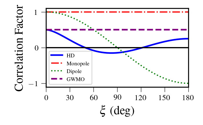
We can compute the OS for different correlations by using different ORFs. In addition to the HD and GWMO ORFs given in Eqs. (15) and (16), we also consider a standard dipole ORF and monopole ORF:
| (17) | |||||
| (18) |
In Figure 1, we plot all four ORFs used in this paper. Note that the monopole and GWMO are both constant as a function of angular separation, but the monopole as a value of while the GWMO as a value of . This means that any signal that fits one will also fit the other, but the inferred amplitudes will differ because the two ORFs have different normalizations.
We can measure the overlap between different ORFs by computing the “unweighted match statistic” Cornish and Sampson (2016),
| (19) |
where and are two different ORFs. This overlap depends on the number of pulsars in the PTA and their sky locations. Table 1 lists the match statistics for the four ORFs considered in this paper for our simulated PTA, which is based on the NANOGrav 12.5-year data set.
| GW-like | ||||
| Correlation | HD | Monopole | Dipole | monopole |
| HD | 1 | 0.255 | 0.435 | 0.255 |
| Monopole | 1 | 0.395 | 1 | |
| Dipole | 1 | 0.395 | ||
| GW-like | 1 | |||
| monopole |
IV Results
Here we present the results of analyzing our simulated data sets using the standard OS calculation and the modified MCOS. We show two types of simulations: one with an injected GWB (i.e., a common stochastic process with HD correlations), and one with both HD and GWMO correlations. We present the recovered OS values and corresponding signal-to-noise ratios (S/N) for different spatial correlations, and compare them to the injected values. We note the fraction of realizations with 3 in Appendix A.
We also look at how accurately the OS and MCOS recover the amplitude of the correlated process. If a non-negligible correlated signal is present in the data, then the expressions for and given in Eqs. (4), (5), (11), and (12) must be revised to include interpulsar pair correlation (Allen and Romano, 2023; Johnson et al., 2023). For more details, see App. C. We use the recovered and to compute the percentile of the injected value, assuming a Gaussian distribution111As shown in Hazboun et al. (2023), the optimal statistic actually follows a generalized chi-squared distribution and not a Gaussian distribution. In this work, we approximate the distribution as a Gaussian, owing to the computational expense of constructing the generalized chi-squared distribution for each simulation. This is a reasonably good approximation, and has been used in previous work (Vigeland et al., 2018; Johnson et al., 2023)., and compare the fraction of simulations for
Finally, we look at how much the data preferred models with multiple correlated signals using the Akaike Information Criterion (AIC) Akaike (1998), which is a frequentist analog for the Bayes factor. It is given by
| (20) |
where is the number of model parameters (i.e., the number of correlated signal amplitudes, or the number of ORFs), and the chi-squared given by Eq. (3) for a single correlated signal and Eq. (7) for multiple correlated signals The factor of acts as an Occam’s penalty for adding more parameters to a model. We compute using the maximum-likelihood red noise parameters. The relative probability of two models is then given by
| (21) |
where represents the minimum AIC value of all the different models. The model with the minimum AIC will thus be the most preferred model, with a p(AIC) = 1. Some of the models are equally preferred, with the difference in their AIC 0.01, so we set a threshold value of p(AIC) 0.99 to account for these cases. These results are also presented in Appendix A.
IV.1 HD simulation
We created 200 simulations with an injected HD
which we analyzed using the traditional OS and the MCOS. A complete summary of the results can be found in Table 2 in Appendix A. When we search for one spatial correlation at a time, we find a S/N for HD correlations in 17% of the simulations, but we also find S/N for monopole and dipole correlations in 6% and 5% of the simulations, respectively, even though there are no monopole-correlated or dipole-correlated signals present in the data sets. In Figure 2, we show histograms for the recovered distributions of and the S/N for HD, monopole, and dipole correlations. On average, we recover higher S/N of HD correlations than for monopole or dipole correlations; however, we recover S/N for monopole and dipole correlations in more than half of the simulations, as shown by the dotted lines in Fig. 2.
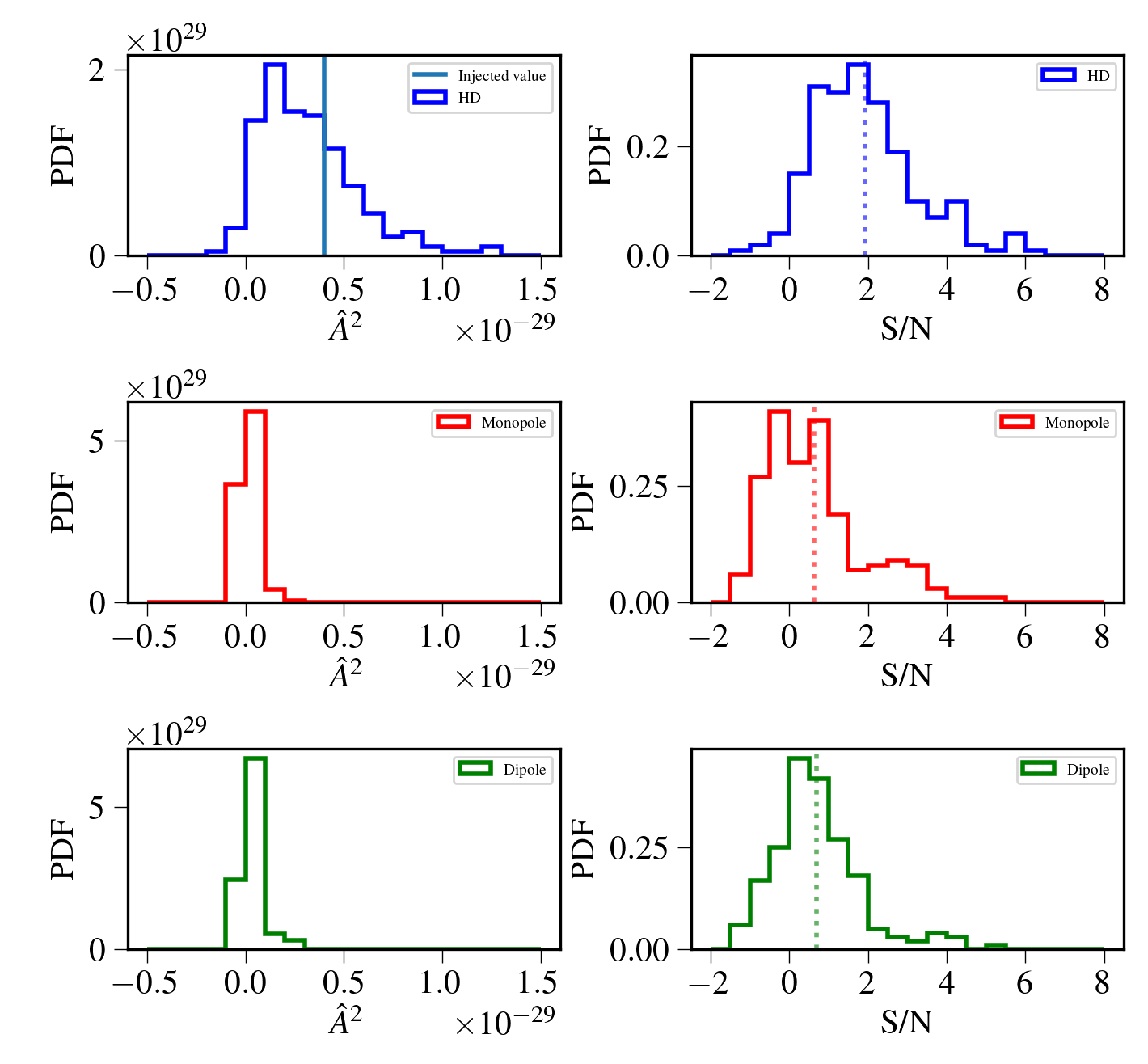
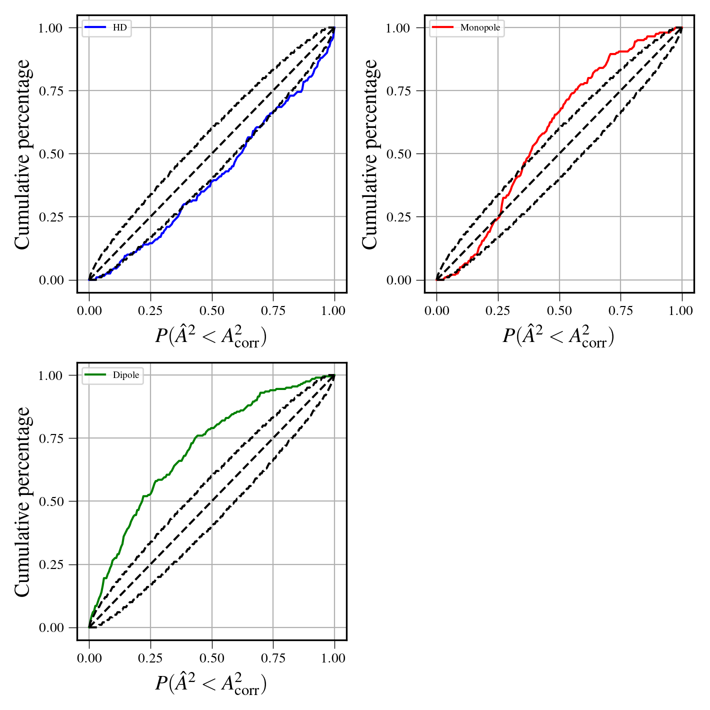
Figure 3 shows plots for the recovered single component OS using HD, monopole, and dipole correlations. For each simulation, we use the marginalized chain values to calculate and , taking pulsar pair cross covariance into consideration, and then compute the percentile of the injected value for that type of correlation.
We then plot the cumulative fraction of realizations for which the injected value is at that percentile. If the parameters are accurately recovered, we would expect the cumulative fraction of realizations to be equal to the cumulative percentile. If it is not, that indicates the parameter is being overestimated (over the central dashed black line) or underestimated (under the central dashed black line). We find that the amplitude of HD correlations is underestimated, while the amplitudes of monopole and dipole correlations (which were not injected) are overestimated. The underestimation of the amplitude of HD correlations is likely due to two factors: first, there is covariance between the pulsars’ intrinsic red noise and common red noise, and second, the simulations inject the intrinsic red noise and common red noise over more frequency components than we use to recover them.
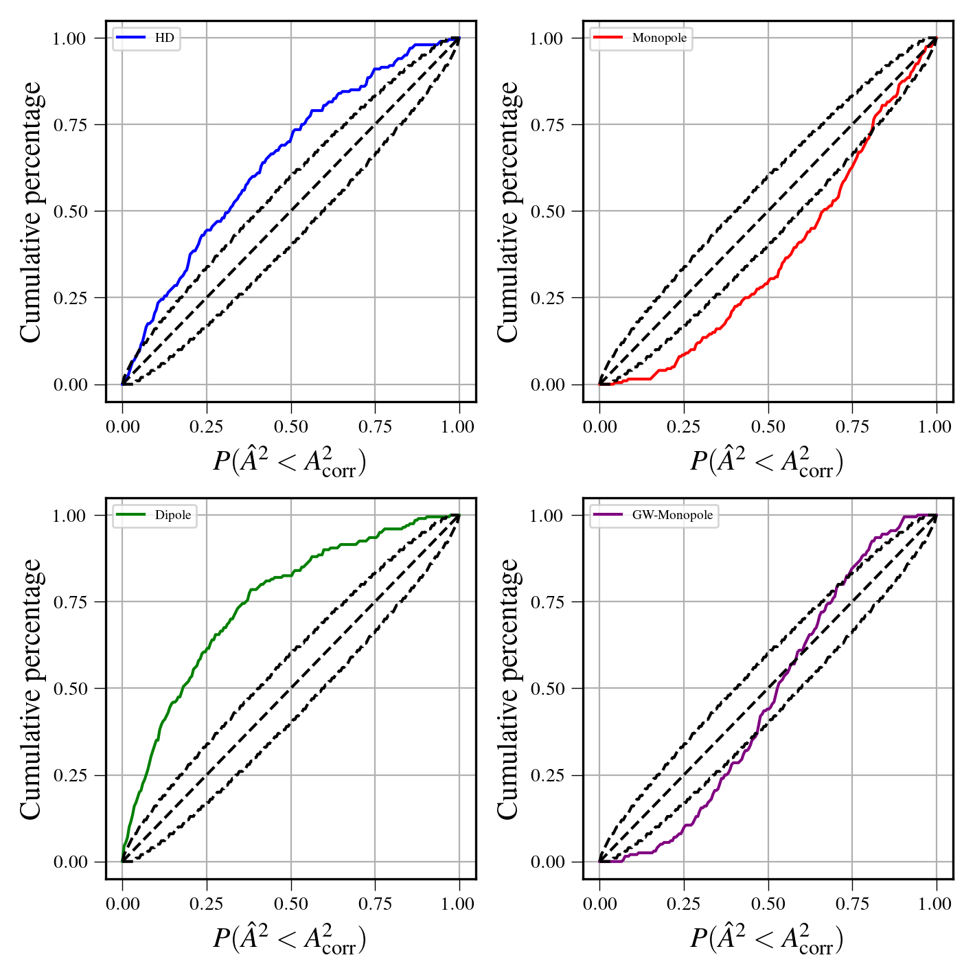
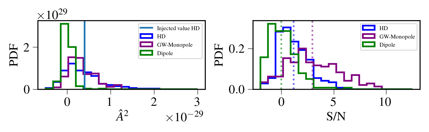
In contrast, the MCOS more accurately recovers the amplitude of monopole and dipole correlations. We show the recovered distributions of and the S/N for models consisting of multiple correlations in Figure 4. The distributions for the amplitude and S/N of HD correlations are similar to those obtained when fitting for only HD correlations (Figure 2, top row), but now the distributions for the amplitude and S/N of monopole and dipole correlations are centered around zero. The plots, shown in Figure 5, show the recovery of the MCOS . We find that MCOS analysis recovers the injected parameters for the monopole and dipole ORFs more accurately than the OS. The amplitude of HD correlations is slightly underestimated, as it was when using the OS.
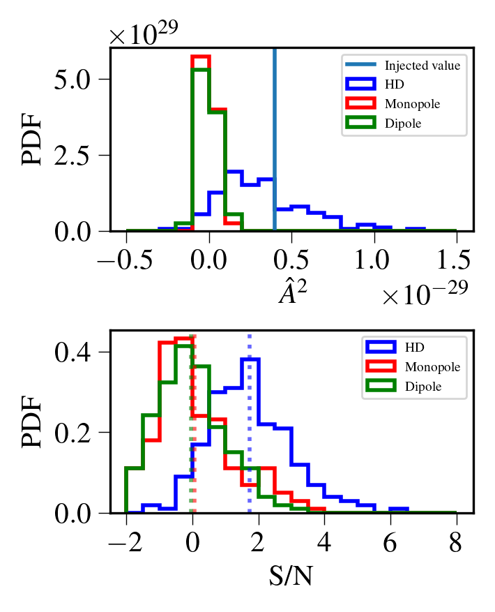
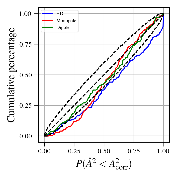
Table 2 lists the percentage of ORFs where an S/N greater than 3 was recovered, as well as the percentage of cases where the particular model had the lowest AIC value (most preferential model). In 51.5 % of realizations, the standard OS, HD ORF model had the lowest AIC value, as expected, considering our injection has only one signal present. The standard monopole and monopole+HD model have nearly the same preference. We note that these simulations include relatively low-significance HD correlations, as can be seen by the fact that the HD S/N in only 17% of simulations. ut the percentage of models with an HD S/N does not change drastically between the individual and MCOS models. This means that it is difficult to distinguish between different correlations. Nevertheless, the MCOS analysis allows us to search for the presence of spatial correlations and compute the relative probability of different models.
IV.2 HD + GWMO simulations
Finally, we looked at how well the MCOS could recover multiple correlated signals. We generated 200 simulations that contained two stochastic processes: one with HD correlations and one with GWMO correlations. We used the same amplitude and spectral index for both processes. We summarize the results of analyzing these simulations in Table 3 in Appendix A.
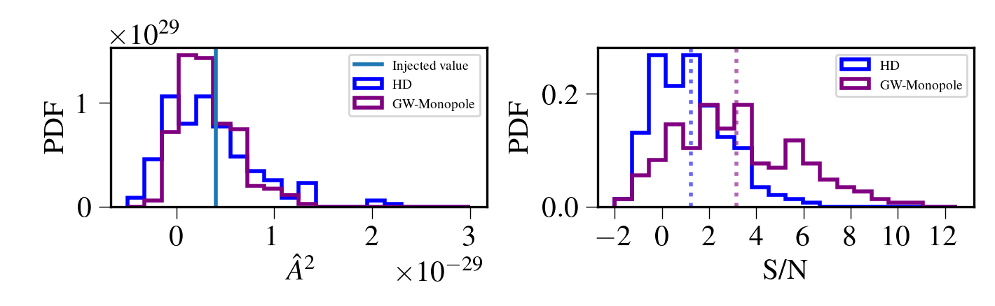
When we analyze the simulations for a single correlation, we find S/N for HD correlations in 27% of simulations and for GWMO in 56% of simulations. As shown in Figure 6, we recover the GWMO signal with higher mean S/N than the HD signal. We note that the correlation coefficient for HD correlations is less than the correlation coefficient for GWMO correlations for all angular separations (except for zero), which is why the OS recovers the GWMO signal with a higher S/N than the HD signal – even though the HD and GWMO signals have the same amplitude, the GWMO signal has significantly more power in the cross-correlations than the HD signal.
We also recover a dipole signal with S/N in 21% of simulations even though no such signal has been injected.
Figure 7 shows p-p plots for HD, monopole, dipole, and GWMO correlations. Since the data contain both HD and GWMO-correlated processes, but we are only fitting one process at a time, both signals are being incorrectly associated with a single correlation, resulting in inaccurate parameter estimation. When we fit to HD correlations only, this results in a significant overestimate of the HD-correlated amplitude. When we fit to GWMO correlations only, the amplitude estimate is not as affected, but the uncertainty is underestimated. We also see that the amplitude of a dipolar process is overestimated, even though one is not present.

When we use the MCOS, we find that we are able to more accurately recover the amplitudes of all the correlated processes. Figure 8 shows the recovered amplitudes and S/N, while Figure 9 shows p-p plots for the recovered amplitudes. When fitting for both HD and GWMO signals, the amplitudes are more accurately recovered than when fitting for only one signal at a time, although the amplitudes are slightly underestimated. This is possibly because of covariance between the pulsar noise and the common signals. We also find that when we include dipole correlations in our model, we accurately recover that no dipole signal is present, and the addition of the dipole signal does not affect the recovery of either the HD and GWMO signals.

V Conclusions
In this paper, we present a generalization of the OS that can simultaneously search for multiple correlated signals. As we have shown, this allows us to better distinguish between different spatial correlations. For a real PTA, the ORFs corresponding to different correlations are not orthogonal as shown in Table 1. The overlap between them can lead to non-zero S/N recovery of non-injected signals. It is also useful in cases where multiple correlated signals, e.g., a GWB and correlated noise, are present in the data. We have also performed model selection by computing the AIC, which acts as a pseudo-Bayes factor.
We have tested this method using two simulated data sets. The first contained a stochastic signal with HD correlations. When fitting only a single correlation, we found that we overestimated the presence of correlations that were not present, but using the MCOS eliminated this problem.
We also generated simulated data sets that contained both HD and GWMO-correlated signals. We demonstrated that the MCOS allows both signals to be recovered while ruling out any non-injected signals.
In this paper, we have considered four types of correlations: HD, monopole, dipole, and GWMO. This method can be used with any number and type of correlations. In the NANOGrav 15-year gravitational wave background search Agazie et al. (2023), the MCOS was used to search for evidence of monopolar or dipolar processes, which could be associated with correlated noise sources such as clock errors or ephemeris errors Roebber (2019); Vallisneri et al. (2020); Hobbs et al. (2020), and to do a model-independent reconstruction of the correlations using Legendre polynomials Gair et al. (2014). It was also used in the search of the NANOGrav 15-year data set for evidence of non-Einsteinian polarizations Agazie et al. (2023). The modular nature of the MCOS makes it a valuable tool for characterizing the nature of correlations in PTA data sets.
Acknowledgements.
We thank Justin Ellis, Jeff Hazboun, David Kaplan, Dusty Madison, Pat Meyers, Gabe Freedman, Joe Romano, Xavier Siemens, Abhimanyu Susobhanan, and Michele Vallisneri for useful discussions. We thank Nima Laal for help creating simulated data sets with monopole injections. This work was supported by National Science Foundation (NSF) grant PHY-2011772. SRT acknowledges support from NSF AST-2007993 and AST-2307719. SRT and KAG also acknowledge support from an NSF CAREER #2146016. The authors are members of the NANOGrav collaboration, which receives support from NSF Physics Frontiers Center award number 1430284 and 2020265.Appendix A Simulation results
This appendix contains the results of the MCOS analysis on the HD (Table 2), and HD+GWMO (Table 3) simulations. The middle three columns refer to the percentage of realizations where the ORF listed in the top row had a S/N greater than or equal to three. The last column shows the percentage of realizations where the particular model listed was the most favored, with a . Since certain realizations had AIC values very similar to one another, implying that more than one model was equally favored, we have set our p(AIC) threshold to 0.99.
| % of Simulations with S/N | % of Simulations | |||
| Model | HD | Monopole | Dipole | with |
| HD only | 17.5% | 40% | ||
| Monopole only | 7% | 18% | ||
| Dipole only | 5% | 14% | ||
| HD + monopole | 16.5% | 2% | 15.5% | |
| HD + dipole | 16% | 1% | 8.5% | |
| Monopole + dipole | 3% | 2% | 1% | |
| HD + monopole + dipole | 14.5% | 2% | 0.5% | 5% |
| % of Simulations with S/N | % of Simulations | ||||
| Model | HD | GWMO | DI | MO | with |
| HD | 27.5% | 13.5% | |||
| GWMO | 53.5% | 39% | |||
| Dipole | 21% | 7.5% | |||
| Monopole | 53.5% | 39% | |||
| HD+GWMO+Dipole | 10.5% | 44% | 2% | 18.5% | |
| HD+Monopole+Dipole | 10.5% | 2% | 44% | 18.5% | |
| HD+GWMO | 13.5% | 48% | 19.5% | ||
| HD+Monopole | 13.5% | 48% | 19.5% | ||
| HD+Dipole | 16.5% | 10% | 2.5% | ||
| GWMO+Dipole | 46.5% | 5% | 0% | ||
Appendix B Pulsar Red Noise Parameters
Our simulated data sets include intrinsic red noise in each pulsar. We model the red noise with a power-law power spectrum (as shown in Equation 14. The values of and used for each pulsar are listed in Table 4, and are based on the noise properties of the NANOGrav 12.5-year data set.
Pulsar injected injected B1855+09 -14.3053 5.5879 B1937+21 -13.4731 3.6189 B1953+29 -12.7813 1.1485 J0023+0923 -13.2146 0.2572 J0030+0451 -14.8837 5.1835 J0340+4130 -17.2031 0.3121 J06130200 -17.8287 6.9765 J0636+5128 -16.6117 0.4274 J0645+5158 -19.3925 6.2542 J0740+6620 -18.3882 0.8377 J09311902 -19.3076 3.1884 J1012+5307 -12.7970 0.9968 J10240719 -17.2779 2.5507 J1125+7819 -12.4459 1.5990 J1453+1902 -18.9550 4.9088 J14553330 -19.2175 6.2343 J16003053 -13.3480 0.0627 J16142230 -19.8669 2.5180 J1640+2224 -16.3220 5.6796 J16431224 -12.2480 1.1554 J1713+0747 -14.0354 0.3368 J1738+0333 -19.5594 5.2048 J1741+1351 -14.3474 1.9857 J17441134 -13.3903 1.5453 J17474036 -12.7570 3.5500 J18320836 -13.1021 1.6074 J1853+1303 -13.3632 1.3637 J1903+0327 -12.2570 1.8621 J19093744 -13.9843 1.7386 J1910+1256 -16.0932 2.6105 J1911+1347 -13.4836 1.7034 J19180642 -19.7173 4.0390 J1923+2515 -17.7267 1.7844 J1944+0907 -13.2678 1.2939 J20101323 -18.9887 0.8175 J2017+0603 -17.8317 1.9894 J2033+1734 -17.3183 3.8762 J2043+1711 -17.5979 2.8240 J21450750 -12.9290 1.2728 J2214+3000 -16.9390 4.6045 J2229+2643 -17.4349 6.1385 J2234+0611 -13.5827 3.6588 J2234+0944 -18.1712 0.7777 J2302+4442 -14.7765 2.8715 J2317+1439 -18.1829 6.5325
Appendix C Incorporating Pair Covariance into the OS and MCOS
In the weak-signal regime, our pulsar pair cross-correlations and their associated uncertainties as described in Equations 1 and 2, are given by Demorest et al. (2013); Pol et al. (2022); Chamberlin et al. (2015); Siemens et al. (2013); Vigeland et al. (2018)
| (22) | |||||
| (23) |
where is the auto-covariance matrix of pulsar , is the cross-covariance matrix between pulsars and , and . The auto-correlation matrices contain contributions from white noise, intrinsic red noise, and the common process red noise, while the cross-correlation matrices only considers contributions from the common process. The definition of the cross-correlation uncertainties in Equation 23 is only valid in the weak-signal regime and does not include correlations between different pairs of pulsars arising from the fact that some of the pulsar pairs will have pulsars in common (e.g., the correlations and both have the pulsar in common).
If a significant correlated signal is present, then is an underestimate of the cross-correlation uncertainties. When we consider the covariances between different pairs of pulsars, our uncertainties must include an extra term for inter-pulsar pair covariances. For two pulsar pairs and Johnson et al. (2023),
| (25) | |||||
Note that is dependent on the ORF and amplitude of the common process, due to the contributions from .
For the standard single component OS,
| (26) | |||||
where is the ORF for the correlation, and is the amplitude of the common uncorrelated red noise found from a Bayesian analysis. We chose to use the amplitude of the common uncorrelated red noise here instead of the amplitude of the correlated process because it .
When we include pair covariance, the expressions for the OS and its variance become
| (27) | |||||
| (28) |
For the MCOS, we generalize Eqs. (27) and (28) to allow for arrays of and :
| (29) |
where is the index of the ORF.
To obtain the amplitudes of the correlated signals , we first calculate the MCOS values neglecting pair covariance using Eq. (11).
If any of the values for are negative, we set it equal to zero. We then set to be equal to a weighted fraction of the common uncorrelated red noise amplitude,
| (30) |
Then the MCOS covariance matrix becomes
| (31) | |||||
then, as we did in Section II, we can replace the with our new covariance and construct our new MCOS and matrices
| (32) | |||||
| (33) | |||||
| (34) | |||||
| (35) |
References
- Sesana (2013) A. Sesana, Classical and Quantum Gravity 30, 244009 (2013), eprint 1307.4086.
- Sesana et al. (2004) A. Sesana, F. Haardt, P. Madau, and M. Volonteri, ApJ 611, 623 (2004), eprint astro-ph/0401543.
- Burke-Spolaor et al. (2019) S. Burke-Spolaor, S. R. Taylor, M. Charisi, T. Dolch, J. S. Hazboun, A. M. Holgado, L. Z. Kelley, T. J. W. Lazio, D. R. Madison, N. McMann, et al., A&A Rev. 27, 5 (2019), eprint 1811.08826.
- Sazhin (1978) M. V. Sazhin, Soviet Ast. 22, 36 (1978).
- Detweiler (1979) S. Detweiler, ApJ 234, 1100 (1979).
- Foster and Backer (1990) R. S. Foster and D. C. Backer, ApJ 361, 300 (1990).
- Ransom et al. (2019) S. Ransom, A. Brazier, S. Chatterjee, T. Cohen, J. M. Cordes, M. E. DeCesar, P. B. Demorest, J. S. Hazboun, M. T. Lam, R. S. Lynch, et al. (The NANOGrav Collaboration), in BAAS (2019), vol. 51, p. 195.
- Desvignes et al. (2016) G. Desvignes, R. N. Caballero, L. Lentati, J. P. W. Verbiest, D. J. Champion, B. W. Stappers, G. H. Janssen, P. Lazarus, S. Osłowski, S. Babak, et al., MNRAS 458, 3341 (2016), eprint 1602.08511.
- Reardon et al. (2016) D. J. Reardon, G. Hobbs, W. Coles, Y. Levin, M. J. Keith, M. Bailes, N. D. R. Bhat, S. Burke-Spolaor, S. Dai, M. Kerr, et al., MNRAS 455, 1751 (2016).
- Tarafdar et al. (2022) P. Tarafdar, K. Nobleson, P. Rana, J. Singha, M. A. Krishnakumar, B. C. Joshi, A. K. Paladi, N. Kolhe, N. D. Batra, N. Agarwal, et al., PASA 39, e053 (2022), eprint 2206.09289.
- Perera et al. (2019) B. B. P. Perera, M. E. DeCesar, P. B. Demorest, M. Kerr, L. Lentati, D. J. Nice, S. Osłowski, S. M. Ransom, M. J. Keith, Z. Arzoumanian, et al., MNRAS 490, 4666 (2019), eprint 1909.04534.
- Hellings and Downs (1983) R. W. Hellings and G. S. Downs, ApJ 265, L39 (1983).
- Hobbs et al. (2012) G. Hobbs, W. Coles, R. N. Manchester, M. J. Keith, R. M. Shannon, D. Chen, M. Bailes, N. D. R. Bhat, S. Burke-Spolaor, D. Champion, et al., MNRAS 427, 2780 (2012), eprint 1208.3560.
- Tiburzi et al. (2016) C. Tiburzi, G. Hobbs, M. Kerr, W. A. Coles, S. Dai, R. N. Manchester, A. Possenti, R. M. Shannon, and X. P. You, MNRAS 455, 4339 (2016), eprint 1510.02363.
- Hobbs et al. (2020) G. Hobbs, L. Guo, R. N. Caballero, W. Coles, K. J. Lee, R. N. Manchester, D. J. Reardon, D. Matsakis, M. L. Tong, Z. Arzoumanian, et al., MNRAS 491, 5951 (2020), eprint 1910.13628.
- Lee et al. (2008) K. J. Lee, F. A. Jenet, and R. H. Price, The Astrophysical Journal 685, 1304 (2008), URL https://dx.doi.org/10.1086/591080.
- Chamberlin and Siemens (2012) S. J. Chamberlin and X. Siemens, Phys. Rev. D 85, 082001 (2012), eprint 1111.5661.
- Gair et al. (2015) J. R. Gair, J. D. Romano, and S. R. Taylor, Physical Review D 92 (2015), URL https://doi.org/10.1103%2Fphysrevd.92.102003.
- Cornish et al. (2018) N. J. Cornish, L. O’Beirne, S. R. Taylor, and N. Yunes, Physical Review Letters 120 (2018), URL https://doi.org/10.1103%2Fphysrevlett.120.181101.
- Anholm et al. (2009) M. Anholm, S. Ballmer, J. D. E. Creighton, L. R. Price, and X. Siemens, Phys. Rev. D 79, 084030 (2009), eprint 0809.0701.
- Demorest et al. (2013) P. B. Demorest, R. D. Ferdman, M. E. Gonzalez, D. Nice, S. Ransom, I. H. Stairs, Z. Arzoumanian, A. Brazier, S. Burke-Spolaor, S. J. Chamberlin, et al., ApJ 762, 94 (2013), eprint 1201.6641.
- Chamberlin et al. (2015) S. J. Chamberlin, J. D. E. Creighton, X. Siemens, P. Demorest, J. Ellis, L. R. Price, and J. D. Romano, Phys. Rev. D 91, 044048 (2015), eprint 1410.8256.
- Vigeland et al. (2018) S. J. Vigeland, K. Islo, S. R. Taylor, and J. A. Ellis, Phys. Rev. D 98, 044003 (2018), eprint 1805.12188.
- Arzoumanian et al. (2021) Z. Arzoumanian, P. T. Baker, H. Blumer, B. Bécsy, A. Brazier, P. R. Brook, S. Burke-Spolaor, M. Charisi, S. Chatterjee, S. Chen, et al., ApJ 923, L22 (2021), eprint 2109.14706.
- Alam et al. (2021) M. F. Alam, Z. Arzoumanian, P. T. Baker, H. Blumer, K. E. Bohler, A. Brazier, P. R. Brook, S. Burke-Spolaor, K. Caballero, R. S. Camuccio, et al., ApJS 252, 4 (2021), eprint 2005.06490.
- Arzoumanian et al. (2020) Z. Arzoumanian, P. T. Baker, H. Blumer, B. Bécsy, A. Brazier, P. R. Brook, S. Burke-Spolaor, S. Chatterjee, S. Chen, J. M. Cordes, et al., ApJ 905, L34 (2020), eprint 2009.04496.
- Phinney (2001) E. S. Phinney, arXiv e-prints astro-ph/0108028 (2001), eprint astro-ph/0108028.
- Jenet and Romano (2015) F. A. Jenet and J. D. Romano, American Journal of Physics 83, 635 (2015), eprint 1412.1142.
- Vallisneri (2020) M. Vallisneri, Astrophysics Source Code Library p. ascl:2002.017 (2020), URL https://ui.adsabs.harvard.edu/abs/2020ascl.soft02017V.
- Ellis et al. (2020) J. A. Ellis, M. Vallisneri, S. R. Taylor, and P. T. Baker, ENTERPRISE: Enhanced Numerical Toolbox Enabling a Robust PulsaR Inference SuitE, Zenodo (2020).
- Taylor et al. (2021) S. R. Taylor, P. T. Baker, J. S. Hazboun, J. Simon, and S. J. Vigeland, enterprise_extensions (2021), v2.3.3, URL https://github.com/nanograv/enterprise_extensions.
- Ellis and van Haasteren (2019) J. Ellis and R. van Haasteren, PTMCMCSampler: Parallel tempering MCMC sampler package written in Python, Astrophysics Source Code Library, record ascl:1912.017 (2019), eprint 1912.017.
- Cornish and Sampson (2016) N. J. Cornish and L. Sampson, Phys. Rev. D 93, 104047 (2016), eprint 1512.06829.
- Allen and Romano (2023) B. Allen and J. D. Romano, Phys. Rev. D 108, 043026 (2023), URL https://link.aps.org/doi/10.1103/PhysRevD.108.043026.
- Johnson et al. (2023) A. D. Johnson, P. M. Meyers, P. T. Baker, N. J. Cornish, J. S. Hazboun, T. B. Littenberg, J. D. Romano, S. R. Taylor, M. Vallisneri, S. J. Vigeland, et al., arXiv e-prints arXiv:2306.16223 (2023), eprint 2306.16223.
- Hazboun et al. (2023) J. S. Hazboun, P. M. Meyers, J. D. Romano, X. Siemens, and A. M. Archibald (2023), eprint 2305.01116.
- Akaike (1998) H. Akaike, Information Theory and an Extension of the Maximum Likelihood Principle (Springer New York, New York, NY, 1998), pp. 199–213, ISBN 978-1-4612-1694-0, URL https://doi.org/10.1007/978-1-4612-1694-0_15.
- Agazie et al. (2023) G. Agazie, A. Anumarlapudi, A. M. Archibald, Z. Arzoumanian, P. T. Baker, B. Bécsy, L. Blecha, A. Brazier, P. R. Brook, S. Burke-Spolaor, et al., ApJ 956, L3 (2023), eprint 2306.16221.
- Roebber (2019) E. Roebber, ApJ 876, 55 (2019), eprint 1901.05468.
- Vallisneri et al. (2020) M. Vallisneri, S. R. Taylor, J. Simon, W. M. Folkner, R. S. Park, C. Cutler, J. A. Ellis, T. J. W. Lazio, S. J. Vigeland, K. Aggarwal, et al., ApJ 893, 112 (2020), eprint 2001.00595.
- Gair et al. (2014) J. Gair, J. D. Romano, S. Taylor, and C. M. F. Mingarelli, Phys. Rev. D 90, 082001 (2014), URL https://link.aps.org/doi/10.1103/PhysRevD.90.082001.
- Agazie et al. (2023) G. Agazie et al. (NANOGrav) (2023), eprint 2310.12138.
- Pol et al. (2022) N. Pol, S. R. Taylor, and J. D. Romano, ApJ 940, 173 (2022), eprint 2206.09936.
- Siemens et al. (2013) X. Siemens, J. Ellis, F. Jenet, and J. D. Romano, Classical and Quantum Gravity 30, 224015 (2013), eprint 1305.3196.