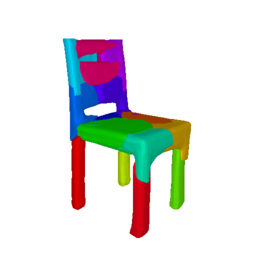
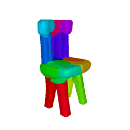
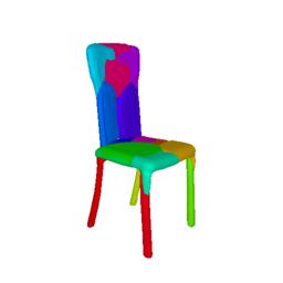
PartNeRF: Generating Part-Aware Editable 3D Shapes without 3D Supervision

Abstract

Impressive progress in generative models and implicit representations gave rise to methods that can generate 3D shapes of high quality. However, being able to locally control and edit shapes is another essential property that can unlock several content creation applications. Local control can be achieved with part-aware models, but existing methods require 3D supervision and cannot produce textures. In this work, we devise PartNeRF, a novel part-aware generative model for editable 3D shape synthesis that does not require any explicit 3D supervision. Our model generates objects as a set of locally defined NeRFs, augmented with an affine transformation. This enables several editing operations such as applying transformations on parts, mixing parts from different objects etc. To ensure distinct, manipulable parts we enforce a hard assignment of rays to parts that makes sure that the color of each ray is only determined by a single NeRF. As a result, altering one part does not affect the appearance of the others. Evaluations on various ShapeNet categories demonstrate the ability of our model to generate editable 3D objects of improved fidelity, compared to previous part-based generative approaches that require 3D supervision or models relying on NeRFs.

Abstract

In this supplementary document, we first present a detailed overview of our network architecture, the training and generation procedure, in Sec. A. We then provide ablations on how different components of our pipeline impact the performance of our model, in Sec. B. Subsequently, in Sec. C we provide additional results both on the shape generation task as well as on the shape editing task. Next, we demonstrate various applications of our model such as shape and image inversion, in Sec. D and Sec. E, respectively. Finally, in Sec. G, we analyse the limitations, future research directions and in Sec. H we discuss potential negative impact of our method on society.

1 Introduction

Generating realistic and editable 3D content is a long-standing problem in computer vision and graphics that has recently gained more attention due to the increased demand for 3D objects in AR/VR, robotics and gaming applications. However, manual creation of 3D models is a laborious endeavor that requires technical skills from highly experienced artists and product designers. On the other hand, editing 3D shapes, typically involves re-purposing existing 3D models, by manually changing faces and vertices of a mesh and modifying its respective UV-map [104]. To accommodate this process, several recent works introduced generative models that go beyond generation and allow editing the generated instances [129, 69, 128, 62, 20, 85, 111, 14, 137, 59]. Shape editing involves making local changes on the shape and the appearance of different parts of an object. Therefore, having a basic understanding of the decomposition of the object into parts facilitates controlling what to edit.

While Generative Adversarial Networks (GANs) [33] have emerged as a powerful tool for synthesizing photorealistic images [8, 16, 17, 52, 54, 53], scaling them to 3D data is non-trivial as they ignore the physics of image formation process along a viewing direction. To address this, 3D-aware GANs incorporate 3D representations such as voxel grids [42, 80, 83] in generative settings or combine them with differentiable renderers [64, 139]. While they faithfully recover the geometry and appearance, they do not allow changing specific parts of the object.

Inspired by the rapid evolution of neural implicit rendering techniques [76], recent works [105, 85, 126, 9, 35] proposed to combine them with GANs in order to allow for multi-view-consistent generations of high quality. Despite their impressive performance on novel view synthesis, their editing capabilities are limited. To this end, editing operations in the latent space have been explored [23, 69, 47, 127, 137] but these approaches lack intuitive control over the shape. By decomposing shapes into parts, other works facilitate structure-aware shape manipulations [78, 123, 44, 97]. However, they require 3D supervision during training and can only operate on textureless shapes.

To address these limitations, we devise PartNeRF, a novel part-aware generative model, implemented as an auto-decoder [6]. Our model enables part-level control, which facilitates various editing operations on the shape and appearance of the generated instance. These operations include rigid and non-rigid transformations on the object parts, part mixing from different objects, removing/adding parts and editing the appearance of specific parts of the object.

Our key idea is to represent the objects using a set of locally defined Neural Radiance Fields (NeRFs) that are arranged such that the object can be plausibly rendered from a novel view. To enable part-level control, we enforce a hard assignment between parts and rays that ensures that altering one part does not affect the shape and appearance of other parts. Our model does not require any explicit 3D supervision; we only assume supervision from images and object masks captured from known cameras. We evaluate PartNeRF on various ShapeNet categories and demonstrate that it can generate textured shapes of higher fidelity than methods that assume 3D supervision as well as approaches that rely on NeRFs. Furthermore, we showcase various editing operations that were not previously possible.

In summary, we make the following contributions: We propose the first part-aware generative model that parametrizes parts as NeRFs. Among the existing generative pipelines that consider the decomposition of objects into parts, our work is the first that does not require explicit 3D supervision and enables editing operations both on the shape and the texture of the generated object. Code and data is available at https://ktertikas.github.io/part˙nerf.

2 Related Work

We now discuss the most relevant literature on 3D generative models in the context of generating editable shapes.

Neural Implicit Representations: Neural Implicit Representations [74, 91, 13] have demonstrated impressive capabilities on various tasks ranging from 3D reconstruction with [90, 102, 103, 89] and without texture [74, 91, 13, 75, 3, 125, 96, 4, 15, 48, 34, 101] to video encoding [12], 3D-aware generative modelling [105, 10, 85, 73, 22, 35, 9], inverse graphics [86, 132] and novel view synthesis [76, 136, 43, 120, 100]. In contrast to explicit representations i.e. point clouds, meshes and voxels, implicit representations encode the shape’s geometry and appearance in the weights of a neural network. Among the most extensively used implicit-based models are NeRFs [76], which combine an implicit neural network with volumetric rendering [50] to perform novel view synthesis. Due to their compelling results, numerous works have been introduced to improve the training and rendering time [68, 138, 98, 66, 113, 29, 99, 135, 79], the underlying geometry [90, 119], to better handle lighting variations [72, 5, 109, 7] and to encode shape priors for better generalization [136, 43, 115] and generation [105, 10]. For a thorough overview on NeRF-based approaches we refer readers to [114, 124]. In our work, we introduce a generative model for editable 3D shapes with texture. Specifically, we parametrize objects as a structured set of local NeRFs that are trained from posed images and object masks.

Figure 2: Method Overview. Our generative model is implemented as an auto-decoder and it comprises three main components: The Decomposition Network takes two object specific learnable embeddings $\{\mathbf{z}_{s},\mathbf{z}_{t}\}$ that represent its shape and texture and maps them to a set of $M$ latent codes that control the shape and texture of each part. First, we map $\mathbf{z}^{s}$ and $\mathbf{z}^{t}$ to $M$ per-part embeddings $\{\hat{\mathbf{z}}_{m}^{s}\}_{m=1}^{M}$ and $\{\hat{\mathbf{z}}_{m}^{t}\}_{m=1}^{M}$ using $M$ linear projections, which are then fed to two transformer encoders: $\tau^{s}_{\theta}$ and $\tau^{t}_{\theta}$, that predict the final per-part shape and texture embeddings, $\{\mathbf{z}_{m}^{s}\}_{m=1}^{M}$ and $\{\mathbf{z}_{m}^{t}\}_{m=1}^{M}$. Next, the Structure Network maps the per-part shape feature representation $\mathbf{z}_{m}^{s}$ to a rotation matrix $\mathbf{R}_{m}$, a translation vector $\mathbf{t}_{m}$ and a scale vector $\mathbf{s}_{m}$ that define the coordinate system of the m-th part and its spatial extent. The last component of our model is the Neural Rendering module that takes the 3D points along each ray, transformed to the coordinate frame of its associated part, and maps them to an occupancy and a color value. We use plate notation to denote repetition over the $M$ parts.

3D-Aware Image Generation: Incorporating 3D representations in generative settings [25, 40, 42, 41, 71, 81, 82, 35, 22, 38, 73, 84, 140] has significantly improved the quality of the generated images and increased control over various aspects of the image formation process. Likewise, radiance fields have been combined with GANs to allow for photorealistic image synthesis of objects [105, 10] and scenes [85]. More recently, [9] introduced a triplane-based architecture that leverages both implicit and explicit representations and can generate high resolution images. Concurrently, [27] combined differentiable surface modelling [26] with a differentiable renderer to generate high-quality textured meshes. Unlike [105, 10, 9, 27] that are part agnostic, our model generates objects with part-level control, hence unlocking editing operations not previously possible. Our formulation is closely related to the compositional representation of [85] but has two important differences. First, we enforce a hard assignment between rays and parts ensuring that the color of each part is only determined by one NeRF, thus enabling local editing. Moreover, we model the shape and texture of each part separately, hence enabling even more control.

Shape Editing using NeRFs: Our work falls into the category of implicit-based shape editing approaches that directly operate on the radiance field [69, 137, 127]. Recent methods [137, 127] extract meshes from a pre-trained NeRF and rely on deformation techniques [108, 49, 24, 67] to guide the rendering process. Unlike our approach, these models are scene specific and cannot capture shape and texture variations across an object class. An alternative line of research explored using separate embeddings for capturing the shape and texture variations of 3D shapes [69, 47]. They demonstrated various editing operations such as color modifications or removal of certain parts of the shape. However, as they do not consider parts, they rely on heuristics for controlling what needs to be changed. Instead, by incorporating parts, our model provides more intuitive control, when editing a 3D shape. Also similar to our work, [88] uses multi-view videos and decomposes the object using a set of ellipsoids. However, this model is scene-specific and cannot generate novel shapes. In the context of face editing [51, 112, 110], different models require video sequences and partial semantic masks [51], or posed images along with full semantic masks [112, 110]. In contrast, our work only requires posed images and 2D object masks at training.

Primitive-based Representations: Shape abstraction techniques represent 3D shapes using semantically consistent primitive arrangements across different instances in a class. This most often requires 3D supervision [28, 60, 61, 63, 87, 77, 106, 141, 19, 21, 32, 55, 93, 94, 116], although [130, 131] demonstrate that is possible to learn only from images. Unlike our parts, geometric primitives are typically simple shapes such as cuboids [116], spheres [37] or superquadrics [93, 94]. Due to their simple shape parametrization these primitives cannot capture complex geometries. To address this, recent works propose to increase the number of primitives [19, 55] or represent shapes using a family of homeomorphic mappings [92], or a structured set of implicit functions [30]. Similar to [92] our parts can capture complex geometries, but as we parametrize them with locally defined NeRFs, we do not require explicit 3D supervision.

Part-based Shape Editing: Part-based generative models [37, 123, 62, 44, 97] can generate plausible 3D shapes [77, 78, 129] and perform various editing operations such as part mixing [134, 65, 97] and shape manipulation [37, 44]. Closely related to our work are [37, 44] which employ primitives, such as spheres [37] and 3D Gaussians [45], to enable shape editing by explicitly [37] or implicitly [44] transforming them. However, both require 3D supervision and can only alter attributes related to the shape of the object.

3 Method

Our goal is to design a 3D part-aware generative model that can be trained without explicit 3D supervision. Moreover, we want our generated shapes to be editable, namely to be able to make local changes on the shape and texture of specific parts of the object. To this end, we represent objects using $M$ locally defined parts that are parametrized with a NeRF [76]. Defining NeRFs locally, i.e. in their own coordinate system, enables direct part-level control simply by applying transformations on the per-part coordinate system.

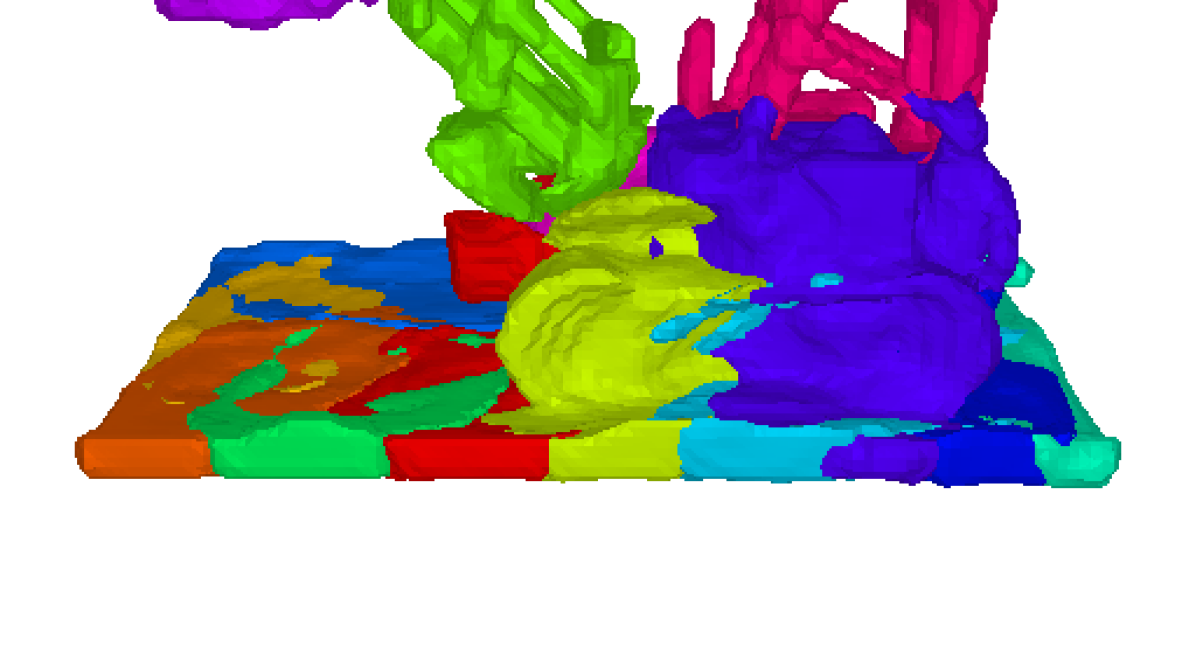
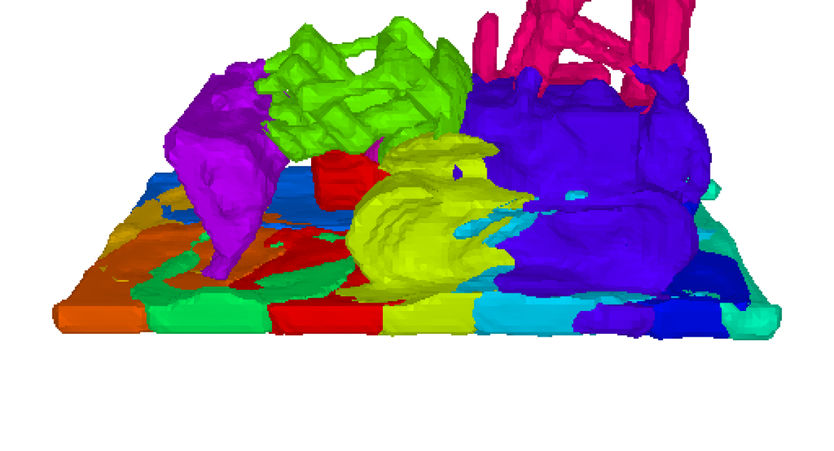
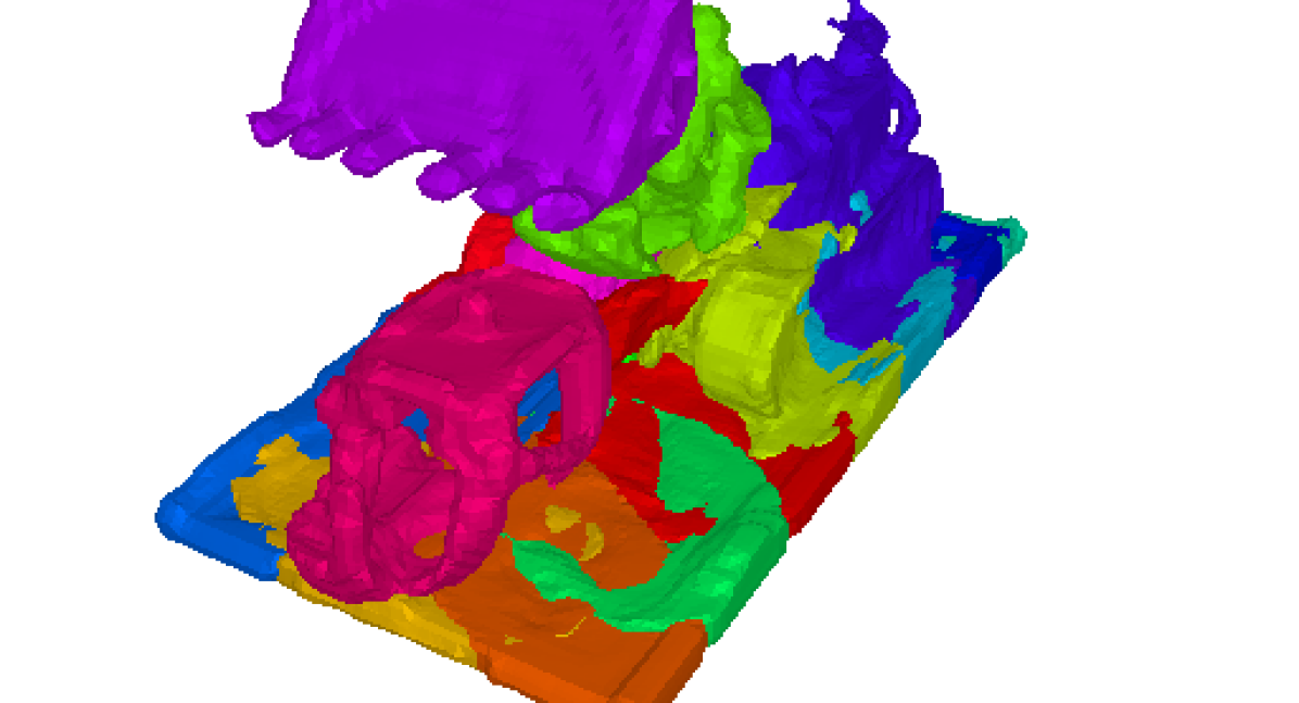
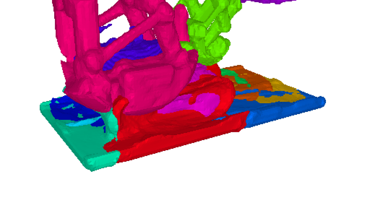
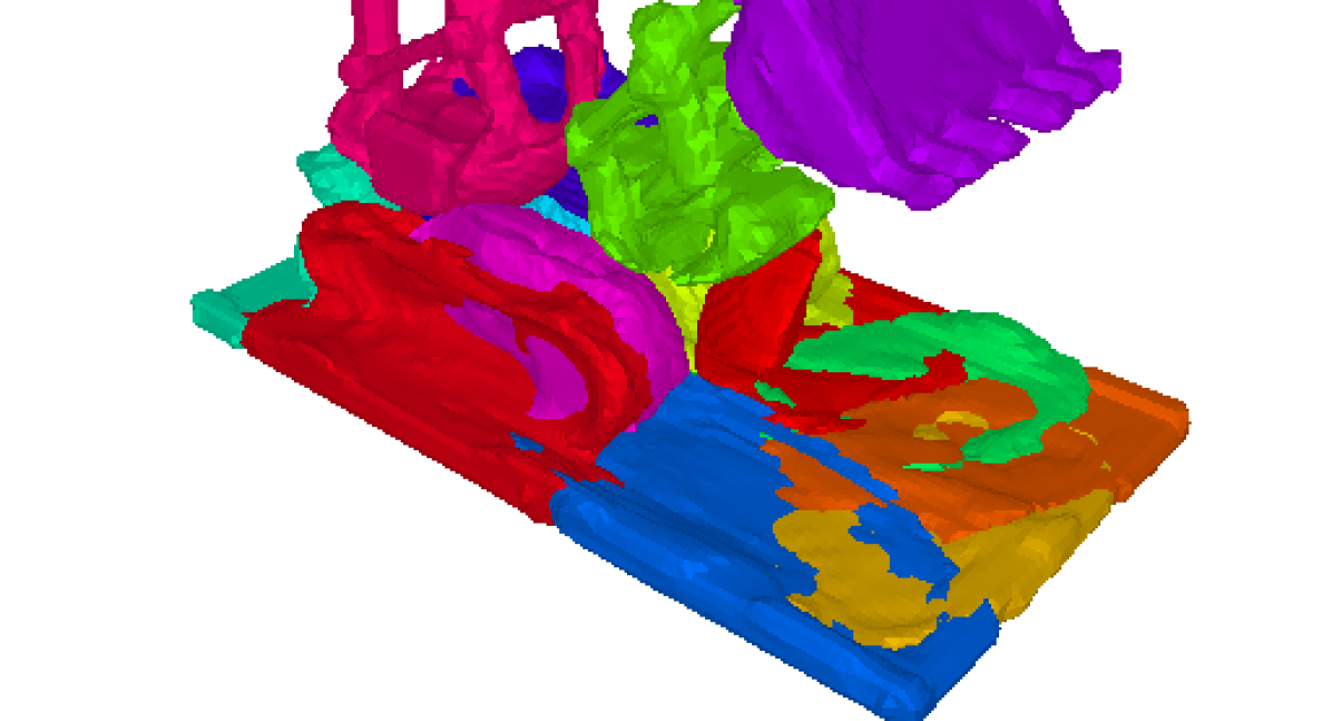
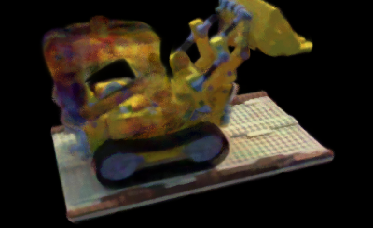
However, to achieve distinct, manipulable parts, it is essential that each object part is represented by a single NeRF. To enforce this, we introduce a hard assignment between rays and parts by associating a ray with the first part it intersects (Fig. 3). Namely, the color of each ray is predicted from a single NeRF, thus preventing combinations of parts reasoning about the color of a ray. Note that our formulation differs from [85], as we explicitly associate rays with parts, instead of simply combining them. This ensures that when editing one part, the shape and appearance of the others does not change (Fig. 1).

3.1 Neural Radiance Fields

Given a set of posed images of objects in a semantic class, each accompanied by an object mask, which is simply a binary image indicating whether each pixel is inside the object or not, we define $\mathcal{R}$, the complete set of rays from all views. For each ray $r=\{\mathbf{x}_{0}^{r}+t\mathbf{d}^{r}:t\geq 0\}$ with origin $\mathbf{x}_{0}^{r}$ and viewing direction $\mathbf{d}^{r}$, we denote $C(r)\in\mathbb{R}^{3}$ and $I(r)\in\{0,1\}$ the color value of the RGB image and the binary value of the mask, respectively, at the corresponding pixel. Finally, we sample a set of $N$ points $\mathcal{X}_{r}=\{\mathbf{x}_{1}^{r},\dots,\mathbf{x}_{N}^{r}\}$ along $r$, which are ordered by increasing distance from the origin $\mathbf{x}_{0}^{r}$, used for estimating the color along this ray using numerical quadrature [118].

Neural Radiance Fields: NeRFs [76] represent a scene as a continuous function, parametrized with an MLP, that maps a 3D point $\mathbf{x}\in\mathbb{R}^{3}$ and a viewing direction $\mathbf{d}\in\mathbb{S}^{2}$ into a color $\mathbf{c}\in\mathbb{R}^{3}$ and a volume density $\sigma\in\mathbb{R}^{+}$. Before passing the inputs $\mathbf{x}$ and $\mathbf{d}$ to the MLP, they are projected to a higher dimensional space by applying a fixed positional encoding [117] to each one of their elements. Given the predicted color and densities $\{\mathbf{c}_{i}^{r},\sigma_{i}^{r}\}_{i=1}^{N}$ for the $N$ sampled points $\mathcal{X}_{r}$ along ray $r$, its rendered color can be derived from

$$\hat{C}(r)=\sum_{i=1}^{N}\exp\Big{(}-\sum_{j<i}\sigma_{j}^{r}\delta_{j}^{r}\Big{)}(1-\exp(-\sigma_{i}^{r}\delta_{i}^{r}))\mathbf{c}_{i}^{r},$$ (1)

where $\delta_{i}^{r}$ is the distance between two adjacent samples along $r$. At training, the MLP is optimized by minimizing the error between observed and rendered images.

Alternatively, [90] propose predicting occupancies instead of densities, hence their rendering equation becomes

$$\hat{C}(r)=\sum_{i=1}^{N}o_{i}^{r}\prod_{j<i}\left(1-o_{j}^{r}\right)\mathbf{c}_{i}^{r},$$ (2)

where $o_{i}^{r}=1-\exp(-\sigma_{i}^{r}\delta_{i}^{r})$ is the occupancy value at point $\mathbf{x}_{i}^{r}$ and $\mathbf{c}_{i}^{r}$ its color. Similar to [90] we also predict occupancy values, as this facilitates associating rays with parts, hence enabling part-level control, as discussed in Sec. 3.2.

3.2 Parts as Neural Radiance Fields

We represent a 3D object using $M$ parts, where each part is parametrized as a NeRF. Note that we assume a fixed number of parts across all objects, namely the generated objects cannot have a variable number of parts. To learn the latent space of each NeRF, we follow [69] and condition it on two part-specific learnable latent codes: one for the shape and one for the texture, $\mathbf{z}_{m}^{s},\mathbf{z}_{m}^{t}$. These codes are obtained from a per-object specific learnable embedding (see Sec. 3.3). Disentangling the shape from the texture allows modifying one property without affecting the other.

Moreover, as we are interested in editing specific parts of the object, we want to be able to modify the pose, size, and appearance of each part independently. This can be enforced by making sure that each NeRF receives geometric inputs in its own local coordinate system. To this end, we augment each part with: (i) an affine transformation $\mathcal{T}_{m}(\mathbf{x})=\mathbf{R}_{m}(\mathbf{x}+\mathbf{t}_{m})$ that maps a 3D point $\mathbf{x}$ to the local coordinate system of the $m$-th part, where $\mathbf{t}_{m}\in\mathbb{R}^{3}$ is the translation vector and $\mathbf{R}_{m}\in SO(3)$ is the rotation matrix and (ii) a scale vector $\mathbf{s}_{m}\in\mathbb{R}^{3}$, representing its spatial extent. All are obtained from the per-part shape code $\mathbf{z}_{m}^{s}$.

Part Representation: Each part is represented as a continuous function that maps a 3D point $\mathbf{x}\in\mathbb{R}^{3}$, a viewing direction $\mathbf{d}\in\mathbb{S}^{2}$, a shape code $\mathbf{z}^{s}\in\mathbb{R}^{L_{s}}$ and a texture code $\mathbf{z}^{t}\in\mathbb{R}^{L_{t}}$ into a color $\mathbf{c}\in\mathbb{R}^{3}$ and an occupancy value $o\in[0,1]$. Similar to [90], we employ two separate networks: a color network $c_{\theta}$ and an occupancy network $o_{\theta}$ to predict the color and the occupancy value. Note that the occupancy value $o$ is constrained to $[0,1]$ with a sigmoid. More formally, each NeRF maps a 3D point $\mathbf{x}$ along a viewing direction $\mathbf{d}$ to a color $\mathbf{c}$ and an occupancy $o$ as:

$$c_{\theta}^{m}(\mathbf{x},\mathbf{d}) =c_{\theta}(\mathcal{T}_{m}(\mathbf{x}),\mathbf{R}_{m}\mathbf{d},\mathbf{z}_{m}^{s},\mathbf{z}_{m}^{t})$$ (3)

$$o_{\theta}^{m}(\mathbf{x}) =o_{\theta}(\mathcal{T}_{m}(\mathbf{x}),\mathbf{z}_{m}^{s}).$$ (4)

Note that while we apply positional encoding on the inputs, we omit it from (3)$+$(4) to avoid notation clutter.

To enforce that each part only captures continuous regions of the object, we multiply its occupancy function with the occupancy function of an axis-aligned 3D ellipsoid centered at the origin of the coordinate system, with axis lengths given by the scale vector $\mathbf{s}_{m}$. This results in the following joint occupancy function for the $m$-th part

$$h_{\theta}^{m}(\mathbf{x})=o_{\theta}^{m}(\mathbf{x})g_{\theta}^{m}(\mathbf{x}),$$ (5)

where $g_{\theta}^{m}(\mathbf{x})=g(T_{m}(\mathbf{x}),\mathbf{s}_{m})$ denotes the occupancy function of the $m$-th ellipsoid that is simply

$$g(\mathbf{x},\mathbf{s})=\sigma\left(\beta\left(1-\left\|{\operatorname{diag}(\mathbf{s})^{-1}\mathbf{x}}\right\|^{2}\right)\right),$$ (6)

where $\sigma(\cdot)$ is the sigmoid function and $\beta$ controls the sharpness of the transition. To estimate $g_{\theta}^{m}(\mathbf{x})$, we first transform $\mathbf{x}$ to the coordinate frame of the $m$-th part. This ensures that any transformation of the part, also transforms its ellipsoid.

Figure 3: Ray-Part Association. We illustrate the hard assignment between rays and parts in a 2D example with 3 parts and two rays $r$ and $r^{\prime}$. Since the association between rays and parts is determined based on the first part that a ray interests, the associations that emerge from (9) are $\mathcal{R}_{1}=\{r\},\mathcal{R}_{2}=\{\emptyset\}$ and $\mathcal{R}_{3}=\{r^{\prime}\}$.

Part Rendering: The rendering equation of the $m$-th part, given a set of $N$ sampled points along ray $r$ now becomes

$$\hat{C}_{m}(r)=\sum_{i=1}^{N}h_{\theta}^{m}(\mathbf{x}_{i}^{r})\prod_{j<i}\left(1-h_{\theta}^{m}(\mathbf{x}_{i}^{r})\right)c_{\theta}^{m}(\mathbf{x}_{i}^{r},\mathbf{d}^{r}).$$ (7)

Object Rendering: To ensure distinct, manipulable parts, we introduce a hard assignment between rays and parts, by associating a ray with the first part it intersects. Given the ordered set of points $\mathcal{X}_{r}$ sampled along ray $r$, we define the index of the first point inside the part that $r$ intersects as

$$\psi_{r}(m)=\min\left\{i\in\{1,\dots,N\}\,:\,h_{\theta}^{m}(\mathbf{x}_{i}^{r})\geq\tau\right\},$$ (8)

where $\tau$ is a threshold used to determine whether a point is inside the $m$-th part or not. This is illustrated in Fig. 3. We can now define the set of rays $\mathcal{R}_{m}$ associated with the $m$-th part, as the set of rays that first intersect with it, namely:

$$\mathcal{R}_{m}=\Bigl{\{}r\in\mathcal{R}\,:\,m=\operatorname*{argmin~{}}_{k\in\{0\dots M\}}\psi_{r}(k)\Bigr{\}}.\vspace{-0.5em}$$ (9)

Using the assignment of rays to parts and the per-part rendering equation (7), we can formulate the rendering equation for the entire object, using $M$ NeRFs as follows

$$\hat{C}(r)=\sum_{m=1}^{M}\mathbbm{1}_{r\in\mathcal{R}_{m}}\hat{C}_{m}(r).$$ (10)

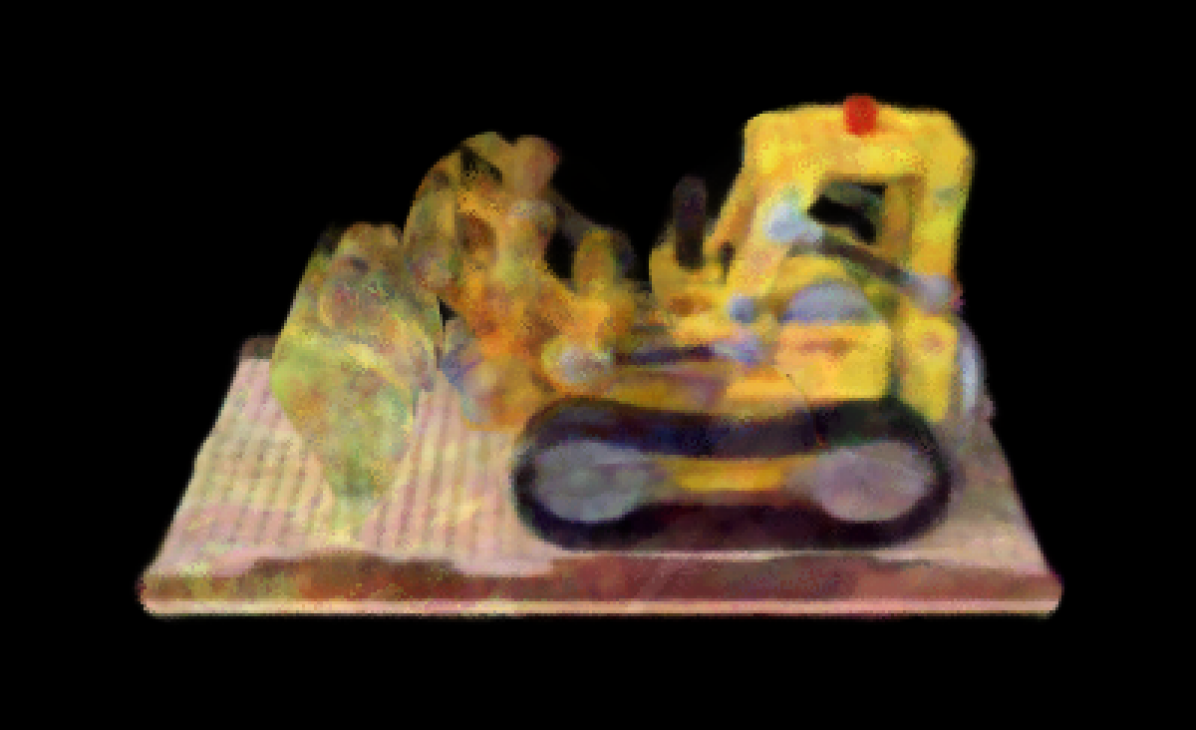
Namely, we use the $m$-th NeRF to render ray $r$ if it is assigned to the $m$-th part. If a ray is not associated with any part its color is black. The hard ray-part assignment is an essential property that ensures that editing one part does not alter the appearance of other parts (see Fig. 5).

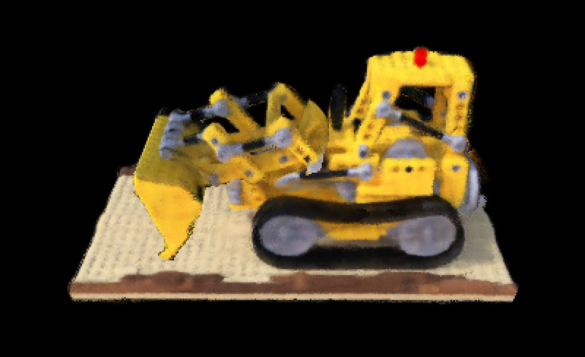
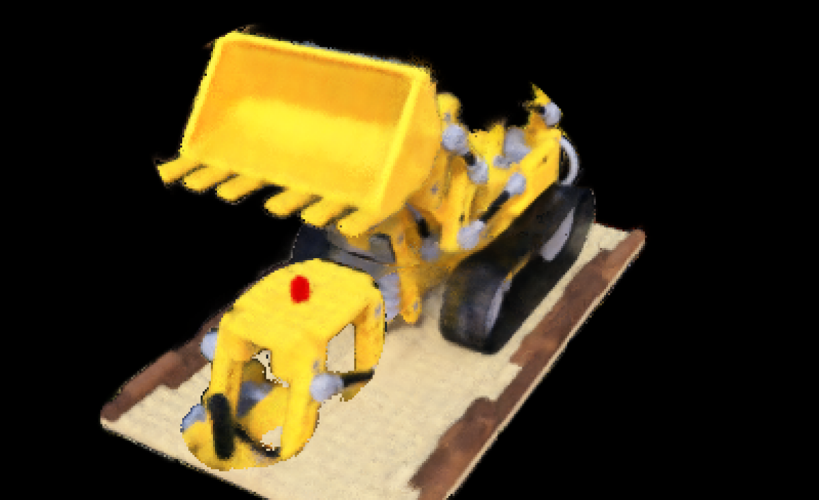
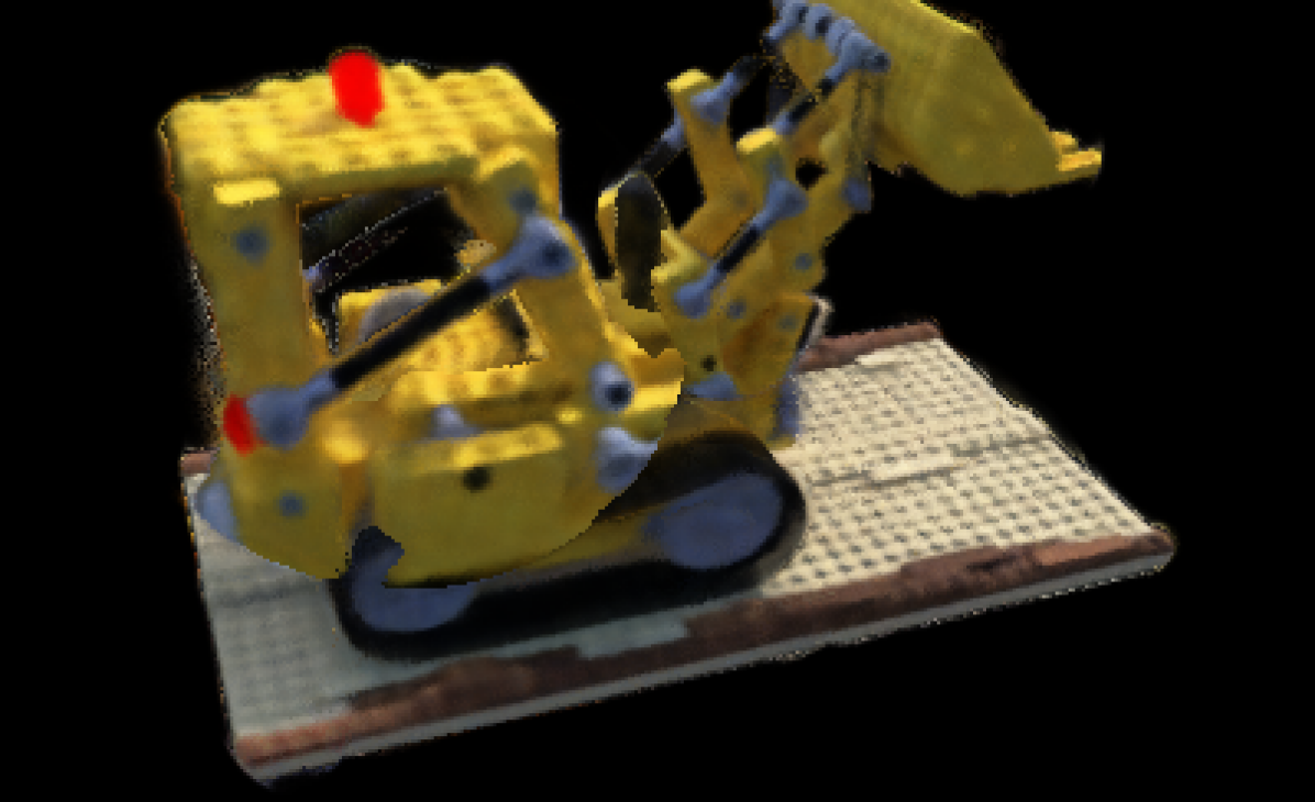
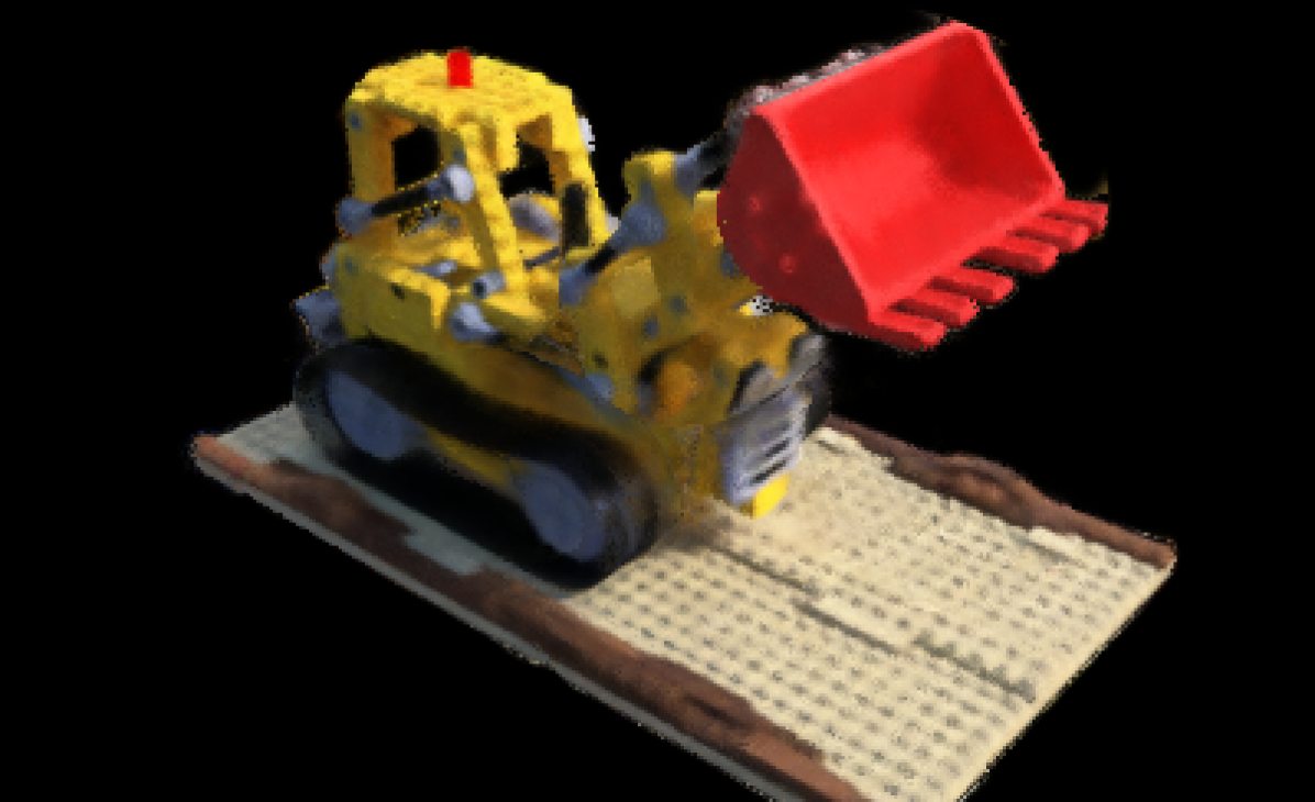
No Editing

Rotation

Translation

Scaling

Color

Figure 4: Scene-Specific Editing. The top and bottom row show the rendered images and the part-based geometries respectively. The 1st column shows the tractor from a novel view, before editing. In the 2nd, we select the bucket and rotate it downwards, whereas in the 3rd we translate the cockpit to the floor. In the 4th, we perform isotropic scaling of the cockpit and in the last we change the color of the bucket to red.

3.3 Network Architecture

We implement PartNeRF using an auto-decoder [6, 91]. The input to our model is two learnable embeddings $\mathbf{z}^{s},\mathbf{z}^{t}$, per training sample, that represent its shape and texture. Our network consists of three components: (i) the decomposition network that maps $\mathbf{z}^{s}$ and $\mathbf{z}^{t}$ to $M$ latent codes that control the per-part shape and texture, (ii) the structure network that predicts the pose and the scale for each part $m$ and (iii) the neural rendering network that renders a 2D image using the $M$ locally defined NeRFs. The overall architecture is illustrated in Fig. 2.

Decomposition Network: The decomposition network takes the two object specific embeddings $\mathbf{z}^{s},\mathbf{z}^{t}\in\mathbb{R}^{L_{d}}$ and maps them to $M$ per-part embeddings of the same dimensionality, $L_{d}$, using $M$ linear projections $f_{\theta}(\cdot)$. Subsequently, these embeddings are mapped to part-specific latent codes using two multi-head attention transformers, $\tau^{s}_{\theta}$ and $\tau^{t}_{\theta}$ without positional encoding [117] as follows

$$\{\mathbf{z}_{m}^{s}\}_{m=1}^{M} =\tau^{s}_{\theta}(f_{\theta}(\mathbf{z}^{s}))$$ (11)

$$\{\mathbf{z}_{m}^{t}\}_{m=1}^{M} =\tau^{t}_{\theta}(f_{\theta}(\mathbf{z}^{t})).$$ (12)

$\{\mathbf{z}_{m}^{s}\}_{m=1}^{M}$ and $\{\mathbf{z}_{m}^{t}\}_{m=1}^{M}$ are the latent codes that control the shape and texture of each part respectively.

Structure Network: The structure network $s_{\theta}$ maps the shape latent code $\mathbf{z}_{m}^{s}\in\mathbb{R}^{L_{d}}$ to a translation vector $\mathbf{t}_{m}\in\mathbb{R}^{3}$, a rotation matrix $\mathbf{R}_{m}\in SO(3)$ and a scale vector $\mathbf{s}_{m}\in\mathbb{R}^{3}$, with

$$\{\mathbf{t}_{m},\mathbf{R}_{m},\mathbf{s}_{m}\}=s_{\theta}(\mathbf{z}_{m}^{s})$$ (13)

an MLP shared across parts. Similar to [93], we parametrize $\mathbf{R}_{m}$ using quaternions [36]. As discussed in Sec. 3.2, we determine the set of rays $\mathcal{R}_{m}$ that are assigned to each part $m$ from (9) and transform them to its coordinate system.

Neural Rendering: Given the transformed points to the per-part coordinate system, we predict colors and occupancies with (5)$+$(3). Next, we perform volumetric rendering using (7) and render the object using $M$ NeRFs with (10).

No Editing

Rotation

Translation

Scaling

Figure 5: Soft Ray-Part Assignment. We demonstrate that enforcing a soft ray-part assignment results in parts that do not preserve their texture across transformations.

3.4 Training

Our optimization objective $\mathcal{L}$ is the sum over six terms combined with two regularizers on the shape and texture embeddings $\mathbf{z}^{s},\mathbf{z}^{t}$, namely

$$\mathcal{L}=\ \mathcal{L}_{rgb}(\mathcal{R})+\mathcal{L}_{mask}(\mathcal{R})+\mathcal{L}_{occ}(\mathcal{R})+\mathcal{L}_{cov}(\mathcal{R})\ +$$

$$\mathcal{L}_{overlap}(\mathcal{R})+\mathcal{L}_{control}+\left\|{\mathbf{z}^{s}}\right\|_{2}+\left\|{\mathbf{z}^{t}}\right\|_{2}.$$ (14)

As supervision, we use the observed RGB color $C(r)\in\mathbb{R}^{3}$ and the object mask $I(r)\in\{0,1\}$ for each ray $r\in\mathcal{R}$. We also associate $r$ with a binary label $\ell_{r}=I(r)$. Namely, we label a ray $r$ as inside, if $\ell_{r}=1$ and outside if $\ell_{r}=0$.

Reconstruction Loss: We measure the error between the observed $C(r)$ and the rendered $\hat{C}(r)$ color for the ray $r$ as

$$\mathcal{L}_{rgb}(\mathcal{R})=\sum_{r\in\mathcal{R}}\|\hat{C}(r)-C(r)\|_{2}^{2}.$$ (15)

Mask Loss: Likewise, we measure the squared error between the observed $I(r)$ and the rendered $\hat{I}(r)$ pixel value of the object mask for ray $r$ as

$$\mathcal{L}_{mask}(\mathcal{R})=\sum_{r\in\mathcal{R}}\|\hat{I}(r)-I(r)\|_{2}^{2}.$$ (16)

Note that $\hat{I}(r)$ can be derived from (10)$+$(7) simply by omitting the multiplication with the predicted color, namely

$$\hat{I}(r)=\sum_{m=1}^{M}\mathbbm{1}_{r\in\mathcal{R}_{m}}\sum_{i=1}^{N}h_{\theta}^{m}(\mathbf{x}_{i}^{r})\prod_{j<i}\left(1-h_{\theta}^{m}(\mathbf{x}_{j}^{r})\right).$$ (17)

Occupancy Loss: This loss makes sure that the generated parts do not occupy empty space. To this end, we employ a binary cross-entropy classification loss $\mathcal{L}_{ce}(\cdot;\cdot)$ between the predicted and the target labels for all rays

$$\mathcal{L}_{occ}(\mathcal{R})=\frac{1}{|\mathcal{R}|}\sum_{r\in\mathcal{R}}\Big{(}\mathcal{L}_{ce}(\hat{\ell}_{r},\ell_{r})+\mathcal{L}_{ce}(\tilde{\ell}_{r},\ell_{r})\Big{)},$$ (18)

where $\hat{\ell}_{r}$ and $\tilde{\ell_{r}}$ are the predicted labels along ray $r$ based on the predicted occupancies and ellipsoid occupancies respectively. Intuitively, we consider a ray $r$ to be inside the object if it is inside at least one part. In turn, in order for $r$ to be inside a part it suffices if at least one point along the ray $\mathcal{X}_{r}$ is inside this part. This can be expressed as

$$\hat{\ell}_{r} =\max_{m\in\{1\dots M\}}\max_{\mathbf{x}_{i}^{r}\in\mathcal{X}_{r}}h_{\theta}^{m}(\mathbf{x}_{i}^{r})$$ (19)

$$\tilde{\ell}_{r} =\max_{m\in\{1\dots M\}}\max_{\mathbf{x}_{i}^{r}\in\mathcal{X}_{r}}g_{\theta}^{m}(\mathbf{x}_{i}^{r}).$$ (20)

.

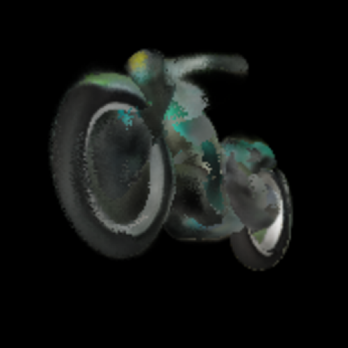
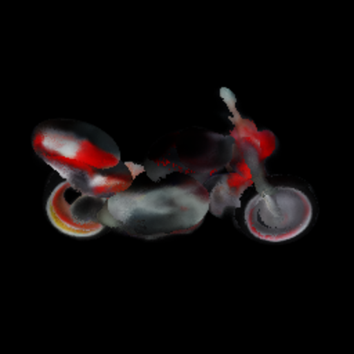
Motorbike

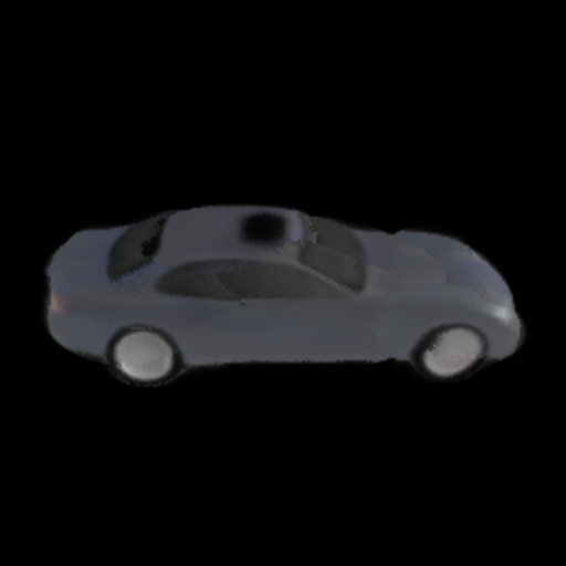
Car

Chair

Pi-GAN

GRAF

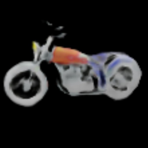
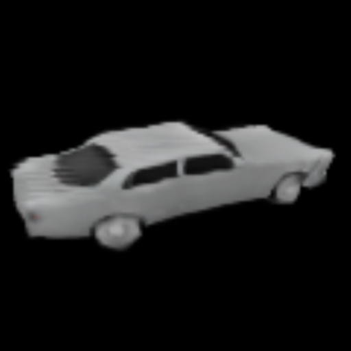
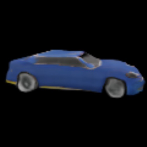
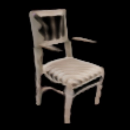
EG3D

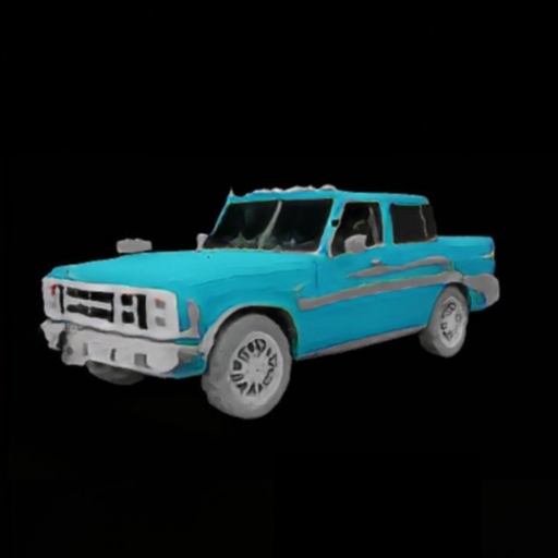
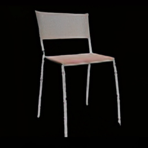
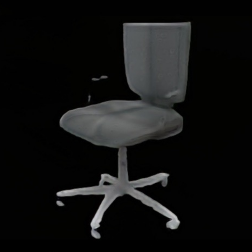
GET3D

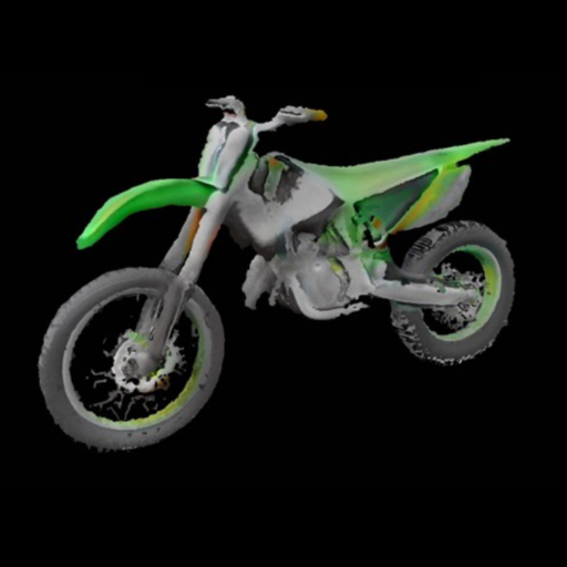
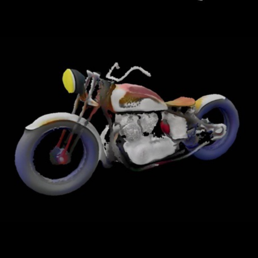
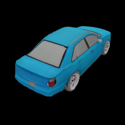
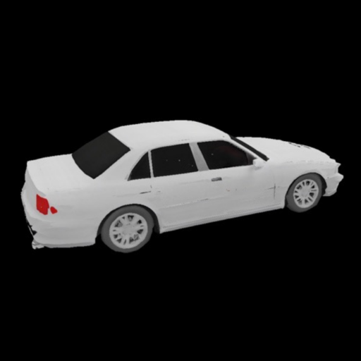
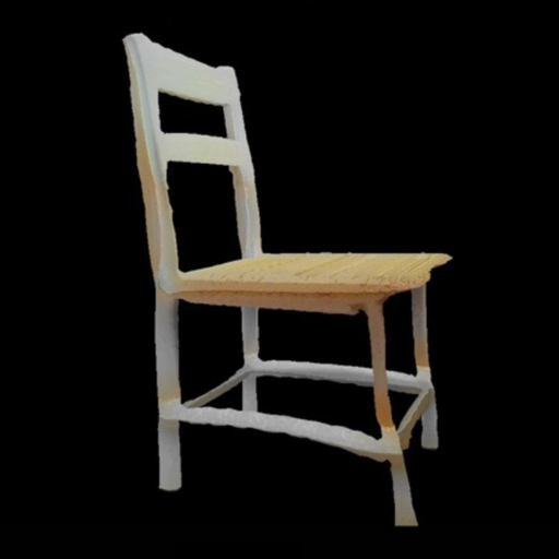
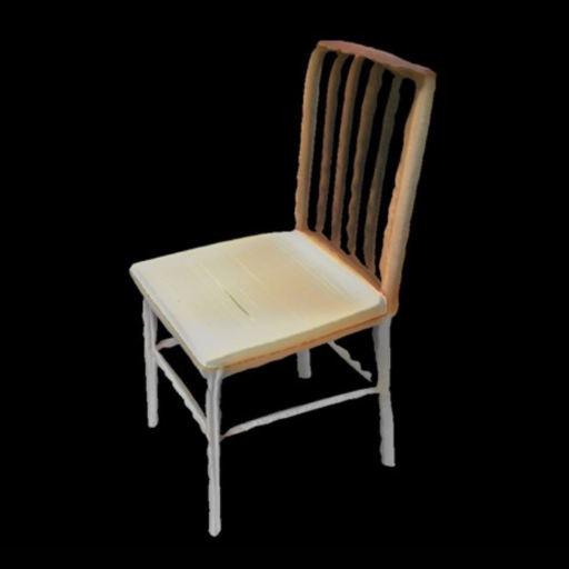
Ours

Figure 6: Shape Generation. We compare our model with 3D generative models that are part agnostic but can generate textured meshes. Here we show two randomly generated samples per category.

Method	Rendering	MMD-CD ($\downarrow$)			COV-CD ($\%,\uparrow$)
		Motorbike	Car	Chair	Motorbike	Car	Chair
GET3D	Differentiable	1.72	0.71	3.72	67.12	58.39	69.91
Pi-GAN	Volumetric	21.80	25.54	6.65	6.85	0.55	39.65
GRAF	Volumetric	2.40	10.63	6.80	50.68	1.57	39.28
EG3D	Volumetric	2.21	0.72	4.72	34.25	49.52	50.14
Ours	Volumetric	1.68	1.74	4.42	56.06	21.10	67.20

Table 1: Comparison with 3D Generative Models. We measure MMD-CD ($\downarrow$) and COV-CD ($\uparrow$). Note that none of these baselines considers parts nor allows any part-level shape editing.

Coverage Loss: This loss ensures that the parts cover the object, thus preventing degenerate arrangements with small parts or parts outside the object. To implement this, we encourage parts to contain at least $k$ inside rays. This can be expressed as a binary cross-entropy loss between the predicted per-part and target labels for all rays in $\mathcal{R}_{m}^{k}$,

$$\mathcal{L}_{cov}(\mathcal{R})=\frac{1}{M}\sum_{m=1}^{M}\sum_{r\in\mathcal{R}_{m}^{k}}\mathcal{L}_{ce}(\hat{\ell}_{r}^{m},\ell_{r}),$$ (21)

where $\displaystyle\hat{\ell}_{r}^{m}=\max_{\mathbf{x}_{i}^{r}\in\mathcal{X}_{r}}h_{\theta}^{m}(\mathbf{x}_{i}^{r})$ the predicted label for ray $r$ wrt. part $m$ and $\mathcal{R}_{m}^{k}$ the set of the $k$ inside rays with the greatest predicted occupancy values for this part.

Overlapping Loss: To encourage the generated parts to capture different regions of the object, we penalize rays that are inside of more than $\lambda$ parts as follows

$$\mathcal{L}_{overlap}(\mathcal{R})=\frac{1}{|\mathcal{R}|}\sum_{r\in\mathcal{R}}\max\Big{(}0,\sum_{m=1}^{M}\hat{\ell}_{r}^{m}-\lambda\Big{)}.$$ (22)

Control Loss: To ensure uniform control across the shape, we want parts with comparable volumes. We implement this loss on the volumes $\mathcal{V}(\cdot)$ of the ellipsoids, as follows:

$$\mathcal{L}_{control}=\frac{1}{M(M-1)}\sum_{i=1}^{M}\sum_{j=1}^{i}|\mathcal{V}(\mathbf{s}_{i})-\mathcal{V}(\mathbf{s}_{j})|.$$ (23)

Tables

Airplanes

SPAGHETTI [44]

Ours

Ours with Parts

Figure 7: Shape Generation. We compare our model with [44] and show three randomly generated samples per category.

Method	Supervision	MMD-CD ($\downarrow$)		COV-CD ($\%,\uparrow$)
		Airplane	Table	Airplane	Table
DualSDF	3D Shapes	4.20	12.30	25.00	36.30
SPAGHETTI	3D Shapes	2.40	5.90	35.00	47.80
Ours	Multi-view	1.37	4.48	37.90	40.60

Table 2: Comparison with Part-based Generative Models. We measure MMD-CD ($\downarrow$) and the COV-CD ($\uparrow$). Unlike our model, both [37, 44] require 3D supervision during training.

4 Experimental Evaluation

We provide an extensive evaluation of PartNeRF comparing it to relevant baselines in terms of the realism and diversity of the generated shapes. We also showcase several editing operations of our model on multiple object categories. Additional results, ablations and implementation details are provided in the supplementary.

Datasets: We use five ShapeNet [11] categories: Motorbike, Chair, Table, Airplane and Car. To render our training data, we randomly sample camera poses from the upper hemisphere of each shape and render images at $256^{2}$ resolution as in [27]. For the Car, Table, Airplane and Chair, we use $24$ random views, while for Motorbike we use $100$. To ensure fair comparison with our baselines, we use the train-test splits of [27] for the Motorbike, Car, Chair object categories and the train-test splits of [44] for the Airplane, Table category. In all our experiments, we perform category specific training. Finally, we showcase the scene-specific editing capabilities of our model on the Lego tractor [76]. In all our experiments, we set $M=16$.

Baselines: We compare our model with several NeRF-based models: GRAF [105], Pi-GAN [10], EG3D [9] and the concurrent GET3D [27] that relies on differentiable rendering. Unlike our model, none of the above considers parts. We also compare with the part-based DualSDF [37] and SPAGHETTI [44] that require 3D supervision.

Metrics: We report the Coverage (COV) and the Minimum Matching Distance (MMD) [1] using Chamfer-$L_{2}$ distance. MMD measures how likely it is that a generated shape looks like a test shape. COV measures how many shape variations are covered by the generated shapes.

4.1 Scene-Specific Shape Editing

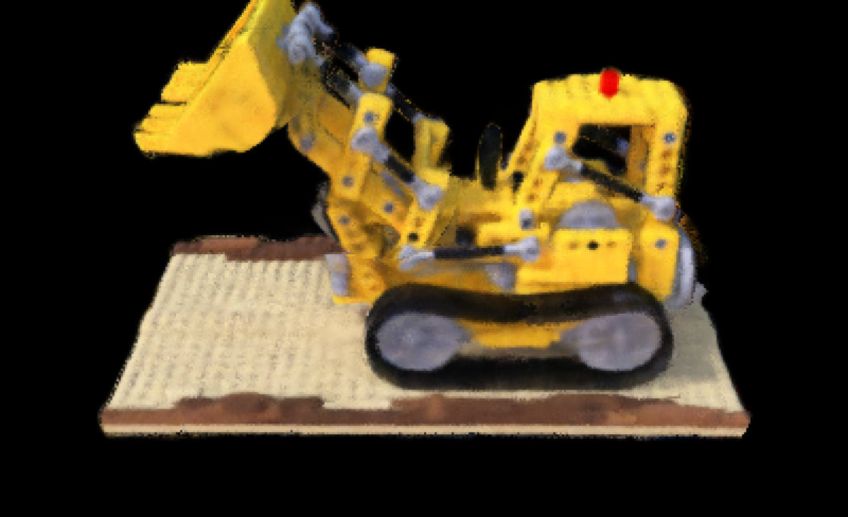
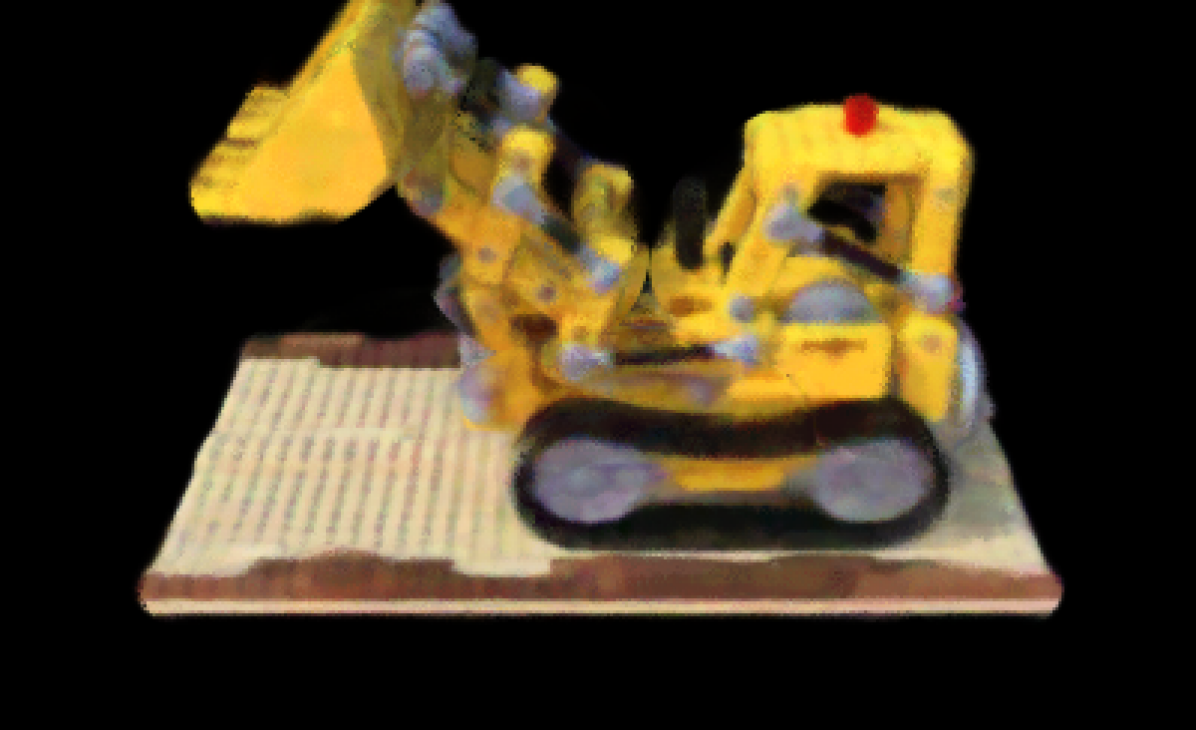
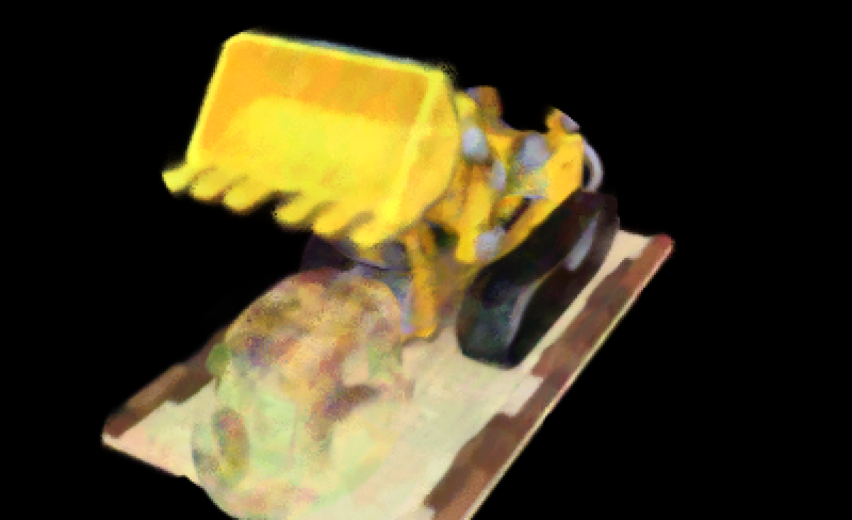
We train PartNeRF on the tractor scene [76], using all $200$ training views. The results are shown in Fig. 4. Initially, we select the part that corresponds to the bucket of the tractor and apply a rotation, such that the bucket is facing downwards. Similarly, we select the cockpit and move it to a new location on the floor, by adding a displacement to the part’s translation vector. During both transformations the rest of the shape (geometry, parts and textures) does not alter. We then apply a non-rigid transformation on the cockpit, scaling it uniformly across all axes, by multiplying the part’s rotation with an isometric scale matrix. Again, while we change the shape of one part its texture as well as the texture and shape of the others does not change. Finally, we alter the color of the bucket by explicitly setting the predicted color of its associated NeRF to red.

Figure 8: Shape Interpolation. From left to right, we interpolate between the geometry and texture latent codes of the two shapes.

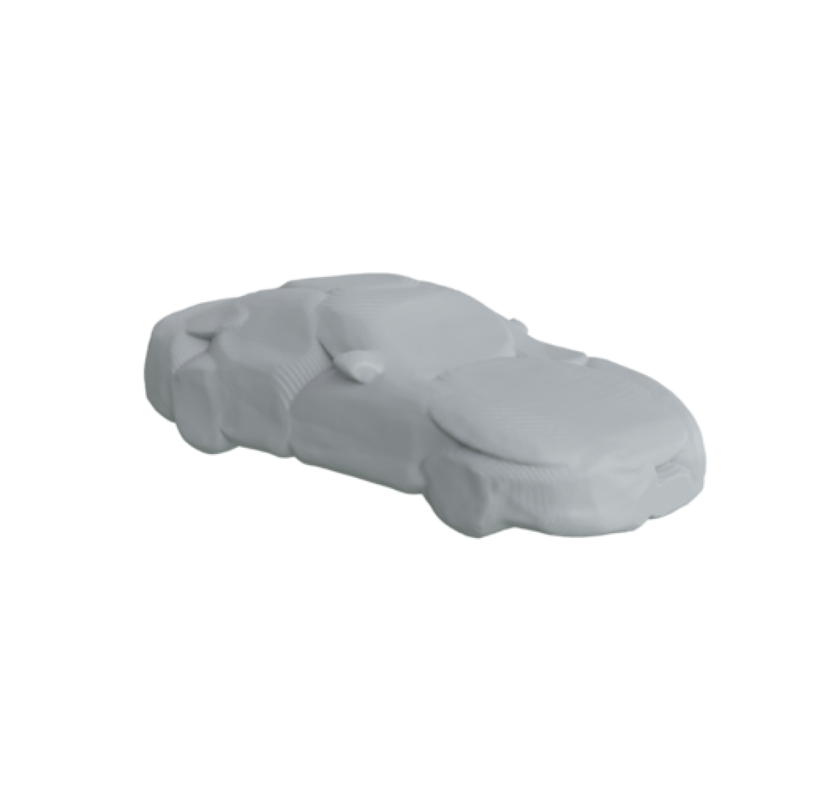
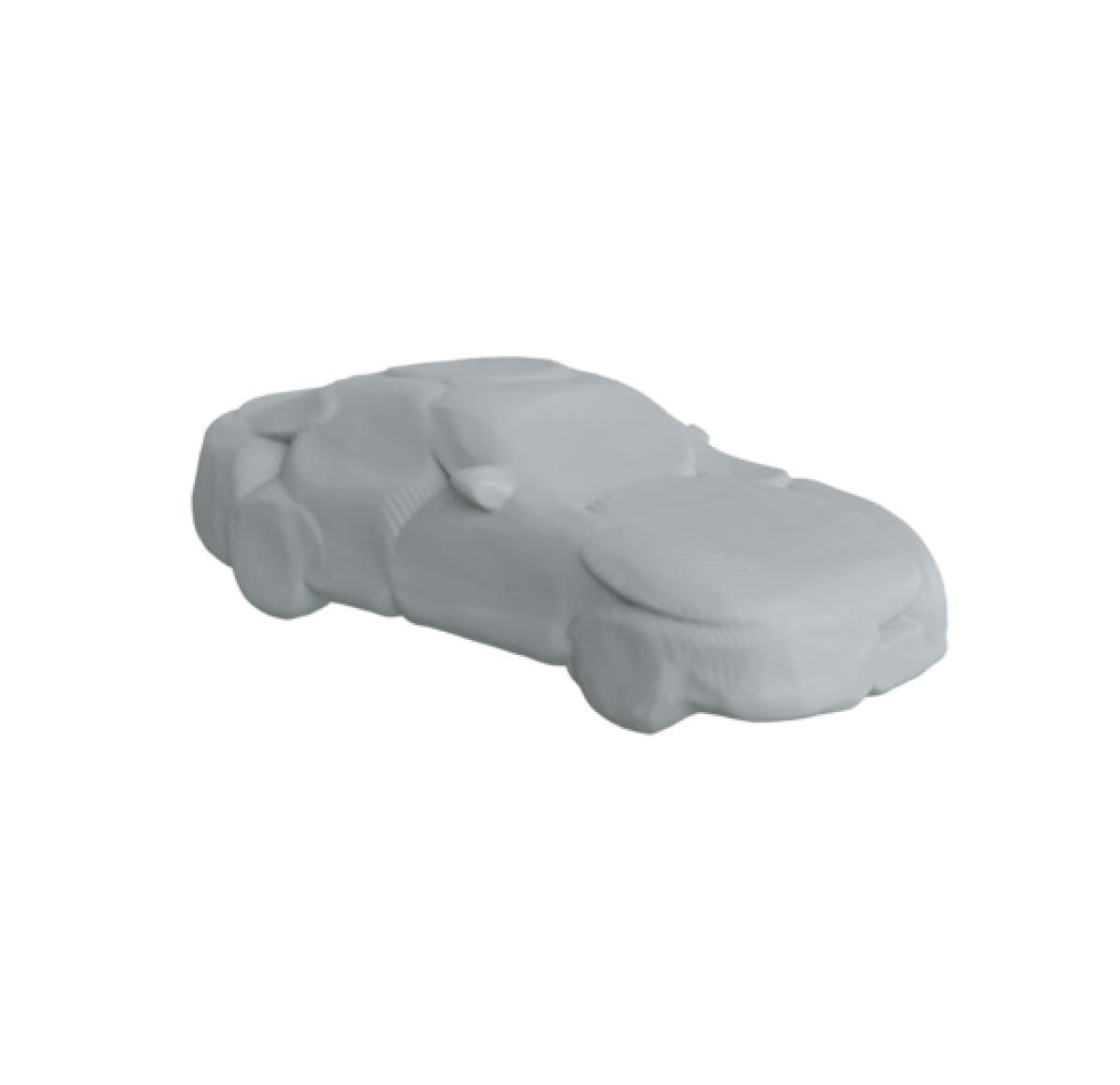
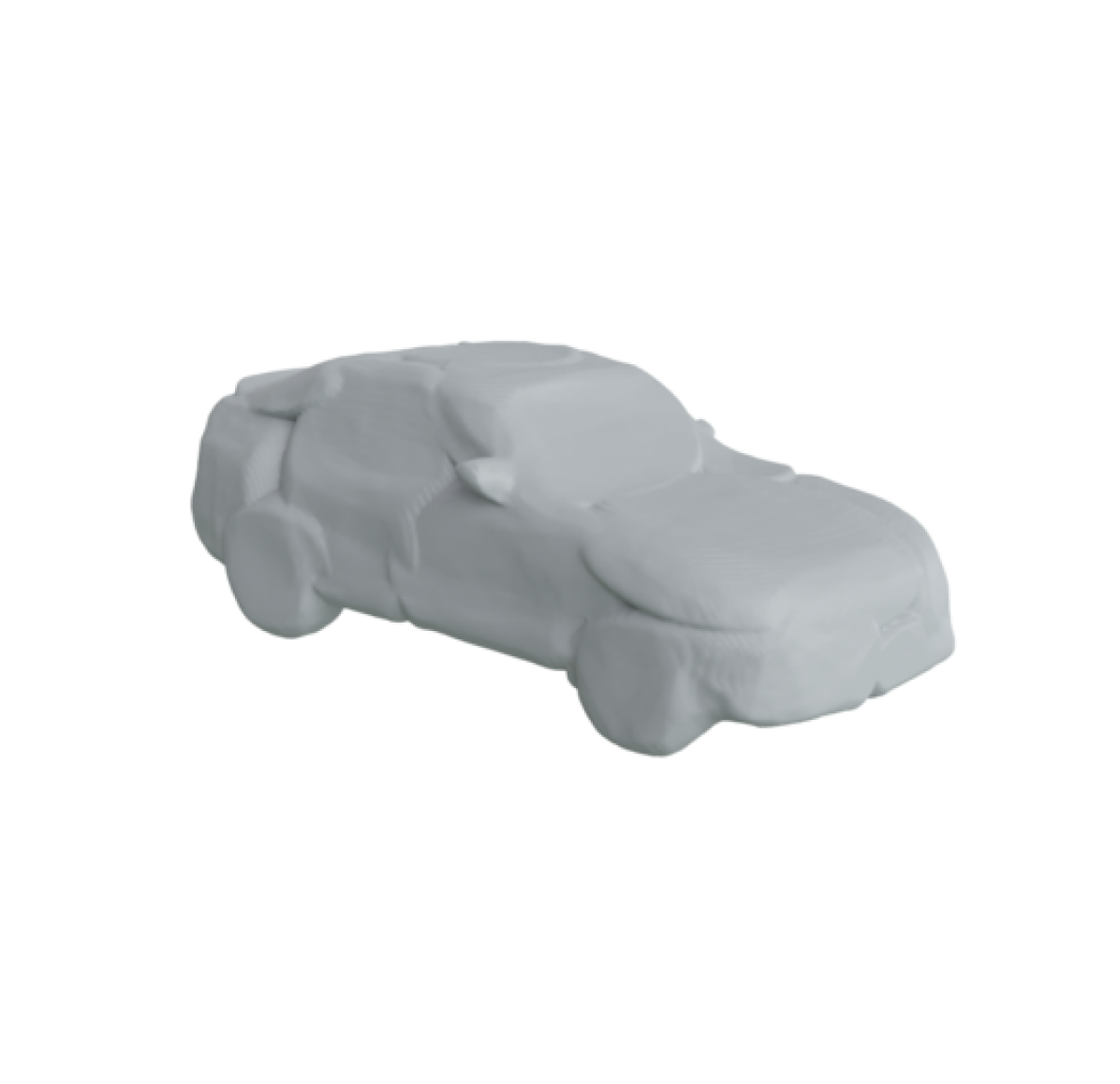
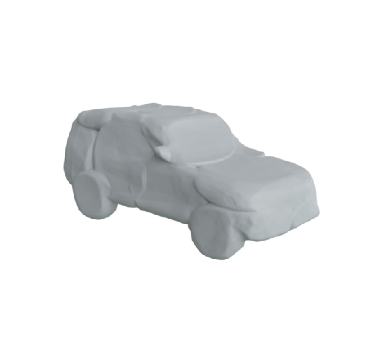
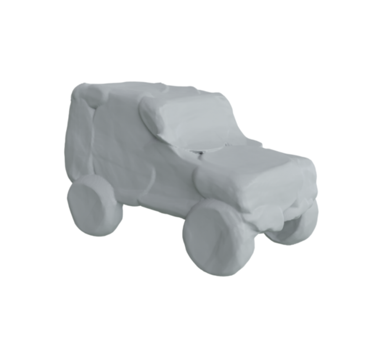
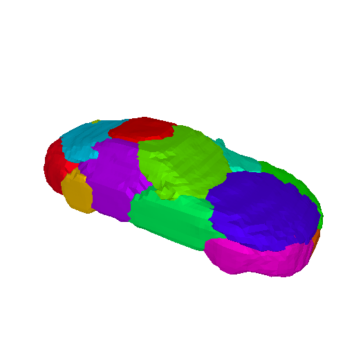
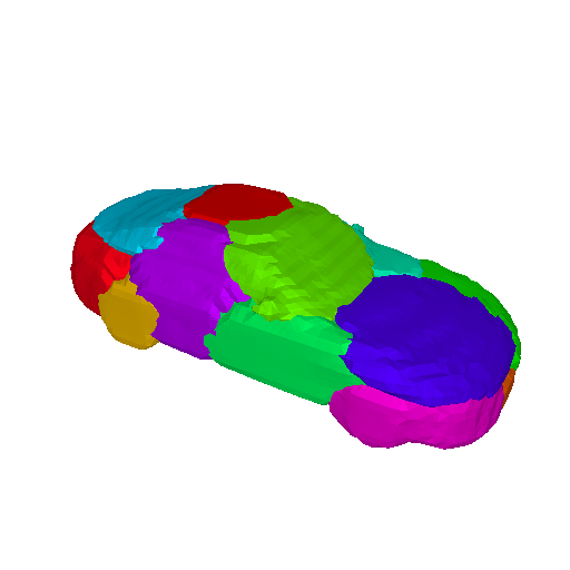
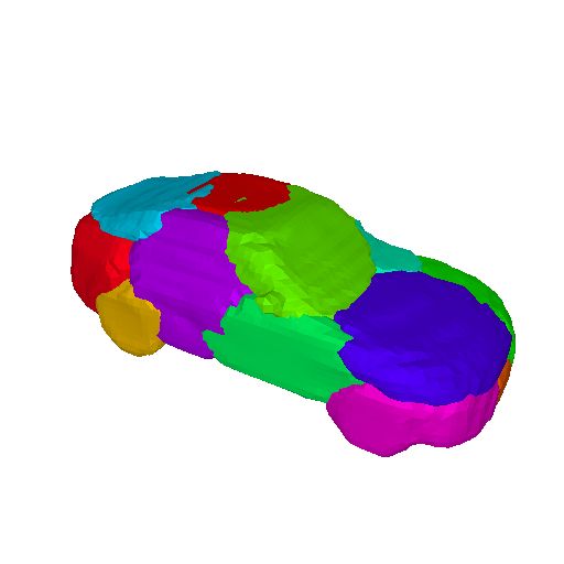
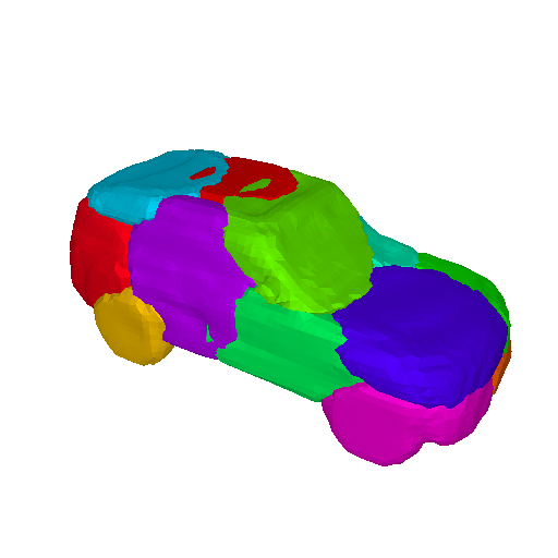
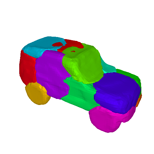
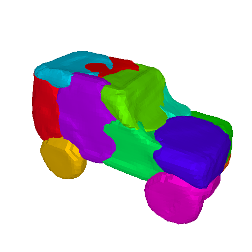
Soft Ray-Part Assignment: To investigate the impact of our hard ray-part assignment, we train a variant of our model without, namely the color of a ray can be determined from multiple NeRFs. We note that when we apply a transformation on a part of the object, also the color of other parts changes, as illustrated in Fig. 5. Moreover, note that with this variant of our model it is not possible to change the color of specific parts of the generated object, as in Fig. 4.

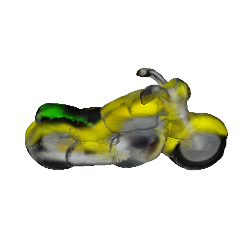
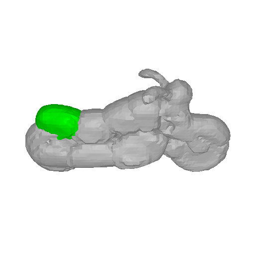
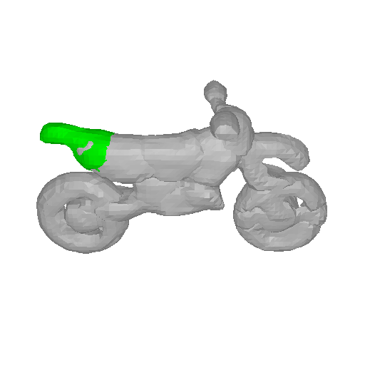
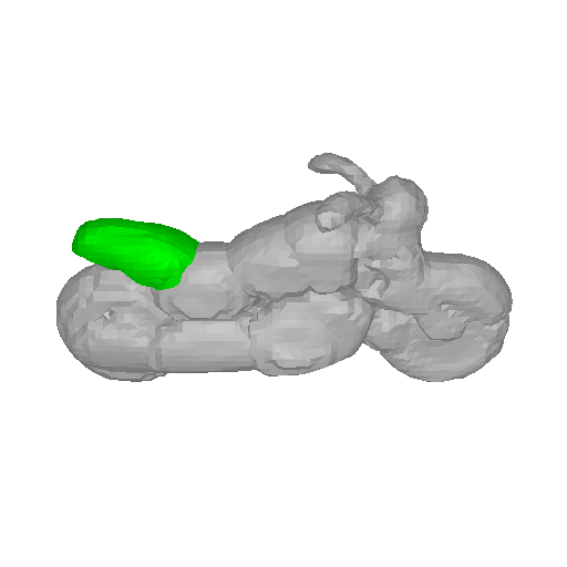
Shape 1

Shape 2

Shape Code Interpolation

Texture Code Interpolation

Figure 9: Part-Level Interpolation. From left to right, we interpolate between two parts (colored in green) from two shapes. For the motorbikes, we select the saddle and for the airplanes the right wing. In the 3rd and 4th columns, we interpolate between the shape codes of the two parts, whereas in the 5th and 6th we interpolate between the texture codes of the two parts.

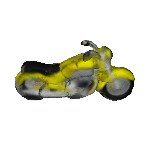
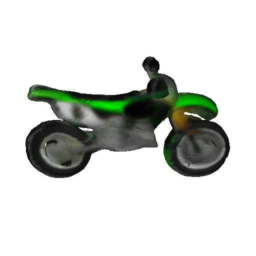
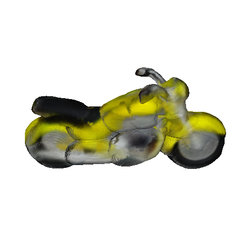
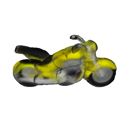
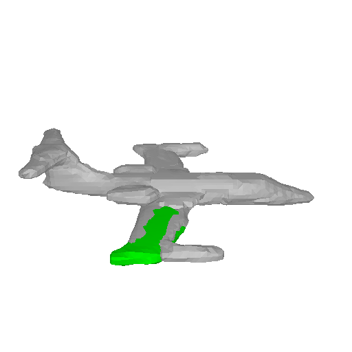
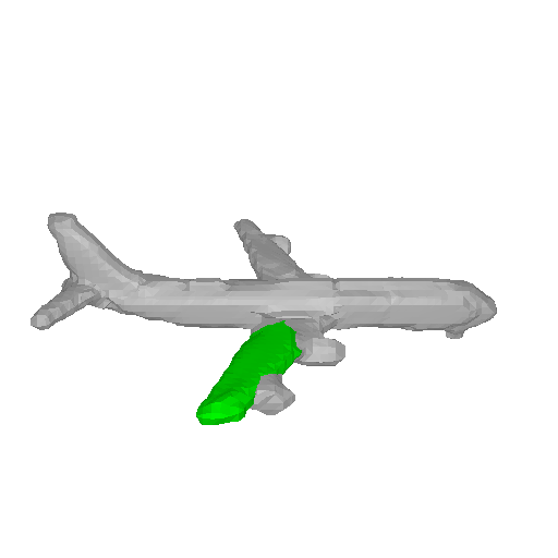
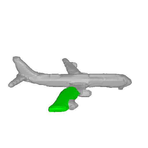
4.2 Shape Generation

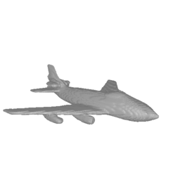
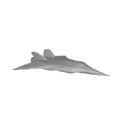
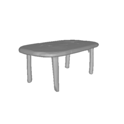
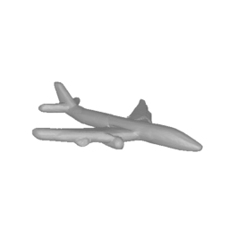
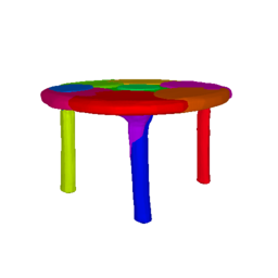
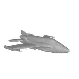
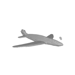
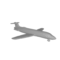
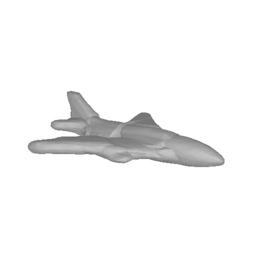
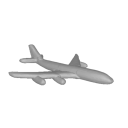
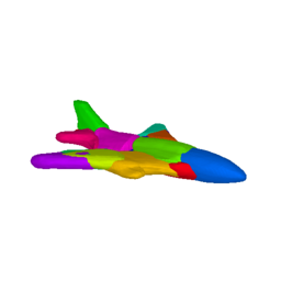
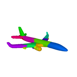
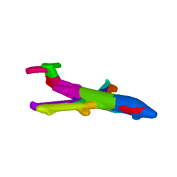
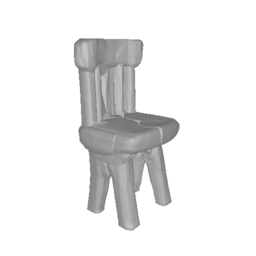
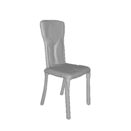
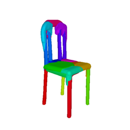
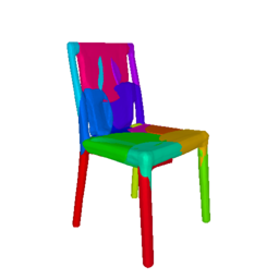
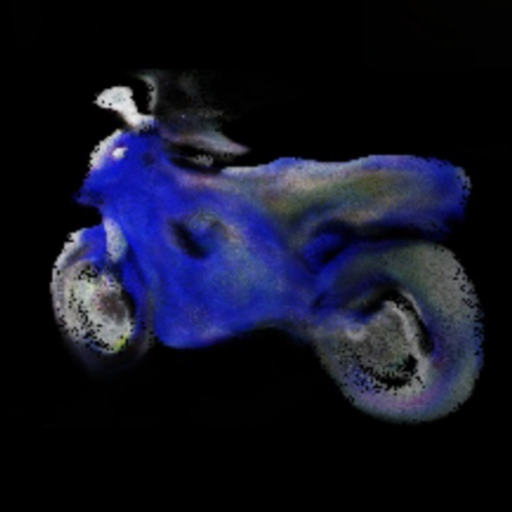
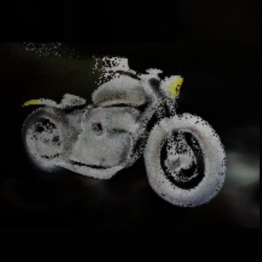
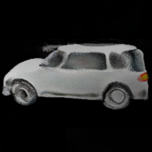
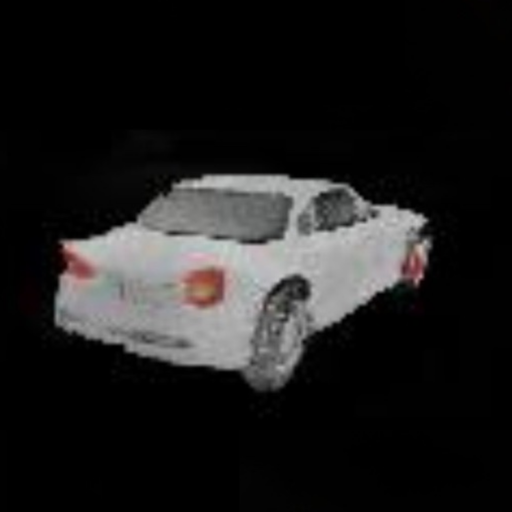
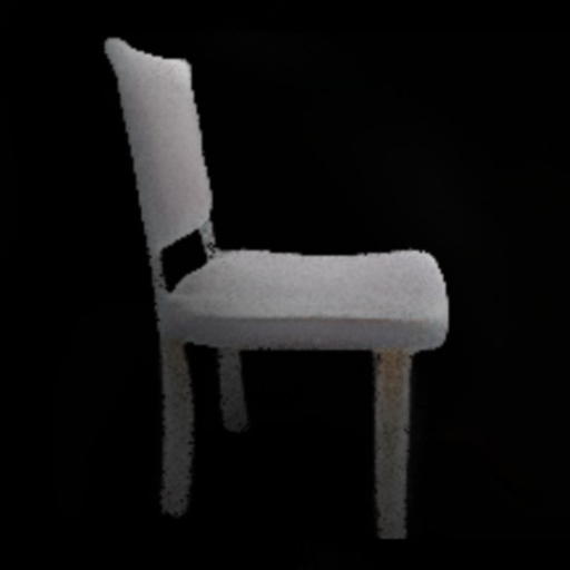
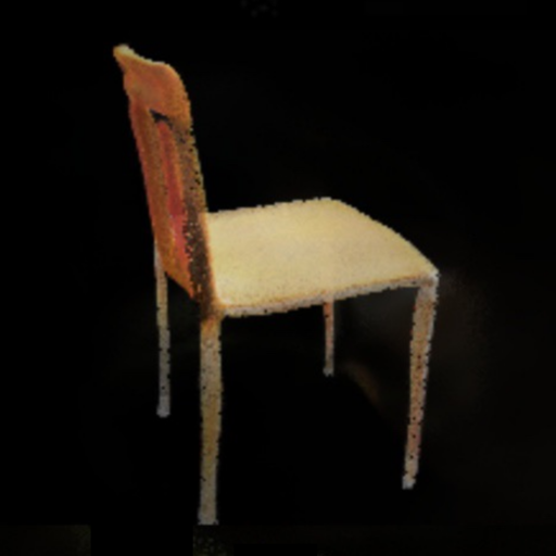
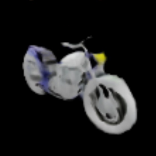
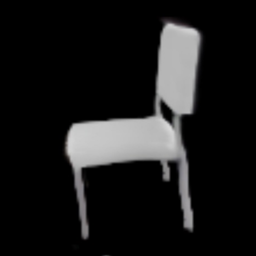
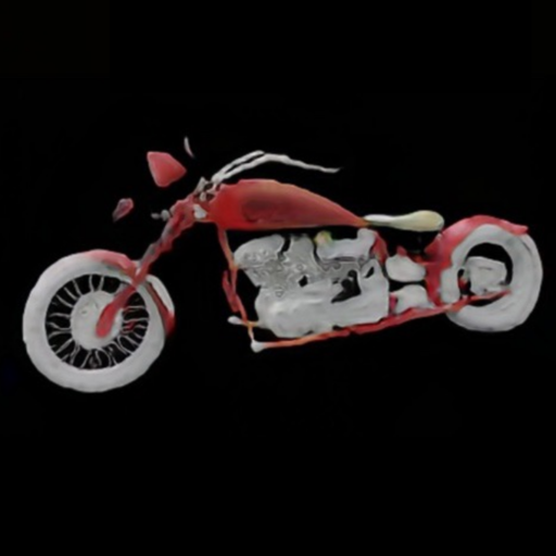
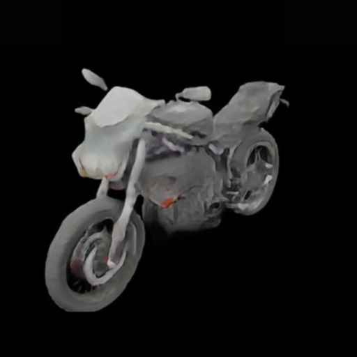
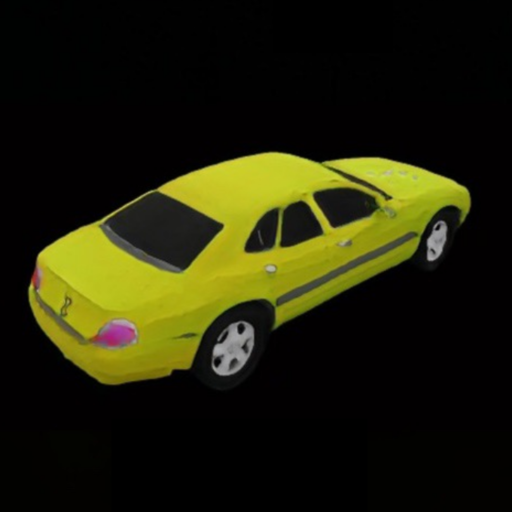
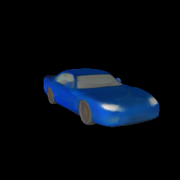
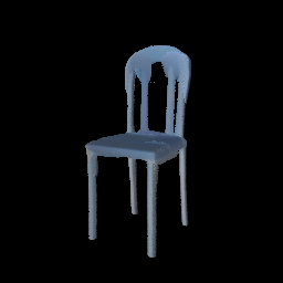
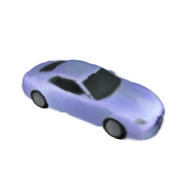
In Tab. 1, we compare the quality of our generations with NeRF-based generative models and observe that it outperforms existing approaches in terms of MMD and COV on Motorbikes and Chairs, while being better than [105, 10] also for Cars. Furthermore, it performs on par with the concurrent work of [27] that relies on a highly optimized differentiable graphics renderer [58] and requires training for approximately 16 GPU days (8 A100 for 2 days). Instead our model employs a simpler volumetric renderer and training takes approximately 5 GPU days (1 RTX 3090). Compared to [10, 105], our generations are sharper with more crisp colors (see Fig. 6). However, compared to [27, 9] that employ tri-plane representations and hence can generate high-resolution textures, our textures are less detailed.

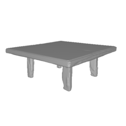
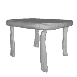
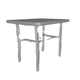
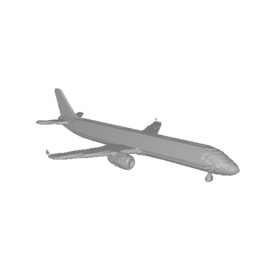
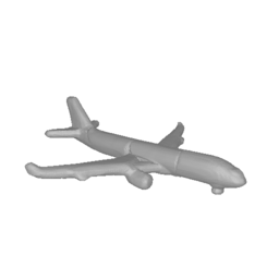
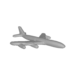
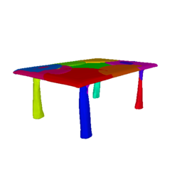
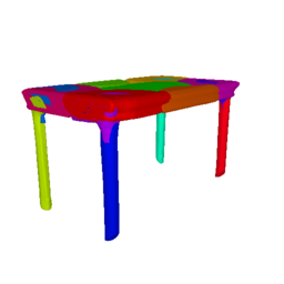
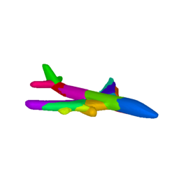
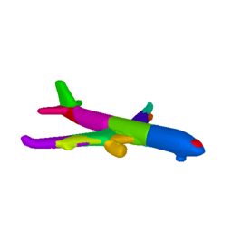
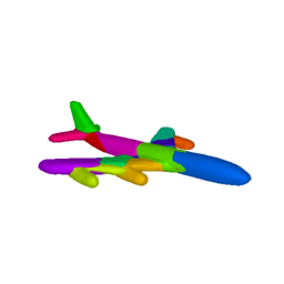
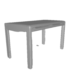
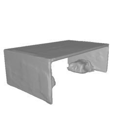
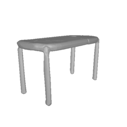
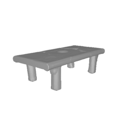
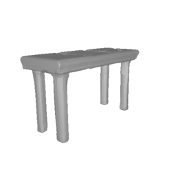
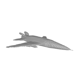
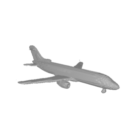
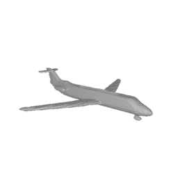
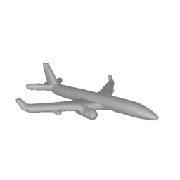
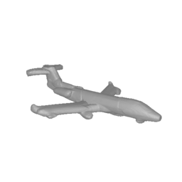
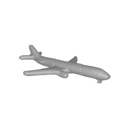
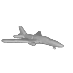
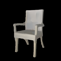
We also compare PartNeRF with state-of-the-art part-based approaches that require 3D supervision. While our model is trained from posed images and object masks, it consistently generates plausible 3D geometries (see Fig. 7). This is also valitated quantitatively in Tab. 2, where we observe that our model outperforms both [37, 44] on Airplanes while being better in terms of MMD for Tables.

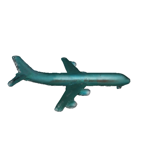
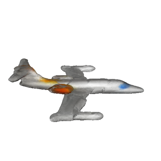
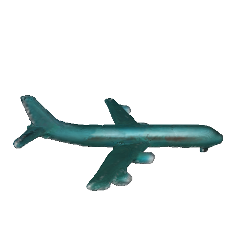
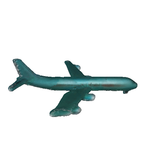
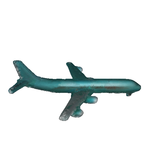
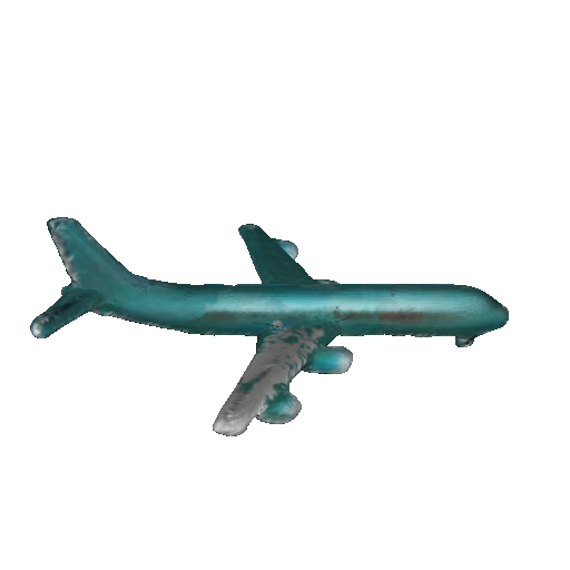
Shape Interpolation: In Fig. 8, from left to right, we show interpolations between the shape and texture codes of two cars. We observe that our model smoothly interpolates between two shapes, while preserving the shape structure and the the part-based structure.

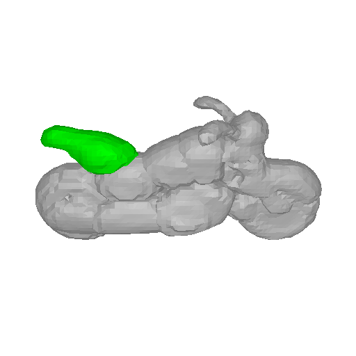
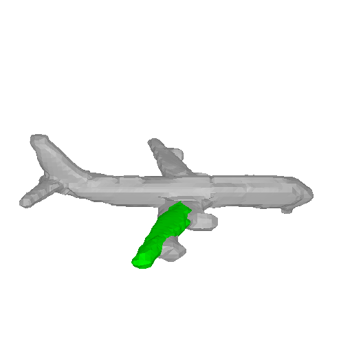
Part-level Interpolation: Fig. 9 shows part-level interpolation, where we pick two shapes and select a part from both. For the motorbikes, we choose the saddle part and linearly interpolate its shape and texture codes. We repeat for the airplanes, where we select the right wing. When we interpolate the shape codes, the geometry changes, while the texture remains the same. In contrast, when we interpolate the texture codes, the geometry remains unchanged and only the part texture changes smoothly. Across all interpolations our model consistently generates realistic shapes.

4.3 Shape and Texture Editing

Shape Mixing: Starting from two shapes, the task is to select and combine parts in a meaningful way. As shown in Fig. 10, we consider two types of mixing operations: geometry and texture mixing. In geometry mixing, we combine parts from two objects and generate a new one, whose texture is determined by the texture codes from one of the two, while shape codes are taken from different parts of the two objects (third column). In texture mixing, we mix the shapes only in terms of texture, while the shape is determined by the shape codes of one object (fourth column). We also combine both mixing modes. PartNeRF consistently generates plausible shapes across all editing operations.

Shape 1

Shape 2

Geometry Mixing

Texture Mixing

Combined

Figure 10: Shape Mixing. We mix parts from two shapes and show geometry (3rd column), texture (4th column), and combined geometry and texture mixing (5th column). The selected parts for mixing are colored in green.

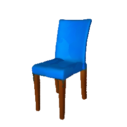
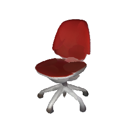
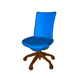
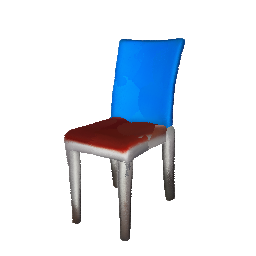
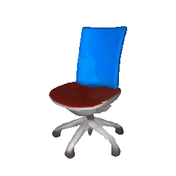
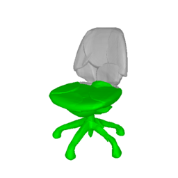
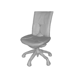
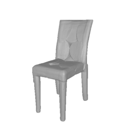
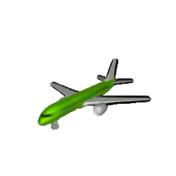
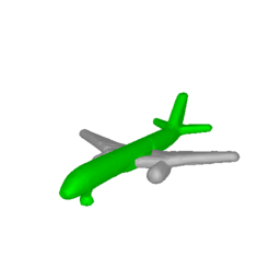
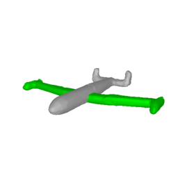
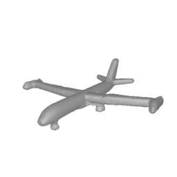
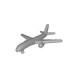
Shape Editing: Our method also allows several shape editing operations on the part level, such as applying rigid and non-rigid transformations and inserting or removing parts. Affine transformations are directly applied on the rotation and translation vector that define the per-part coordinate frame. To remove a part, it suffices to ignore its associated NeRF in the rendering process. Likewise, adding a part amounts to incorporating its NeRF during rendering. Examples of these operations are summarized in Fig. 1.

5 Conclusion

In this paper, we introduce PartNeRF, the first part-aware generative model that parametrizes parts as NeRFs. As our work considers the decomposition of objects into parts, it enables intuitive part-level control and several editing operations not previously possible. Furthermore, it is trained without explicit 3D supervision, using only posed images and object masks. Our experiments showcase the ability of our model to generate plausible 3D shapes with texture. Moreover, we demonstrate several editing operations both on the texture and the shape of the generated object. In future work, we plan to investigate incorporating more complex representations such as triplanes [9], or using differentiable rendering techniques [27] in order to better represent the object’s texture. Another exciting direction for future research is extending our model to moving objects.

Appendix A Implementation Details

In this section, we provide a detailed description of the several components of our network architecture (Sec. A.1). Next, we describe our training procedure (Sec. A.2) and the generation protocol (Sec. A.3). Then, we provide details regarding the various editing operations demonstrated in the main submission (Sec. A.4). Finally, we detail our metrics computation (Sec. A.5) and discuss our baselines (Sec. A.6).

A.1 Network Architecture

Here, we describe the architecture of each individual component of our model, as illustrated in Fig. 2 in the main submission. As already discussed in Sec 3.3 of our main submission, we implement our generative model using an auto-decoder [6, 91]. In particular, the input to our model is a set of embedding vectors $\mathcal{Z}=\{\mathbf{z}_{i}\}_{i=1}^{n}$, uniquely identifying each one from the $n$ training samples. Each $\mathbf{z}_{i}=\{\mathbf{z}^{s},\mathbf{z}^{t}\}$, comprises two learnable embeddings that capture the shape and appearance properties of each sample. Note that both the shape $\mathbf{z}^{s}$ and texture $\mathbf{z}^{t}$ codes are initialized by sampling from the normal distribution $\mathbf{z}^{s},\mathbf{z}^{t}\sim N(\mathbf{0},I)$. To avoid notation clutter, we omit the object index $i$ in the rest of this section.

Our network consists of three main components: (i) the decomposition network that maps the instance-specific latent codes $\{\mathbf{z}^{s},\mathbf{z}^{t}\}$ to $M$ per-part shape $\{\mathbf{z}_{m}^{s}\}_{i=1}^{M}$ and texture $\{\mathbf{z}_{m}^{t}\}_{i=1}^{M}$ embeddings, (ii) the structure network that takes the per-part shape code $\mathbf{z}_{m}^{s}$ and predicts an affine transformation $\{\mathbf{R}_{m},\mathbf{t}_{m}\}$ and scale $\mathbf{s}_{m}$ that controls the pose and the area of influence of this part, and (iii) the neural rendering module that renders a 2D image using $M$ NeRFs. As supervision, we use the observed RGB color $C(r)\in\mathbb{R}^{3}$ and the object mask $I(r)\in\{0,1\}$ for each ray $r\in\mathcal{R}$. We also associate $r$ with a binary label $\ell_{r}=I(r)$, as shown in Fig. 15. Namely, we label a ray $r$ as inside, if $\ell_{r}=1$ and outside if $\ell_{r}=0$.

Decomposition Network: The decomposition network maps the instance-specific shape and texture $\{\mathbf{z}^{s},\mathbf{z}^{t}\}$ latent codes into a set of $M$ latent codes that control the shape and appearance of each part. We implement the decomposition network using two multi-head attention transformers without positional encoding [117], $\tau^{s}_{\theta}$ and $\tau^{t}_{\theta}$, that predict $M$ shape $\{\mathbf{z}_{m}^{s}\}_{m=1}^{M}$ and texture $\{\mathbf{z}_{m}^{t}\}_{m=1}^{M}$ codes, as follows:

$$\tau^{s}_{\theta}:\mathbb{R}^{L_{d}} \rightarrow\mathbb{R}^{L_{d}\times M} \{\mathbf{z}_{m}^{s}\}_{m=1}^{M} =\tau^{s}_{\theta}(f_{\theta}(\mathbf{z}^{s}))$$ (24)

$$\tau^{t}_{\theta}:\mathbb{R}^{L_{d}} \rightarrow\mathbb{R}^{L_{d}\times M} \{\mathbf{z}_{m}^{t}\}_{m=1}^{M} =\tau^{t}_{\theta}(f_{\theta}(\mathbf{z}^{t}))$$

where $L_{d}$ is the dimensionality of the instance-specific embeddings and is set to $128$. The input to transformer $\tau^{s}_{\theta}$ is the set of $M$ per-part shape codes $\{\hat{\mathbf{z}}^{s}\}_{m=1}^{M}$, where $\hat{\mathbf{z}}_{m}^{s}\in\mathbb{R}^{128}$. Likewise, the input to transformer $\tau^{t}_{\theta}$ is the set of $M$ per-part texture codes $\{\hat{\mathbf{z}}^{t}\}_{m=1}^{M}$, where $\hat{\mathbf{z}}_{m}^{t}\in\mathbb{R}^{128}$. Note that the $M$ shape $\{\hat{\mathbf{z}}^{s}\}_{m=1}^{M}$ and texture $\{\hat{\mathbf{z}}^{t}\}_{m=1}^{M}$ codes are produced from $\mathbf{z}_{s}$ and $\mathbf{z}_{t}$ respectively using $M$ linear projections $f_{\theta}(\cdot)$. The output of each transformer is the set of per-part shape $\{\mathbf{z}_{m}^{s}\}_{i=1}^{M}$ and texture $\{\mathbf{z}_{m}^{t}\}_{i=1}^{M}$, where $\mathbf{z}_{m}^{s}\in\mathbb{R}^{128}$ and $\mathbf{z}_{m}^{t}\in\mathbb{R}^{128}$. Both transformers consist of $2$ layers with $4$ attention heads. The queries, keys and values have 128 dimensions and the intermediate representations for the MLPs have 1024 dimensions. To implement the transformer architecture we use the transformer library provided by Wightman [122].

(a) $\tau^{s}_{\theta}(\cdot)$ predicts the $M$ per-part shape codes $\{\mathbf{z}_{m}^{s}\}_{i=1}^{M}$.

(b) $\tau^{t}_{\theta}(\cdot)$ predicts the $M$ per-part shape codes $\{\mathbf{z}_{m}^{t}\}_{i=1}^{M}$.

Figure 11: Decomposition Network. The decomposition network consists of two two multi-head attention transformers, $\tau^{s}_{\theta}$ and $\tau^{t}_{\theta}$, without positional encoding, that map the object-specific shape and texture embeddings $\mathbf{z}^{s},\mathbf{z}^{t}$ to $M$ learnable codes $\{\mathbf{z}_{m}^{s}\}_{m=1}^{M}$ and $\{\mathbf{z}_{m}^{t}\}_{m=1}^{M}$ that control the shape and texture of each part respectively.

Structure Network: The structure network learns a function $s_{\theta}:\mathbb{R}^{L_{d}}\rightarrow\mathbb{R}^{4}\times\mathbb{R}^{3}\times\mathbb{R}^{3}$ that maps the per-part shape code $\mathbf{z}_{m}^{s}$ to an affine transformation, defined through a rotation matrix $\mathbf{R}_{m}\in SO(3)$ and a translation vector $\mathbf{t}_{m}\in\mathbb{R}^{3}$, and a scale vector $\mathbf{s}_{m}\in\mathbb{R}^{3}$. We follow [92] and parametrize the rotation matrices using quaternions [36], whereas the translation and the scale vectors are represented using 3 scalars along the axes. Specifically the per-part $\mathbf{R}_{m},\mathbf{t}_{m}$ and $\mathbf{s}_{m}$ are predicted from an MLP with shared weights across parts. A pictorial representation for the structure network is provided in Fig. 12.

Figure 12: Structure Network. The structure network $s_{\theta}$ maps the shape latent code $\mathbf{z}_{m}^{s}\in\mathbb{R}^{L_{d}}$ to a translation vector $\mathbf{t}_{m}$, a rotation matrix $\mathbf{R}_{m}$ and a scale vector $\mathbf{s}_{m}$, using an MLP with shared weights across parts.

Starting from the shape latent code for part $m$, we feed it to a linear layer with $128$ hidden dimensions that predicts $4$ values that define the rotation matrix $\mathbf{R}_{m}$ as a quaternion. Similarly, we feed $\mathbf{z}_{m}^{s}$ to another another linear layer with $128$ hidden dimensions that predicts the $3$ values that define the translation vector $\mathbf{t}_{m}$ of the $m$-th part. Finally, to predict the scale vector $\mathbf{s}_{m}$, we use a linear layer with $128$ hidden dimensions, followed by a sigmoid activation function. As discussed in Sec. 3.2 of our main submission, we associate every ray with a specific part and transform it to its coordinate system using the predicted rotation and translation matrices. To transform a 3D point $\mathbf{x}$ to the local coordinate system of the $m$-th part, we simply apply $\mathcal{T}_{m}(\mathbf{x})=\mathbf{R}_{m}(\mathbf{x}+\mathbf{t}_{m})$, whereas to transform the ray direction $\mathbf{d}$ it simply suffices to multiply it with the rotation matrix $\mathbf{R}_{m}$. The scale vector $\mathbf{s}_{m}$ represents the spatial extent of each part. To ensure that each part captures continuous regions of the object, we multiply its occupancy function with the occupancy function of an axis-aligned 3D ellipsoid centered at the origin of the coordinate system, with axis lengths given by the scale vector $\mathbf{s}_{m}$. Specifically the parametric function of the $m$-th ellipsoid is $f^{m}_{\theta}(\mathbf{x})=f(\mathcal{T}_{m}(\mathbf{x}),\mathbf{s}_{m})$, where

$$f(\mathbf{x},\mathbf{s})=\left\|{\operatorname{diag}(\mathbf{s})^{-1}\mathbf{x}}\right\|^{2},$$ (25)

is less than $1$ when a 3D point $\mathbf{x}$ is inside the ellipsoid, greater than $1$ when $\mathbf{x}$ is outside and equal to one when $\mathbf{x}$ is on the surface. We convert the parametric function of each ellipsoid to an occupancy function $g:\mathbb{R}^{3}\rightarrow[0,1]$ with a sigmoid function $\sigma(\cdot)$, as follows:

$$g(\mathbf{x},\mathbf{s})=\sigma\left(\beta\left(1-f(\mathbf{x},\mathbf{s})\right)\right),$$ (26)

where $\beta=100$ controls the sharpness of the transition of the occupancy function. As already discussed in Sec. 3.2 of our main submission, note that before estimating the occupancy function of the $m$-the ellipsoid $g_{\theta}^{m}(\mathbf{x})=g(T_{m}(\mathbf{x}),\mathbf{s}_{m})$, we first transform $\mathbf{x}$ to the coordinate frame of the $m$-th part. This ensures that any transformation of the part, also transforms its ellipsoid.

Neural Rendering: The last component of our pipeline performs volumetric rendering using $M$ NeRFs using the assignment of rays to parts from Eq. 9 in our main submission and the per-part rendering equation

$$\hat{C}_{m}(r)=\sum_{i=1}^{N}h_{\theta}^{m}(\mathbf{x}_{i}^{r})\prod_{j<i}\left(1-h_{\theta}^{m}(\mathbf{x}_{i}^{r})\right)c_{\theta}^{m}(\mathbf{x}_{i}^{r},\mathbf{d}^{r}),$$ (27)

as follows:

$$\hat{C}(r)=\sum_{m=1}^{M}\mathbbm{1}_{r\in\mathcal{R}_{m}}\hat{C}_{m}(r),$$ (28)

where $\hat{C}(r)$ is the predicted color value for ray $r$ and $h_{\theta}^{m}(\mathbf{x})=o_{\theta}^{m}(\mathbf{x})g_{\theta}^{m}(\mathbf{x})$ is the joint occupancy function of the $m$-th part. Namely, we use the $m$-th NeRF to render ray $r$ if it is assigned to the $m$-th part. Whereas, if a ray is not associated with any part its color is simply black, namely $\hat{C}(r)=0$.

We follow [90] and employ two separate networks: an occupancy network $o_{\theta}(\cdot)$ and a color network $c_{\theta}(\cdot)$ to predict the color and occupancy values. The occupancy network $o_{\theta}$ maps a 3D point $\mathbf{x}$ and the shape code $\mathbf{z}_{m}^{s}$ to an occupancy value $o$. For the $m$-th part, the predicted occupancy value of a 3D point $\mathbf{x}$ is defined as:

$$o_{\theta}:\mathbb{R}^{3}\times\mathbb{R}^{128} \rightarrow[0,1] \quad o=\sigma(\tau o^{m}_{\theta}(\mathcal{T}_{m}(\mathbf{x}),\mathbf{z}_{m}^{s})),$$ (29)

where $\sigma(\cdot)$ is the sigmoid function and $\tau$ is a hyperparameter that controls the sharpness of the transition of the occupancy function and is set to $100$. Likewise, the color network $c_{\theta}$ maps the 3D point $\mathbf{x}$ and the viewing direction $\mathbf{d}$ after applying positional encoding on its components, as well as the shape code $\mathbf{z}_{m}^{s}$ and the texture code $\mathbf{z}_{m}^{t}$ into a color value $\mathbf{c}\in\mathbb{R}^{3}$. For the $m$-th part the predicted color value for a 3D point $\mathbf{x}$ along a ray with direction $d$ can be defined as:

$$c_{\theta}:\mathbb{R}^{L_{x}}\times\mathbb{R}^{L_{d}}\times\mathbb{R}^{128}\times\mathbb{R}^{128} \rightarrow\mathbb{R}^{+} \quad\mathbf{c}=c^{m}_{\theta}(\gamma(\mathcal{T}_{m}(\mathbf{x})),\gamma(\mathbf{R}_{m}\mathbf{d}),\mathbf{z}_{m}^{s},\mathbf{z}_{m}^{t}).$$ (30)

Here, $\gamma(\cdot)$ is the positional encoding of [76] that is applied element-wise as follows

$$\gamma(p)=[p;\sin(2^{0}\pi p),\cos(2^{0}\pi p),\dots,\sin(2^{L-1}\pi p),\cos(2^{L-1}\pi p)],$$ (31)

where $p\in\mathbb{R}$ can be any dimension of the input point $\mathbf{x}$ and the corresponding ray direction $\mathbf{d}$ and $[\cdot;\cdot]$ denotes concatenation. In our experiments, we set $L=10$, hence $L_{x}=L_{d}=3(2L+1)=63$.

Occupancy Network: The occupancy network is implemented using $2$ residual blocks as shown in Fig. 13 and is similar to [74]. The input to our occupancy network is the per-part shape latent code $\mathbf{z}_{m}^{s}\in\mathbb{R}^{128}$ and a batch of 3D points sampled along rays that are transformed to the local coordinate system of the $m$-th part. Note that we do not apply positional encoding on the input as we empirically observed that projecting the 3D points into a higher dimensional space using (31) does not improve our model’s performance. The input points are passed through a fully-connected layer that produce a $128$-dimensional feature vector for each point. This feature vector, together with the per-part shape code $\mathbf{z}_{m}^{s}$, is then passed to $2$ residual blocks. Each residual block first applies Conditional Scaling and Translation (CST) to the input features followed by a ReLU. The output is then fed into a fully-connected layer, a second CST, a ReLU activation and another fully-connected layer. The output of this operation is then added to the input of the residual block. The Conditional Scaling and Translation layer (CST) is the same as Conditional Batch-Normalization (CBN) [18], using in [74], but we replace the normalization layer with the identity function. The output of the two residual blocks is fed to a fully-connected layer that produces a $257$-dimensional output. This is then split into a $1$-dimensional feature vector that we use to compute the occupancy value, simply by passing it to a sigmoid function, as defined in (29), and a $256$-dimensional feature vector, which we pass to the color network that produces the corresponding color.

Figure 13: Occupancy Network. The occupancy network $o_{\theta}(\cdot)$ maps a 3D point $\mathbf{x}$ transformed in the local coordinate system of the $m$-th part and its shape code $\mathbf{z}_{m}^{s}$ to an occupancy value $o\in[0,1]$ and an intermediate feature vector $\mathbf{q}_{m}\in\mathbb{R}^{256}$ which is passed to the color network $c_{\theta}(\cdot)$.

Color Network: The color network is implemented using $3$ residual blocks, as shown in Fig. 14. Each residual block [39] is implemented as a 3-layer MLP with ReLU non-linearities. The hidden dimensions of the 3 linear layers of each block are: $510,256,256$ for the first, $256,256,256$ for the second and $256,128,64$ for the third. The inputs to the color network are: the per-part texture code $\mathbf{z}_{m}^{t}\in\mathbb{R}^{128}$, the 3D point $\gamma(\mathcal{T}_{m}(\mathbf{x}))\in\mathbb{R}^{63}$ and the ray direction $\gamma(\mathbf{R}_{m}\mathbf{d})\in\mathbb{R}^{63}$ transformed in the coordinate system of the $m$-th part and projected in a higher dimensional space using (31), and the intermediate feature representation $\mathbf{q}_{m}\in\mathbb{R}^{256}$ that is predicted from the occupancy network $o_{\theta}(\cdot)$. We concatenate all inputs and produce a $510$-dimensional feature vector. Each residual block first applies a linear projection to the current feature vector, followed by a ReLU activation. The output is then fed into a fully-connected layer, a ReLU activation and another fully-connected layer followed by a ReLU non linearity. The output of this operation is then added to the input of the residual block after feeding it to a fully connected layer. To predict the color, we use one linear layer with hidden size $64$ and output size $3$, followed by a sigmoid activation.

Figure 14: Color Network. The color network $c_{\theta}(\cdot)$ maps a 3D point $\mathbf{x}$ and a viewing direction $\mathbf{d}$ after applying element-wise positional encoding on their components, the texture code $\mathbf{z}_{m}^{t}$ and the feature vector $\mathbf{q}_{m}$ into a color value $\mathbf{c}\in\mathbb{R}^{3}$. Note that $\mathbf{q}_{m}$ is predicted from the occupancy network $o_{\theta}(\cdot)$ from $\mathbf{z}_{m}^{s}$.

Figure 15: Inside-Outside Rays. Inside rays correspond to pixels within the object mask (i.e. white pixel), whereas outside rays correspond pixels outside the object mask (i.e. black pixel).

A.2 Training Protocol

In all our experiments, we use the Adam optimizer [57] with batch size of $32$ and a learning rate that begins at $\eta=5\times 10^{-4}$ and decays to $\eta=5\times 10^{-6}$ over the course of optimization. We employ a cosine annealing learning rate schedule with warm up that is set to $500$ steps. For the other hyperparameters of Adam, we use the PyTorch [95] defaults ($\beta_{1}=0.9$, $\beta_{2}=0.999$ and $\epsilon=10^{7}$) and we have no weight decay. Furthermore, our input images and object masks are rendered at $256^{2}$ resolution and we approximate each image with $512$ rays. Specifically, we adopt a similar strategy as [136] and sample an equal number of rays inside and outside the object mask, as shown in Fig. 15, during training. We observe that this sampling strategy results in faster convergence and prevents several local minima. In addition, during training, we sample $64$ random points along each ray, whereas during inference, we sample $128$ points. Note that unlike [76], we do not consider a coarse and fine volume of point coordinates along rays. While, we anticipate that this would improve the quality of our renderings, we were not able to adopt this sampling strategy due to our limited computational resources, as it would significantly increase the computational requirements of our model. Finally, we train our model with $16$ parts, for each object category, for approximately $125$k iterations. All our experiments were conducted on a single NVIDIA RTX 3090, with $24$GB and training per category takes approximately 1 week.

We weigh the loss terms of Eq. 14 in our main submission with $1.0,1.0,1.0,0.01,0.01,1.0,0.0001,0.0001$. Note that we use smaller weights for $\mathcal{L}_{overlap}(\mathcal{R})$ and $\mathcal{L}_{cov}(\mathcal{R})$, as they act as regularizers on the recovered parts and we want our model to focus primarily on generating part arrangements that can render plausible objects from any novel camera. For $\mathcal{L}_{occ}(\mathcal{R})$, we weight the two terms of Eq. 18 in our main submission, by $0.1,0.01$. We empirically observe that having both terms when computing the occupancy loss significantly helps performance. Finally, we weigh the control loss $\mathcal{L}_{control}$ with $1$ as it takes relatively smaller values and weighting it with a smaller number would make its contribution insignificant. The impact of each term is discussed in detail in Sec. B.1. In addition, the $k$ term of $\mathcal{L}_{cov}(\mathcal{R})$ is set to $16$, since we have $256$ rays and $16$ parts. This encourages that each part will “cover” approximately the same number of rays, hence parts would uniformly cover the generated shape. Having uniformly distributed parts across the generated shape is essential for our application, as we want to enable uniform control over the generated shape. Finally, we set parameter $\lambda$ of $\mathcal{L}_{overlap}(\mathcal{R})$ to $3$ as we empirically observe that it leads to good performance. Note that setting $\lambda=1$ would enforce that each ray can intersect, i.e. be predicted as internal, only with one part, thus yielding completely disjoint parts. However, this is quite limiting when trying to generate complex geometries. Therefore, we instead set $\lambda=3$ in order to enable more flexibility when capturing complex geometries. We anticipate that setting $\lambda=2$ would lead to similar performance, however in our experiments we use $\lambda=3$ as it seemed to consistently yield plausible generations.

A.3 Generation Protocol

In this section, we describe the sampling process used for the generation of new shapes. In particular, we follow [44] and draw a set of shape and texture latent codes $\{\mathbf{z}^{s},\mathbf{z}^{t}\}$ from a multivariate normal distribution. Namely,

$$\mathbf{z}^{s}\sim\mathcal{N}(\boldsymbol{\mu}_{train}^{s},\boldsymbol{\Sigma}_{train}^{s})$$ (32)

$$\mathbf{z}^{t}\sim\mathcal{N}(\boldsymbol{\mu}_{train}^{t},\boldsymbol{\Sigma}_{train}^{t}).$$

Here, the mean $(\boldsymbol{\mu}_{train}^{s},\boldsymbol{\mu}_{train}^{t})$ and covariance $(\boldsymbol{\Sigma}_{train}^{s},\boldsymbol{\Sigma}_{train}^{t})$ values are calculated from the shape and texture embeddings learnt during training. At inference/generation, we randomly sample $\mathbf{z}_{s}$ and $\mathbf{z}_{t}$ and for a given camera we cast rays and sample points along these rays. For each point we predict the corresponding color and opacity value. Note that during generation, our model does not need to condition on the object mask to be generated. To generate a novel shape from a novel camera, our model associates the casted rays with the learned parts as described in Eq. 9 of our main submission and performs rendering. Note that while for training we sample $64$ points along each ray, for generation we increase this number to $128$ in order to improve the generation quality.

A.4 Editing

In this section, we provide additional information regarding the editing capabilities of our model and analyze how the editing operations are performed. As we are interested in editing specific parts of the object, we want to be able to modify the pose, size and appearance of each part independently. This can be enforced by making sure that each NeRF/part receives geometric inputs in its own local coordinate system, which is enforced by augmenting each part with:

1. an affine transformation $T_{m}(\mathbf{x})=\mathbf{R}_{m}(\mathbf{x}+\mathbf{t}_{m})$ that maps a 3D point $\mathbf{x}$ to the local coordinate system of the part, where $\mathbf{t}_{m}\in\mathbb{R}^{3}$ is the translation vector and $\mathbf{R}_{m}\in SO(3)$ is the rotation matrix;

2. a scale vector $\mathbf{s}_{m}\in\mathbb{R}^{3}$, representing spatial extent;

3. latent codes: shape $\mathbf{z}_{m}^{s}\in\mathbb{R}^{128}$ and texture $\mathbf{z}_{m}^{t}\in\mathbb{R}^{128}$.

To select and edit a specific part of a 3D shape, it suffices to select its corresponding latent vectors $\mathbf{z}_{m}^{s}$ and $\mathbf{z}_{m}^{t}$ and manipulate them based on the type of the editing operation. Below, we provide more details regarding the editing operations presented in the main paper.

Rigid Transformations: To apply a rigid transformation on a specific part of a shape, it suffices to alter the per-part translation vector $\mathbf{t}_{m}$ and rotation matrix $\mathbf{R}_{m}$. For example, to translate a part we add an appropriate displacement vector to the $\mathbf{t}_{m}$. Similarly, to rotate a part, we can multiply $\mathbf{R}_{m}$ with the desired rotation matrix.

Non-Rigid Transformations: Similarly, a non-rigid transformation that changes the size of a specific part can be implemented by multiplying the part’s rotation matrix with an appropriate scale matrix.

Geometry Mixing: To perform geometry mixing, we select part shape latent codes $\mathbf{z}_{m}^{s}$ from an arbitrary number of initial shapes, forming a set of part shape latent codes that describe the new mixed shape. To generate a shape with a desired texture, we allow selecting the part texture latent codes either from a single shape or from an arbitrary number of shapes. For example, to generate the results of the shape mixing experiment presented in Section 4.3 of our main submission and Fig. 10, we select texture codes only from Shape 1 for the chair and the airplane in the third column, whereas we select texture codes from both shapes to generate the mixed shapes for the chair and the airplane in the last column. As soon as the selection process is done, we feed the new part latent codes to the Neural Rendering module and render the new mixed shape. Note that the resulting number of parts in the generated shape can be arbitrary, as our model’s occupancy and color networks can produce meaningful results for any given number of parts.

Texture Mixing: For texture mixing, we follow the same process as in the geometry mixing procedure, and select part shape and texture latent codes either from a single shape, or from multiple shapes and feed them to the Neural Rendering module to generate the new shape. To generate the results for the experiment presented in Section 4.3 and Fig. 10 of our main submission, we select the shape codes from Shape 1 and for the legs of the chair, we select the texture codes of the legs of Shape 2.

Part Addition: Part addition can be seen as the equivalent operation of our shape mixing strategy, where we select all the part latent codes from an entire shape, and append extra part geometry and texture codes from other shapes. Similarly to the previously discussed editing operations, the per-part shape and texture codes of the new shape after the addition are fed to the Neural Rendering module that renders the new shape.

Part Removal: To remove parts from a shape, it suffices to remove the corresponding part shape and texture embeddings, and feed only the remaining part embeddings to the Neural Rendering module.

Color Change: Our hard ray-part assignment enables changing the colors of selected parts, by directly replacing the predicted colors of the associated part rays with a color of our preference.

Part-Level Interpolation: For the part-level interpolation operation, we select corresponding parts from two different shape instances, and linearly interpolate the part shape and texture embeddings, producing new part shape and texture latent codes. The interpolated vectors are then passed to the Neural Rendering module to generate a new shape.

A.5 Metrics

As mentioned in the main submission, we evaluate our model and our baselines using two metrics that measure the plausibility and the diversity of set of generated shapes $G$ in comparison to a set of reference shapes $R$. In particular, we report the Coverage score (COV) and the Minimum Matching Distance (MMD) [1] using Chamfer Distance (CD). MMD measures the quality of the generated shapes by computing how likely it is that a generated shape looks like a shape from the reference set of shapes. On the other hand, COV measures how many shape variations are covered by the generated shapes, by computing the percentage of reference shapes that are closest to at least one generated shape.

To ensure fair comparison with our baselines, when we compare with NeRF-based generative models (i.e. Table $1$ in our main submission), we follow [27], using the test set as the set of reference shapes and synthesizing five times as many generated shapes. In contrary, when comparing to part-based generative models (i.e. Table $2$ in our main submission), we follow [44] and randomly generate $1000$ shapes which are compared to $500$ shapes from the training set and $500$ shapes from the test set.

To estimate the similarity between two shapes from the two sets, we use the Chamfer Distance (CD), which is simply the distance between a set of points sampled on the surface of the reference and the generated mesh. Namely, given a set of $N$ sampled points on the surface of the reference $\mathcal{X}=\{\mathbf{x}_{i}\}_{i=1}^{N}$ and the generated shape $\mathcal{Y}=\{\mathbf{y}_{i}\}_{i=1}^{N}$ the Chamfer Distance (CD) becomes

$${\text{CD}}(\mathcal{X},\mathcal{Y})=\frac{1}{N}\sum_{\mathbf{x}\in\mathcal{X}}\min_{\mathbf{y}\in\mathcal{Y}}\left\|{\mathbf{x}-\mathbf{y}}\right\|_{2}^{2}+\frac{1}{M}\sum_{\mathbf{y}\in\mathcal{Y}}\min_{\mathbf{x}\in\mathcal{X}}\left\|{\mathbf{y}-\mathbf{x}}\right\|_{2}^{2}.$$ (33)

For both our NeRF-based and part-based baselines, we set $N=2048$.

The Minimum Matching Distance (MMD) is the average distance between each shape from the generated set $G$ to its closest shape in the reference set $R$ and can be defined as:

$${\text{MMD}}(G,R)=\frac{1}{\lvert R\rvert}\sum_{\mathcal{X}\in R}\min_{\mathcal{Y}\in G}{\text{CD}}(\mathcal{X},\mathcal{Y}).$$ (34)

Intuitively, MMD measures how likely it is that a generated shape is similar to a reference shape in terms of Chamfer Distance and is a metric of the plausibility of the generated shapes. Namely, a high MMD score indicates that the shapes in the generated set $G$ faithfully represent the shapes in the reference set $R$.

The Coverage score (COV) measures the percentage of shapes in the reference set that are closest to each shape from the generated set. In particular, for each shape in the generated set $G$, we assign its closest shape from the reference set $R$. In our measurement, we only consider shapes from $R$ that are closest to at least one shape in $G$. Formally, COV is defined as

$${\text{COV}}(G,R)=\frac{\lvert\{\operatorname*{argmin~{}}_{\mathcal{X}\in R}{\text{CD}}(\mathcal{X},\mathcal{Y})\mid\mathcal{Y}\in G\}\rvert}{\lvert G\rvert}$$ (35)

Intuitively, COV measures the diversity of the generated shapes in comparison to the reference set. In other words, a high Coverage indicates that most of the shapes in the reference set $R$ are roughly represented by the set of generated shapes $G$. To ensure a fair comparison, with our baselines, we use the evaluation code of [27].

A.6 Baselines

In this section, we provide additional details regarding our baselines. To the best of our knowledge, our work is the first part-aware generative model that does not require explicit 3D supervision, thus there are no other works that are directly comparable to our model. Therefore, in our evaluation, we consider three types of baselines: NeRF-based generative models [105, 10, 9] that are part agnostic, part-based generative models [37, 44] that require explicit 3D supervision in the form of watertight meshes and can only generate shapes without textures and finally the concurrent GET3D [27] that relies on differentiable rendering and again does not consider any parts. A concise comparison between our model and these baselines is provided in Tab. 3. Furthermore, we also compare our model with our baselines wrt. the editing capabilities of each model in Tab. 4.

Method	Rendering	Representation	Textures	Supervision	Parts
GET3D [27]	Differentiable	Mesh	✓	2D	✗
GRAF [105]	Volumetric	Neural Field	✓	2D	✗
Pi-GAN [10]	Volumetric	Neural Field	✓	2D	✗
EG3D [9]	Volumetric	Neural Field	✓	2D	✗
DualSDF [37]	-	Implicit SDF	✗	3D	✓
SPAGHETTI [44]	-	Implicit Occupancy	✗	3D	✓
Ours	Volumetric	Neural Field	✓	2D	✓

Table 3: Comparison to Prior Work. We introduce the first part-based generative model that does not require explicit 3D supervision. We compare our model with NeRF-based generative models [105, 10, 9], part-based generative models [37, 44] and the concurrent [27] that unlike our model relies on differentiable rendering.

GET3D: In concurrent work, GET3D [27], proposed a novel generative model for textured meshes that relies on a highly optimized differentiable graphics renderer [58]. In particular, their model comprises a geometry generator that employs DMTet [26] to recover surfaces of arbitrary topologies and a texture generator that generates textures as a texture field [90]. During training, they rely on two discriminator losses on the rendered image and the 2D silhouette. As the underlying representation of GET3D is a textured mesh, their generated textures and geometries are more detailed compared to ours. However, as they do not consider parts, they cannot perform several editing operations that our model is capable of. As already mentioned in our main submission, training GET3D requires approximately 16 GPU days (8 NVIDIA A100 for 2 days), whereas training our model takes approximately one third of the time (5 GPU days). Due to their rigorous evaluation and to ensure a fair comparison, we report their results in Table 1 and Figure 6 in our main submission.

GRAF: GRAF [105] was among the first 3D-aware generative models that combined a 2D GAN [33] with volumetric rendering as in NeRF [76]. In particular, they introduce a conditional NeRF parametrized as an MLP that maps the positional encoding of a 3D point and a viewing direction to a color and a volume density value, conditioned on a shape and an appearance latent codes. Unlike [76], GRAF is trained from a collection of unposed images and employs a PatchGAN [46] discriminator to improve the quality of the rendered images from a novel view. While GRAF’s code is publicly available, to generate the qualitative results for Fig 6 and the quantitative comparison in Table 1 from our main submission, we do not train their model. Instead, we directly report the results from [27]. Unlike our model, GRAF employs a discriminator to improve the quality of the rendered images from novel view points. Furthermore, as [105] does not consider parts, it only enables few editing operations on the entire image, i.e. changing the color of the depicted object.

Pi-GAN: Similar to GRAF [105], Pi-GAN [10] addresses the 3D-aware image synthesis task and leverages a neural representation with periodic activation functions [107]. Unlike [105] that conditions on a shape and appearance latent code, Pi-GAN conditions the MLP on a single input noise vector, as in StyleGAN [54]. Also, Pi-GAN uses a discriminator to further improve the quality of the volumetric rendering. As they do not consider parts, [10] have limited editing capabilities. Again, to ensure a fair comparison, we do not train their model from scratch but instead report the results from [27].

EG3D: More recently, EG3D [9] proposed a StyleGAN-based generator [54] that relies on a tri-plane representation instead of positional encoding. Their model is capable of generating images at high resolutions using a CNN-based upsampling module. Despite its impressive results, EG3D does not consider parts, hence it cannot perform local edits on the generated shapes. Similar to [105, 10], for the qualitative and quantitative evaluation in Sec. 4.2 of our main submission, we report the results from [27]. In addition, note that as EG3D [9] requires training of approximately $8$ days on $8$ NVIDIA Tesla V100 GPUs, we are not able to run their code due to our limited GPU resources.

DualSDF: DualSDF [37] was among the first to introduce a model capable of editing neural implicit shapes. In particular, they proposed a representation with two levels of granularity, where a user can manipulate a 3D shape through the coarse primitive-based representation and these edits are reflected to a high-resolution implicit shape, via a shared latent code. Unlike our model, DualSDF assumes explicit 3D supervision in the form of a watertight mesh and cannot generate shapes with texture. To ensure a fair comparison, we report the results from [44] in Table 2 of our main submission. Although our model considers 2D supervision in the form of posed images and object masks, our model outperforms DualSDF in terms of MMD and COV both for airplanes and tables (see Table 2 in our main submission).

SPAGHETTI: SPAGHETTI [44] is the state-of-the-art part-based generative model that similar to [37] permits manipulating neural implicit shapes. Similar to our model, they implement their generative model as an auto-decoder [6, 91] that takes an instant-specific latent code as input and decomposes it to $M$ per-part latent codes, representing different parts of the object. Unlike our model, SPAGHETTI [44], employs a transformer decoder that merges the parts and produces the final implicit shape as an occupancy field. Unlike our model, [44] assumes explicit 3D supervision in the form of a watertight mesh and cannot generate meshes with texture. As already mentioned previously, to ensure a fair comparison, the numbers in Table 2 of our main submission are from [44]. For the qualitative comparison in Fig. 7 of our main submission, we use the pre-trained models provided to us by the authors.

Method	Image Inversion	Shape Inversion	Generation	Shape Mixing	Shape Editing	Texture Editing
GET3D [27]	✓	✓	✓	✗	✗	✗
GRAF [105]	✓	✓	✓	✗	✗	✗
Pi-GAN [10]	✓	✓	✓	✗	✗	✗
EG3D [9]	✓	✓	✓	✗	✗	✗
DualSDF [37]	✗	✓	✓	✗	✓	✗
SPAGHETTI [44]	✗	✓	✓	✓	✓	✗
Ours	✓	✓	✓	✓	✓	✓

Table 4: Comparison to Prior Work wrt. Editing Operations. We compare the editing capabilities of our model and our baselines. Note that Shape Editing and Texture Editing refer to local changes on the texture and the shape of the generated object.

A.7 Mesh Extraction

To extract meshes from the predicted occupancy field, we employ the Multiresolution IsoSurface Extraction (MISE) technique introduced in [74]. In particular, we start from a voxel grid of $32^{3}$ initial resolution for which we predict occupancy values. Next, we follow the process proposed in [74] and extract the approximate isosurface with Marching Cubes [70], which is then refined using $3$ optimization steps. For the mesh extraction, we use the code provided by Mescheder et al. [74]. Note that for the individual parts, we only extract approximate surfaces with Marching Cubes [70].

Appendix B Ablation Study

In this section, we ablate various components of our model and demonstrate their impact on its generation capabilities. We conduct all our ablations on a subset of ShapeNet [11] Airplanes, which comprises approximately $10\%$ of the original train set. Namely, we use $178$ training samples and $100$ views for training all our model variants. In Sec. B.1, we discuss the effect of our loss terms on the overall performance of our model and in Sec. B.2, we demonstrate the impact of the number of parts on the generation capabilities of our model. Finally, we provide additional information regarding the impact of our hard ray-part assignment, presented in our main submission (see Sec. B.3)

B.1 Loss Functions

Our optimization objective $\mathcal{L}$ is the sum of six terms combined with two regularizers on the shape and texture embeddings $\mathbf{z}^{s},\mathbf{z}^{t}$, namely

$$\mathcal{L}=\mathcal{L}_{rgb}(\mathcal{R})+\mathcal{L}_{mask}(\mathcal{R})+\mathcal{L}_{occ}(\mathcal{R})+\mathcal{L}_{cov}(\mathcal{R})+\mathcal{L}_{overlap}(\mathcal{R})+\mathcal{L}_{control}+\left\|{\mathbf{z}^{s}}\right\|_{2}+\left\|{\mathbf{z}^{t}}\right\|_{2}.$$ (36)

As supervision, we use the observed RGB color $C(r)\in\mathbb{R}^{3}$ and the object mask $I(r)\in\{0,1\}$ for each ray $r\in\mathcal{R}$. In addition, we associate $r$ with a binary label $\ell_{r}=I(r)$, as shown in Fig. 15. Namely, we label a ray $r$ as inside, if $\ell_{r}=1$ and outside if $\ell_{r}=0$. In this section, we discuss how the loss terms affect the performance of our model wrt. the plausibility of the generated shapes. In particular, we train $4$ variants of our model and for each one we omit one of the loss terms. We provide both quantitative (see Tab. 5) and qualitative comparison (see Fig. 17) for these scenarios. For a fair comparison, all models are trained for the same number of epochs, which is set to $50$. Furthermore, in this experiment, we set the number of parts to $10$. To compute the metrics in Tab. 5, we consider a subset of the test set, which amounts to $46$ shapes, namely roughly $10\%$ of the original test set.

	w/o $\mathcal{L}_{mask}$	w/o $\mathcal{L}_{occ}$	w/o $\mathcal{L}_{cov}$	w/o $\mathcal{L}_{overlap}$	Ours
MMD-CD ($\downarrow$)	1.787	1.823	1.737	1.757	1.732

Table 5: Ablation Study on Loss Terms. We investigate the impact of each loss term by training our model without each one of them. We report the MMD-CD $(\downarrow)$ for all variants.

1 w/o $\mathcal{L}_{mask}$

2 w/o $\mathcal{L}_{occ}$

3 w/o $\mathcal{L}_{cov}$

4 w/o $\mathcal{L}_{overlap}$

5 Ours

6 w/o $\mathcal{L}_{mask}$

7 w/o $\mathcal{L}_{occ}$

8 w/o $\mathcal{L}_{cov}$

9 w/o $\mathcal{L}_{overlap}$

10 Ours

11 w/o $\mathcal{L}_{mask}$

12 w/o $\mathcal{L}_{occ}$

13 w/o $\mathcal{L}_{cov}$

14 w/o $\mathcal{L}_{overlap}$

15 Ours

Figure 17: Ablation Study on Loss Terms. Qualitative evaluation of the impact of the $4$ loss terms on the performance of our model. We train our model, without each loss term and generate novel shapes.

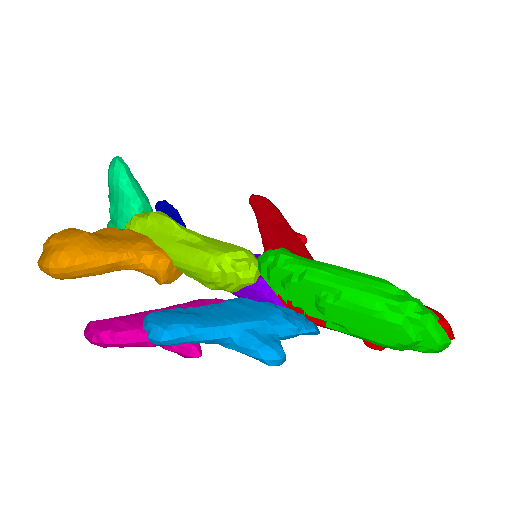
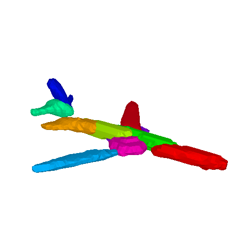
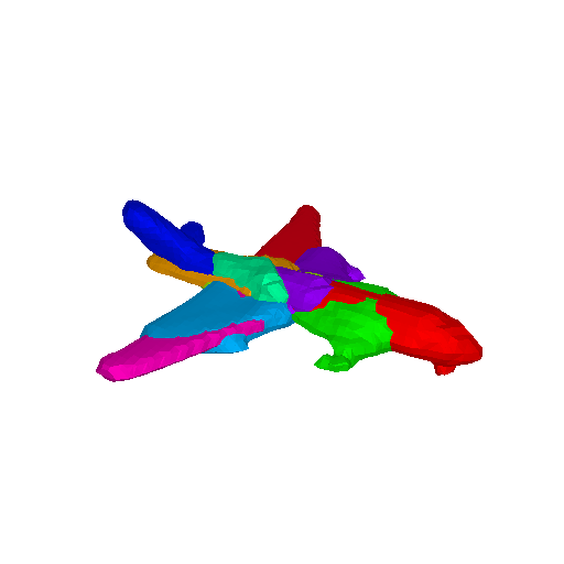
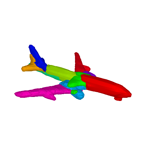
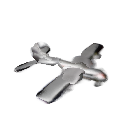
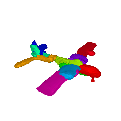
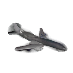
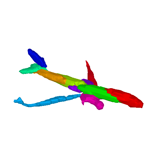
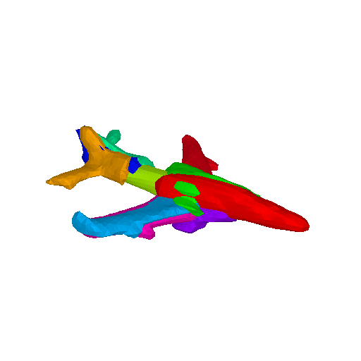
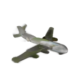
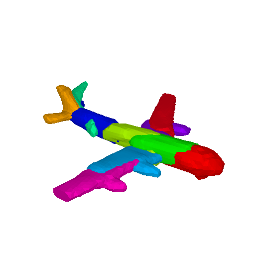
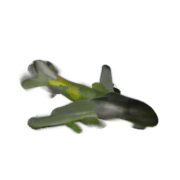
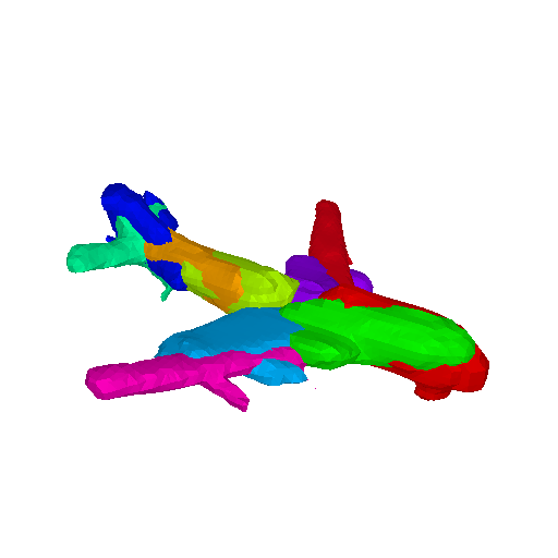
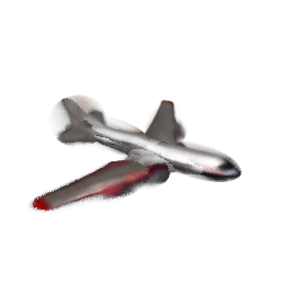
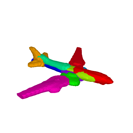
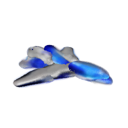
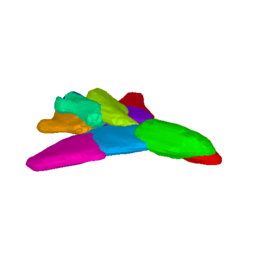
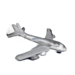
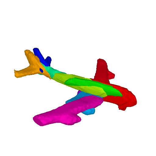
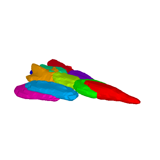
w/o Mask Loss: The mask loss is the squared error between the observed and the rendered pixel value of the object mask for a set of rays. We observe that removing the mask loss $\mathcal{L}_{mask}(\mathcal{R})$ results in more noisy/blurry renderings, in particular around the surface boundaries (see first column in Fig. 17). We experimentally observed that $\mathcal{L}_{mask}(\mathcal{R})$ helps the network find the object boundaries faster, which naturally improves the overall rendering quality. On the part-level, we also observe that the generated parts are less smooth (e.g. see the tail parts of the two last airplanes in the first column of Fig. 17).

w/o Occupancy Loss: The occupancy loss makes sure that the generated shape does not occupy empty space. This is enforced by making sure that the generated parts only contain/cover inside rays, namely rays with $\ell_{r}=1$. Therefore, removing $\mathcal{L}_{occ}(\mathcal{R})$ from our optimization objective results in renderings of worse quality, particularly around the object boundaries (see second column in Fig. 17). Note that in our evaluation, even if we remove this loss, we still use $\mathcal{L}_{mask}(\mathcal{R})$, which forces, to some extent, the network to capture the surface boundary.

w/o Coverage Loss: The coverage loss prevents degenerate parts, that are either too thin or too large. Therefore, when we remove $\mathcal{L}_{cov}(\mathcal{R})$ from our optimization, we note that the generated parts become either very small (first and second example in third column of Fig. 17) or too large (last example in the same column).

w/o Overlapping Loss: The overlapping loss encourages the generated parts to not capture the same regions of the object. We identify overlapping parts by a ray being internal to more than $\lambda$ parts and we set $\lambda=3$. Note that this done using the predicted label for ray $r$ wrt. to part $m$, $\displaystyle\hat{\ell}_{r}^{m}=\max_{\mathbf{x}_{i}^{r}\in\mathcal{X}_{r}}h_{\theta}^{m}(\mathbf{x}_{i}^{r})$. Removing $\mathcal{L}_{overlap}(\mathcal{R})$ results in generated parts that capture the same regions of the object, as shown in the fourth column of Fig. 17.

B.2 Number of Parts

In this section, we analyze the impact of the number of parts on the quality of the generated shapes. Specifically, we train our model with: $5$, $10$, $16$ and $20$ parts. Unlike the results presented in our main submission, for this experiment, we train all model variants on a subset of the Airplanes category, consisting of $178$ training samples, for $50$ epochs. To evaluate the plausibility of the generated shapes, we compute the Minimum Matching Distance (MMD-CD) score between shapes generated with a different number of parts and a set of reference shapes. As reference shapes, we take $10\%$ of the entire test set, which amounts to approximately $46$ shapes. Results are summarized in Tab. 6.

	$5$ Parts	$10$ Parts	$16$ Parts	$20$ Parts
MMD-CD ($\downarrow$)	1.87	1.73	1.53	1.52

Table 6: Ablation Study on the Number of Parts. This table shows a quantitative comparison of our approach with different numbers of parts wrt. MMD-CD ($\downarrow$).

Note that we do not compare our model variants wrt. Coverage (COV), which is a metric indicative of the diversity of the generated shapes, as we only consider a very small reference set of shapes and the results could have been misleading.

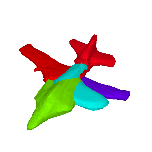
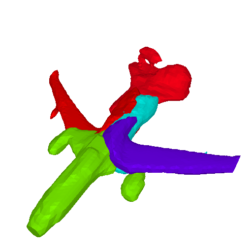
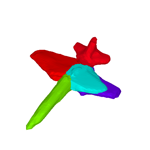
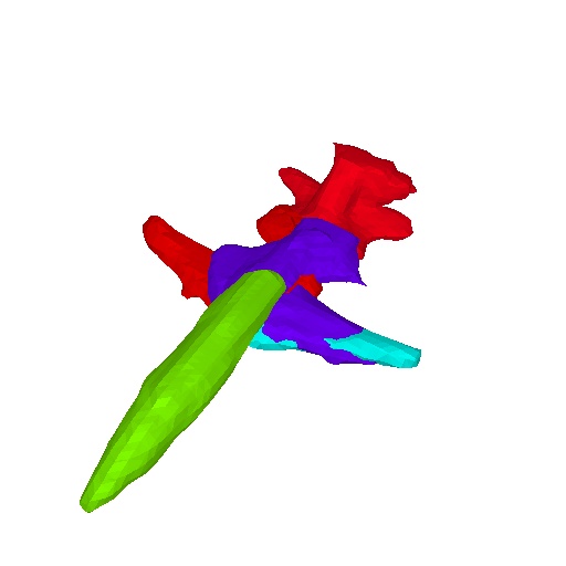
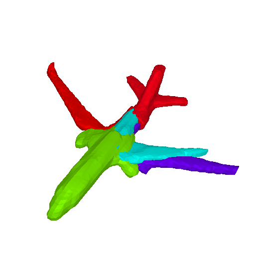
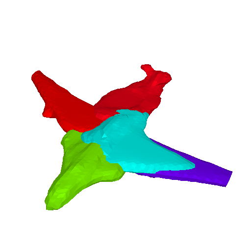
5 Parts

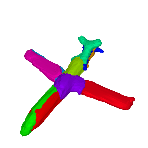
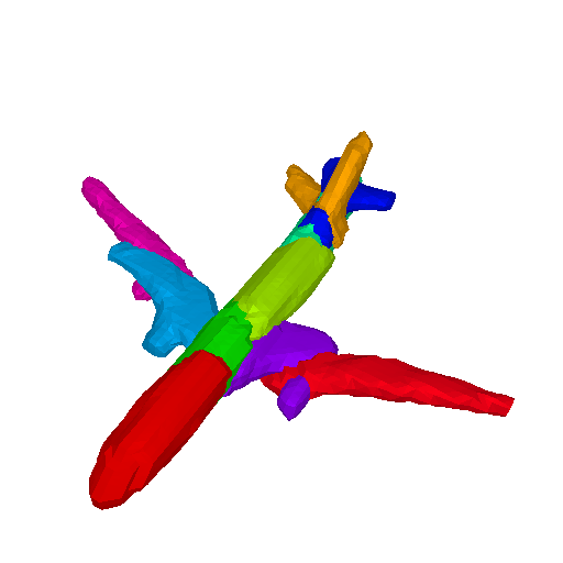
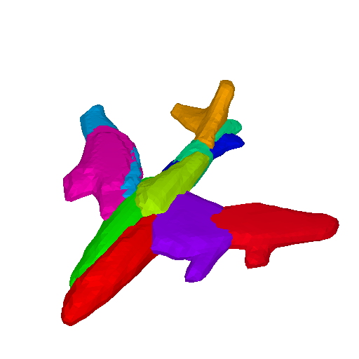
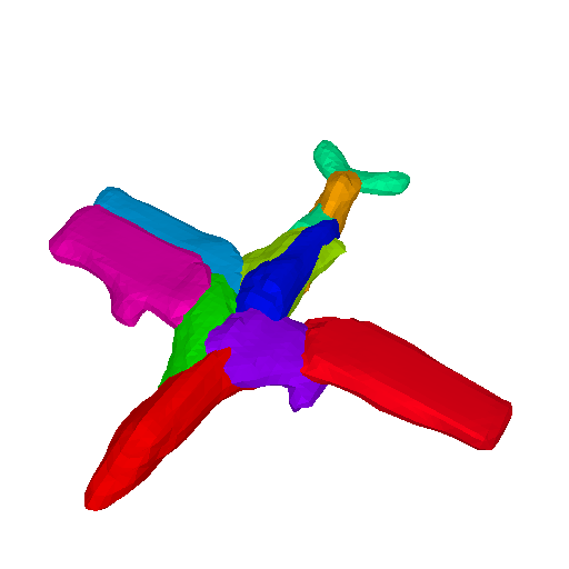
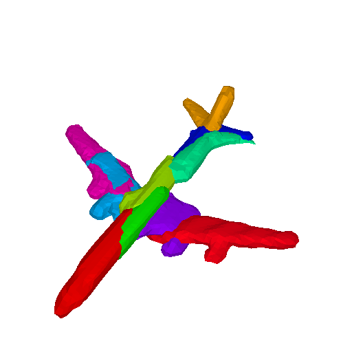
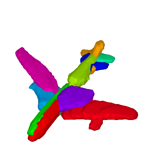
10 Parts

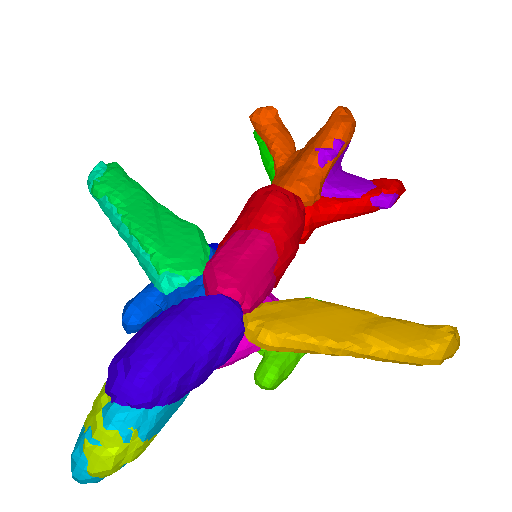
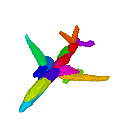
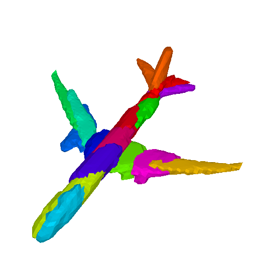
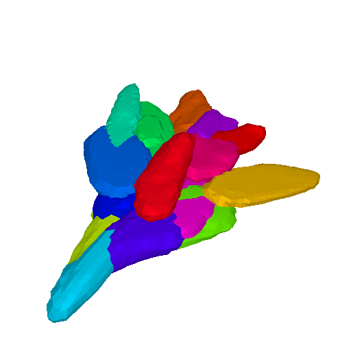
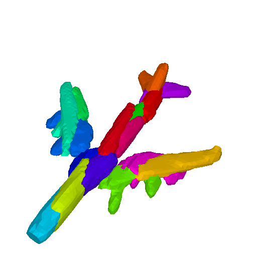
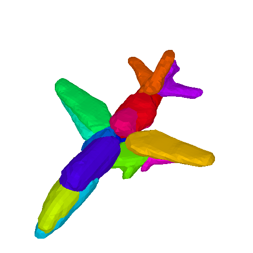
16 Parts

20 Parts

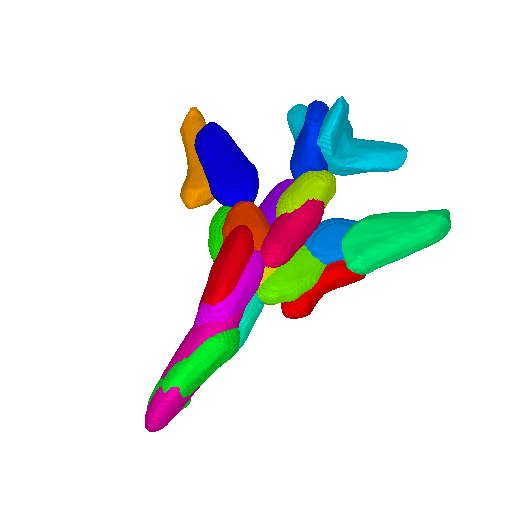
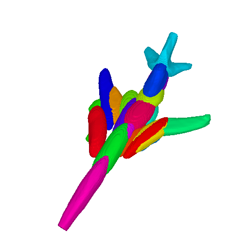
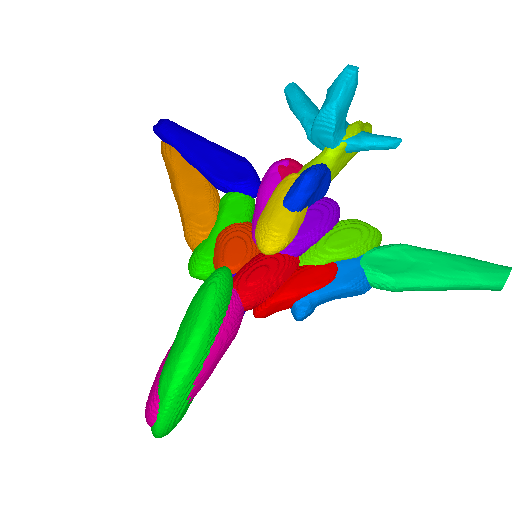
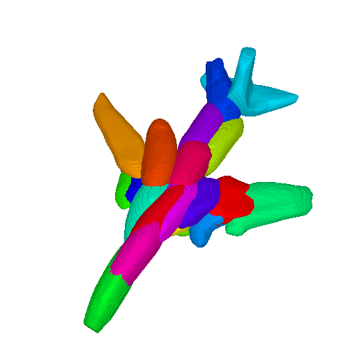
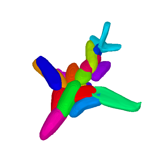
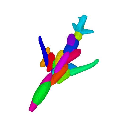
Figure 18: Ablation Study on the Number of Parts. Qualitative evaluation of the impact of the number of parts. The first row shows randomly generated airplanes with $5$ parts, the second row with $10$, the third with $16$, and the last row with $20$ parts. Note that we train a different model for the four different numbers of parts.

From the quantitative comparison in Tab. 6, we observe that the quality of the generated meshes increases for a larger number of parts, namely using more parts yields higher MMD-CD scores. From the qualitative comparison of Fig. 18, we note that using fewer parts results in parts that capture multiple regions of the object, e.g. the red part represents the left wing and the tail. Since our main goal is to enable editability and part-level control, we want to ensure that there is an adequate number of parts so that the user can choose what they want to edit/change. For the case of $10$ parts, we note that now parts are capable of recovering more distinct regions of the object.

B.3 Hard Ray-Part Assignment

In Sec. 4.1 of our main submission, we demonstrate that enabling a soft assignment between parts and rays, namely the color of one ray being determined from multiple parts, prevents several editing operations (see Fig. 5 in our main submission). This is to be expected as for the case of the soft ray-part assignment, the colors and opacities of all rays are determined jointly by all NeRFs. As a result, changing one NeRF naturally affects the others, hence the colors and opacities of parts of the object that we did not intend to change.

Appendix C Additional Experimental Results

In this section, we provide additional information regarding our experiments on ShapeNet [11]. In particular, we consider five categories: Motorbike, Chair, Table, Airplane, Car, which contain 337, 6678, 8509, 4045 and 7497 shapes respectively. For the Car, Table, Airplane and Chair, we use $24$ random views, while for Motorbike we use $100$, as it contains fewer training samples. To ensure fair comparison with our baselines, we use the train-test splits of [27] for the Motorbike, Car, Chair object categories and the train-test splits of [44] for the Airplane, Table category. To render our training data, we randomly sample camera poses from the upper hemisphere of each shape and render images at $256^{2}$ resolution as in [27]. To render both the RGB images and the corresponding object masks we use simple-3dviz[2]. Examples of the rendered RGB images and object masks per category are provided in Fig. 19.

Figure 19: Rendered RGB Images and Object Masks. We provide examples of the rendered RGB images and object masks that we use for training.

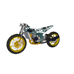
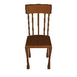
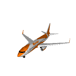
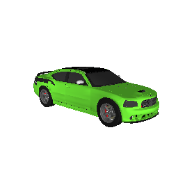
C.1 Shape Generation

In this section, we provide additional qualitative results for our shape generation experiment on the five ShapeNet [11] categories: Motorbike, Chair, Table, Airplane, Car. In particular, we visualize several random samples per category, rendered from a novel view point, not seen during training. In addition, we also show the corresponding 3D meshes and parts. Specifically, in Fig. 20, we illustrate randomly generated motorbikes. We notice that all motorbikes are consistently plausible and the underlying parts meaningfully capture several motorbike’s geometry. Likewise, for the case of generated cars (see Fig. 21) and airplanes (see Fig. 22), we observe that our model is capable of generating diverse geometries and textures that are consistently plausible. For the case of chairs and tables (see Fig. 23), we notice that the geometries are consistently plausible, as also evidenced from Table 1 in our main submission, however the generated textures are less crisp in comparison to the other categories. We hypothesize that this discrepancy stems from the fact that tables and chairs have thinner parts than the other objects. We believe that incorporating a coarse and a fine volume of 3D coordinates would potentially improve this.

Figure 20: Generated Motorbikes. Generated motorbikes accompanied by their corresponding 3D geometries and part-based geometries.

Figure 21: Generated Cars. Generated cars accompanied by their corresponding 3D geometries and part-based geometries.

Figure 22: Generated Airplanes. Generated airplanes accompanied by their corresponding 3D geometries and part-based geometries.

Figure 23: Generated Chairs & Tables. Generated chairs and tables accompanied by their corresponding 3D geometries and part-based geometries.

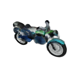
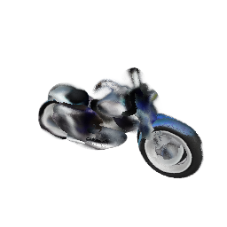
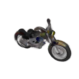
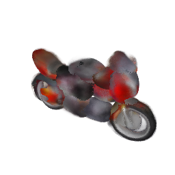
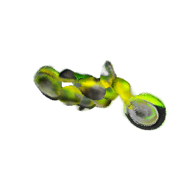
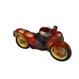
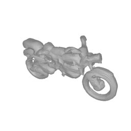
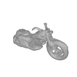
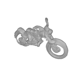
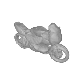
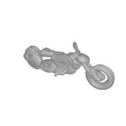
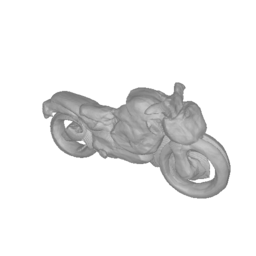
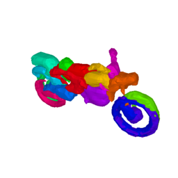
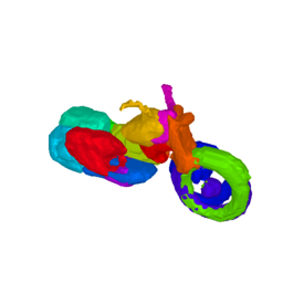
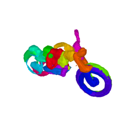
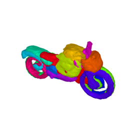
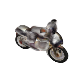
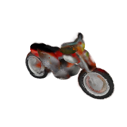
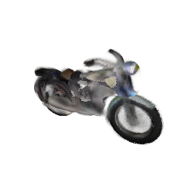
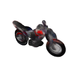
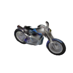
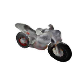
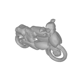
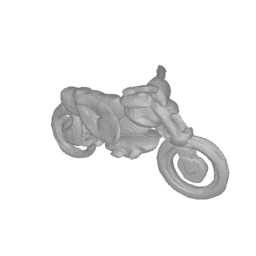
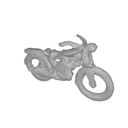
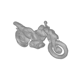
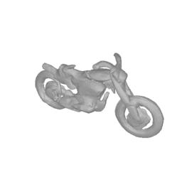
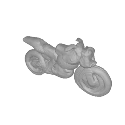
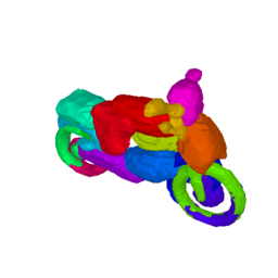
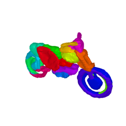
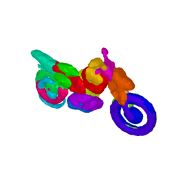
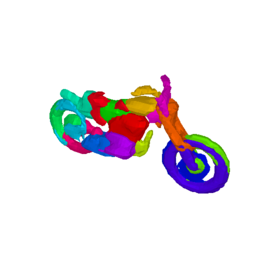
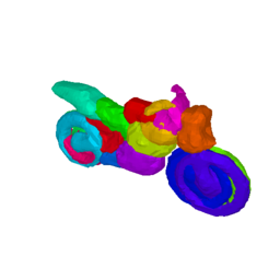
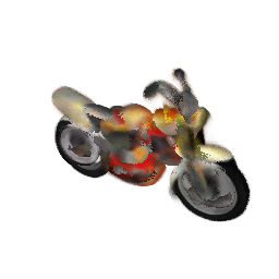
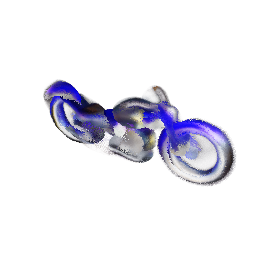
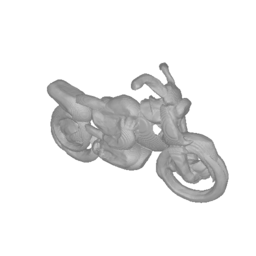
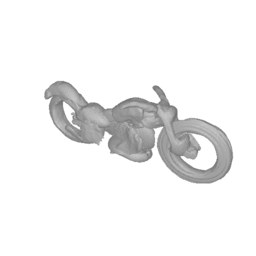
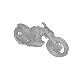
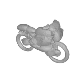
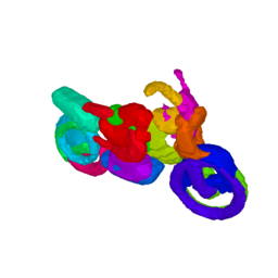
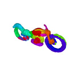
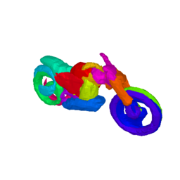
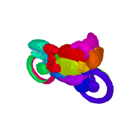
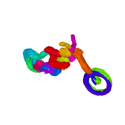
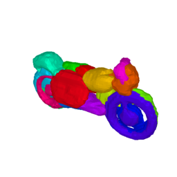
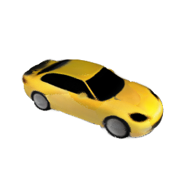
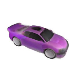
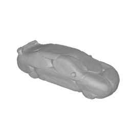
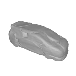
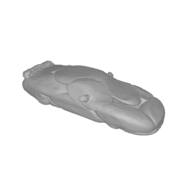
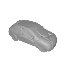
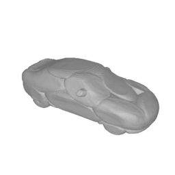
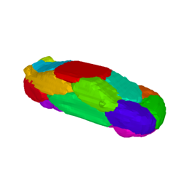
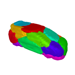
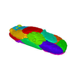
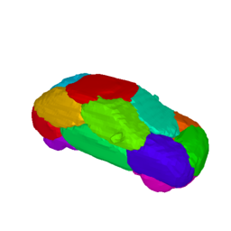
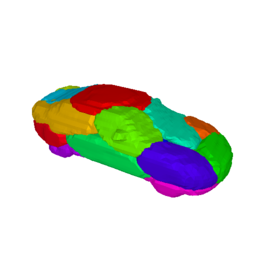
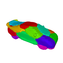
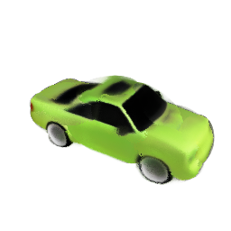
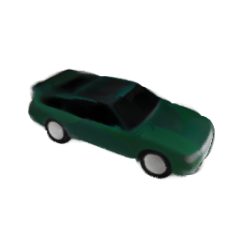
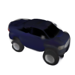
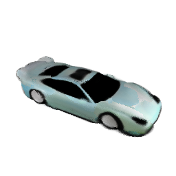
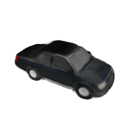
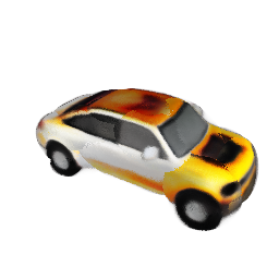
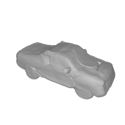
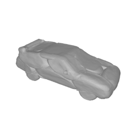
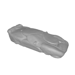
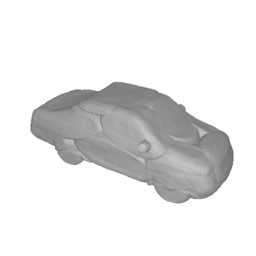
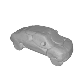
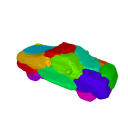
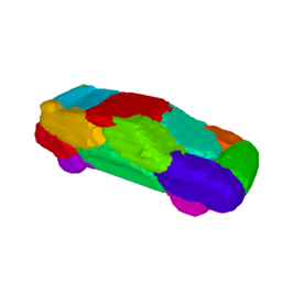
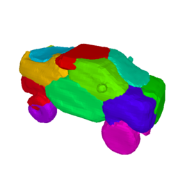
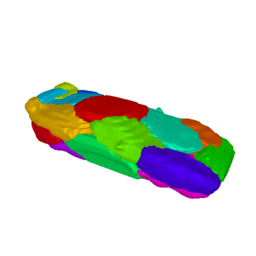
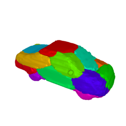
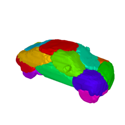
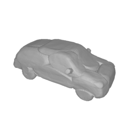
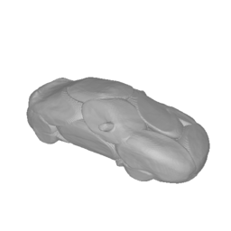
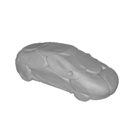
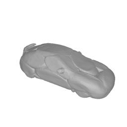
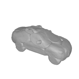
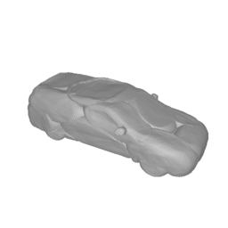
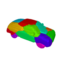
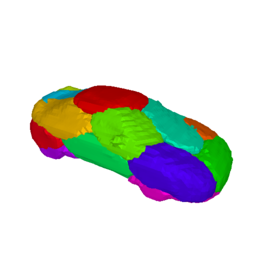
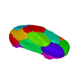
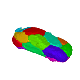
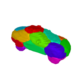
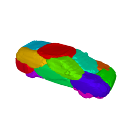
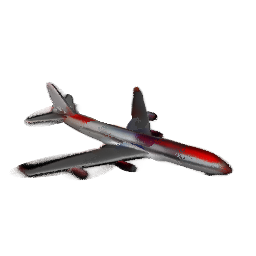
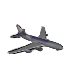
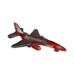
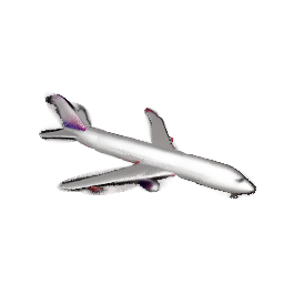
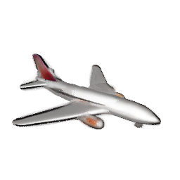
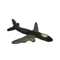
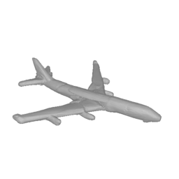
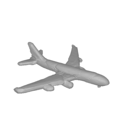
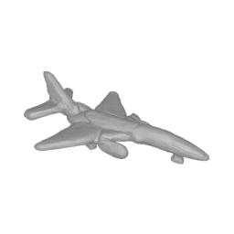
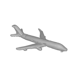
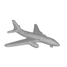
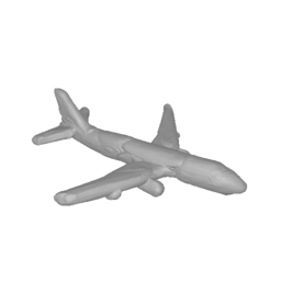
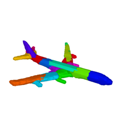
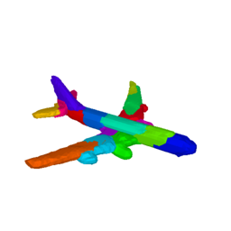
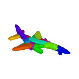
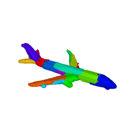
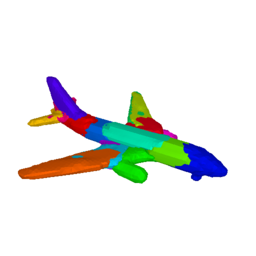
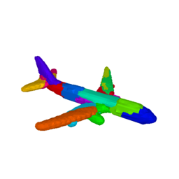
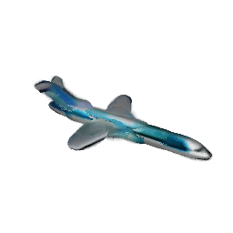
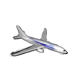
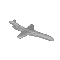
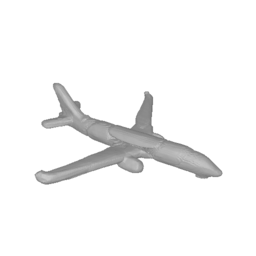
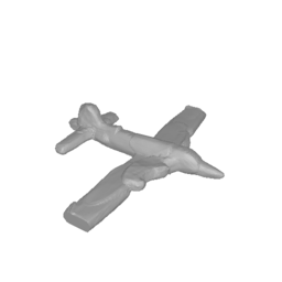
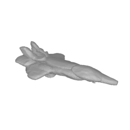
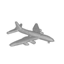
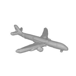
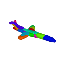
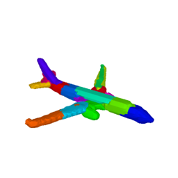
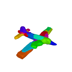
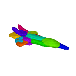
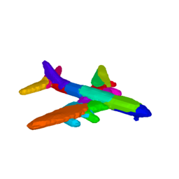
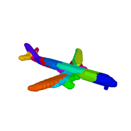
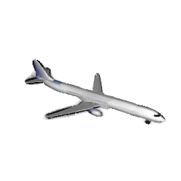
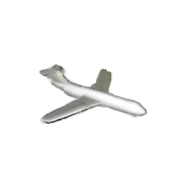
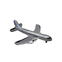
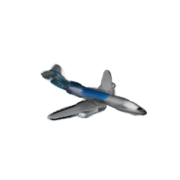
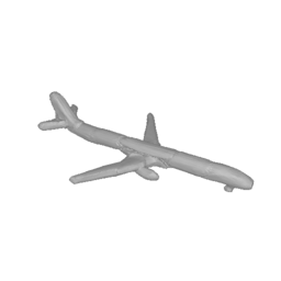
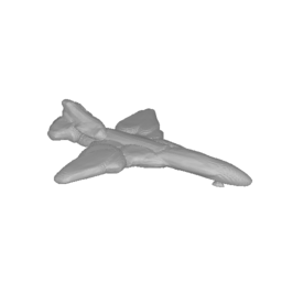
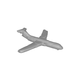
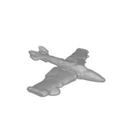
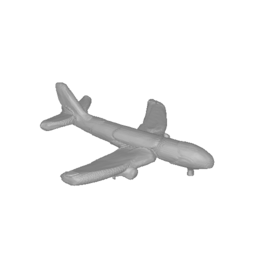
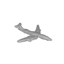
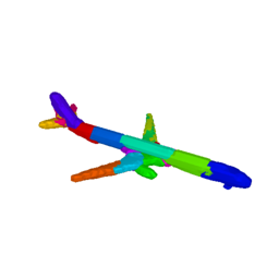
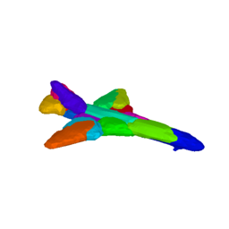
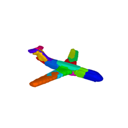
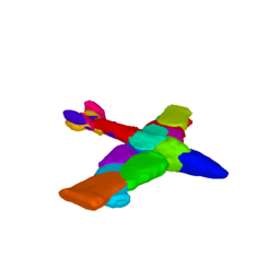
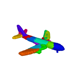
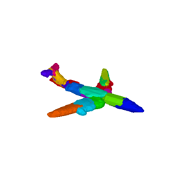
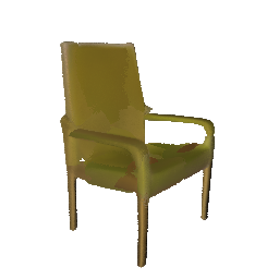
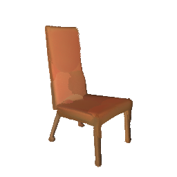
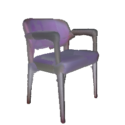
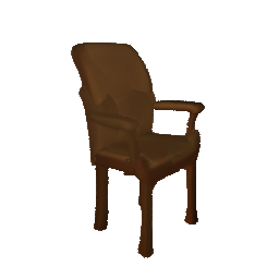
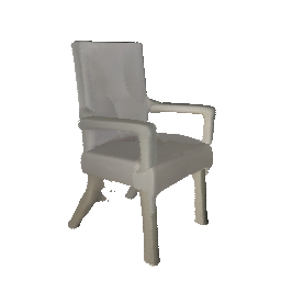
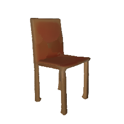
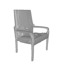
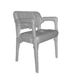
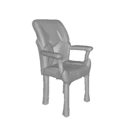
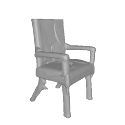
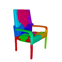
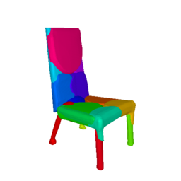
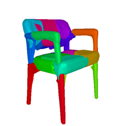
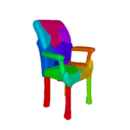
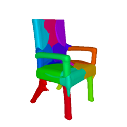
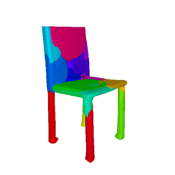
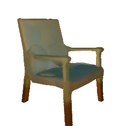
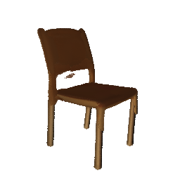
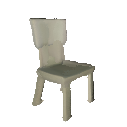
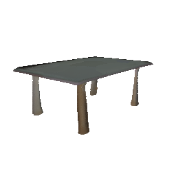
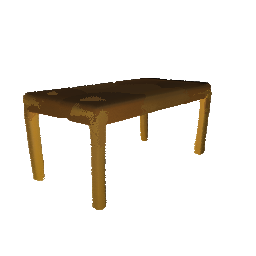
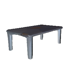
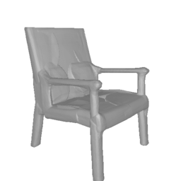
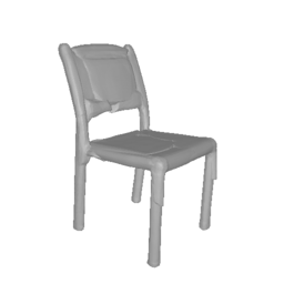
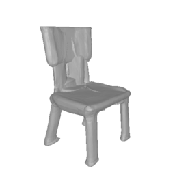
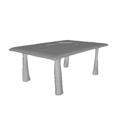
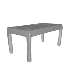
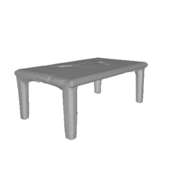
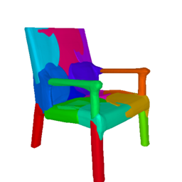
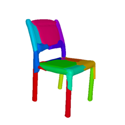
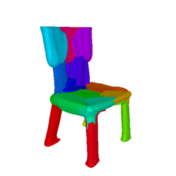
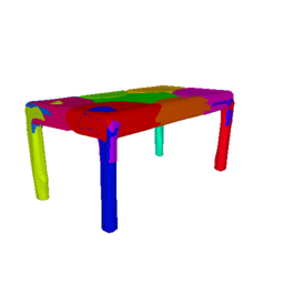
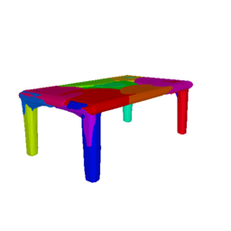
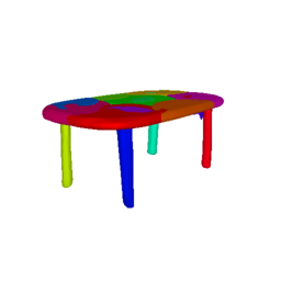
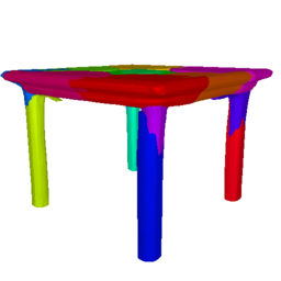
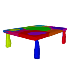
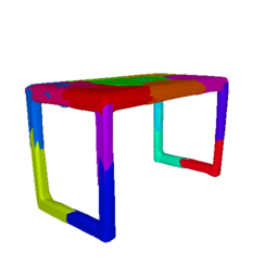
C.1.1 Comparison with Part-Based Generative Models

In this section, we provide more qualitative comparisons of our generated shapes with existing part-based generative methods [44], that require explicit 3D supervision in the form of occupancy labels. In particular, we visualize random samples for three ShapeNet [11] categories: Table, Airplane, Chair. Results are summarized in Fig. 24. Our method can generate geometries of similar quality to [44], without the need of explicit 3D supervision.

SPAGHETTI [44]

Ours

Ours with Parts

SPAGHETTI [44]

Ours

Ours with Parts

SPAGHETTI [44]

Ours

Ours

Figure 24: Shape Generation Comparisons. We compare our model with [44] and show six randomly generated samples per category. The first row per category corresponds to samples from [44], the second row to our results, and the third row to our part geometry results.

C.2 Shape Interpolation

In this section, we show interpolations between the shape and texture codes of two various objects for all object categories. In particular, we interpolate between the latent codes of two shapes and demonstrate that our model is able to smoothly interpolate between two shapes, while preserving the shape structure and the part-based structure for all object categories. Fig. 25 shows three interpolations from left to right between two airplanes. For the case of cars and motorbikes, interpolation results are summarized in Fig. 27 and Fig. 26. Note that for all interpolations the transitions from one shape to the other are consistently meaningful.

Figure 25: Airplanes Shape Interpolation. From left to right, we interpolate between the geometry and texture latent codes of the two airplanes.

Figure 26: Motorbikes Shape Interpolation. From left to right, we interpolate between the geometry and texture latent codes of the two motorbikes.

Figure 27: Cars Shape Interpolation. From left to right, we interpolate between the geometry and texture latent codes of the two cars.

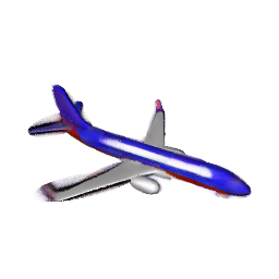
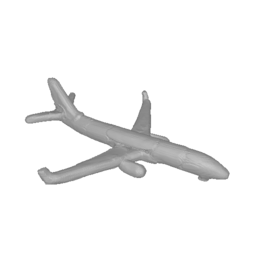
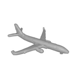
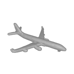
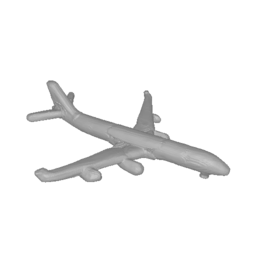
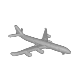
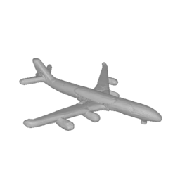
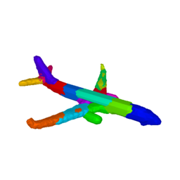
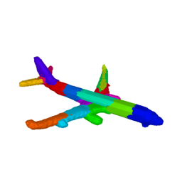
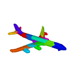
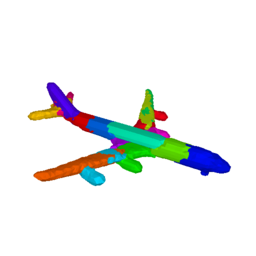
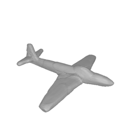
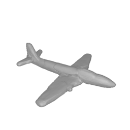
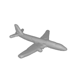
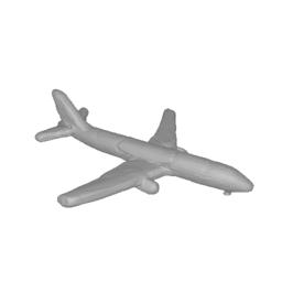
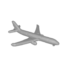
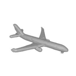
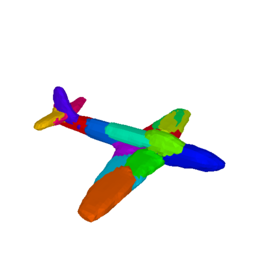
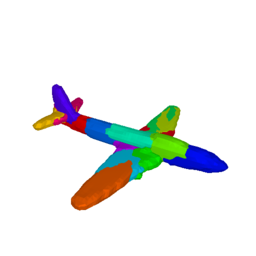
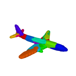
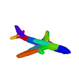
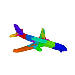
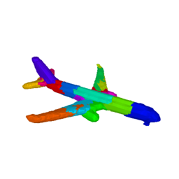
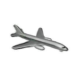
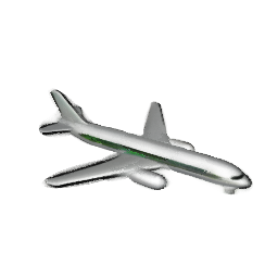
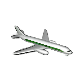
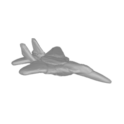
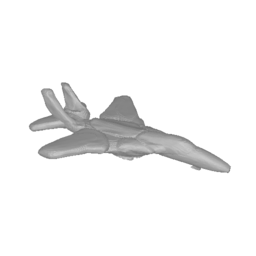
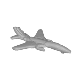
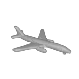
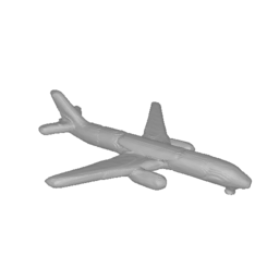
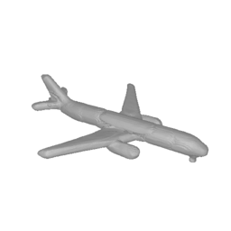
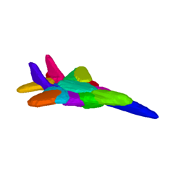
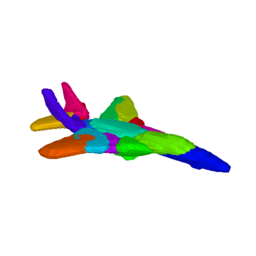
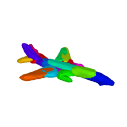
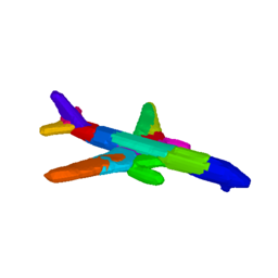
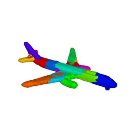
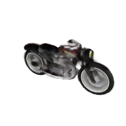
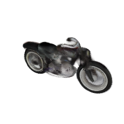
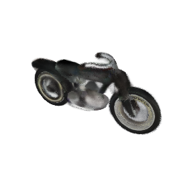
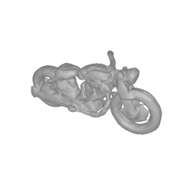
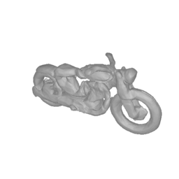
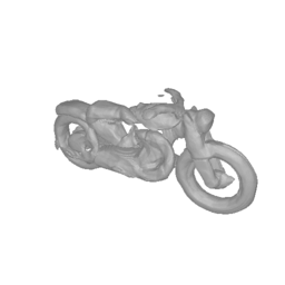
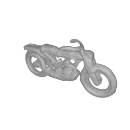
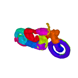
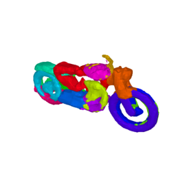
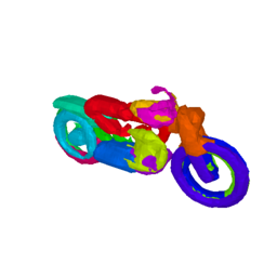
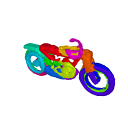
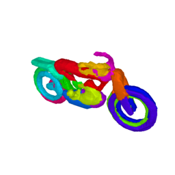
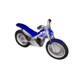
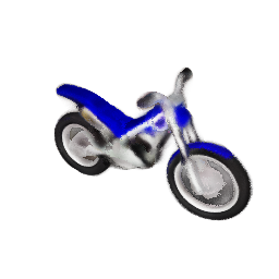
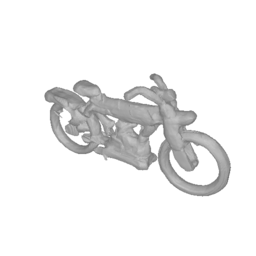
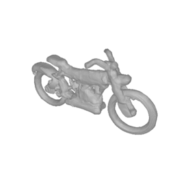
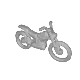
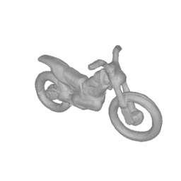
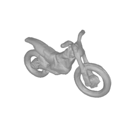
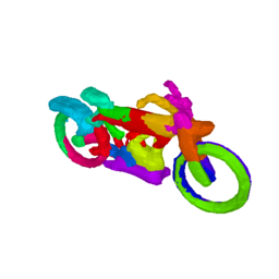
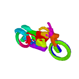
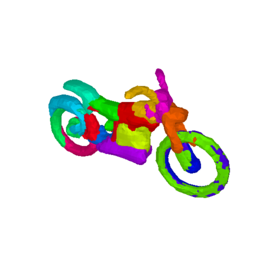
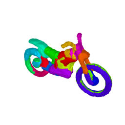
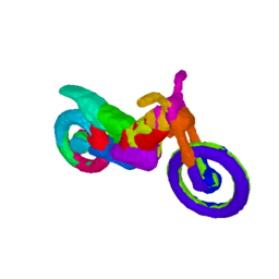
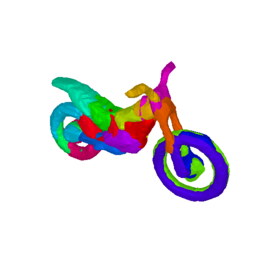
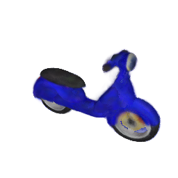
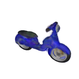
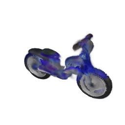
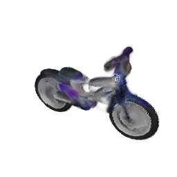
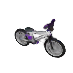
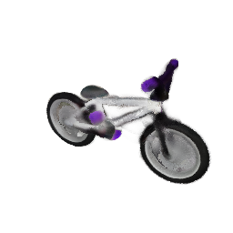
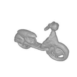
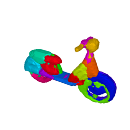
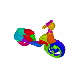
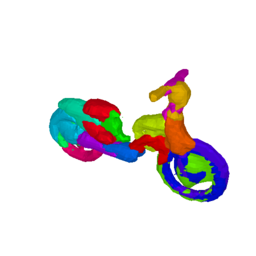
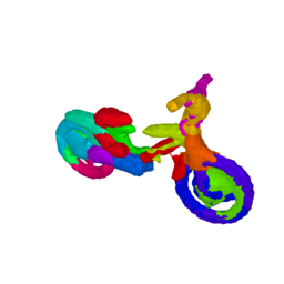
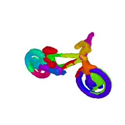
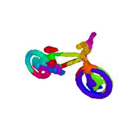
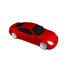
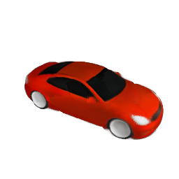
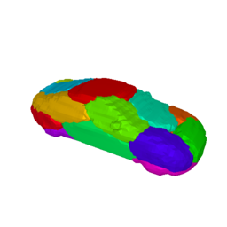
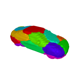
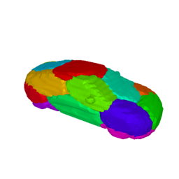
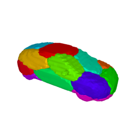
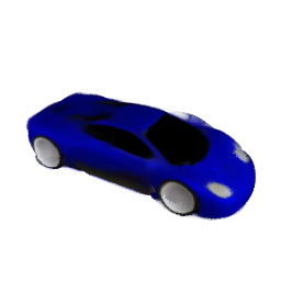
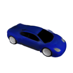
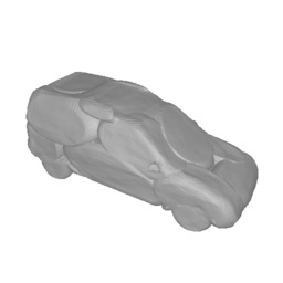
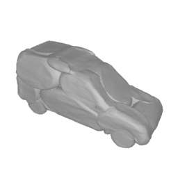
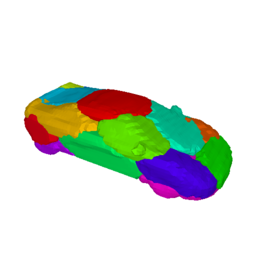
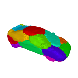
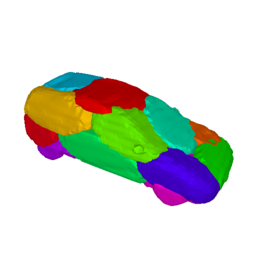
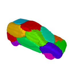
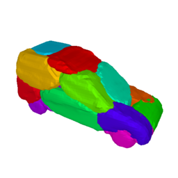
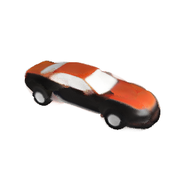
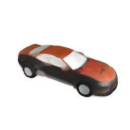
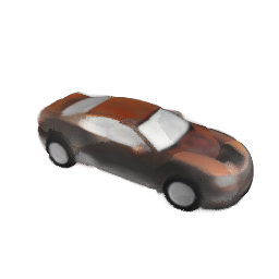
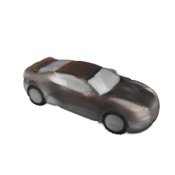
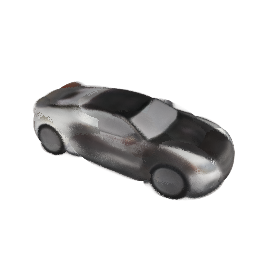
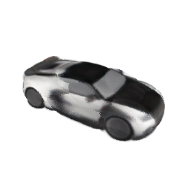
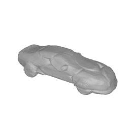
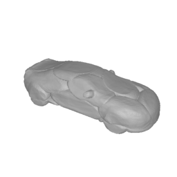
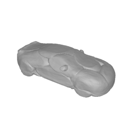
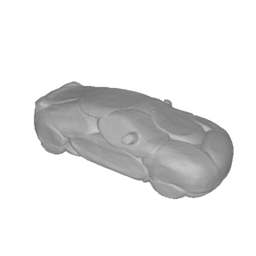
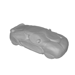
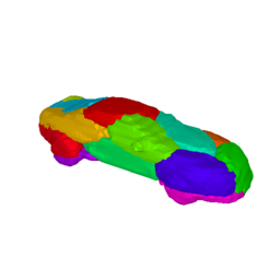
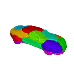
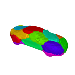
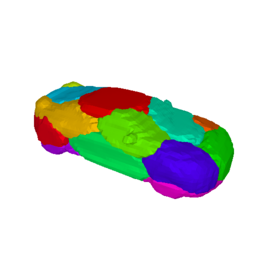
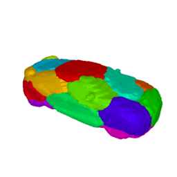
Appendix D Shape Inversion

Our generative model is realized by an auto-decoder architecture. In order to be able to edit a shape that does not belong to the training set, we seek to match the given shape to a shape embedding $\mathbf{z}^{s}$ that can closely reconstruct its geometry. Following [44], we randomly initialize the shape embedding $\mathbf{z}^{s}$, sampling from a multivariate normal distribution using the mean $\boldsymbol{\mu}_{train}^{s}$ and covariance $\boldsymbol{\Sigma}_{train}^{s}$ of shape embeddings seen during training:

$$\mathbf{z}^{s}\sim\mathcal{N}(\boldsymbol{\mu}_{train}^{s},\boldsymbol{\Sigma}_{train}^{s}).$$ (37)

Then, we sample points along rays $\mathcal{R}$ from $N=5$ different views of the object, and freeze our entire network, optimizing the latent code $\mathbf{z}^{s}$ using the following loss function:

$$\mathcal{L}_{inversion}=\mathcal{L}_{mask}(\mathcal{R})+\mathcal{L}_{occ}(\mathcal{R})+\left\|{\mathbf{z}^{s}}\right\|_{2},$$ (38)

using weights 1.0, 1.0 and 0.0001. We optimize the latent code $\mathbf{z}^{s}$ for a fixed number of 700 gradient update steps. Note that this experiment does not require any color information, as we are solely interested in extracting an accurate representation of the geometry of the target shape. We therefore utilize only object masks during optimization. We compare our method with DualSDF [37] and SPAGHETTI [44] on the test set of the ShapeNet Airplanes category. Our results are summarized in Tab. 7. To measure the Chamfer-$L_{1}$ distance, we follow [44] and sample $30,000$ points on the surface of the generated and the target mesh.

	DualSDF	SPAGHETTI	Ours
Chamfer-$L_{1}$	0.806	0.050	0.4536

Table 7: Shape Inversion. Quantitative evaluation of our method against DualSDF [37] and SPAGHETTI [44] wrt. to Chamfer distance ($\downarrow$) on the test set of the Airplanes category.

Ground Truth

Input Object Masks

Ours

Figure 28: Shape Inversion. We show examples of our results when performing shape inversion on the ShapeNet airplanes.

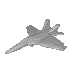
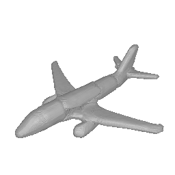
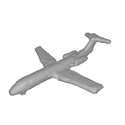
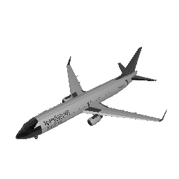
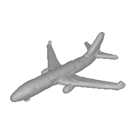
Our model yields better reconstructions than DualSDF [37] in terms of Chamfer distance, even though [37] was trained with explicit 3D supervision. Compared to SPAGHETTI [44], our model yields worse reconstructions. We hypothesize that conditioning our generations to more than $5$ views would further improve the performance of our model. In Fig. 28, we show examples of our shape inversion experiment.

Appendix E Image Inversion

The goal of this experiment is to recover both the appearance and geometry of a 3D shape, as opposed to only the shape as for the case of shape inversion (Sec. D). To this end, we need to find an appropriate match for both the shape and texture embeddings $\{\mathbf{z}^{s},\mathbf{z}^{t}\}$, given a set of posed images and masks as targets. In a similar manner to the sampling process of Sec. A.3, we randomly initialize the shape and texture embeddings, as discussed in Sec. A.3. Then, we freeze the network parameters and optimize the embeddings using the loss function:

$$\mathcal{L}_{image\_inversion}=\mathcal{L}_{rgb}(\mathcal{R})+\mathcal{L}_{mask}(\mathcal{R})+\mathcal{L}_{occ}(\mathcal{R})+\left\|{\mathbf{z}^{s}}\right\|_{2}+\left\|{\mathbf{z}^{t}}\right\|_{2},$$ (39)

with weights of 1.0, 1.0, 1.0, 0.0001 and 0.0001. We use $N=5$ posed images and masks as targets, and optimize the latent codes for a fixed number of 2000 gradient update steps. We showcase several inverted examples in Fig. 29.

Input Images

Ours

Ours - Geometry

Figure 29: Image Inversion. We show examples of our results when performing image inversion on the ShapeNet airplanes.

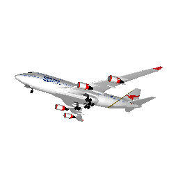
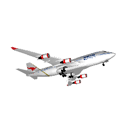
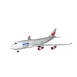
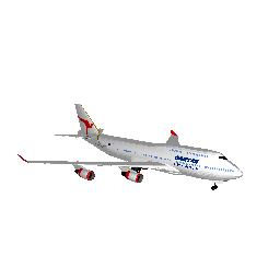
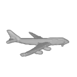
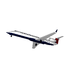
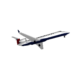
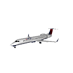
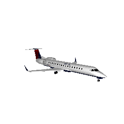
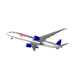
We observe that our model can faithfully recover the object geometry and appearance for various objects. Note that Image Inversion enables users to directly edit shapes, by just providing a few posed images and masks. In Sec. F we showcase several editing functionalities on the inverted shapes.

Appendix F Shape Editing

In this section, we demonstrate the editing capabilities of our model on inverted shapes from ShapeNet Airplane. To perform the image inversion, we follow the process described in Sec. E. In Fig. 30, we show several examples of geometry, texture mixing and shape editing. In particular, we show two shape editing examples, (see last four rows in Fig. 30), where we select several parts from two airplanes and we translate them along the body of the two airplanes. The parts that we select correspond to the tail of the first airplane and the wings of the second, highlighted in green. Across both transformations, only the pose of the selected parts change, while their appearance/texture as well as the shape and appearance of the other parts does not change. For the case of texture mixing (see third and fourth rows in Fig. 30), we start from three airplanes and perform several texture mixing operations. For example, in the last column of the third row of Fig. 30, we show a generated airplane, whose texture and shape for the tail is from the first shape, while the texture and shape for the wings and the body are from the second and third shape respectively. Likewise, for the geometry mixing experiment (see two first rows in Fig. 30), we show examples where we mix the shapes of the three input airplanes, while keeping the texture of the first (fourth column), the second (fifth column) or the third input airplane (sixth column).

Shape 1

Shape 2

Shape 3

Mixing (Texture 1)

Mixing (Texture 2)

Mixing (Texture 3)

Mixing (Combined)

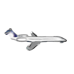
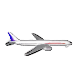
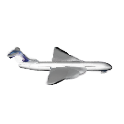
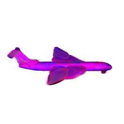
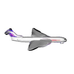
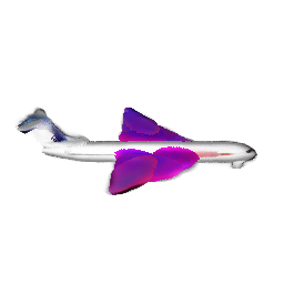
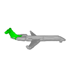
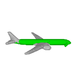
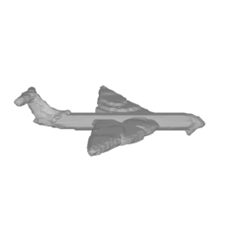
Geometry Mixing

Texture 1

Texture 2

Texture 3

Mixing (Shape 1)

Mixing (Shape 2)

Mixing (Shape 3)

Mixing (Combined)

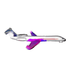
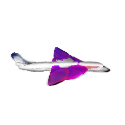
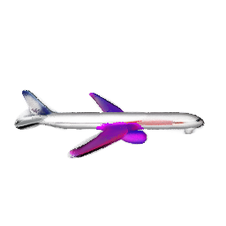
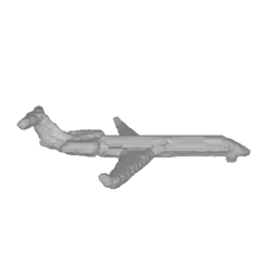
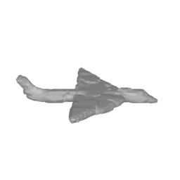
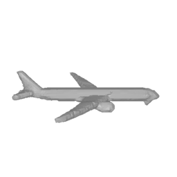
Texture Mixing

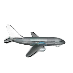
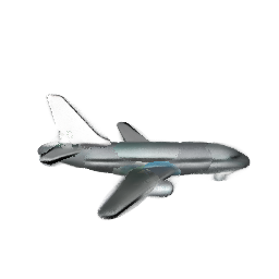
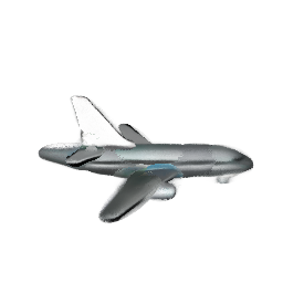
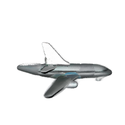
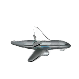
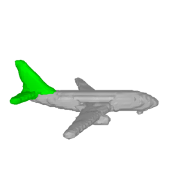
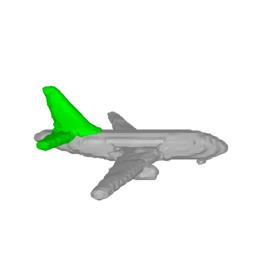
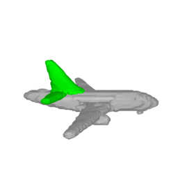
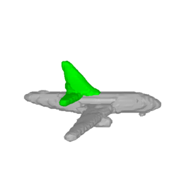
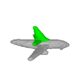
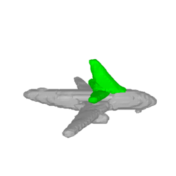
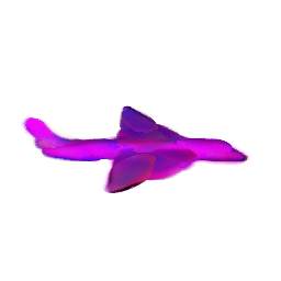
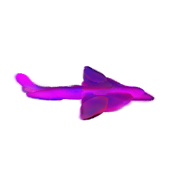
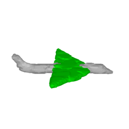
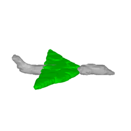
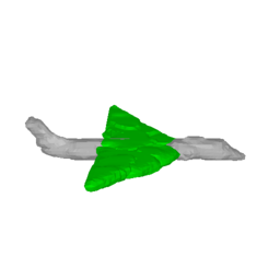
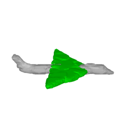
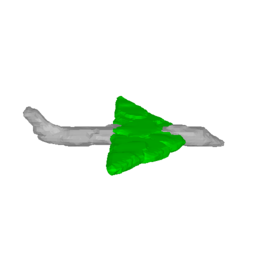
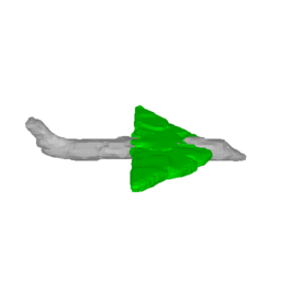
Shape Editing

Figure 30: Shape Editing. We show examples of our results when performing geometry mixing, texture mixing and part editing operations on image inverted ShapeNet airplanes.

Appendix G Discussion and Limitations

In the primitive-based literature, the word part refers to geometric primitives that are typically simple shapes such as cylinders [61], cuboids [116], superquadrics [93, 94], spheres [37] or more generally convex shapes [19]. More recently, the term part has also been used to describe parts that can capture complex geometries and are not limited to simple geometric shapes [31, 92, 56]. Regardless of the part’s expressivity, primitive-based methods yield semantically consistent reconstructions, where the same part is consistently used for representing the same part of the object. Being semantically consistent does not necessarily mean that parts will also be semantically meaningful, namely refer to humanly identifiable parts.

As we parametrize parts by neural radiance fields, our parts can capture complex topologies that are not limited to simple geometric shapes. Examples of our generated parts can be found in Fig. 20$-$Fig. 27. We note that our parts can be coherent across some objects, e.g. the same part is used for representing the same region of the object, in particular when the parts have comparable size and shape. However, for two shapes with different sizes e.g a big and small car (see Fig. 21), we note that our parts are not semantically consistent, namely the part that is used to represent the tire and the top part of the car for a smaller car is now representing only the tire of a bigger car. Note that this is not a limitation only of our work but also of existing part-based methods, as they do not explicitly enforce the semantic consistency of parts.

In addition, in Fig. 31, we provide two examples of the renderings produced using our $16$ NeRFs/parts, when rendering the tractor scene from a novel view and when rendering a ShapeNet car from a novel camera. Although the per-part renderings are consistently crisp and faithfully capture the appearance details of the object, they do not always correspond to semantically meaningful parts. For example, for the case of the tractor scene, our network has associated one part with the bucket of the tractor, however it uses multiple parts to capture regions of the floor, whereas ideally we would like one part to capture the entire floor. Similarly, for the case of the car, while the per-part renderings have sharp colors, they cover parts of the object that are not humanly interpretable, such as a single NeRF representing part of the tire and part of the car.

(a) Tractor Scene

(b) ShapeNet Car

Figure 31: Per-Part Renderings. We show the per-part renderings produced by our $16$ NeRF/parts for a novel view.

This is again a common issue observed in all existing part-based methods [116, 93, 19, 92]. As these methods do not explicitly enforce the meaningfulness of their parts, oftentimes parts are associated with regions of objects that are not meaningful and do not correspond to humanly interpretable parts. We believe that in future research, it would be valuable to explore ways to enforce that parts are more interpretable, in order to unlock more editing operations, that better keep humans in the loop. Our main goal for this work, was to introduce a generative model that enables local control through parts. While increasing the number of parts enables more control on the generated shape, as we can select multiple small parts that compose a semantic part such as the wings of the airplane, we believe that it is useful to also explore other types of more semantic control, where a user for example could select a part based on its semantic class e.g. wing of an airplane or saddle of a motorbike, without having to manually select multiple parts, as is the case for our model.

In contrast to existing NerF-based generative models [105, 10, 9, 26] that rely on adversarial losses to generate high quality renderings, our model does not employ such losses. We believe that incorporating triplane-based representations [9] or adversarial losses could further improve the quality of our generated textures. Moreover, in our current framework, moving one part of an object to a new location outside the object does not necessarily generate a contiguous shape. To address this, [44], introduced a blending network, implemented as a transformer decoder that merges the subsequent parts and synthesizes a novel object. Incorporating such a technique in our model is not possible, as we do not have access to 3D supervision in the form of a mesh. However, we could utilize [134, 65] to synthesize connections between parts.

To summarize, while our work makes an important step towards generating editable 3D shapes, it still has several limitations. In particular, during training, our supervision comes from posed images and object masks. Nevertheless, acquiring detailed masks for objects in the wild is not always possible. Therefore, we believe it would be useful to explore ways to alleviate the need for object masks. Likewise, adopting a formulation like [105] that enables training from unposed images could further extend the capabilities of our model. In addition, while our model can perform several editing operations, our current formulation does not support operations where a part is deformed using techniques such as Neural Cages [133] or Biharmonic Coordinates [121]. Incorporating deformations in our editing operations could unlock several editing applications.

Appendix H Potential Negative Impact on Society

Our proposed model enables generating editable 3D meshes with textures. While, we see this as an important step towards automatic content creation and enabling a multitude of editing functionalities, it can also lead to negative consequences, when applied to sensitive data, such as human bodies or faces. Therefore, we believe it is imperative to always check the license of any 3D publicly available 3D model. In addition, we see the development of techniques for identifying real from synthetic data as an essential research direction that could potential prevent deep fake.

Note that throughout this work, we have only worked with publicly available datasets and did not use any data that involves privacy or copyright concerns. For future users that would like to train our model on new data, we recommend to first remove biases from the training data in order to ensure that our model can fairly capture the diversities in terms of shapes, sizes and textures.

References

- [1] Panos Achlioptas, Olga Diamanti, Ioannis Mitliagkas, and Leonidas J. Guibas. Learning representations and generative models for 3d point clouds. In Proc. of the International Conf. on Machine learning (ICML), 2018.
- [2] Katharopoulos Angelos and Despoina Paschalidou. simple-3dviz. https://simple-3dviz.com, 2020.
- [3] Matan Atzmon, Niv Haim, Lior Yariv, Ofer Israelov, Haggai Maron, and Yaron Lipman. Controlling neural level sets. In Advances in Neural Information Processing Systems (NIPS), 2019.
- [4] Matan Atzmon and Yaron Lipman. SAL: sign agnostic learning of shapes from raw data. In Proc. IEEE Conf. on Computer Vision and Pattern Recognition (CVPR), pages 2562–2571, 2020.
- [5] Sai Bi, Zexiang Xu, Pratul P. Srinivasan, Ben Mildenhall, Kalyan Sunkavalli, Milos Hasan, Yannick Hold-Geoffroy, David J. Kriegman, and Ravi Ramamoorthi. Neural reflectance fields for appearance acquisition. arXiv.org, 2020.
- [6] Piotr Bojanowski, Armand Joulin, David Lopez-Paz, and Arthur Szlam. Optimizing the latent space of generative networks. In Proc. of the International Conf. on Machine learning (ICML), 2018.
- [7] Mark Boss, Raphael Braun, Varun Jampani, Jonathan T. Barron, Ce Liu, and Hendrik P. A. Lensch. Nerd: Neural reflectance decomposition from image collections. In Proc. of the IEEE International Conf. on Computer Vision (ICCV), 2021.
- [8] Andrew Brock, Jeff Donahue, and Karen Simonyan. Large scale GAN training for high fidelity natural image synthesis. In Proc. of the International Conf. on Learning Representations (ICLR), 2019.
- [9] Eric R. Chan, Connor Z. Lin, Matthew A. Chan, Koki Nagano, Boxiao Pan, Shalini De Mello, Orazio Gallo, Leonidas J. Guibas, Jonathan Tremblay, Sameh Khamis, Tero Karras, and Gordon Wetzstein. Efficient geometry-aware 3d generative adversarial networks. In Proc. IEEE Conf. on Computer Vision and Pattern Recognition (CVPR), 2022.
- [10] Eric R. Chan, Marco Monteiro, Petr Kellnhofer, Jiajun Wu, and Gordon Wetzstein. Pi-gan: Periodic implicit generative adversarial networks for 3d-aware image synthesis. In Proc. IEEE Conf. on Computer Vision and Pattern Recognition (CVPR), 2021.
- [11] Angel X. Chang, Thomas A. Funkhouser, Leonidas J. Guibas, Pat Hanrahan, Qi-Xing Huang, Zimo Li, Silvio Savarese, Manolis Savva, Shuran Song, Hao Su, Jianxiong Xiao, Li Yi, and Fisher Yu. Shapenet: An information-rich 3d model repository. arXiv.org, 1512.03012, 2015.
- [12] Hao Chen, Bo He, Hanyu Wang, Yixuan Ren, Ser-Nam Lim, and Abhinav Shrivastava. Nerv: Neural representations for videos. In Advances in Neural Information Processing Systems (NeurIPS), 2021.
- [13] Zhiqin Chen and Hao Zhang. Learning implicit fields for generative shape modeling. In Proc. IEEE Conf. on Computer Vision and Pattern Recognition (CVPR), 2019.
- [14] Zezhou Cheng, Menglei Chai, Jian Ren, Hsin-Ying Lee, Kyle Olszewski, Zeng Huang, Subhransu Maji, and Sergey Tulyakov. Cross-modal 3d shape generation and manipulation. arXiv.org, 2022.
- [15] Julian Chibane, Thiemo Alldieck, and Gerard Pons-Moll. Implicit functions in feature space for 3d shape reconstruction and completion. In Proc. IEEE Conf. on Computer Vision and Pattern Recognition (CVPR), 2020.
- [16] Yunjey Choi, Min-Je Choi, Munyoung Kim, Jung-Woo Ha, Sunghun Kim, and Jaegul Choo. Stargan: Unified generative adversarial networks for multi-domain image-to-image translation. In Proc. IEEE Conf. on Computer Vision and Pattern Recognition (CVPR), 2018.
- [17] Yunjey Choi, Youngjung Uh, Jaejun Yoo, and Jung-Woo Ha. Stargan v2: Diverse image synthesis for multiple domains. In Proc. IEEE Conf. on Computer Vision and Pattern Recognition (CVPR), 2020.
- [18] Harm de Vries, Florian Strub, Jérémie Mary, Hugo Larochelle, Olivier Pietquin, and Aaron C. Courville. Modulating early visual processing by language. In Advances in Neural Information Processing Systems (NIPS), 2017.
- [19] Boyang Deng, Kyle Genova, Soroosh Yazdani, Sofien Bouaziz, Geoffrey Hinton, and Andrea Tagliasacchi. Cvxnets: Learnable convex decomposition. Proc. IEEE Conf. on Computer Vision and Pattern Recognition (CVPR), 2020.
- [20] Yu Deng, Jiaolong Yang, and Xin Tong. Deformed implicit field: Modeling 3d shapes with learned dense correspondence. In Proc. IEEE Conf. on Computer Vision and Pattern Recognition (CVPR), 2021.
- [21] Theo Deprelle, Thibault Groueix, Matthew Fisher, Vladimir G Kim, Bryan C Russell, and Mathieu Aubry. Learning elementary structures for 3d shape generation and matching. In Advances in Neural Information Processing Systems (NIPS), 2019.
- [22] Terrance DeVries, Miguel Ángel Bautista, Nitish Srivastava, Graham W. Taylor, and Joshua M. Susskind. Unconstrained scene generation with locally conditioned radiance fields. In Proc. of the IEEE International Conf. on Computer Vision (ICCV), 2021.
- [23] Tim Elsner, Moritz Ibing, Victor Czech, Julius Nehring-Wirxel, and Leif Kobbelt. Intuitive shape editing in latent space. arXiv.org, 2021.
- [24] Michael S Floater. Mean value coordinates. Computer Aided Geometric Design, 2003.
- [25] Matheus Gadelha, Subhransu Maji, and Rui Wang. 3d shape induction from 2d views of multiple objects. In Proc. of the International Conf. on 3D Vision (3DV), 2017.
- [26] Jun Gao, Wenzheng Chen, Tommy Xiang, Alec Jacobson, Morgan McGuire, and Sanja Fidler. Learning deformable tetrahedral meshes for 3d reconstruction. In Advances in Neural Information Processing Systems (NeurIPS), 2020.
- [27] Jun Gao, Tianchang Shen, Zian Wang, Wenzheng Chen, Kangxue Yin, Daiqing Li, Or Litany, Zan Gojcic, and Sanja Fidler. GET3D: A generative model of high quality 3d textured shapes learned from images. In Advances in Neural Information Processing Systems (NeurIPS), 2022.
- [28] Lin Gao, Jie Yang, Tong Wu, Yu-Jie Yuan, Hongbo Fu, Yu-Kun Lai, and Hao Zhang. SDM-NET: deep generative network for structured deformable mesh. In ACM SIGGRAPH Conference and Exhibition on Computer Graphics and Interactive Techniques in Asia (SIGGRAPH Asia), 2019.
- [29] Stephan J. Garbin, Marek Kowalski, Matthew Johnson, Jamie Shotton, and Julien P. C. Valentin. Fastnerf: High-fidelity neural rendering at 200fps. In Proc. of the IEEE International Conf. on Computer Vision (ICCV), 2021.
- [30] Kyle Genova, Forrester Cole, Avneesh Sud, Aaron Sarna, and Thomas A. Funkhouser. Local deep implicit functions for 3d shape. In Proc. IEEE Conf. on Computer Vision and Pattern Recognition (CVPR), 2020.
- [31] Kyle Genova, Forrester Cole, Avneesh Sud, Aaron Sarna, and Thomas A. Funkhouser. Local deep implicit functions for 3d shape. In Proc. IEEE Conf. on Computer Vision and Pattern Recognition (CVPR), 2020.
- [32] Kyle Genova, Forrester Cole, Daniel Vlasic, Aaron Sarna, William T Freeman, and Thomas Funkhouser. Learning shape templates with structured implicit functions. In Proc. of the IEEE International Conf. on Computer Vision (ICCV), 2019.
- [33] Ian J. Goodfellow, Jean Pouget-Abadie, Mehdi Mirza, Bing Xu, David Warde-Farley, Sherjil Ozair, Aaron C. Courville, and Yoshua Bengio. Generative adversarial nets. In Advances in Neural Information Processing Systems (NIPS), 2014.
- [34] Amos Gropp, Lior Yariv, Niv Haim, Matan Atzmon, and Yaron Lipman. Implicit geometric regularization for learning shapes. In Proc. of the International Conf. on Machine learning (ICML), 2020.
- [35] Jiatao Gu, Lingjie Liu, Peng Wang, and Christian Theobalt. Stylenerf: A style-based 3d aware generator for high-resolution image synthesis. In Proc. of the International Conf. on Learning Representations (ICLR), 2022.
- [36] William Rowan Hamilton. Xi. on quaternions; or on a new system of imaginaries in algebra. The London, Edinburgh, and Dublin Philosophical Magazine and Journal of Science, 33(219):58–60, 1848.
- [37] Zekun Hao, Hadar Averbuch-Elor, Noah Snavely, and Serge J. Belongie. Dualsdf: Semantic shape manipulation using a two-level representation. In Proc. IEEE Conf. on Computer Vision and Pattern Recognition (CVPR), 2020.
- [38] Zekun Hao, Arun Mallya, Serge J. Belongie, and Ming-Yu Liu. Gancraft: Unsupervised 3d neural rendering of minecraft worlds. In Proc. of the IEEE International Conf. on Computer Vision (ICCV), 2021.
- [39] Kaiming He, Xiangyu Zhang, Shaoqing Ren, and Jian Sun. Deep residual learning for image recognition. In Proc. IEEE Conf. on Computer Vision and Pattern Recognition (CVPR), 2016.
- [40] Paul Henderson and Vittorio Ferrari. Learning single-image 3d reconstruction by generative modelling of shape, pose and shading. International Journal of Computer Vision (IJCV), 2019.
- [41] Paul Henderson and Christoph H. Lampert. Unsupervised object-centric video generation and decomposition in 3d. In Advances in Neural Information Processing Systems (NeurIPS), 2020.
- [42] Philipp Henzler, Niloy J Mitra, , and Tobias Ritschel. Escaping plato’s cave: 3d shape from adversarial rendering. In Proc. of the IEEE International Conf. on Computer Vision (ICCV), 2019.
- [43] Philipp Henzler, Jeremy Reizenstein, Patrick Labatut, Roman Shapovalov, Tobias Ritschel, Andrea Vedaldi, and David Novotný. Unsupervised learning of 3d object categories from videos in the wild. In Proc. IEEE Conf. on Computer Vision and Pattern Recognition (CVPR), 2021.
- [44] Amir Hertz, Or Perel, Raja Giryes, Olga Sorkine-Hornung, and Daniel Cohen-Or. SPAGHETTI: editing implicit shapes through part aware generation. ACM Trans. on Graphics, 2022.
- [45] Amir Hertz, Or Perel, Raja Giryes, Olga Sorkine-Hornung, and Daniel Cohen-Or. Spaghetti: Editing implicit shapes through part aware generation. arXiv.org, 2022.
- [46] Phillip Isola, Jun-Yan Zhu, Tinghui Zhou, and Alexei A. Efros. Image-to-image translation with conditional adversarial networks. In Proc. IEEE Conf. on Computer Vision and Pattern Recognition (CVPR), 2017.
- [47] Wonbong Jang and Lourdes Agapito. Codenerf: Disentangled neural radiance fields for object categories. In Proc. of the IEEE International Conf. on Computer Vision (ICCV), 2021.
- [48] Chiyu Jiang, Avneesh Sud, Ameesh Makadia, Jingwei Huang, Matthias Nießner, and Thomas Funkhouser. Local implicit grid representations for 3d scenes. In Proc. IEEE Conf. on Computer Vision and Pattern Recognition (CVPR), 2020.
- [49] Pushkar Joshi, Mark Meyer, Tony DeRose, Brian Green, and Tom Sanocki. Harmonic coordinates for character articulation. ACM Trans. on Graphics, 2007.
- [50] James T. Kajiya and Brian Von Herzen. Ray tracing volume densities. In ACM Trans. on Graphics, 1984.
- [51] Kacper Kania, Kwang Moo Yi, Marek Kowalski, Tomasz Trzciński, and Andrea Tagliasacchi. Conerf: Controllable neural radiance fields. In Proc. IEEE Conf. on Computer Vision and Pattern Recognition (CVPR), 2022.
- [52] Tero Karras, Timo Aila, Samuli Laine, and Jaakko Lehtinen. Progressive growing of GANs for improved quality, stability, and variation. In Proc. of the International Conf. on Learning Representations (ICLR), 2018.
- [53] Tero Karras, Miika Aittala, Samuli Laine, Erik Härkönen, Janne Hellsten, Jaakko Lehtinen, and Timo Aila. Alias-free generative adversarial networks. In Advances in Neural Information Processing Systems (NeurIPS), 2021.
- [54] Tero Karras, Samuli Laine, Miika Aittala, Janne Hellsten, Jaakko Lehtinen, and Timo Aila. Analyzing and improving the image quality of StyleGAN. 2020.
- [55] Yuki Kawana, Yusuke Mukuta, and Tatsuya Harada. Neural star domain as primitive representation. In Advances in Neural Information Processing Systems (NIPS), 2020.
- [56] Yuki Kawana, Yusuke Mukuta, and Tatsuya Harada. Neural star domain as primitive representation. arXiv.org, 2020.
- [57] Diederik P. Kingma and Jimmy Ba. Adam: A method for stochastic optimization. In Proc. of the International Conf. on Learning Representations (ICLR), 2015.
- [58] Samuli Laine, Janne Hellsten, Tero Karras, Yeongho Seol, Jaakko Lehtinen, and Timo Aila. Modular primitives for high-performance differentiable rendering. ACM Trans. on Graphics, 2020.
- [59] Verica Lazova, Vladimir Guzov, Kyle Olszewski, Sergey Tulyakov, and Gerard Pons-Moll. Control-nerf: Editable feature volumes for scene rendering and manipulation. arXiv.org, 2022.
- [60] Jun Li, Kai Xu, Siddhartha Chaudhuri, Ersin Yumer, Hao (Richard) Zhang, and Leonidas J. Guibas. GRASS: generative recursive autoencoders for shape structures. ACM Trans. on Graphics, 36(4), 2017.
- [61] Lingxiao Li, Minhyuk Sung, Anastasia Dubrovina, Li Yi, and Leonidas Guibas. Supervised fitting of geometric primitives to 3d point clouds. In Proc. IEEE Conf. on Computer Vision and Pattern Recognition (CVPR), 2019.
- [62] Ruihui Li, Xianzhi Li, Ka-Hei Hui, and Chi-Wing Fu. SP-GAN: sphere-guided 3d shape generation and manipulation. ACM Trans. on Graphics, 2021.
- [63] Yichen Li, Kaichun Mo, Lin Shao, Minhyuk Sung, and Leonidas J. Guibas. Learning 3d part assembly from a single image. In Proc. of the European Conf. on Computer Vision (ECCV), 2020.
- [64] Yiyi Liao, Katja Schwarz, Lars M. Mescheder, and Andreas Geiger. Towards unsupervised learning of generative models for 3d controllable image synthesis. Proc. IEEE Conf. on Computer Vision and Pattern Recognition (CVPR), 2020.
- [65] Connor Z. Lin, Niloy J. Mitra, Gordon Wetzstein, Leonidas J. Guibas, and Paul Guerrero. Neuform: Adaptive overfitting for neural shape editing. In Advances in Neural Information Processing Systems (NeurIPS), 2022.
- [66] David B. Lindell, Julien N. P. Martel, and Gordon Wetzstein. Autoint: Automatic integration for fast neural volume rendering. In Proc. IEEE Conf. on Computer Vision and Pattern Recognition (CVPR), 2021.
- [67] Yaron Lipman, David Levin, and Daniel Cohen-Or. Green coordinates. ACM Trans. on Graphics, 2008.
- [68] Lingjie Liu, Jiatao Gu, Kyaw Zaw Lin, Tat-Seng Chua, and Christian Theobalt. Neural sparse voxel fields. In Advances in Neural Information Processing Systems (NeurIPS), 2020.
- [69] Steven Liu, Xiuming Zhang, Zhoutong Zhang, Richard Zhang, Jun-Yan Zhu, and Bryan Russell. Editing conditional radiance fields. In Proc. of the IEEE International Conf. on Computer Vision (ICCV), 2021.
- [70] William E. Lorensen and Harvey E. Cline. Marching cubes: A high resolution 3d surface construction algorithm. In ACM Trans. on Graphics, 1987.
- [71] Sebastian Lunz, Yingzhen Li, Andrew W. Fitzgibbon, and Nate Kushman. Inverse graphics gan: Learning to generate 3d shapes from unstructured 2d data. arXiv.org, 2020.
- [72] Ricardo Martin-Brualla, Noha Radwan, Mehdi S. M. Sajjadi, Jonathan T. Barron, Alexey Dosovitskiy, and Daniel Duckworth. Nerf in the wild: Neural radiance fields for unconstrained photo collections. In Proc. IEEE Conf. on Computer Vision and Pattern Recognition (CVPR), 2021.
- [73] Quan Meng, Anpei Chen, Haimin Luo, Minye Wu, Hao Su, Lan Xu, Xuming He, and Jingyi Yu. Gnerf: Gan-based neural radiance field without posed camera. In Proc. of the IEEE International Conf. on Computer Vision (ICCV), 2021.
- [74] Lars Mescheder, Michael Oechsle, Michael Niemeyer, Sebastian Nowozin, and Andreas Geiger. Occupancy networks: Learning 3d reconstruction in function space. In Proc. IEEE Conf. on Computer Vision and Pattern Recognition (CVPR), 2019.
- [75] Mateusz Michalkiewicz, Jhony K Pontes, Dominic Jack, Mahsa Baktashmotlagh, and Anders Eriksson. Implicit surface representations as layers in neural networks. In Proc. of the IEEE International Conf. on Computer Vision (ICCV), 2019.
- [76] Ben Mildenhall, Pratul P Srinivasan, Matthew Tancik, Jonathan T Barron, Ravi Ramamoorthi, and Ren Ng. NeRF: Representing scenes as neural radiance fields for view synthesis. In Proc. of the European Conf. on Computer Vision (ECCV), 2020.
- [77] Kaichun Mo, Paul Guerrero, Li Yi, Hao Su, Peter Wonka, Niloy Mitra, and Leonidas Guibas. Structurenet: Hierarchical graph networks for 3d shape generation. In ACM Trans. on Graphics, 2019.
- [78] Kaichun Mo, Paul Guerrero, Li Yi, Hao Su, Peter Wonka, Niloy J. Mitra, and Leonidas J. Guibas. Structedit: Learning structural shape variations. In Proc. IEEE Conf. on Computer Vision and Pattern Recognition (CVPR), 2020.
- [79] Thomas Müller, Alex Evans, Christoph Schied, and Alexander Keller. Instant neural graphics primitives with a multiresolution hash encoding. ACM Trans. on Graphics, 2022.
- [80] Thu Nguyen-Phuoc, Chuan Li, Lucas Theis, Christian Richardt, and Yong-Liang Yang. Hologan: Unsupervised learning of 3d representations from natural images. In Proc. of the IEEE International Conf. on Computer Vision (ICCV), 2019.
- [81] Thu Nguyen-Phuoc, Chuan Li, Lucas Theis, Christian Richardt, and Yong-Liang Yang. Hologan: Unsupervised learning of 3d representations from natural images. In Proc. of the IEEE International Conf. on Computer Vision (ICCV), 2019.
- [82] Thu Nguyen-Phuoc, Christian Richardt, Long Mai, Yong-Liang Yang, and Niloy Mitra. Blockgan: Learning 3d object-aware scene representations from unlabelled images. arXiv.org, 2020.
- [83] Thu Nguyen-Phuoc, Christian Richardt, Long Mai, Yong-Liang Yang, and Niloy J. Mitra. Blockgan: Learning 3d object-aware scene representations from unlabelled images. In Advances in Neural Information Processing Systems (NeurIPS), 2020.
- [84] Michael Niemeyer and Andreas Geiger. CAMPARI: camera-aware decomposed generative neural radiance fields. In Proc. of the International Conf. on 3D Vision (3DV), 2021.
- [85] Michael Niemeyer and Andreas Geiger. Giraffe: Representing scenes as compositional generative neural feature fields. In Proc. IEEE Conf. on Computer Vision and Pattern Recognition (CVPR), 2021.
- [86] Michael Niemeyer, Lars Mescheder, Michael Oechsle, and Andreas Geiger. Differentiable volumetric rendering: Learning implicit 3d representations without 3d supervision. In Proc. IEEE Conf. on Computer Vision and Pattern Recognition (CVPR), 2020.
- [87] Chengjie Niu, Jun Li, and Kai Xu. Im2struct: Recovering 3d shape structure from a single RGB image. In Proc. IEEE Conf. on Computer Vision and Pattern Recognition (CVPR), 2018.
- [88] Atsuhiro Noguchi, Umar Iqbal, Jonathan Tremblay, Tatsuya Harada, and Orazio Gallo. Watch it move: Unsupervised discovery of 3d joints for re-posing of articulated objects. In Proc. IEEE Conf. on Computer Vision and Pattern Recognition (CVPR), 2022.
- [89] Michael Oechsle, Michael Niemeyer, Christian Reiser, Lars Mescheder, Thilo Strauss, and Andreas Geiger. Learning implicit surface light fields. In Proc. of the International Conf. on 3D Vision (3DV), 2020.
- [90] Michael Oechsle, Songyou Peng, and Andreas Geiger. UNISURF: unifying neural implicit surfaces and radiance fields for multi-view reconstruction. In Proc. of the IEEE International Conf. on Computer Vision (ICCV), 2021.
- [91] Jeong Joon Park, Peter Florence, Julian Straub, Richard A. Newcombe, and Steven Lovegrove. Deepsdf: Learning continuous signed distance functions for shape representation. In Proc. IEEE Conf. on Computer Vision and Pattern Recognition (CVPR), 2019.
- [92] Despoina Paschalidou, Angelos Katharopoulos, Andreas Geiger, and Sanja Fidler. Neural parts: Learning expressive 3d shape abstractions with invertible neural networks. In Proc. IEEE Conf. on Computer Vision and Pattern Recognition (CVPR), 2021.
- [93] Despoina Paschalidou, Ali Osman Ulusoy, and Andreas Geiger. Superquadrics revisited: Learning 3d shape parsing beyond cuboids. In Proc. IEEE Conf. on Computer Vision and Pattern Recognition (CVPR), 2019.
- [94] Despoina Paschalidou, Luc van Gool, and Andreas Geiger. Learning unsupervised hierarchical part decomposition of 3d objects from a single rgb image. In Proc. IEEE Conf. on Computer Vision and Pattern Recognition (CVPR), 2020.
- [95] Adam Paszke, Abhishek Chaurasia, Sangpil Kim, and Eugenio Culurciello. Enet: A deep neural network architecture for real-time semantic segmentation. arXiv.org, 1606.02147, 2016.
- [96] Songyou Peng, Michael Niemeyer, Lars Mescheder, Marc Pollefeys, and Andreas Geiger. Convolutional occupancy networks. In Proc. of the European Conf. on Computer Vision (ECCV), 2020.
- [97] Dmitry Petrov, Matheus Gadelha, Radomír Mech, and Evangelos Kalogerakis. ANISE: assembly-based neural implicit surface reconstruction. arXiv.org, 2022.
- [98] Daniel Rebain, Wei Jiang, Soroosh Yazdani, Ke Li, Kwang Moo Yi, and Andrea Tagliasacchi. Derf: Decomposed radiance fields. In Proc. IEEE Conf. on Computer Vision and Pattern Recognition (CVPR), 2021.
- [99] Christian Reiser, Songyou Peng, Yiyi Liao, and Andreas Geiger. Kilonerf: Speeding up neural radiance fields with thousands of tiny mlps. In Proc. of the IEEE International Conf. on Computer Vision (ICCV), 2021.
- [100] Jeremy Reizenstein, Roman Shapovalov, Philipp Henzler, Luca Sbordone, Patrick Labatut, and David Novotný. Common objects in 3d: Large-scale learning and evaluation of real-life 3d category reconstruction. In Proc. of the IEEE International Conf. on Computer Vision (ICCV), 2021.
- [101] Edoardo Remelli, Artem Lukoianov, Stephan R. Richter, Benoît Guillard, Timur M. Bagautdinov, Pierre Baqué, and Pascal Fua. Meshsdf: Differentiable iso-surface extraction. 2020.
- [102] Shunsuke Saito, Zeng Huang, Ryota Natsume, Shigeo Morishima, Angjoo Kanazawa, and Hao Li. Pifu: Pixel-aligned implicit function for high-resolution clothed human digitization. In Proc. of the IEEE International Conf. on Computer Vision (ICCV), 2019.
- [103] Shunsuke Saito, Tomas Simon, Jason M. Saragih, and Hanbyul Joo. Pifuhd: Multi-level pixel-aligned implicit function for high-resolution 3d human digitization. In Proc. IEEE Conf. on Computer Vision and Pattern Recognition (CVPR), 2020.
- [104] Thorsten-Walther Schmidt, Fabio Pellacini, Derek Nowrouzezahrai, Wojciech Jarosz, and Carsten Dachsbacher. State of the art in artistic editing of appearance, lighting and material. Comput. Graph. Forum, 2016.
- [105] Katja Schwarz, Yiyi Liao, Michael Niemeyer, and Andreas Geiger. Graf: Generative radiance fields for 3d-aware image synthesis. In Advances in Neural Information Processing Systems (NeurIPS), 2020.
- [106] Gopal Sharma, Difan Liu, Subhransu Maji, Evangelos Kalogerakis, Siddhartha Chaudhuri, and Radomír Mech. Parsenet: A parametric surface fitting network for 3d point clouds. In Andrea Vedaldi, Horst Bischof, Thomas Brox, and Jan-Michael Frahm, editors, Proc. of the European Conf. on Computer Vision (ECCV), 2020.
- [107] Vincent Sitzmann, Julien N. P. Martel, Alexander W. Bergman, David B. Lindell, and Gordon Wetzstein. Implicit neural representations with periodic activation functions. In Advances in Neural Information Processing Systems (NeurIPS), 2020.
- [108] Olga Sorkine and Marc Alexa. As-rigid-as-possible surface modeling. In Eurographics Symposium on Geometry Processing (SGP), 2007.
- [109] Pratul P. Srinivasan, Boyang Deng, Xiuming Zhang, Matthew Tancik, Ben Mildenhall, and Jonathan T. Barron. Nerv: Neural reflectance and visibility fields for relighting and view synthesis. In Proc. IEEE Conf. on Computer Vision and Pattern Recognition (CVPR), 2021.
- [110] Jingxiang Sun, Xuan Wang, Yichun Shi, Lizhen Wang, Jue Wang, and Yebin Liu. Ide-3d: Interactive disentangled editing for high-resolution 3d-aware portrait synthesis. arXiv.org, 2022.
- [111] Jingxiang Sun, Xuan Wang, Yong Zhang, Xiaoyu Li, Qi Zhang, Yebin Liu, and Jue Wang. Fenerf: Face editing in neural radiance fields. In Proc. IEEE Conf. on Computer Vision and Pattern Recognition (CVPR), 2022.
- [112] Jingxiang Sun, Xuan Wang, Yong Zhang, Xiaoyu Li, Qi Zhang, Yebin Liu, and Jue Wang. Fenerf: Face editing in neural radiance fields. In Proc. IEEE Conf. on Computer Vision and Pattern Recognition (CVPR), 2022.
- [113] Matthew Tancik, Ben Mildenhall, Terrance Wang, Divi Schmidt, Pratul P. Srinivasan, Jonathan T. Barron, and Ren Ng. Learned initializations for optimizing coordinate-based neural representations. In Proc. IEEE Conf. on Computer Vision and Pattern Recognition (CVPR), 2021.
- [114] Ayush Tewari, Justus Thies, Ben Mildenhall, Pratul P. Srinivasan, Edgar Tretschk, Yifan Wang, Christoph Lassner, Vincent Sitzmann, Ricardo Martin-Brualla, Stephen Lombardi, Tomas Simon, Christian Theobalt, Matthias Nießner, Jonathan T. Barron, Gordon Wetzstein, Michael Zollhöfer, and Vladislav Golyanik. Advances in neural rendering. Computer Graphics Forum, 2022.
- [115] Alex Trevithick and Bo Yang. GRF: learning a general radiance field for 3d representation and rendering. In Proc. of the IEEE International Conf. on Computer Vision (ICCV), 2021.
- [116] Shubham Tulsiani, Hao Su, Leonidas J. Guibas, Alexei A. Efros, and Jitendra Malik. Learning shape abstractions by assembling volumetric primitives. In Proc. IEEE Conf. on Computer Vision and Pattern Recognition (CVPR), 2017.
- [117] Ashish Vaswani, Noam Shazeer, Niki Parmar, Jakob Uszkoreit, Llion Jones, Aidan N. Gomez, Lukasz Kaiser, and Illia Polosukhin. Attention is all you need. In Advances in Neural Information Processing Systems (NIPS), pages 5998–6008, 2017.
- [118] John Wallis. Arithmetica Infinitorum. 1656.
- [119] Peng Wang, Lingjie Liu, Yuan Liu, Christian Theobalt, Taku Komura, and Wenping Wang. Neus: Learning neural implicit surfaces by volume rendering for multi-view reconstruction. In Advances in Neural Information Processing Systems (NeurIPS), 2021.
- [120] Qianqian Wang, Zhicheng Wang, Kyle Genova, Pratul P. Srinivasan, Howard Zhou, Jonathan T. Barron, Ricardo Martin-Brualla, Noah Snavely, and Thomas A. Funkhouser. Ibrnet: Learning multi-view image-based rendering. In Proc. IEEE Conf. on Computer Vision and Pattern Recognition (CVPR), 2021.
- [121] Yu Wang, Alec Jacobson, Jernej Barbic, and Ladislav Kavan. Linear subspace design for real-time shape deformation. ACM Trans. on Graphics, 2015.
- [122] Ross Wightman. Pytorch image models. https://github.com/rwightman/pytorch-image-models, 2019.
- [123] Rundi Wu, Yixin Zhuang, Kai Xu, Hao Zhang, and Baoquan Chen. PQ-NET: A generative part seq2seq network for 3d shapes. In Proc. IEEE Conf. on Computer Vision and Pattern Recognition (CVPR), 2020.
- [124] Yiheng Xie, Towaki Takikawa, Shunsuke Saito, Or Litany, Shiqin Yan, Numair Khan, Federico Tombari, James Tompkin, Vincent Sitzmann, and Srinath Sridhar. Neural fields in visual computing and beyond. In Computer Graphics Forum, 2022.
- [125] Qiangeng Xu, Weiyue Wang, Duygu Ceylan, Radomír Mech, and Ulrich Neumann. DISN: deep implicit surface network for high-quality single-view 3d reconstruction. In Advances in Neural Information Processing Systems (NIPS), 2019.
- [126] Yang Xue, Yuheng Li, Krishna Kumar Singh, and Yong Jae Lee. GIRAFFE HD: A high-resolution 3d-aware generative model. In Proc. IEEE Conf. on Computer Vision and Pattern Recognition (CVPR), 2022.
- [127] Bangbang Yang, Chong Bao, Junyi Zeng, Hujun Bao, Yinda Zhang, Zhaopeng Cui, and Guofeng Zhang. Neumesh: Learning disentangled neural mesh-based implicit field for geometry and texture editing. In Proc. of the European Conf. on Computer Vision (ECCV), 2022.
- [128] Bangbang Yang, Yinda Zhang, Yinghao Xu, Yijin Li, Han Zhou, Hujun Bao, Guofeng Zhang, and Zhaopeng Cui. Learning object-compositional neural radiance field for editable scene rendering. In Proc. of the IEEE International Conf. on Computer Vision (ICCV), 2021.
- [129] Jie Yang, Kaichun Mo, Yu-Kun Lai, Leonidas J. Guibas, and Lin Gao. Dsm-net: Disentangled structured mesh net for controllable generation of fine geometry. arXiv.org, 2020.
- [130] Chun-Han Yao, Wei-Chih Hung, Varun Jampani, and Ming-Hsuan Yang. Discovering 3d parts from image collections. In Proc. of the IEEE International Conf. on Computer Vision (ICCV), 2021.
- [131] Chun-Han Yao, Wei-Chih Hung, Yuanzhen Li, Michael Rubinstein, Ming-Hsuan Yang, and Varun Jampani. LASSIE: learning articulated shapes from sparse image ensemble via 3d part discovery. arXiv.org, abs/2207.03434, 2022.
- [132] Lior Yariv, Matan Atzmon, and Yaron Lipman. Universal differentiable renderer for implicit neural representations. arXiv.org, 2003.09852, 2020.
- [133] Wang Yifan, Noam Aigerman, Vladimir G. Kim, Siddhartha Chaudhuri, and Olga Sorkine-Hornung. Neural cages for detail-preserving 3d deformations. In CVPR, 2020.
- [134] Kangxue Yin, Zhiqin Chen, Siddhartha Chaudhuri, Matthew Fisher, Vladimir G Kim, and Hao Zhang. Coalesce: Component assembly by learning to synthesize connections. In Proc. of the International Conf. on 3D Vision (3DV), 2020.
- [135] Alex Yu, Ruilong Li, Matthew Tancik, Hao Li, Ren Ng, and Angjoo Kanazawa. Plenoctrees for real-time rendering of neural radiance fields. In Proc. of the IEEE International Conf. on Computer Vision (ICCV), 2021.
- [136] Alex Yu, Vickie Ye, Matthew Tancik, and Angjoo Kanazawa. pixelnerf: Neural radiance fields from one or few images. In Proc. IEEE Conf. on Computer Vision and Pattern Recognition (CVPR), 2021.
- [137] Yu-Jie Yuan, Yang-Tian Sun, Yu-Kun Lai, Yuewen Ma, Rongfei Jia, and Lin Gao. Nerf-editing: Geometry editing of neural radiance fields. In Proc. IEEE Conf. on Computer Vision and Pattern Recognition (CVPR), 2022.
- [138] Kai Zhang, Gernot Riegler, Noah Snavely, and Vladlen Koltun. Nerf++: Analyzing and improving neural radiance fields. arXiv.org, 2020.
- [139] Yuxuan Zhang, Wenzheng Chen, Huan Ling, Jun Gao, Yinan Zhang, Antonio Torralba, and Sanja Fidler. Image gans meet differentiable rendering for inverse graphics and interpretable 3d neural rendering. In Proc. of the International Conf. on Learning Representations (ICLR), 2021.
- [140] Peng Zhou, Lingxi Xie, Bingbing Ni, and Qi Tian. Cips-3d: A 3d-aware generator of gans based on conditionally-independent pixel synthesis. arXiv.org, abs/2110.09788, 2021.
- [141] Chuhang Zou, Ersin Yumer, Jimei Yang, Duygu Ceylan, and Derek Hoiem. 3d-prnn: Generating shape primitives with recurrent neural networks. In Proc. of the IEEE International Conf. on Computer Vision (ICCV), 2017.
Supplementary Material for