Online and Dynamic Algorithms for Geometric Set Cover and Hitting Set

Abstract

Set cover and hitting set are fundamental problems in combinatorial optimization which are well-studied in the offline, online, and dynamic settings. We study the geometric versions of these problems and present new online and dynamic algorithms for them. In the online version of set cover (resp. hitting set), $m$ sets (resp. $n$ points) are given and $n$ points (resp. $m$ sets) arrive online, one-by-one. In the dynamic versions, points (resp. sets) can arrive as well as depart. Our goal is to maintain a set cover (resp. hitting set), minimizing the size of the computed solution.

For online set cover for (axis-parallel) squares of arbitrary sizes, we present a tight $O(\log n)$-competitive algorithm. In the same setting for hitting set, we provide a tight $O(\log N)$-competitive algorithm, assuming that all points have integral coordinates in $[0,N)^{2}$. No online algorithm had been known for either of these settings, not even for unit squares (apart from the known online algorithms for arbitrary set systems).

For both dynamic set cover and hitting set with $d$-dimensional hyperrectangles, we obtain $(\log m)^{O(d)}$-approximation algorithms with $(\log m)^{O(d)}$ worst-case update time. This partially answers an open question posed by Chan et al. [SODA’22]. Previously, no dynamic algorithms with polylogarithmic update time were known even in the setting of squares (for either of these problems). Our main technical contributions are an extended quad-tree approach and a frequency reduction technique that reduces geometric set cover instances to instances of general set cover with bounded frequency.

1 Introduction

Geometric set cover is a fundamental and well-studied problem in computational geometry [21, 18, 34, 28, 30]. Here, we are given a universe $P$ of $n$ points in $\mathbb{R}^{d}$, and a family $\mathcal{S}$ of $m$ sets, where each set $S\in\mathcal{S}$ is a geometric object (we assume $S$ to be a closed set in $\mathbb{R}^{d}$ and $S$ covers all points in $P\cap S$), e.g., a hyperrectangle. Our goal is to select a collection $\mathcal{S}^{\prime}\subseteq\mathcal{S}$ of these sets that contain (i.e., cover) all elements in $P$, minimizing the cardinality of $\mathcal{S}^{\prime}$ (see Figure 1 for an illustration). The frequency $f$ of the set system $(P,\mathcal{S})$ is defined as the maximum number of sets that contain an element in $P$.

In the offline setting of some cases of geometric set cover, better approximation ratios are known than those for the general set cover, e.g., there is a polynomial-time approximation scheme (PTAS) for (axis-parallel) squares [31]. However, much less is understood in the online and in the dynamic variants of geometric set cover. In the online setting, the sets are given offline and the points arrive one-by-one, and for an uncovered point, we have to select a (covering) set in an immediate and irrevocable manner. To the best of our knowledge, even for 2-D unit squares, there is no known online algorithm with an asymptotically improved competitive ratio compared to the $O(\log n\log m)$-competitive algorithm for general online set cover [4, 16]. In the dynamic case, the sets are again given offline and at each time step a point is inserted or deleted. Here, we are interested in algorithms that update the current solution quickly when the input changes. In particular, it is desirable to have algorithms whose update times are polylogarithmic. Unfortunately, hardly any such algorithm is known for geometric set cover. Agarwal et al. [2] initiated the study of dynamic geometric set cover for intervals and 2-D unit squares and presented $(1+\varepsilon)$- and $O(1)$-approximation algorithms with polylogarithmic update times, respectively. To the best of our knowledge, for more general objects, e.g., rectangles, three-dimensional cubes, or hyperrectangles in higher dimensions, no such dynamic algorithms are known. Note that in dynamic geometric set cover, the inserted points are represented by their coordinates, which is more compact than for general (dynamic) set cover (where for each new point $p$ we are given a list of the sets that contain $p$, and hence, already to read this input we might need $\Omega(f)$ time).

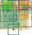
Figure 1: (a) A set of squares $\mathcal{S}$ and a set of points $P$, (b) A set cover (in green) $\mathcal{S}^{\prime}\subseteq\mathcal{S}$ covering $P$, (c) A hitting set (green points) $P^{\prime}\subseteq P$ for $\mathcal{S}$.

Related to set cover is the hitting set problem (see Figure 1 for an illustration) where, given a set of points $P$ and a collection of sets $\mathcal{S}$, we seek to select the minimum number of points $P^{\prime}\subseteq P$ that hit each set $S\in\mathcal{S}$, i.e., such that $P^{\prime}\cap S\neq\emptyset$. Again, in the offline geometric case, there are better approximation ratios known than for the general case, e.g., a PTAS for squares [31], and an $O(\log\log\mathsf{OPT})$-approximation for rectangles [5]. However, in the online and the dynamic cases, only few results are known that improve on the results for the general case. In the online setting, there is an $O(\log n)$-competitive algorithm for $d=1$, i.e., intervals, and an $O(\log n)$-competitive algorithm for unit disks [23]. In the dynamic case, the only known algorithms are for intervals and unit squares (and thus, also for quadrants), yielding approximation ratios of $(1+\varepsilon)$ and $O(1)$, respectively [2].

1.1 Our results

In this paper, we study online algorithms for geometric set cover and hitting set for squares of arbitrary sizes, while previously no improved results were known even for unit squares. Also, we present dynamic algorithms for these problems for hyperrectangles of constant dimension $d$ (also called $d$-boxes or orthotopes) which are far more general geometric objects than those which were previously studied, e.g., intervals [2] or (2-D) squares [20].

Online set cover for squares

In Section 2 we study online set cover for axis-parallel squares of arbitrary sizes and provide an online $O(\log n)$-competitive algorithm. We also match (asymptotically) the lower bound of $\Omega(\log n)$, and hence, our competitive ratio is tight. In our online model (as in [4]), we assume that the sets (squares) are given initially and the elements (points) arrive online.

Our online algorithm is based on a new offline algorithm that is monotone, i.e., it has the property that if we add a new point $p$ to $P$, the algorithm outputs a superset of the squares that it outputs given only $P$ without $p$. The algorithm is based on a quad-tree decomposition. It traverses the tree from the root to the leaves, and for each cell $C$ in which points are still uncovered, it considers each edge $e$ of $C$ and selects the “most useful” squares containing $e$, i.e., the squares with the largest intersection with $C$. We assume (throughout this paper) that all points and all vertices of the squares have integral coordinates in $[0,N)^{2}$ for a given $N$, and we obtain a competitive ratio of $O(\log N)$. If we know that all the inserted points come from an initially given set of $n$ candidate points $P_{0}$ (as in, e.g., Alon et al. [4]), we improve our competitive ratio to $O(\log n)$. For this case, we use the BBD-tree data structure due to Arya et al. [7] which uses a more intricate decomposition into cells than a standard quad-tree, and adapt our algorithm to it in a non-trivial manner. Due to the monotonicity of our offline algorithm, we immediately obtain an $O(\log n)$-competitive online algorithm.

Online hitting set for squares

In Section 3 we present an $O(\log N)$-competitive algorithm for online hitting set for squares of arbitrary sizes, where the points are given initially and the squares arrive online. This matches the best-known $O(\log N)$-competitive algorithm for the much simpler case of intervals [23]. Also, there is a matching lower bound of $\Omega(\log N)$, even for intervals.

In a nutshell, if a new square $S$ is inserted by the adversary, we identify $O(\log N)$ quad-tree cells for which $S$ contains one of its edges. Then, we pick the most useful points in these cells to hit such squares: those are the points closest to the four edges of the cell. We say that this activates the cell. In our analysis, we turn this around: we show that for each point $p\in\mathsf{OPT}$ there are only $O(\log N)$ cells that can possibly get activated if a square $S$ is inserted that is hit by $p$. This yields a competitive ratio of $O(\log N)$.

Dynamic set cover and hitting set for $d$-D hyperrectangles

Then, in Section 4 and 5 we present our dynamic algorithms for set cover and hitting set for hyperrectangles in $d$ dimensions. Note that no dynamic algorithm with polylogarithmic update time and polylogarithmic approximation ratio is known even for set cover for rectangles and it was asked explicitly by Chan et al. [20] whether such an algorithm exists. Thus, we answer this question in the affirmative for the case when only points are inserted and deleted. Note that this is the relevant case when we seek to store our solution explicitly, as discussed above. Even though our considered objects are very general, our algorithms need only polylogarithmic worst-case update time. In contrast, Abboud et al. [1] showed that under Strong Exponential Time Hypothesis any general (dynamic) set cover algorithm with an amortized update time of $O(f^{1-\varepsilon})$ must have an approximation ratio of $\Omega(n^{\alpha})$ for some constant $\alpha>0$, and $f$ can be as large as $\Theta(m)$.

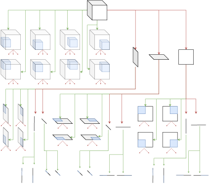
Figure 14: Extended quad-tree with a $2\times 2\times 2$ cube as the root.

We first discuss our algorithm for set cover. We start with reducing the case of hyperrectangles in $d$ dimensions to $2d$-dimensional hypercubes with integral corners in $[0,4m]^{2d}$. Then, a natural approach would be to adapt our algorithm for squares from above to $2d$-dimensional hypercubes. A canonical generalization would be to build a quad-tree, traverse it from the root to the leaves, and to select for each cell $C$ and for each facet $F$ of $C$ the most useful hypercube $S$ containing $F$, i.e., the hypercube $S$ with maximal intersection with $C$. Unfortunately, this is no longer sufficient, not even in three dimensions: it might be that there is a cell $C$ for which it is necessary that we select cubes that contain only an edge of $C$ but not a facet of $C$ (see Figure 2). Here, we introduce a crucial new idea: for each cell $C$ of the (standard) quad-tree and for each dimension $i\in[2d]$, consider the hypercubes which are “edge-covering” $C$ along dimension $i$. Based on these hypercubes a $(2d{-}1)$-dimensional recursive secondary structure is built on all the dimensions except the $i$-th dimension (see Figure 14).

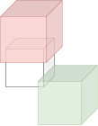
Figure 2: The red cube is the only cube that covers a facet of the (uncolored) cell. The green cube (from $\mathsf{OPT}$) only covers an edge of the cell. Note that there is no corner of a cube from $\mathsf{OPT}$ in the cell. Picking the red cube does not cover the the intersection of the green cube with the cell.

We call the resulting tree the extended quad-tree. Even though it is much larger than the standard quad-tree, we show that each point is contained in only $(\log m)^{O(d)}$ cells. Furthermore, we use it for our second crucial idea to reduce the frequency of the set cover instance: we build an auxiliary instance of general set cover with bounded frequency. It has the same points as the given instance of geometric set cover, but different sets: for each node corresponding to a one-dimensional cell $C$ of the extended quadtree , we consider each of its endpoints $p$ and introduce a set that corresponds to the “most useful” hypercube covering $p$, i.e., the hypercube covering $p$ with maximal intersection with $C$. Since each point is contained in only $(\log m)^{O(d)}$ cells, the resulting frequency is bounded by $(\log m)^{O(d)}$. Also, we show that our auxiliary set cover instance admits a solution with at most $\mathsf{OPT}\cdot(\log m)^{O(d)}$ sets. Then we use a dynamic algorithm from [13] for general set cover to maintain an approximate solution for our auxiliary instance, which yields a dynamic $(\log m)^{O(d)}$-approximation algorithm.

We further adapt our dynamic set cover algorithm mentioned above to hitting set for $d$-dimensional hyperrectangles with an approximation ratio of $(\log n)^{O(d)}$. Finally, we extend our algorithms for set cover and hitting set for $d$-dimensional hyperrectangles even to the weighted case, at the expense of only an extra factor of $(\log W)^{O(1)}$ in the update time and approximation ratio, assuming that all sets/points in the input have weights in $[1,W]$. See the following tables for a summary of our results.

Problem	Objects	Competitive ratio	Lower bound
Set cover	intervals	2 [Thm 7]	2 [Thm 8]
	2-D squares	$O(\log n)$ [Thm 1]	$\Omega(\log n)$ [Thm 1]
Hitting set	intervals	$O(\log N)$ [23]	$\Omega(\log N)$ [23]
	2-D squares	$O(\log N)$ [Thm 3]	$\Omega(\log N)$[23]

Table 1: Online algorithms for geometric set cover and hitting set.

Problem	Objects	Approximation ratio	Update time
Set cover	$2$-D unit squares	$O(1)$ [2]	$(\log n)^{O(1)}$
	$d$-D hyperrectangles	$O(\log^{4d-1}m)\log W$ [Thm 5]	$O(\log^{2d}m)\log^{3}(Wn)$
Hitting set	unit squares	$O(1)$ [2]	$(\log n)^{O(1)}$
	$d$-D hyperrectangles	$O(\log^{4d-1}n)\log W$ [Thm 6]	$O(\log^{2d-1}n)\log^{3}(Wm)$

Table 2: Dynamic algorithms for geometric set cover and hitting set. Update times in [2] are amortized and for the unweighted case. Our results are for worst-case update times.

1.2 Other related work

The general set cover is well-studied in both online and dynamic settings. Several variants and generalizations of online set cover have been considered, e.g., online submodular cover [27], online set cover under random-order arrival [24], online set cover with recourse [25], etc.

For dynamic setting, Gupta et al. [25] initiated the study and provided $O(\log n)$-approximation algorithm with $O(f\log n)$-amortized update time, even in the weighted setting. Similar to our model, in their model sets are given offline and only elements can appear or depart. After this, there has been a series of works [1, 10, 12, 11, 13, 25, 26, 8].

Bhattacharya et al. [13] have given deterministic $(1+\varepsilon)f$-approximation in
$O\left((f^{2}/\varepsilon^{3})+(f/\varepsilon^{2})\log(W)\right)$-amortized update time and $O(f\log^{2}(Wn)/\varepsilon^{3})$-worst-case update time, where $W$ denotes the ratio of the weights of the highest and lowest weight sets. Assadi and Solomon [8] have given a randomized $f$-approximation algorithm with $O(f^{2})$-amortized update time.

Agarwal et al. [2] studied another dynamic setting for geometric set cover, where both points and sets can arrive or depart, and presented $(1+\varepsilon)$- and $O(1)$-approximation with sublinear update time for intervals and unit squares, respectively. Chan and He [19] extended it to set cover with arbitrary squares. Recently, Chan et al. [20] gave $(1+\varepsilon)$-approximation for the special case of intervals in $O(\log^{3}n/\varepsilon^{3})$-amortized update time. They also gave $O(1)$-approximation for dynamic set cover for unit squares, arbitrary squares, and weighted intervals in amortized update time of $2^{O(\sqrt{\log n})},n^{1/2+\varepsilon}$, and $2^{O(\sqrt{\log n\log\log n})}$, respectively.

Dynamic algorithms are also well-studied for other geometric problems such as maximum independent set of intervals and hyperrectangles [29, 14, 17], and geometric measure [22].

2 Set cover for squares

In this section we present our online and dynamic algorithms for set cover for squares. We are given a set of $m$ squares $\mathcal{S}$ such that each square $S\in\mathcal{S}$ has integral corners in $[0,N)^{2}$. W.l.o.g. assume that $N$ is a power of 2. We first describe an offline $O(\log N)$-approximate algorithm. Then we construct an online algorithm and a dynamic algorithm based on it, such that both of them have approximation ratios of $O(\log N)$ as well. For our offline algorithm, we assume that in addition to $\mathcal{S}$ and $N$, we are given a set of points $P$ that we need to cover, such that $P\subseteq[0,N)^{2}$ and each point $p\in P$ has integral coordinates.

Quad-tree

We start with the definition of a quad-tree $T=(V,E)$, similarly as in, e.g., [6, 9]. In $T$ each node $v\in V$ corresponds to a square cell $C_{v}\subseteq[0,N)^{2}$ whose vertices have integral coordinates. The root $r\in V$ of $T$ corresponds to the cell $C_{r}:=[0,N)^{2}$. Recursively, consider a node $v\in V$, corresponding to a cell $C_{v}$ and assume that $C_{v}=[x_{1}^{(1)},x_{2}^{(1)})\times[x_{1}^{(2)},x_{2}^{(2)})$. If $C_{v}$ is a unit square, i.e., $|x_{2}^{(1)}-x_{1}^{(1)}|=|x_{2}^{(2)}-x_{1}^{(2)}|=1$, then we define that $v$ is a leaf. Otherwise, we define that $v$ has four children $v_{1},v_{2},v_{3},v_{4}$ that correspond to the four cells that we obtain if we partition $C_{v}$ into four equal sized smaller cells, i.e., define $x_{\text{$\mathrm{mid}$}}^{(1)}:=(x_{2}^{(1)}-x_{1}^{(1)})/2$ and $x_{\text{$\mathrm{mid}$}}^{(2)}:=(x_{2}^{(2)}-x_{1}^{(2)})/2$ and $C_{v_{1}}=[x_{1}^{(1)},x_{\text{$\mathrm{mid}$}}^{(1)})\times[x_{1}^{(2)},x_{\text{$\mathrm{mid}$}}^{(2)})$, $C_{v_{2}}=[x_{1}^{(1)},x_{\text{$\mathrm{mid}$}}^{(1)})\times[x_{\text{$\mathrm{mid}$}}^{(2)},x_{2}^{(2)})$, $C_{v_{3}}=[x_{\text{$\mathrm{mid}$}}^{(1)},x_{2}^{(1)})\times[x_{1}^{(2)},x_{\text{$\mathrm{mid}$}}^{(2)})$, and $C_{v_{4}}=[x_{\text{$\mathrm{mid}$}}^{(1)},x_{2}^{(1)})\times[x_{\text{$\mathrm{mid}$}}^{(2)},x_{2}^{(2)})$. Note that the depth of this tree is $\log N$, where depth of a node in the tree is its distance from the root of $T$, and depth of $T$ is the maximum depth of any node in $T$. By the construction, each leaf node contains at most one point and it will lie on the bottom-left corner of the corresponding cell.

Offline algorithm

In the offline algorithm $\mathcal{A}_{\text{off}}$, we traverse $T$ in a breadth-first-order, i.e., we order the nodes in $V$ by their distances to the root $r$ and consider them in this order (breaking ties arbitrarily but in a fixed manner). Suppose that in one iteration we consider a node $v\in V$, corresponding to a cell $C_{v}$. We check whether the squares selected in the ancestors of $v$ cover all points in $P\cap C_{v}$. If this is the case, we do not select any squares from $\mathcal{S}$ in this iteration (corresponding to $v$). Observe that hence we also do not select any squares in the iterations corresponding to the descendants of $v$ in $T$ (so we might as well skip the whole subtree rooted at $v$).

Suppose now that the squares selected in the ancestors of $v$ do not cover all points in $P\cap C_{v}$. We call such a node to be explored by our algorithm. Let $e$ be an edge of $C_{v}$. We say that a square containing $e$ is edge-covering for $e$. We select a square from $\mathcal{S}$ that is edge-covering for $e$ and that has the largest intersection with $C_{v}$ among all such squares in $\mathcal{S}$ (we call such a square maximum area-covering for $C_{v}$ for edge $e$). We break ties in an arbitrary but fixed way, e.g., by selecting the square with smallest index according to an arbitrary ordering of $\mathcal{S}$. If there is no square in $\mathcal{S}$ that is edge-covering for $e$ then we do not select a square corresponding to $e$. We do this for each of the four edges of $C_{v}$. See Figure 3. If we reach a leaf node, and if there is an uncovered point (note that it must be on the bottom-left corner of the cell), then we select any arbitrary square that covers the point (the existence of such a square is guaranteed as some square in $\mathsf{OPT}$ covers it). See Figure 4.

Figure 3: Left figure shows a quad-tree cell in purple. The maximum area-covering square (solid black) is picked, while the other edge-covering squares (dashed) are not. Right figure shows the quad-tree cells (level-wise color-coded) containing an uncovered point. In increasing order of depth of these cells, at most $4$ maximum-area covering squares (solid black) are picked together per cell, till the point gets covered.

Figure 4: Point $p$ lies in a leaf cell $C$ (which may not even have any edge-covering squares). In this case, we pick an arbitrary square $S$ to cover the point (since one such square always exists).

Lemma 1.

$\mathcal{A}_{\text{off}}$ outputs a feasible set cover for the points in $P$.

Proof.

Assume for contradiction that no square in ALG covered some point $p\in P$. Since $\mathsf{OPT}$ is a feasible set cover, there is a square $S\in\mathsf{OPT}$ which covered $p$. There are two cases to consider here: either $p$ is exactly at one of the corners of $S$, or not. In the latter case, note that $S$ is edge-covering for at least one quad-tree cell containing $p$. Let $C_{v}$ be such a cell (which contains $p$ and its edge $e$ is contained in $S$) with minimum depth. Now the algorithm will traverse $T$ till we reach the node $v$ (corresponding to cell $C_{v}$) containing $p$. As the squares selected by the algorithm for the ancestors of $v$ do not cover $p$, we will select the maximum area-covering square $S^{\prime}$ (for $e$) in ALG. As $(S\cap C_{v})\subseteq(S^{\prime}\cap C_{v})$, $S^{\prime}$ will cover $p$. This is a contradiction. Now in the first case, i.e., where $p$ is at one of the corners of $S\in\mathsf{OPT}$, either there is a leaf $v\in T$ which contains it and $S$ is edge-covering for $C_{v}$, or for such a leaf $v$, $S$ is corner-covering. In both the cases, $\mathcal{A}_{\text{off}}$ will pick a square for $v$ or one of its ancestors such that this square covers $p$. ∎

Approximation ratio

Let $\mathsf{ALG}\subseteq\mathcal{S}$ denote the selected set of squares and let $\mathsf{OPT}$ denote the optimal solution. To prove the $O(\log N)$-approximation guarantee, the main idea is the following: consider a node $v\in V$ and suppose that we selected at least one square in the iteration corresponding to $v$. If $C_{v}$ contains a corner of a square $S\in\mathsf{OPT}$, then we charge the (at most four) squares selected for $v$ to $S$. Otherwise, we argue that the squares selected for $v$ cover at least as much of $C_{v}$ as the squares in $\mathsf{OPT}$, and that they cover all the remaining uncovered points in $P\cap C_{v}$. In particular, we do not select any further squares in the descendants of $v$. The squares selected for $v$ are charged to the parent of $v$ (which contains a corner of a square $S\in\mathsf{OPT}$). Since each corner of each square $S\in\mathsf{OPT}$ is contained in $O(\log N)$ cells, we show that each square $S\in\mathsf{OPT}$ receives a total charge of $O(\log N)$. Thus, we obtain the following lemma.

Lemma 2.

We have that $|\mathsf{ALG}|=O(\log N)\cdot|\mathsf{OPT}|$.

Proof.

We will charge each square picked in $\mathsf{ALG}$ to some square in $\mathsf{OPT}$. A cell $C_{v}$ with its corresponding node $v$, can either contain (at least) a corner of some square in $\mathsf{OPT}$, or be edge-covered by (at least) a square in $\mathsf{OPT}$, or not intersect any square from $\mathsf{OPT}$ at all.

• $C_{v}$ contains a corner of $S\in\mathsf{OPT}$: In this case, $\mathcal{A}_{\text{off}}$ picks at most four squares for the cell, and we charge these squares to a corner of $S$ in the cell. If there are multiple squares from $\mathsf{OPT}$ with a corner in the cell, pick one arbitrarily. This claim is true even when $C_{v}$ corresponds to a leaf node.

• Some square $S\in\mathsf{OPT}$ is edge-covering for $C_{v}$ (and $C_{v}$ has no corner of a square in $\mathsf{OPT}$): If $\mathcal{A}_{\text{off}}$ picks no edge-covering squares for such a cell, then we are fine. Otherwise, if $\mathcal{A}_{\text{off}}$ picks squares for such a cell, we claim that it covers all points in the cell. This is due to the fact that any point in this cell is covered by a square in $\mathsf{OPT}$ that is edge-covering for $C_{v}$, due to the absence of corners of squares of $\mathsf{OPT}$. So when $\mathcal{A}_{\text{off}}$ picks edge-covering squares with the largest intersection with the cell, the intersection of any square $S^{\prime}\in\mathsf{OPT}$ with $C_{v}$ will also get covered). So, no child node of $v$ will be further explored by the algorithm. This also means that the parent $v^{\prime}$ of $v$ in the tree will contain a corner of $S$ (because $C_{v^{\prime}}$ intersects $S$, but cannot be edge-covered by it). We charge any squares picked by $\mathcal{A}_{\text{off}}$ at $C_{v}$ (at most four times) to this particular corner in the parent node. If there are multiple such corners, pick one arbitrarily.

• No squares from $\mathsf{OPT}$ intersect $C_{v}$: In this case, $C_{v}$ does not contain any points in $P$. Thus, $\mathcal{A}_{\text{off}}$ will not pick any squares for such a cell.

Figure 5: Charging picked (red) edge-covering squares to the corner of a (cyan) square in $\mathsf{OPT}$. In the image on the left, the (yellow) cell contains a corner of the square from $\mathsf{OPT}$, and in the image on the right, the parent of the cell contains such a corner.

Now we note that a corner of any square in $\mathsf{OPT}$, will lie in at most $\log N$ cells of the quad-tree. For each of these cells, a corner is charged at most four times for the squares picked at the cell, and at most four times for each of its four child nodes. This amounts to a total charge of at most 20 per corner per cell. So each square in $\mathsf{OPT}$ is charged at most $20\text{ (per corner, per cell)}\times 4\text{ (corners)}\times\log N\text{ (cells)}=80\log N$ times. Therefore, there are at most $80\log N\cdot|\mathsf{OPT}|$ squares in $\mathsf{ALG}$. ∎

2.1 Online set cover for squares

2.1.1 $O(\log N)$-approximate online algorithm

We want to turn our offline algorithm $\mathcal{A}_{\text{off}}$ into an online algorithm $\mathcal{A}_{\text{on}}$, assuming that in each round a new point is introduced by the adversary. The key insight for this is that the algorithm above is monotone, i.e., if we add a point to $P$, then it outputs a superset of the squares from $\mathcal{S}$ that it had output before (when running it on $P$ only). For a given set of points $P$, let $\mathsf{ALG}(P)\subseteq\mathcal{S}$ denote the set of squares that our (offline) algorithm outputs.

Lemma 3.

Consider a set of points $P$ and a point $p$. Then $\mathsf{ALG}(P)\subseteq\mathsf{ALG}(P\cup\{p\})$.

Proof.

Assume towards contradiction that there exists some square $S$ in $\mathsf{ALG}(P)$ which did not belong to $\mathsf{ALG}(P\cup\{p\})$. According to the description of $\mathcal{A}_{\text{off}}$, we can infer that $S$ was picked by the algorithm in some iteration because it was maximum area-covering for some cell $C_{v}$ (corresponding to node $v$ in $T$) that contained a point $p^{\prime}\in P$ introduced by the adversary. Also, $\mathcal{A}_{\text{off}}$ in its run must have explored all the ancestors of $v$ in $T$. Note that any such point $p^{\prime}$ could be covered in a run of the algorithm only when it traverses cells that contain $p^{\prime}$. This is due to the fact that once we pick some squares associated with a cell in the quad-tree, we only account for the area inside this cell that the squares cover. In light of this fact, if $\mathcal{A}_{\text{off}}$ did not explore $C_{v}$ in this time step, then it also would not have explored the children of $v$ in $T$. Hence, the point $p^{\prime}$ would not have been covered which is a contradiction. ∎

Hence, it is easy now to derive an online algorithm for set cover for squares. Initially, $P=\emptyset$. If a point $p$ is introduced by the adversary, then we compute $\mathsf{ALG}(P)$ (where $P$ denotes the set of previous points, i.e., without $p$) and $\mathsf{ALG}(P\cup\{p\})$ and we add the squares in $\mathsf{ALG}(P\cup\{p\})\setminus\mathsf{ALG}(P)$ to our solution. Therefore, due to Lemma 2 and Lemma 3 we obtain an $O(\log N)$-competitive online algorithm.

2.1.2 $O(\log n)$-approximate online set cover for squares

We assume now that we are given a set $\tilde{P}\subseteq\mathbb{R}^{2}$ with $|\tilde{P}|=n$ such that in each round a point from $\tilde{P}$ is inserted to $P$, i.e., $P\subseteq\tilde{P}$ after each round. We want to get a competitive ratio of $O(\log n)$ in this case. If $N=n^{O(1)}$ then this is immediate. Otherwise, we extend our algorithm such that it uses the balanced box-decomposition tree (or BBD-tree) data structure due to Arya et al. [7], instead of the quad-tree. Before the first round, $P=\emptyset$ and we initialize the BBD-tree which yields a tree $\tilde{T}=(\tilde{V},\tilde{E})$ with the following properties:

• each node $v\in\tilde{V}$ corresponds to a cell $\tilde{C}_{v}\subseteq[0,N)^{2}$ which is described by an outer box $b_{O}\subseteq[0,N)^{2}$ and an inner box $b_{I}\subseteq b_{O}$; both of them are axis-parallel rectangles and $\tilde{C}_{v}=b_{O}\setminus b_{I}$ (Note that $b_{I}$ could be the empty set).

• the aspect ratio of $b_{O}$, i.e., the ratio between the length of the longest edge to the length of the shortest edge of $b_{O}$, is bounded by 3.

• if $b_{I}\neq\emptyset$, then $b_{I}$ is sticky which intuitively means that in each dimension, the distance of $b_{I}$ to the boundary of $b_{O}$ is either 0 or at least the width of $b_{I}$. Formally, assume that $b_{O}=[x_{O}^{(1)},x_{O}^{(2)}]\times[y_{O}^{(1)},y_{O}^{(2)}]$ and $b_{I}=[x_{I}^{(1)},x_{I}^{(2)}]\times[y_{I}^{(1)},y_{I}^{(2)}]$. Then $x_{O}^{(1)}=x_{I}^{(1)}$ or $x_{I}^{(1)}-x_{O}^{(1)}\geq x_{I}^{(2)}-x_{I}^{(1)}$. Also $x_{O}^{(2)}=x_{I}^{(2)}$ or $x_{O}^{(2)}-x_{I}^{(2)}\geq x_{I}^{(2)}-x_{I}^{(1)}$. Analogous conditions also hold for the $y$-coordinates.

• each node $v\in\tilde{V}$ is a leaf or it has two children $v_{1},v_{2}\in\tilde{V}$; in the latter case $\tilde{C}_{v}=\tilde{C}_{v_{1}}\dot{\cup}\tilde{C}_{v_{2}}$.

• the depth of $\tilde{T}$ is $O(\log n)$ and each point $q\in[0,N)^{2}$ is contained in $O(\log n)$ cells.

• each leaf node $v\in\tilde{V}$ contains at most one point in $\tilde{P}$.

In the construction of the BBD-tree, we make the cells at the same depth disjoint so that a point $p$ may be contained in exactly one cell at a certain depth. Hence, for a cell $\tilde{C}_{v}=b_{O}\setminus b_{I}$ we assume both $b_{O}$ and $b_{I}$ to be closed set, i.e., the boundary of the outer box $b_{O}$ is part of the cell and the boundary of the inner box $b_{I}$ is not part of the cell. We now describe an adjustment of our offline algorithm from Section 2, working with $\tilde{T}$ instead of $T$. Similarly, as before, we traverse $\tilde{T}$ in a breadth-first-order. Suppose that in one iteration we consider a node $v\in\tilde{V}$ corresponding to a cell $\tilde{C}_{v}$. We check whether the squares selected in the ancestors of $v$ cover all points in $P\cap\tilde{C}_{v}$. If this is the case, we do not select any squares from $\mathcal{S}$ in this iteration corresponding to $v$.

Suppose now that the squares selected in the ancestors of $v$ do not cover all points in $P\cap\tilde{C}_{v}$. Similar to Section 2, we want to select $O(1)$ squares for $\tilde{C}_{v}$ such that if $\tilde{C}_{v}$ contains no corner of a square $S\in\mathsf{OPT}$, then the squares we selected for $\tilde{C}_{v}$ should cover all points in $P\cap\tilde{C}_{v}$. Similarly as before, for each edge $e$ of $b_{O}$ we select a square from $\mathcal{S}$ that contains $e$ and that has the largest intersection with $b_{O}$ among all such squares in $\mathcal{S}$. We break ties in an arbitrary but fixed way. However, as $\tilde{C}_{v}$ may not be a square and can have holes (due to $b_{I}$), apart from the edge-covering squares, we need to consider two additional types of squares in $\mathsf{OPT}$ with nonempty overlap with $\tilde{C}_{v}$: (a) crossing $\tilde{C}_{v}$, i.e., squares that intersect two parallel edges of $b_{O}$; (b) has one or two corners inside $b_{I}$.

The following greedy subroutine $\mathcal{G}$ will be useful in our algorithm to handle such problematic cases. Let $R$ be a box of width $w$ and height $h$ such that $w/h\leq B$, for some constant $B\in\mathbb{N}$; and $P_{R}$ be a set of points inside $R$ that can be covered by a collection of vertically-crossing (i.e., they intersect both horizontal edges of $R$) squares $\mathcal{S}^{\prime}$. Then, the set of squares picked according to $\mathcal{G}$ covers $P_{R}$ in the following way:

• While there is an uncovered point $p^{\prime}\in P_{R}$:

  • Consider the leftmost such uncovered point $p\in P_{R}$.

  • Select the vertically-crossing square intersecting $p$ (by assumption, such a square exists) with the rightmost edge.

(The above subroutine is for finding vertically-crossing squares. For finding horizontally-crossing squares, we can appropriately rotate the input $90^{\circ}$ anti-clockwise, and apply the same subroutine.) Then, we have the following claim about the aforementioned subroutine.

Claim 1.

Let $R$ be a box of width $w$ and height $h$ such that $w/h\leq B$, for some constant $B\in\mathbb{N}$; and $P_{R}$ be a set of points inside $R$ that can be covered by a collection of vertically-crossing (i.e., they intersect both horizontal edges of $R$) squares $\mathcal{S}^{\prime}$. Then we can find at most $B+1$ squares from $\mathcal{S}^{\prime}$ that can cover all points inside $R$.

We have an analogous claim for horizontally-crossing squares when $h/w\leq B$.

Proof.

Consider each iteration of the greedy subroutine $\mathcal{G}$. We call pivot to be the leftmost point $p\in P_{R}$ that is not already covered by a square selected by $\mathcal{G}$ so far. Then all selected vertically-crossing squares for $R$ will contain exactly one point that was identified as a pivot point at some point during the execution of the algorithm. As the aspect ratio is bounded by $B$ and the squares are vertically-crossing (i.e., their vertical length is more than the vertical length of $R$), there can be at most $B+1$ pivot points. Hence, we select at most $B+1$ crossing squares due to $R$. This produces a feasible set cover. ∎

Now we describe our algorithm. First, we take care of the squares that can cross $b_{O}$. So, we apply the greedy subroutine $\mathcal{G}$ on $b_{O}$. As $b_{O}$ has bounded aspect ratio of 3, from Claim 1, we obtain at most $(3+1)+(1+1)=6$ squares that can cross $C_{v}$ vertically or horizontally. If $b_{I}=\emptyset$, we do not select any more squares. Otherwise, we need to take care of the squares that can have one or two corners inside $b_{I}$. Let $\ell_{1},\ell_{2},\ell_{3},\ell_{4}$ denote the four lines that contain the four edges of $b_{I}$. Observe that $\ell_{1},\ell_{2},\ell_{3},\ell_{4}$ partition $b_{O}$ into up to nine rectangular regions, one being identical to $b_{I}$. For each such rectangular region $R$, if it is sharing a horizontal edge with $b_{I}$, we again use $\mathcal{G}$ to select vertically-crossing squares. Otherwise, if $R$ is sharing a vertical edge with $b_{I}$, we use the subroutine $\mathcal{G}$ appropriately to select horizontally-crossing squares. This takes care of squares having two corners inside $b_{I}$. Otherwise, if the rectangular region $R$ does not share an edge with $b_{I}$, then we check if there is a square $S\in\mathcal{S}$ with a corner within $b_{I}$ that completely contains $R$. We add $S$ to our solution too. This finally takes care of the case when a square has a single corner inside $b_{I}$.

Finally, to complete our algorithm, before its execution, we do the following: for every leaf $v$ for which $C_{v}$ contains at most one point $p\in\tilde{P}$, we associate a fixed square which covers $p$. Then, if our algorithm reaches a leaf $v$ while traversing that has an uncovered point $p$, we pick the associated square with this leaf that covers it. This condition in our algorithm guarantees feasibility.

Figure 6: Outer box $b_{O}$ being partitioned into at most 9 rectangles due to inner box $b_{I}$.

Figure 7: Possible intersections of a (cyan) square from $\mathsf{OPT}$ with a cell, such that no corner of the square is in the cell. The left image shows edge-covering, and crossing squares. The right image shows squares with one of two corners inside $b_{I}$.

Lemma 4.

Let $\tilde{C}_{v}$ be a cell such that the squares selected in the ancestors of $v$ do not cover all points in $P\cap\tilde{C}_{v}$. Then

1. we select at most $O(1)$ squares for $\tilde{C}_{v}$ and

2. if $\tilde{C}_{v}$ contains no corner of a square $S\in\mathsf{OPT}$, then the squares we selected for $\tilde{C}_{v}$ cover all points in $P\cap\tilde{C}_{v}$.

Proof.

First, we prove part (a). If $\tilde{C}_{v}$ corresponds to a leaf node, we select at most one square. Otherwise, We select at most 4 edge-covering squares for $\tilde{C}_{v}$. From Claim 1, we select $O(1)$ number squares for $\tilde{C}_{v}$ that are horizontally or vertically-crossing $b_{O}$. We select no more squares if $b_{I}=\emptyset$.

So consider the other case: $b_{I}\neq\emptyset$. Let $R$ be one of the (at most) four rectangular regions obtained from partitioning of $b_{O}$ (by $\ell_{1},\ell_{2},\ell_{3},\ell_{4}$) that share an edge with $b_{I}$. Let $w,h$ be width and height of $R$, respectively. W.l.o.g. assume $R$ shares a horizontal edge with $b_{I}$. As $b_{I}$ is sticky, and $b_{I}$ and $b_{O}$ have a bounded aspect ratio of 3, it can be seen that $R$ also has a $w/h\leq 3$ (similarly, if $R$ shared a vertical edge with $b_{I}$, then $h/w\leq 3$). Again using Claim 1, we select $O(1)$ vertically-crossing squares for $R$. We do a similar operation for other such regions. Now consider the remaining (at most four) regions obtained from partitioning of $b_{O}$ (by $\ell_{1},\ell_{2},\ell_{3},\ell_{4}$) that do not share an edge with $b_{I}$. We select at most one square for each of them. Thus, in total, we select at most $O(1)$ squares for $\tilde{C}_{v}$.

Now we prove part (b). If $\tilde{C}_{v}$ contains no corner of a square $S\in\mathsf{OPT}$, then all the squares in $\mathsf{OPT}$ that intersect $\tilde{C}_{v}$ are either edge-covering $b_{O}$, or crossing $\tilde{C}_{v}$, or contain one or two corners inside $b_{I}$. However, as we have picked maximal edge-covering squares for $b_{O}$, they contain all points in $\tilde{C}_{v}$ that are covered by the edge-covering squares from $\mathsf{OPT}$.

Similarly, by our selected squares (that vertically or horizontally crosses $b_{O}$) in the greedy subroutine $\mathcal{G}$, we have covered all points that can be covered by such crossing squares in $\mathsf{OPT}$ that crosses $b_{O}$.

For squares that have (at least) a corner inside $b_{I}$, note that they have to cross one of the rectangular regions that came from partitioning of $b_{O}$ and shares an edge with $b_{I}$. In fact, for such a square $S$ with a corner inside $b_{I}$, there is a rectangular region $R$ (say, with width $w$ and height $h$) among these four rectangular regions such that either $S$ is vertically-crossing for $R$ and $R$ shared a horizontal edge with $b_{I}$ (then $w/h\leq 3$) or $S$ is horizontally-crossing for $R$ and $R$ shared a vertical edge with $b_{I}$ (then $h/w\leq 3$). But then using Claim 1, we cover all points covered by such squares. Additionally, a square that has exactly one corner inside $b_{I}$ may completely contain another rectangular region from partitioning of $b_{O}$ (that do not share an edge with $b_{I}$). For them, again we have covered them by selecting one square, if it exists. ∎

Thus, we can establish a similar charging scheme as in Section 2. To pay for our solution, we charge each corner $q$ of a square $S\in\mathsf{OPT}$ at most $O(\log n)$ times. Hence, our approximation ratio is $O(\log n)$. Similarly as in Section 2, we can modify the above offline algorithm to an online algorithm with an approximation ratio of $O(\log n)$ each.

Theorem 1.

There is a deterministic $O(\log n)$-competitive online algorithm for set cover for axis-parallel squares of arbitrary sizes.

2.2 Lower bounds

It is a natural question whether algorithms having a competitive factor better than $O(\log n)$ are possible for online set cover for squares. We answer this question in the negative, even for the case of unit squares and even for randomized algorithms. We also remark here that there exists a tight $2$-competitive online algorithm for set cover for intervals (see Section A).

2.2.1 Unit squares and quadrants

Given a set cover instance $(P,\mathcal{F})$, for each $F\in\mathcal{F}$ define a variable $x_{F}$ which takes values $\in[0,1]$. For a point $p\in P$, let $\mathcal{F}_{p}\subseteq\mathcal{F}$ be the sets that cover it. In the fractional set cover problem, the aim is to assign values to the variables $x_{F}$ such that for all points $p\in P$, $\sum_{F\in\mathcal{F}_{p}}x_{F}\geq 1$.

Figure 8: $\Omega(\log m)$ hard instances for quadrants and unit squares

Lemma 5.

There is an instance of the online fractional covering problem on $m$ quadrants (quadrant is a rectangle with one of its corners as the origin) such that any online deterministic algorithm is $\Omega(\log m)$-competitive on this instance.

Proof.

Consider the set of $m$ quadrants (See Figure 8) with their top-right corners as follows: $Q_{1}=(1,m),Q_{2}=(2,m-1),\dots,Q_{k}=(k,m-k+1),\dots,Q_{m}=(m,1)$ (and let the corresponding variables for the set cover instance be $x_{1},x_{2},\dots,x_{m}$, respectively). Now consider a point $p_{i,j}=(i-0.5,m-j+0.5)$. We claim that this point intersects exactly the $i^{th}$ to $j^{th}$ indexed quadrants. Since $p(x)>i-1$, $p_{i,j}$ does not intersect any of the first $(i-1)$ quadrants. Additionally since $p(y)=m-j+0.5<m-i-1$ it does intersect quadrant $i$ and this holds true up to quadrant $j$ (Since, $p(y)=m-j+0.5<m-i-1$). Also $p_{i,j}$ does not intersect any of the last $m-j+1$ quadrants because $p(y)>m-j$.

Now consider an adversary that introduces points as follows: $P_{1}=p_{1,m}$. If the algorithm assigns values to the variables such that $\sum_{i=1}^{m/2}x_{i}\geq\sum_{i=m/2+1}^{i=m}x_{i}$, then the point $P_{2}=p_{m/2+1,m}$ is given, otherwise the point $P_{2}=p_{1,m/2}$ is given. The adversary repeats this process of halving the set of quadrants intersected, and puts the next point in the range with the lower sum, till only one quadrant, say quadrant $j$ is left.

The optimal solution would have been to assign only $x_{j}$ to 1 and the remaining variables to zero. But any online algorithm can only halve the set of the potential optimal solution in each step, while assigning at least $1/2$ “cost” to the non-optimal quadrants. Hence, the cost of any online algorithm is $\Omega(\log m)$. ∎

Corollary 1.

There is an instance of the online fractional covering problem on $m$ unit squares such that any deterministic online algorithm is $\Omega(\log m)$-competitive on this instance.

Proof.

We can appropriately extend the quadrants from Lemma 5 in the bottom-left direction to obtain a similar instance on squares with side-length of $m$. More precisely, let the bottom left corner of the square $i$ corresponding to quadrant $i$ be $(i-m,1-i)$. The points introduced by the adversary are the same as in the quadrants instance.

Now scale down this instance on squares appropriately, by a factor of $m$, to get the required unit square instance. ∎

Using standard techniques, as in [15], we can extend the lower bound for deterministic algorithms for the fractional variant to the lower bound for randomized algorithms for the integral variant.

Corollary 2.

There is an instance of the online (integral) set cover problem on $m$ unit squares such that any randomized online algorithm is $\Omega(\log m)$-competitive on this instance.

Since in our lower bound construction, $n=\Theta(m^{2})$, $\log n=\Theta(\log m)$ and hence, we have the theorem as stated below.

Theorem 2.

Any deterministic or randomized online algorithm for set cover for unit squares has a competitive ratio of $\Omega(\log n)$, even if all squares contain the origin and all points are contained in the same quadrant.

3 Online hitting set for squares

We present our online algorithm for hitting set for squares. We assume that we are given a fixed set of points $P\subseteq[0,N)^{2}$ with integral coordinates. We maintain a set $P^{\prime}$ of selected points such that initially $P^{\prime}:=\emptyset$. In each round, we are given a square $S\subseteq[0,N)^{2}$ whose corners have integral coordinates.

We assume w.l.o.g. that $N$ is a power of 2. Let $Q$ be all points with integral coordinates in $[0,N)^{2}$, i.e., $P\subseteq Q$. For each point $q\in Q$ we say that $q=(q_{x},q_{y})$ is of level $\ell$ if both $q_{x}$ and $q_{y}$ are integral multiples of $N/2^{\ell}$. We build the same quad-tree as in Section 2. We say that a cell $C_{v}$ is of level $\ell$ if its height and width equal $N/2^{\ell}$.

We present our algorithm now. Suppose that in some round a new square $S$ is given. If $S\cap P^{\prime}\neq\emptyset$ then we do not add any point to $P^{\prime}$. Suppose now that $S\cap P^{\prime}=\emptyset$. Let $q$ be a point of smallest level among all points in $Q\cap S$ (if there are many such points, then we select an arbitrary point in $Q\cap S$ of smallest level). Intuitively, we interpret $q$ as if it were the origin and partition the plane into four quadrants. We define $O_{TR}:=\{(p_{x},p_{y})\mid p_{x}\geq q_{x}\,,\,p_{y}\geq q_{y}\}$, and $S_{TR}:=O_{TR}\cap S$, and define similarly $O_{TL},O_{BR},O_{BL}$, and $S_{TL},S_{BR},S_{BL}$. Consider $O_{TR}$ and $S_{TR}$. For each level $\ell=0,1,\dots,\log N$, we do the following. Consider each cell $C$ of level $\ell$ in some fixed order such that $C\subseteq O_{TR}$ and $S_{TR}$ is edge-covering for some edge $e$ of $C$. Then, for each edge identify the point $p_{b}$ ($p_{t},p_{l},p_{r}$, resp.) in $P\cap C$ that is closest to its bottom (top, left, and right, resp.) edge. We add these (at most 4) points to our solution if at least one of $p_{b},p_{t},p_{l},p_{r}$ is contained in $S_{TR}$ (see Figure 9). If we add at least one such point $p$ of the cell $C$ to $P^{\prime}$ in this way, we say that $C$ gets activated. Note that we add possibly all of the points $p_{b},p_{t},p_{l},p_{r}$ to $P^{\prime}$ even though only one may be contained in $S_{TR}$. This is to ensure that $C$ gets activated at most once during a run of the online algorithm. This will be proved in Claim 2, which will ultimately help us prove that our algorithm is $O(\log N)$-competitive. If for the current level $\ell$ we activate at least one cell $C$ of level $\ell$, then we stop the loop and do not consider the other levels $\ell+1,\dots,\log N$. Otherwise, we continue with level $\ell+1$. We do a symmetric operation for the pairs ($O_{TL},S_{TL}$), ($O_{BR},S_{BR}$), and ($O_{BL},S_{BL}$). We now prove the correctness of the algorithm and that its competitive ratio is $O(\log N)$.

Figure 9: In cell $C$ lying in $O_{\text{TR}}$ the red points are chosen by the algorithm.

Lemma 6.

After each round, the set $P^{\prime}$ is a hitting set for the squares that have been added so far.

Proof.

We will prove that in case $S\cap P^{\prime}=\emptyset$ when a square $S$ is inserted, at least one cell $C$ gets activated. Note that there exists a point $p$ in an optimum hitting set such that $p\in S$. Assume w.l.o.g. that $p$ belongs to $S_{TR}$. Then, consider the set of cells $\mathcal{C}_{p}^{\prime}$ that contain the point $p$. Since $S$ has side-length at least $1$ (it has integral coordinates for the corners) there exists a cell $C^{\prime}\in\mathcal{C}_{p}^{\prime}$ such that $S_{TR}$ covers an edge $e$ of $C^{\prime}$. Hence, there will exist one level $\ell$ in $\{0,1,...,\log N\}$ such that a cell $C^{\prime\prime}\subseteq O_{TR}$ of level $\ell$ exists for which $S$ covered its edge (say, the bottom edge $e^{\prime}$) and $p\in C^{\prime\prime}\cap S$. Then, our algorithm picked $p_{b}$ (point closest to the bottom edge) for $C^{\prime\prime}$, such that $p_{b}\in C^{\prime\prime}\cap S$. ∎

Now we show that in each round $O(1)$ points are added to $P^{\prime}$.

Lemma 7.

In each round we add $O(1)$ points to $P^{\prime}$.

Proof.

We show that given a square $S$ such that $S\cap P^{\prime}=\emptyset$ ($P^{\prime}$ is the hitting set maintained by our algorithm), our algorithm activates at most $4$ cells. For this, we just observe that in each of the four quadrants $O_{TR},O_{BR},O_{TL},O_{BL}$, we activate at most $1$ cell. For each of these cells, we pick at most $4$ points and hence, we add at most $16$ points in any round. ∎

Denote by $\mathsf{OPT}$ the optimal solution after the last round of inserting a square.

Lemma 8.

Let $p\in\mathsf{OPT}$. Then there are $O(\log N)$ rounds in which a square $S$ with $p\in S$ was inserted, such that at the beginning of the round $P^{\prime}\cap S=\emptyset$.

Proof.

First, define horizontal distance between two cells of level $\ell$ to be the distance between the $x$-coordinates of their left edges. Analogously, define the vertical distance. Now, we define a set of cells $\mathcal{C}_{p}$ corresponding to the point $p$, initialized to $\emptyset$. We will show later that in a certain round if a square $S$ introduced by the adversary contains $p$, and our algorithm activates at least one cell, then one cell in $\mathcal{C}_{p}$ is also activated. For each level $\ell\in\{0,1,\dots,\log N\}$, include in the set $\mathcal{C}_{p}$: the cell $C$ of level $\ell$ containing $p$ and the other cells of level $\ell$ if they exist which have the same parent as $C$. We call these cells to be primary cells. Further, for level $\ell\in\{0,1,\dots,\log N\}$ consider the cell $C$ of level $\ell$ which contains $p$. Then, consider all the cells of level $\ell$ which are at a distance of $N/2^{\ell}$ horizontally but at a distance of $0$ vertically; also, consider cells which are at a distance of $N/2^{\ell}$ vertically but at a distance of $0$ horizontally from $C$. There can be at most $4$ such cells. For each such cell, include all its children in $\mathcal{C}_{p}$ (which are $4$ in number). We call these cells to be secondary cells. Hence, per level we select at most $4+4\times 4=20$ cells. Therefore, $|\mathcal{C}_{p}|=O(\log N)$.

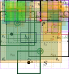
Figure 10: Cell $C$ contains point $p$. The primary cells are highlighted in green, while the secondary cells are highlighted in pink.

We first observe that once a cell $\hat{C}$ gets activated, it does not get activated again.

Claim 2.

A cell $\hat{C}\in T$ does not get activated more than once by our algorithm.

Claim 3.

Assume for contradiction that $\hat{C}$ was already activated in a previous round for a square $S^{\prime}$. In the current round, the square $S$ was introduced by the adversary such that $S\cap P^{\prime}=\emptyset$. If $\hat{C}$ gets activated again, $S$ covered an edge of $\hat{C}$ (assume this is the bottom edge w.l.o.g.). If $\hat{C}$ was already activated in a previous round, then the algorithm must have picked points closest to the bottom, top, left, and right edges of $\hat{C}$ and at least one hit the square. Among these points, denote the point picked closest to the bottom edge by $p^{\prime}$. If $\hat{C}$ was activated again for $S$, it clearly contained at least one point that hit $S$ by definition. Then, $p^{\prime}$ would have hit $S$ since it had the lowest $y$-coordinate in $\hat{C}$.

We now want to show that if a square $S$ is inserted in some round where $S\cap P^{\prime}=\emptyset$ but $p\in S_{TR}$, then one cell in $\mathcal{C}_{p}$ gets activated but no cell $\hat{C}\notin\mathcal{C}_{p}$ with $\hat{C}\subseteq O_{TR}$ gets activated. Once we prove this, observe that in each such round we activate one cell in $\mathcal{C}_{p}$. Then, by using the above claim that no cell in $\mathcal{C}_{p}$ gets activated again in such a round, we are guaranteed that after $|\mathcal{C}_{p}|$ rounds, every square $S^{\prime}$ introduced by the adversary which contained $p$ was hit by at least one point in the hitting set that the algorithm maintained.

Then we do a symmetric argumentation for the cases that $p\in S_{TL}$, $p\in S_{BR}$, and $p\in S_{BL}$, each of them yielding the fact that if a square $S$ is added with $S\cap P^{\prime}=\emptyset$ but $p\in S$, some cell among the cells in $\mathcal{C}_{p}$ gets activated. Thus, there can be only $|\mathcal{C}_{p}|=O(\log N)$ such rounds. Therefore, finally it remains to prove the claim.

Claim 4.

If a square $S$ is inserted in some round where $S\cap P^{\prime}=\emptyset$ but $p\in S_{TR}$, then one cell in $\mathcal{C}_{p}$ gets activated but no cell $\hat{C}\notin\mathcal{C}_{p}$ with $\hat{C}\subseteq O_{TR}$ gets activated.

Claim 5.

Denote the level of $q$ which was one of the points at the smallest level among points in $Q\cap S$ to be $\ell^{\prime}$. Assume by contradiction that a cell $\hat{C}\notin\mathcal{C}_{p}$ with $\hat{C}\subseteq O_{TR}$ gets activated and $S$ w.l.o.g. covered its bottom edge. Let $\ell$ be the level of $\hat{C}$. Let $C$ be the cell of level $\ell$ containing $p$ and let $C^{\prime}$ be its parent (which is at level $\ell-1$). By the construction, we know that $\hat{C}\cap C^{\prime}=\emptyset$ and hence, the parent of $\hat{C}$ is not $C^{\prime}$. Then, the parent of $\hat{C}$ (denote by $C^{\prime\prime}$) and $C^{\prime}$ are level $\ell-1$ cells at a distance at least $N/2^{\ell-1}$, either horizontally or vertically. Assume w.l.o.g. that $C^{\prime}$ is to the right side of $C^{\prime\prime}$. By our assumption, right edge of $\hat{C}$ does not lie to the right side of the left edge of $C^{\prime}$ (could coincide). Any of the corners of $\hat{C}$ are points at level at most $\ell$. Then, we know that the level of $q$, which was $\ell^{\prime}$ is at most $\ell$. Now there are two cases.

In the first case, the horizontal distance between $q$ and the left edge of $C^{\prime}$ is at least $N/2^{\ell-1}$ (see Figure 11(a)). Then $\ell^{\prime}\leq\ell-1$ since then $S_{TR}$ covers the left bottom corner of $C^{\prime}$. In this case, by our assumption $S_{TR}$ covers the bottom edge of $C^{\prime\prime}$ which also contains at least one point that hits it. This is a contradiction on the level of the activated cell in this round since $C^{\prime\prime}$ has level $\ell-1$.

In the other case, the horizontal distance between $q$ and the left edge of $C^{\prime}$ is strictly less than $N/2^{\ell-1}$ (see Figure 11(b)). In this case, $q$ is again at level exactly $\ell^{\prime}=\ell-1$. Then, the right edge of $\hat{C}$ coincides with left edge of $C^{\prime}$. Therefore, $C^{\prime\prime}$ is at a distance of exactly $N/2^{\ell-1}$ to the left of $C^{\prime}$ and should have been added as a secondary cell. Hence, $\hat{C}\in\mathcal{C}_{p}$. This is a contradiction.

This completes the proof of the lemma. ∎

Figure 11: Proof of Claim 4. (a) Either, the distance between $C^{\prime\prime}$ and $C^{\prime}$ is large, in which case $S$ is edge-covering for $C^{\prime\prime}$, or (b) $\hat{C}\in\mathcal{C}_{p}$.

Hence, Lemma 7 and Lemma 8 imply that for each point $p\in\mathsf{OPT}$ we add $O(\log N)$ points to $P^{\prime}$. Thus, our competitive ratio is $O(\log N)$.

Theorem 3.

There is an $O(\log N)$-competitive deterministic online algorithm for hitting set for axis-parallel squares of arbitrary sizes.

This is tight, as even for intervals, Even et al. [23] have shown an $\Omega(\log N)$ lower bound.

4 Dynamic set cover for $d$-dimensional hyperrectangles

In this section, we will design an algorithm to dynamically maintain an approximate set cover for $d$-dimensional hyperrectangles.The main result we prove in this section is the following.

Theorem 4.

After performing a pre-processing step which takes $O(m\log^{2d}m)$ time, there is an algorithm for dynamic set cover for $d$-dimensional hyperrectangles with an approximation factor of $O(\log^{4d-1}m)$ and an update time of $O(\log^{2d+2}m)$.

Our goal is to adapt the quad-tree based algorithms designed in the previous sections of the paper. As a first step towards that, we transform the problem such that the points and hyperrectangles in $\mathbb{R}^{d}$ get transformed to points and hypercubes in $\mathbb{R}^{2d}$, and the new problem is to cover the points in $\mathbb{R}^{2d}$ with these hypercubes. As discussed in the introduction, a simple $2d$-dimensional quad-tree on the hypercubes does not suffice for our purpose. We augment the quad-tree in two ways: (a) at each node, we collect the hypercubes which are edge-covering w.r.t. that node and “ignore” that dimension in which they are edge-covering, and (b) recursively construct a $(2d{-}1)$-dimensional quad-tree on these hypercubes based on the remaining $2d{-}1$ dimensions. We call this new structure an extended quad-tree. The nice feature we obtain is that any point in $\mathbb{R}^{2d}$ will belong to only $O(\log^{2d}m)$ cells in the extended quad-tree. Furthermore, at the $1$-dimensional cells of the extended quad-tree, for each cell we will identify $O(1)$ “most useful” hypercubes. This ensures that any point belongs to only $O(\log^{2d}m)$ most useful hypercubes. As a result, a “bounded frequency” set system can be constructed with the most useful hypercubes. The dynamic algorithm from Bhattacharya et al. [13] (for general set cover) works efficiently on bounded frequency set systems and applying it in our setting leads to an $O(\log^{4d-1}m)$-approximation algorithm.

4.1 Transformation to hypercubes in $\mathbb{R}^{2d}$.

Recall that the input is a set $P$ of points and $\mathcal{S}$ is a collection of hyperrectangles in $\mathbb{R}^{d}$. The first step of the algorithm is to transform the hyperrectangles in $\mathcal{S}$ to hypercubes in $\mathbb{R}^{2d}$. Consider a hyperrectangle $S\in\mathcal{S}$ with $a=(a_{1},\ldots,a_{d})$ and $b=(b_{1},\ldots,b_{d})$ being the “lower-left” and the “upper-right” corners of $S$, respectively. Let $\Delta=\max_{j=1}^{d}(b_{j}-a_{j})$. Then $S$ is transformed to a hypercube $S^{\prime}$ in $\mathbb{R}^{2d}$ with side-length $\Delta$ and “top-right” corner $(-a_{1},-a_{2},\ldots,-a_{d},b_{1},b_{2},\ldots,b_{d})$. Let $\mathcal{S}^{\prime}$ be the collection of these $m$ transformed hypercubes. Let $P^{\prime}$ be the set of $n$ points in $\mathbb{R}^{2d}$ obtained by transforming each point $p=(p_{1},\ldots,p_{d})\in P$ to $p^{\prime}=(-p_{1},\ldots,-p_{d},p_{1},\ldots,p_{d})$.

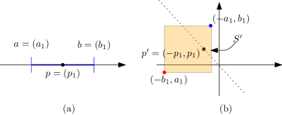
Figure 12: (a) A point $p$ in 1-D lying inside an interval $S=[a_{1},b_{1}]$, and (b) the transformation of $p$ into a point $p^{\prime}=(-p_{1},p_{1})$, and the transformation of $S$ into a square $S^{\prime}$ in 2-D.

Observation 1.

A point $p=(p_{1},\ldots,p_{d})$ lies inside $S$ if and only if $p^{\prime}=(-p_{1},\ldots,-p_{d},p_{1},\ldots,p_{d})$ lies inside $S^{\prime}$.

Proof.

Assume that $p$ lies inside $S$. Consider the $i$-th coordinate of $p^{\prime}$ with $i\leq d$. Since $b_{i}-a_{i}\leq\Delta$ implies that $-a_{i}-\Delta\leq-b_{i}$, we observe that $-a_{i}-\Delta\leq-b_{i}\leq-p_{i}\leq-a_{i}$. Therefore, for all $1\leq i\leq d$, we have $-a_{i}-\Delta\leq-p_{i}\leq-a_{i}$.

Now consider the $i$-th coordinate of $p^{\prime}$ with $i>d$. Since $b_{i}-a_{i}\leq\Delta$ implies that $b_{i}-\Delta\leq a_{i}$, we observe that $b_{i}-\Delta\leq a_{i}\leq p_{i}\leq b_{i}$. Therefore, for all $d+1\leq i\leq 2d$, we have $b_{i}-\Delta\leq p_{i}\leq b_{i}$. Thus, we claim that if a point $p$ lies inside $S$, then $p^{\prime}$ will lie inside $S^{\prime}$.

It is easy to prove the other direction. If $p$ lies outside $S$, then there is at least one coordinate (say $i$) in which either $p_{i}<a_{i}$ or $p_{i}>b_{i}$. If $p_{i}<a_{i}$, then $-p_{i}>-a_{i}$ and hence, $p^{\prime}$ lies outside $S^{\prime}$. On the other hand, if $p_{i}>b_{i}$, then again $p^{\prime}$ lies outside $S^{\prime}$. ∎

By a standard rank-space reduction we can assume that the corners of the hyperrectangles in $\mathcal{S}$ lie on the grid $[0,2m]^{d}$. After applying the above transformation, we note that the coordinates of the corners of the hypercubes in $\mathcal{S}^{\prime}$ will lie on the grid $[-4m,0]^{d}\times[-2m,2m]^{d}$: trivially, $\Delta+a_{i}\leq 4m$, and hence $-4m\leq-a_{i}-\Delta\leq-a_{i}\leq 0$. Also, $-2m\leq b_{i}-\Delta\leq b_{i}\leq 2m$. After performing a suitable shifting of the grid, we will assume that all corners of the hypercubes in $\mathcal{S}^{\prime}$ will lie on the grid $[0,4m]^{2d}$.

4.2 Constructing a bounded frequency set system.

We will now present a technique to select a set $\hat{\mathcal{S}}\subseteq\mathcal{S}^{\prime}$ with the following properties:

1. (Bounded frequency) Any point in $P^{\prime}$ lies inside $O(\log^{2d}m)$ hypercubes in $\hat{\mathcal{S}}$.

2. An $\alpha$-approximation dynamic set cover algorithm for $(P^{\prime},\hat{\mathcal{S}})$ implies an $O(\alpha\log^{2d-1}m)$-approximation dynamic set cover algorithm for $(P^{\prime},{\cal S}^{\prime})$.

3. The time taken to update the solution for the set system $(P^{\prime},\hat{\mathcal{S}})$ is $O(\log^{2d}m\cdot\log^{2}n)$.

4. The time taken to construct the set $\hat{\mathcal{S}}$ is $O(m\log^{2d}m)$.

4.2.1 Extended quad-tree for $2$-dimensional squares.

Given a set of squares $\mathcal{S}^{\prime}$, construct a 2-dimensional quad-tree $\mathbb{T}$ (as defined in Section 2), such that its root contains all the squares in $\mathcal{S}^{\prime}$. We assume for simplicity that no two input squares in $\mathcal{S}^{\prime}$ share a corner. Then, we can perturb the input points slightly so that no point $p\in P^{\prime}$ lies on any of the grid points of the quad-tree and each square still contains the same set of points as before. Consider a node $v\in\mathbb{T}$ and a square $S\in\mathcal{S}^{\prime}$. Let $C$ and $par(C)$ be the cell corresponding to node $v$ and the parent node of $v$, respectively. Let $\mathsf{proj}_{i}(C)$, $\mathsf{proj}_{i}(par(C))$ and $\mathsf{proj}_{i}(S)$ be the projection of $C$, $par(C)$ and $S$, respectively, on to the $i$-th dimension. Then $S$ is $i$-long at $v$ if and only if $\mathsf{proj}_{i}(C)\subseteq\mathsf{proj}_{i}(S)$ but $\mathsf{proj}_{i}(par(C))\not\subseteq\mathsf{proj}_{i}(S)$. See Figure 13(a). For all $u\in\mathbb{T}$, let $\mathcal{S}(u,i)\subseteq\mathcal{S}^{\prime}$ be the squares which are $i$-long at node $u$. Intuitively, these are squares that cover the edge of $C$ in the $i$-th dimension but do not cover any edge of $par(C)$ in the $i$-th dimension. Now, at each node of $\mathbb{T}$ we will construct two secondary structures as follows: the first structure is a $1$-dimensional quad-tree built on the projection of the squares in $\mathcal{S}(u,1)$ on to the second dimension , and the second structure is a $1$-dimensional quad-tree built on the projection of the squares in $\mathcal{S}(u,2)$ on to the first dimension.

In each secondary structure, an interval $I$ (corresponding to a square $S\in\mathcal{S}^{\prime}$) is assigned to a node $u$ if and only if $u$ is the node with the smallest depth (the root is at depth zero) where $I$ intersects either the left endpoint or the right endpoint of the cell $C_{u}$. See Figure 13(b). By this definition, any interval will be assigned to at most two nodes in the secondary structure.

Now we will use $\mathbb{T}$ to construct the geometric collection $\hat{\mathcal{S}}$. Let $V_{\text{sec}}$ be the set of nodes in all the secondary structures of $\mathbb{T}$. For any node $u\in V_{\text{sec}}$, among its assigned intervals which intersect the left (resp., right) endpoint of the cell $C_{u}$, identify the maximal interval $I_{\ell}$ (resp., $I_{r}$) , i.e., the interval which has maximum overlap with $C_{u}$. See Figure 13(c). We then do the following set of operations over all the nodes in $V_{\text{sec}}$: For a node $u\in V_{\text{sec}}$, denote by $S^{\prime}$ and $S^{\prime\prime}$ the corresponding squares for the assigned intervals $I_{\ell}$ and $I_{r}$, respectively. Further, let $w$ be the node in $\mathbb{T}$, on which the secondary structure of $u$ was constructed. Then, we include in $\hat{\mathcal{S}}$ the rectangles $S_{1}\cap C_{w}$ and $S_{2}\cap C_{w}$.

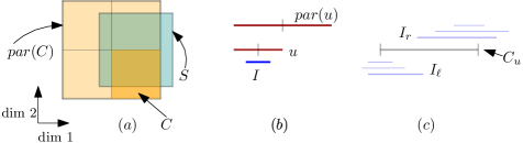
Figure 13: (a) A square $S$ which is $1$-long at node $v$ (corrs. cell $C$ is highlighted in darker orange), (b) $I$ is assigned to the two children of $v$, and (c) the maximal intervals $I_{\ell}$ and $I_{r}$ at $C_{v}$.

4.2.2 Extended quad-tree for $2d$-dimensional hypercubes.

In this section, we need a generalization of the quad-tree defined in Section 2. For $d^{\prime}>2$, a $d^{\prime}$-dimensional quad-tree is defined analogously to the the quad-tree defined in Section 2, where instead of four, each internal node will now have $2^{d^{\prime}}$ children. Assume by induction that we have defined how to construct the extended quad-tree for all dimensions less than or equal to $2d{-}1$. (The base case is the extended quad-tree built for $2$-dimensional squares). We define now how to construct the structure for $2d$-dimensional hypercubes. First construct the regular $2d$-dimensional quad-tree $\mathbb{T}$ for the set of hypercubes $\mathcal{S}^{\prime}$. Consider any node $v\in\mathbb{T}$. Generalizing the previous definition, for any $1\leq i\leq 2d$, a hypercube $S\in\mathcal{S}^{\prime}$ is defined to be $i$-long at node $v$ if and only if $\mathsf{proj}_{i}(C)\subseteq\mathsf{proj}_{i}(S)$, but $\mathsf{proj}_{i}(par(C))\not\subseteq\mathsf{proj}_{i}(S)$. For all $v\in\mathbb{T}$, let $\mathcal{S}(v,i)\subseteq\mathcal{S}^{\prime}$ be the hypercubes which are $i$-long at node $v$. Now, at each node of $\mathbb{T}$ we will construct $2d$ secondary structures as follows: for all $1\leq i\leq 2d$, the $i$-th secondary structure is a $(2d{-}1)$-dimensional extended quad-tree built on $\mathcal{S}(v,i)$ and all its $2d$ dimensions except the $i$-th dimension. Specifically, any hypercube $S\in\mathcal{S}(v,i)$ of the form $\ell_{1}\times\dots\times\ell_{i}\times\dots\times\ell_{2d}$ is projected to a $(2d{-}1)$-dimensional hypercube $\ell_{1}\times\dots\times\ell_{i-1}\times\ell_{i+1}\times\dots\times\ell_{2d}$. Let $\hat{\mathcal{S}}_{v}$ be the collection of the $(2d{-}1)$-dimensional hyperrectangles that are inductively picked for the secondary structure constructed at $v\in\mathbb{T}$ using the routine . Define the function $g$ which maps a $(2d{-}1)$-dimensional hyperrectangle picked as part of the collection $\hat{\mathcal{S}}_{v}$ (for a $v\in\mathbb{T}$) to its corresponding $2d$-dimensional hypercube $S\in\mathcal{S}^{\prime}$. We now define the collection of sets $\hat{\mathcal{S}}$ consisting of $2d$-dimensional hyperrectangles:

$$\hat{\mathcal{S}}\leftarrow\bigcup_{v\in\mathbb{T}}\left(\bigcup_{S^{\prime}\in\hat{\mathcal{S}}_{v}}(g(S^{\prime})\cap C_{v})\right).$$

Claim 6.

(Feasibility) Any point $p\in P^{\prime}$ is covered by at least one set in the collection $\hat{\mathcal{S}}$.

Proof.

We will prove the claim first for the case of 2-D squares. For any point $p\in P^{\prime}$, we know that at least one square $S\in\mathcal{S}^{\prime}$ covers it. By our assumption, $p$ is not on any of the grid points of the quad-tree. Then, we claim that $S$ is edge-covering for a cell $C_{v}$ such that $v$ is a leaf node and $C_{v}$ contains $p$. Then, by the definition of $i$-long, there exists an ancestor $u$ of $v$ in $\mathbb{T}$ (or possibly $v$ itself) such that $S$ is $i$-long for $C_{u}$, for some $i\in[2]$. This implies that $\hat{\mathcal{S}}$ consists of a (maximal) square $S^{\prime}$ such that $S^{\prime}\in\mathcal{S}(u,i)$ and $S^{\prime}\cap C_{u}\supseteq S\cap C_{u}$. Then, by our construction of the extended quad-tree, $S^{\prime}\cup C_{u}$ is part of the collection $\hat{\mathcal{S}}$. Hence, the claim holds for 2-D squares. Generalizing this idea, feasibility can be guaranteed for the case of $2d$-dimensional hypercubes for $d\geq 1$. ∎

Lemma 9.

(Bounded frequency) Any point in $P^{\prime}$ lies inside $O(\log^{2d}m)$ sets in $\hat{\mathcal{S}}$.

Proof.

For the extended quad-tree for $2$-dimensional squares, let $\tau(2)$ be the maximum number of sets in $\hat{\mathcal{S}}$ which contain a point $p=(p_{x},p_{y})\in P^{\prime}$. By properties of standard quad-tree, the number of nodes in the $2$-dimensional quad-tree whose corresponding cells contain $p$ is $O(\log m)$. At any such node, each of the secondary structures will have $O(\log m)$ nodes whose corresponding cells contain the projection of $p$ (either $p_{x}$ or $p_{y}$). At each cell in the secondary structure which contains $p$, we select at most two (maximal) hyperrectangles into $\hat{\mathcal{S}}$. Therefore, $\tau(2)=O(\log^{2}m)$.

In general, for an extended quad-tree for $d^{\prime}$-dimensional hypercubes, let $\tau(d^{\prime})$ be the maximum number of sets in $\hat{\mathcal{S}}$ that contain any given $d^{\prime}$-dimensional point. Since we construct $2d$ secondary structures at each node, we obtain the following recurrence:

$$\tau(2d)=O((2d)\log m)\cdot\tau(2d{-}1)=O(\log^{2d}m),$$

where the constant hidden by the big-$O$-notation depends on $d$. ∎

Lemma 10.

If there is an $\alpha$-approximation dynamic set cover algorithm for $(P^{\prime},\hat{\mathcal{S}})$ then there is an $O(\alpha\log^{2d-1}m)$-approximation dynamic set cover algorithm for $(P^{\prime},{\cal S}^{\prime})$.

Proof.

Let $\mathsf{OPT}$ and $\widehat{\mathsf{OPT}}$ be the size of the optimal set cover for $(P^{\prime},\mathcal{S}^{\prime})$ and $(P^{\prime},\hat{\mathcal{S}})$. For any hypercube $S$ in $\mathcal{S}^{\prime}$ we will show that there exists $O(\log^{2d-1}m)$ hyperrectangles in $\hat{\mathcal{S}}$ whose union will completely cover $S$. Therefore, $\widehat{\mathsf{OPT}}=\mathsf{OPT}\cdot O(\log^{2d-1}m)$. Note that for every set $S^{\prime}\in\hat{\mathcal{S}}$, there exists a corresponding hypercube $S\in\mathcal{S}^{\prime}$ which covers at least the set of points in $P^{\prime}$ that $S^{\prime}$ covers. For $(P^{\prime},\mathcal{S}^{\prime})$, an $\alpha$-approximation set cover for $(P^{\prime},\hat{\mathcal{S}})$ implies an approximation factor of:

$$\frac{b}{\mathsf{OPT}}=\frac{b\cdot O(\log^{2d-1}m)}{\widehat{\mathsf{OPT}}}=O(\alpha\log^{2d-1}m),$$

where the last equation follows from $b\leq\alpha\cdot\widehat{\mathsf{OPT}}$.

Finally, we establish the covering property. We will prove it via induction on the dimension size. As a base case, for squares in 2-D, let $\mu(2)$ be the number of sets needed in $\hat{\mathcal{S}}$ such that their union completely covers a square $S\in\mathcal{S}^{\prime}$. For any $S\in\mathcal{S}^{\prime}$, let $\mathsf{long}(S)$ be the set of nodes in $\mathbb{T}$ where $S$ is $1$-long. By standard properties of a quad-tree, we have (a) $|\mathsf{long}(S)|=O(\log m)$, and (b) $S\leftarrow\bigcup_{v\in\mathsf{long}(S)}(S\cap C_{v})$, where $C_{v}$ is the cell corresponding to $v$. Now consider any node $v\in\mathsf{long}(S)$. Let $I$ be the interval corresponding to $S$ in the secondary structure of $v$ built on $\mathcal{S}(v,1)$. Via our selection of maximal intervals at the secondary nodes, it is clear that there exist two maximal intervals which cover $I$. Therefore, $\mu(2)\leq 2\cdot|\mathsf{long}(S)|=O(\log m)$.

In general, let $\mu(2d)$ be the number of sets needed in $\hat{\mathcal{S}}$ such that their union completely covers a hypercube $S\in\mathcal{S}^{\prime}$. Then we claim that

$$\mu(2d)=O(2^{d}\log m)\times\mu(2d{-}1),$$

where $O(2^{d}\log m)$ is the number of nodes in $\mathbb{T}$ where $S$ is $1$-long. Solving the recurrence, we obtain $\mu(2d)=O(\log^{2d-1}m)$. ∎

4.3 The final algorithm

For the general dynamic set cover problem, Bhattacharya et al. [13] gave an $O(f)$-approximation algorithm with a worst-case update time of $O(f\log^{2}n)$. Recall that $f$ is the frequency of the set system. We will use their algorithm as a blackbox on the set system $(P^{\prime},\hat{\mathcal{S}})$. Let $\mathsf{ALG}$ be the sets reported by their algorithm. Then our algorithm will also report $\mathsf{ALG}$ as a set cover for $(P^{\prime},\mathcal{S}^{\prime})$. The solution is feasible since each set in $\hat{\mathcal{S}}$ belongs to $\mathcal{S}^{\prime}$ as well.

Lemma 11.

The approximation factor of our algorithm is $O(\log^{4d-1}m)$.

Proof.

For the set system $(P^{\prime},\hat{\mathcal{S}})$ the frequency $f=O(\log^{2d}m)$, and hence, the algorithm of [13] leads to an $O(\log^{2d}m)$ approximation for this set system. Using Lemma 10, this implies an approximation factor of $O(\log^{2d}m)\cdot O(\log^{2d-1}m)=O(\log^{4d-1}m)$ for the set system $(P^{\prime},\mathcal{S}^{\prime})$. ∎

Lemma 12.

The update time is $O(\log^{2d}m\cdot\log^{2}n)=O(\log^{2d+2}m)$.

Proof.

When a point is inserted or deleted, the $O(\log^{2d}m)$ sets in $\hat{\mathcal{S}}$ containing the point can be found in $O(\log^{2d}m)$ time by traversing the tree $\mathbb{T}$. The algorithm of [13] has an update time of $O(f\log^{2}n)=O(\log^{2d}m\cdot\log^{2}n)=O(\log^{2d+2}m)$. This is true since $d$-dimensional hypercubes have dual $VC$-dimension of $O(d)$ [32, 33] and hence, $O(\log n)=O(\log m)$. ∎

Lemma 13.

The time taken to construct the set $\hat{\mathcal{S}}$ is $O(m\log^{2d}m)$.

Proof.

Let $T(m,d)$ be the time taken to build the extended quad-tree on $m$ hypercubes in $d$ dimensions. As a base case, we first compute $T(m,1)$. Constructing the skeleton structure of the 1-dimensional quad-tree takes $O(m)$ time, since the endpoints of the intervals lie on the integer grid $[0,4m]$. Then “assigning” each interval to a node in this quad-tree takes $O(m\log m)$ time. For a node $v$ which is assigned $m_{v}$ intervals, finding the two maximal intervals takes $O(m_{v})$ time. Therefore, $T(m,1)=O(m\log m)+\sum_{v}O(m_{v})=O(m\log m)$.

Now consider the extended quad-tree on $m$ hypercubes in $2d$ dimensions. Again constructing the skeleton of the quad-tree takes only $O(m)$ time. For any $1\leq i\leq 2d$, finding the nodes in $\mathbb{T}$ where a hypercube is “$i$-long” takes $O(2^{2d}\log m)=O(\log m)$ time. Therefore,

$$T(m,2d) =O(m\log m)+\sum_{v}T(m_{v},2d-1)$$

$$=O(m\log m)+\sum_{v}m_{v}\log^{2d-1}m_{v}\qquad\qquad\text{(by induction)}$$

$$=O(m\log m)+\sum_{v}m_{v}\log^{2d-1}m$$

$$=O(m\log^{2d}m),\qquad\qquad\text{since, $\sum_{v}m_{v}=O(m\log m)$.}\qed$$

4.4 Weighted setting

We present an easy extension of our algorithm to the setting where each hyperrectangle $S\in\mathcal{S}$ has a weight $w_{S}\in[1,W]$. First, we round the weight of each set $S$ to the smallest power of two greater than or equal to $w_{S}$. This leads to $O(\log W)$ different weight classes. Next, for each weight class, we will build an extended quad-tree based on the hypercubes of that weight class after the reduction to the case of $2d$-dimensional hypercubes from $d$-dimensional hyperrectangles as shown in the previous section. Finally, let $\hat{\mathcal{S}}$ be the collection of (maximal) hypercubes obtained from all the $O(\log W)$ extended quad-trees. Run the dynamic set cover algorithm of Bhattacharya et al. [13] on $(P^{\prime},\hat{\mathcal{S}})$.

Lemma 14.

The approximation factor of the algorithm is $O(\log^{4d-1}m\cdot\log W)$.

Proof.

Consider the optimal solution for $(P^{\prime},\mathcal{S}^{\prime})$ and let $\mathsf{OPT}$ be the optimal weight. By rounding the weight of each set in the optimal solution, their total weight becomes at most $2\cdot\mathsf{OPT}$. Therefore, the weight of the optimal solution in the set system after rounding is at most $2\cdot\mathsf{OPT}$. Compared to the unweighted setting, now the frequency of the set system $(P^{\prime},\hat{\mathcal{S}})$ increases by a $O(\log W)$ factor. As a result, we obtain an approximation factor of $O(\log^{4d-1}m\cdot\log W)$. ∎

Lemma 15.

The update time of the algorithm is $O(\log^{2d}m\log^{3}(Wm))$.

Proof.

When a point is inserted or deleted, the $O(\log^{2d}m\log W)$ sets in $\hat{\mathcal{S}}$ containing the point can be found in $O(\log^{2d}m\log W)$ time by traversing the $O(\log W)$ extended quad-trees. The algorithm of [13] has an update time of $O(f\log^{2}Wn)=O(\log^{2d}m\log W\log^{2}Wn)=O(\log^{2d}m\log^{3}(Wm))$. ∎

Theorem 5.

There is an algorithm for weighted dynamic set cover for $d$-dimensional hyperrectangles with an approximation factor of $O(\log^{4d-1}m\cdot\log W)$ and an update time of $O(\log^{2d}m\cdot\log^{3}(Wm))$.

We also have the following corollary for dynamic set cover for $2d$-dimensional hypercubes where all the corners are integral and bounded in $[0,cm]^{2d}$ for some constant $c>0$.

Corollary 3.

There is an algorithm for weighted dynamic set cover for $2d$-dimensional hypercubes with an approximation factor of $O(\log^{4d-1}m\cdot\log W)$ and an update time of $O(\log^{2d}m\cdot\log^{3}(Wm))$, when all of their corners are integral and bounded in $[0,cm]^{2d}$ for a fixed $c>0$.

5 Dynamic hitting set for $d$-dimensional hyperrectangles

In this section we present a dynamic algorithm for hitting set for $d$-dimensional hyperrectangles. We will reduce the problem to an instance of dynamic set cover in $2d$-dimensional space and use the algorithm designed in the previous section (Theorem 3). Recall that $P$ is the set of points and $\mathcal{S}$ is the set of hyperrectangles. Assume that all the points of $P$ and the hyperrectangles in $\mathcal{S}$ lie in the box $[0,N]^{d}$. For all $p\in P$, we transform $p=(p_{1},\ldots,p_{d})$ to a $2d$-dimensional hypercube $\mathcal{S}(p)$ of side length $N$ and “lower-left” corner $p^{\prime}=(-p_{1},\ldots,-p_{d},p_{1},\ldots,p_{d})$. Let $\mathcal{S}(P)$ be the transformed hypercubes. Next, we transform each hyperrectangle, say $S\in\mathcal{S}$, with “lower-left” corner $a=(a_{1},\ldots,a_{d})$ and “top-right” corner $b=(b_{1},\ldots,b_{d})$ into a $2d$-dimensional point $P(S)=(-a_{1},\ldots,-a_{d},b_{1},\ldots,b_{d})$. Let $P(\mathcal{S})$ be the transformed points. See Figure 15.

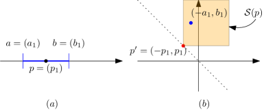
Figure 15: (a) A point $p$ in 1-D lying inside an interval $S=[a_{1},b_{1}]$, and (b) the transformation of $p$ into a square $\mathcal{S}(p)$, and transformation of $S$ into a point $(-a_{1},b_{1})$ in 2-D.

Lemma 16.

In $\mathbb{R}^{d}$ a point $p$ lies inside a hyperrectangle $S$, if and only if, in $\mathbb{R}^{2d}$ the hypercube $\mathcal{S}(p)$ contains the point $P(S)$.

Proof.

We define a point $q(q_{1},\ldots,q_{2d})$ to dominate another point $q^{\prime}(q^{\prime}_{1},\ldots,q^{\prime}_{2d})$ if and only if $q_{i}\geq q^{\prime}_{i}$, for all $1\leq i\leq 2d$. Assume that $p$ lies inside $S$. Then we have $p_{i}\geq a_{i}$ and $p_{i}\leq b_{i}$, for all $1\leq i\leq d$. This implies that $P(S)=(-a_{1},\ldots,-a_{d},b_{1},\ldots,b_{d})$ dominates the point $p^{\prime}(-p_{1},\ldots,-p_{d},p_{1},\ldots,p_{d})$, which is the lower-left corner of $\mathcal{S}(p)$.

The coordinates of the top-right corner of $\mathcal{S}(p)$ is $(-p_{1}+N,\ldots,-p_{d}+N,p_{1}+N,\ldots,p_{d}+N)$. For all $1\leq i\leq d$, since $N\geq p_{i}-a_{i}$, it implies that $-p_{i}+N\geq-a_{i}$. For all $1\leq i\leq d$, since $p_{i}+N\geq N\geq b_{i}$, it implies that $p_{i}+N\geq b_{i}$. This finally implies that that the top-right corner of $\mathcal{S}(p)$ dominates $P(S)$. Therefore, $\mathcal{S}(p)$ contains $P(S)$.

Assume that $p$ lies outside $S$. Then there exists a dimension $i$ such that $p_{i}<a_{i}$ or $p_{i}>b_{i}$. If $p_{i}<a_{i}$, then $-p_{i}>-a_{i}$, which implies that $P(S)$ cannot dominate the lower-left corner of $\mathcal{S}(p)$. If $p_{i}>b_{i}$, again $P(S)$ cannot dominate the lower-left corner of $\mathcal{S}(p)$. This implies that $P(S)$ lies outside $\mathcal{S}(p)$. ∎

We will use the above reduction to transform the points in $P$ into hypercubes in $\mathbb{R}^{2d}$ and transform the hyperrectangles in $\mathcal{S}$ into points in $\mathbb{R}^{2d}$. Therefore, the hitting set problem in $\mathbb{R}^{d}$ on hyperrectangles has been reduced to the set cover problem in $\mathbb{R}^{2d}$ on hypercubes. And with a similar rank-space reduction as mentioned in the previous section, all the points as well as the corners of the hypercubes in this instance have integral coordinates. Then, the set cover instance is answered using  Corollary 3. The correctness follows from Lemma 16. Noting that for $2d$-dimensional hypercubes, $O(\log n)=O(\log m)$, the performance of the algorithm is summarized below.

Theorem 6.

After performing a pre-processing step which takes $O(n\log^{2d}n)$ time, there is an algorithm for hitting set for $d$-dimensional hyperrectangles with an approximation factor of $O(\log^{4d-1}n)$ and an update time of $O(\log^{2d+2}n)$. In the weighted setting, the approximation factor is $O(\log^{4d-1}n\cdot\log W)$ and the update time is $O(\log^{2d}n\log^{3}(Wn))$.

6 Future work

In the first part of this work, we have studied online geometric set cover and hitting set for 2-D squares. This opens up an interesting line of work for the future. We state a few open problems:

1. As a natural extension of 2-D squares, is it possible to design a $o(\log n\log m)$-competitive algorithm for 3-D cubes? The techniques used in this paper for 2-D squares do not seem to extend to 3-D cubes. Another setting of interest here is when the geometric objects are 2-D disks. Can we obtain a $o(\log n\log m)$-competitive online set cover algorithm for them?

2. Design an online algorithm for set cover (resp., hitting set) for rectangles with competitive ratio $o(\log^{2}n)$ or show an almost matching lower bound of $\Omega\left(\frac{\log^{2}n}{\log\log n}\right)$ (which holds for the general case of online set cover [4])?

3. As a generalization of the above question, is it possible to obtain online algorithms for set cover and hitting set with competitive ratio $o(\log^{2}n)$ for set systems with “constant” VC-dimension.

4. For the weighted case of online set cover, even in unit squares, can we obtain algorithms with competitive ratio $o(\log n\log m)$?

5. Design an online algorithm for hitting set for squares with competitive ratio $O(\log n)$, and hence, improving our algorithm’s competitive ratio of $O(\log N)$ (where the corners of the squares are integral and contained in $[0,N)^{2}$).

In the second part of our work, we studied dynamic geometric set cover and hitting set for $d$-dimensional hyperrectangles. This line of work nicely brings together data structures, computational geometry, and approximation algorithms. We finish with a few open problems in the dynamic setting:

1. Improve the approximation factor for dynamic set cover for the case of 2-D rectangles. Specifically, is it possible to obtain an $O(\log n)$ approximation with polylogarithmic update time? In this setting the rectangles are fixed, but the points are dynamic.

2. For weighted dynamic set cover for the case of 2-D rectangles, is it possible to obtain approximation and update bounds independent of $W$ (where $W$ is the ratio of the weight of the highest weight rectangle to the lowest weight rectangle in the input)?

3. For the (fully) dynamic case of set cover studied in [3, 19, 20], can we obtain algorithms with sublinear update time and polylogarithmic approximation when the sets are rectangles (as originally asked in [20])?

Appendix A Online algorithms for interval set cover

In this section, we present a tight 2-competitive algorithm for the case of interval set cover.

In the algorithm, we start with an empty set cover. In each iteration, when a new point $p$ arrives, if it is covered then we do nothing. Otherwise, we select among the intervals covering $p$, the one with the rightmost right end-point and the one with the leftmost left end-point.

The correctness of the algorithm follows trivially, since for every new uncovered point we pick an interval covering it. We do not remove intervals from our solution at any later steps in the algorithm, and hence, all points are covered when the algorithm terminates.

Theorem 7.

There exists a 2-competitive algorithm for the online interval set cover problem.

Proof.

Consider an interval $I$ in the optimum solution $\mathsf{OPT}$. When the first uncovered point covered by it, arrives in the input, our algorithm picks two intervals and ensures that these two intervals cover all of $I$. Hence, for each interval in $\mathsf{OPT}$, we pick at most 2 intervals in our solution, giving us a 2-competitive solution. ∎

Theorem 8.

There is an instance of the set cover problem on intervals such that any online algorithm (without recourse) can at best be 2-competitive on this instance.

Proof.

Consider the given set of intervals to be $A:=[0,1],B:=[1,2],C:=[2,3],D:=[3,4]$. The first point to arrive is $p_{1}:=2$. If the algorithm picks two or more sets, then we are done as $\mathsf{OPT}$ is of size 1. Otherwise, to cover $p$, an algorithm can pick either interval $B$ or $C$. In the former case, the second point should be $p_{2}:=3$; and in the latter $p_{3}:=1$. We see that in both cases $\mathsf{OPT}$ is of size one, but an online algorithm is forced to pick two intervals. ∎

References

- [1] Amir Abboud, Raghavendra Addanki, Fabrizio Grandoni, Debmalya Panigrahi, and Barna Saha. Dynamic set cover: improved algorithms and lower bounds. In Proceedings of the 51st Annual ACM SIGACT Symposium on Theory of Computing (STOC), pages 114–125, 2019.
- [2] Pankaj K. Agarwal, Hsien-Chih Chang, Subhash Suri, Allen Xiao, and Jie Xue. Dynamic geometric set cover and hitting set. In 36th International Symposium on Computational Geometry, SoCG 2020, volume 164 of LIPIcs, pages 2:1–2:15. Schloss Dagstuhl - Leibniz-Zentrum für Informatik, 2020.
- [3] Pankaj K Agarwal, Hsien-Chih Chang, Subhash Suri, Allen Xiao, and Jie Xue. Dynamic geometric set cover and hitting set. arXiv preprint arXiv:2003.00202, 2020.
- [4] Noga Alon, Baruch Awerbuch, and Yossi Azar. The online set cover problem. In Proceedings of the thirty-fifth annual ACM symposium on Theory of computing (STOC), pages 100–105, 2003.
- [5] Boris Aronov, Esther Ezra, and Micha Sharir. Small-size eps-nets for axis-parallel rectangles and boxes. SIAM Journal on Computing, 39(7):3248–3282, 2010.
- [6] Sanjeev Arora. Polynomial time approximation schemes for euclidean traveling salesman and other geometric problems. Journal of the ACM (JACM), 45(5):753–782, 1998.
- [7] Sunil Arya, David M. Mount, Nathan S. Netanyahu, Ruth Silverman, and Angela Y. Wu. An optimal algorithm for approximate nearest neighbor searching fixed dimensions. Journal of the ACM (JACM), 45(6):891–923, 1998.
- [8] Sepehr Assadi and Shay Solomon. Fully dynamic set cover via hypergraph maximal matching: An optimal approximation through a local approach. In 29th Annual European Symposium on Algorithms, ESA 2021, page 8. Schloss Dagstuhl-Leibniz-Zentrum fur Informatik GmbH, Dagstuhl Publishing, 2021.
- [9] Mark de Berg, Marc van Kreveld, Mark Overmars, and Otfried Schwarzkopf. Computational geometry. In Computational geometry, pages 1–17. Springer, 1997.
- [10] Sayan Bhattacharya, Monika Henzinger, and Giuseppe F. Italiano. Deterministic fully dynamic data structures for vertex cover and matching. SIAM Journal on Computing, 47(3):859–887, 2018.
- [11] Sayan Bhattacharya, Monika Henzinger, and Giuseppe F. Italiano. Dynamic algorithms via the primal-dual method. Information and Computation, 261:219–239, 2018.
- [12] Sayan Bhattacharya, Monika Henzinger, and Danupon Nanongkai. A new deterministic algorithm for dynamic set cover. In 2019 IEEE 60th Annual Symposium on Foundations of Computer Science (FOCS), pages 406–423. IEEE, 2019.
- [13] Sayan Bhattacharya, Monika Henzinger, Danupon Nanongkai, and Xiaowei Wu. Dynamic set cover: Improved amortized and worst-case update time. In Proceedings of the 2021 ACM-SIAM Symposium on Discrete Algorithms (SODA), pages 2537–2549. SIAM, 2021.
- [14] Sujoy Bhore, Jean Cardinal, John Iacono, and Grigorios Koumoutsos. Dynamic geometric independent set. In Japan conference on Discrete and Computational Geometry, Graphs, and Games, 2021.
- [15] Marcin Bienkowski, Jarosław Byrka, Christian Coester, and Łukasz Jeż. Unbounded lower bound for k-server against weak adversaries. In Proceedings of the 52nd Annual ACM SIGACT Symposium on Theory of Computing (STOC), pages 1165–1169, 2020.
- [16] Niv Buchbinder and Joseph Naor. The design of competitive online algorithms via a primal-dual approach. Found. Trends Theor. Comput. Sci., 3(2-3):93–263, 2009.
- [17] Jean Cardinal, John Iacono, and Grigorios Koumoutsos. Worst-case efficient dynamic geometric independent set. In 29th Annual European Symposium on Algorithms (ESA 2021). Schloss Dagstuhl-Leibniz-Zentrum für Informatik, 2021.
- [18] Timothy M. Chan, Elyot Grant, Jochen Könemann, and Malcolm Sharpe. Weighted capacitated, priority, and geometric set cover via improved quasi-uniform sampling. In Proceedings of the twenty-third annual ACM-SIAM symposium on Discrete Algorithms (SODA), pages 1576–1585. SIAM, 2012.
- [19] Timothy M. Chan and Qizheng He. More dynamic data structures for geometric set cover with sublinear update time. In 37th International Symposium on Computational Geometry (SoCG 2021). Schloss Dagstuhl-Leibniz-Zentrum für Informatik, 2021.
- [20] Timothy M. Chan, Qizheng He, Subhash Suri, and Jie Xue. Dynamic geometric set cover, revisited. In Proceedings of the 2022 Annual ACM-SIAM Symposium on Discrete Algorithms (SODA), pages 3496–3528. SIAM, 2022.
- [21] Kenneth L. Clarkson and Kasturi Varadarajan. Improved approximation algorithms for geometric set cover. In Proceedings of the twenty-first annual symposium on Computational geometry (SoCG), pages 135–141, 2005.
- [22] Justin Dallant and John Iacono. Conditional lower bounds for dynamic geometric measure problems. arXiv preprint arXiv:2112.10095, 2021.
- [23] Guy Even and Shakhar Smorodinsky. Hitting sets online and vertex ranking. In Algorithms - ESA 2011 - 19th Annual European Symposium, volume 6942 of Lecture Notes in Computer Science, pages 347–357. Springer, 2011.
- [24] Anupam Gupta, Gregory Kehne, and Roie Levin. Random order online set cover is as easy as offline. In 2021 IEEE 62nd Annual Symposium on Foundations of Computer Science (FOCS), pages 1253–1264. IEEE, 2022.
- [25] Anupam Gupta, Ravishankar Krishnaswamy, Amit Kumar, and Debmalya Panigrahi. Online and dynamic algorithms for set cover. In Proceedings of the 49th Annual ACM SIGACT Symposium on Theory of Computing (STOC), pages 537–550, 2017.
- [26] Anupam Gupta and Roie Levin. Fully-dynamic submodular cover with bounded recourse. In 2020 IEEE 61st Annual Symposium on Foundations of Computer Science (FOCS), pages 1147–1157. IEEE, 2020.
- [27] Anupam Gupta and Roie Levin. The online submodular cover problem. In Proceedings of the Fourteenth Annual ACM-SIAM Symposium on Discrete Algorithms (SODA), pages 1525–1537. SIAM, 2020.
- [28] Sariel Har-Peled and Mira Lee. Weighted geometric set cover problems revisited. Journal of Computational Geometry, 3(1):65–85, 2012.
- [29] Monika Henzinger, Stefan Neumann, and Andreas Wiese. Dynamic approximate maximum independent set of intervals, hypercubes and hyperrectangles. In 36th International Symposium on Computational Geometry, SoCG 2020, volume 164 of LIPIcs, pages 51:1–51:14. Schloss Dagstuhl - Leibniz-Zentrum für Informatik, 2020.
- [30] Nabil H. Mustafa, Rajiv Raman, and Saurabh Ray. Settling the apx-hardness status for geometric set cover. In 2014 IEEE 55th Annual Symposium on Foundations of Computer Science (FOCS), pages 541–550. IEEE, 2014.
- [31] Nabil H. Mustafa and Saurabh Ray. PTAS for geometric hitting set problems via local search. In Proceedings of the 25th ACM Symposium on Computational Geometry (SoCG), pages 17–22. ACM, 2009.
- [32] Norbert Sauer. On the density of families of sets. Journal of Combinatorial Theory, Series A, 13(1):145–147, 1972.
- [33] Saharon Shelah. A combinatorial problem; stability and order for models and theories in infinitary languages. Pacific Journal of Mathematics, 41(1):247–261, 1972.
- [34] Kasturi Varadarajan. Weighted geometric set cover via quasi-uniform sampling. In Proceedings of the forty-second ACM symposium on Theory of computing (STOC), pages 641–648, 2010.