LDMVFI: Video Frame Interpolation with Latent Diffusion Models

Abstract

Existing works on video frame interpolation (VFI) mostly employ deep neural networks that are trained by minimizing the L1, L2, or deep feature space distance (e.g. VGG loss) between their outputs and ground-truth frames. However, recent works have shown that these metrics are poor indicators of perceptual VFI quality. Towards developing perceptually-oriented VFI methods, in this work we propose latent diffusion model-based VFI, LDMVFI. This approaches the VFI problem from a generative perspective by formulating it as a conditional generation problem. As the first effort to address VFI using latent diffusion models, we rigorously benchmark our method on common test sets used in the existing VFI literature. Our quantitative experiments and user study indicate that LDMVFI is able to interpolate video content with favorable perceptual quality compared to the state of the art, even in the high-resolution regime. Our code is available at https://github.com/danier97/LDMVFI.

1 Introduction

Video frame interpolation (VFI) aims to generate intermediate frames between two existing consecutive video frames. It is commonly used to synthetically increase frame rate, e.g., to produce jitter-free slow-motion content (Jiang et al. 2018). VFI has also been used in video compression (Wu, Singhal, and Krahenbuhl 2018), view synthesis (Flynn et al. 2016), medical imaging (Karargyris and Bourbakis 2010) and animation production (Siyao et al. 2021).

Existing VFI methods (Jiang et al. 2018; Xue et al. 2019; Lee et al. 2020; Niklaus and Liu 2020; Kalluri et al. 2023) are mostly based on deep neural networks. These deep models differ in architectural designs and motion modeling approaches, but are mostly trained to minimize the L1, L2, or VGG (Simonyan and Zisserman 2015) feature distance between their outputs and the ground-truth intermediate frames. However, recent works (Men et al. 2020; Danier, Zhang, and Bull 2022d) have shown that these optimization objectives are not indicative of the perceptual quality of interpolated videos, as they correlate poorly with human judgments. As a result, it has been reported (Danier, Zhang, and Bull 2022d) that existing methods, while achieving high PSNR values, tend to under-perform perceptually, especially under challenging scenarios involving dynamic textures with complex motion.

Figure 1: Overview of the diffusion processes in LDMVFI. The encoder and decoder enable projection between image and latent spaces, and the diffusion processes take place in the latent space.

A potential approach to improve the perceptual performance of VFI methods is to develop more accurate perceptual metrics for training VFI models, and this is the focus of another research area, namely Video Quality Assessment (Saha et al. 2023). In this work, instead of relying on particular metrics, we explore a new direction for perception-oriented VFI based on diffusion models (Ho, Jain, and Abbeel 2020; Rombach et al. 2022). Diffusion models have recently exhibited remarkable performance in generating realistic, perceptually-optimized images and videos, reportedly outperforming other generative models including GANs and VAEs (Dhariwal and Nichol 2021; Ho et al. 2022). However, despite their ability to synthesize high-fidelity visual content, the application of diffusion models for VFI has not been fully investigated.

In the above context, we propose a latent diffusion model for video frame interpolation (LDMVFI), where VFI is formulated as a conditional image generation problem. Specifically, we adopt the recently proposed latent diffusion models (Rombach et al. 2022) (LDMs) within a framework comprising an autoencoding model that projects images into a latent space, and a denoising U-Net which performs reverse diffusion process in that latent space. To better adapt LDMs to VFI, we devise VFI-specific components, notably a novel vector quantization-based VFI-autoencoding model, VQ-FIGAN, with which our method shows superior performance over vanilla LDMs.

Despite the paradigmatic shift from the mainstream VFI methods, we adhere to the commonly adopted VFI benchmarking protocol and evaluate the proposed method on various VFI test sets, covering both low and high resolution content (up to 4K). Our results demonstrate that LDMVFI performs favorably against the state of the art in terms of three perceptual metrics (Zhang et al. 2018; Danier, Zhang, and Bull 2022b; Heusel et al. 2017). We also conducted a user study to collect subjective judgments on the quality of full HD videos interpolated by our method benchmarked against several competitive counterparts; this further confirms the favorable perceptual performance of LDMVFI.

To the best of our knowledge, this work is the first to address VFI as a conditional generation problem using latent diffusion models, and the first to demonstrate the potential of the new paradigm for perception-oriented VFI. Our contributions are summarized below.

• We present LDMVFI, a latent diffusion-based method that leverages the high-fidelity image synthesis ability of diffusion models to perform VFI.

• We introduce novel VFI-specific components into LDMs, including a vector-quantized autoencoding model, VQ-FIGAN, which further enhances VFI performance.

• We demonstrate, through quantitative and qualitative experiments, that the proposed method performs favorably against the state of the art.

2 Relate Work

Video Frame Interpolation.

Existing VFI approaches are mostly based on deep learning, and can be generally categorized as flow-based or kernel-based. Flow-based methods rely on optical flow estimation to generate interpolated frames. To obtain the optical flow from input frames to the non-existent middle frame (or the other way around), some methods (Jiang et al. 2018; Niklaus and Liu 2018, 2020; Sim, Oh, and Kim 2021) assume certain motion types to infer the intermediate optical flows using the flows between two input frames, while others (Liu et al. 2017; Xue et al. 2019; Park et al. 2020; Park, Lee, and Kim 2021; Lu et al. 2022b; Kong et al. 2022) directly estimate the intermediate flows. On the other hand, kernel-based methods argue that optical flows can be unreliable in dynamic texture scenes, so they predict locally adaptive convolution kernels to synthesize output pixels, allowing more flexible many-to-one mapping. While earlier methods (Niklaus, Mai, and Liu 2017) in this class predict fixed-size kernels, more recent ones (Lee et al. 2020; Ding et al. 2021; Cheng and Chen 2020, 2022; Danier, Zhang, and Bull 2022a) tend to adopt deformable convolution (Dai et al. 2017) kernels. Other than these two classes, there are also attempts to combine flows and kernels (Bao et al. 2021; Danier, Zhang, and Bull 2022c), and to perform end-to-end frame synthesis (Choi et al. 2020; Kalluri et al. 2023).

It is noted that the above methods are trained by optimizing PSNR-oriented loss functions, i.e., the L1/L2 distance between the model outputs and the ground-truth frames. To improve perceptual performance, some existing methods (Niklaus and Liu 2018, 2020) use the VGG (Simonyan and Zisserman 2015) feature-based loss in combination with the L1 loss. However, it has been previously reported (Danier, Zhang, and Bull 2022d) that these distances do not fully reflect the perceptual quality of interpolated videos, exhibiting poor correlation performance with subjective ground truth. As a result, it has been observed (Danier, Zhang, and Bull 2022d) that some state-of-the-art methods show unsatisfactory perceptual performance, especially on dynamic textures with complex motions.

Diffusion Models.

Recently, diffusion models (DMs) (Ho, Jain, and Abbeel 2020; Rombach et al. 2022) have demonstrated remarkable performance in synthesizing high-fidelity images and videos. In their original form (Ho, Jain, and Abbeel 2020), DMs generate new images by progressively denoising a Gaussian noise image; the process corresponds to the reverse of a Markov chain that gradually adds noise to a clean image. DMs have been reported to offer superior performance (Dhariwal and Nichol 2021; Ho et al. 2022) compared to GANs (Goodfellow et al. 2020) and VAEs (Kingma and Welling 2014) in image generation tasks. The only previous application of DMs on VFI is (Voleti, Jolicoeur-Martineau, and Pal 2022), but this work focused on low-resolution images and the model lacked any VFI-specific innovations, showing limited interpolation performance. The recently proposed latent diffusion models (LDMs) have demonstrated strong ability to synthesize high-resolution images by performing diffusion processes in latent space. However, we observe that LDMs have not previously been exploited for VFI.

3 Proposed Method: LDMVFI

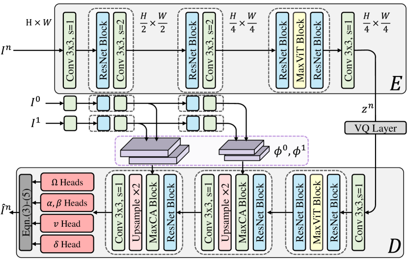
Given two consecutive frames $I^{0},I^{1}$ from a video, VFI aims to generate the non-existent intermediate frame $I^{n}$ where $n=0.5$ for $\times$2 upsampling. Approaching VFI from a generative perspective, our goal is to learn a parametric approximation of the conditional distribution $p(I^{n}|I^{0},I^{1})$ using a dataset $\mathcal{D}=\{I^{0}_{s},I^{n}_{s},I^{1}_{s}\}_{s=1}^{S}$. To achieve this, we adopt the latent diffusion models (Rombach et al. 2022) to perform conditional generation for VFI. The proposed LDMVFI contains two main components: (i) a VFI-specific autoencoding model, VQ-FIGAN, that projects frames into a latent space, and reconstructs the target frame from the latent encoding; (ii) a denoising U-Net that performs reverse diffusion process in the latent space for conditional image generation. Figure 1 shows the overview of the LDMVFI.

Figure 2: The architecture of the VFI autoencoding model, VQ-FIGAN. It differs from the original VQGAN (Esser, Rombach, and Ommer 2021) in three aspects: (i) the use of features extracted by the encoder from neighboring frames during the decoding via MaxViT-based cross attention; (ii) use of more efficient MaxViT block instead of the vanilla self-attention; (iii) frame synthesis via adaptive deformable convolution. The kernel ($\Omega$), offset ($\alpha,\beta$), visibility ($v$) and residual ($\delta$) heads contain 3$\times${conv3x3, ReLU}.

3.1 Latent Diffusion Models

Latent diffusion models (LDMs) (Rombach et al. 2022) are built upon the denoising diffusion probabilistic models (Ho, Jain, and Abbeel 2020) (referred to as diffusion models hereafter), which are a class of generative models that learns a data distribution $p(x)$ by learning the reverse process of a pre-defined Markov Chain of length $T$ (i.e. the forward process) that gradually adds Gaussian noise to the data. Specifically, a time-conditioned neural network $\epsilon_{\theta}(x_{t},t)$ is trained to denoise the data at step $t=1,\dots,T$ with the objective

$$\mathcal{L}_{\mathrm{DM}}=\mathbb{E}_{x_{0},\epsilon\sim\mathcal{N}(\mathbf{0},\mathbf{I}),t\sim\mathcal{U}(1,T)}\big{[}\left\lVert\epsilon-\epsilon_{\theta}(x_{t},t)\right\rVert^{2}\big{]},$$ (1)

where $x_{t}$ is sampled from the forward diffusion process and $\mathcal{U}(1,T)$ denotes uniform distribution over $\{1,\dots,T\}$. This corresponds to a reweighted version of the variational lower bound on $\log p(x)$. More details of diffusion processes and the loss are provided in Appendix A.

To sample new images, one can start from a Gaussian noise and gradually denoise it using the denoising network $\epsilon_{\theta}$. Under the conditional generation setting, we can condition $\epsilon_{\theta}$ on an additional input $y$, which can denote the two input frames in the context of VFI.

Latent diffusion models contain an image encoder $E:x\mapsto z$ that encodes an image $x$ into a lower-dimensional latent representation $z$, and a decoder $D:z\mapsto x$ that reconstructs the image $x$. The forward and reverse diffusion processes then happen in the latent space, and the training objective for learning the reverse diffusion process becomes

$$\mathcal{L}_{\mathrm{LDM}}=\mathbb{E}_{E(x_{0}),\epsilon\sim\mathcal{N}(\mathbf{0},\mathbf{I}),t\sim\mathcal{U}(1,T)}\big{[}\left\lVert\epsilon-\epsilon_{\theta}(z_{t},t)\right\rVert^{2}\big{]}.$$ (2)

By projecting images into a compact latent space, LDMs allow the diffusion process to concentrate on the semantically important portions of the data and enable more computationally efficient sampling process.

3.2 Autoencoding with VQ-FIGAN

In the original form of LDMs, the autoencoding model $\{E,D\}$ is considered as a perceptual image codec. Its design purpose is to project images into efficient latent representations where high-frequency details are removed during encoding and recovered in the decoding. However, in the context of VFI, such information is likely to affect the perceived quality of the interpolated videos, so the limited reconstruction ability of the decoder can negatively impact the VFI performance. To enhance high-frequency detail recovering, we propose a VFI-specific autoencoding model: VQ-FIGAN, which is illustrated in Figure 2. While the backbone model is similar to the original VQGAN (Esser, Rombach, and Ommer 2021) used in (Rombach et al. 2022), there are three major differences.

Firstly, we take advantage of a property of the VFI task - that the neighboring frames are available during inference, in order to design a frame-aided decoder. Specifically, given the ground-truth target frame $I^{n}\in\mathbb{R}^{H\times W\times 3}$, the encoder $E$ produces the latent encoding $z^{n}=E(I^{n})$, where $z^{n}\in\mathbb{R}^{\frac{H}{f}\times\frac{W}{f}\times 3}$, and $f$ is a hyper-parameter (Figure 2 shows the case for $f=4$). Then, the decoder $D$ outputs a reconstructed frame, $\hat{I}^{n}$, taking input $z^{n}$, as well as the feature pyramids, $\phi^{0},\phi^{1}$, extracted by $E$ from two neighboring frames, $I^{0},I^{1}$. During decoding, these feature pyramids are fused with the decoded features from $z^{n}$ at multiple layers using the MaxCA blocks, which are newly designed MaxViT (Tu et al. 2022)-based Cross Attention blocks, where the query embeddings for the attention mechanism are generated using decoded features from $z^{n}$, and the key and value embeddings are obtained from $\phi^{0},\phi^{1}$.

Secondly, we notice the original VQGAN uses the full self-attention (Vaswani et al. 2017) as in the vision transformer (Dosovitskiy et al. 2021), which can be computationally heavy (quadratic complexity) and memory-intensive, especially when the image resolution is high. For more efficient inference on high-resolution (e.g. full HD) videos, we employ the recently proposed MaxViT block (Tu et al. 2022) to perform self-attention. The multi-axis self-attention layer in the MaxViT block combines windowed attention and dilated grid attention to perform both local and global operations, while achieving linear complexity with respect to the input size.

Thirdly, instead of having the decoder directly output the reconstructed image $\hat{I}^{n}$, the proposed VQ-FIGAN outputs the deformable convolution-based interpolation kernels (Dai et al. 2017; Lee et al. 2020; Cheng and Chen 2020) to enhance VFI performance. Specifically, given that $H,W$ are the frame height and width, the output of the decoder network contains parameters of the locally adaptive deformable convolution kernels of size $K\times K$: $\{\Omega^{\tau},\alpha^{\tau},\beta^{\tau}\}$ where $\tau=0,1$ indexes the input frames. Here $\Omega\in[0,1]^{H\times W\times K\times K}$ contains the weights of the kernels, and $\alpha,\beta\in\mathbb{R}^{H\times W\times K\times K}$ are their spatial offsets (horizontal and vertical respectively). The decoder also outputs a visibility map $v\in[0,1]^{H\times W}$ to account for occlusion (Jiang et al. 2018), and a residual map $\delta\in\mathbb{R}^{H\times W}$ to further enhance VFI performance (Cheng and Chen 2022). To generate the interpolated frame, firstly locally adaptive deformable convolutions are performed for each input frame $\{I^{\tau}\}_{\tau=0,1}$:

$$I^{n\tau}(h,w)=\sum_{i=1}^{K}\sum_{j=1}^{K}\Omega^{\tau}_{h,w}(i,j)\cdot P^{\tau}_{h,w}(i,j),$$ (3)

$$P^{\tau}_{h,w}(i,j)=I^{\tau}(h+\alpha^{\tau}_{h,w}(i,j),w+\beta^{\tau}_{h,w}(i,j)),$$ (4)

in which $I^{n\tau}$ denotes the result obtained from $I^{\tau}$, and $P^{\tau}_{h,w}$ is the patch sampled from $I^{\tau}$ for output location $(h,w)$. These intermediate results are then combined using the visibility and residual maps:

$$\hat{I}^{n}=v\cdot I^{n0}+(1-v)\cdot I^{n1}+\delta.$$ (5)

We adopt the separable deformable convolution implementation in (Cheng and Chen 2020) which exploits separability properties of kernels (Rigamonti et al. 2013) to reduce memory requirements while maintaining VFI performance.

Training VQ-FIGAN.

We follow the original training settings of VQGAN in (Esser, Rombach, and Ommer 2021; Rombach et al. 2022), where the loss function consists of an LPIPS-based (Zhang et al. 2018) perceptual loss, a patch-based adversarial loss (Isola et al. 2017) and a latent regularization term based on a vector quantization (VQ) layer (Van Den Oord, Vinyals et al. 2017). We refer the readers to (Esser, Rombach, and Ommer 2021) for the details.

3.3 Conditional Generation with LDM

The trained VQ-FIGAN allows us to access a compact latent space in which we perform forward diffusion by gradually adding Gaussian noise to the latent $z^{n}$ of the target frame $I^{n}$ according to a pre-defined noise schedule, and learn the reverse (denoising) process to perform conditional generation. To this end, we adopt the noise-prediction parameterization (Ho, Jain, and Abbeel 2020) of DMs and train a denoising U-Net by minimizing the re-weighted variational lower bound on the conditional log-likelihood $\log p_{\theta}(z^{n}|z^{0},z^{1})$ where $z^{0},z^{1}$ are the latent encodings of the two input frames.

Training.

Specifically, the denoising U-Net $\epsilon_{\theta}$ takes as input the “noisy” latent encoding $z^{n}_{t}$ for the target frame $I^{n}$ (sampled from the $t$-th step in the forward diffusion process of length $T$), the diffusion step $t$, as well as the conditioning latents $z^{0},z^{1}$ for the input frames $I^{0},I^{1}$. It is trained to predict the noise added to $z^{n}$ at each time step $t$ by minimizing

$$\mathcal{L}=\mathbb{E}_{z^{n},z^{0},z^{1},\epsilon\sim\mathcal{N}(\mathbf{0},\mathbf{I}),t}\big{[}\left\lVert\epsilon-\epsilon_{\theta}(z^{n}_{t},t,z^{0},z^{1})\right\rVert^{2}\big{]},$$ (6)

where $t\sim\mathcal{U}(1,T)$. The derivation and full details of the training procedure of $\epsilon_{\theta}$ are provide in Appendix B. Intuitively, the training is performed by alternately adding a random Gaussian noise to $z^{n}$ according to a pre-defined noising schedule, and having the network $\epsilon_{\theta}$ predict the noise added given the step $t$, conditioning on $z^{0},z^{1}$.

Inference.

To interpolate $\hat{I}^{n}$ from $I^{0},I^{1}$, we start by sampling a Gaussian noise $z^{n}_{T}$ in the latent space, and perform $T$ steps of denoising until we obtain $z^{n}_{0}$. Within each step, firstly the network $\epsilon_{\theta}$ predicts the noise $\hat{\epsilon}$. Then $z^{n}_{t-1}$ is calculated using $\hat{\epsilon}$ and relevant parameters of the pre-defined forward process. Finally, the decoder $D$ produces the interpolated frame from the denoised latent $z^{n}_{0}$, with the help of feature pyramids $\phi^{0},\phi^{1}$ extracted by the encoder $E$ from $I^{0},I^{1}$. Full details are provided in the Appendix B.

Network Architecture.

We employ the time-conditioned U-Net as in (Rombach et al. 2022) for $\epsilon_{\theta}$, but with one modification: all the vanilla self-attention blocks (Vaswani et al. 2017) are replaced with the aforementioned MaxViT blocks (Tu et al. 2022) for computational efficiency. The conditioning mechanism for the U-Net is concatenation of $z^{n}_{t}$ and $z^{0},z^{1}$ at the input. The architecture is detailed in Appendix D.

4 Experimental setup

Implementation Details.

We set the downsampling factor of VQ-FIGAN to $f=32$, by repeating the ResNetBlock+Conv3x3 layer in the encoder and the corresponding layer in the decoder three times (see Figure 2). The size of the kernels output by the decoder is $K=5$. Regarding the diffusion processes, following (Rombach et al. 2022), we adopt a linear noise schedule and a codebook size of 8192 for vector quantization in VQ-FIGAN. We sample from all diffusion models with the DDIM (Song, Meng, and Ermon 2021) sampler for 200 steps (details provided in Appendix C). We also follow (Rombach et al. 2022) to train the VQ-FIGAN using the ADAM (Kingma and Ba 2015) optimizer and the denoising U-Net using the Adam-W optimizer (Loshchilov and Hutter 2019), with the initial learning rates set to $10^{-5}$ and $10^{-6}$ respectively. All models were trained until convergence, which corresponds to around 70 epochs for VQ-FIGAN, and around 60 epochs for the U-Net. NVIDIA RTX 3090 GPUs were used for all training and evaluation.

	Middlebury			UCF-101			DAVIS			VFITex			RT (sec)	#P (M)
	LPIPS$\downarrow$	FloLPIPS$\downarrow$	FID$\downarrow$	LPIPS$\downarrow$	FloLPIPS$\downarrow$	FID$\downarrow$	LPIPS$\downarrow$	FloLPIPS$\downarrow$	FID$\downarrow$	LPIPS$\downarrow$	FloLPIPS$\downarrow$	FID$\downarrow$
BMBC	0.023	0.037	12.974	0.034	0.045	33.171	0.125	0.185	15.354	0.220	0.282	50.393	0.51	11.0
AdaCoF	0.031	0.052	15.633	0.034	0.046	32.783	0.148	0.198	17.194	0.204	0.273	42.255	0.01	21.8
CDFI	0.022	0.043	12.224	0.036	0.049	33.742	0.157	0.211	18.098	0.218	0.286	43.498	0.02	5.0
XVFI	0.036	0.070	16.959	0.038	0.050	33.868	0.129	0.185	16.163	0.188	0.255	42.055	0.08	5.6
ABME	0.027	0.040	11.393	0.058	0.069	37.066	0.151	0.209	16.931	0.254	0.341	53.317	0.27	18.1
IFRNet	0.020	0.039	12.256	0.032	0.044	28.803	0.114	0.170	14.227	0.200	0.273	42.266	0.02	5.0
VFIformer	0.031	0.065	15.634	0.039	0.051	34.112	0.191	0.242	21.702	OOM	OOM	OOM	1.74	5.0
ST-MFNet	N/A	N/A	N/A	0.036	0.049	34.475	0.125	0.181	15.626	0.216	0.276	41.971	0.14	21.0
FLAVR	N/A	N/A	N/A	0.035	0.046	31.449	0.209	0.248	22.663	0.234	0.295	56.690	0.02	42.1
MCVD	0.123	0.138	41.053	0.155	0.169	102.054	0.247	0.293	28.002	OOM	OOM	OOM	52.55	27.3
LDMVFI	0.019	0.044	16.167	0.026	0.035	26.301	0.107	0.153	12.554	0.150	0.207	32.316	8.48	439.0

Table 1: Quantitative comparison of LDMVFI ($f=32$) and 10 tested methods on Middlebury, UCF-101, DAVIS and VFITex. Note ST-MFNet and FLAVR require four input frames so cannot be evaluated on Middlebury dataset which contains frame triplets. For each column, the best result is boldfaced. The last two columns show the average run time (RT) needed to to interpolate one 480p frame, and the number of parameters (#P) in each model.

	SNU-FILM-Easy			SNU-FILM-Medium			SNU-FILM-Hard			SNU-FILM-Extreme
	LPIPS$\downarrow$	FloLPIPS$\downarrow$	FID$\downarrow$	LPIPS$\downarrow$	FloLPIPS$\downarrow$	FID$\downarrow$	LPIPS$\downarrow$	FloLPIPS$\downarrow$	FID$\downarrow$	LPIPS$\downarrow$	FloLPIPS$\downarrow$	FID$\downarrow$
BMBC	0.020	0.031	6.162	0.034	0.059	12.272	0.068	0.118	25.773	0.145	0.237	49.519
AdaCoF	0.021	0.033	6.587	0.039	0.066	14.173	0.080	0.131	27.982	0.152	0.234	52.848
CDFI	0.019	0.031	6.133	0.036	0.066	12.906	0.081	0.141	29.087	0.163	0.255	53.916
XVFI	0.022	0.037	7.401	0.039	0.072	16.000	0.075	0.138	29.483	0.142	0.233	54.449
ABME	0.022	0.034	6.363	0.042	0.076	15.159	0.092	0.168	34.236	0.182	0.300	63.561
IFRNet	0.019	0.030	5.939	0.033	0.058	12.084	0.065	0.122	25.436	0.136	0.229	50.047
ST-MFNet	0.019	0.031	5.973	0.036	0.061	11.716	0.073	0.123	25.512	0.148	0.238	53.563
FLAVR	0.022	0.034	6.320	0.049	0.077	15.006	0.112	0.169	34.746	0.217	0.303	72.673
MCVD	0.199	0.230	32.246	0.213	0.243	37.474	0.250	0.292	51.529	0.320	0.385	83.156
LDMVFI	0.014	0.024	5.752	0.028	0.053	12.485	0.060	0.114	26.520	0.123	0.204	47.042

Table 2: Quantitative comparison results on SNU-FILM (note VFIformer is not included because the GPU goes out of memory).

Training Dataset.

We utilize the most commonly used training set in VFI, Vimeo90k (Xue et al. 2019). However, previous works (Sim, Oh, and Kim 2021) have discussed the limited range of motion magnitudes and the diversity of Vimeo90k. To better test the learning capability and performance of VFI methods on a wider range of scenarios, we follow (Danier, Zhang, and Bull 2022c) to additionally incorporate samples from the BVI-DVC dataset (Ma, Zhang, and Bull 2021). The final training set thus comprises 64612 and 17600 frame triplets (using only the three frames in the center) from Vimeo90k-septuplets and BVI-DVC respectively. For data augmentation, we randomly crop $256\times 256$ patches and perform random flipping and temporal order reversing. It is noted that most existing works use only Vimeo90k-triplet for training, so for reference, we also provide evaluation results for LDMVFI trained on this dataset alone (see Appendix F).

Figure 3: Visual examples of frames interpolated by the state-of-the-art methods and the proposed LDMVFI. Under large and complex motions, our method preserves the most high-frequency details, delivering superior perceptual quality.

Figure 4: Results of the user study in terms of preference ratio. Error bar reflects the standard error over test sequences.

Test Datasets.

We evaluate models on the most commonly used VFI benchmarks, including Middlebury (Baker et al. 2011), UCF-101 (Soomro, Zamir, and Shah 2012), DAVIS (Perazzi et al. 2016), SNU-FILM (Choi et al. 2020), and VFITex (Danier, Zhang, and Bull 2022c). These test sets cover resolutions from $225\times 225$ up to 4K, and various levels of VFI difficulties. To further assess the perceptual performance, we perform user study using the BVI-HFR (Mackin, Zhang, and Bull 2018) dataset which covers a wide range of texture and motion types.

Evaluation Methods.

As the main focus of this work is on improving the perceptual quality of interpolated content, we adopt a perceptual image quality metric LPIPS (Zhang et al. 2018), and a bespoke VFI metric, FloLPIPS (Danier, Zhang, and Bull 2022b) for performance evaluation. These metrics have shown superior correlation with human judgments of VFI quality compared to commonly used quality measurements, PSNR and SSIM (Wang et al. 2004). We also evaluate FID (Heusel et al. 2017) which measures the similarity between the distributions of interpolated and ground-truth frames; this was previously used as a perceptual metric for video compression (Yang, Timofte, and Van Gool 2022), enhancement (Yang 2021) and colorization (Kang et al. 2023).

To measure the true perceptual performance of VFI methods, we also conducted a psychophysical experiment, in which the proposed method was compared against the state of the art (see Sec. 5.2). For completeness, we also provide benchmark results based on PSNR and SSIM in Appendix E, noting that these are limited in reflecting the perceptual quality of interpolated content (Danier, Zhang, and Bull 2022d) and are therefore not the focus of this paper.

5 Experiments

5.1 Quantitative Evaluation

The proposed LDMVFI was compared against 10 recent state-of-the-art VFI methods, including BMBC (Park et al. 2020), AdaCoF (Lee et al. 2020), CDFI (Ding et al. 2021), XVFI (Sim, Oh, and Kim 2021), ABME (Park, Lee, and Kim 2021), IFRNet (Kong et al. 2022), VFIformer (Lu et al. 2022b), ST-MFNet (Danier, Zhang, and Bull 2022c), FLAVR (Kalluri et al. 2023), and MCVD (Voleti, Jolicoeur-Martineau, and Pal 2022). It it noted that MCVD is the only existing diffusion-based VFI method. All these models were re-trained on our training dataset for fair comparison.

Performance.

Table 1 shows the performance of the evaluated methods on the Middlebury, UCF-101, DAVIS, and VFITex test sets. It should be noted that the FID scores on Middlebury and UCF-101 might be unreliable because they contain very few test frames (12 and 100 respectively). It can be observed from the table that LDMVFI outperforms all the other VFI methods in most cases, and the performance gain against the second best method is most significant (approx. 20%) on VFITex which contains mainly dynamic textures (e.g. fire, water, foliage) and exhibits complex motions (see further discussion on this in Appendix G). The model performance on the four splits of the SNU-FILM dataset are summarized in Table 2, which again demonstrates the favorable perceptual quality of videos interpolated by LDMVFI. It is also significant that the other diffusion-based VFI method, MCVD, does not perform satisfactorily overall, which implies that directly applying the original diffusion model formulation to VFI is not sufficient to enhance performance. This further shows the effectiveness of LDMVFI. Multi-frame (i.e. $\times$4) interpolation results are provided in Appendix I.

Complexity.

The average time taken to interpolate a 480p frame on an RTX 3090 GPU and the number of parameters of each model are shown in Table 1 (the last two columns). It is observed that the inference speed of LDMVFI is much lower compared to other methods, and this is mainly due to the iterative denoising operation performed during sampling. This is a common drawback of existing diffusion models. Various methods have been proposed to speed up sampling process of diffusion models (Karras et al. 2022), which can also be applied to LDMVFI. The number of parameters in LDMVFI is also large, and this is because we adopted (with some modifications, see Sec. 3.2) the existing denoising U-Net (Rombach et al. 2022) designed for generic image generation. We leave the design of a more efficient denoising U-Net and the improvement of LDMVFI sampling speed as future work. See more discussion on the limitations in Appendix J.

5.2 Subjective Experiment

To further confirm the superior perceptual quality of the videos interpolated by LDMVFI compared to the state of the art, and also to measure its temporal consistency, we conducted a subjective experiment where human participants were hired to rate the quality of videos interpolated by ours and competing methods.

Test Videos.

We use the 22 high-quality full HD 30fps videos from the BVI-HFR (Mackin, Zhang, and Bull 2018) dataset as source content. These videos cover a wide range of video features related to motion and texture as shown by the analysis in the original paper (Mackin, Zhang, and Bull 2018), allowing for a more thorough benchmarking of VFI methods. To generate the test content, the 22 videos were first truncated to 5 seconds (150 frames) following (Moss et al. 2015). Then we used four different VFI methods to interpolate all videos to 60fps. Other than LDMVFI, the tested methods include ST-MFNet, IFRNet and BMBC, which showed the most competitive quantitative performance on the more challenging test sets (e.g. DAVIS, SNU-FILM-extreme). As a result, we obtain 88 test videos generated by the four VFI methods.

	$f$	AE Model	Cond. Mode	Middlebury			UCF-101			DAVIS
				LPIPS$\downarrow$	FloLPIPS$\downarrow$	FID$\downarrow$	LPIPS$\downarrow$	FloLPIPS$\downarrow$	FID$\downarrow$	LPIPS$\downarrow$	FloLPIPS$\downarrow$	FID$\downarrow$
V1	32	frame	concat	0.077	0.085	40.399	0.063	0.067	60.742	0.168	0.200	21.812
V2	32	MaxCA+frame	concat	0.028	0.045	19.485	0.032	0.041	29.578	0.135	0.176	19.980
V3	8	MaxCA+kernel	concat	0.018	0.046	19.552	0.028	0.036	27.278	0.125	0.168	15.535
V4	16	MaxCA+kernel	concat	0.017	0.037	12.539	0.026	0.035	26.805	0.107	0.154	12.720
V5	64	MaxCA+kernel	concat	0.022	0.044	15.041	0.026	0.036	26.055	0.114	0.157	12.330
V6	32	MaxCA+kernel	N/A	0.100	0.108	38.538	0.042	0.053	32.189	0.193	0.214	8.639
Ours	32	MaxCA+kernel	concat	0.019	0.044	16.167	0.026	0.035	26.301	0.107	0.153	12.554

Table 3: Ablation experiment results, showing performance of variants of the proposed LDMVFI.

Test Methodology.

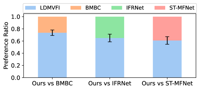
Following previous works (Liu et al. 2017; Niklaus and Liu 2018; Kalluri et al. 2023), the 2AFC approach is adopted for the subjective experiment, where the participant is asked to choose the one with better perceived quality from a pair of videos. Specifically, in each test session, the participant was displayed 66 pairs of videos where one video in each pair is interpolated by LDMVFI and the other is interpolated by ST-MFNet, IFRNet or BMBC. The display order of the 66 pairs, and the order of test videos within each pair are both randomized. The user is unaware of the methods used for generating the videos. Each pair is presented twice to the participant, who is then asked to provide an answer to the question “which of the two videos is of higher quality?”. Twenty participants were hired in total. See Appendix H for more details.

Results.

After collecting all the user data, for each of the 22 source sequences, the ratio of users that preferred LDMVFI is calculated. Figure 4 reports the average preference ratios for LDMVFI and the standard error over the sequences. It can be seen that in all comparisons, LDMVFI achieved higher preference ratios. T-test analysis (see Appendix H) on the sequence-wise preference ratios shows that the advantage of LDMVFI over the other three tested methods is statistically significant at 95% confidence level. These results further confirm the superior perceptual performance of LDMVFI.

Visual Examples.

Figure 3 shows example frames interpolated by LDMVFI and the competing methods, clearing demonstrating that the LDMVFI results have the best visual quality. See more visual examples in Appendix L.

5.3 Ablation Study

In this section we experimentally validate and study different components and hyper-parameters in LDMVFI. The ablation study results are summarized in Table 3, which shows evaluation results of 6 variants of the proposed model on three test sets. See Appendix G for full ablation study results, where more aspects of the model are analyzed, including discussions on the variability of LDMVFI results.

Effectiveness of VQ-FIGAN.

To validate the effectiveness of the proposed VQ-FIGAN design, we tested two variants of the model: V1 and V2. V2 outputs the frame $\hat{I}^{n}$ directly instead of predicting the deformable kernels, i.e. the convolutional heads after the last Conv3x3 layer are removed (see Figure 2). For V1, a further change is made by removing the feature-aided reconstruction process that involves $\phi^{0},\phi^{1}$ and replacing MaxCABlocks in the decoder with ResNetBlocks. As such, there is no information from the neighbor frames during decoding. Note that V1 is similar to the original VQGAN (Esser, Rombach, and Ommer 2021). Table 3 shows that without the deformable convolution-based synthesis, the performance of V2 sees an evident decrease. Furthermore, V1 shows a more severe drop in performance indicating the effectiveness of using features of neighbor frames during reconstruction.

Downsampling Factor $f$.

Here we study how the dimension of the latent space affects the VFI performance. Specifically, to obtain V4 ($f=16$), we remove one ResNetBlock+Conv3x3 layer and one ResNetBlock+MaxCABlock+Upsample+Conv3x3 layer from the encoder and decoder of VQ-FIGAN respectively (see Figure 2). We repeat this process once to obtain V3 ($f=8$). To create V5 ($f=64$) we add these layers instead of removing them. Table 3 shows that as $f$ increases from $8$ to $32$, there is generally an increasing trend in model performance (except that V4 outperformed LDMVFI on Middlebury). Such improvement is more obvious on DAVIS which mainly contains challenging large motion content. However, looking at $f=64$, the general performance deteriorates (in terms of LPIPS and FloLPIPS). The reason for this can be that to a reasonable extent, increasing $f$ allows the VQ-FIGAN decoder to make use of more information from the neighboring frames which can benefit frame interpolation, while preserving sufficient information for conditional generation in the latent space. However, if the downsampling is too aggressive, the information needed to perform reverse latent diffusion can be insufficient, resulting in degraded quality of latent generation. A similar trade-off between downsampling factor and model performance was also observed in (Rombach et al. 2022).

Effectiveness of Diffusion Process.

Here (V6) the denoising U-Net, hence the reverse diffusion process, is removed, and the decoder directly takes as input the concatenation of $z^{0}$ and $z^{1}$. Table 3 shows that without the diffusion process, the performance drops significantly, implying the effectiveness of the latent diffusion.

6 Conclusion

In this work we propose LDMVFI, the first approach that addresses video frame interpolation as a conditional generation problem using latent diffusion models. It contains two major components: an autoencoding model that provides access to a compact latent space, and a denoising U-Net that performs reverse diffusion on latent representations. To leverage latent diffusion models for VFI, we present several innovative designs including a VFI-specific autoencoding network, VQ-FIGAN, which employs efficient self-attention modules and deformable kernel-based frame synthesis techniques. LDMVFI was comprehensively evaluated on a wide range of test sets (including 4K content) using both quantitative metrics and subjective experiments. The results demonstrate its favorable perceptual performance over the state of the art.

Acknowledgements.

This work was supported in part by the China Scholarship Council, in part by the University of Bristol, and in part by the UK Research and Innovation (UKRI) MyWorld Strength in Places Program.

Appendix A Details of LDMVFI Loss Function (Diffusion Part)

In this section, we derive the training objective of the denoising U-Net in LDMVFI which is responsible for performing conditional generation. As mentioned in the main paper, diffusion models consist of a forward diffusion and a reverse denoising process. The forward diffusion process is defined by a Markov chain that gradually adds noise to a “clean” image $x_{0}$ using a pre-defined noise schedule $\{\beta_{t}\}_{t=1}^{T}$ in $T$ steps, with conditional probabilities

$$q(x_{t}|x_{t-1})=\mathcal{N}(x_{t};\sqrt{1-\beta_{t}}x_{t-1},\beta_{t}\mathbf{I}),$$ (7)

$$\Rightarrow\quad q(x_{1:T}|x_{0})=\prod_{t=1}^{T}q(x_{t}|x_{t-1}).$$ (8)

Let $\alpha_{t}=1-\beta_{t}$ and $\bar{\alpha}_{t}=\prod_{i=1}^{t}\alpha_{i}$, according to the conditional independence property of Markov chain, one can sample from the forward diffusion process at an arbitrary time step $t$ with

$$q(x_{t}|x_{0})=\mathcal{N}(x_{t};\sqrt{\bar{\alpha}_{t}}x_{0},(1-\bar{\alpha}_{t})\mathbf{I}).$$ (9)

In order to sample $x_{t}$ from this distribution in practice, we can use a reparameterization

$$x_{t}=\sqrt{\bar{\alpha}_{t}}x_{0}+\sqrt{1-\bar{\alpha}_{t}}\epsilon\quad\text{where}\quad\epsilon\sim\mathcal{N}(\mathbf{0},\mathbf{I}).$$ (10)

Here the noise schedule $\{\beta_{t}\}_{t=1}^{T}$ is designed such that $\bar{\alpha}_{T}\approx 0$ and $q(x_{T}|x_{0})\approx\mathcal{N}(x_{T};\mathbf{0},\mathbf{I})$. That is, as the forward diffusion process comes to an end, the last state of the image becomes close to a pure Gaussian noise.

Given the forward diffusion process, one could generate new samples by starting from pure Gaussian noise and sampling from the reverse conditionals $q(x_{t-1}|x_{t})$. However, $q(x_{t-1}|x_{t})$ is intractable, so one can use a $\theta$-parameterized Gaussian distribution

$$p_{\theta}(x_{t-1}|x_{t})=\mathcal{N}(x_{t-1};\mu_{\theta}(x_{t},t),\sigma_{t}^{2}\mathbf{I}),$$ (11)

$$\Rightarrow\quad p_{\theta}(x_{0:T})=p(x_{T})\prod_{t=1}^{T}p_{\theta}(x_{t-1}|x_{t}),$$ (12)

to approximate the reverse Markov chain (provided that $\beta_{t}$ is sufficiently small in each forward step (Sohl-Dickstein et al. 2015)). Here $\mu_{\theta}$ corresponds to a neural network, and $\sigma_{t}^{2}$ can be set to a value based on $\beta_{t}$ (Ho, Jain, and Abbeel 2020; Li et al. 2022; Rombach et al. 2022). One can then derive (Yang et al. 2022; Ho, Jain, and Abbeel 2020) the variational lower bound on the data log-likelihood:

$$\mathbb{E}_{q(x_{0})}[-\log p_{\theta}(x_{0})]\leq\mathbb{E}_{q(x_{0})q(x_{1:T}|x_{0})}\Big{[}-\log\frac{p_{\theta}(x_{0:T})}{q(x_{1:T}|x_{0})}\Big{]}=:L,$$ (13)

and training can be done by minimizing $L$. It can be shown (Sohl-Dickstein et al. 2015; Ho, Jain, and Abbeel 2020) that $L$ can be decomposed as

$$L=\mathbb{E}_{q}\Big{[}D_{\mathrm{KL}}\big{(}q(x_{T}|x_{0})||p_{\theta}(x_{T})\big{)}+\sum_{t=2}^{T}D_{\mathrm{KL}}\big{(}q(x_{t-1}|x_{t},x_{0})||p_{\theta}(x_{t-1}|x_{t})\big{)}-\log p_{\theta}(x_{0}|x_{1})\Big{]}.$$ (14)

The first term in (14) can be ignored because the prior $p_{\theta}(x_{T})$ can be set to a standard normal distribution, and the last term was handled by a separate decoder in (Ho, Jain, and Abbeel 2020), leaving the second term as the main focus for learning the reverse diffusion process. The $q(x_{t-1}|x_{t},x_{0})$ in the second term is tractable and it can be derived as

$$q(x_{t-1}|x_{t},x_{0})=\mathcal{N}(x_{t-1};\tilde{\mu}_{t}(x_{t},x_{0}),\tilde{\beta}_{t}\mathbf{I}),$$ (15)

where

$$\tilde{\mu}_{t}(x_{t},x_{0})=\frac{\sqrt{\bar{\alpha}_{t-1}}\beta_{t}}{1-\bar{\alpha}_{t}}x_{0}+\frac{\sqrt{\alpha_{t}}(1-\bar{\alpha}_{t-1})}{1-\bar{\alpha}_{t}}x_{t},$$ (16)

$$\tilde{\beta}_{t}=\frac{1-\bar{\alpha}_{t-1}}{1-\bar{\alpha}_{t}}\beta_{t}.$$ (17)

Since both $q(x_{t-1}|x_{t},x_{0})$ and $p_{\theta}(x_{t-1}|x_{t})$ are Gaussian distributions, the KL-divergence in the second term in (14) takes the form

$$L_{t-1}=:D_{\mathrm{KL}}\big{(}q(x_{t-1}|x_{t},x_{0})||p_{\theta}(x_{t-1}|x_{t})\big{)}=\mathbb{E}_{q}\Big{[}\frac{1}{2\sigma_{t}^{2}}\left\lVert\tilde{\mu}(x_{t},x_{0})-\mu_{\theta}(x_{t},t)\right\rVert^{2}\Big{]}.$$ (18)

In (Ho, Jain, and Abbeel 2020), it is noted that plugging (10) into $\tilde{\mu}(x_{t},x_{0})$, the latter can be written as

$$\tilde{\mu}(x_{t},x_{0})=\frac{1}{\sqrt{\alpha_{t}}}\big{(}x_{t}-\frac{1-\alpha_{t}}{\sqrt{1-\bar{\alpha}_{t}}}\epsilon\big{)}.$$ (19)

Therefore, it is proposed that instead of predicting $\mu_{\theta}(x_{t},t)$ directly, we can predict the noise $\epsilon_{\theta}(x_{t},t)$ then infer $\mu_{\theta}(x_{t},t)$ with

$$\mu_{\theta}(x_{t},t)=\frac{1}{\sqrt{\alpha_{t}}}\big{(}x_{t}-\frac{1-\alpha_{t}}{\sqrt{1-\bar{\alpha}_{t}}}\epsilon_{\theta}(x_{t},t)\big{)}.$$ (20)

Plugging in (19) and (20) into (18), the loss then reads

$$L_{t-1} =\mathbb{E}_{x_{0}\sim q(x_{0}),\epsilon\sim\mathcal{N}(\mathbf{0},\mathbf{I})}\Big{[}\frac{\beta_{t}^{2}}{2\sigma_{t}^{2}\alpha_{t}(1-\bar{\alpha}_{t})}\left\lVert\epsilon-\epsilon_{\theta}(x_{t},t)\right\rVert^{2}\Big{]}+C$$ (21)

$$=\mathbb{E}_{x_{0}\sim q(x_{0}),\epsilon\sim\mathcal{N}(\mathbf{0},\mathbf{I})}\Big{[}\frac{\beta_{t}^{2}}{2\sigma_{t}^{2}\alpha_{t}(1-\bar{\alpha}_{t})}\left\lVert\epsilon-\epsilon_{\theta}(\sqrt{\bar{\alpha}_{t}}x_{0}+\sqrt{1-\bar{\alpha}_{t}}\epsilon,t)\right\rVert^{2}\Big{]}+C,$$ (22)

where $C$ absorbs terms independent of $\theta$. It was observed in (Ho, Jain, and Abbeel 2020) that setting the multiplicative term before the norm in (22) to 1 provides improved performance, i.e.

$$L_{\mathrm{DM}}=\mathbb{E}_{x_{0},\epsilon\sim\mathcal{N}(\mathbf{0},\mathbf{I}),t\sim\mathcal{U}(1,T)}\big{[}\left\lVert\epsilon-\epsilon_{\theta}(x_{t},t)\right\rVert^{2}\big{]},$$ (23)

which corresponds to a re-weighted version of the variational lower bound. Latent diffusion models (LDMs) adopt the similar overall framework derived above, but performs the diffusion processes in a lower-dimensional latent space provided by an autoencoding model that contains an encoder $E:x\mapsto z$ and a decoder $D:z\mapsto x$. Accordingly, the noise predictor $\epsilon_{\theta}$ in LDMs are trained to optimize

$$L_{\mathrm{LDM}}=\mathbb{E}_{E(x_{0}),\epsilon\sim\mathcal{N}(\mathbf{0},\mathbf{I}),t\sim\mathcal{U}(1,T)}\big{[}\left\lVert\epsilon-\epsilon_{\theta}(z_{t},t)\right\rVert^{2}\big{]}.$$ (24)

In LDMVFI, the noise prediction also conditions on the latent encodings $z^{0}=E(I^{0}),z^{1}=E(I^{1})$ of the two input frames $I^{0},I^{1}$, and the loss we use becomes

$$\mathcal{L} =\mathbb{E}_{z^{n},z^{0},z^{1},\epsilon\sim\mathcal{N}(\mathbf{0},\mathbf{I}),t\sim\mathcal{U}(1,T)}\big{[}\left\lVert\epsilon-\epsilon_{\theta}(z^{n}_{t},t,z^{0},z^{1})\right\rVert^{2}\big{]}$$ (25)

$$=\mathbb{E}_{z^{n},z^{0},z^{1},\epsilon\sim\mathcal{N}(\mathbf{0},\mathbf{I}),t\sim\mathcal{U}(1,T)}\big{[}\left\lVert\epsilon-\epsilon_{\theta}(\sqrt{\bar{\alpha}_{t}}z^{n}_{0}+\sqrt{1-\bar{\alpha}_{t}}\epsilon,t,z^{0},z^{1})\right\rVert^{2}\big{]}.$$ (26)

Appendix B Details of LDMVFI Training and Inference

The full training and inference algorithms are summarized in Algorithm 1 and 2. Here the symbols and equations refer to those derived in Section A above.

Appendix C Details of DDIM Sampling Process

As stated in the main paper, in order to sample from LDMVFI and other diffusion models, we use the DDIM (Song, Meng, and Ermon 2021) sampler, which has been shown to achieve sampling quality on par with the full original sampling method (Algorithm 2), but with fewer steps. We refer the reader to the original paper for details on the derivation and design of DDIM, and present the DDIM sampling procedure for LDMVFI in Algorithm 3.

Algorithm 1 Training

1:  Input: dataset $\mathcal{D}=\{I^{0}_{s},I^{n}_{s},I^{1}_{s}\}_{s=1}^{S}$ of consecutive frame triplets, maximum diffusion step $T$, noise schedule $\{\beta_{t}\}_{t=1}^{T}$

2:  Load: pre-trained VQ-FIGAN encoder $E$

3:  Initialize: denoising U-Net $\epsilon_{\theta}$

4:  Compute $\{\bar{\alpha}_{t}\}_{t=1}^{T}$ from $\{\beta_{t}\}_{t=1}^{T}$

5:  repeat

6:     Sample $(I^{0},I^{n},I^{1})\sim\mathcal{D}$

7:     Encode $z^{0}=E(I^{0}),z^{n}=E(I^{n}),z^{1}=E(I^{1})$

8:     Sample $t\sim\mathcal{U}(1,T)$

9:     Sample $\epsilon\sim\mathcal{N}(\mathbf{0},\mathbf{I})$

10:     $z^{n}_{t}=\sqrt{\bar{\alpha}_{t}}z^{n}+\sqrt{1-\bar{\alpha}_{t}}\epsilon$

11:     Take a gradient descent step on       $\nabla_{\theta}\left\lVert\epsilon-\epsilon_{\theta}(z^{n}_{t},t,z^{0},z^{1})\right\rVert^{2}$

12:  until converged

Algorithm 2 Inference

1:  Input: original frames $I^{0},I^{1}$, noise schedule $\{\beta_{t}\}_{t=1}^{T}$, maximum diffusion step $T$

2:  Load: pre-trained denoising U-Net $\epsilon_{\theta}$, VQ-FIGAN encoder $E$ and decoder $D$

3:  Compute $\{\bar{\alpha}_{t}\}_{t=1}^{T}$ from $\{\beta_{t}\}_{t=1}^{T}$

4:  Sample $z^{n}_{T}\sim\mathcal{N}(\mathbf{0},\mathbf{I})$

5:  Encode $z^{0}=E(I^{0}),z^{1}=E(I^{1})$ and store features $\phi^{0},\phi^{1}$ extracted by $E$

6:  for $t=T,\dots,1$ do

7:     Predict noise $\hat{\epsilon}=\epsilon_{\theta}(z^{n}_{t},t,z^{0},z^{1})$

8:     $\mu_{\theta}=\frac{1}{\sqrt{\alpha_{t}}}\big{(}z^{n}_{t}-\frac{1-\alpha_{t}}{\sqrt{1-\bar{\alpha}_{t}}}\hat{\epsilon}\big{)}$

9:     $\sigma^{2}_{t}=\tilde{\beta}_{t}$

10:     Sample $\zeta\sim\mathcal{N}(\mathbf{0},\mathbf{I})$

11:     $z^{n}_{t-1}=\mu_{\theta}+\sigma_{t}\zeta$

12:  end for

13:  return $\hat{I}^{n}=D(z^{n}_{0},\phi^{0},\phi^{1})$ as the interpolated frame

Algorithm 3 DDIM Sampling for LDMVFI

1:  Input: original frames $I^{0},I^{1}$, noise schedule $\{\beta_{t}\}_{t=1}^{T}$, maximum DDIM step $\mathcal{T}$

2:  Load: pre-trained denoising U-Net $\epsilon_{\theta}$, VQ-FIGAN encoder $E$ and decoder $D$

3:  Compute $\{\bar{\alpha}_{t}\}_{t=1}^{T}$ from $\{\beta_{t}\}_{t=1}^{T}$

4:  Sample $z^{n}_{\mathcal{T}}\sim\mathcal{N}(\mathbf{0},\mathbf{I})$

5:  Encode $z^{0}=E(I^{0}),z^{1}=E(I^{1})$ and store features $\phi^{0},\phi^{1}$ extracted by $E$

6:  for $t=\mathcal{T},\dots,1$ do

7:     Predict noise $\hat{\epsilon}=\epsilon_{\theta}(z^{n}_{t},t,z^{0},z^{1})$

8:     $\hat{z}^{n}_{0}=\frac{1}{\sqrt{\bar{\alpha}_{t}}}(z^{n}_{t}-\sqrt{1-\bar{\alpha}_{t}}\hat{\epsilon})$

9:     $z^{n}_{t-1}=\sqrt{\bar{\alpha}_{t-1}}\hat{z}^{n}_{0}+\sqrt{1-\bar{\alpha}_{t-1}}\hat{\epsilon}$

10:  end for

11:  return $\hat{I}^{n}=D(z^{n}_{0},\phi^{0},\phi^{1})$ as the interpolated frame

Appendix D Denoising U-Net Architecture

The high-level architecture of the denoising U-Net used in LDMVFI is shown in Figure 5. As stated in the main paper, one modification from its original version in (Rombach et al. 2022) is to replace all vanilla self-attention layers with the MaxViT blocks (Tu et al. 2022). Figure 5 demonstrates how the hyper-parameter $c$ (the base channel size) affects the overall model size. We refer the reader to the original papers (Ho, Jain, and Abbeel 2020; Dhariwal and Nichol 2021; Rombach et al. 2022) and to our code for full details of the U-Net.

Figure 5: The architecture of the denoising U-Net. The hyper-parameter $c$ is a base channel size, which is set to 256 in LDMVFI. In each block, the $(\cdot\rightarrow\cdot)$ indicates the input and output channels of the block.

Appendix E Full Quantitative Evaluation Results

The full evaluation results of LDMVFI and the compared VFI methods on all test sets (Middlebury (Baker et al. 2011), UCF-101 (Soomro, Zamir, and Shah 2012), DAVIS (Perazzi et al. 2016), VFITex and SNU-FILM (Choi et al. 2020)) in terms of all metrics (PSNR, SSIM (Wang et al. 2004), LPIPS (Zhang et al. 2018), FloLPIPS (Danier, Zhang, and Bull 2022b) and FID (Heusel et al. 2017)) are summarized in Table 4.

	Middlebury					UCF-101
	PSNR$\uparrow$	SSIM$\uparrow$	LPIPS$\downarrow$	FloLPIPS$\downarrow$	FID$\downarrow$	PSNR$\uparrow$	SSIM$\uparrow$	LPIPS$\downarrow$	FloLPIPS$\downarrow$	FID$\downarrow$
BMBC	36.368	0.982	0.023	0.037	12.974	32.576	0.968	0.034	0.045	33.171
AdaCoF	35.256	0.975	0.031	0.052	15.633	32.488	0.968	0.034	0.046	32.783
CDFI	36.205	0.981	0.022	0.043	12.224	32.541	0.968	0.036	0.049	33.742
XVFI	34.724	0.975	0.036	0.070	16.959	32.224	0.966	0.038	0.050	33.868
ABME	37.639	0.986	0.027	0.040	11.393	32.055	0.967	0.058	0.069	37.066
IFRNet	36.368	0.983	0.020	0.039	12.256	32.716	0.969	0.032	0.044	28.803
VFIformer	35.566	0.977	0.031	0.065	15.634	32.745	0.968	0.039	0.051	34.112
ST-MFNet	N/A	N/A	N/A	N/A	N/A	33.383	0.970	0.036	0.049	34.475
FLAVR	N/A	N/A	N/A	N/A	N/A	33.224	0.969	0.035	0.046	31.449
MCVD	20.539	0.820	0.123	0.138	41.053	18.775	0.710	0.155	0.169	102.054
LDMVFI	34.033	0.971	0.019	0.044	16.167	32.186	0.963	0.026	0.035	26.301

	DAVIS					VFITex
	PSNR$\uparrow$	SSIM$\uparrow$	LPIPS$\downarrow$	FloLPIPS$\downarrow$	FID$\downarrow$	PSNR$\uparrow$	SSIM$\uparrow$	LPIPS$\downarrow$	FloLPIPS$\downarrow$	FID$\downarrow$
BMBC	26.835	0.869	0.125	0.185	15.354	27.337	0.904	0.220	0.282	50.393
AdaCoF	26.234	0.850	0.148	0.198	17.194	27.394	0.904	0.204	0.273	42.255
CDFI	26.471	0.857	0.157	0.211	18.098	27.577	0.906	0.218	0.286	43.498
XVFI	26.475	0.861	0.129	0.185	16.163	27.625	0.907	0.188	0.255	42.055
ABME	26.861	0.865	0.151	0.209	16.931	26.765	0.901	0.254	0.341	53.317
IFRNet	27.313	0.877	0.114	0.170	14.227	27.770	0.909	0.200	0.273	42.266
VFIformer	26.241	0.850	0.191	0.242	21.702	OOM	OOM	OOM	OOM	OOM
ST-MFNet	28.287	0.895	0.125	0.181	15.626	29.175	0.929	0.216	0.276	41.971
FLAVR	27.104	0.862	0.209	0.248	22.663	28.471	0.915	0.234	0.295	56.690
MCVD	18.946	0.705	0.247	0.293	28.002	OOM	OOM	OOM	OOM	OOM
LDMVFI	25.541	0.833	0.107	0.153	12.554	27.001	0.891	0.150	0.207	32.316

	SNU-FILM-Easy					SNU-FILM-Medium
	PSNR$\uparrow$	SSIM$\uparrow$	LPIPS$\downarrow$	FloLPIPS$\downarrow$	FID$\downarrow$	PSNR$\uparrow$	SSIM$\uparrow$	LPIPS$\downarrow$	FloLPIPS$\downarrow$	FID$\downarrow$
BMBC	39.809	0.990	0.020	0.031	6.162	35.437	0.978	0.034	0.059	12.272
AdaCoF	39.632	0.990	0.021	0.033	6.587	34.919	0.975	0.039	0.066	14.173
CDFI	39.881	0.990	0.019	0.031	6.133	35.224	0.977	0.036	0.066	12.906
XVFI	38.903	0.989	0.022	0.037	7.401	34.552	0.975	0.039	0.072	16.000
ABME	39.697	0.990	0.022	0.034	6.363	35.280	0.977	0.042	0.076	15.159
IFRNet	39.881	0.990	0.019	0.030	5.939	35.668	0.979	0.033	0.058	12.084
ST-MFNet	40.775	0.992	0.019	0.031	5.973	37.111	0.984	0.036	0.061	11.716
FLAVR	40.161	0.990	0.022	0.034	6.320	36.020	0.979	0.049	0.077	15.006
MCVD	22.201	0.828	0.199	0.230	32.246	21.488	0.812	0.213	0.243	37.474
LDMVFI	38.674	0.987	0.014	0.024	5.752	33.996	0.970	0.028	0.053	12.485

	SNU-FILM-Hard					SNU-FILM-Extreme
	PSNR$\uparrow$	SSIM$\uparrow$	LPIPS$\downarrow$	FloLPIPS$\downarrow$	FID$\downarrow$	PSNR$\uparrow$	SSIM$\uparrow$	LPIPS$\downarrow$	FloLPIPS$\downarrow$	FID$\downarrow$
BMBC	29.942	0.933	0.068	0.118	25.773	24.715	0.856	0.145	0.237	49.519
AdaCoF	29.477	0.925	0.080	0.131	27.982	24.650	0.851	0.152	0.234	52.848
CDFI	29.660	0.929	0.081	0.141	29.087	24.645	0.854	0.163	0.255	53.916
XVFI	29.364	0.928	0.075	0.138	29.483	24.545	0.853	0.142	0.233	54.449
ABME	29.643	0.929	0.092	0.168	34.236	24.541	0.853	0.182	0.300	63.561
IFRNet	30.143	0.935	0.065	0.122	25.436	24.954	0.859	0.136	0.229	50.047
ST-MFNet	31.698	0.951	0.073	0.123	25.512	25.810	0.874	0.148	0.238	53.563
FLAVR	30.577	0.938	0.112	0.169	34.746	25.206	0.861	0.217	0.303	72.673
MCVD	20.314	0.766	0.250	0.292	51.529	18.464	0.694	0.320	0.385	83.156
LDMVFI	28.547	0.917	0.060	0.114	26.520	23.934	0.837	0.123	0.204	47.042

Table 4: Quantitative comparison results on Middlebury, UCF-101, DAVIS, VFITex, and four subsets of SNU-FILM. Note ST-MFNet and FLAVR require four input frames so cannot be evaluated on Middlebury that contains frame triplets. VFIformer evaluation on SNU-FILM causes the GPU to go out of memory (OOM).

	Middlebury					UCF-101
	PSNR$\uparrow$	SSIM$\uparrow$	LPIPS$\downarrow$	FloLPIPS$\downarrow$	FID$\downarrow$	PSNR$\uparrow$	SSIM$\uparrow$	LPIPS$\downarrow$	FloLPIPS$\downarrow$	FID$\downarrow$
BMBC	36.787	0.984	0.021	0.036	14.968	32.729	0.969	0.032	0.042	33.024
AdaCoF	35.715	0.978	0.029	0.052	15.634	32.610	0.968	0.033	0.044	31.787
CDFI	37.140	0.985	0.011	0.022	6.645	32.653	0.968	0.024	0.033	23.856
XVFI	36.103	0.981	0.022	0.048	13.609	32.650	0.968	0.033	0.044	28.753
ABME	37.639	0.986	0.027	0.040	11.393	32.055	0.967	0.058	0.069	37.066
IFRNet	37.356	0.986	0.015	0.030	10.029	32.843	0.969	0.031	0.042	27.925
VFIformer	38.404	0.987	0.015	0.024	9.439	32.959	0.970	0.034	0.047	32.734
LDMVFI	34.230	0.974	0.019	0.041	35.745	32.160	0.964	0.026	0.034	25.792

	DAVIS					VFITex
	PSNR$\uparrow$	SSIM$\uparrow$	LPIPS$\downarrow$	FloLPIPS$\downarrow$	FID$\downarrow$	PSNR$\uparrow$	SSIM$\uparrow$	LPIPS$\downarrow$	FloLPIPS$\downarrow$	FID$\downarrow$
BMBC	26.293	0.855	0.131	0.187	15.136	26.784	0.899	0.201	0.266	35.493
AdaCoF	25.992	0.840	0.146	0.197	16.102	27.003	0.894	0.194	0.264	31.371
CDFI	26.403	0.849	0.106	0.149	11.418	27.278	0.899	0.160	0.228	32.765
XVFI	26.222	0.850	0.141	0.200	14.856	23.352	0.871	0.247	0.316	45.873
ABME	26.861	0.865	0.151	0.209	16.931	26.765	0.901	0.254	0.341	53.317
IFRNet	27.080	0.868	0.106	0.156	12.422	27.790	0.910	0.180	0.249	36.431
VFIformer	27.204	0.869	0.127	0.184	14.407	OOM	OOM	OOM	OOM	OOM
LDMVFI	25.073	0.819	0.125	0.172	14.093	26.355	0.887	0.161	0.224	36.831

	SNU-FILM-Easy					SNU-FILM-Medium
	PSNR$\uparrow$	SSIM$\uparrow$	LPIPS$\downarrow$	FloLPIPS$\downarrow$	FID$\downarrow$	PSNR$\uparrow$	SSIM$\uparrow$	LPIPS$\downarrow$	FloLPIPS$\downarrow$	FID$\downarrow$
BMBC	39.897	0.990	0.018	0.029	5.661	35.310	0.977	0.034	0.060	12.122
AdaCoF	39.801	0.990	0.019	0.030	6.007	35.050	0.975	0.036	0.065	13.287
CDFI	40.116	0.990	0.013	0.021	4.641	35.501	0.978	0.024	0.045	10.035
XVFI	39.554	0.989	0.020	0.033	6.629	35.062	0.976	0.037	0.069	14.021
ABME	39.697	0.990	0.022	0.034	6.363	35.280	0.977	0.042	0.076	15.159
IFRNet	40.107	0.991	0.017	0.027	5.429	35.851	0.979	0.029	0.050	10.745
VFIformer	40.204	0.991	0.018	0.028	5.682	36.028	0.980	0.033	0.056	11.188
LDMVFI	38.890	0.988	0.013	0.023	5.430	33.975	0.971	0.027	0.056	12.315

	SNU-FILM-Hard					SNU-FILM-Extreme
	PSNR$\uparrow$	SSIM$\uparrow$	LPIPS$\downarrow$	FloLPIPS$\downarrow$	FID$\downarrow$	PSNR$\uparrow$	SSIM$\uparrow$	LPIPS$\downarrow$	FloLPIPS$\downarrow$	FID$\downarrow$
BMBC	29.328	0.927	0.075	0.133	26.373	23.924	0.843	0.152	0.246	51.292
AdaCoF	29.463	0.924	0.075	0.127	26.707	24.307	0.844	0.148	0.233	50.278
CDFI	29.745	0.928	0.056	0.099	20.829	24.542	0.847	0.121	0.198	43.418
XVFI	29.510	0.927	0.075	0.132	28.167	24.435	0.848	0.143	0.231	50.851
ABME	29.643	0.929	0.092	0.168	34.236	24.541	0.853	0.182	0.300	63.561
IFRNet	30.150	0.934	0.058	0.109	22.512	24.795	0.856	0.128	0.216	45.458
VFIformer	30.256	0.935	0.069	0.124	24.268	24.921	0.858	0.146	0.235	47.378
LDMVFI	28.144	0.911	0.068	0.124	28.726	23.349	0.827	0.139	0.226	51.022

Table 5: Quantitative comparison results on Middlebury, UCF-101, DAVIS, VFITex, and four subsets of SNU-FILM for models trained with Vimeo90k-triplet only.

Appendix F Additional Quantitative Evaluation with Vimeo90k-triplet Training

In the main paper and Section E the evaluation results for models trained using the combination of Vimeo90k-septuplet and BVI-DVC are presented. Here we additionally include evaluation results for the models trained only with the Vimeo90k-triplet dataset. Note that here we only include models whose pre-trained versions (on the Vimeo90k-triplet dataset) are publicly available. These results are summerized in Table 5. Comparing Table 5 and Table 4, it is noticed that for some methods, the re-trained version on Vimeo90k+BVI-DVC show some extent of PSNR performance drop on the Middlebury and UCF-101 testsets. This can be due to the fact that Middlebury and UCF-101 show higher distribution overlap with the pre-training dataset Vimeo90k-triplet, while re-training on BVI-DVC+Vimeo90k shifts the training data distribution. Such shift towards content with larger and more complex motion (i.e. content from BVI-DVC) indeed shows benefits for the more challenging test sets such as DAVIS and VFITex, which are reflected in the increase in overall PSNR performance after re-training.

	$f$	$c$	AE Model	Cond. Mode	Middlebury			UCF-101			DAVIS
					LPIPS$\downarrow$	FloLPIPS$\downarrow$	FID$\downarrow$	LPIPS$\downarrow$	FloLPIPS$\downarrow$	FID$\downarrow$	LPIPS$\downarrow$	FloLPIPS$\downarrow$	FID$\downarrow$
V1	32	256	frame	concat	0.077	0.085	40.399	0.063	0.067	60.742	0.168	0.200	21.812
V2	32	256	MaxCA+frame	concat	0.028	0.045	19.485	0.032	0.041	29.578	0.135	0.176	19.980
V3	8	256	MaxCA+kernel	concat	0.018	0.046	19.552	0.028	0.036	27.278	0.125	0.168	15.535
V4	16	256	MaxCA+kernel	concat	0.017	0.037	12.539	0.026	0.035	26.805	0.107	0.154	12.720
V5	64	256	MaxCA+kernel	concat	0.022	0.044	15.041	0.026	0.036	26.055	0.114	0.157	12.330
V6	32	256	MaxCA+kernel	N/A	0.100	0.108	38.538	0.042	0.053	32.189	0.193	0.214	8.639
V7	32	64	MaxCA+kernel	concat	0.019	0.044	16.101	0.026	0.035	26.376	0.107	0.153	12.627
V8	32	128	MaxCA+kernel	concat	0.019	0.044	16.026	0.026	0.035	26.340	0.107	0.153	12.611
V9	32	256	MaxCA+kernel	MaxCA	0.019	0.044	16.005	0.026	0.035	26.334	0.106	0.153	12.571
Ours	32	256	MaxCA+kernel	concat	0.019	0.044	16.167	0.026	0.035	26.301	0.107	0.153	12.554

Table 6: Ablation experiment results, showing performance of variants of the proposed LDMVFI.

	SNU-FILM-Easy			SNU-FILM-Medium			SNU-FILM-Hard			SNU-FILM-Extreme
	LPIPS$\downarrow$	FloLPIPS$\downarrow$	FID$\downarrow$	LPIPS$\downarrow$	FloLPIPS$\downarrow$	FID$\downarrow$	LPIPS$\downarrow$	FloLPIPS$\downarrow$	FID$\downarrow$	LPIPS$\downarrow$	FloLPIPS$\downarrow$	FID$\downarrow$
V1	0.054	0.056	14.010	0.068	0.082	20.572	0.104	0.142	35.429	0.172	0.243	72.617
V2	0.020	0.028	7.779	0.035	0.058	15.138	0.076	0.126	32.653	0.150	0.233	69.730
V3	0.016	0.026	6.374	0.030	0.052	11.701	0.068	0.119	27.183	0.144	0.227	55.596
V4	0.014	0.024	5.982	0.027	0.052	11.987	0.059	0.112	25.088	0.122	0.204	47.623
V5	0.016	0.027	6.191	0.031	0.058	13.060	0.064	0.116	26.439	0.129	0.211	48.336
V6	0.083	0.086	20.134	0.103	0.111	24.124	0.141	0.160	29.157	0.201	0.237	35.021
V7	0.014	0.024	5.758	0.028	0.053	12.483	0.060	0.114	26.401	0.123	0.204	47.022
V8	0.014	0.024	5.754	0.028	0.053	12.483	0.060	0.114	26.380	0.123	0.204	46.882
V9	0.014	0.024	5.757	0.028	0.053	12.477	0.060	0.114	26.525	0.122	0.204	46.906
Ours	0.014	0.024	5.752	0.028	0.053	12.485	0.060	0.114	26.520	0.123	0.204	47.042

Table 7: Ablation experiment results on SNU-FILM. Full details of the variants (V1-8) can be found in the main paper.

Appendix G Full Ablation Study Results

In the main paper, due to space limitations, we presented selected ablation experiments on only three test sets. Here we provide the full ablation study, including additional experiments and evaluation on additional test sets.

Effect of Model Size.

We investigate how the model size of the denoising U-Net affects the performance. The denoising U-Net contains multiple layers of ResNet and MaxViT blocks, where the number of feature channels is a multiple of a base channel number $c$ (detailed in Figure 5). In the default LDMVFI, $c=256$. This corresponds to a total of 439.0M parameters. We experiment with $c=128,64$ (V8,V7), which reduce the model parameters to 126.8M and 48.7M respectively. It is observed from Table 6 and 7 that as $c$ is decreased, there is no significant change in performance. This may be because when $f=32$, the latent dimension is low enough ($8\times 8$ for training data) that the model capacity is still sufficient even when $c=64$. To verify this, we additionally tested $c=64,128,256$ for the case of $f=8$ (latent dimension is $32\times 32$ for training data). The results are shown in Table 8, where it is observed that as $c$ decreases, there is a clearer decreasing trend in overall model performance.

Conditioning Mechanism.

In LDMVFI, the mechanism for conditioning the denoising U-Net on the latents $z^{0},z^{1}$ is concatenation, i.e., we concatenate $z^{n}_{t},z^{0},z^{1}$ to form the U-Net input. In (Rombach et al. 2022), an alternative cross attention-based conditioning mechanism is introduced. Based on this, We create a variant of LDMVFI (V9) where the conditioning is done using MaxCA blocks at different layers of the U-Net. As shown in Table 6 and 7, V9 shows highly similar performance to LDMVFI. Given the limited improvement, we adopted the simpler concatenation-based conditioning for LDMVFI.

	$f$	$c$	AE Model	Cond. Mode	Middlebury			UCF-101			DAVIS
					LPIPS$\downarrow$	FloLPIPS$\downarrow$	FID$\downarrow$	LPIPS$\downarrow$	FloLPIPS$\downarrow$	FID$\downarrow$	LPIPS$\downarrow$	FloLPIPS$\downarrow$	FID$\downarrow$
V10	8	64	MaxCA+kernel	concat	0.020	0.040	13.800	0.029	0.037	28.831	0.133	0.179	17.937
V11	8	128	MaxCA+kernel	concat	0.019	0.035	13.528	0.028	0.036	26.917	0.131	0.175	17.746
V3	8	256	MaxCA+kernel	concat	0.018	0.046	19.552	0.028	0.036	27.278	0.125	0.168	15.535

	SNU-FILM-Easy			SNU-FILM-Medium			SNU-FILM-Hard			SNU-FILM-Extreme
	LPIPS$\downarrow$	FloLPIPS$\downarrow$	FID$\downarrow$	LPIPS$\downarrow$	FloLPIPS$\downarrow$	FID$\downarrow$	LPIPS$\downarrow$	FloLPIPS$\downarrow$	FID$\downarrow$	LPIPS$\downarrow$	FloLPIPS$\downarrow$	FID$\downarrow$
V10	0.016	0.026	6.255	0.032	0.060	13.312	0.076	0.132	30.786	0.157	0.243	62.075
V11	0.016	0.024	6.256	0.031	0.054	13.329	0.073	0.127	30.343	0.155	0.241	66.383
V3	0.016	0.026	6.374	0.030	0.052	11.701	0.068	0.119	27.183	0.144	0.227	55.596

Table 8: Ablation experiment results on $c$ when $f=8$.

(a)

(b)

(c)

(d)

(e)

(a) Overlaid Inputs

(b) Sample 1

(c) Sample 2

(d) Residual

(e) IFRNet

​​  ​​  ​​  ​​  ​​  ​​  ​​  ​​

Figure 6: Visual examples on variability of LDMVFI results. Residual is the difference between Sample 1 and Sample 2.

Variability of VFI results.

When non-deterministic samplers are used (e.g. DDPM (Ho, Jain, and Abbeel 2020)), diffusion models can produce varied results given the same input. We investigate such variability in VFI by sampling multiple times from LDMVFI using DDPM given the same frames. As illustrated in Figure 6, under relatively regular motions (e.g. that of rigid objects), there is little variation in the result, as shown by the residual image (the fourth column) between Sample 1 and Sample 2. This is desirable because in such cases there might only be one ground-truth frame and variation in the interpolation result can lead to temporal inconsistency. On the other hand, for dynamic textures (e.g. water) where the underlying motion can be quite irregular and random, LDMVFI does produce varied results. It is also noted that these results are much sharper than those of IFRNet, and this can be due to the fact that as a generative model, LDMVFI draws single samples from a distribution, while existing methods like IFRNet that are trained on L1 losses tend to learn an average of many possible results (i.e. the over-smoothing issue discussed in (Li et al. 2022)), which manifest as blur and causes flickering (see the supplementary video). This is further supported by the large performance gain of LDMVFI over existing methods on the VFITex dataset (Table 4).

Appendix H Details of Subjective Experiment

The user study and the use of human data have undergone an internal ethics review and have been approved by the Institutional Review Board.

The subjective experiment was conducted in a lab-based environment. The monitor used to display videos was a BENQ XL2720Z (59.8$\times$33.6cm screen size). The spatial resolution of the display was set to $1920\times 1080$ and the frame rate was set to $60$Hz. The viewing distance of the participants was 1 meter, approximately three times screen height (ITU-R BT 2002).

In the main paper, we state that t-tests are performed between the sequence-wise preference ratios of the proposed method and the three tested baselines. Here we report the $p$ values for the t-tests in Table 9.

Comparison	$p$ value
Ours vs BMBC	$3.8\times 10^{-9}$
Ours vs IFRNet	$1.6\times 10^{-3}$
Ours vs ST-MFNet	$1.7\times 10^{-2}$

Table 9: The results of t-test analysis on the user study results.

	PSNR$\uparrow$	SSIM$\uparrow$	LPIPS$\downarrow$	FloLPIPS$\downarrow$	FID$\downarrow$
ST-MFNet	21.709	0.780	0.226	0.297	28.939
IFRNet	22.745	0.813	0.186	0.270	23.122
LDMVFI	22.194	0.753	0.167	0.204	14.493

Table 10: Multi-frame ($\times$4) evaluation results on DAVIS.

Appendix I Multi-Frame ($\times$4) Interpolation

The $\times$4 up-sampling performance of LDMVFI is evaluated on the DAVIS (Perazzi et al. 2016) dataset. Specifically, in each sequence of DAVIS, every 2nd, 3rd and 4th frames are dropped and considered as the ground truth. The 3rd frame is firstly interpolated from the 1st and the 5th frame, then the 2nd frame is interpolated using the 1st and the 3rd frames (previously interpolated), and the 4th frame is interpolated in a similar way. For this experiment, we compared LDMVFI with the two most competitive approaches according to Table 4: IFRNet (Kong et al. 2022) and ST-MFNet (Danier, Zhang, and Bull 2022c). Table 10 shows that LDMVFI achieves the best scores in terms of the perceptual metrics (i.e. LPIPS, FloLPIPS and FID).

Appendix J Limitations and Societal Impact

Limitations.

Firstly, as discussed in the main paper, the proposed LDMVFI shows a much slower inference speed compared to the other state-of-the-art methods. This is a common drawback of diffusion models (Ho, Jain, and Abbeel 2020; Rombach et al. 2022) mainly due to the iterative reverse process during generation. Various techniques (Salimans and Ho 2022; Karras et al. 2022; Lu et al. 2022a) have been proposed to speed up the sampling process and these can also be applied to LDMVFI. Secondly, the number of model parameters in LDMVFI is also larger than other methods. The main component of LDMVFI that accounts for the large model size is the denoising U-Net, which was developed in previous work (Ho, Jain, and Abbeel 2020; Dhariwal and Nichol 2021; Rombach et al. 2022) and modified in here by replacing the self-attention layers with MaxViT blocks (Tu et al. 2022). To reduce the model size, techniques such as knowledge distillation (Hinton, Vinyals, and Dean 2015; Morris et al. 2023) and model compression (Buciluǎ, Caruana, and Niculescu-Mizil 2006) can be used. The exploration of these techniques, as well as the accelerated diffusion sampling methods in the context of VFI, remain for future work. Finally, we noticed that LDMVFI can generate unsatisfactory results under extremely large motion, which is a common challenge faced by many state-of-the-art VFI methods.

Potential Negative Societal Impact.

Firstly, in general, generative models for images and videos can be used to generate inappropriately manipulated content or in unethical ways (e.g. “deep fake” generation) (Denton 2021). Secondly, the two-stage training strategy, large model size and slow inference speed of LDMVFI mean that large-scale training and evaluation processes can consume significant amounts of energy, leading to increased carbon footprint (Lacoste et al. 2019). We refer the readers to (Denton 2021) and (Lacoste et al. 2019) for more detailed discussions on these matters.

Appendix K Attribution of Assets: Code and Data

In this section, we summarize the sources and licenses of all the datasets and code used in the work. The attribution of datasets and code are shown in Table 11 and 12. For MCVD (Voleti, Jolicoeur-Martineau, and Pal 2022), we used the smmnist_DDPM_big5.yml configuration, setting both the numbers of previous and future frames to 1, and the number of interpolated frames also to 1.

Dataset	Dataset URL	License / Terms of Use
Vimeo-90k (Xue et al. 2019)	http://toflow.csail.mit.edu	MIT license.
BVI-DVC (Ma, Zhang, and Bull 2021)	https://fan-aaron-zhang.github.io/BVI-DVC/ (original videos); https://github.com/danielism97/ST-MFNet (quintuplets)	All sequences are allowed for academic research.
UCF101 (Soomro, Zamir, and Shah 2012)	https://www.crcv.ucf.edu/research/data-sets/ucf101/	No explicit license terms, but compiled and made available for research use by the University of Central Florida.
DAVIS (Perazzi et al. 2016)	https://davischallenge.org	BSD license.
SNU-FILM (Choi et al. 2020)	https://myungsub.github.io/CAIN/	MIT license .
Middlebury (Baker et al. 2011)	https://vision.middlebury.edu/flow/data/	All sequences are available for research use.
VFITex (Danier, Zhang, and Bull 2022c)	https://github.com/danier97/ST-MFNet	All sequences are available for research use.
BVI-HFR (Mackin, Zhang, and Bull 2018)	https://fan-aaron-zhang.github.io/BVI-HFR/	Non-Commercial Government Licence for public sector information.

Table 11: License information for the datasets used in this work.

Method	Source code URL	License / Teams of Use
BMBC (Park et al. 2020)	https://github.com/JunHeum/BMBC	MIT license.
AdaCoF (Lee et al. 2020)	https://github.com/HyeongminLEE/AdaCoF-pytorch	MIT license.
CDFI (Ding et al. 2021)	https://github.com/tding1/CDFI	Available for research use.
XVFI (Sim, Oh, and Kim 2021)	https://github.com/JihyongOh/XVFI	Research and education only.
ABME (Park, Lee, and Kim 2021)	https://github.com/JunHeum/ABME	MIT license.
IFRNet (Kong et al. 2022)	https://github.com/ltkong218/IFRNet	MIT license.
VFIformer (Lu et al. 2022b)	https://github.com/dvlab-research/VFIformer	Available for research use.
ST-MFNet (Danier, Zhang, and Bull 2022c)	https://github.com/danielism97/ST-MFNet	MIT license.
FLAVR (Kalluri et al. 2023)	https://github.com/tarun005/FLAVR	Apache-2.0 license.
MCVD (Voleti, Jolicoeur-Martineau, and Pal 2022)	https://github.com/voletiv/mcvd-pytorch	MIT license.

Table 12: License information for the code assets used in this work.

Appendix L Additional Qualitative Examples

(a)

(b)

(c)

(d)

(e)

(f)

(g)

​​  ​​  ​​  ​​  ​​  ​​

(h)

(i)

(j)

(k)

(l)

(m)

(n)

​​  ​​  ​​  ​​  ​​  ​​

(o)

(p)

(q)

(r)

(s)

(t)

(u)

​​  ​​  ​​  ​​  ​​  ​​

(v)

(w)

(x)

(y)

(z)

(aa)

(ab)

​​  ​​  ​​  ​​  ​​  ​​

(ac)

(ad)

(ae)

(af)

(ag)

(ah)

(ai)

​​  ​​  ​​  ​​  ​​  ​​

(aj)

(ak)

(al)

(am)

(an)

(ao)

(ap)

​​  ​​  ​​  ​​  ​​  ​​

(a) Overlaid inputs

(b) GT

(c) BMBC

(d) VFIformer

(e) IFRNet

(f) ST-MFNet

(g) LDMVFI (ours)

Figure 7: Visual interpolation examples.

​​  ​​  ​​  ​​  ​​  ​​

(a)

(b)

(c)

(d)

(e)

(f)

(g)

​​  ​​  ​​  ​​  ​​  ​​

(h)

(i)

(j)

(k)

(l)

(m)

(n)

​​  ​​  ​​  ​​  ​​  ​​

(o)

(p)

(q)

(r)

(s)

(t)

(u)

​​  ​​  ​​  ​​  ​​  ​​

(a) Overlaid inputs

(b) GT

(c) BMBC

(d) VFIformer

(e) IFRNet

(f) ST-MFNet

(g) LDMVFI (ours)

Figure 8: Visual interpolation examples.

​​  ​​  ​​  ​​  ​​  ​​

References

- Baker et al. (2011) Baker, S.; Scharstein, D.; Lewis, J.; Roth, S.; Black, M. J.; and Szeliski, R. 2011. A database and evaluation methodology for optical flow. Int. J. of Comput. Vis., 92(1): 1–31.
- Bao et al. (2021) Bao, W.; Lai, W.-S.; Zhang, X.; Gao, Z.; and Yang, M.-H. 2021. MEMC-Net: Motion estimation and motion compensation driven neural network for video interpolation and enhancement. IEEE Trans. on Pattern Anal. Mach. Intell., 43(3): 933–948.
- Buciluǎ, Caruana, and Niculescu-Mizil (2006) Buciluǎ, C.; Caruana, R.; and Niculescu-Mizil, A. 2006. Model compression. In Proc. of the 12th ACM SIGKDD Int. Conf. on Knowledge Discovery and Data Mining, 535–541.
- Cheng and Chen (2020) Cheng, X.; and Chen, Z. 2020. Video frame interpolation via deformable separable convolution. In Proc. of the AAAI Conf. on Artificial Intell., 10607–10614.
- Cheng and Chen (2022) Cheng, X.; and Chen, Z. 2022. Multiple video frame interpolation via enhanced deformable separable convolution. IEEE Trans. on Pattern Anal. Mach. Intell., 44(10): 7029–7045.
- Choi et al. (2020) Choi, M.; Kim, H.; Han, B.; Xu, N.; and Lee, K. M. 2020. Channel attention is all you need for video frame interpolation. In Proc. of the AAAI Conf. on Artificial Intell., volume 34, 10663–10671.
- Dai et al. (2017) Dai, J.; Qi, H.; Xiong, Y.; Li, Y.; Zhang, G.; Hu, H.; and Wei, Y. 2017. Deformable convolutional networks. In Proc. of the IEEE Int. Conf. on Comput. Vis., 764–773.
- Danier, Zhang, and Bull (2022a) Danier, D.; Zhang, F.; and Bull, D. 2022a. Enhancing deformable convolution based video frame interpolation with coarse-to-fine 3D CNN. In IEEE Int. Conf. on Image Process., 1396–1400.
- Danier, Zhang, and Bull (2022b) Danier, D.; Zhang, F.; and Bull, D. 2022b. FloLPIPS: A Bespoke Video Quality Metric for Frame Interpolation. In IEEE Picture Coding Symposium, 283–287.
- Danier, Zhang, and Bull (2022c) Danier, D.; Zhang, F.; and Bull, D. 2022c. ST-MFNet: A spatio-temporal multi-flow network for frame interpolation. In Proc. of the IEEE Conf. on Comput. Vis. and Pattern Recog., 3521–3531.
- Danier, Zhang, and Bull (2022d) Danier, D.; Zhang, F.; and Bull, D. 2022d. A subjective quality study for video frame interpolation. In IEEE Int. Conf. on Image Process., 1361–1365.
- Denton (2021) Denton, E. 2021. Ethical considerations of generative ai. In AI for Content Creation Workshop, CVPR, volume 27.
- Dhariwal and Nichol (2021) Dhariwal, P.; and Nichol, A. 2021. Diffusion models beat gans on image synthesis. Adv. in Neural Inform. Process. Syst., 34: 8780–8794.
- Ding et al. (2021) Ding, T.; Liang, L.; Zhu, Z.; and Zharkov, I. 2021. CDFI: Compression-Driven Network Design for Frame Interpolation. In Proc. of the IEEE Conf. on Comput. Vis. and Pattern Recog., 8001–8011.
- Dosovitskiy et al. (2021) Dosovitskiy, A.; Beyer, L.; Kolesnikov, A.; Weissenborn, D.; Zhai, X.; Unterthiner, T.; Dehghani, M.; Minderer, M.; Heigold, G.; Gelly, S.; Uszkoreit, J.; and Houlsby, N. 2021. An Image is Worth 16x16 Words: Transformers for Image Recognition at Scale. In Int. Conf. on Learn. Represent.
- Esser, Rombach, and Ommer (2021) Esser, P.; Rombach, R.; and Ommer, B. 2021. Taming transformers for high-resolution image synthesis. In Proc. of the IEEE Conf. on Comput. Vis. and Pattern Recog., 12873–12883.
- Flynn et al. (2016) Flynn, J.; Neulander, I.; Philbin, J.; and Snavely, N. 2016. Deepstereo: Learning to predict new views from the world’s imagery. In Proc. of the IEEE Conf. on Comput. Vis. and Pattern Recog., 5515–5524.
- Goodfellow et al. (2020) Goodfellow, I.; Pouget-Abadie, J.; Mirza, M.; Xu, B.; Warde-Farley, D.; Ozair, S.; Courville, A.; and Bengio, Y. 2020. Generative adversarial networks. Communications of the ACM, 63(11): 139–144.
- Heusel et al. (2017) Heusel, M.; Ramsauer, H.; Unterthiner, T.; Nessler, B.; and Hochreiter, S. 2017. GANs trained by a two time-scale update rule converge to a local nash equilibrium. Adv. in Neural Inform. Process. Syst., 30.
- Hinton, Vinyals, and Dean (2015) Hinton, G.; Vinyals, O.; and Dean, J. 2015. Distilling the knowledge in a neural network. arXiv preprint arXiv:1503.02531.
- Ho, Jain, and Abbeel (2020) Ho, J.; Jain, A.; and Abbeel, P. 2020. Denoising diffusion probabilistic models. Adv. in Neural Inform. Process. Syst., 33: 6840–6851.
- Ho et al. (2022) Ho, J.; Saharia, C.; Chan, W.; Fleet, D. J.; Norouzi, M.; and Salimans, T. 2022. Cascaded Diffusion Models for High Fidelity Image Generation. J. of Machine Learning Research, 23(47): 1–33.
- Isola et al. (2017) Isola, P.; Zhu, J.-Y.; Zhou, T.; and Efros, A. A. 2017. Image-to-image translation with conditional adversarial networks. In Proc. of the IEEE Conf. on Comput. Vis. and Pattern Recog., 1125–1134.
- ITU-R BT (2002) ITU-R BT, R. 2002. 500-11, Methodology for the subjective assessment of the quality of television pictures,”. Int. Telecommunication Union, Tech. Rep.
- Jiang et al. (2018) Jiang, H.; Sun, D.; Jampani, V.; Yang, M.-H.; Learned-Miller, E.; and Kautz, J. 2018. Super slomo: High quality estimation of multiple intermediate frames for video interpolation. In Proc. of the IEEE Conf. on Comput. Vis. and Pattern Recog., 9000–9008.
- Kalluri et al. (2023) Kalluri, T.; Pathak, D.; Chandraker, M.; and Tran, D. 2023. FLAVR: Flow-agnostic video representations for fast frame interpolation. In Proc. of the IEEE Winter Conf. on Applications of Comput. Vis., 2071–2082.
- Kang et al. (2023) Kang, X.; Lin, X.; Zhang, K.; Hui, Z.; Xiang, W.; He, J.-Y.; Li, X.; Ren, P.; Xie, X.; Timofte, R.; et al. 2023. NTIRE 2023 video colorization challenge. In Proc. of the IEEE Conf. on Comput. Vis. and Pattern Recog., 1570–1581.
- Karargyris and Bourbakis (2010) Karargyris, A.; and Bourbakis, N. 2010. Three-dimensional reconstruction of the digestive wall in capsule endoscopy videos using elastic video interpolation. IEEE Trans. on Medical Imaging, 30(4): 957–971.
- Karras et al. (2022) Karras, T.; Aittala, M.; Aila, T.; and Laine, S. 2022. Elucidating the Design Space of Diffusion-Based Generative Models. In Oh, A. H.; Agarwal, A.; Belgrave, D.; and Cho, K., eds., Adv. in Neural Inform. Process. Syst., volume 35, 26565–26577.
- Kingma and Ba (2015) Kingma, D. P.; and Ba, J. 2015. Adam: A Method for Stochastic Optimization. In Int. Conf. on Learn. Represent.
- Kingma and Welling (2014) Kingma, D. P.; and Welling, M. 2014. Auto-Encoding Variational Bayes. In Int. Conf. on Learn. Represent.
- Kong et al. (2022) Kong, L.; Jiang, B.; Luo, D.; Chu, W.; Huang, X.; Tai, Y.; Wang, C.; and Yang, J. 2022. IFRNet: Intermediate feature refine network for efficient frame interpolation. In Proc. of the IEEE Conf. on Comput. Vis. and Pattern Recog., 1969–1978.
- Lacoste et al. (2019) Lacoste, A.; Luccioni, A.; Schmidt, V.; and Dandres, T. 2019. Quantifying the carbon emissions of machine learning. arXiv preprint arXiv:1910.09700.
- Lee et al. (2020) Lee, H.; Kim, T.; Chung, T.-y.; Pak, D.; Ban, Y.; and Lee, S. 2020. AdaCoF: Adaptive collaboration of flows for video frame interpolation. In Proc. of the IEEE Conf. on Comput. Vis. and Pattern Recog., 5316–5325.
- Li et al. (2022) Li, H.; Yang, Y.; Chang, M.; Chen, S.; Feng, H.; Xu, Z.; Li, Q.; and Chen, Y. 2022. Srdiff: Single image super-resolution with diffusion probabilistic models. Neurocomputing, 479: 47–59.
- Liu et al. (2017) Liu, Z.; Yeh, R. A.; Tang, X.; Liu, Y.; and Agarwala, A. 2017. Video frame synthesis using deep voxel flow. In Proc. of the IEEE Int. Conf. on Comput. Vis., 4463–4471.
- Loshchilov and Hutter (2019) Loshchilov, I.; and Hutter, F. 2019. Decoupled Weight Decay Regularization. In Int. Conf. on Learn. Represent.
- Lu et al. (2022a) Lu, C.; Zhou, Y.; Bao, F.; Chen, J.; Li, C.; and Zhu, J. 2022a. Dpm-solver: A fast ode solver for diffusion probabilistic model sampling in around 10 steps. Adv. in Neural Inform. Process. Syst., 35: 5775–5787.
- Lu et al. (2022b) Lu, L.; Wu, R.; Lin, H.; Lu, J.; and Jia, J. 2022b. Video frame interpolation with transformer. In Proc. of the IEEE Conf. on Comput. Vis. and Pattern Recog., 3532–3542.
- Ma, Zhang, and Bull (2021) Ma, D.; Zhang, F.; and Bull, D. 2021. BVI-DVC: A Training Database for Deep Video Compression. IEEE Trans. on Multimedia, 1–1.
- Mackin, Zhang, and Bull (2018) Mackin, A.; Zhang, F.; and Bull, D. R. 2018. A study of high frame rate video formats. IEEE Trans. on Multimedia, 21(6): 1499–1512.
- Men et al. (2020) Men, H.; Hosu, V.; Lin, H.; Bruhn, A.; and Saupe, D. 2020. Visual quality assessment for interpolated slow-motion videos based on a novel database. In IEEE Int. Conf. on Quality of Multimedia Experience, 1–6.
- Morris et al. (2023) Morris, C.; Danier, D.; Zhang, F.; Anantrasirichai, N.; and Bull, D. R. 2023. ST-MFNet Mini: Knowledge Distillation-Driven Frame Interpolation. arXiv preprint arXiv:2302.08455.
- Moss et al. (2015) Moss, F. M.; Wang, K.; Zhang, F.; Baddeley, R.; and Bull, D. R. 2015. On the optimal presentation duration for subjective video quality assessment. IEEE Trans. on Circuit Syst. Video Technol., 26(11): 1977–1987.
- Niklaus and Liu (2018) Niklaus, S.; and Liu, F. 2018. Context-aware synthesis for video frame interpolation. In Proc. of the IEEE Conf. on Comput. Vis. and Pattern Recog., 1701–1710.
- Niklaus and Liu (2020) Niklaus, S.; and Liu, F. 2020. Softmax splatting for video frame interpolation. In Proc. of the IEEE Conf. on Comput. Vis. and Pattern Recog., 5437–5446.
- Niklaus, Mai, and Liu (2017) Niklaus, S.; Mai, L.; and Liu, F. 2017. Video frame interpolation via adaptive convolution. In Proc. of the IEEE Conf. on Comput. Vis. and Pattern Recog., 670–679.
- Park et al. (2020) Park, J.; Ko, K.; Lee, C.; and Kim, C.-S. 2020. BMBC: Bilateral motion estimation with bilateral cost volume for video interpolation. In Comput. Vis.–ECCV 2020: 16th European Conference, Glasgow, UK, August 23–28, 2020, Proceedings, Part XIV 16, 109–125. Springer.
- Park, Lee, and Kim (2021) Park, J.; Lee, C.; and Kim, C.-S. 2021. Asymmetric Bilateral Motion Estimation for Video Frame Interpolation. In Proc. of IEEE Int. Conf. on Comput. Vis., 14539–14548.
- Perazzi et al. (2016) Perazzi, F.; Pont-Tuset, J.; McWilliams, B.; Van Gool, L.; Gross, M.; and Sorkine-Hornung, A. 2016. A benchmark dataset and evaluation methodology for video object segmentation. In Proc. of the IEEE Conf. on Comput. Vis. and Pattern Recog., 724–732.
- Rigamonti et al. (2013) Rigamonti, R.; Sironi, A.; Lepetit, V.; and Fua, P. 2013. Learning separable filters. In Proc. of the IEEE Conf. on Comput. Vis. and Pattern Recog., 2754–2761.
- Rombach et al. (2022) Rombach, R.; Blattmann, A.; Lorenz, D.; Esser, P.; and Ommer, B. 2022. High-resolution image synthesis with latent diffusion models. In Proc. of the IEEE Conf. on Comput. Vis. and Pattern Recog., 10684–10695.
- Saha et al. (2023) Saha, A.; Pentapati, S. K.; Shang, Z.; Pahwa, R.; Chen, B.; Gedik, H. E.; Mishra, S.; and Bovik, A. C. 2023. Perceptual Video Quality Assessment: The Journey Continues! Frontiers in Signal Processing, 3.
- Salimans and Ho (2022) Salimans, T.; and Ho, J. 2022. Progressive Distillation for Fast Sampling of Diffusion Models. In Int. Conf. on Learn. Represent.
- Sim, Oh, and Kim (2021) Sim, H.; Oh, J.; and Kim, M. 2021. XVFI: eXtreme Video Frame Interpolation. In Proc. of the IEEE Int. Conf. on Comput. Vis., 14489–14498.
- Simonyan and Zisserman (2015) Simonyan, K.; and Zisserman, A. 2015. Very Deep Convolutional Networks for Large-Scale Image Recognition. In Int. Conf. on Learn. Represent.
- Siyao et al. (2021) Siyao, L.; Zhao, S.; Yu, W.; Sun, W.; Metaxas, D.; Loy, C. C.; and Liu, Z. 2021. Deep animation video interpolation in the wild. In Proc. of the IEEE Conf. on Comput. Vis. and Pattern Recog., 6587–6595.
- Sohl-Dickstein et al. (2015) Sohl-Dickstein, J.; Weiss, E.; Maheswaranathan, N.; and Ganguli, S. 2015. Deep unsupervised learning using nonequilibrium thermodynamics. In Int. Conf. on Machine Learning, 2256–2265. PMLR.
- Song, Meng, and Ermon (2021) Song, J.; Meng, C.; and Ermon, S. 2021. Denoising Diffusion Implicit Models. In Int. Conf. on Learn. Represent.
- Soomro, Zamir, and Shah (2012) Soomro, K.; Zamir, A. R.; and Shah, M. 2012. UCF101: A dataset of 101 human actions classes from videos in the wild. arXiv preprint arXiv:1212.0402.
- Tu et al. (2022) Tu, Z.; Talebi, H.; Zhang, H.; Yang, F.; Milanfar, P.; Bovik, A.; and Li, Y. 2022. Maxvit: Multi-axis vision transformer. In Comput. Vis.–ECCV 2022: 17th European Conference, Tel Aviv, Israel, October 23–27, 2022, Proceedings, Part XXIV, 459–479. Springer.
- Van Den Oord, Vinyals et al. (2017) Van Den Oord, A.; Vinyals, O.; et al. 2017. Neural discrete representation learning. Adv. in Neural Inform. Process. Syst., 30.
- Vaswani et al. (2017) Vaswani, A.; Shazeer, N.; Parmar, N.; Uszkoreit, J.; Jones, L.; Gomez, A. N.; Kaiser, Ł.; and Polosukhin, I. 2017. Attention is all you need. Adv. in Neural Inform. Process. Syst., 30.
- Voleti, Jolicoeur-Martineau, and Pal (2022) Voleti, V.; Jolicoeur-Martineau, A.; and Pal, C. 2022. MCVD - Masked Conditional Video Diffusion for Prediction, Generation, and Interpolation. In Adv. in Neural Inform. Process. Syst., volume 35, 23371–23385.
- Wang et al. (2004) Wang, Z.; Bovik, A. C.; Sheikh, H. R.; and Simoncelli, E. P. 2004. Image quality assessment: from error visibility to structural similarity. IEEE Trans. on Image Process., 13(4): 600–612.
- Wu, Singhal, and Krahenbuhl (2018) Wu, C.-Y.; Singhal, N.; and Krahenbuhl, P. 2018. Video compression through image interpolation. In Proc. of the European Conf. on Comput. Vis., 416–431.
- Xue et al. (2019) Xue, T.; Chen, B.; Wu, J.; Wei, D.; and Freeman, W. T. 2019. Video enhancement with task-oriented flow. Int. J. of Comput. Vis., 127(8): 1106–1125.
- Yang et al. (2022) Yang, L.; Zhang, Z.; Song, Y.; Hong, S.; Xu, R.; Zhao, Y.; Shao, Y.; Zhang, W.; Cui, B.; and Yang, M.-H. 2022. Diffusion models: A comprehensive survey of methods and applications. arXiv preprint arXiv:2209.00796.
- Yang (2021) Yang, R. 2021. NTIRE 2021 challenge on quality enhancement of compressed video: Dataset and study. In Proc. of the IEEE Conf. on Comput. Vis. and Pattern Recog., 667–676.
- Yang, Timofte, and Van Gool (2022) Yang, R.; Timofte, R.; and Van Gool, L. 2022. Perceptual Learned Video Compression with Recurrent Conditional GAN. In Processings of the Int. Joint Conf. on Artificial Intell., 1537–1544.
- Zhang et al. (2018) Zhang, R.; Isola, P.; Efros, A. A.; Shechtman, E.; and Wang, O. 2018. The unreasonable effectiveness of deep features as a perceptual metric. In Proc. of the IEEE Conf. on Comput. Vis. and Pattern Recog., 586–595.