Learning-Based Modeling of Human-Autonomous Vehicle Interaction for Enhancing Safety in Mixed-Vehicle Platooning Control

Abstract

As autonomous vehicles (AVs) become more prevalent on public roads, they will inevitably interact with human-driven vehicles (HVs) in mixed traffic scenarios. To ensure safe interactions between AVs and HVs, it is crucial to account for the uncertain behaviors of HVs when developing control strategies for AVs. In this paper, we propose an efficient learning-based modeling approach for HVs that combines a first-principles model with a Gaussian process (GP) learning-based component. The GP model corrects the velocity prediction of the first-principles model and estimates its uncertainty. Utilizing this model, a model predictive control (MPC) strategy, referred to as GP-MPC, was designed to enhance the safe control of a mixed vehicle platoon by integrating the uncertainty assessment into the distance constraint. We compare our GP-MPC strategy with a baseline MPC that uses only the first-principles model in simulation studies. We show that our GP-MPC strategy provides more robust safe distance guarantees and enables more efficient travel behaviors (higher travel speeds) for all vehicles in the mixed platoon. Moreover, by incorporating a sparse GP technique in HV modeling and a dynamic GP prediction in MPC, we achieve an average computation time for GP-MPC at each time step that is only 5% longer than the baseline MPC, which is approximately 100 times faster than our previous work that did not use these approximations. This work demonstrates how learning-based modeling of HVs can enhance safety and efficiency in mixed traffic involving AV-HV interaction.

I INTRODUCTION

In the last decade, there has been a significant increase in the development of autonomous vehicles (AVs) and intelligent transportation systems, such as connected autonomous vehicles (CAVs) platooning, to enhance traffic efficiency and safety [1]. AV platooning involves coordinated driving, enabling small gaps between vehicles while maintaining safe speeds [2]. CAVs in a platoon can exchange real-time information on speed, acceleration, and distance, enabling them to be controlled in a coordinated manner by synchronizing their maneuvers. This allows them to travel safely at high speeds while maintaining small gaps between vehicles [2]. However, despite the increased deployment of AVs, human-driven vehicles (HVs) are predicted to remain predominant for decades [3], and human drivers will inevitably need to interact with AVs and vice-versa. One example of this mixed traffic scenario is shown in Fig. 1, where a human drives a car behind a platoon of CAVs.

A recent study on traffic accidents involving AVs in the United States found that in mixed traffic scenarios, 64.2% of accidents involved HVs rear-ending autonomous vehicles, compared to only 28.3% in traditional traffic with only HVs [4]. The study concluded that this increase in “rear-end” traffic accidents is due to drivers not being accustomed to the dynamic characteristics of autonomous vehicle platoons. Instead of relying on drivers to be more cautious when interacting with AVs, it is more practical to implement CAV control policies that consider human driver behaviors to ensure safe collaborations in mixed-traffic environments. Although previous research has explored interactions between HVs and AVs for car-following applications, most of these models are not directly suitable for model-based control [5]. Therefore, it is crucial to develop an HV-AV interaction model that is easy to interpret and applicable to model-based control design to ensure safety and other satisfactory goals.

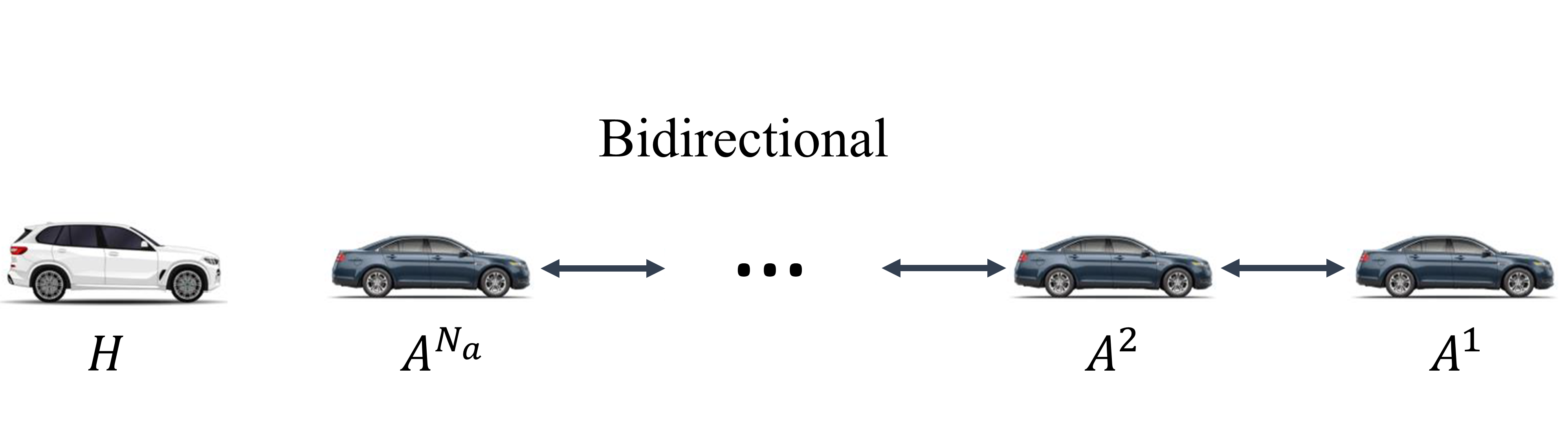
Figure 1: A mixed vehicle platoon consists of $N_{a}$ connected AVs denoting as ${A^{1},A^{2},\cdots,A^{N_{a}}}$, along with a HVs $H$ following at the rear. The AVs share real-time information such as speed, acceleration, and distance with a one-after-the-other bidirectional communication topology. There is no communication between the CAVs and the HV. In contrast to scenarios where an HV interacts with a single AV that lacks cooperation from the traffic in front, AVs within a platoon can coordinate their behaviors to enable a safer interaction between the following HV and the last AV in the platoon.

I-A Contributions

This paper proposes a learning-based method to model HVs interacting with a platoon of AVs for longitudinal car-following control applications. The main contributions are summarized as follows:

• We proposed a novel approach that combines a first principles-based model of human behaviors and a data-driven GP model trained on human-in-the-loop simulator data to model HVs in a velocity tracking setting. The GP model corrects and estimates the uncertainty of the velocity prediction. Our new model reduces the modeling error by 35.6% compared to the first-principles model. To improve the efficiency of the GP model (full GP), we employed a sparse GP technique to reduce the average computational time by 18 times compared to the full GP model and still provide a 24% overall modeling accuracy improvement compared to the first-principles model.

• We developed a chance-constrained MPC strategy (GP-MPC) that utilized the proposed HV model to estimate modeling uncertainties as an additional probabilistic constraint to guarantee a safe distance between the HV and the front AV. This probabilistic constraint was added to a pre-defined deterministic distance to form an adaptive safe distance constraint to ensure safer HV-AV interactions.

• Simulation studies show that the GP-MPC outperforms a baseline MPC approach (nominal MPC) which uses the first-principles model. The GP-MPC ensures a greater minimum distance between vehicles and enables more efficient travel behaviors (higher travel speeds) for all vehicles in the mixed platoon. Compared to the nominal MPC, the GP-MPC requires only 5% increase in computation time due to the use of sparse GP modeling for HV and a dynamic GP prediction in MPC. As a result, the average computation time of the GP-MPC at each time has been reduced by approximately 100 times compared to previous work [6] that did not employ these techniques.

I-B Related work

A growing number of studies have been conducted on the safe interactions between HVs and AVs in mixed traffic scenarios [7]. However, in most of these studies, human behaviors are either assumed to be the same in HV-AV interactions or uncertainties of HVs are difficult to be incorporated into the model-based control design [8]. Traditional first-principles-based models usually assume a fixed reaction delay for human drivers and identify model parameters from prior observations of a group of similar drivers to capture general driving behaviors [9]. While these models can interpret general human driving behaviors, their accuracy is limited as they are parametric and have few parameters to capture the complex behaviors of human drivers.

To overcome the limitations of fixed-form parametric models in car-following controls, researchers have explored learning-based or data-driven modeling methods. Artificial Neural Networks (ANNs), such as radial basis function networks [10], multilayer neural networks [11], and recurrent neural networks [12], have been proposed to address the instantaneous reaction delay of human drivers. Other approaches, such as Gaussian Mixture Regression [13] and Hidden Markov Model [14], have been used to handle the stochastic uncertainties of human drivers. These nonparametric methods are able to provide more accurate predictions of human drivers’ behaviors than parametric models.

In the field of learning-based robotics control, a nonparametric method, Gaussian process (GP) models have been actively applied to model complex robotic systems including physical human-robot interaction [15]. GP-based methods are popular in robotic applications because they require fewer parameters than other machine learning methods to capture complex behaviors [16]. Most importantly, a GP model can assess the uncertainties of its predictions through interpretable variances, which can be used to provide performance analysis and safety guarantees of a control system [17]. The system model is commonly represented by the sum of a fixed-form nominal model (parametric) and a GP component to learn the discrepancies between the nominal model and the true system behaviors [18]. Because the human driver’s behaviors have both deterministic and stochastic components [19], rather than utilizing either a fixed-form parametric model or a nonparametric modeling method, we model the HVs as a combination of a traditional fixed-form model and a GP learning-based model.

The paper is organized as follows. Sec. II explains the mathematical preliminaries. Sec. III proposes the new modeling method for HVs. Sec. IV develops an MPC policy utilizing the proposed HV model and presents simulation comparisons between the developed MPC and a baseline MPC strategy. Sec. V provides concluding remarks.

II PRELIMINARIES

II-A First-principles model of human-driven vehicles

The delay in reaction time is a significant human factor that impacts the performance of operators [20]. To account for the characteristics of human central nervous latencies, neuromuscular system, and other human and environmental factors, a transfer function with time delay has been formulated in [21] to model the human response as

$$G_{H}(s)\approx K\frac{1+T_{z}s}{1+2\gamma T_{w}s+T_{w}^{2}s^{2}}e^{-T_{d}s}=\frac{\dot{P}_{H}(s)}{\dot{P}_{N}(s)}\,,$$ (1)

where $\dot{P}_{H}(s)$ and $\dot{P}_{N}(s)$ represent Laplace transform of velocity of the HV $v_{k}^{H}$ and velocity of the AV in front $v_{k}^{N_{a}}$, respectively. The $T_{d}$ denotes the time delay of human drivers’ response. The parameters in $G_{H}$ can be identified by the collected data.

By applying a Padé approximation (second order) of the time delay component in the transfer function (1), a difference equation of the Auto-Regressive with Exogenous input (ARX) model can be derived from the discretized transfer function as [6]

$$v^{H}_{k} =-c_{1}v^{H}_{k-1}-c_{2}v^{H}_{k-2}-c_{3}v^{H}_{k-3}-c_{4}v^{H}_{k-4}$$

$$\,\quad+b_{1}v^{N_{a}}_{k-1}+b_{2}v^{N_{a}}_{k-2}+b_{3}v^{N_{a}}_{k-3}+b_{4}v^{N_{a}}_{k-4}\,,$$

$$={f}\left(v_{k-1:k-4}^{H},{v}_{k-1:k-4}^{N_{a}}\right)\,.$$ (2)

Here, $v^{H}_{k-i}$ and ${v}^{N_{a}}_{k-i}$ represent the velocity of the HV and the velocity of the last vehicle in the AV platoon at time step $k-i$, respectively.

II-B Gaussian process regression

Consider $m$ input data points $\mathbf{a}=[\mathbf{a}_{1},\cdots,\mathbf{a}_{m}]^{\mathsf{T}}\in\mathbb{R}^{n_{a}\times m}$ and the corresponding measurements $\mathbf{d}=[\mathbf{d}_{1},\cdots,\mathbf{d}_{m}]^{\mathsf{T}}\in\mathbb{R}^{n_{d}\times m}$, related through an unknown function $\mathbf{d}_{k}=\mathbf{g}(\mathbf{a}_{k})+\bm{\omega}_{k}$: $\mathbb{R}^{n_{a}}\rightarrow\mathbb{R}^{n_{d}}$, where $\bm{\omega}_{k}$ is i.i.d. Gaussian noise with $\bm{\omega}_{k}\sim\mathcal{N}(0,\bm{\Sigma^{\omega}})$ and $\bm{\Sigma^{\omega}}=\operatorname{diag}([\sigma_{1}^{2},\cdots,\sigma_{n_{d}}^{2}])$. The function $\mathbf{g}(\cdot)$ can be identified by the observed input-output dataset

$$\mathcal{D}_{m}=\{\mathbf{a} =[\mathbf{a}_{1},\cdots,\mathbf{a}_{m}]^{\mathsf{T}},\mathbf{d} =[\mathbf{d}_{1},\cdots,\mathbf{d}_{m}]^{\mathsf{T}}\}\,.$$ (3)

Assume each output dimension of $\mathbf{d}_{k}$ is independent of each other given the input $\mathbf{a}_{k}$. For each dimension $M\in\{1,\cdots,n_{d}\}$ of the function output $\mathbf{d}_{k}$, specifying a GP with zero mean and prior kernel $k^{M}(\cdot,\cdot)$, the measurement data $[\mathbf{d}_{k}]_{M,\>\cdot}$ is normally distributed as $[\mathbf{d}_{k}]_{M,\>\cdot}\sim\mathcal{N}\left(0,K_{\mathbf{a}\mathbf{a}}^{M}+\sigma_{M}^{2}\right)$, where $K_{\mathbf{a}\mathbf{a}}^{M}$ is the Gram matrix of the data points using the kernel function $k^{M}(\cdot,\cdot)$ on the input locations $\mathbf{a}$, i.e. $[K_{\mathbf{a}\mathbf{a}}^{M}]_{ij}=k^{M}(\mathbf{a}_{i},\mathbf{a}_{j})$. The choice of kernel functions $k^{M}(\cdot,\cdot)$ is specified by prior knowledge of the observed data. In the output dimension $M$, the joint distribution of the observed output $[\mathbf{d}]_{M,\>\cdot}$ and the prediction output $[\mathbf{d}]_{M}$ at new data points $a$ is $P\left([\mathbf{d}]_{M,\>\cdot},[\mathbf{d}]_{M}\,|\,\mathbf{a},a\right)$:

$$\begin{bmatrix}[\mathbf{d}]_{M,\>\cdot}\\ [\mathbf{d}]_{M}\end{bmatrix}\sim\mathcal{N}\left(0,\begin{bmatrix}K_{\mathbf{a}\mathbf{a}}^{M}+I\sigma_{M}^{2}&K_{\mathbf{a}{a}}^{M}\\ K_{{a}\mathbf{a}}^{M}&K_{{a}{a}}^{M}\end{bmatrix}\right)\,,$$ (4)

where $[K_{\mathbf{a}{a}}^{M}]_{j}=k^{M}(a_{j},a)$, $K_{{a}\mathbf{a}}^{M}=(K_{\mathbf{a}{a}}^{M})^{\mathsf{T}}$, and $K_{{a}{a}}^{M}=k^{M}(a,a)$. The posterior distribution of $[\mathbf{d}]_{M}$ conditioned on the observed data can be derived from (4) as $P\left([\mathbf{d}]_{M}\,|\,[\mathbf{d}]_{M,\>\cdot},\mathbf{a},a\right)=\mathcal{N}\left(\mu^{M}(a),\Sigma^{M}(a)\right)$ by following equations in [22]

$$\mu^{M}(a) =K_{{a}\mathbf{a}}^{M}\left(K_{\mathbf{a}\mathbf{a}}^{M}+I\sigma_{M}^{2}\right)^{-1}[\mathbf{d}]_{M,\>\cdot}\,,$$ (5a)

$$\Sigma^{M}(a) =K_{{a}{a}}^{M}-K_{{a}\mathbf{a}}^{M}\left(K_{\mathbf{a}\mathbf{a}}^{M}+I\sigma_{M}^{2}\right)^{-1}K_{\mathbf{a}{a}}^{M}\,.$$ (5b)

The resulting GP model estimation $\mathbf{d}(\cdot)$ of the unknown function $\mathbf{g}(\cdot)$ is obtained by vertically concatenating the individual output dimension $M\in\{1,\cdots,n_{d}\}$ as

$$\mathbf{d}(a)\sim\mathcal{N}\left(\bm{\mu}^{\mathbf{d}}(a),\bm{\Sigma}^{\mathbf{d}}(a)\right)\,,$$ (6)

with $\bm{\mu}^{\mathbf{d}}(a)=[\mu^{1}(a),\cdots,\mu^{n_{d}}(a)]^{\mathsf{T}}\in\mathbb{R}^{n_{d}}$ and $\bm{\Sigma}^{\mathbf{d}}(a)=\operatorname{diag}\left([\Sigma^{1}(a),\cdots,\Sigma^{n_{d}}(a)]^{\mathsf{T}}\right)\in\mathbb{R}^{n_{d}\times n_{d}}$.

II-C Sparse GP

Equations (5a) and (5b) require training data to construct the predictive distribution for each new data point prediction. The computational complexity of the mean and variance is $\mathcal{O}(n_{d}n_{a}m)$ and $\mathcal{O}(n_{d}n_{a}m^{2})$, respectively, and increases with the number of training data points $m$ [17]. As a result, the standard or vanilla GP models (6) are not suitable for applications with large datasets, such as model-based control of complex robotic systems in this study.

To reduce the computational complexity of standard GP models while maintaining reasonable approximation accuracy, several sparse spectrum approximation methods have been proposed. These methods use a subset of the dataset to approximate the kernel matrix. Specifically, given the dataset $\mathcal{D}_{m}$ of (3), the task is to select a subset $\mathbf{a}^{\text{ind}}=[\mathbf{a}_{1}^{\text{ind}},\cdots,a^{\text{ind}}_{\tilde{m}}]^{\mathsf{T}}\subset\mathbf{a}$ and $\mathbf{d}^{\text{ind}}=[\mathbf{d}^{\text{ind}}_{1},\cdots,\mathbf{d}^{\text{ind}}_{\tilde{m}}]^{\mathsf{T}}\subset\mathbf{d}$ to compute the Gaussian processes on the subset. These “pseudo inputs” $\{\mathbf{a}_{\text{ind}},\mathbf{d}_{\text{ind}}\}$ are referred to as inducing variables and $\tilde{m}$ represents the number of inducing variables. The main concept is to compress the information contained in the training data into inducing variables, which allows us to store only the inducing variables rather than the complete dataset. One state-of-the-art method, the fully independent conditional (FIC) approximation [23], automatically determines the locations of these subset inputs $\mathbf{a}_{\text{ind}}$ by optimizing gradient ascent of the GP marginal likelihood, which is convenient and has been successfully used to achieve efficient modeling of HVs in the current work.

III LEARNING-BASED MODELING OF HUMAN-DRIVEN VEHICLES

III-A The proposed modeling method for HVs

Although HVs can be modeled as an ARX model in (2) with limited accuracy by assuming a fixed reaction delay [9], incorporating GP models can improve prediction accuracy and provide uncertainty estimations that can be used as constraints for safety guarantees in control. Therefore, we propose modeling HVs in an ARX+GP format as

$$v^{H}_{k} =\sum_{i=1}^{4}c_{i}v^{H}_{k-i}+\sum_{i=1}^{4}b_{i}v^{N_{a}}_{k-i}={f}(\cdot)\quad\text{ (see \ref{eqn:arx})}\,,$$ (7a)

$$\tilde{v}^{H}_{k} =\overbrace{v^{H}_{k}}^{\text{ARX prediction}}+\overbrace{{g}(v^{H}_{k-1},v^{N_{a}}_{k-1})}^{\text{GP-based correction}}\,.$$ (7b)

Here, $\tilde{v}^{H}_{k}$ denotes the GP-compensated velocity prediction of the HV. The model ${f}(\cdot)$ is the ARX nominal model with constant parameters $b_{i}$ and $c_{i}$, and ${g}(\cdot)$ represents a GP model used to learn the discrepancies between the nominal ARX model and the actual system model (as observed through system behavior data). The GP model ${g}(\cdot)$ is a function of both the velocity of the HV ($v^{H}$) and the velocity of the AV in front of the HV ($v^{N_{a}}$).

III-B GP model training

With (7b), by using data points from previously collected measurements of velocity states $v^{H}_{j}$ and $v^{N_{a}}_{j}$, the system discrepancies are estimated by a GP model ${d}(\cdot)$ as

$${d}_{j-1}=\tilde{v}^{H}_{j}-{v}^{H}_{j}={g}({a}_{j-1})\,,$$ (8)

where the discrepancy state is defined as ${a}_{j-1}=(v^{H}_{j-1},v^{N_{a}}_{j-1})$. The $\tilde{v}^{H}_{j}$ and $v^{H}_{k}$ represent measured velocities in the previously collected data and predictive velocities derived by the nominal ARX model (7a), respectively.

In each experiment, the collected one-dimensional input-output data at all time steps are prepared by (8) as a discrepancy data set $\mathcal{D}_{m}=\{\mathbf{a}=[{a}_{1},\cdots,{a}_{j-1},\cdots,{a}_{m}]^{\mathsf{T}},\mathbf{g}=[{g}_{1},\cdots,{g}_{j-1},\cdots,{g}_{m}]^{\mathsf{T}}\}$, with $m$ being the total time steps in an experiment. The training/estimation of GP models is the process of optimizing the hyperparameters of the kernel functions, which are determined by maximizing the log marginal likelihood of collected disturbance observation data using a gradient ascent algorithm [22]. In this work, we used the squared exponential kernel like many other GP learning-based robotic control applications [17],

$$K^{M}(\mathbf{a},a)=\sigma_{f,M}^{2}\exp\bigg{(}-\frac{1}{2}\left(\mathbf{a}-a\right)^{\mathsf{T}}L_{M}^{-1}(\mathbf{a}-a)\bigg{)}\,,$$ (9)

where $\mathbf{a}$ and $a$ represent the observed points and new data points where predictions are made respectively, $\sigma_{f,M}^{2}$ and $L_{M}\in\mathbb{R}^{n_{a}\times n_{a}}$ are hyperparameters that are optimized by the log marginal likelihood function. The GP models with the optimized hyperparameters are the trained models using the observed dataset [16].

III-C Human-driven vehicle model

To estimate the HV model, we collected data from three distinct driving scenarios in which three drivers followed a platoon of AVs within a Unity simulation environment, as shown in Fig. 2. During each experiment, the drivers were intentionally distracted by performing a cognitive task involving multiple-choice algebra questions while following the platoon of AVs. We focused on investigating human behavior modeling in distracted driving scenarios because such situations present a significant challenge for ensuring safe control in AV-HV interactions, mainly due to the increased uncertainty in the HV model. The detailed steps of the data collection experiments can be found in [9, Sec. V.B]. The collected data were processed to calculate the mean values of all data points, and the calculated mean values were then used to identify the transfer function of (1). By following (2), the parameters of the ARX nominal model (2) were calculated as $c_{1}=-3.0227$, $c_{2}=3.3543$, $c_{3}=-1.6329$, $c_{4}=0.3014$, $b_{1}=0.0063$, $b_{2}=-0.0303$, $b_{3}=0.0495$, and $b_{4}=-0.0254$.

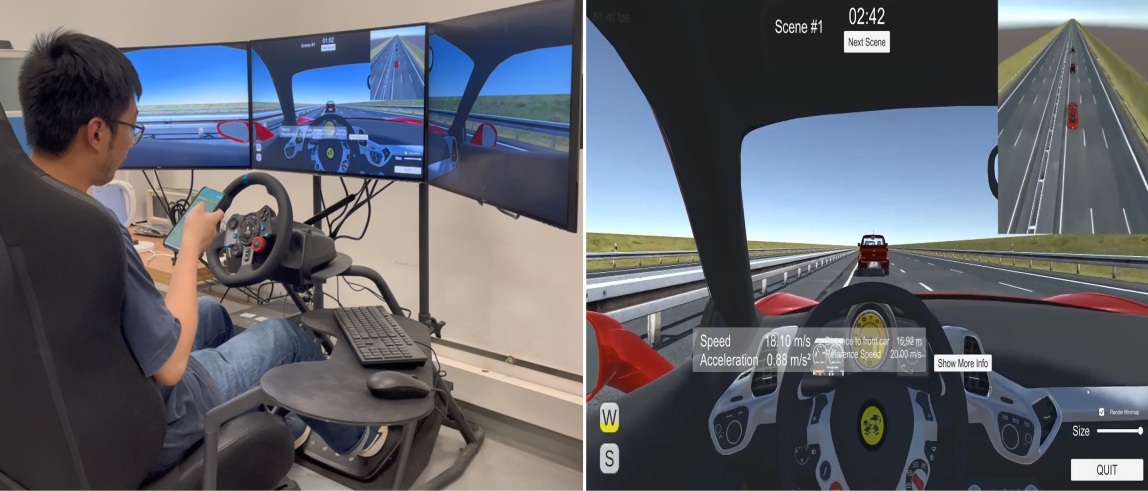
Figure 2: Data collection in a Unity driving simulator by three distracted drivers in three different driving scenarios. In each experiment, the human driver was instructed to follow a platoon of two AVs. The collected data was used for HV model identification.

We used (8) to prepare data for estimating the discrepancy between the identified ARX model in (2) and the actual HV behavior data. We trained a GP model using 20% of the data points evenly selected from six data sets, while three data sets were reserved for testing. There are two main reasons to use a partial amount of data for training the GP model. Firstly, the computational cost of using the ARX+GP model in the human-in-loop platooning control is high. More importantly, the currently collected data is not diverse, with the majority of data points occurring at velocities of 10 m$/$s, 15 m$/$s, and 20 m$/$s. As a result, we found that using a larger number of data points did not obviously improve the performance of the GP models due to the limited diversity of the data.

After the GP model was trained, we performed tests using the remaining three data sets. We plotted the velocity prediction results of the ARX model and the ARX+GP model, along with two times the standard deviation (2$\sigma$) estimated by the GP model in Figure 3. The actual measured velocities of the HV were also included in the plot to demonstrate the accuracy improvement achieved with the GP model.

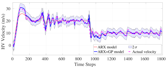
(a)

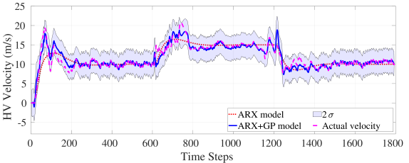
(b)

(c)

Figure 3: Performance results of the trained GP model evaluated on the three testing datasets. To compare the velocity prediction results of the ARX model and the ARX+GP model, they are plotted together with the actual measured velocities of the HV, as well as two times the standard deviation (2$\sigma$) estimated by the GP model. The plots clearly indicate that the ARX+GP model provides a significant improvement in fitting the actual velocity curves compared to the ARX model alone. Compared to the nominal ARX model, the ARX+GP model improves the modeling accuracy by an average of 35.64% in terms of root mean square error.

To quantify the accuracy improvement, the root mean square error (RMSE) was calculated for each testing data set using

$$\text{RMSE}_{{v}^{H}_{*}}=\sqrt{\sum_{i=1}^{n}\frac{\left({v}^{H}_{*}-{v}^{H}_{\text{act}}\right)^{2}}{n}}\,,$$ (10)

where ${v}^{H}_{*}$ represents the velocity predictions of either the ARX model or GP+ARX model over $n$ samples in a testing data set, and ${v}^{H}_{\text{act}}$ denotes the actually measured velocities. The RMSE calculates the mean value of the model prediction errors on each testing data set, thus lower RMSE values indicate that the model provides more accurate modeling of the HVs. We calculated the average values of the RMSE of the ARX model and GP+ARX model with three testing data set, the average RMSE of the ARX model is 1.88, and the average RMSE of the ARX+GP model is 1.21. The ARX+GP model gains an approximate 35.64% overall modeling accuracy improvement compared to the ARX model. In Fig. 3, the improved modeling accuracy can also be directly viewed as the ARX+GP model fits the curves of the actual velocity data much better than the ARX model. This is especially true for the time steps during 200$-$600, 800$-$1200, and 1400$-$1800 when the velocities are around 10 m$/$s or 15 m$/$s, which have similar velocity profiles as the training data points.

III-D Sparse GP+ARX model

We have utilized the FIC sparse approximation technique for the GP model in order to speed up the prediction process, as described in Section II-C. The hyperparameters of the sparse GP model were obtained from the trained full GP models as explained in Section III-C, and 20 inducing points were automatically selected by the FIC method within the training data sets. To evaluate the performance of the sparse GP model, we tested it on three testing data sets. The average prediction time was reduced to 0.00021s, which is approximately 18 times faster than the standard full GP model that took 0.0037s to complete each prediction.

We have included a plot of one of the three testing results of the sparse GP+ARX model (on the bottom testing data set shown in Fig. 3) in Fig. 4. In this plot, we have plotted the velocity predictions of the ARX model, the ARX+GP model, and the sparse GP+ARX model together. We observed that the sparse GP+ARX model was also able to fit the actual velocity data curves much better than the ARX model. Moreover, by utilizing (10), we calculated the average RMSE of the sparse GP+ARX model to be 1.43, indicating an approximate 23.94% overall modeling accuracy improvement when compared to the ARX model. These results indicate that the sparse GP+ARX model provides a good balance between modeling accuracy and significant computational efficiency improvement.

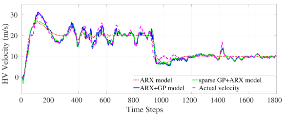
Figure 4: Performance results of the sparse GP model evaluated on one of three testing datasets. To compare the velocity prediction results of the sparse GP+ARX model, ARX+GP model, and ARX model, they are plotted together with the actual measured velocities of the HV. The sparse ARX+GP model still fits significantly better to the actual velocity curves compared to the ARX model with an average of 23.94% accuracy improvement.

IV CONTROLLER DESIGN

To further show the effectiveness of the proposed modeling approach for HVs, we designed a model predictive control strategy utilizing the proposed HV model to demonstrate its effectiveness in improving performance and safety in a mixed vehicle platoon control scenario.

IV-A System model

Consider a mixed platoon of AVs and one HV, denoted by $A^{n_{a}}$ and $H$ respectively, with $n_{a}=\{1,2,\cdots,N_{a}\}$ and $N_{a}$ represents the number of AVs shown in Fig. 1. The position and velocity of $A^{n_{a}}$ at the current time step $k$ are denoted by $p^{n_{a}}_{k}$ and $v^{n_{a}}_{k}$, respectively. We consider the following kinematic model for the AVs as

$$v_{k+1}^{n_{a}} =v_{k}^{n_{a}}+T\,\mathrm{a}_{k}^{n_{a}}\,,$$ (11a)

$$p_{k+1}^{n_{a}} =p_{k}^{n_{a}}+T\,v_{k}^{n_{a}}\,.$$ (11b)

Here $0<T\ll 1$ is the sample time, and $\mathrm{a}_{k}^{n_{a}}$ represents the acceleration of $A^{n_{a}}$. We assume autonomous vehicles are deterministic and can measure (and communicate) their states without any error, i.e., $\Sigma(v_{k}^{n_{a}})=0$.

By applying (7b), the human-driven vehicle model is

$$\tilde{v}_{k}^{H} =v_{k}^{H}+{d}(v_{k-1}^{H},{v}_{k-1}^{N_{a}})\,,$$ (12a)

$$p_{k+1}^{H} =p_{k}^{H}+T\,\tilde{v}_{k}^{H}\,,$$ (12b)

Here, $\tilde{v}_{k}^{H}$ represents the GP compensated HV velocity, the $v_{k}^{H}$ (computed via (2)) and $p_{k}^{H}$ are the velocity and position states at the current time step $k$ respectively, thus the variance $\Sigma(v_{k}^{H})=0$ and $\Sigma(p_{k}^{H})=0$. Applying (6), the propagation equation for the mean of position is derived as

$$\mu_{k+1}^{p^{H}} =\mu_{k}^{p^{H}}+T\,v_{k}^{H}+T\,\mu^{d}(v_{k-1}^{H},{v}_{k-1}^{N_{a}})\,,$$ (13)

with the initial value $\mu_{0}^{p^{H}}=p_{k}^{H}$. The propagation equation for the variance of position is

$$\Sigma\left(p_{k+1}^{H}\right) =\Sigma\left(p_{k}^{H}+T\,v_{k}^{H}+T\,{d}(v_{k-1}^{H},{v}_{k-1}^{N_{a}})\right)\,,$$ (14a)

$$=\Sigma_{k}^{p^{H}}+T^{2}\Sigma^{d}_{k-1}\ ,$$ (14b)

with the initial value $\Sigma\left(p_{0}^{H}\right)=0$. The equation (14b) neglects the covariance between $p_{k}^{H}$ and $v_{k}^{H}$.

IV-B Safe distance chance constraint

To guarantee a safe distance between vehicles in the mixed platoon, a constraint of distance between AVs is designed with a constant value $\Delta$ as $p_{k}^{n_{a}-1}-p_{k}^{n_{a}}>\Delta$. Due to the stochastic feature of the HV model, a chance constraint of the distance between the last AV and the HV is designed to be satisfied as

$$\mathrm{Pr}\left(p_{k}^{N_{a}}-(p_{k}^{H}+\Delta)>\Delta_{\text{ext}}\right)\geq p_{\text{def}}\,,$$ (15)

where $\Delta$ is the defined safe distance between AVs, and $\Delta_{\text{ext}}\geq 0$ represents an additional distance to compensate for the stochastic nature of the HVs. The satisfaction probability is denoted by $p_{\text{def}}$. We can reformulate the distance constraint $\mathcal{X}$ following a single half-space constraint $\mathcal{X}^{hs}:=\bigl{\{}x|h^{\top}x\leq b\bigl{\}}$, $h\in\mathbb{R}^{n}$, $b\in\mathbb{R}$. In [17], a method of tightened constraint on the state mean is derived as

$$\mathcal{X}^{hs}\left(\Sigma_{i}^{x}\right):=\left\{x\mid h^{\top}x\leq b-\phi^{-1}\left(p_{\text{def}}\right)\sqrt{h^{\top}\Sigma_{i}^{x}h}\right\}\,,$$ (16)

where $h^{\top}=\begin{bmatrix}-1&1\end{bmatrix}$, $x:=\begin{bmatrix}p_{k}^{N_{a}}&p_{k}^{H}+\Delta\end{bmatrix}^{\top}$, and $b=-\Delta_{\text{ext}}$. The $\phi^{-1}$ represents the inverse of the cumulative distribution function (CDF). In our case,

$$\Sigma_{k}^{x}:=\begin{bmatrix}\Sigma_{k}^{p^{N_{a}}}\\ \Sigma_{k}^{p^{H}}+\Delta\end{bmatrix}=\begin{bmatrix}0&0\\ 0&\Sigma_{k}^{p^{H}}\end{bmatrix}\,.$$ (17)

Here, there is no covariance between the position states of the last AV and the HV and $\Sigma_{k}^{p^{N_{a}}}=0$. The position variance of the human-driven vehicle $\Sigma_{k}^{p^{H}}$ is calculated using (14b). To obtain a “tightened” position constraint, (16) is substituted with (17) to obtain

$$p_{k}^{N_{a}}-p_{k}^{H}\geq\Delta+\Delta_{\text{ext}}+\phi^{-1}\left(p_{\text{def}}\right)\sqrt{\Sigma_{k}^{p^{H}}}\,.$$ (18)

The chance constraint of safe distance defined in (15) is approximated as a deterministic equation given by (18). The extra component $\Delta_{\text{ext}}$ can be set to $0$ if a high satisfaction probability value is used for further approximation. The safe distance constraint between the HV and AVs is adaptively modified based on the uncertainty estimates of the HV by the GP model. The modified safe distance constraint is ensured to be greater than $\Delta$ at all times.

IV-C GP learning-based model predictive control

A GP learning-based MPC (GP-MPC) strategy for the longitudinal car-following control of a mixed vehicle platoon comprising $N_{a}$ number of AVs and one HV shown in Fig. 1 is developed as

$$\underset{\mathbb{V}}{\text{min}}\sum_{n^{a}=1}^{N_{a}} \sum_{i=k}^{k+N-1}\Big{\|}a_{{i}|k}^{n_{a}}\Big{\|}^{2}_{R}+\sum_{i=k}^{k+N}\Big{\|}v_{{i+1}|k}^{1}-v_{{i+1}|k}^{\text{ref}}\Big{\|}^{2}_{Q_{1}}$$

$$\qquad\quad+\sum_{n^{a}=2}^{N_{a}}\sum_{i=k}^{k+N}\Big{\|}v_{{i+1}|k}^{n_{a}}-v_{{i+1}|k}^{n_{a}-1}\Big{\|}^{2}_{Q_{2}}$$ (19a)

$$\text{with}\ \mathbb{V}= \left\{v_{{i}|k}^{1},v_{{i}|k}^{n_{a}},v_{{i}|k}^{H},p_{{i}|k}^{n_{a}},\mu_{{i}|k}^{p^{H}},\Sigma_{{i}|k}^{p^{H}},a_{{i}|k}^{n_{a}}\right\}\,$$

subject to

$$v_{{i+1}|k}^{n_{a}} =v_{{i}|k}^{n_{a}}+T\,\mathrm{a}_{{i}|k}^{n_{a}},\ p_{{i+1}|k}^{n_{a}}=p_{{i}|k}^{n_{a}}+T\,v_{{i}|k}^{n_{a}}\,,$$ (19b)

$$v^{H}_{{i}|k} ={f}\left(v_{i-1:i-4|k}^{H},{v}_{i-1:i-4|k}^{N_{a}}\right)\,,$$ (19c)

$$\mu_{{i+1}|k}^{p^{H}} =\mu_{{i}|k}^{p^{H}}+T\,v_{{i}|k}^{H}+T\,\mu^{d}(v_{{i-1}|{k}}^{H},{v}_{{i-1}|{k}}^{N_{a}})\,,$$ (19d)

$$\Sigma_{{i+1}|k}^{p^{H}} =\Sigma_{{i}|k}^{p^{H}}+T^{2}\Sigma^{d}(v_{{i-1}|{k}}^{H},{v}_{{i-1}|{k}}^{N_{a}})\,,$$ (19e)

$$p_{{i}|k}^{n_{a}-1} -p_{{i}|k}^{n_{a}}\geq\Delta\,,$$ (19f)

$$p_{{i}|k}^{N_{a}} -\mu_{{i}|k}^{p^{H}}\geq\Delta+\phi^{-1}\left(p_{\text{def}}\right)\sqrt{\Sigma_{{i}|k}^{p^{H}}}\,,$$ (19g)

$$v_{\text{min}} \leq v_{{i}|k}^{n_{a}}\leq v_{\text{max}}\,,\ a_{\text{min}}\leq a_{{i}|k}^{n_{a}}\leq a_{\text{max}}\,.$$ (19h)

The current time step is $k$, and the system (hardware or simulation) starts at time $k=0$. In the MPC prediction horizon, the prediction horizon time step starts at $i=1$, and variable values at $i=0$ are initialized with measurements [6]. In the cost function (19a), differences between the reference velocity and velocity of the leading AV, differences between velocities of the neighboring AVs, and control inputs are weighted by three positive weights $Q_{1}$, $Q_{2}$, and $R$ repetitively. In the equality constraint (19b)$-$(19e), the (19b) are the model of AVs defined in (11a) and (11b), the (19c) is the ARX nominal model of the HV specified in (2), the (19d) and (19e) are mean and variance propagation equations of the HV position derived in (13) and (14b) respectively. The inequality constraints include the velocity and acceleration (19h), and safe distance (19f) and (19g).

IV-D Dynamic sparse GP prediction in MPC

In Section III-D, it was demonstrated that the sparse GP+ARX model significantly reduces computation time (compared to the standard GP+ARX model) while still improving modeling accuracy (compared to the ARX model) for HV velocity predictions. However, integrating GP models into the MPC framework to achieve a reasonable speed or real-time calculations remains a challenge. MPC itself is computationally expensive as it requires solving an optimal control problem at each time step while satisfying constraints specified in equations (19b)$-$(19h). To address this challenge, we implemented a dynamic sparse approximation for the GP-MPC method proposed in [17] to achieve further speed-up. Given the receding horizon feature of MPC, the predictive trajectory at the current time step is similar to the trajectory calculated at the previous time step. Therefore, we applied the sparse GP to conduct calculations on the trajectory at the previous time step and used the results to propagate the mean and variance at the current time step by using (19d) and (19e).

IV-E Simulations

This section shows the overall control performance improvement due to utilizing the proposed HV model. A simulation case study of the mixed vehicle platoon applying the sparse GP-based MPC strategy developed in Sec. IV-C and a baseline MPC were quantitatively compared. All simulations were implemented in MATLAB R2022a on a laptop computer running Ubuntu 20.04. The source code for our implementation is available at: https://github.com/CL2-UWaterloo/GP-MPC-of-Platooning.

To ensure consistent starting conditions across all simulations, the initial velocities of all vehicles were set to 0. We used a sample time of T = 0.25 s and a prediction horizon of N = 6 for both the baseline MPC and the sparse GP-based MPC. The weights of the cost function for both MPC policies were tuned to $Q_{1}=Q_{2}=5$ and $R=20$. The maximum and minimum acceleration were set to $a_{\text{max}}=$ 5 m${}^{2}/$s and $a_{\text{min}}=$ $-$5 m${}^{2}/$s respectively, and the maximum and minimum velocity were set to $v_{\text{max}}=$ 35 m$/$s and $v_{\text{min}}=$ $-$35 m$/$s respectively. The minimum safe distance was defined as $\Delta=$ 20 m in (19f) and (19g). We initialized the leader AV at $p=0$, the second AV was $1.2\,\Delta=$ 24 m behind the leader AV, and the HV was located $1.2\,\Delta=$ 24 m behind the follower AV. The satisfaction probability of the chance constraint in (15) was set to $p_{\text{def}}=0.95$.

We implemented a baseline MPC, referred to as the nominal MPC, to provide a basis for comparison. In the nominal MPC, the prediction loop uses the ARX model of the HV (19c) and (19d) without the third GP component. The distance constraint between the HV and the follower AV given is defined as $\Delta$ without the second adaptive component in (19g). Furthermore, the nominal MPC does not incorporate position variance propagation as described in equation (19e). For all simulations involving the nominal MPC and the sparse GP-based MPC, we utilized the ARX+GP model derived in equations (12a) and (12b) to simulate the HV model.

A case study of emergency braking was simulated by applying the nominal MPC and GP-MPC. Specifically, we simulated the scenario with a reference velocity of $v^{\text{ref}}=$ 20 m$/$s for the leading AV, which was then reduced to $v^{\text{ref}}=$ 10 m$/$s at $t=$ 30 s. We then plotted the velocity tracking, position of each vehicle, and relative distance between the vehicles, shown from top to bottom in Fig. 5 for the nominal MPC and in Fig. 6 for the GP-MPC.

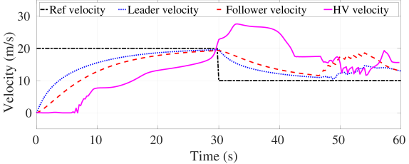
(a)

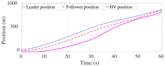
(b)

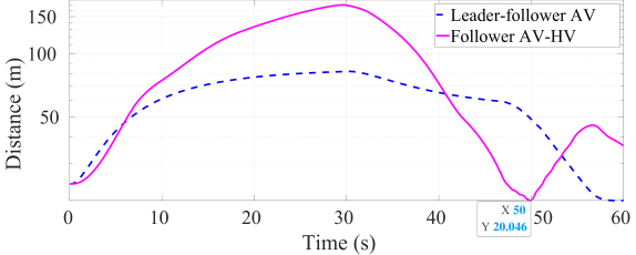
(c)

Figure 5: Simulation results of an emergency braking scenario with a baseline MPC for the mixed vehicle platoon control. From top to bottom, the plots are the velocity tracking, the position of each vehicle, and the relative distance between vehicles respectively.

(a)

(b)

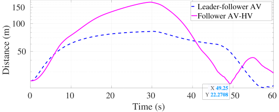
(c)

Figure 6: Simulation results of an emergency braking scenario with the proposed GP-MPC for the mixed vehicle platoon control. The plots show the velocity tracking, position of each vehicle, and relative distance between vehicles from top to bottom, respectively. Compared to a baseline MPC shown in Fig. 5, the minimum distance between the HV and follower AV is two-meter larger, and the traveled distances of all vehicles are larger as summarized in Tab. I. Therefore, the GP-MPC approach offers better safety guarantees without being more conservative than the nominal MPC since all vehicles still travel a larger distance.

The top plots of the velocity tracking demonstrate the cooperative maneuvers of the leader and follower AVs. At around $t=$ 46 s, both AVs accelerated to guarantee the safe distance constraint.

We summarized the position of the leader AV (AV 1), the follower AV (AV 2), and the HV (HV) as well as the minimum distance between the HV and the follower AV (Min HV-AV) in Tab. I to quantitatively show the performance improvements of the proposed GP-MPC. The GP-MPC achieved a minimum HV-AV distance of 22.27 m, which is two meters larger than the nominal MPC. This improvement is due to the additional component in the safe distance constraint that considers the GP uncertainty assessments defined in (18). Extra distances were added to the distance constraint in (19g) at all time steps in the GP-MPC to better guarantee safety. All the vehicle positions in the mixed platoon of the GP-MPC were ahead of the nominal MPC, this indicates the GP-MPC also realized a higher travel speed for all vehicles in the mixed-vehicle platoon.

TABLE I: Simulation performance metrics: The position of all vehicles and the minimum relative distance of HV-AV.

Controller	AV 1	AV 2	HV	Min HV-AV
Nominal MPC	862.90 m	842.89 m	806.42 m	20.05 m
GP-MPC	864.92 m	843.72 m	814.60 m	22.27 m

We also summarized the computation time at each time step of the GP-MPC and the nominal MPC in Table II. The average computation time (Ave Time) of the MPC at each time step for the GP-MPC is only 5% more than the nominal MPC. The maximum time (Max Time) of the GP-MPC shows it can run in real-time at 4 HZ, and the small standard deviation (Time Std) value of the GP-MPC indicates it has a more consistent computation time than the nominal MPC. Compared to our previous work [6] that did not utilize sparse GP modeling for HVs and a dynamic GP prediction in MPC, the average computation time of the GP-MPC at each time step has been reduced by approximately 100 times.

TABLE II: Simulation computation time: The averaged time at each time step of the GP-MPC is only 5% more than the nominal MPC.

Controller	Ave Time	Max Time	Time Std
Nominal MPC	0.2062 s	0.2347 s	0.065
GP-MPC	0.2186 s	0.2391 s	0.006

V CONCLUSIONS

Summary. This paper proposes an innovative learning-based modeling approach for human-driven vehicles that combines a first-principles nominal model with a Gaussian process learning-based component. The proposed model improves the modeling accuracy and estimates the uncertainty in the HV model, thus can be used to enhance the safe control of mixed vehicle platoon. Utilizing this model, we developed a model predictive control strategy for a mixed vehicle platoon in longitudinal car-following scenarios. We evaluated the developed MPC policy by comparing it to a baseline MPC in simulation case studies. The results show that our approach achieves superior safety guarantees while also enabling more efficient motion behaviors for all vehicles in a mixed platoon. By utilizing a dynamic sparse GP technique in every MPC prediction loop, our MPC requires only 5% more computation time than the baseline nominal MPC, which represents an approximately 100-fold reduction in computation time compared to our previous work [6].

Limitations and future work. Our work is limited in many ways. Firstly, it is important to note that our current work is limited to longitudinal car-following scenarios, and it would be beneficial to expand it to other traffic scenarios such as merging or lane changing. Secondly, Although the GP models were trained with data from real human drivers, the limited diversity of the data collected to model human-driven vehicles suggests that gathering more data from diverse drivers and driving scenarios could further enhance the model’s accuracy. Finally, further investigation is required to establish the minimum distance constraint necessary for the proposed GP-MPC to ensure safe control. Exploring the method’s boundary capabilities represents an exciting area for future research.

References

- [1] J. Guanetti, Y. Kim, and F. Borrelli, “Control of connected and automated vehicles: State of the art and future challenges,” Annual reviews in control, vol. 45, pp. 18–40, 2018.
- [2] M. Martínez-Díaz, C. Al-Haddad, F. Soriguera, and C. Antoniou, “Platooning of connected automated vehicles on freeways: a bird’s eye view,” Transportation research procedia, vol. 58, pp. 479–486, 2021.
- [3] Y. Rahmati, M. Khajeh Hosseini, A. Talebpour, B. Swain, and C. Nelson, “Influence of autonomous vehicles on car-following behavior of human drivers,” Transportation research record, vol. 2673, no. 12, pp. 367–379, 2019.
- [4] P. Dorde, M. Radomir, and D. Pesic, “Traffic accidents with autonomous vehicles: type of collisions, manoeuvres and errors of conventional vehicles’ drivers,” Transportation research procedia, vol. 45, pp. 161–168, 2020.
- [5] A. Sadat, S. Casas, M. Ren, X. Wu, P. Dhawan, and R. Urtasun, “Perceive, predict, and plan: Safe motion planning through interpretable semantic representations,” in European Conference on Computer Vision. Springer, 2020, pp. 414–430.
- [6] J. Wang, Z. Jiang, and Y. V. Pant, “Improving safety in mixed traffic: A learning-based model predictive control for autonomous and human-driven vehicle platooning,” arXiv preprint arXiv:2211.04665, 2023.
- [7] C. M. Tampère, “Human-kinetic multiclass traffic flow theory and modelling. With application to advanced driver assistance systems in congestion,” Ph.D. dissertation, Delft University of Technology, 2004.
- [8] L. Guo and Y. Jia, “Inverse model predictive control (IMPC) based modeling and prediction of human-driven vehicles in mixed traffic,” IEEE Transactions on Intelligent Vehicles, vol. 6, no. 3, pp. 501–512, 2020.
- [9] M. Pirani, Y. She, R. Tang, Z. Jiang, and Y. V. Pant, “Stable interaction of autonomous vehicle platoons with human-driven vehicles,” in 2022 American Control Conference (ACC). IEEE, 2022, pp. 633–640.
- [10] S. Panwai and H. Dia, “Neural agent car-following models,” IEEE Transactions on Intelligent Transportation Systems, vol. 8, no. 1, pp. 60–70, 2007.
- [11] A. Khodayari, A. Ghaffari, R. Kazemi, and R. Braunstingl, “A modified car-following model based on a neural network model of the human driver effects,” IEEE Transactions on Systems, Man, and Cybernetics-Part A: Systems and Humans, vol. 42, no. 6, pp. 1440–1449, 2012.
- [12] J. Morton, T. A. Wheeler, and M. J. Kochenderfer, “Analysis of recurrent neural networks for probabilistic modeling of driver behavior,” IEEE Transactions on Intelligent Transportation Systems, vol. 18, no. 5, pp. 1289–1298, 2016.
- [13] S. Lefevre, Y. Gao, D. Vasquez, H. E. Tseng, R. Bajcsy, and F. Borrelli, “Lane keeping assistance with learning-based driver model and model predictive control,” in 12th International Symposium on Advanced Vehicle Control, 2014.
- [14] T. Qu, S. Yu, Z. Shi, and H. Chen, “Modeling driver’s car-following behavior based on hidden markov model and model predictive control: A cyber-physical system approach,” in 2017 11th Asian Control Conference (ASCC). IEEE, 2017, pp. 114–119.
- [15] K. Haninger, C. Hegeler, and L. Peternel, “Model predictive control with gaussian processes for flexible multi-modal physical human robot interaction,” in 2022 International Conference on Robotics and Automation (ICRA). IEEE, 2022, pp. 6948–6955.
- [16] J. Wang, “An intuitive tutorial to Gaussian processes regression,” arXiv preprint arXiv:2009.10862, 2020.
- [17] L. Hewing, J. Kabzan, and M. N. Zeilinger, “Cautious model predictive control using Gaussian process regression,” IEEE Transactions on Control Systems Technology, vol. 28, no. 6, pp. 2736–2743, 2019.
- [18] J. Wang, M. T. Fader, and J. A. Marshall, “Learning-based model predictive control for improved mobile robot path following using Gaussian processes and feedback linearization,” Journal of Field Robotics, 2023.
- [19] X. Chen, L. Li, and Y. Zhang, “A markov model for headway/spacing distribution of road traffic,” IEEE Transactions on Intelligent Transportation Systems, vol. 11, no. 4, pp. 773–785, 2010.
- [20] R. Antunes, F. V. Coito, and H. Duarte-Ramos, “A linear approach towards modeling human behavior,” in Doctoral Conference on Computing, Electrical and Industrial Systems. Springer, 2011, pp. 305–314.
- [21] C. C. Macadam, “Understanding and Modeling the Human Driver,” Vehicle System Dynamics, 2003.
- [22] C. E. Rasmussen and C. K. I. Williams, Gaussian processes in machine learning. MIT Press, 2006.
- [23] E. Snelson and Z. Ghahramani, “Sparse gaussian processes using pseudo-inputs,” Advances in neural information processing systems, vol. 18, 2005.