Weakly reversible deficiency one realizations of polynomial dynamical systems: an algorithmic perspective

Abstract

Given a dynamical system with polynomial right-hand side, can it be generated by a reaction network that possesses certain properties? This question is important because some network properties may guarantee specific dynamical properties, such as existence or uniqueness of equilibria, persistence, permanence, or global stability. Here we focus on this problem in the context of weakly reversible deficiency one networks. In particular, we describe an algorithm for deciding if a polynomial dynamical system admits a weakly reversible deficiency one realization, and identifying one if it does exist. In addition, we show that weakly reversible deficiency one realizations can be partitioned into mutually exclusive Type I and Type II realizations, where Type I realizations guarantee existence and uniqueness of positive steady states, while Type II realizations are related to stoichiometric generators, and therefore to multistability.

1 Introduction

By a polynomial dynamical system we mean a dynamical system of the form

$$\begin{split}\frac{dx_{1}}{dt}&=p_{1}(x_{1},\ldots,x_{n}),\\ \frac{dx_{2}}{dt}&=p_{2}(x_{1},\ldots,x_{n}),\\ &\qquad\quad\vdots\\ \frac{dx_{n}}{dt}&=p_{n}(x_{1},\ldots,x_{n}),\\ \end{split}$$ (1)

where each $p_{i}(x_{1},\ldots,x_{n})$ is a polynomial in the variables $x_{1},\ldots,x_{n}$. Such systems can exhibit exotic behaviors like multistability, presence of oscillations, and chaos due to the underlying nonlinearities. We are especially interested in the dynamics of these systems when restricted to the positive orthant, because such systems are very common models of biological interaction networks, population dynamics models, or models for the transmission of infectious diseases [1, 2, 3, 4].

Very often, polynomial dynamical systems are generated by reaction networks. It is often convenient to study the graphical structure of these networks to make inference about their dynamics. It is also possible to study the inverse problem, i.e., for some given polynomial dynamical systems, ask what reaction networks can generate them. Due to the phenomenon of dynamical equivalence [5, 6], such a network may not be unique, i.e., there exist multiple reaction networks that generate the same dynamics.

A key quantity in the study of these networks is its deficiency. In particular, networks possessing low deficiency have been studied in reaction network theory using the Deficiency Zero and Deficiency One theorems [2, 6, 7, 8, 9, 10]. In particular, the Deficiency One Theorem [2, 10] guarantees uniqueness of the steady state within each linear invariant subspace; this, together with the existence result in [11] completely characterizes the steady states of weakly reversible networks that satisfy the hypotheses of the Deficiency One Theorem. Further, weakly reversible networks (i.e., networks where each reaction is part of a cycle) are related to dynamical properties like persistence, permanence, and the existence of a globally attracting steady state [12, 13, 14, 15].

The problem of identifying weakly reversible deficiency zero realizations has been addressed in [16]. Here we analyze the realizability problem for weakly reversible reaction networks with deficiency one. In particular, given a polynomial dynamical system, we describe an algorithm to identify if there exists a weakly reversible deficiency one reaction network that generates this dynamical system. Moreover, if weakly reversible deficiency one realizations do exist, our algorithm uses the geometry of some convex cones generated using the net reaction vectors to construct one such realization explicitly.

Structure of this paper. In Section 2, we recall some basic notions from reaction network theory. Primarily, we introduce dynamical equivalence and the matrix of net reaction vectors. In Section 3, we give a short primer on weakly reversible deficiency one reaction networks, and define Type I and Type II weakly reversible deficiency one realizations. In Section 4, we analyze the pointed cone $\text{ker}(\boldsymbol{W})\cap\mathbb{R}^{m}_{\geq 0}$ and its minimal set of generators in the context of weakly reversible deficiency one networks. Moreover, we prove there cannot exist a dynamical equivalence between such networks of two types in Theorem 4.11. In Section 5, we state the main algorithm of our paper: Algorithm 5.1, which checks the existence of a weakly reversible deficiency one realization and returns a realization if it exists. In Section 6, we summarize our findings in this paper and flesh out directions for future work.

Notation. We let $\mathbb{R}_{\geq 0}^{n}$ and $\mathbb{R}_{>0}^{n}$ denote the set of vectors in $\mathbb{R}^{n}$ with non-negative and positive entries respectively. Given two vectors $\boldsymbol{x}=(\boldsymbol{x}_{1},\ldots,\boldsymbol{x}_{n})^{\intercal}\in\mathbb{R}^{n}_{>0}$ and $\boldsymbol{y}=(\boldsymbol{y}_{1},\ldots,\boldsymbol{y}_{n})^{\intercal}\in\mathbb{R}^{n}$, we use the vector operation as follows:

$$\boldsymbol{x}^{\boldsymbol{y}}:=\boldsymbol{x}_{1}^{y_{1}}\ldots\boldsymbol{x}_{n}^{y_{n}}.$$

Given a positive integer $m$, we denote $[m]:=\{1,\ldots,m\}$.

2 Reaction networks

2.1 Terminology

Definition 2.1.

A reaction network $G=(V,E)$, also called the Euclidean embedded graph (E-graph), is a directed graph in $\mathbb{R}^{n}$, where $V\subsetneq\mathbb{R}^{n}$ represents a finite set of vertices, and $E\subseteq V\times V$ represents a finite set of edges. In this paper, there are neither self-loops nor isolated vertices in $G$.

1. Let $V=\{\boldsymbol{y}_{1},\ldots,\boldsymbol{y}_{m}\}$, and denote the number of vertices in $G$ by $m$.

2. We denote a directed edge by $(\boldsymbol{y}_{i},\boldsymbol{y}_{j})\in E$, which represents a reaction in the network. Here $\boldsymbol{y}_{i}$ and $\boldsymbol{y}_{j}$ are called the source vertex and target vertex respectively. Moreover, we denote the reaction vector associated with the edge $\boldsymbol{y}_{i}\rightarrow\boldsymbol{y}_{j}$ by $\boldsymbol{y}_{j}-\boldsymbol{y}_{i}\in\mathbb{R}^{n}$.

Definition 2.2.

Let $G=(V,E)$ be a Euclidean embedded graph. The stoichiometric subspace of $G$ is the vector space spanned by the reaction vectors as follows:

$$S=\text{span}\{\boldsymbol{y}^{\prime}-\boldsymbol{y}\,|\,\boldsymbol{y}\rightarrow\boldsymbol{y}^{\prime}\in E\}.$$

Given a subset of vertices $V_{0}\subseteq V$, the stoichiometric subspace defined by $V_{0}$ is

$$S(V_{0})=\text{span}\{\boldsymbol{y}^{\prime}-\boldsymbol{y}\,|\,\boldsymbol{y}\rightarrow\boldsymbol{y}^{\prime}\in E\ \text{and}\ \boldsymbol{y}^{\prime},\boldsymbol{y}\in V_{0}\}.$$

Furthermore, given a positive vector $\boldsymbol{x}_{0}\in\mathbb{R}_{>0}^{n}$, the polyhedron $(\boldsymbol{x}_{0}+S)\cap\mathbb{R}^{n}_{>0}$ is called the stoichiometric compatibility class of $\boldsymbol{x}_{0}$.

Definition 2.3.

Let $G=(V,E)$ be a Euclidean embedded graph.

1. The set of vertices $V$ is partitioned by its connected components, also called linkage classes. Every connected component is denoted by the set of vertices belonging to it.

2. A connected component $L\subseteq V$ is strongly connected, if every edge is part of an oriented cycle. Moreover, a strongly connected component $L\subseteq V$ is terminal strongly connected, if for every vertex $\boldsymbol{y}\in L$ and $\boldsymbol{y}\rightarrow\boldsymbol{y}^{\prime}\in E$, we have $\boldsymbol{y}^{\prime}\in L$.

3. $G=(V,E)$ is weakly reversible, if all connected components are strongly connected.

Remark 2.4.

For any weakly reversible reaction network $G=(V,E)$, every vertex $\boldsymbol{y}\in V$ is a source and a target vertex. Moreover, every connected component of $G$ is strongly connected, and terminal strongly connected.

Definition 2.5.

Let $G=(V,E)$ be a Euclidean embedded graph, which contains $m$ vertices and $\ell$ connected components. Denote the dimension of the stoichiometric subspace of $G$ by $s=\dim(S)$, the deficiency of $G$ is a non-negative integer as follows:

$$\delta=m-\ell-s.$$

When considering a linkage class with $V_{i}\subseteq V$, we define the deficiency of a linkage class as

$$\delta_{i}=|V_{i}|-1-\dim S(V_{i}).$$

One can check that

$$\delta\geq\sum_{i=1}^{\ell}\delta_{i},$$ (2)

where the equality holds when the stoichiometric subspaces of all linkage classes are linearly independent.

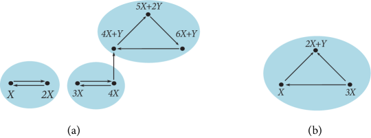
Figure 1: (a) This reaction network consists of two linkage classes and contains three terminal strongly connected components (shown in circles). It has a stoichiometric subspace of dimension 2 and a deficiency $\delta=n-\ell-s=7-2-2=3$. (b) This reaction network is weakly reversible and contains one terminal strongly connected component. It has a stoichiometric subspace of dimension 2 and a deficiency $\delta=n-\ell-s=3-1-2=0$.

Figure 1 shows two reaction networks represented as Euclidean embedded graphs. Given a reaction network, it can generate an extensive variety of dynamical systems. Here, we focus on mass-action kinetics, which has been studied in [1, 3, 4, 17, 18, 19].

Definition 2.6.

Let $G=(V,E)$ be a Euclidean embedded graph, we let $\boldsymbol{k}=(k_{\boldsymbol{y}_{i}\rightarrow\boldsymbol{y}_{j}})_{\boldsymbol{y}_{i}\rightarrow\boldsymbol{y}_{j}\in E}\in\mathbb{R}_{>0}^{E}$ denote the vector of reaction rate constants, where $k_{\boldsymbol{y}_{i}\rightarrow\boldsymbol{y}_{j}}$ or $k_{ij}$ is called the reaction rate constant of the edge $\boldsymbol{y}_{i}\rightarrow\boldsymbol{y}_{j}\in E$. Furthermore, the associated mass-action system generated by $(G,\boldsymbol{k})$ on $\mathbb{R}^{n}_{>0}$ is

$$\frac{\mathrm{d}\boldsymbol{x}}{\mathrm{d}t}=\sum_{\boldsymbol{y}_{i}\rightarrow\boldsymbol{y}_{j}\in E}k_{\boldsymbol{y}_{i}\rightarrow\boldsymbol{y}_{j}}\boldsymbol{x}^{\boldsymbol{y}_{i}}(\boldsymbol{y}_{j}-\boldsymbol{y}_{i}).$$ (3)

A point $\boldsymbol{x}^{*}\in\mathbb{R}_{>0}^{n}$ is called a positive steady state, if

$$\sum_{\boldsymbol{y}_{i}\rightarrow\boldsymbol{y}_{j}\in E}k_{\boldsymbol{y}_{i}\rightarrow\boldsymbol{y}_{j}}(\boldsymbol{x}^{*})^{\boldsymbol{y}_{i}}(\boldsymbol{y}_{j}-\boldsymbol{y}_{i})=\mathbf{0}.$$ (4)

From [6], it is known that every mass-action system admits the following matrix decomposition:

$$\frac{d\boldsymbol{x}}{dt}=\boldsymbol{Y}\boldsymbol{A}_{\boldsymbol{k}}{\boldsymbol{x}}^{\boldsymbol{Y}},$$ (5)

where $\boldsymbol{Y}$ is called the matrix of vertices, whose columns are the vertices, defined as

$$\boldsymbol{Y}=(\boldsymbol{y}_{1},\ \boldsymbol{y}_{2},\ \ldots,\ \boldsymbol{y}_{m}),$$

${\boldsymbol{x}}^{\boldsymbol{Y}}$ is the vector of monomials given by

$${\boldsymbol{x}}^{\boldsymbol{Y}}=({\boldsymbol{x}}^{\boldsymbol{y}_{1}},{\boldsymbol{x}}^{\boldsymbol{y}_{2}},\ldots,{\boldsymbol{x}}^{\boldsymbol{y}_{m}})^{\intercal},$$

and $\boldsymbol{A}_{\boldsymbol{k}}$ is the negative transpose of the Laplacian of $(G,\boldsymbol{k})$, defined as

$$[\boldsymbol{A}_{\boldsymbol{k}}]_{ji}=\begin{cases}k_{\boldsymbol{y}_{i}\rightarrow\boldsymbol{y}_{j}},&\text{if }\boldsymbol{y}_{i}\rightarrow\boldsymbol{y}_{j}\in E,\\[5.0pt] -\sum\limits_{\boldsymbol{y}_{i}\rightarrow\boldsymbol{y}_{j}\in E}k_{\boldsymbol{y}_{i}\rightarrow\boldsymbol{y}_{j}},&\text{if }i=j,\\[5.0pt] 0,&\text{otherwise}.\end{cases}$$

Here, $\boldsymbol{A}_{\boldsymbol{k}}$ is called the Kirchoff matrix, whose column sums are zero from the definition.

The properties of the kernel of $\boldsymbol{A}_{\boldsymbol{k}}$ are well known in reaction network theory [2, 3, 20]. Below we collect some of the most important properties.

Theorem 2.7 ([20]).

Let $(G,\boldsymbol{k})$ be a mass-action system, and $T_{1},T_{2},\ldots,T_{t}$ be the terminal strongly connected components of $G$. Then there exists a basis $\{\boldsymbol{c}_{1},\boldsymbol{c}_{2},\ldots,\boldsymbol{c}_{t}\}$ for $\ker(\boldsymbol{A}_{\boldsymbol{k}})$, such that

$$\boldsymbol{c}_{q}=\begin{cases}\begin{array}[]{cl}[\boldsymbol{c}_{q}]_{i}>0,&\text{ if }\boldsymbol{y}_{i}\in T_{q},\\[5.0pt] [\boldsymbol{c}_{q}]_{i}=0,&\text{ otherwise.}\end{array}\end{cases}$$

Proposition 2.8 ([18, Corollary 4.2]).

Consider a mass-action system $(G,\boldsymbol{k})$, then $G$ is weakly reversible if and only if the kernel of the Kirchoff matrix $\boldsymbol{A}_{\boldsymbol{k}}$ contains a positive vector.

2.2 Net reaction vectors and dynamical equivalence

Inspired by the matrix decomposition in (5), we introduce the key concept: net reaction vector, and illustrate a new matrix decomposition in terms of net reaction vectors.

Definition 2.9.

Let $(G,\boldsymbol{k})$ be a mass-action system, and $V_{s}=\{\boldsymbol{y}_{1},\boldsymbol{y}_{2},\ldots,\boldsymbol{y}_{m_{s}}\}\subseteq V$ be the set of source vertices of $G$. For each source vertex $\boldsymbol{y}_{i}\in V_{s}$, we denote the net reaction vector $\boldsymbol{w}_{i}$ corresponding to $\boldsymbol{y}_{i}$ by

$$\boldsymbol{w}_{i}=\sum\limits_{\boldsymbol{y}_{i}\rightarrow\boldsymbol{y}_{j}\in E}k_{\boldsymbol{y}_{i}\rightarrow\boldsymbol{y}_{j}}(\boldsymbol{y}_{j}-\boldsymbol{y}_{i}).$$ (6)

Further, we denote the matrix of net reaction vectors of $G$ as follows:

$$\boldsymbol{W}=\left(\boldsymbol{w}_{1},\boldsymbol{w}_{2},\ldots,\boldsymbol{w}_{m_{s}}\right).$$ (7)

It is convenient to refer to $\boldsymbol{w}_{j}$ even when $\boldsymbol{y}_{j}\not\in V_{s}$, in which case we consider $\boldsymbol{w}_{j}$ represents an empty sum, i.e., $\boldsymbol{w}_{j}=\mathbf{0}$.

From Definition 2.9, every net reaction vector $\boldsymbol{w}_{i}$ corresponding to $\boldsymbol{y}_{i}$ can be expressed as

$$\boldsymbol{w}_{i}=\sum\limits_{\boldsymbol{y}_{i}\rightarrow\boldsymbol{y}_{j}\in E}k_{\boldsymbol{y}_{i}\rightarrow\boldsymbol{y}_{j}}\boldsymbol{y}_{j}-\bigg{(}\sum\limits_{\boldsymbol{y}_{i}\rightarrow\boldsymbol{y}_{j}\in E}k_{\boldsymbol{y}_{i}\rightarrow\boldsymbol{y}_{j}}\bigg{)}\boldsymbol{y}_{i}.$$ (8)

Using a direct computation, we rewrite the mass-action system in (3) as

$$\frac{d\boldsymbol{x}}{dt}=\boldsymbol{W}{\boldsymbol{x}}^{\boldsymbol{Y}_{s}},$$ (9)

where $\boldsymbol{Y}_{s}$ is called the matrix of source vertices, whose columns are source vertices, defined as

$$\boldsymbol{Y}_{s}=(\boldsymbol{y}_{1},\boldsymbol{y}_{2},\ldots,\boldsymbol{y}_{m_{s}}),$$

and ${\boldsymbol{x}}^{\boldsymbol{Y}_{s}}$ is the vector of monomials given by

$${\boldsymbol{x}}^{\boldsymbol{Y}_{s}}=({\boldsymbol{x}}^{\boldsymbol{y}_{1}},{\boldsymbol{x}}^{\boldsymbol{y}_{2}},\ldots,{\boldsymbol{x}}^{\boldsymbol{y}_{m_{s}}})^{\intercal}.$$

Note that for any weakly reversible mass-action system $(G,\boldsymbol{k})$, we have $V_{s}=V$ and $\boldsymbol{Y}_{s}=\boldsymbol{Y}$. Moreover, we derive that $\boldsymbol{W}=\boldsymbol{Y}\boldsymbol{A}_{\boldsymbol{k}}$, which follows from matrix decomposition in (5).

Definition 2.10.

Let $(G,\boldsymbol{k})$ and $(\bar{G},\bar{\boldsymbol{k}})$ be two mass-action systems. Then $(G,\boldsymbol{k})$ and $(\bar{G},\bar{\boldsymbol{k}})$ are called dynamically equivalent, if for any $\boldsymbol{x}\in\mathbb{R}^{n}_{>0}$,

$$\sum\limits_{\boldsymbol{y}\rightarrow\boldsymbol{y}^{\prime}\in E}k_{\boldsymbol{y}\rightarrow\boldsymbol{y}^{\prime}}{\boldsymbol{x}}^{\boldsymbol{y}}(\boldsymbol{y}^{\prime}-\boldsymbol{y})=\sum\limits_{\bar{\boldsymbol{y}}\rightarrow\bar{\boldsymbol{y}}^{\prime}\in\bar{E}}\bar{k}_{\bar{\boldsymbol{y}}\rightarrow\bar{\boldsymbol{y}}^{\prime}}{\boldsymbol{x}}^{\bar{\boldsymbol{y}}}(\bar{\boldsymbol{y}}^{\prime}-\bar{\boldsymbol{y}}).$$ (10)

Remark 2.11.

From Equation (10), we achieve a necessary and sufficient condition for dynamical equivalence between $(G,\boldsymbol{k})$ and $(\bar{G},\bar{\boldsymbol{k}})$: for every vertex $\boldsymbol{y}_{0}\in V_{s}\cup\bar{V}_{s}$,

$$\sum_{\boldsymbol{y}_{0}\rightarrow\boldsymbol{y}\in E}k_{\boldsymbol{y}_{0}\rightarrow\boldsymbol{y}}(\boldsymbol{y}-\boldsymbol{y}_{0})=\sum_{\boldsymbol{y}_{0}\rightarrow\boldsymbol{y}^{\prime}\in\bar{E}}\bar{k}_{\boldsymbol{y}_{0}\rightarrow\boldsymbol{y}^{\prime}}(\boldsymbol{y}^{\prime}-\boldsymbol{y}_{0}),$$ (11)

From Definition 2.9, this is equivalent to

$$\boldsymbol{w}_{0}=\bar{\boldsymbol{w}}_{0}.$$ (12)

Note that if either $\boldsymbol{y}_{0}\not\in V_{s}$ or $\boldsymbol{y}_{0}\not\in\bar{V}_{s}$, then one side of Equation (11) gives an empty sum, i.e., $\boldsymbol{w}_{0}=\mathbf{0}$ or $\bar{\boldsymbol{w}}_{0}=\mathbf{0}$.

Example 2.12.

Two dynamically equivalent mass-action systems are presented in Figure 2. The mass-action systems (a) $(G,\boldsymbol{k})$ and (b) $(G^{\prime},\boldsymbol{k}^{\prime})$ share the vertices

$$\boldsymbol{y}_{1}=\begin{pmatrix}0\\ 0\end{pmatrix},\quad\boldsymbol{y}_{2}=\begin{pmatrix}0\\ 2\end{pmatrix},\quad\boldsymbol{y}_{3}=\begin{pmatrix}2\\ 0\end{pmatrix}.$$

The reaction network $G^{\prime}$ has an additional vertex

$$\boldsymbol{y}_{4}=\begin{pmatrix}1\\ 1\end{pmatrix}.$$

Given the rate constants in Figure 2, we note that $\boldsymbol{y}_{1}$ is the only source vertex in both $G$ and $G^{\prime}$. Thus, it suffices to check whether two systems satisfy Equation (11) on the vertex $\boldsymbol{y}_{1}$.

For the system $(G,\boldsymbol{k})$, we have

$$\sum_{\boldsymbol{y}_{1}\rightarrow\boldsymbol{y}\in E}k_{\boldsymbol{y}_{1}\rightarrow\boldsymbol{y}}(\boldsymbol{y}-\boldsymbol{y}_{1})=k_{12}\begin{pmatrix}0\\ 2\end{pmatrix}+k_{13}\begin{pmatrix}2\\ 0\end{pmatrix}=\begin{pmatrix}4\\ 4\end{pmatrix}.$$ (13)

For the system $(G^{\prime},\boldsymbol{k}^{\prime})$, we have

$$\sum_{\boldsymbol{y}_{1}\rightarrow\boldsymbol{y}^{\prime}\in E^{\prime}}k_{\boldsymbol{y}_{1}\rightarrow\boldsymbol{y}^{\prime}}(\boldsymbol{y}^{\prime}-\boldsymbol{y}_{1})=k^{\prime}_{12}\begin{pmatrix}0\\ 2\end{pmatrix}+k^{\prime}_{13}\begin{pmatrix}2\\ 0\end{pmatrix}+k^{\prime}_{14}\begin{pmatrix}1\\ 1\end{pmatrix}=\begin{pmatrix}4\\ 4\end{pmatrix}.$$ (14)

This shows two systems have the same net reaction vector corresponding to the source vertex $\boldsymbol{y}_{1}$, and are hence dynamically equivalent.

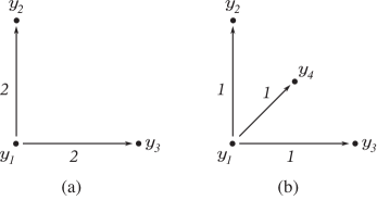
Figure 2: Examples of dynamically equivalent networks (a) and (b).

3 Weakly reversible deficiency one networks

Deficiency analysis [9, 10, 7, 21] forms an integral component of reaction network theory. The dynamics generated by reaction networks with low deficiency has been studied extensively using the Deficiency zero and Deficiency one theorems [2, 8, 9, 10]. In particular, properties like the existence of a unique equilibrium within each stoichiometric compatibility class, local asymptotic stability of the equilibrium owing to the existence of a Lyapunov function have been established. In this paper, we focus on weakly reversible deficiency one reaction networks. Such networks are ubiquitous in applications, and some noteworthy examples are listed below.

Example 3.1 (Edelstein network, [22]).

$$X_{1}\rightleftharpoons 2X_{1},\ X_{1}+X_{2}\rightleftharpoons X_{3}\rightleftharpoons X_{2}$$

This is a weakly reversible reaction network with deficiency $\delta=5-2-2=1$.

Example 3.2 (Symmetry breaking network, [2]).

$$L+2R+P\rightleftharpoons R+Q,\ R+2L+P\rightleftharpoons 3L+Q,\ P\rightleftharpoons 0\rightleftharpoons Q$$

This is a weakly reversible reaction network with the stoichiometric subspace given by:

$$S=\text{span}\{(-1,-1,1,-1)^{\intercal},\ (1,-1,1,-1)^{\intercal},\ (0,-1,0,0)^{\intercal},\ (0,0,-1,0)^{\intercal}\},$$

It is a three-dimensional stoichiometric subspace. The network has deficiency $\delta=7-3-3=1$.

From inequality in Equation (2), deficiency one networks can be classified into the following types :

• $\delta=1=\delta_{1}+\delta_{2}+\cdots+\delta_{\ell}$. We call this a Type I network.

• $\delta=1>\delta_{1}+\delta_{2}+\cdots+\delta_{\ell}$. We call this a Type II network.

Weakly reversible deficiency one networks for which $\delta=1=\delta_{1}+\delta_{2}+\cdots+\delta_{\ell}$ (Type I) fall into the regime of the Deficiency one Theorem, which we state below.

Theorem 3.3 (Deficiency One Theorem, [9, 10]).

Consider a reaction network $G$ consisting of $\ell$ linkage classes $L_{1},L_{2},\cdots,L_{\ell}$. Let us assume that $G$ satisfies the following conditions:

1. $\delta_{i}\leq 1$.

2. $\sum\limits_{i=1}^{\ell}\delta_{i}=\delta$.

3. Each linkage class $L_{i}$ contains exactly one terminal strongly connected component.

If there exists a $\boldsymbol{k}$ for which the mass-action system $(G,\boldsymbol{k})$ possesses a positive equilibrium, then every stoichiometric compatibility class has exactly one positive equilibrium. If $G$ is weakly reversible, then for all values of $\boldsymbol{k}$ the mass-action system $(G,\boldsymbol{k})$ possesses a positive equilibrium.

We also state a theorem [11] that guarantees the existence of positive steady states for weakly reversible systems.

Theorem 3.4 ([11]).

For weakly reversible mass-action systems, there exists a positive steady state within each stoichiometric compatibility class.

Using Theorem 3.4 in conjunction with the Deficiency one Theorem, we conclude that for any weakly reversible deficiency one network of Type I, there exists a unique equilibrium within each stoichiometric compatibility class for all values of the rate constants $\boldsymbol{k}$.

For weakly reversible deficiency one networks of Type II, all linkage classes have deficiency zero and they possess the following geometric property:

Proposition 3.5 ([23, Theorem 9]).

Consider a reaction network $G$. Let $L_{1}$ be a linkage class of $G$. Then $L_{1}$ has deficiency zero if and only if its vertices are affinely independent.

Recall that a set $X$ is a polyhedral cone if $X=\{\boldsymbol{x}:M\boldsymbol{x}\leq\textbf{0}\text{ for some matrix }M\}$. Such a cone is convex. It is pointed, or strongly convex if it does not contain a positive dimensional linear subspace. A pointed polyhedral cone admits a unique (up to scalar multiple) minimal set of generators, and these generating vectors are called extreme vectors [24].

Lemma 3.6.

Consider a mass-action system $(G,\boldsymbol{k})$ with vertices $\{\boldsymbol{y}_{i}\}_{i=1}^{m}$. Let $\boldsymbol{W}$ be the matrix of net reaction vectors of $G$, then we have:

1. $\text{ker}(\boldsymbol{W})\cap\mathbb{R}^{m}_{\geq 0}$ is a pointed polyhedral cone.

2. There exists the minimal set of generators for $\text{ker}(\boldsymbol{W})\cap\mathbb{R}^{m}_{\geq 0}$.

Proof.

1. It is clear that the set $\text{ker}(\boldsymbol{W})\cap\mathbb{R}^{m}_{\geq 0}$ is the solution to $\boldsymbol{W}\nu\geq\textbf{0},-\boldsymbol{W}\nu\geq\textbf{0}$, and $\boldsymbol{I}_{m}\nu\geq\textbf{0}$, and the set is a polyhedral cone. From the definition, a cone contained in the positive orthant $\mathbb{R}^{m}_{\geq 0}$ is always pointed. Therefore, we deduce that $\text{ker}(\boldsymbol{W})\cap\mathbb{R}^{m}_{\geq 0}$ is a pointed polyhedral cone.

2. Since $\text{ker}(\boldsymbol{W})\cap\mathbb{R}^{m}_{\geq 0}$ is a pointed cone, by the Minkowski-Weyl theorem [24, 25], we have

   $$\text{ker}(\boldsymbol{W})\cap\mathbb{R}^{m}_{\geq 0}=\sum\limits_{j=1}^{r}\zeta_{i}\boldsymbol{d}_{i},$$ (15)

   where $\{\boldsymbol{d}_{j}\}_{j=1}^{r}$ is the unique (up to scalar multiple) minimal set of generators of the cone $\text{ker}(\boldsymbol{W})\cap\mathbb{R}^{m}_{\geq 0}$.

∎

Furthermore, using the rank-nullity theorem, we have

$$\text{dim}(\text{ker}(\boldsymbol{W}))=\text{dim}(\text{ker}(\boldsymbol{A}_{\boldsymbol{k}}))+\text{dim}(\text{ker}(\boldsymbol{Y})\cap\text{Im}(\boldsymbol{A}_{\boldsymbol{k}})).$$

Thus the minimal set of generators can be divided into two groups. The next definition illustrates this point.

Definition 3.7 ([26]).

Consider a mass-action system $(G,\boldsymbol{k})$ and let $\boldsymbol{W}$ be the matrix of net reaction vectors of $G$. An extreme vector $\boldsymbol{d}_{i}$ of the cone $\text{ker}(\boldsymbol{W})\cap\mathbb{R}^{m}_{\geq 0}$ is called

1. a cyclic generator, if $\boldsymbol{d}_{i}\in\text{ker}(\boldsymbol{A}_{\boldsymbol{k}})$.

2. a stoichiometric generator, if $\boldsymbol{A}_{\boldsymbol{k}}\boldsymbol{d}_{i}\in\text{ker}(\boldsymbol{Y})\backslash\{\mathbf{0}\}$.

Here we give an example where a reaction network possesses both cyclic and stoichiometric generators.

Example 3.8.

Consider the network shown in Figure 3. This weakly reversible reaction network has two linkage classes, and the deficiency of the entire network is one (i.e. $\delta=1$). Moreover, the net reaction vector matrix follows:

$$\boldsymbol{W}=\begin{pmatrix}1&1&-2&1&-1\\ 1&-1&0&0&0\end{pmatrix},$$ (16)

and

$$\text{ker}(\boldsymbol{W}))=\text{span}\big{\{}(1,1,1,0,0)^{\intercal},\ (1,1,0,-2,0)^{\intercal},\ (1,1,0,0,2)^{\intercal}\big{\}}.$$ (17)

Therefore, we can compute the minimal set of generators of $\text{ker}(\boldsymbol{W})\cap\mathbb{R}^{5}_{\geq 0}$:

1. Cyclic generators:

   $$\boldsymbol{d}_{1}=(1,1,1,0,0)^{\intercal},\ \ \boldsymbol{d}_{2}=(0,0,0,1,1)^{\intercal}.$$ (18)

2. Stoichiometric generators:

   $$\boldsymbol{d}_{3}=(1,1,0,0,2)^{\intercal},\ \ \boldsymbol{d}_{4}=(0,0,1,2,0)^{\intercal}.$$ (19)

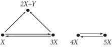
Figure 3: The mass-action system corresponds to Example 3.8, which has both cyclic and stoichiometric generators.

In general, both cyclic and stoichiometric generators can be studied by flux mode analysis. Further, Conradi et al. [26] defined subnetworks generated by stoichiometric generators, and showed that under some conditions if these subnetworks exhibit multistationarity, then so does the original network.

As remarked before, weakly reversible deficiency one realizations of Type I satisfy the conditions of the Deficiency One Theorem. This implies that there exists a unique equilibrium within each stoichiometric compatibility class for all values of the rate constants $\boldsymbol{k}$ of these realizations. Weakly reversible deficiency one realizations of Type II are also important since the subnetworks generated by the stoichiometric generators can help answer questions about multistationarity. It is therefore important to identify and analyze weakly reversible deficiency one realizations.

4 The pointed cone $\text{ker}(\boldsymbol{W})\cap\mathbb{R}^{m}_{\geq 0}$

The goal of this section is to analyze the pointed cone $\text{ker}(\boldsymbol{W})\cap\mathbb{R}^{m}_{\geq 0}$ for weakly reversible deficiency one reaction networks. Specifically, we focus on the extreme vectors of $\text{ker}(\boldsymbol{W})\cap\mathbb{R}^{m}_{\geq 0}$.

Lemma 4.1.

Consider a weakly reversible mass-action system $(G,\boldsymbol{k})$ with vertices $\{\boldsymbol{y}_{i}\}_{i=1}^{m}$. Let $\boldsymbol{W}$ be the matrix of net reaction vectors of $G$, and $\{\boldsymbol{d}_{1},\ldots,\boldsymbol{d}_{r}\}$ be the minimal set of generators of $\text{ker}(\boldsymbol{W})\cap\mathbb{R}^{m}_{\geq 0}$, then

$$\bigcup\limits_{i=1}^{r}\text{supp}(\boldsymbol{d}_{i})=[m].$$ (20)

Proof.

For contradiction, assume there exists $j\in[m]$, such that $j\notin\bigcup\limits_{i=1}^{r}\text{supp}(\boldsymbol{d}_{i})$. Then for any $\boldsymbol{v}=(v_{1},\ldots,v_{m})^{\intercal}\in\text{ker}(\boldsymbol{W})\cap\mathbb{R}^{m}_{\geq 0}$, we obtain that

$$\boldsymbol{v}_{j}=0.$$ (21)

Since $(G,\boldsymbol{k})$ is a weakly reversible mass-action system, by Proposition 2.8 there exists a positive vector in the kernel of the Kirchoff matrix $\boldsymbol{A}_{\boldsymbol{k}}$. Note that weakly reversibility indicates $\boldsymbol{W}=\boldsymbol{Y}\boldsymbol{A}_{\boldsymbol{k}}$. Thus we have

$$\text{ker}(\boldsymbol{A}_{\boldsymbol{k}})\subseteq\text{ker}(\boldsymbol{Y}\boldsymbol{A}_{\boldsymbol{k}})=\text{ker}(\boldsymbol{W}).$$

This implies the existence of a positive vector in $\text{ker}(\boldsymbol{W})\cap\mathbb{R}^{m}_{\geq 0}$, contradicting Equation (21). ∎

Lemma 4.2 ([27]).

Consider a weakly reversible mass-action system $(G,\boldsymbol{k})$ with vertices $\{\boldsymbol{y}_{i}\}_{i=1}^{m}$ and stoichiometric subspace $S$. Let $\boldsymbol{W}$ be the matrix of net reaction vectors of $G$, then

$$\text{Im}(\boldsymbol{W})=S.$$ (22)

The following lemma concerns the dimension of $\text{ker}(\boldsymbol{W})$ in various cases.

Lemma 4.3.

Consider a weakly reversible mass-action system $(G,\boldsymbol{k})$ with vertices $\{\boldsymbol{y}_{i}\}_{i=1}^{m}$ and stoichiometric subspace $S$. Let $\boldsymbol{W}$ be the matrix of net reaction vectors of $G$.

1. If $G$ has deficiency $\delta$ and a single linkage class (i.e. $\ell=1$), we have

   $$\text{dim}(\text{ker}(\boldsymbol{W}))=\delta+1.$$ (23)

   Moreover, if $\delta=0$, then for any $\boldsymbol{z}\in\text{ker}(\boldsymbol{W})\backslash\{\mathbf{0}\}$, $\text{supp}(\boldsymbol{z})=[m]$.

2. If $G$ has deficiency one and $\ell\geq 1$ linkage classes, we have

   $$\text{dim}(\text{ker}(\boldsymbol{W}))=\ell+1.$$ (24)

Proof.

$(a)$ Since $G$ has deficiency $\delta$ and one linkage class, we have

$$\dim(S)=s=m-(\delta+1).$$

By Lemma 4.2, $\text{rank}(\boldsymbol{W})=\dim(\text{Im}(\boldsymbol{W}))=s$. Using the rank-nullity theorem, we obtain

$$\text{dim}(\text{ker}(\boldsymbol{W}))=\delta+1.$$

Furthermore, if $\delta=0$, we deduce that

$$\text{dim}(\text{ker}(\boldsymbol{W}))=1.$$ (25)

As a weakly reversible mass-action system, $(G,\boldsymbol{k})$ possesses a strictly positive steady state $\hat{\boldsymbol{x}}\in\mathbb{R}^{n}_{>0}$ by Theorem 3.4. Using Equation (3), we get

$$\sum\limits_{j\in[m]}{\hat{\boldsymbol{x}}}^{\boldsymbol{y}_{j}}\sum\limits_{\boldsymbol{y}_{j}\to\boldsymbol{y}_{j}^{\prime}\in\mathcal{R}}k_{\boldsymbol{y}_{j}\to\boldsymbol{y}_{j}^{\prime}}(\boldsymbol{y}_{j}^{\prime}-\boldsymbol{y}_{j})=\sum\limits_{j\in[m]}{\hat{\boldsymbol{x}}}^{\boldsymbol{y}_{j}}\boldsymbol{w}_{j}=0.$$ (26)

Note that $({\hat{\boldsymbol{x}}}^{\boldsymbol{y}_{1}},{\hat{\boldsymbol{x}}}^{\boldsymbol{y}_{2}},\ldots,{\hat{\boldsymbol{x}}}^{\boldsymbol{y}_{m}})\in\mathbb{R}^{m}_{>0}$, and it spans $\text{ker}(\boldsymbol{W})$ due to Equation (25).

$(b)$ Since the deficiency of $G$ is one, we get

$$\dim(S)=s=m-\ell-\delta=m-(\ell+1).$$

From Lemma 4.2, we conclude that

$$\text{dim}(\text{ker}(\boldsymbol{W}))=m-\dim(\text{Im}(\boldsymbol{W}))=m-\dim(S)=\ell+1.$$

∎

Here we start with the minimal set of generators of $\text{ker}(\boldsymbol{W})\cap\mathbb{R}^{m}_{\geq 0}$, when weakly reversible mass-action systems contain a single linkage class.

Lemma 4.4.

Consider a weakly reversible mass-action system $(G,\boldsymbol{k})$ that has deficiency $\delta$ and a single linkage class $L=\{\boldsymbol{y}_{1},\ldots,\boldsymbol{y}_{m}\}$. Let $\boldsymbol{W}$ be the matrix of net reaction vectors of $G$, and $\{\boldsymbol{d}_{1},\ldots,\boldsymbol{d}_{r}\}$ be the minimal set of generators of $\text{ker}(\boldsymbol{W})\cap\mathbb{R}^{m}_{\geq 0}$, then

$$r\geq\delta+1.$$ (27)

Moreover, if $\delta=1$, then $r=2$. Assume $\{\boldsymbol{d}_{1},\boldsymbol{d}_{2}\}$ is the minimal set of generators, then

$$\text{supp}(\boldsymbol{d}_{1})\subsetneq[m],\ \ \text{supp}(\boldsymbol{d}_{2})\subsetneq[m],\ \ \text{supp}(\boldsymbol{d}_{1})\cup\text{supp}(\boldsymbol{d}_{2})=[m].$$ (28)

Proof.

Since $G$ has deficiency $\delta$ and one linkage class, from Lemma 4.3.(a) we obtain

$$\text{dim}(\text{ker}(\boldsymbol{W}))=\delta+1.$$

Using Equation (26) in Lemma 4.3, we set $\boldsymbol{d}=(\boldsymbol{x}^{\boldsymbol{y}_{1}},\boldsymbol{x}^{\boldsymbol{y}_{2}},\ldots,\boldsymbol{x}^{\boldsymbol{y}_{m}})$ where $\boldsymbol{x}\in\mathbb{R}^{n}_{>0}$ is a steady state for the system, and obtain $\boldsymbol{d}\in\text{ker}(\boldsymbol{W})\cap\mathbb{R}^{m}_{\geq 0}$. Then there exists a basis of $\text{ker}(\boldsymbol{W})$ that contains $\boldsymbol{d}$ as follows.

$$B=\{\boldsymbol{d},\boldsymbol{e}_{1},\ldots,\boldsymbol{e}_{\delta}\}.$$

Since $\boldsymbol{d}\in\mathbb{R}^{m}_{>0}$, for any weights $\lambda_{1},\ldots,\lambda_{\delta}$, we can always find a sufficiently large $\lambda>0$, such that

$$\sum\limits^{\delta}_{i=1}\lambda_{i}\boldsymbol{e}_{i}+\lambda\boldsymbol{d}\in\mathbb{R}^{m}_{>0}.$$

Thus, we conclude

$$r\geq\text{dim}(\text{ker}(\boldsymbol{W}))=\delta+1.$$

Furthermore, if the system has deficiency one (i.e. $\delta=1$), we derive that

$$\text{dim}(\text{ker}(\boldsymbol{W}))=\delta+1=2,$$

and thus $\text{ker}(\boldsymbol{W})\cap\mathbb{R}^{m}_{\geq 0}$ is a two-dimensional pointed cone. Therefore, the cone $\text{ker}(\boldsymbol{W})\cap\mathbb{R}^{m}_{\geq 0}$ must have two generators, i.e., $r=2$.

Now assume $\{\boldsymbol{d}_{1},\boldsymbol{d}_{2}\}$ is the minimal set of generators of $\text{ker}(\boldsymbol{W})\cap\mathbb{R}^{m}_{\geq 0}$ when the system has deficiency one. Using $\boldsymbol{d}=(\boldsymbol{x}^{\boldsymbol{y}_{1}},\boldsymbol{x}^{\boldsymbol{y}_{2}},\ldots,\boldsymbol{x}^{\boldsymbol{y}_{m}})\in\mathbb{R}^{m}_{>0}$, we derive that

$$\text{supp}(\boldsymbol{d}_{1})\cup\text{supp}(\boldsymbol{d}_{2})=[m].$$

Suppose $\text{supp}(\boldsymbol{d}_{1})=[m]$, thus $\boldsymbol{d}_{1}\in\mathbb{R}^{m}_{>0}$. Then we can find a sufficiently large $\lambda>0$, such that

$$\boldsymbol{v}=\lambda\boldsymbol{d}_{1}-\boldsymbol{d}_{2}\in\text{ker}(\boldsymbol{W})\cap\mathbb{R}^{m}_{>0}.$$

Note that $\boldsymbol{d}_{1}$ and $\boldsymbol{d}_{2}$ are linearly independent, this contradicts with $\{\boldsymbol{d}_{1},\boldsymbol{d}_{2}\}$ being the generating set of $\text{ker}(\boldsymbol{W})\cap\mathbb{R}^{m}_{\geq 0}$. Thus, we derive that $\text{supp}(\boldsymbol{d}_{1})\subsetneq[m]$. Similarly, we can show $\text{supp}(\boldsymbol{d}_{2})\subsetneq[m]$, and conclude (28). ∎

Lemma 4.5.

Consider a weakly reversible mass-action system $(G,\boldsymbol{k})$ with a single linkage class $L=\{\boldsymbol{y}_{1},\ldots,\boldsymbol{y}_{m}\}$, and let $\boldsymbol{W}$ be the matrix of net reaction vectors of $G$. Then there exists a vector $\boldsymbol{d}\in\mathbb{R}^{m}_{\geq 0}$ generating the cone $\text{ker}(\boldsymbol{W})\cap\mathbb{R}^{m}_{\geq 0}$ if and only if the system has deficiency zero.

Proof.

First, suppose the system has deficiency zero. From Equation (26) in Lemma 4.3, we set $\boldsymbol{d}=(\boldsymbol{x}^{\boldsymbol{y}_{1}},\boldsymbol{x}^{\boldsymbol{y}_{2}},\ldots,\boldsymbol{x}^{\boldsymbol{y}_{m}})$ where $\boldsymbol{x}\in\mathbb{R}^{n}_{>0}$ is a steady state for the system $(G,\boldsymbol{k})$, and obtain

$$\text{ker}(\boldsymbol{W})=\text{span}\{\boldsymbol{d}\}.$$

One can check $\boldsymbol{d}\in\mathbb{R}^{m}_{>0}$, and hence $\boldsymbol{d}$ generates $\text{ker}(\boldsymbol{W})\cap\mathbb{R}^{m}_{\geq 0}$.

On the other hand, consider a vector $\boldsymbol{d}$ that generates $\text{ker}(\boldsymbol{W})\cap\mathbb{R}^{m}_{\geq 0}$. Using (27) and deficiency is non-negative, we get that

$$0\leq\delta\leq 1-1=0.$$ (29)

Thus, we conclude the deficiency of the system is zero. ∎

The remark below follows from Lemmas 4.4 and 4.5.

Remark 4.6.

Consider a weakly reversible mass-action system $(G,\boldsymbol{k})$ with a single linkage class $L=\{\boldsymbol{y}_{i}\}_{i=1}^{m}$. Let $\boldsymbol{W}$ be the matrix of net reaction vectors of $G$. Suppose two vectors $\boldsymbol{d}_{1},\boldsymbol{d}_{2}$ form the minimal set of generators of $\text{ker}(\boldsymbol{W})\cap\mathbb{R}^{m}_{\geq 0}$, then $(G,\boldsymbol{k})$ has deficiency one.

Next, we work on the minimal set of generators of $\text{ker}(\boldsymbol{W})\cap\mathbb{R}^{m}_{\geq 0}$ when the weakly reversible deficiency one networks have multiple linkage classes.

Lemma 4.7.

Consider a weakly reversible deficiency one mass-action system $(G,\boldsymbol{k})$ of Type I that has $\ell>1$ linkage classes, denoted by $L_{1},\ldots,L_{\ell}$. Let $\boldsymbol{W}$ be the matrix of net reaction vectors of $G$, and $\{\boldsymbol{W}_{p}\}^{\ell}_{p=1}$ be the matrix of net vectors corresponding to linkage classes $\{L_{p}\}^{\ell}_{p=1}$, then

1. $$\text{dim}(\text{ker}(\boldsymbol{W}_{1}))+\cdots+\text{dim}(\text{ker}(\boldsymbol{W}_{\ell}))=\text{dim}(\text{ker}(\boldsymbol{W}))=\ell+1,$$ (30)

   where

   $$\text{dim}(\text{ker}(\boldsymbol{W}_{i}))=\begin{cases}1,&\text{for }1\leq i\leq\ell-1,\\[5.0pt] 2,&\text{for }i=\ell.\end{cases}$$

   Moreover, for any $1\leq i\leq\ell-1$ and $\boldsymbol{z}\in\text{ker}(\boldsymbol{W}_{i})\backslash\{\mathbf{0}\}$, we have $\text{supp}(\boldsymbol{z})=L_{i}$.

2. There exist $\ell+1$ vectors $\boldsymbol{d}_{1},\ldots,\boldsymbol{d}_{\ell+1}$, which form the minimal set of generators of the cone $\text{ker}(\boldsymbol{W})\cap\mathbb{R}^{m}_{\geq 0}$, such that

   $$\text{supp}(\boldsymbol{d}_{i})=L_{i},\ \text{for }1\leq i\leq\ell-1,$$ (31)

   and

   $$\text{supp}(\boldsymbol{d}_{\ell})\subsetneq L_{\ell},\ \ \text{supp}(\boldsymbol{d}_{\ell+1})\subsetneq L_{\ell},\ \ \text{supp}(\boldsymbol{d}_{\ell})\cup\text{supp}(\boldsymbol{d}_{\ell+1})=L_{\ell}.$$ (32)

Proof.

$(a)$ From the assumption, the system $G$ is of Type I with $\delta_{1}=\cdots=\delta_{\ell-1}=0$ and $\delta_{\ell}=1$. Using Lemma 4.3, we get

$$\text{dim}(\text{ker}(\boldsymbol{W}_{\ell}))=\delta_{\ell}+1=2,\ \ \text{dim}(\text{ker}(\boldsymbol{W}_{i}))=\delta_{i}+1=1,\ \text{for }1\leq i\leq\ell-1.$$

Further, for any $1\leq i\leq\ell-1$ and $\boldsymbol{z}\in\text{ker}(\boldsymbol{W}_{i})\backslash\{\mathbf{0}\}$,

$$\text{supp}(\boldsymbol{z})=L_{i}.$$

Note that $G$ has deficiency one, thus $\text{dim}(\text{ker}(\boldsymbol{W}))=\ell+1$, and we derive (30).

$(b)$ Now we construct the minimal set of generators of $\text{ker}(\boldsymbol{W})\cap\mathbb{R}^{m}_{\geq 0}$, denoted by $\{\boldsymbol{d}_{1},\ldots,\boldsymbol{d}_{r}\}$. It will follow from the construction that $r=\ell+1=\text{dim}(\text{ker}(\boldsymbol{W}))$.

Since $(G,\boldsymbol{k})$ is a weakly reversible mass-action system, it possesses a strictly positive steady state $\hat{\boldsymbol{x}}\in\mathbb{R}^{n}_{>0}$ by Theorem 3.4. Following Equation (26) in Lemma 4.3, we can build $\ell-1$ vectors $\boldsymbol{d}_{1},\ldots,\boldsymbol{d}_{\ell-1}$. We define $\boldsymbol{d}_{1}=(\boldsymbol{d}_{1,1},\ldots,\boldsymbol{d}_{1,m})\in\text{ker}(\boldsymbol{W})\cap\mathbb{R}^{m}_{\geq 0}$, such that

$$\boldsymbol{d}_{1,i}=\begin{cases}\hat{\boldsymbol{x}}^{\boldsymbol{y}_{i}},&\text{for }i\in L_{1},\\ 0,&\text{for }i\notin L_{1}.\end{cases}$$ (33)

It is clear that $\text{supp}(\boldsymbol{d}_{1})=L_{1}$. Analogously, for $i=1,\ldots,\ell-1$, we can define $\boldsymbol{d}_{i}$ corresponding to the linkage classes $L_{i}$ with $\text{supp}(\boldsymbol{d}_{i})=L_{i}$.

Note that $G$ is of Type I and the linkage class $L_{\ell}$ has deficiency one. Let $L_{\ell}=\big{\{}\boldsymbol{y}_{\ell_{i}}\big{\}}^{m_{\ell}}_{i=1}$ with $m_{\ell}=|L_{\ell}|$. From Lemma 4.4, the cone $\text{dim}(\text{ker}(\boldsymbol{W}_{\ell}))\cap\mathbb{R}^{m_{\ell}}_{\geq 0}$ has two generators, denoted by $\{\boldsymbol{g}_{1},\boldsymbol{g}_{2}\}$. Suppose $\boldsymbol{g}_{1}=\big{(}\boldsymbol{g}_{1,i}\big{)}_{i\in L_{\ell}}$ and $\boldsymbol{g}_{2}=\big{(}\boldsymbol{g}_{2,i}\big{)}_{i\in L_{\ell}}$, then we define $\boldsymbol{d}_{\ell}=(\boldsymbol{d}_{\ell,1},\ldots,\boldsymbol{d}_{\ell,m})$, $\boldsymbol{d}_{\ell+1}=(\boldsymbol{d}_{\ell+1,1},\ldots,\boldsymbol{d}_{\ell+1,m})$ as

$$\begin{split}\boldsymbol{d}_{\ell,i}=\begin{cases}\boldsymbol{g}_{1,i},&\text{for }i\in L_{\ell},\\ 0,&\text{for }i\notin L_{\ell}.\end{cases}\ \ \text{and }\ \boldsymbol{d}_{\ell+1,i}=\begin{cases}\boldsymbol{g}_{2,i},&\text{for }i\in L_{\ell},\\ 0,&\text{for }i\notin L_{\ell}.\end{cases}\end{split}$$ (34)

Note that both $\boldsymbol{d}_{\ell},\boldsymbol{d}_{\ell+1}\in\text{ker}(\boldsymbol{W})\cap\mathbb{R}^{m}_{\geq 0}$, and satisfy Equation (32).

We claim that the vectors $\boldsymbol{d}_{1},\ldots,\boldsymbol{d}_{\ell}$ form a set of generators for $\text{ker}(\boldsymbol{W})\cap\mathbb{R}^{m}_{\geq 0}$. From Equations (33) and (34), we deduce that the vectors $\{\boldsymbol{d}_{i}\}^{\ell+1}_{i=1}$ are linearly independent. Together with $\text{dim}(\text{ker}(\boldsymbol{W}))=\ell+1$, we derive that the set $\{\boldsymbol{d}_{1},\ldots,\boldsymbol{d}_{\ell+1}\}$ is a basis for $\text{ker}(\boldsymbol{W})$. Thus, any vector $\boldsymbol{v}\in\text{ker}(\boldsymbol{W})\cap\mathbb{R}^{m}_{\geq 0}$ can be expressed as

$$\boldsymbol{v}=a_{1}\boldsymbol{d}_{1}+a_{2}\boldsymbol{d}_{2}+\cdots+a_{\ell+1}\boldsymbol{d}_{\ell+1}\in\mathbb{R}^{m}_{\geq 0},$$ (35)

where $a_{1},\ldots,a_{\ell+1}\in\mathbb{R}$. So it suffices to prove all $\{a_{i}\}^{\ell+1}_{i=1}$ are non-negative. Recall $\{L_{i}\}^{\ell}_{i=1}$ are linkage classes with $\text{supp}(\boldsymbol{d}_{i})=L_{i}$, and $\text{supp}(\boldsymbol{d}_{\ell})$, $\text{supp}(\boldsymbol{d}_{\ell+1})\subseteq L_{\ell}$, then we obtain

$$a_{i}\geq 0,\ \text{for }i=1,\ldots,\ell-1.$$

Moreover, we set $\hat{\boldsymbol{v}}=a_{\ell}\boldsymbol{g}_{1}+a_{\ell+1}\boldsymbol{g}_{2}$. From $\sum\limits^{\ell}_{i=1}\text{dim}(\text{ker}(\boldsymbol{W}_{i}))=\text{dim}(\text{ker}(\boldsymbol{W}))$, we derive

$$\hat{\boldsymbol{v}}\in\text{ker}(\boldsymbol{W}_{\ell})\cap\mathbb{R}^{m_{\ell}}_{\geq 0}.$$

Since $\boldsymbol{g}_{1},\boldsymbol{g}_{2}$ form the generators of the cone $\text{dim}(\text{ker}(\boldsymbol{W}_{\ell}))\cap\mathbb{R}^{m_{\ell}}_{\geq 0}$, we have

$$a_{\ell}\geq 0,\ \ a_{\ell+1}\geq 0.$$

Therefore, we prove the claim.

Finally, we show $\{\boldsymbol{d}_{1},\boldsymbol{d}_{2},\ldots,\boldsymbol{d}_{\ell+1}\}$ is the minimal set of generators for $\text{ker}(\boldsymbol{W})\cap\mathbb{R}^{m}_{\geq 0}$. Note from Equations (33) and (34), $\boldsymbol{d}_{\ell+1}$ cannot be generated by $\{\boldsymbol{d}_{i}\}^{\ell}_{i=1}$, thus it suffices to show $\{\boldsymbol{d}_{1},\boldsymbol{d}_{2},\ldots,\boldsymbol{d}_{\ell}\}$ are all extreme vectors.

Suppose not, there exists $1\leq j\leq\ell$, such that $\boldsymbol{d}_{j}$ is not an extreme vector. Then we can find two vectors $\gamma,\theta\in\text{ker}(\boldsymbol{W})\cap\mathbb{R}^{m}_{\geq 0}$ and $0<\lambda<1$, such that

$$\lambda\gamma+(1-\lambda)\theta=\boldsymbol{d}_{j},$$ (36)

where $\gamma\neq\nu\theta$ for any constant $\nu$. From Equation (35), we can express $\gamma$ and $\theta$ as the conical combination of $\{\boldsymbol{d}_{1},\boldsymbol{d}_{2},\ldots,\boldsymbol{d}_{\ell+1}\}$ as

$$\gamma=\sum\limits^{\ell+1}_{i=1}\gamma_{i}\boldsymbol{d}_{i}\ \ \text{and }\ \theta=\sum\limits^{\ell+1}_{i=1}\theta_{i}\boldsymbol{d}_{i},$$

where $\gamma_{i},\ \theta_{i}\geq 0$, for $i=1,\ldots,\ell+1$.

If $j\neq\ell$, from $\text{supp}(\boldsymbol{d}_{j})=L_{j}$ and Equation (36), we derive that $\gamma_{i}=\theta_{i}=0$ for $1\leq i\leq\ell+1,i\neq j$. This implies $\gamma=\gamma_{j}d_{j}$ and $\theta=\theta_{j}d_{j}$, which contradicts with $\gamma\neq\nu\theta$.

If $j=\ell$, we deduce that $\gamma_{i}=\theta_{i}=0$ for $1\leq i\leq\ell+1$ such that $i\neq j$ in a similar way. This implies $\gamma=\gamma_{\ell}\boldsymbol{d}_{\ell}$ and $\theta=\theta_{\ell}\boldsymbol{d}_{\ell}$, which also contradicts with $\gamma\neq\nu\theta$. Therefore we conclude that $\{\boldsymbol{d}_{1},\ldots,\boldsymbol{d}_{\ell+1}\}$ is the minimal set of generators of the cone $\text{ker}(\boldsymbol{W})\cap\mathbb{R}^{m}_{\geq 0}$. ∎

Here we illustrate an example where Lemma 4.7 can be verified.

Example 4.8.

Consider a weakly reversible deficiency one mass-action system shown in Figure 4. This reaction network has two linkage classes. One linkage class has deficiency zero, and the other has deficiency one (i.e. $\delta_{1}=0,\ \delta_{2}=1$), and the deficiency of the entire network is one (i.e. $\delta=1$). Therefore, we have

$$1=\delta=\delta_{1}+\delta_{2}.$$ (37)

For all reactions $\boldsymbol{y}\rightarrow\boldsymbol{y}^{\prime}\in E$, we assume $k_{\boldsymbol{y}\rightarrow\boldsymbol{y}^{\prime}}=1$, and get

$$\boldsymbol{W}_{1}=\begin{pmatrix}1&-1\\ 0&0\end{pmatrix},\ \ \boldsymbol{W}_{2}=\begin{pmatrix}0&0&0\\ 1&0&-1\end{pmatrix},\ \ \boldsymbol{W}=\begin{pmatrix}1&-1&0&0&0\\ 0&0&1&0&-1\end{pmatrix}.$$ (38)

So we can derive that

$$\text{ker}(\boldsymbol{W}_{1}))=\text{span}\left\{\begin{pmatrix}1\\ 1\\ \end{pmatrix}\right\},\ \text{ker}(\boldsymbol{W}_{2}))=\text{span}\left\{\begin{pmatrix}0\\ 1\\ 0\\ \end{pmatrix},\ \ \begin{pmatrix}1\\ 0\\ 1\\ \end{pmatrix}\right\},$$ (39)

and

$$\text{ker}(\boldsymbol{W}))=\text{span}\left\{\begin{pmatrix}1\\ 1\\ 0\\ 0\\ 0\\ \end{pmatrix},\ \ \begin{pmatrix}0\\ 0\\ 0\\ 1\\ 0\\ \end{pmatrix},\ \ \begin{pmatrix}0\\ 0\\ 1\\ 0\\ 1\\ \end{pmatrix}\right\}.$$ (40)

For any vector $\boldsymbol{z}_{1}\in\text{ker}(\boldsymbol{W}_{1})\backslash\{\mathbf{0}\}$, we have

$$\text{supp}(\boldsymbol{z}_{1})=L_{1}.$$ (41)

Then, we compute the minimal set of generators of $\text{ker}(\boldsymbol{W})\cap\mathbb{R}^{5}_{\geq 0}$:

$$\boldsymbol{d}_{2}=\begin{pmatrix}1\\ 1\\ 0\\ 0\\ 0\\ \end{pmatrix},\ \ \boldsymbol{d}_{2}=\begin{pmatrix}0\\ 0\\ 0\\ 1\\ 0\\ \end{pmatrix},\ \ \boldsymbol{d}_{3}=\begin{pmatrix}0\\ 0\\ 1\\ 0\\ 1\\ \end{pmatrix}$$ (42)

This shows that the number of extreme vectors: $r=3$, and

$$r=\text{dim}(\text{ker}(\boldsymbol{W}))=\ell+1,$$ (43)

where $\ell=2$. Moreover, for $q=2,3$,

$$\text{supp}(\boldsymbol{d}_{1})=L_{1},\ \ \text{supp}(\boldsymbol{d}_{q})\cap L_{2}\subsetneq L_{2},\ \ \text{supp}(\boldsymbol{d}_{2})\cup\text{supp}(\boldsymbol{d}_{3})=L_{2}.$$ (44)

Therefore, we verify Lemma 4.7.

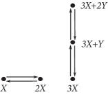
Figure 4: A weakly reversible deficiency one mass-action system of Type I from Example 4.8

Lemma 4.9.

Consider a weakly reversible deficiency one mass-action system $(G,\boldsymbol{k})$ of Type II that has $\ell>1$ linkage classes denoted by $L_{1},\ldots,L_{\ell}$. Let $\boldsymbol{W}$ be the matrix of net reaction vectors of $G$, and $\{\boldsymbol{W}_{p}\}^{\ell}_{p=1}$ be the matrix of net reaction vectors corresponding to linkage classes $\{L_{p}\}^{\ell}_{p=1}$, then

1. $$\text{dim}(\text{ker}(\boldsymbol{W}_{1}))+\cdots+\text{dim}(\text{ker}(\boldsymbol{W}_{\ell}))=\text{dim}(\text{ker}(\boldsymbol{W}))-1=\ell,$$ (45)

   where

   $$\text{dim}(\text{ker}(\boldsymbol{W}_{i}))=1,\ \text{for }1\leq i\leq\ell.$$

   Moreover, for any $1\leq i\leq\ell$ and $\boldsymbol{z}\in\text{ker}(\boldsymbol{W}_{i})\backslash\{\mathbf{0}\}$, we have $\text{supp}(\boldsymbol{z})=L_{i}$.

2. There exist $\ell+2$ vectors $\boldsymbol{d}_{1},\ldots,\boldsymbol{d}_{\ell+2}$, which form the minimal set of generators of the cone $\text{ker}(\boldsymbol{W})\cap\mathbb{R}^{m}_{\geq 0}$, such that for $i=1,\ldots,\ell$,

   $$\text{supp}(\boldsymbol{d}_{i})=L_{i},\ \ \emptyset\neq\text{supp}(\boldsymbol{d}_{\ell+1})\cap L_{i}\subsetneq L_{i},\ \ \emptyset\neq\text{supp}(\boldsymbol{d}_{\ell+2})\cap L_{i}\subsetneq L_{i}.$$ (46)

Proof.

$(a)$ From the assumption, the system $G$ is of Type II with $\delta_{1}=\cdots=\delta_{\ell}=0$. Using Lemma 4.3, we get for $i=1,\ldots,\ell$,

$$\text{dim}(\text{ker}(\boldsymbol{W}_{i}))=\delta_{i}+1=1.$$

Further, for any $1\leq i\leq\ell$ and $\boldsymbol{z}\in\text{ker}(\boldsymbol{W}_{i})\backslash\{\mathbf{0}\}$,

$$\text{supp}(\boldsymbol{z})=L_{i}.$$

Note that $G$ has deficiency one, thus $\text{dim}(\text{ker}(\boldsymbol{W}))=\ell+1$, and we derive (45).

$(b)$ Now we construct the minimal set of generators of $\text{ker}(\boldsymbol{W})\cap\mathbb{R}^{m}_{\geq 0}$, denoted by $\{\boldsymbol{d}_{1},\ldots,\boldsymbol{d}_{r}\}$. It will follow from the construction that $r=\ell+2=\text{dim}(\text{ker}(\boldsymbol{W}))+1$.

Since $(G,\boldsymbol{k})$ is a weakly reversible mass-action system, it possesses a strictly positive steady state $\hat{\boldsymbol{x}}\in\mathbb{R}^{n}_{>0}$ by Theorem 3.4. Following Equation (26) in Lemma 4.3, we can build $\ell$ vectors $\boldsymbol{d}_{1},\ldots,\boldsymbol{d}_{\ell}$. We define $\boldsymbol{d}_{1}=(\boldsymbol{d}_{1,1},\ldots,\boldsymbol{d}_{1,m})\in\text{ker}(\boldsymbol{W})\cap\mathbb{R}^{m}_{\geq 0}$, such that

$$\boldsymbol{d}_{1,i}=\begin{cases}\boldsymbol{x}^{\boldsymbol{y}_{i}},&\text{for }i\in L_{1},\\ 0,&\text{for }i\notin L_{1},\end{cases}$$ (47)

It is clear that $\text{supp}(\boldsymbol{d}_{1})=L_{1}$. Analogously, for $i=1,\ldots,\ell$, we can define $\boldsymbol{d}_{i}$ corresponding to the linkage classes $L_{i}$, with $\text{supp}(\boldsymbol{d}_{i})=L_{i}$.

Now we show that there exists a non-zero vector $\boldsymbol{d}_{\ell+1}\in\text{ker}(\boldsymbol{W})\cap\mathbb{R}^{m}_{\geq 0}$, such that

$$\text{supp}(\boldsymbol{d}_{\ell+1})\cap L_{i}\subsetneq L_{i},\ \text{for }i=1,\ldots,\ell.$$ (48)

From Equation (45), there exists a vector $\tilde{\boldsymbol{d}}\in\text{ker}(\boldsymbol{W})\backslash\{\mathbf{0}\}$, which is linearly independent from $\{\boldsymbol{d}_{i}\}^{\ell}_{i=1}$. Since $\boldsymbol{d}_{i}\in\text{ker}(\boldsymbol{W})\cap\mathbb{R}^{m}_{\geq 0}$ with $\text{supp}(\boldsymbol{d}_{i})=L_{i}$, we set for $i=1,\ldots,\ell$,

$$\alpha_{i}=\max_{k\in L_{i}}\Big{\{}-\frac{\tilde{\boldsymbol{d}}_{k}}{\boldsymbol{d}_{i,k}}\Big{\}}.$$ (49)

Then we define $\boldsymbol{d}_{\ell+1}$ as

$$\boldsymbol{d}_{\ell+1}=\sum\limits^{\ell}_{i=1}\alpha_{i}\boldsymbol{d}_{i}+\tilde{\boldsymbol{d}}.$$ (50)

For any $1\leq j\leq\ell$ and $\theta\in L_{j}$, we obtain that

$$\boldsymbol{d}_{\ell+1,\theta}=\alpha_{j}\boldsymbol{d}_{i,\theta}+\tilde{\boldsymbol{d}}_{\theta}\geq-\frac{\tilde{\boldsymbol{d}}_{\theta}}{\boldsymbol{d}_{i,\theta}}\boldsymbol{d}_{i,\theta}+\tilde{\boldsymbol{d}}_{\theta}=0,$$

and the inequality holds when $\theta=k\in L_{j}$ in Equation (49). Moreover, the linear independence between $\tilde{\boldsymbol{d}}$ and $\{\boldsymbol{d}_{i}\}^{\ell}_{i=1}$ implies that $\boldsymbol{d}_{\ell+1}$ is non-zero. Thus, we show $\boldsymbol{d}_{\ell+1}\in\text{ker}(\boldsymbol{W})\cap\mathbb{R}^{m}_{\geq 0}$, and it satisfies Equation (48).

Furthermore, we claim that there exist at least two linkage classes: $L_{i}$, $L_{j}$ with $1\leq i,j\leq\ell$ and $i\neq j$, such that

$$\text{supp}(\boldsymbol{d}_{\ell+1})\cap L_{i}\neq\emptyset,\ \text{supp}(\boldsymbol{d}_{\ell+1})\cap L_{j}\neq\emptyset.$$ (51)

Suppose not, we assume that only the linkage class $L_{1}$ satisfies $\text{supp}(\boldsymbol{d}_{\ell+1})\cap L_{1}\neq\emptyset$. This implies that

$$\text{supp}(\boldsymbol{d}_{\ell+1})\cap L_{1}\subsetneq L_{1}.$$

Using $\text{dim}(\text{ker}(\boldsymbol{W}_{1}))=1$, we get that $\boldsymbol{d}_{\ell+1}$ must be a scalar multiple of $\boldsymbol{d}_{1}$, contradicting Equation (50).

Next, we construct another non-zero vector $\boldsymbol{d}_{\ell+2}\in\text{ker}(\boldsymbol{W})\cap\mathbb{R}^{m}_{\geq 0}$, such that

$$\text{supp}(\boldsymbol{d}_{\ell+2})\cap L_{i}\subsetneq L_{i},\ \text{for}\ i=1,\ldots,\ell.$$ (52)

Given $\boldsymbol{d}_{1},\ldots,\boldsymbol{d}_{\ell},\boldsymbol{d}_{\ell+1}\in\mathbb{R}^{m}_{\geq 0}$, we set for $i=1,\ldots,\ell$,

$$\beta_{i}=\max_{k\in L_{i}}\Big{\{}\frac{\boldsymbol{d}_{\ell+1,k}}{\boldsymbol{d}_{i,k}}\Big{\}}.$$ (53)

It is clear that $\beta_{i}\geq 0$ for $1\leq i\leq\ell$, then we define $\boldsymbol{d}_{\ell+2}$ as

$$\boldsymbol{d}_{\ell+2}=\sum\limits^{\ell}_{i=1}\beta_{i}\boldsymbol{d}_{i}-\boldsymbol{d}_{\ell+1}.$$ (54)

For any $1\leq j\leq\ell$ and $\theta\in L_{j}$, we get

$$\boldsymbol{d}_{\ell+2,\theta}=\beta_{j}\boldsymbol{d}_{i,\theta}-\boldsymbol{d}_{\ell+1,\theta}\geq\frac{\boldsymbol{d}_{\ell+1,\theta}}{\boldsymbol{d}_{i,\theta}}\boldsymbol{d}_{i,\theta}-\boldsymbol{d}_{\ell+1,\theta}=0$$

The inequality holds when $\theta=k\in L_{j}$ in Equation (53). Moreover, the linear independence between $\boldsymbol{d}_{\ell+1}$ and $\{\boldsymbol{d}_{i}\}^{\ell}_{i=1}$ implies that $\boldsymbol{d}_{\ell+2}$ is non-zero. Thus, we show $\boldsymbol{d}_{\ell+2}\in\text{ker}(\boldsymbol{W})\cap\mathbb{R}^{m}_{\geq 0}$, and it satisfies Equation (52). Similarly as in (51), there also exist at least two linkage classes: $L_{i}$, $L_{j}$ with $1\leq i,j\leq\ell$ and $i\neq j$, such that

$$\text{supp}(\boldsymbol{d}_{\ell+2})\cap L_{i}\neq\emptyset,\ \ \text{supp}(\boldsymbol{d}_{\ell+2})\cap L_{j}\neq\emptyset.$$ (55)

We claim that the vectors $\boldsymbol{d}_{1},\ldots,\boldsymbol{d}_{\ell+2}$ form a set of generators of $\text{ker}(\boldsymbol{W})\cap\mathbb{R}^{m}_{\geq 0}$. Using Equations (47) and (50), we deduce the vectors $\{\boldsymbol{d}_{i}\}^{\ell+1}_{i=1}$ are linearly independent. Together with $\text{dim}(\text{ker}(\boldsymbol{W}))=\ell+1$, we get that the set $\{\boldsymbol{d}_{1},\ldots,\boldsymbol{d}_{\ell+1}\}$ is a basis for $\text{ker}(\boldsymbol{W})$. Thus, any vector $\boldsymbol{v}\in\text{ker}(\boldsymbol{W})\cap\mathbb{R}^{m}_{\geq 0}$ can be expressed as

$$\boldsymbol{v}=a_{1}\boldsymbol{d}_{1}+a_{2}\boldsymbol{d}_{2}+\cdots+a_{\ell+1}\boldsymbol{d}_{\ell+1}\in\mathbb{R}^{m}_{\geq 0},$$ (56)

where $a_{1},\ldots,a_{\ell+1}\in\mathbb{R}$. Recall $\{L_{i}\}^{\ell}_{i=1}$ are linkage classes with $\text{supp}(\boldsymbol{d}_{i})=L_{i}$, for $i=1,\ldots,\ell$, and $\text{supp}(\boldsymbol{d}_{\ell+1})$ in Equation (48), then we obtain

$$a_{i}\geq 0,\ \text{for }i=1,\ldots,\ell.$$

If $a_{\ell+1}\geq 0$, it is clear that $\boldsymbol{v}$ can be expressed as a conical combination of $\{\boldsymbol{d}_{1},\boldsymbol{d}_{2},\ldots,\boldsymbol{d}_{\ell+1}\}$ from Equation (56). Otherwise, if $a_{\ell+1}<0$, we rewrite $\boldsymbol{v}$ as

$$\begin{split}\boldsymbol{v}&=a_{1}\boldsymbol{d}_{1}+\cdots+a_{\ell}\boldsymbol{d}_{\ell}+a_{\ell+1}(\sum\limits^{\ell}_{i=1}\beta_{i}\boldsymbol{d}_{i}-\boldsymbol{d}_{\ell+2})\\ &=a_{1}\boldsymbol{d}_{1}+\cdots+a_{\ell}\boldsymbol{d}_{\ell}+a_{\ell+1}\sum\limits^{\ell}_{i=1}\beta_{i}\boldsymbol{d}_{i}-a_{\ell+1}\boldsymbol{d}_{\ell+2}\\ &=(a_{1}+a_{\ell+1}\beta_{1})\boldsymbol{d}_{1}+\cdots+(a_{\ell}+a_{\ell+1}\beta_{\ell})\boldsymbol{d}_{\ell}-a_{\ell+1}\boldsymbol{d}_{\ell+2}.\end{split}$$ (57)

Using $\boldsymbol{v}\in\text{ker}(\boldsymbol{W})\cap\mathbb{R}^{m}_{\geq 0}$ and Equation (52), we get that for $i=1,\ldots,\ell$,

$$a_{i}+a_{\ell+1}\beta_{i}\geq 0,$$

which implies that $\boldsymbol{v}$ can be generated by $\{\boldsymbol{d}_{1},\ldots,\boldsymbol{d}_{\ell},\boldsymbol{d}_{\ell+2}\}$.

Finally, we show $\{\boldsymbol{d}_{1},\boldsymbol{d}_{2},\ldots,\boldsymbol{d}_{\ell+2}\}$ is the minimal set of generators for $\text{ker}(\boldsymbol{W})\cap\mathbb{R}^{m}_{\geq 0}$. Note that $\boldsymbol{d}_{1},\ldots,\boldsymbol{d}_{\ell+1}$ form a basis for $\text{ker}(\boldsymbol{W})$ and $\boldsymbol{d}_{\ell+2}=\sum\limits^{\ell}_{i=1}\beta_{i}\boldsymbol{d}_{i}-\boldsymbol{d}_{\ell+1}$, thus $\boldsymbol{d}_{\ell+2}$ cannot be generated by $\{\boldsymbol{d}_{i}\}^{\ell+1}_{i=1}$. So it suffices to show $\{\boldsymbol{d}_{1},\boldsymbol{d}_{2},\ldots,\boldsymbol{d}_{\ell+1}\}$ are all extreme vectors.

Suppose not, there exists $1\leq j\leq\ell+1$, such that $\boldsymbol{d}_{j}$ is not an extreme vector. Then we can find two vectors $\gamma,\theta\in\text{ker}(\boldsymbol{W})\cap\mathbb{R}^{m}_{\geq 0}$ and $0<\lambda<1$, such that

$$\lambda\gamma+(1-\lambda)\theta=\boldsymbol{d}_{j},$$ (58)

where $\gamma\neq\nu\theta$ for any constant $\nu$. Then we write $\gamma$ and $\theta$ as the combination of $\{\boldsymbol{d}_{i}\}^{\ell+1}_{i=1}$,

$$\gamma=\sum\limits^{\ell+1}_{i=1}\gamma_{i}\boldsymbol{d}_{i},\ \ \theta=\sum\limits^{\ell+1}_{i=1}\theta_{i}\boldsymbol{d}_{i}.$$

Since $\gamma,\theta\in\mathbb{R}^{m}_{\geq 0}$, we have for $i=1,\ldots,\ell$,

$$\gamma_{i}\geq 0,\ \theta_{i}\geq 0.$$

If $j\neq\ell+1$, from Equation (58), we can derive that $\gamma_{i}=\theta_{i}=0$ when $1\leq i\leq\ell,i\neq j$. Since $\gamma,\theta\in\mathbb{R}^{m}_{\geq 0}$, and $\text{supp}(\boldsymbol{d}_{\ell+1})\cap L_{i}\subsetneq L_{i}$ for $i=1,\ldots,\ell$, we derive $\gamma_{\ell+1}=\theta_{\ell+1}=0$. This implies $\gamma=\gamma_{j}d_{j}$ and $\theta=\theta_{j}d_{j}$, and this contradicts with $\gamma\neq\nu\theta$.

If $j=\ell+1$, in a similar way we can deduce that $\gamma_{i}=\theta_{i}=0$ for $1\leq i\leq\ell$. This implies $\gamma=\gamma_{\ell+1}\boldsymbol{d}_{\ell+1}$ and $\theta=\theta_{\ell+1}\boldsymbol{d}_{\ell+1}$, which also contradicts with $\gamma\neq\nu\theta$. Therefore we conclude that $\{\boldsymbol{d}_{1},\ldots,\boldsymbol{d}_{\ell+2}\}$ is the minimal set of generators of the cone $\text{ker}(\boldsymbol{W})\cap\mathbb{R}^{m}_{\geq 0}$. ∎

We also illustrate an example where Lemma 4.9 can be verified.

Example 4.10.

Consider a weakly reversible deficiency one mass-action system shown in Figure 5. This reaction network has two deficiency zero linkage classes (i.e. $\delta_{1}=\delta_{2}=0$), and the deficiency of the entire network is one (i.e. $\delta=1$). Therefore, we have

$$1=\delta>\delta_{1}+\delta_{2}=0+0.$$ (59)

For all reactions $\boldsymbol{y}\rightarrow\boldsymbol{y}^{\prime}\in E$, we assume $k_{\boldsymbol{y}\rightarrow\boldsymbol{y}^{\prime}}=1$, and get

$$\boldsymbol{W}_{1}=\begin{pmatrix}1&-1\\ 0&0\end{pmatrix},\ \ \boldsymbol{W}_{2}=\begin{pmatrix}1&-1\\ 0&0\end{pmatrix},\ \ \boldsymbol{W}=\begin{pmatrix}1&-1&1&-1\\ 0&0&0&0\end{pmatrix}.$$ (60)

So we can derive that

$$\text{ker}(\boldsymbol{W}_{1}))=\text{ker}(\boldsymbol{W}_{2}))=\text{span}\left\{\begin{pmatrix}1\\ 1\\ \end{pmatrix}\right\},$$ (61)

and

$$\text{ker}(\boldsymbol{W}))=\text{span}\left\{\begin{pmatrix}1\\ 1\\ 0\\ 0\\ \end{pmatrix},\ \ \begin{pmatrix}-1\\ 0\\ 1\\ 0\\ \end{pmatrix},\ \ \begin{pmatrix}1\\ 0\\ 0\\ 1\\ \end{pmatrix}\right\}.$$ (62)

For any vectors $\boldsymbol{z}_{1}\in\text{ker}(\boldsymbol{W}_{1})\backslash\{\mathbf{0}\}$ and $\boldsymbol{z}_{2}\in\text{ker}(\boldsymbol{W}_{2})\backslash\{\mathbf{0}\}$, we have

$$\text{supp}(\boldsymbol{z}_{1})=L_{1},\ \ \text{supp}(\boldsymbol{z}_{2})=L_{2}.$$ (63)

Then, we compute the minimal set of generators of $\text{ker}(\boldsymbol{W})\cap\mathbb{R}^{4}_{\geq 0}$:

$$\boldsymbol{d}_{1}=\begin{pmatrix}1\\ 1\\ 0\\ 0\\ \end{pmatrix},\ \ \boldsymbol{d}_{2}=\begin{pmatrix}0\\ 0\\ 1\\ 1\\ \end{pmatrix},\ \ \boldsymbol{d}_{3}=\begin{pmatrix}0\\ 1\\ 1\\ 0\\ \end{pmatrix},\ \ \boldsymbol{d}_{4}=\begin{pmatrix}1\\ 0\\ 0\\ 1\\ \end{pmatrix}.$$ (64)

This indicates the number of extreme vectors: $r=4$ and

$$r=\text{dim}(\text{ker}(\boldsymbol{W}))+1=\ell+2,$$ (65)

where $\ell=2$. Moreover, for $p=1,2$,

$$\text{supp}(\boldsymbol{d}_{p})=L_{p},\ \ \text{supp}(\boldsymbol{d}_{\ell+1})\cap L_{p}\subsetneq L_{p},\ \ \text{supp}(\boldsymbol{d}_{\ell+2})\cap L_{p}\subsetneq L_{p}.$$ (66)

Therefore, we verify Lemma 4.9.

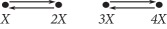
Figure 5: A weakly reversible deficiency one mass-action system of Type II from Example 4.10

To conclude this section, we show that given a mass-action system that admits weakly reversible deficiency one realizations, then these realizations must be of the same type. First, we recall a special result from [28]:

Theorem 4.11 ([28, Theorem 6.3]).

Consider two weakly reversible mass-action systems $(G,\boldsymbol{k})$ and $(G^{\prime},\boldsymbol{k}^{\prime})$ having a deficiency of one and the same number of linkage classes. Let $G$ be of Type I and $G^{\prime}$ be of Type II. Then $(G,\boldsymbol{k})$ and $(G^{\prime},\boldsymbol{k}^{\prime})$ cannot be dynamically equivalent.

After Theorem 4.11, we are ready to prove the more general result as follows:

Theorem 4.12.

Given two weakly reversible deficiency one mass-action systems: $(G,\boldsymbol{k})$ of Type I and $(G^{\prime},\boldsymbol{k}^{\prime})$ of Type II, then $(G,\boldsymbol{k})$ and $(G^{\prime},\boldsymbol{k}^{\prime})$ cannot be dynamically equivalent.

Proof.

For contradiction, assume that the two weakly reversible deficiency one mass-action systems $(G=(V,E),\boldsymbol{k})$ of Type I, and $(G^{\prime}=(V^{\prime},E^{\prime}),\boldsymbol{k}^{\prime})$ of Type II are dynamically equivalent. By Remark 2.11, they have the same set of non-zero net reaction vectors. Using $\text{Im}(\boldsymbol{W})=S$ from Lemma 4.2, we get that $(G,\boldsymbol{k})$ and $(G^{\prime},\boldsymbol{k}^{\prime})$ share the same stoichiometric subspace.

Now we claim that $(G,\boldsymbol{k})$ and $(G^{\prime},\boldsymbol{k}^{\prime})$ have the same number of vertices. For contradiction, suppose there exists a vertex $\boldsymbol{y}\in V^{\prime}$ such that $\boldsymbol{y}\notin V$. Let $\boldsymbol{w}_{\boldsymbol{y}}$ and $\boldsymbol{w}^{\prime}_{\boldsymbol{y}}$ represent the net reaction vectors corresponding to the vertex $\boldsymbol{y}$ in $G$ and $G^{\prime}$. From Remark 2.11, we deduce that

$$\boldsymbol{w}^{\prime}_{\boldsymbol{y}}=\sum\limits_{\boldsymbol{y}\rightarrow\boldsymbol{y}_{j}\in E^{\prime}}k^{\prime}_{\boldsymbol{y}\rightarrow\boldsymbol{y}_{j}}(\boldsymbol{y}_{j}-\boldsymbol{y})=\mathbf{0}.$$ (67)

Since the network $G^{\prime}$ is of Type II, each linkage of $G^{\prime}$ has deficiency zero. By Proposition 3.5, we get that its vertices are affinely independent within each linkage class. This implies that the reaction vectors $\{\boldsymbol{y}_{i}-\boldsymbol{y}\}_{\boldsymbol{y}\rightarrow\boldsymbol{y}_{i}\in E^{\prime}}$ are linearly independent, contradicting Equation (67).

Assume that there exists a vertex $\boldsymbol{y}\in L\subseteq V$ such that $\boldsymbol{y}\notin V^{\prime}$ (where $L$ is some linkage class in $G$). Following the steps in the first part, we have that for any $\boldsymbol{y}^{\prime}\in V^{\prime}$, $\boldsymbol{w}^{\prime}_{\boldsymbol{y}}\neq\mathbf{0}$. This shows that $V^{\prime}\subsetneq V$. Moreover, from $\boldsymbol{y}\notin V^{\prime}$, we get that

$$\boldsymbol{w}_{\boldsymbol{y}}=\mathbf{0}.$$

This implies that the vertices in the linkage class $L$ are not affinely independent. Therefore the deficiency of linkage class $L$ is one. Since $(G,\boldsymbol{k})$ and $(G^{\prime},\boldsymbol{k}^{\prime})$ have the same stoichiometric subspace and deficiency, we deduce that $G$ has at least one more linkage class than $G^{\prime}$. From the Pigeonhole Principle, there exists at least one linkage class in $G^{\prime}$ that is split into different linkage classes in $G$. Let us call this linkage class as $L^{\prime}_{1}\subsetneq V^{\prime}$. Using Lemma 4.3, we have

$$\text{dim}(\text{ker}(\boldsymbol{W}^{\prime}_{1}))\geq 1.$$

where $\boldsymbol{W}^{\prime}_{1}$ is the matrix of net reaction vectors on $L^{\prime}_{1}$. This implies that the stoichiometric subspaces corresponding to the linkage classes in $G$ are not linearly independent, contradicting the fact that $G$ is of Type I.

Since $(G,\boldsymbol{k})$ and $(G^{\prime},\boldsymbol{k}^{\prime})$ have the same stoichiometric subspace, number of vertices, and deficiency we obtain that $(G,\boldsymbol{k})$ and $(G^{\prime},\boldsymbol{k}^{\prime})$ possess the same number of linkage classes. Finally, applying Theorem 4.11, we get that $(G,\boldsymbol{k})$ and $(G^{\prime},\boldsymbol{k}^{\prime})$ cannot be dynamically equivalent, which leads to a contradiction. ∎

The following remark is a direct consequence of Theorem 4.12.

Remark 4.13.

For any mass-action system $(G,\boldsymbol{k})$, it at most has one type of weakly reversible deficiency one realization, i.e. either Type I or Type II.

5 Main results

This section aims to present the main algorithm of this paper, which checks the existence of a weakly reversible deficiency one realization and outputs one if it exists. In this algorithm, the inputs are the matrices of source vertices and net reaction vectors via

$$\boldsymbol{Y}_{s}=(\boldsymbol{y}_{1},\boldsymbol{y}_{2},\ldots,\boldsymbol{y}_{m})\ \ \text{and }\ \boldsymbol{W}=(\boldsymbol{w}_{1},\boldsymbol{w}_{2},\ldots,\boldsymbol{w}_{m})$$

respectively. For the sake of simplicity, we temporarily let $d_{\boldsymbol{W}}=\{\boldsymbol{d}_{1},\boldsymbol{d}_{2},\ldots,\boldsymbol{d}_{r}\}$ denote the minimal set of generators of $\text{ker}(\boldsymbol{W})\cap\mathbb{R}^{m}_{\geq 0}$ in this section.

To build the main algorithm, we need an algorithm to search for a weakly reversible realization with a single linkage class. We use the algorithm in [27] and summarize its main idea as follows.

First, the algorithm in [27] checks whether there exists a reaction network realization that generates the given dynamical system such that all the target vertices are among the source vertices, without imposing the restrictions that $(i)$ the network should be weakly reversible, and $(ii)$ there should be only one linkage class. Next, if such a realization exists, the algorithm greedily searches for a maximal realization (a realization containing the maximum number of reactions) that generates the same dynamical system, while still imposing the restriction that all target vertices are among the source vertices. The algorithm uses the fact that if the initial realization was weakly reversible and consisted of a single linkage class, then the maximal realization found using this procedure preserves weakly reversibility and a single linkage class. Finally, based on this maximal realization, the algorithm constructs a Kirchoff matrix $Q$ and checks whether $\dim(\text{ker}(Q))=1$ and $\text{supp}(\text{ker}(Q))=\{1,2,3,\ldots,m\}$. If both conditions are satisfied, then the maximal realization is weakly reversible and consists of a single linkage class. Otherwise, there is no such realization that generates the given polynomial dynamical system.

For more details on this algorithm and its implementation and complexity, please see [27]. In what follows, we will refer to the algorithm in [27] as Alg-WR^ℓ=1.

5.1 Algorithm for weakly reversible and deficiency one realization

Now we state the main algorithm. The key idea is to find a proper decomposition on $\boldsymbol{W}=\boldsymbol{Y}\boldsymbol{A}_{\boldsymbol{k}}$, which allows a weakly reversible and deficiency one realization. We apply Alg-WR^ℓ=1 to ensure weakly reversibility and the single linkage class condition, and use results in Section 4 to guarantee that the deficiency of the network is one.

   1 (Check the existence of a weakly reversible deficiency one realization)

 

Input: The matrices of source vertices $\boldsymbol{Y}_{s}=(\boldsymbol{y}_{1},\ldots,\boldsymbol{y}_{m})$, and net reaction vectors $\boldsymbol{W}=(\boldsymbol{w}_{1},\ldots,\boldsymbol{w}_{m})$ that generate the dynamical system $\dot{\boldsymbol{x}}=\sum\limits_{i=1}^{m}\boldsymbol{x}^{\boldsymbol{y}_{i}}\boldsymbol{w}_{i}$.

Output: A weakly reversible deficiency one realization if exists or output that it does not exist.

1:Set flag = 0 and $\text{dim}(\text{ker}(\boldsymbol{W}))=\boldsymbol{w}^{*}$;

2:Find the minimal set of generators $d_{\boldsymbol{W}}=\{\boldsymbol{d}_{1},\boldsymbol{d}_{2},\ldots,\boldsymbol{d}_{r}\}$ of the pointed cone $\text{ker}(\boldsymbol{W})\cap\mathbb{R}^{m}_{\geq 0}$.

3:if $r<2$ or $\displaystyle\bigcup_{i=1}^{r}\text{supp}(\boldsymbol{d}_{i})\neq[m]$: then

4:     Exit the main program;

5:else if r = 2 then

6:    Pass $\boldsymbol{Y}_{s},\boldsymbol{W}$ through Alg-WR^ℓ=1

7:    if Alg-WR^ℓ=1 outputs that a weakly reversible realization consisting of a single linkage class does not exist then

8:         Exit the main program;

9:    else

10:         flag=1;

11:         Exit the main program;

12:    end if

13:else

14:    for $i=1,2,\ldots,r-1$ do

15:         for $j=i+1,i+2,\ldots,r$ do

16:             $S_{1}=\{\boldsymbol{d}_{i},\boldsymbol{d}_{j}\}$.

17:             $S_{2}=\boldsymbol{d}_{\boldsymbol{W}}\setminus S_{1}$ and set $S_{2}:=\{\hat{\boldsymbol{d}}_{p}\}^{r-2}_{p=1}$.

18:             if $r=\boldsymbol{w}^{*}$ and the support of $S_{1}$ and every member of $S_{2}$ are disjoint then

19:                 Define linkage classes to be $\{L_{p}\}^{r-1}_{p=1}$, where $L_{p}:=\{\text{supp}(\hat{\boldsymbol{d}}_{p}),\hat{\boldsymbol{d}}_{p}\in S_{2}\}$ for $1\leq p\leq r-2$, and $L_{r-1}:=\{\text{supp}(\boldsymbol{d}_{i})\cup\text{supp}(\boldsymbol{d}_{j})\}$.

20:                 Let $\boldsymbol{Y}_{p}$ denotes the vertices in linkage class $L_{p}$, and $\boldsymbol{W}_{p}$ denotes the matrix of net reaction vectors corresponding to $\boldsymbol{Y}_{p}$.

21:                 for $p=1$ to $r-1$ do

22:                     Pass $\boldsymbol{Y}_{p},\boldsymbol{W}_{p}$ through Alg-WR^ℓ=1

23:                     if Alg-WR^ℓ=1 outputs that a weakly reversible realization consisting of a single linkage class does not exist then

24:                         Go to line 15;

25:                     end if

26:                 end for

27:                  flag=2;

28:                 Exit the main program;

29:             else if $r=\boldsymbol{w}^{*}+1$ and the support of the members of $S_{2}$ partition $[m]$ then

30:                 Define linkage classes to be $\{L_{p}\}^{r-2}_{p=1}$, where $L_{p}:=\{\text{supp}(\hat{\boldsymbol{d}}_{p}),\hat{\boldsymbol{d}}_{p}\in S_{2}\}$ for $1\leq p\leq r-2$.

31:                 Let $\boldsymbol{Y}_{p}$ denotes the vertices in linkage class $L_{p}$, and $\boldsymbol{W}_{p}$ denotes the matrix of net reaction vectors corresponding to $\boldsymbol{Y}_{p}$.

32:                 if $\text{dim}(\text{ker}(\boldsymbol{W}_{1}))=\text{dim}(\text{ker}(\boldsymbol{W}_{2}))=\cdots=\text{dim}(\text{ker}(\boldsymbol{W}_{r-2}))=1$ then

33:                     for $p=1$ to $r-2$ do

34:                         Pass $\boldsymbol{Y}_{p},\boldsymbol{W}_{p}$ through Alg-WR^ℓ=1

35:                         if Alg-WR^ℓ=1 outputs that a weakly reversible realization consisting of a single linkage class does not exist then

36:                             Go to line 15;

37:                         end if

38:                     end for

39:                     flag=3;

40:                     Exit the main program;

41:                 end if

42:             end if

43:         end for

44:    end for

45:end if

46:End of main program

47:if flag = 0 then

48:     Print: No weakly reversible and deficiency one realization exists.

49:else if flag = 1 then

50:     Print: Weakly reversible and deficiency one realization consisting of a single linkage class exists.

51:else if flag = 2 then

52:     Print: Weakly reversible and deficiency one realization of Type I exists.

53:else if flag = 3 then

54:     Print: Weakly reversible and deficiency one realization of Type II exists.

55:end if

 

Figure 6: Algorithm 5.1 for finding a weakly reversible deficiency one realization that generates a given polynomial dynamical system $\dot{\boldsymbol{x}}=\sum\limits_{i=1}^{m}\boldsymbol{x}^{\boldsymbol{y}_{i}}\boldsymbol{w}_{i}$.

Now we show the correctness of Algorithm 5.1 via the following two lemmas.

Lemma 5.1.

Suppose Algorithm 5.1 exits with a positive flag value, then there exists a weakly reversible deficiency one realization of the dynamical system $\dot{\boldsymbol{x}}=\sum\limits_{i=1}^{m}\boldsymbol{x}^{\boldsymbol{y}_{i}}\boldsymbol{w}_{i}$. Moreover, we have

1. If flag = 1, the system admits a weakly reversible deficiency one realization consisting of a single linkage class.

2. If flag = 2, the system admits a weakly reversible deficiency one realization of Type I.

3. If flag = 3, the system admits a weakly reversible deficiency one realization of Type II.

Proof.

$(a)$ From flag $=1$, we obtain that $r=2$ with $\text{supp}(\boldsymbol{d}_{1})\cup\text{supp}(\boldsymbol{d}_{2})=[m]$. Moreover, the input matrices $\boldsymbol{Y}_{s}$ and $\boldsymbol{W}$ pass through Alg-WR^ℓ=1.

Then there exists a weakly reversible realization with a single linkage class that generates the dynamical system $\dot{\boldsymbol{x}}=\sum\limits_{i=1}^{m}\boldsymbol{x}^{\boldsymbol{y}_{i}}\boldsymbol{w}_{i}$. Using Remark 4.6, we conclude its deficiency is one.

$(b)$ From flag $=2$, we get $r=\text{dim}(\text{ker}(\boldsymbol{W}))>2$, and $r-1$ linkage classes $\{L_{1},\ldots,L_{r-1}\}$ as follows. There exists some $1\leq i<j\leq r$,

$$S_{1}=\{\boldsymbol{d}_{i},\boldsymbol{d}_{j}\}\ \ \text{and }\ S_{2}=d_{\boldsymbol{W}}\setminus S_{1}.$$

For the simplicity of notations, we rename $r-2$ vectors in $S_{2}$ as $S_{2}:=\{\hat{\boldsymbol{d}}_{p}\}^{r-2}_{p=1}$ and set

$$\begin{split}&L_{p}=\{\text{supp}(\hat{\boldsymbol{d}}_{p}):\ \hat{\boldsymbol{d}}_{p}\in S_{2}\},\ \text{for}\ 1\leq p\leq r-2,\\ &L_{r-1}=\{\text{supp}(\boldsymbol{d}_{i})\cup\text{supp}(\boldsymbol{d}_{j})\},\end{split}$$

with $\{L_{1},L_{2},\ldots,L_{r-1}\}$ partition $[m]$.

Moreover, for any $1\leq q\leq r-1$, the matrices of source vertices and net reaction vectors $\boldsymbol{Y}_{q},\boldsymbol{W}_{q}$ related to the linkage class $L_{q}$ pass through Alg-WR^ℓ=1. Thus each linkage class $L_{q}$ admits a weakly reversible realization. Together with $\{L_{q}\}^{r-1}_{q=1}$ have disjoint supports in $[m]$, we have

$$\begin{split}&\text{ker}(\boldsymbol{W}_{p})=\{\text{span}(\hat{\boldsymbol{d}}_{p})\},\ \text{for}\ 1\leq p\leq r-2,\\ &\text{ker}(\boldsymbol{W}_{r-1})=\text{span}\{\boldsymbol{d}_{i},\boldsymbol{d}_{j}\}.\end{split}$$ (68)

Using Lemma 4.5 and Remark 4.6 on the realization under Alg-WR^ℓ=1, we get

$$\delta_{1}=\cdots=\delta_{r-1}=0\ \ \text{and }\ \delta_{r-1}=1,$$ (69)

where $\delta_{q}$ represents the deficiency of linkage class $L_{q}$.

Now we compute the deficiency of the whole realization $\delta$. From (LABEL:flag=2_ker_estimate), we obtain

$$\text{dim}(\text{ker}(\boldsymbol{W}_{1})+\text{dim}(\text{ker}(\boldsymbol{W}_{2})+\cdots+\text{dim}(\text{ker}(\boldsymbol{W}_{r-1})=r=\text{dim}(\text{ker}(\boldsymbol{W}).$$ (70)

Applying Lemma 4.2 and Lemma 4.3 on Equation (70), we deduce for $p=1,\ldots,r-1$,

$$\text{dim}(\text{ker}(\boldsymbol{W}_{q}))=1+\delta_{q}=|L_{q}|-s_{q}\ \ \text{and }\ \sum\limits_{q=1}^{r-1}s_{q}=s,$$

where $s_{q}$ and $s$ represent the stoichiometric subspace for linkage class $L_{q}$ and whole network respectively. Then we do the summation from $q=1$ to $r-1$, and get

$$\sum\limits_{q=1}^{r-1}(|L_{q}|-s_{q})=m-s=(r-1)+\sum\limits_{q=1}^{r-1}\delta_{q}.$$

From Equation (69), we conclude that

$$\delta=m-s-(r-1)=\sum\limits_{q=1}^{r-1}\delta_{q}=1,$$

and the system admits a weakly reversible deficiency one realization of Type I.

$(c)$ From flag $=3$, we get $r=\text{dim}(\text{ker}(\boldsymbol{W}))+1>2$, and $r-2$ linkage classes $\{L_{1},\ldots,L_{r-2}\}$ as follows. There exists some $1\leq i<j\leq r$,

$$S_{1}=\{\boldsymbol{d}_{i},\boldsymbol{d}_{j}\}\ \ \text{and }\ S_{2}=d_{\boldsymbol{W}}\setminus S_{1},$$

Similarly, we rename $r-2$ vectors in $S_{2}$ as $S_{2}:=\{\hat{\boldsymbol{d}}_{p}\}^{r-2}_{p=1}$ and set

$$L_{p}=\{\text{supp}(\hat{\boldsymbol{d}}_{p}):\ \hat{\boldsymbol{d}}_{p}\in S_{2}\},\ \text{for}\ 1\leq p\leq r-2,$$

with $\{L_{1},L_{2},\ldots,L_{r-2}\}$ partition $[m]$.

Moreover, for any $1\leq p\leq r-2$, the matrices of source vertices and net reaction vectors $\boldsymbol{Y}_{p},\boldsymbol{W}_{p}$ related to the linkage class $L_{p}$ pass through Alg-WR^ℓ=1. Thus each linkage class $L_{q}$ admits a weakly reversible realization with $\text{dim}(\text{ker}(\boldsymbol{W}_{p}))=1$. Applying that $\{L_{p}\}^{r-2}_{p=1}$ partition $[m]$, we have

$$\text{ker}(\boldsymbol{W}_{p})=\{\text{span}(\hat{\boldsymbol{d}}_{p}):\hat{\boldsymbol{d}}_{p}\in S_{2}\},\ \text{for}\ 1\leq p\leq r-2.$$ (71)

Using Lemma 4.5 on the realization under Alg-WR^ℓ=1, we get

$$\delta_{1}=\cdots=\delta_{r-2}=0,$$ (72)

where $\delta_{p}$ represents the deficiency of linkage class $L_{p}$.

Now we compute the deficiency of the whole realization $\delta$. From (71), we obtain

$$\text{dim}(\text{ker}(\boldsymbol{W}_{1})+\text{dim}(\text{ker}(\boldsymbol{W}_{2})+\cdots+\text{dim}(\text{ker}(\boldsymbol{W}_{r-2})=r-2=\text{dim}(\text{ker}(\boldsymbol{W})-1.$$ (73)

Applying Lemma 4.2 and Lemma 4.3 on Equation (73), we deduce for $p=1,\ldots,r-2$,

$$\text{dim}(\text{ker}(\boldsymbol{W}_{p}))=1+\delta_{p}=|L_{p}|-s_{p}\ \ \text{and }\ \sum\limits_{p=1}^{r-2}s_{p}=s+1,$$

where $s_{p}$ and $s$ represent the stoichiometric subspace for linkage class $L_{p}$ and whole network respectively. Summing from $p=1$ to $r-2$, we get

$$\sum\limits_{p=1}^{r-1}(|L_{p}|-s_{p})=m-(s+1)=(r-2)+\sum\limits_{q=1}^{r-1}\delta_{q}.$$

From Equation (72), we conclude that

$$\delta=m-s-(r-2)=\sum\limits_{q=1}^{r-1}\delta_{q}+1=1,$$

and the system admits a weakly reversible deficiency one realization of Type II. ∎

Lemma 5.2.

Suppose the dynamical system $\dot{\boldsymbol{x}}=\displaystyle\sum_{i=1}^{m}\boldsymbol{x}^{\boldsymbol{y}_{i}}\boldsymbol{w}_{i}$ admits a weakly reversible deficiency one realization, then Algorithm 5.1 must set the flag value to be either $1,2$ or $3$.

Proof.

Note that every weakly reversible deficiency one network belongs to the following:

1. Weakly reversible deficiency one realization consisting of a single linkage class.

2. Weakly reversible deficiency one realization of Type I, with two or more linkage classes.

3. Weakly reversible deficiency one realization of Type II.

Therefore, we split our proof into the above three cases.

Case 1: Suppose the system admits a weakly reversible deficiency one realization consisting of a single linkage class. From Lemma 4.4, we obtain that $r=2$ and the input $\boldsymbol{Y}$ and $\boldsymbol{W}$ pass through Alg-WR^ℓ=1 from the weakly reversibility. Therefore, Algorithm 5.1 will exit with flag $=1$.

Case 2: Suppose the system admits a weakly reversible deficiency one realization of Type I with $\ell>1$ linkage classes, denoted by $L_{1},L_{2},\ldots,L_{\ell}$. From Lemma 4.7, we have

$$\text{dim}(\text{ker}(\boldsymbol{W}_{\ell}))=2\ \ \text{and }\ \text{dim}(\text{ker}(\boldsymbol{W}_{p}))=1,\ \text{for}\ 1\leq p\leq\ell-1,$$

and

$$\text{dim}(\text{ker}(\boldsymbol{W}))=\text{dim}(\text{ker}(\boldsymbol{W}_{1}))+\cdots+\text{dim}(\text{ker}(\boldsymbol{W}_{\ell}))=\ell+1=r.$$

Moreover, there exist $\ell+1$ vectors $\boldsymbol{d}_{1},\ldots,\boldsymbol{d}_{\ell+1}$ forming the minimal set of generators of $\text{ker}(\boldsymbol{W})\cap\mathbb{R}^{m}_{\geq 0}$, such that for $p=1,\ldots,\ell-1$,

$$\text{supp}(\boldsymbol{d}_{p})=L_{p},$$

and

$$\text{supp}(\boldsymbol{d}_{\ell})\subsetneq L_{\ell},\ \ \text{supp}(\boldsymbol{d}_{\ell+1})\subsetneq L_{\ell},\ \ \text{supp}(\boldsymbol{d}_{\ell})\cup\text{supp}(\boldsymbol{d}_{\ell+1})=L_{\ell}.$$

Thus, when $i=\ell$ and $j=\ell+1$, (i.e. $\boldsymbol{d}_{i}=\boldsymbol{d}_{\ell}$ and $\boldsymbol{d}_{j}=\boldsymbol{d}_{\ell+1}$), Algorithm 5.1 will exit with flag $=2$.

Case 3: Suppose the system admits a weakly reversible deficiency one realization of Type II with $\ell>1$ linkage classes, denoted by $L_{1},L_{2},\ldots,L_{\ell}$. From Lemma 4.9, we have

$$\text{dim}(\text{ker}(\boldsymbol{W}_{p}))=1,\ \text{for}\ 1\leq p\leq\ell,$$

and

$$\text{dim}(\text{ker}(\boldsymbol{W}))-1=\text{dim}(\text{ker}(\boldsymbol{W}_{1}))+\cdots+\text{dim}(\text{ker}(\boldsymbol{W}_{\ell}))=\ell=r-2.$$

Moreover, there exist $\ell+2$ vectors $\boldsymbol{d}_{1},\ldots,\boldsymbol{d}_{\ell+2}$ forming the minimal set of generators of $\text{ker}(\boldsymbol{W})\cap\mathbb{R}^{m}_{\geq 0}$, such that for $p=1,\ldots,\ell$,

$$\text{supp}(\boldsymbol{d}_{p})=L_{p},\ \ \text{supp}(\boldsymbol{d}_{\ell+1})\cap L_{p}\subsetneq L_{p},\ \ \text{supp}(\boldsymbol{d}_{\ell+2})\cap L_{p}\subsetneq L_{p}.$$

Again when we pick $i=\ell$ and $j=\ell+1$, Algorithm 5.1 will exit with flag $=3$.

Lastly, we show every mass-action system admitting a weakly reversible deficiency one realization has a unique flag value after applying Algorithm 5.1. Following Remark 4.13, we deduce that if flag $=3$ after passing the same mass-action system through the algorithm, the flag value cannot equal $1$ or $2$. From Lemma 4.5 and Lemma 4.7, we have $r=2$ if flag $=1$, and $r=\ell+1>2$ if flag $=2$. Thus, it is also impossible that the flag equals both $1$ and $2$ on the same mass-action system. Therefore, we show the uniqueness and prove this lemma. ∎

The following remark is a direct consequence of Lemma 5.2.

Remark 5.3.

If Algorithm 5.1 sets the value of flag to 0, then $\dot{\boldsymbol{x}}=\sum\limits_{i=1}^{m}\boldsymbol{x}^{\boldsymbol{y}_{i}}\boldsymbol{w}_{i}$ does not admit a weakly reversible deficiency one realization.

Example 5.4.

Consider the system of differential equations

$$\begin{split}\dot{x}&=-x+x^{2},\\ \dot{y}&=x^{3}-x^{3}y^{2}.\end{split}$$ (74)

We have $n=2$ for the two state variables, and $m=5$ for the five distinct monomials. The matrices of source vertices and net direction vectors are

$$\boldsymbol{Y}_{s}=\begin{pmatrix}1&2&3&3&3\\ 0&0&0&1&2\end{pmatrix},\ \text{and }\ \boldsymbol{W}=\begin{pmatrix}1&-1&0&0&0\\ 0&0&1&0&-1\end{pmatrix}.$$ (75)

respectively, which are inputs to Algorithm 5.1.

Then, we can compute that $\text{dim}(\text{ker}(\boldsymbol{W}))=3$, and extreme vectors of $\text{ker}(\boldsymbol{W})\cap\mathbb{R}^{m}_{\geq 0}$ is given by

$$\boldsymbol{d}_{1}=\begin{pmatrix}1\\ 1\\ 0\\ 0\\ 0\\ \end{pmatrix},\ \ \boldsymbol{d}_{2}=\begin{pmatrix}0\\ 0\\ 0\\ 1\\ 0\\ \end{pmatrix},\ \ \boldsymbol{d}_{3}=\begin{pmatrix}0\\ 0\\ 1\\ 0\\ 1\\ \end{pmatrix}.$$

This shows that $r=3$, and the algorithm enters line 13.

Next, when we pick $i=2$, $S_{1}=\{\boldsymbol{d}_{2},\boldsymbol{d}_{3}\}$ and $S_{2}=\{\boldsymbol{d}_{1}\}$. Note that $r=\text{dim}(\text{ker}(\boldsymbol{W}))=3$, and the support of $S_{1}$ and every member of $S_{2}$ are disjoint, the algorithm defines candidate linkage classes are follows:

$$L_{1}=\{\text{supp}(\boldsymbol{d}_{1})\}=\{1,2\},\ \ L_{2}=\{\text{supp}(\boldsymbol{d}_{2})\cup\text{supp}(\boldsymbol{d}_{3})\}=\{3,4,5\}.$$

Following the candidate linkage classes $L_{1},L_{2}$, we derive the corresponding matrices of source vertices and net direction vectors:

$$\begin{split}&\boldsymbol{Y}_{1}=\begin{pmatrix}1&2\\ 0&0\end{pmatrix},\ \ \boldsymbol{W}_{1}=\begin{pmatrix}1&-1\\ 0&0\end{pmatrix},\ \text{and }\ \boldsymbol{Y}_{2}=\begin{pmatrix}3&3&3\\ 0&1&2\end{pmatrix},\ \ \boldsymbol{W}_{2}=\begin{pmatrix}0&0&0\\ 1&0&-1\end{pmatrix}.\end{split}$$

After that, we pass two pairs $(\boldsymbol{Y}_{1},\boldsymbol{W}_{1})$ and $(\boldsymbol{Y}_{2},\boldsymbol{W}_{2})$ through Alg-WR^ℓ=1. Both pairs pass successfully through Alg-WR^ℓ=1, i.e., a weakly reversible single linkage class exists for both arrangements. Finally, the algorithm sets flag $=2$ on line 27, and exits. Therefore, (74) admits a weakly reversible deficiency one realization of Type I, whose E-graph is shown in Figure 7.

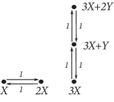
Figure 7: A weakly reversible deficiency one mass-action system from Example 5.4

Example 5.5.

Consider the system of differential equations

$$\begin{split}\dot{x}&=-x+x^{2},\\ \dot{y}&=0.\end{split}$$ (76)

We have $n=2$ for the two state variables, and $m=2$ for the two distinct monomials. The matrices of source vertices and net direction vectors are

$$\boldsymbol{Y}_{s}=\begin{pmatrix}1&2\\ 0&0\end{pmatrix},\ \text{and }\ \boldsymbol{W}=\begin{pmatrix}-1&1\\ 0&0\end{pmatrix}.$$ (77)

respectively, which are inputs to Algorithm 5.1.

Then, we compute that $\text{dim}(\text{ker}(\boldsymbol{W}))=1$, and the extreme vector of $\text{ker}(\boldsymbol{W})\cap\mathbb{R}^{2}_{\geq 0}$ is

$$\boldsymbol{d}_{1}=\begin{pmatrix}1\\ 1\end{pmatrix}.$$

This shows that $r=1$, then the algorithm satisfies the condition on line 4 and exits the program with initial flag $=0$. Therefore, there doesn’t exist any weakly reversible deficiency one realization for this system.

5.2 Implementation of Algorithm 5.1

In this section, we discuss how to implement Algorithm 5.1. The algorithm is designed to find a weakly reversible deficiency one realization that generates the dynamical system $\dot{\boldsymbol{x}}=\sum\limits_{i=1}^{m}\boldsymbol{x}^{\boldsymbol{y}_{i}}\boldsymbol{w}_{i}$, and it has three key steps:

1. Compute $\dim(\ker(\boldsymbol{W}))$ and $\dim(\ker(\boldsymbol{W}_{i}))$.

2. Find the extreme vectors of the cone $\text{ker}(\boldsymbol{W})\cap\mathbb{R}^{m}_{\geq 0}$.

3. Pass pairs of the matrices $\boldsymbol{Y}_{s},\boldsymbol{W}$ or $\boldsymbol{Y}_{i},\boldsymbol{W}_{i}$ through Alg-WR^ℓ=1.

In Step 1, the implementation needs a rank-revealing factorization; we need to find a basis of $\boldsymbol{W}$ or $\boldsymbol{W}_{i}$, and then we can check the number of vectors in this basis. This is equivalent to solving a linear programming problem.

In Step 2, we note that by the Minkowski-Weyl theorem [24, 25], there exists two representations of a polyhedral cone $C$ given by:

1. H-representation: There exists a matrix $A$, such that the cone $C$ can be written as

   $$C=\{Ax\leq 0\}.$$

2. V-representation: The cone $C$ has the minimal set of generators $\{d_{i}\}$, such that

   $$C=\displaystyle\sum_{i=1}^{r}\lambda_{i}d_{i},$$

   where $\lambda_{i}\geq 0$.

To find the extreme vectors of the cone $\text{ker}(\boldsymbol{W})\cap\mathbb{R}^{m}_{\geq 0}$, we need a way to convert from the H-representation to the V-representation. There are two popular ways of performing this conversion:

1. Double description method: This is an example of an incremental method, where the conversion from H-representation to V-representation is performed assuming that the solution to a smaller problem is already known [29]. In particular, let $C(A):=\{Ax\leq 0\}$. Let $J$ be a subset of the row indices of $A$. We will denote by $A_{J}$ the submatrix of $A$ obtained by selecting the $J$ rows of $A$. Let us assume that we have found the minimal set of generators for the cone $C(A_{J})$. We will denote by $E$ the generating matrix whose columns are the extreme vectors of $C(A_{J})$. The double description algorithm selects an index $h$ that is not present in $J$ and constructs the generating matrix $E^{\prime}$ that corresponds to the $A_{J+h}$. This is repeated for several iterations until the generating matrix for $C(A)$ is found. This algorithm is useful in cases where the inputs are degenerate and the dimension of the cone is small.

2. Pivoting methods: In this method, the extreme vectors of the cone are found by the reverse search technique, where the simplex algorithm (that uses pivots iteratively) is run in reverse for the linear programming problem $Ax\leq 0$. The reverse search method determines the extreme vectors of the cone by building a tree in a depth-first-search fashion. This method was developed by Avis and Fukuda [30]. It is particularly useful for non-degenerate inputs where it runs in time polynomial of the input size.

In Step 3, we apply Alg-WR^ℓ=1, and this step can be done by solving a sequence of linear programming problems. More details can be found in section 4.4 in [27].

6 Discussion

Weakly reversible deficiency one networks are ubiquitous in biochemistry, and are known to have the capacity to exhibit sophisticated dynamics. Some notable examples include the Edelstein network, as in Example 3.1. To better understand their dynamics, we divide them into two categories: (i) Type I networks, where all linkage classes have deficiency zero except one linkage class having deficiency one, and (ii) Type II networks, where all linkage classes have deficiency zero. The crucial quantity in the analysis of such networks is the pointed cone $\text{ker}(\boldsymbol{W})\cap\mathbb{R}^{m}_{\geq 0}$, where $\boldsymbol{W}$ is the matrix formed by the net reaction vectors. In particular, the extreme vectors of this cone can be divided into two classes: cyclic generators and stoichiometric generators. Networks of Type I possess only cyclic generators and satisfy the conditions of the Deficiency One Theorem. Consequently, for Type I networks, there exists a unique steady state within every stoichiometric compatibility class. For Type II networks, the set of stoichiometric generators is not empty. The stoichiometric generators define subnetworks, such that if these subnetworks possess multiple steady states, then the original network also allows multiple steady states [26].

In addition, we show that networks of different types cannot be dynamically equivalent. Theorem 4.12 establishes this fact, and this implies that any mass-action system, at most, has one type of weakly reversible deficiency one realization, either Type I or Type II. In Section 4 we analyze in depth the extreme vectors of the cone $\text{ker}(\boldsymbol{W})\cap\mathbb{R}^{m}_{\geq 0}$ for weakly reversible deficiency one networks. In particular, we show that for Type I networks with $\ell$ linkage classes, there exist $\ell+1$ generators, while for Type II networks with $\ell$ linkage classes, there exist $\ell+2$ generators. Lemmas 4.7 and 4.9 establish these facts.

In Section 5 we describe our main result: the construction and the proof of correctness of Algorithm 5.1. This algorithm takes as input a matrix of source vertices and the corresponding matrix of net reaction vectors. Algorithm 5.1 uses Alg-WR^ℓ=1 as a subroutine and determines whether or not there exists a weakly reversible deficiency one realization for this input. It is interesting to put this algorithm in the context of existing algorithms in the literature. There has been seminal work in this direction [31, 32, 33, 34, 35, 36, 37] based mostly on optimization methods that rely on mixed integer linear programming to determine the existence of realizations of a certain type. The algorithm in this paper uses a novel and straightforward geometric approach by focusing on the extreme vectors of the cone $\text{ker}(\boldsymbol{W})\cap\mathbb{R}^{m}_{\geq 0}$, instead of posing it as a constrained optimization problem. Algorithm 5.1 uses Alg-WR^ℓ=1 and the properties of the extreme vectors of the cone $\text{ker}(\boldsymbol{W})\cap\mathbb{R}^{m}_{\geq 0}$ to determine the existence of weakly reversible deficiency one realizations. This geometric approach in both algorithms allows for a fully self-contained mathematical analysis of the correctness of these algorithms.

This work opens up interesting new avenues for future research. In particular, the relationship between the minimal set of generators of the cone $\text{ker}(\boldsymbol{W})\cap\mathbb{R}^{m}_{\geq 0}$ and the deficiency of the network can be explored in greater depth. One could also explore the existence of mutually exclusive types of weakly reversible realizations for networks of higher deficiency. Another possible direction would be to explore the geometry of this minimal set of generators for weakly reversible networks of higher deficiency.

References

• [1] E. Voit, H. Martens, and S. Omholt. 150 years of the mass action law. PLOS Comput. Biol., 11(1):e1004012, 2015.
• [2] M. Feinberg. Foundations of chemical reaction network theory. Springer, 2019.
• [3] J. Gunawardena. Chemical reaction network theory for in-silico biologists. Notes available for download at http://vcp. med. harvard. edu/papers/crnt. pdf, 2003.
• [4] P. Yu and G. Craciun. Mathematical Analysis of Chemical Reaction Systems. Isr. J. Chem., 58(6-7):733–741, 2018.
• [5] G. Craciun and C. Pantea. Identifiability of chemical reaction networks. J. Math. Chem., 44(1):244–259, 2008.
• [6] F. Horn and R. Jackson. General mass action kinetics. Arch. Ration. Mech. Anal., 47(2):81–116, 1972.
• [7] F. Horn. Necessary and sufficient conditions for complex balancing in chemical kinetics. Arch. Ration. Mech. Anal., 49(3):172–186, 1972.
• [8] M. Feinberg. Chemical oscillations, multiple equilibria, and reaction network structure. In Dynamics and modelling of reactive systems, pages 59–130. Elsevier, 1980.
• [9] M. Feinberg. Chemical reaction network structure and the stability of complex isothermal reactors - I. the deficiency zero and deficiency one theorems. Chem. Eng. Sci., 42(10):2229–2268, 1987.
• [10] M. Feinberg. The existence and uniqueness of steady states for a class of chemical reaction networks. Arch. Ration. Mech. Anal., 132(4):311–370, 1995.
• [11] B. Boros. Existence of positive steady states for weakly reversible mass-action systems. SIAM J. Math. Anal., 51(1):435–449, 2019.
• [12] M. Gopalkrishnan, E. Miller, and A. Shiu. A geometric approach to the global attractor conjecture. SIAM J. Appl. Dyn. Syst., 13(2):758–797, 2014.
• [13] D Anderson. A proof of the global attractor conjecture in the single linkage class case. SIAM J. Appl. Math., 71(4):1487–1508, 2011.
• [14] G. Craciun, F. Nazarov, and C. Pantea. Persistence and permanence of mass-action and power-law dynamical systems. SIAM J. Appl. Math., 73(1):305–329, 2013.
• [15] B. Boros and J. Hofbauer. Permanence of weakly reversible mass-action systems with a single linkage class. SIAM J. Appl. Dyn. Syst., 19(1):352–365, 2020.
• [16] G. Craciun, J. Jin, and P. Yu. An algorithm for weakly reversible deficiency zero realizations of polynomial dynamical systems. arXiv preprint arXiv:2205.14267, 2022.
• [17] C. Guldberg and P. Waage. Studies Concerning Affinity. CM Forhandlinger: Videnskabs-Selskabet I Christiana, 35(1864):1864, 1864.
• [18] M. Feinberg. Lectures on chemical reaction networks. Notes of lectures given at the Mathematics Research Center, University of Wisconsin, page 49, 1979.
• [19] L. Adleman, M. Gopalkrishnan, M. Huang, P. Moisset, and D. Reishus. On the mathematics of the law of mass action. In A Systems Theoretic Approach to Systems and Synthetic Biology I: Models and System Characterizations, pages 3–46. Springer, 2014.
• [20] M. Feinberg and F. Horn. Chemical mechanism structure and the coincidence of the stoichiometric and kinetic subspaces. Arch. Ration. Mech. Anal., 66(1):83–97, 1977.
• [21] M. Feinberg. Multiple steady states for chemical reaction networks of deficiency one. Arch. Ration. Mech. Anal., 132(4):371–406, 1995.
• [22] A. Ferragut, C. Valls, and C. Wiuf. On the liouville integrability of edelstein’s reaction system in r3. Chaos, Solitons & Fractals, 108:129–135, 2018.
• [23] G. Craciun, M. Johnston, G. Szederkényi, E. Tonello, J. Tóth, and P. Yu. Realizations of kinetic differential equations. arXiv preprint arXiv:1907.07266, 2019.
• [24] D. Cox, J. Little, and H. Schenck. Toric varieties. Graduate Studies in Mathematics, Providence, R.I, 2011.
• [25] R. Rockafellar. Convex analysis, volume 18. Princeton university press, 1970.
• [26] C. Conradi, D. Flockerzi, J. Raisch, and J. Stelling. Subnetwork analysis reveals dynamic features of complex (bio) chemical networks. Proceedings of the National Academy of Sciences, 104(49):19175–19180, 2007.
• [27] G. Craciun, A. Deshpande, and J. Jin. Weakly reversible single linkage class realizations of polynomial dynamical systems: an algorithmic perspective. arXiv preprint arXiv:2302.13119, 2023.
• [28] A. Deshpande. Source-only realizations, weakly reversible deficiency one networks and dynamical equivalence. arXiv preprint arXiv:2205.00801, 2022.
• [29] T. Motzkin, H. Raiffa, G. Thompson, and R. Thrall. The double description method. Contributions to the Theory of Games, 2(28):51–73, 1953.
• [30] D. Avis and K. Fukuda. A pivoting algorithm for convex hulls and vertex enumeration of arrangements and polyhedra. In Proceedings of the seventh annual symposium on Computational geometry, pages 98–104, 1991.
• [31] M. Johnston, D. Siegel, and G. Szederkényi. Computing weakly reversible linearly conjugate chemical reaction networks with minimal deficiency. Mathematical biosciences, 241(1):88–98, 2013.
• [32] G. Lipták, G. Szederkényi, and K. Hangos. Kinetic feedback design for polynomial systems. J. Process Control, 41:56–66, 2016.
• [33] G. Szederkényi, G. Lipták, J. Rudan, and K. Hangos. Optimization-based design of kinetic feedbacks for nonnegative polynomial systems. In 2013 IEEE 9th International Conference on Computational Cybernetics (ICCC), pages 67–72. IEEE, 2013.
• [34] J. Rudan, G. Szederkényi, and K. Hangos. Efficiently computing alternative structures of large biochemical reaction networks using linear programming. MATCH Commun. Math. Comput. Chem, 71:71–92, 2014.
• [35] J. Rudan, G. Szederkényi, K. Hangos, and T. Péni. Polynomial time algorithms to determine weakly reversible realizations of chemical reaction networks. J. Math. Chem., 52(5):1386–1404, 2014.
• [36] G. Szederkényi, K. Hangos, and Z. Tuza. Finding weakly reversible realizations of chemical reaction networks using optimization. arXiv preprint arXiv:1103.4741, 2011.
• [37] G. Lipták, G. Szederkényi, and K. Hangos. Computing zero deficiency realizations of kinetic systems. Systems & Control Letters, 81:24–30, 2015.