Jump to Conclusions: Short-Cutting Transformers
With Linear Transformations

Abstract

Transformer-based language models (LMs) create hidden representations of their inputs at every layer, but only use final-layer representations for prediction. This obscures the internal decision-making process of the model and the utility of its intermediate representations. One way to elucidate this is to cast the hidden representations as final representations, bypassing the transformer computation in-between. In this work, we suggest a simple method for such casting, by using linear transformations. We show that our approach produces more accurate approximations than the prevailing practice of inspecting hidden representations from all layers in the space of the final layer. Moreover, in the context of language modeling, our method allows “peeking” into early layer representations of GPT-2 and BERT, showing that often LMs already predict the final output in early layers. We then demonstrate the practicality of our method to recent early exit strategies, showing that when aiming, for example, at retention of 95% accuracy, our approach saves additional 7.9% layers for GPT-2 and 5.4% layers for BERT, on top of the savings of the original approach. Last, we extend our method to linearly approximate sub-modules, finding that attention is most tolerant to this change.

1 Introduction

Transformer-based language models (LMs) process an input sequence of tokens by first representing it as a sequence of vectors and then repeatedly transforming it through a fixed number of attention and feed-forward network (FFN) layers Vaswani et al. (2017). While each transformation creates new token representations, only the final representations are used to obtain model predictions. Correspondingly, LM loss minimization directly optimizes the final representations, while hidden representations are only optimized implicitly, thus making their interpretation and usefulness more obscure.

However, utilizing hidden representations is highly desirable; a successful interpretation of them can shed light on the “decision-making process” in the course of transformer inference Tenney et al. (2019); Voita et al. (2019); Slobodkin et al. (2021); Geva et al. (2022b), and obtaining predictions from them can substantially reduce compute resources Schwartz et al. (2020); Xu et al. (2021).

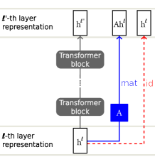
Figure 1: An illustration of our method $\texttt{mat}_{\ell\rightarrow\ell^{\prime}}{}$ (in blue) of short-cutting away transformer inference in-between certain layers by applying a matrix $A=A_{\ell^{\prime},\ell}$ learnt by fitting linear regression, versus the baseline method $\texttt{id}_{\ell\rightarrow\ell^{\prime}}{}$ (in red) of propagating the hidden representation as-is to the further layer.

Previous attempts to exploit hidden representations viewed the hidden representations of an input token as a sequence of approximations of its final representation Elhage et al. (2021); Geva et al. (2022b). This view is motivated by the additive updates induced via the residual connections He et al. (2016) around each layer in the network. Indeed, previous works Geva et al. (2021, 2022a); Ram et al. (2022); Alammar (2021) followed a simplifying assumption that representations at any layer can be transformed into a distribution over the output vocabulary by the output embeddings. While this approach has proven to be surprisingly effective for interpretability Geva et al. (2022a); Dar et al. (2022) and computation efficiency Schuster et al. (2022); Xin et al. (2020); Schwartz et al. (2020), it oversimplifies the model’s computation and assumes that all the hidden layers in the network operate in the same space.

A natural question that arises is whether there is a more accurate way to cast hidden representations into final representation substitutes than simply interpreting them as they are. In this work, we tackle this question by learning linear transformations across layers in the network (illustrated in Fig. 1). Concretely, for any two layers $\ell<\ell^{\prime}$, we fit linear regression to transform hidden representations from layer $\ell$ to layer $\ell^{\prime}$. We show that this method, called mat, produces substantially more accurate approximations than the above-discussed identity mapping, dubbed id, applied in previous works (§3). This suggests that there is more linearity to transformer inference than could be explained solely by the residual connection structure.

We further test our approach in the context of language modeling (§4), checking how often predictions from final representation substitutes produced by mat agree with those of actual final representations. Experiments across two data sources and different scales of GPT-2 Radford et al. (2019) and BERT Devlin et al. (2019) show large accuracy gains ($15\%$-$40\%$ at most layers) in prediction estimation by mat over naive projections (id). Moreover, we observe that our mappings often (in $>30\%$ of the cases) produce correct predictions when applied to the very early layers in the network.

We then leverage these findings for improving model efficiency and demonstrate our method’s utility in the setting of early exiting, a strategy according to which one dynamically decides at which layer to stop the inference pass and use that layer’s representation as a final layer representation substitute. While previous works have utilized these hidden representations intact (i.e. using id), we transform them using mat, showing that our method performs better than the baseline in this setting as well (§5), allowing for the saving of additional $7.9\%$ (resp. $5.4\%$) of the layers for GPT-2 (resp. BERT) when aiming at $95\%$ accuracy.

Last, we analyze how well different parts of the transformer computation can be estimated linearly (§6). To this end, we apply the same methodology to replace the sub-modules of attention, FFN, and layer normalization with linear mappings. Interestingly, we find that linearly approximating attention, the only sub-module in the network that has contextual processing, results in the least reduction of precision. This hints at an interesting possibility of compute time reduction, since non-contextual inference is parallelizable.

To conclude, we propose a method for casting hidden representations across transformer layers, that is light to train, cheap to infer, and provides more accurate representation approximations than the hitherto implicitly accepted baseline of identical propagation. The method is not only appealing for model analysis but also has concrete applications for efficiency.

2 Background and Notation

The input to a transformer-based LM Vaswani et al. (2017) is a sequence of tokens $t_{1},...,t_{n}$ from a vocabulary $\mathcal{V}$ of size $|\mathcal{V}|=d_{v}$. The tokens are first represented as vectors using an embedding matrix $E\in\mathbb{R}^{d_{h}\times d_{v}}$, where $d_{h}$ is the hidden dimension of the model, to create the initial hidden representations

$$H^{0}=(h_{1}^{0},\ldots,h_{n}^{0})\in\mathbb{R}^{d_{h}\times n}.$$

These representations are then repeatedly transformed through $L$ transformer blocks, where each block outputs hidden representations that are the inputs to the next block:

$$\forall\ell\in[1,L]:\;\;\texttt{b}^{\ell}(H^{\ell-1})=H^{\ell}$$

where

$$H^{\ell}=(h^{\ell}_{1},\ldots,h^{\ell}_{n})\in\mathbb{R}^{d_{h}\times n}.$$

The $\ell$-th transformer block is constructed as a composition of two layers:

$$\texttt{b}_{\ell}=\texttt{b}^{\texttt{ffn}}_{\ell}\circ\texttt{b}^{\texttt{attn}}_{\ell},$$

where $\texttt{b}^{\texttt{attn}}_{\ell}$ (resp. $\texttt{b}^{\texttt{ffn}}_{\ell}$) is a multi-head self-attention layer (resp. FFN layer) enclosed by a residual connection, and potentially interjected with layer normalization Ba et al. (2016).

The final representations, denoted as

$$H^{L}=(h_{1}^{L},\ldots,h_{n}^{L}),$$

are considered as the transformer stack’s output. These representations are used to form various predictions. In this work, we investigate whether and how hidden representations from earlier layers can be utilized for this purpose instead.

3 Linear Shortcut Across Blocks

To use a hidden representation from layer $\ell<L$ as a final representation, we propose to cast it using linear regression, while skipping the computation in-between these layers. More generally, this approach can be applied to cast any $\ell$-th hidden representation to any succeeding layer $\ell^{\prime}>\ell$.

3.1 Method

Given a source layer $\ell$ and a target layer $\ell^{\prime}$ such that $\ell<\ell^{\prime}\leq L$, our goal is to learn a mapping $A_{\ell^{\prime},\ell}\in\mathbb{R}^{d_{h}\times d_{h}}$ from hidden representations at layer $\ell$ to those at layer $\ell^{\prime}$. To this end, we first collect a set of corresponding hidden representation pairs $(h^{\ell},h^{\ell^{\prime}})$. Concretely, we run a set $\mathcal{T}$ of input sequences through the model, and for each such input $s$ we extract the hidden representations $h_{i_{s}}^{\ell},h_{i_{s}}^{\ell^{\prime}}$, where $i_{s}$ is a random position in $s$.

Next, we learn a matrix $A_{\ell^{\prime},\ell}\in\mathbb{R}^{d_{h}\times d_{h}}$ by fitting linear regression over $\mathcal{T}$, namely, $A_{\ell^{\prime},\ell}$ is a numerical minimizer for:

$$A\mapsto\sum_{s\in\mathcal{T}}||A\cdot h_{i_{s}}^{\ell}-h_{i_{s}}^{\ell^{\prime}}||^{2}.$$

We define the mapping of a representation $h$ from layer $\ell$ to layer $\ell^{\prime}$ as:

$$\texttt{mat}_{\ell\rightarrow\ell^{\prime}}{}(h)\coloneqq A_{\ell^{\prime},\ell}\cdot h$$ (1)

3.2 Baseline

We evaluate our method against the prevalent approach of “reading” hidden representations directly, without any transformation. Namely, the propagation of a hidden representation from layer $\ell$ to layer $\ell^{\prime}$ is given by the identity function, dubbed id:

$$\texttt{id}_{\ell\rightarrow\ell^{\prime}}{}(h)\coloneqq h.$$

Notably, this commonly-used baseline assumes that representations at different layers operate in the same linear space.

3.3 Quality of Fit

We first evaluate our method by measuring how well the learned linear mappings approximate the representations at the target layer. To this end, we calculate the (coordinate-averaged) $r^{2}$-score of our mapping’s outputs with respect to the “real” representations obtained from a full inference pass, and compare to the same for the id baseline.

Models.

We use GPT-2 Radford et al. (2019), a decoder-only auto-regressive LM, and BERT Devlin et al. (2019), an encoder-only model trained with masked language modeling. We conduct our evaluation over multiple scales of these models, with $12$, $24$, $36$, and $48$ layers for GPT-2, and $12$ and $24$ layers for BERT. The plots presented in this section are for $48$-layered GPT-2 and $24$-layered BERT; in §D we gather the plots for the rest of the models.

Data.

We use two data sources to evaluate our method – Wikipedia and news articles in English from the Leipzig Corpora Collection Goldhahn et al. (2012). From each source, we take 9,000 random sentences for training ($\mathcal{T}$). As a validation set, $\mathcal{V}$, we use additional 3,000 and 1,000 instances from Wikipedia and the Leipzig Corpora, respectively. For each example $s$, we select a random position $i_{s}$ and extract the hidden representations $h_{i_{s}}^{\ell}$ at that position from all the layers. For BERT, we convert the input token at position $i_{s}$ to a [MASK] token, as our main motivation is to interpret predictions, which are generated through masked tokens in BERT (see §4.2). Thus, the hidden representations we consider in the case of BERT are just of [MASK] tokens.

As we observed similar results for the two data sources across all our experiments, throughout the paper we will report results for Wikipedia and provide the results for the news articles in §B. Further details on the data and models are provided in §A.

Evaluation.

For every pair of layers $\ell,\ell^{\prime}$, such that $0\leq\ell<\ell^{\prime}\leq L$, we use the training set $\mathcal{T}$ to fit linear regression as described in §3.1, and obtain a mapping $\texttt{mat}_{\ell\rightarrow\ell^{\prime}}{}$. Next, we evaluate the quality of $\texttt{mat}_{\ell\rightarrow\ell^{\prime}}{}$ as well as of $\texttt{id}_{\ell\rightarrow\ell^{\prime}}{}$ using the $r^{2}$-coefficient, uniformly averaged over all coordinates. Concretely, we compute the $r^{2}$-coefficient of the true representations $h_{i_{s}}^{\ell^{\prime}}$ versus each of the predicted representations $\texttt{mat}_{\ell\rightarrow\ell^{\prime}}{}(h_{i_{s}}^{\ell})$ and $\texttt{id}_{\ell\rightarrow\ell^{\prime}}{}(h_{i_{s}}^{\ell})$ for every $s\in\mathcal{V}$.

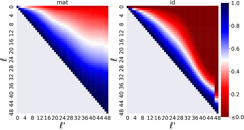
Figure 2: The coordinate-averaged $r^{2}$-score of $\texttt{mat}_{\ell\rightarrow\ell^{\prime}}{}$ (left) and $\texttt{id}_{\ell\rightarrow\ell^{\prime}}{}$ (right) ($48$-layered GPT-2).

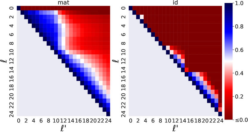
Figure 3: The coordinate-averaged $r^{2}$-score of $\texttt{mat}_{\ell\rightarrow\ell^{\prime}}{}$ (left) and $\texttt{id}_{\ell\rightarrow\ell^{\prime}}{}$ (right) ($24$-layered BERT masked inputs).

Results.

Results for $48$-layered GPT-2 and $24$-layered BERT are presented in Fig. 2 and 3, respectively. In both models, mat consistently yields better approximations than id, as it obtains higher $r^{2}$-scores (in blue) across the network.

This gap between mat and id is especially evident in BERT, where id completely fails to map the representations between most layers, suggesting that hidden representations are modified substantially by every transformer block. Overall, this highlights the shortcoming of existing practices to inspect representations in the same linear space, and the gains from using our method to approximate future layers in the network.

4 Linear Shortcut for Language Modeling

We saw that our method approximates future hidden representations substantially better than a naive propagation. In this section, we will show that this improvement also translates to better predictive abilities from earlier layers. Specifically, we will use our method to estimate how often intermediate representations encode the final prediction, in the context of two fundamental LM tasks; next token prediction and masked token prediction.

Evaluation Metrics.

Let $h,h^{\prime}\in\mathbb{R}^{d_{h}}$ be a final representation and a substitute final representation obtained by some mapping, and denote by $\delta(h),\delta(h^{\prime})\in\mathbb{R}^{d_{v}}$ their corresponding output probability distributions (obtained through projection to the output vocabulary – see details below). We measure the prediction quality of $h^{\prime}$ with respect to $h$ using two metrics:

• Precision@$k$ ($\uparrow$ is better): This checks whether the token with the highest probability according to $\delta(h^{\prime})$ appears in the top-$k$ tokens according to $\delta(h)$. Namely, we sort $\delta(h)$ and assign a score of $1$ if $\arg\max(\delta(h^{\prime}))$ appears in the top-$k$ tokens by $\delta(h)$, and $0$ otherwise.

• Surprisal ($\downarrow$ is better): We measure the minus log-probability according to $\delta(h)$, of the highest-probability token according to $\delta(h^{\prime})$. Intuitively, low values mean that the model sees the substitute result as probable and hence not surprising.

We report the average Precision@$k$ and Surprisal over the validation set $\mathcal{V}$.

4.1 Next Token Prediction

Auto-regressive LMs output for every position a probability distribution over the vocabulary for the next token. Specifically, the output distribution for every position $i$ is given by $\delta(h_{i}^{L})$, where:

$$\delta(h)=\texttt{softmax}(E^{\top}\cdot h)\in\mathbb{R}^{d_{v}}$$ (2)

For some LMs, including GPT-2, a layer normalization ln_f is applied to the final layer representation before this conversion (i.e., computing $\delta(\texttt{ln\_f}(h))$ rather than $\delta(h)$).

Recall that our goal is to measure how well this distribution can be estimated from intermediate representations, i.e. estimating $\delta(h_{i}^{L})$ from $\delta(h_{i}^{\ell})$ where $\ell<L$. To this end, we first run examples from the validation set through the model, while extracting for each example $s$ the hidden representation of a random position $i_{s}$ at every layer. Next, we apply our mappings $\texttt{mat}_{\ell\rightarrow L}{}$ and the $\texttt{id}_{\ell\rightarrow L}{}$ baseline to cast the hidden representations of every layer $\ell$ to final layer substitutes (see §3). Last, for each layer, we convert its corresponding final-layer substitute to an output distribution (Eq. 2) and compute the average Precision@$k$ (for $k=1,5,10$) and Surprisal scores with respect to the final output distribution, over the validation set.

Results.

Figs. 4 and 5 show the average Precision@$k$ and Surprisal scores per layer in $48$-layered GPT-2, respectively (the plots for the other GPT-2 models are presented in §D). Across all layers, mat outperforms id in terms of both scores, often by a large margin (e.g. till layer $44$ the Precision@$1$ achieved by mat is bigger than that of id by more than $0.2$). This shows that linear mappings enable not just better estimation of final layer representations, but also of the predictions they induce. Moreover, the relatively high Precision@$k$ scores of mat in early layers ($0.62$-$0.82$ for $k=10$, $0.52$-$0.74$ for $k=5$, and $0.28$-$0.45$ for $k=1$) suggest that early representations already encode a good estimation of the final prediction. Also, the substantially lower Surprisal scores of mat compared to id imply that our method allows for a more representative reading into the layer-wise prediction-formation of the model than allowed through direct projection to the vocabulary.

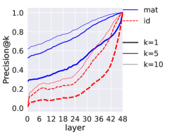
Figure 4: Precision@$k$ ($k=1,5,10$) of $\texttt{mat}_{\ell\rightarrow L}{}$ and $\texttt{id}_{\ell\rightarrow L}{}$ for next token prediction in $48$-layered GPT-2.

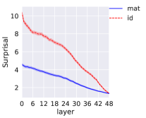
Figure 5: Surprisal for $\texttt{mat}_{\ell\rightarrow L}$ and the baseline $\texttt{id}_{\ell\rightarrow L}{}$ ($48$-layered GPT-2 next token prediction task). A 95% confidence interval surrounds the lines.

4.2 Masked Token Prediction

We now conduct the same experiment for the task of masked language modeling, where the model predicts a probability distribution of a masked token in the input rather than the token that follows the input. Unlike next token prediction, where the output distribution is computed from representations of varying input tokens, in masked token prediction the output is always obtained from representations of the same input token (i.e. [MASK]).

For this experiment, we use BERT, on top of which we use a pretrained masked language model head $\delta$; given a token sequence $s$, a [MASK] token inside it and its final representation $h$, $\delta(h)\in\mathbb{R}^{d_{v}}$ is a probability distribution over tokens giving the model’s assessment of the likelihood of tokens to be fitting in place of the [MASK] token in $s$.

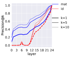
Figure 6: Precision@$k$ ($k=1,5,10$) for $\texttt{mat}_{\ell\rightarrow L}{}$ and the baseline $\texttt{id}_{\ell\rightarrow L}{}$ ($24$-layered BERT masked token prediction task).

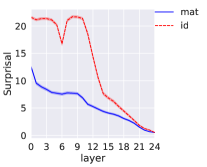
Figure 7: Surprisal for $\texttt{mat}_{\ell\rightarrow L}{}$ and the baseline $\texttt{id}_{\ell\rightarrow L}{}$ ($24$-layered BERT masked token prediction task). A 95% confidence interval surrounds the lines.

Results.

Figs. 6 and 7 present the average Precision@$k$ and Surprisal scores per layer in $24$-layered BERT (the plots for the $12$-layered BERT model are presented in §D), overall showing trends similar to those observed for next token prediction in GPT-2 (§4.1). This is despite the differences between the two tasks and the considerable architectural differences between BERT and GPT-2. Notably, the superiority of mat over id in this setting is even more prominent; while mat’s precision is between $0.2-0.6$ in the first ten layers (Fig. 6), id’s precision for all values of $k$ is close to zero, again strongly indicating that our method allows for better reading into early layer hidden representations. More generally, mat improves the Precision@$1$ of id by more than $17\%$ at most layers, and unveils that a substantial amount of predictions ($>25\%$ starting from layer $3$) appear already in the very first layers. Interestingly, the (rough) divide between the first half of layers and last half of layers for id in Figs. 6, 7 seems to align with the two-hump shape of the blue region for mat in Fig. 3.

Analysis.

We manually compare the predictions of our mapping $\texttt{mat}_{\ell\rightarrow L}{}$ with $\texttt{id}_{\ell\rightarrow L}{}$, for a $24$-layered BERT model. Concretely, we select 50 random sentences from the Leipzig dataset. Next, for each layer $\ell$, we manually analyze how many of the top-$5$ tokens according to $\texttt{mat}_{\ell\rightarrow L}{}$ and $\texttt{id}_{\ell\rightarrow L}{}$ fit into context. We consider a token to fit into context if it is grammatically plausible within the sentence (see Tab. 1 for concrete examples). In the resulting $1250$ instances (i.e. $50$ sentences $\times$ $25$ representations), we observe a substantially higher plausibility rate of $85.36\%$ for mat compared to $52.8\%$ for id. In fact, only in less than $4.3\%$ of the instances there are more plausible tokens among the top-$5$ tokens according to id than among the top-$5$ tokens according to mat, further supporting the Surprisal results above.

	$\texttt{id}_{4\rightarrow 24}$	$\texttt{mat}_{4\rightarrow 24}$	$\texttt{id}_{12\rightarrow 24}$	$\texttt{mat}_{12\rightarrow 24}$	$\texttt{id}_{24\rightarrow 24}$
aldridge had shoulder surgery in [MASK].	fellowship		cyclist
	employment		emergencies
	agreement	her	seniors
	##ostal	them	cycling
	##com	work
on your next view you will be asked to [MASK] continue reading.	##com	be	be	be
	accreditation	get	undergo
	$\copyright$	go	spartans	help
	fellowship		seniors
	summer	have	*	say

Table 1: Examples of top-$5$ predictions at layers $4$, $12$ and $24$, under the mappings $\texttt{mat}_{\ell\rightarrow L}{}$ and $\texttt{id}_{\ell\rightarrow L}{}$, for a $24$-layered BERT model. Grammatically plausible predictions (according to a human annotator) are marked in . Note that at layer $24$ the predictions of $\texttt{mat}_{\ell\rightarrow L}{}$ and $\texttt{id}_{\ell\rightarrow L}{}$ are the same (by definition).

5 Implication to Early Exiting

The fact that it is often possible to approximate the final prediction already from early layers in the network has important implications to efficiency. Concretely, applying our linear mapping instead of executing transformer blocks of quadratic time complexity, could potentially save a substantial portion of the computation. In this section, we demonstrate this in the context of early exiting.

When performing transformer model inference under an early exit strategy Schwartz et al. (2020); Xin et al. (2020); Schuster et al. (2022), one aims at deciding dynamically at which layer, during inference, to stop the computation and “read” the prediction from the hidden representation of that layer. More precisely, under the confidence measure paradigm, one decides to stop the computation for a position $i$ at layer $\ell$ based on a confidence criterion, that is derived from casting the hidden representation $h_{i}^{\ell}$ as a final-layer representation and converting it to an output probability distribution. Specifically, following Schuster et al. (2022), a decision to stop the computation is made if the difference between the highest and the second highest probabilities is bigger than

$$0.9\cdot\lambda+0.1\cdot{\rm exp}(-4i/N),$$

where $N$ is the average length of the input until position $i_{s}$ for $s\in\mathcal{V}$, and $\lambda$ is a confidence hyper-parameter.

Experiment.

We assess the utility of our mapping $\texttt{mat}_{\ell\rightarrow L}{}$ for early exit as a plug-and-play replacement for the $\texttt{id}_{\ell\rightarrow L}{}$ mapping, through which intermediate representations are cast into final-layer representations. In our experiments, we use both ($24$-layered) GPT-2 for the next token prediction and ($24$-layered) BERT for masked token prediction. We run each of the models over the validation set examples, while varying the confidence parameter $\lambda$ (see the exact values in §A.3) and using either $\texttt{id}_{\ell\rightarrow L}{}$ or $\texttt{mat}_{\ell\rightarrow L}{}$ for casting intermediate representations. Furthermore, we compare these early exit variants to the “fixed exit” strategy from §4, where the computation is stopped after a pre-defined number of layers rather than relying on a dynamic decision.

We evaluate each variant in terms of both prediction’s accuracy, using the Precision@$1$ metric (see §4), and efficiency, measured as the average number of layers processed during inference.

Results.

Figs. 8 and 9 plot the average Precision@$1$ score against the average number of layers processed, for $24$-layered GPT-2 and $24$-layered BERT, respectively. For both models, under an early exit strategy our mapping mat again provides a substantial improvement over the baseline id. For example, aiming at $95\%$ average precision, mat saves $\sim 3.3$ ($13.8$%) layers in GPT-2 compared to only $\sim 1.4$ ($5.9$%) layers by id, and $\sim 4.8$ ($20$%) layers in BERT versus $\sim 3.5$ ($14.6$%) layers by id. These results highlight to potential gains prominent early exit methods can obtain by using our method. Notably, in both models and using each of the two mapping methods, early exit obtains better results than fixed layer exit, as expected.

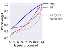
Figure 8: Precision@$1$ for the various early exit methods, and previous “fixed exit” methods for comparison ($24$-layered GPT-2 next token prediction task). Varying the confidence parameter $\lambda$, the $x$-coordinate is the average number of layers processed before an early exit decision is reached.

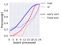
Figure 9: Precision@$1$ for the various early exit methods, and previous fixed exit methods for comparison ($24$-layered BERT masked token prediction task). Varying the confidence parameter $\lambda$, the $x$-coordinate is the average number of layers processed before an early exit decision is reached.

6 Linear Shortcut Across Sub-modules

Our experiments show that, despite the commonly-applied simplification by interpretability works, transformer layers do not operate in the same linear space and there is a major gap in approximating future representations using an identity mapping (§3, §4). In this section, we investigate whether discrepancies across layers result from specific sub-modules or are a general behaviour of all sub-modules in the network.

This is done by extending our approach to test how well particular components in transformer blocks can be linearly approximated.

Method.

Discussing GPT-2 for definiteness, we have

$$\texttt{b}_{\ell}=\texttt{b}_{\ell}^{\texttt{ffn}}\circ\texttt{b}_{\ell}^{\texttt{attn}}$$

with

$$\texttt{b}^{\texttt{attn}}_{\ell}(H)=\texttt{attn}_{\ell}(\texttt{ln1}_{\ell}(H))+H,$$ (3)

where $\texttt{attn}_{\ell}$ is a multi-head self-attention layer and ln1 is a layer normalization, and

$$\texttt{b}^{\texttt{ffn}}_{\ell}(H)=\texttt{ffn}_{\ell}(\texttt{ln2}_{\ell}(H))+H,$$

where $\texttt{ffn}_{\ell}$ is a feed-forward network layer and ln2 is a layer normalization.

Given a block $\texttt{b}_{\ell}$ and one of its sub-modules $\texttt{ln1}_{\ell},\ \texttt{attn}_{\ell},\ \texttt{ln2}_{\ell}$, or $\texttt{ffn}_{\ell}$, we fit a linear regression approximating the output of the sub-module given its input. Illustrating this on $\texttt{attn}_{\ell}$ for definiteness, let $v^{\ell}_{i_{s}}$ be the vector at position $i_{s}$ in the output of $\texttt{attn}_{\ell}(\texttt{ln1}_{\ell}(H^{\ell-1}))$, for a given input $s$. We denote by $A_{\ell}^{\texttt{attn}}\in\mathbb{R}^{d_{h}\times d_{h}}$ the matrix numerically minimizing

$$A\mapsto\sum_{s\in\mathcal{T}}||A\cdot\texttt{ln1}_{\ell}(h^{\ell-1}_{i_{s}})-v^{\ell}_{i_{s}}||^{2},$$

and define a replacement of the attention sub-module (Eq. 3) by

$$\texttt{b}^{\overline{\texttt{attn}}}_{\ell}(h)\coloneqq A_{\ell}^{\texttt{attn}}\cdot\texttt{ln1}_{\ell}(h)+h.$$ (4)

We then define a mapping between two layers ${\ell\rightarrow\ell^{\prime}}$ by:

$$\texttt{mat\_attn}_{\ell\rightarrow\ell^{\prime}}{}(h)\coloneqq$$

$$\texttt{b}^{\texttt{ffn}}_{\ell^{\prime}}(\texttt{b}^{\overline{\texttt{attn}}}_{\ell^{\prime}}(\ldots(\texttt{b}^{\texttt{ffn}}_{\ell+1}(\texttt{b}^{\overline{\texttt{attn}}}_{\ell+1}(h))\ldots)).$$

In other words, when applying each $\ell^{\prime\prime}$-th block, $\ell<\ell^{\prime\prime}\leq\ell^{\prime}$, we replace its attention sub-module $\texttt{attn}_{\ell^{\prime\prime}}$ by its linear approximation.

In an analogous way, we consider the mappings $\texttt{mat\_ffn}_{\ell\rightarrow\ell^{\prime}}{}$ and $\texttt{mat\_ln1\_ln2}_{\ell\rightarrow\ell^{\prime}}{}$, where in the latter we perform the linear shortcut both for ln1 and for ln2 (see §C for precise descriptions). Importantly, unlike the original attention module, the approximation $\texttt{b}^{\overline{\texttt{attn}}}_{\ell}$ operates on each position independently, and therefore, applying the mapping $\texttt{mat\_attn}_{\ell\rightarrow\ell^{\prime}}{}$ disables any contextualization between the layers $\ell$ and $\ell^{\prime}$. Note that this is not the case for $\texttt{mat\_ffn}_{\ell\rightarrow\ell^{\prime}}{}$ and $\texttt{mat\_ln1\_ln2}_{\ell\rightarrow\ell^{\prime}}{}$, which retain the self-attention sub-modules and therefore operate contextually.

Evaluation.

We analyze the $24$-layered GPT-2, and proceed completely analogously to §4.1, evaluating the Precision@$k$ and Surprisal metrics for the additional mappings $\texttt{mat\_attn}_{\ell\rightarrow L}{}$, $\texttt{mat\_ffn}_{\ell\rightarrow L}{}$ and $\texttt{mat\_ln1\_ln2}_{\ell\rightarrow L}{}$.

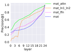
Figure 10: Precision@$1$ for the various sub-module linear shortcut mappings, and the mapping $\texttt{mat}_{\ell\rightarrow L}{}$ for comparison (GPT-2 next token prediction task).

Figure 11: Surprisal for the various sub-module linear shortcut mappings, and the mapping $\texttt{mat}_{\ell\rightarrow L}{}$ for comparison (GPT-2 next token prediction task). A 95% confidence interval surrounds the lines.

Results.

Figs. 10 and 11 show the average Precision@$1$ and Surprisal scores per layer in the $24$-layered GPT-2, respectively. However, from a certain layer (~$7$), all sub-module mappings achieve better results than the full-block mapping $\texttt{mat}_{\ell\rightarrow L}{}$. Thus, it is not just the cumulative effect of all the sub-modules in the transformer block that is amenable to linear approximation, but also individual sub-modules can be linearly approximated. Our experiments expose further that the linear approximation of attention sub-modules is much less harmful than that of the FFN or layer normalization sub-modules. Hypothetically, a possible reason is that the linear replacement of FFN or layer normalization “erodes” the self-attention computation after a few layers. Moreover, the good performance of $\texttt{mat\_attn}_{\ell\rightarrow L}{}$ suggests that in many cases the consideration of context exhausts itself early in the procession of layers; speculatively, it is only in more delicate cases that the self-attention of late layers adds important information. Last, remark the sharp ascent of the results of the layer normalization mapping between layers $5$-$8$, for which we do not currently see a particular reason. To conclude, we learn that the possibility of linear approximation permeates the various transformer components.

7 Related Work

Recently, there was a lot of interest in utilizing intermediate representations in transformer-based LMs, both for interpretability and for efficiency.

In the direction of interpretability, one seeks to understand the prediction construction process of the model Tenney et al. (2019); Voita et al. (2019).

More recent works use mechanistic interpretability and view the inference pass as a residual stream of information Dar et al. (2022); Geva et al. (2022b). Additionally, there are works on probing, attempting to understand what features are stored in the hidden representations Adi et al. (2017); Conneau et al. (2018); Liu et al. (2019). Our work is different in that it attempts to convert intermediate representations into a final-layer form, which is interpretable by design.

In the direction of efficiency, there is the thread of work on early exit, where computation is cut at a dynamically-decided earlier stage Schwartz et al. (2020); Xin et al. (2020); Schuster et al. (2022). Other works utilize a fixed early stage network to parallelize inference (Leviathan et al., 2022; Chen et al., 2023). However, intermediate representations are directly propagated in these works, which we show is substantially worse than our approach. Moreover, our method requires training considerably less parameters than methods such as Schuster et al. (2021), that learn a different output softmax for each intermediate layer.

More broadly, skipping transformer layers and analyzing the linearity properties of transformer components have been discussed in prior works Zhao et al. (2021); Mickus et al. (2022); Wang et al. (2022); Lamparth and Reuel (2023).

8 Conclusion and Future Work

We present a simple method for inspection of hidden representations in transformer models, by using pre-fitted context-free and token-uniform linear mappings. Through a series of experiments on different data sources, model architectures and scales, we show that our method consistently outperforms the prevalent practice of interpreting representations in the final-layer space of the model, yielding better approximations of succeeding representations and the predictions they induce.

We also demonstrate the practicality of our method for improving computation efficiency, saving a substantial amount of compute on top of prominent early exiting approaches.

Last, by extending our method to sub-modules, more specifically the attention sub-modules, we observe that in some cases replacing a part of transformer inference by a non-contextual linear computation only results in a small deterioration of the prediction. This opens new research directions for improving model efficiency, including breaking the computation into several parallelizable tasks.

Limitations

Although we see in this work that there is more linear structure to transformer inference than could be explained solely by the residual connection, we do not elucidate a reason for that. We also do not try to formulate formal criteria according to which to judge, in principle, the quality of ways of short-cutting transformer inference in-between layers. In addition, our experiments cover only English data.

Appendix A Experimental Setup Details

Here we specify the experimental setup details.

A.1 Models

GPT-2.

We use the four versions of the GPT-2 model from Huggingface Wolf et al. (2020), having $L=12,24,36,48$ hidden layers and hidden dimensions $d_{h}=768,1024,1280,1600$ respectively.

BERT.

We use the bert-large-uncased model from Huggingface, having $L=24$ hidden layers and hidden dimension $d_{h}=1024$, and the bert-base-uncased model from Huggingface, having $L=12$ hidden layers and hidden dimension $d_{h}=768$. We use the BertForMaskedLM heads from Huggingface, pretrained for these models.

A.2 Data

When experimenting on the Wikipedia dataset, to generate an input sequence for our training and validation sets, we pick a random document from the Wikipedia dataset from Huggingface, use spaCy to break the document into sentences and pick a random sentence ending with a newline character among those.

When experimneting on the news article sentences dataset, we use the 10K English 2020 news sentences corpus from the Leipzig Corpora Collection, which we randomly divide into a training set $\mathcal{T}$ consisting of 9,000 examples and a validation set $\mathcal{V}$ consisting of 1,000 examples.

In the GPT-2 (resp. BERT) experiment, a tokenized sentence with more than 1024 (resp. 512) tokens was truncated to have 1024 (resp. 512) tokens.

A.3 Values of $\lambda$ Used in §5

In §5, to have a plot which is gradual enough, we use the following values of $\lambda$:

• $\{-1.112\}\cup\{0.1\cdot i\ :0\leq i\leq 10\}\cup\{1.112\}$.

• For the baseline method id, to the values above we also add

  $$\{1+0.0112\cdot i\ :\ 0<i<10\}.$$

Appendix B Results on News Articles Data

Here we record the results of the main experiments when evaluated on the Leipzig Corpora news article sentences dataset, in Figs. 12, 13 (quality of fit), Figs. 14, 15, 16, 17 (linear shortcut for language modeling), Figs. 18, 19 (linear shortcut across sub-modules in blocks) and Figs. 20, 21 (early exit).

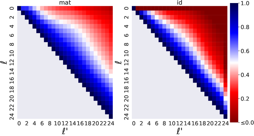
Figure 12: The coordinate-averaged $r^{2}$-score of $\texttt{mat}_{\ell\rightarrow\ell^{\prime}}{}$ (left) and $\texttt{id}_{\ell\rightarrow\ell^{\prime}}{}$ (right) ($24$-layered GPT-2) - Leipzig dataset.

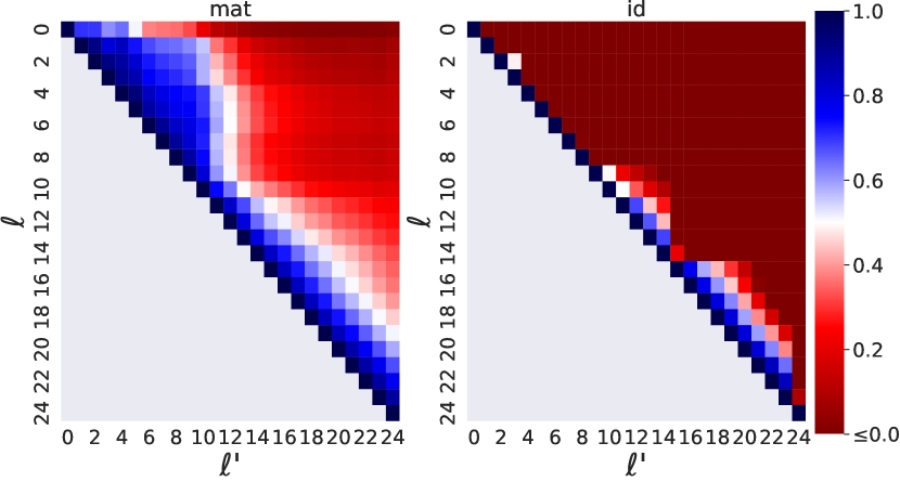
Figure 13: The coordinate-averaged $r^{2}$-score of $\texttt{mat}{}_{\ell^{\prime},\ell}$ (left) and $\texttt{id}_{\ell\rightarrow\ell^{\prime}}{}$ (right) ($24$-layered BERT masked inputs) - Leipzig dataset.

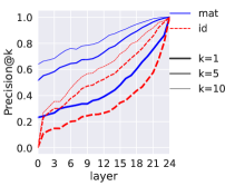
Figure 14: Precision@$k$ ($k=1,5,10$) for $\texttt{mat}_{\ell\rightarrow L}{}$ and the baseline $\texttt{id}_{\ell\rightarrow L}{}$ ($24$-layered GPT-2 next token prediction task) - Leipzig dataset.

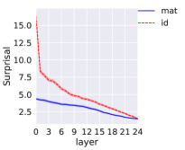
Figure 15: Surprisal for $\texttt{mat}_{\ell\rightarrow L}{}$ and the baseline $\texttt{id}_{\ell\rightarrow L}{}$ ($24$-layered GPT-2 next token prediction task) - Leipzig dataset.

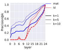
Figure 16: Precision@$k$ for $\texttt{mat}_{\ell\rightarrow L}{}$ and the baseline $\texttt{id}_{\ell\rightarrow L}{}$ ($24$-layered BERT masked token prediction task) - Leipzig dataset.

Figure 17: Surprisal for $\texttt{mat}_{\ell\rightarrow L}{}$ and the baseline $\texttt{id}_{\ell\rightarrow L}{}$ ($24$-layered BERT masked token prediction task) - Leipzig dataset.

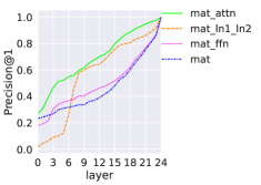
Figure 18: Precision@$1$ for the various sub-module linear shortcut mappings, and the mapping $\texttt{mat}_{\ell\rightarrow L}{}$ for comparison ($24$-layered GPT-2 next token prediction task) - Leipzig dataset.

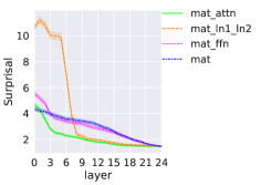
Figure 19: Surprisal for the various sub-module linear shortcut mappings, and the mapping $\texttt{mat}_{\ell\rightarrow L}{}$ for comparison ($24$-layered GPT-2 next token prediction task) - Leipzig dataset.

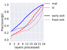
Figure 20: Precision@$1$ for the various early exit methods, and previous fixed exit methods for comparison ($24$-layered GPT-2 next token prediction task) - Leipzig dataset. Varying the confidence parameter $\lambda$, the $x$-coordinate is the average number of layers processed before an early exit decision is reached.

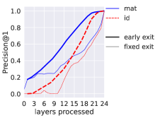
Figure 21: Precision@$1$ for the various early exit methods, and previous fixed exit methods for comparison ($24$-layered BERT masked token prediction task) - Leipzig dataset. Varying the confidence parameter $\lambda$, the $x$-coordinate is the average number of layers processed before an early exit decision is reached.

Appendix C Descriptions of $\texttt{mat\_ffn}_{\ell\rightarrow\ell^{\prime}}{}$ and $\texttt{mat\_ln1\_ln2}_{\ell\rightarrow\ell^{\prime}}{}$

Here we detail the definitions of the mappings $\texttt{mat\_ffn}_{\ell\rightarrow\ell^{\prime}}{}$ and $\texttt{mat\_ln1\_ln2}_{\ell\rightarrow\ell^{\prime}}{}$ utilized in §6.

Description of $\texttt{mat\_ffn}_{\ell\rightarrow\ell^{\prime}}{}$.

Let $v^{\ell}_{i_{s}}$ be the vector at position $i_{s}$ in the output of $\texttt{ln2}_{\ell}(\texttt{b}_{\ell}^{\texttt{attn}}(H^{\ell-1}))$, for a given input $s$. We denote by $A_{\ell}^{\texttt{ffn}}\in\mathbb{R}^{d_{h}\times d_{h}}$ the matrix numerically minimizing

$$A\mapsto\sum_{s\in\mathcal{T}}||A\cdot v^{\ell}_{i_{s}}-\texttt{ffn}_{\ell}(v^{\ell}_{i_{s}})||^{2},$$

and define a replacement of the feed-forward sub-module $\texttt{b}_{\ell}^{\texttt{ffn}}$ by

$$\texttt{b}^{\overline{\texttt{ffn}}}_{\ell}(H)\coloneqq A_{\ell}^{\texttt{ffn}}\cdot\texttt{ln2}_{\ell}(H)+H.$$

We then define a mapping between two layers ${\ell\rightarrow\ell^{\prime}}$ by:

$$\texttt{mat\_ffn}_{\ell\rightarrow\ell^{\prime}}{}(H)\coloneqq$$

$$\texttt{b}^{\overline{\texttt{ffn}}}_{\ell^{\prime}}(\texttt{b}^{\texttt{attn}}_{\ell^{\prime}}(\ldots(\texttt{b}^{\overline{\texttt{ffn}}}_{\ell+1}(\texttt{b}^{\texttt{attn}}_{\ell+1}(H))\ldots)).$$

Description of $\texttt{mat\_ln1\_ln2}_{\ell\rightarrow\ell^{\prime}}{}$.

Let $v^{\ell}_{i_{s}}$ be the vector at position $i_{s}$ in the output of $\texttt{b}^{\texttt{attn}}_{\ell}(H^{\ell-1})$, for a given input $s$. We denote by $A_{\ell}^{\texttt{ln1}}\in\mathbb{R}^{d_{h}\times d_{h}}$ the matrix numerically minimizing

$$A\mapsto\sum_{s\in\mathcal{T}}||A\cdot h^{\ell}_{i_{s}}-\texttt{ln1}_{\ell}(h^{\ell}_{i_{s}})||^{2}$$

and we denote by $A_{\ell}^{\texttt{ln2}}\in\mathbb{R}^{d_{h}\times d_{h}}$ the matrix numerically minimizing

$$A\mapsto\sum_{s\in\mathcal{T}}||A\cdot v^{\ell}_{i_{s}}-\texttt{ln2}_{\ell}(v^{\ell}_{i_{s}})||^{2}.$$

We define a replacement of the block $\texttt{b}^{\texttt{attn}}_{\ell}$ by

$$\texttt{b}^{\overline{\texttt{ln1}}}_{\ell}(H)\coloneqq\texttt{attn}_{\ell}(A_{\ell}^{\texttt{ln1}}\cdot H)+H$$ (5)

and we define a replacement of the block $\texttt{b}^{\texttt{ffn}}_{\ell}$ by

$$\texttt{b}^{\overline{\texttt{ln2}}}_{\ell}(H)\coloneqq\texttt{ffn}_{\ell}(A_{\ell}^{\texttt{ln2}}\cdot H)+H.$$ (6)

We then define a mapping between two layers ${\ell\rightarrow\ell^{\prime}}$ by:

$$\texttt{mat\_ln1\_ln2}_{\ell\rightarrow\ell^{\prime}}{}(H)\coloneqq$$

$$\texttt{b}^{\overline{\texttt{ln2}}}_{\ell^{\prime}}(\texttt{b}^{\overline{\texttt{ln1}}}_{\ell^{\prime}}(\ldots(\texttt{b}^{\overline{\texttt{ln2}}}_{\ell+1}(\texttt{b}^{\overline{\texttt{ln1}}}_{\ell+1}(H))\ldots)).$$

Appendix D Results for Models of Various Sizes

Here we record results of some of the experiments when performed with $12$, $24$ and $36$-layered versions of GPT-2 and $12$-layered version of BERT, on the Wikipedia dataset; Figs. 22, 23, 24, 25 (quality of fit), Figs. 26, 27, 28, 29 (layer linear shortcut, Precision@$k$), Figs. 30, 31, 32, 33 (layer linear shortcut, Surprisal),

Figure 22: The coordinate-averaged $r^{2}$-score of $\texttt{mat}_{\ell\rightarrow\ell^{\prime}}{}$ (left) and $\texttt{id}_{\ell\rightarrow\ell^{\prime}}{}$ (right) ($12$-layered GPT-2).

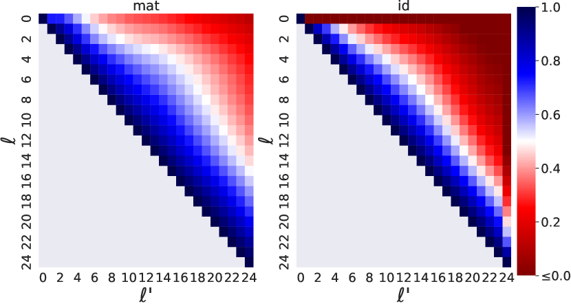
Figure 23: The coordinate-averaged $r^{2}$-score of $\texttt{mat}_{\ell\rightarrow\ell^{\prime}}{}$ (left) and $\texttt{id}_{\ell\rightarrow\ell^{\prime}}{}$ (right) ($24$-layered GPT-2).

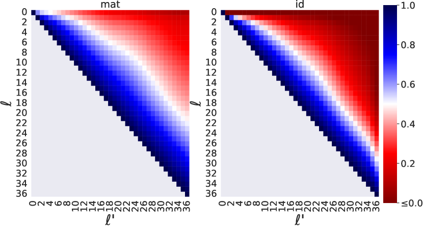
Figure 24: The coordinate-averaged $r^{2}$-score of $\texttt{mat}_{\ell\rightarrow\ell^{\prime}}{}$ (left) and $\texttt{id}_{\ell\rightarrow\ell^{\prime}}{}$ (right) ($36$-layered GPT-2).

Figure 25: The coordinate-averaged $r^{2}$-score of $\texttt{mat}_{\ell\rightarrow\ell^{\prime}}{}$ (left) and $\texttt{id}_{\ell\rightarrow\ell^{\prime}}{}$ (right) ($12$-layered BERT masked inputs).

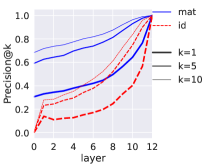
Figure 26: Precision@$k$ ($k=1,5,10$) for $\texttt{mat}_{\ell\rightarrow L}{}$ and the baseline $\texttt{id}_{\ell\rightarrow L}{}$ ($12$-layered GPT-2 next token prediction task).

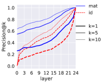
Figure 27: Precision@$k$ ($k=1,5,10$) for $\texttt{mat}_{\ell\rightarrow L}{}$ and the baseline $\texttt{id}_{\ell\rightarrow L}{}$ ($24$-layered GPT-2 next token prediction task).

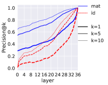
Figure 28: Precision@$k$ ($k=1,5,10$) for $\texttt{mat}_{\ell\rightarrow L}{}$ and the baseline $\texttt{id}_{\ell\rightarrow L}{}$ ($36$-layered GPT-2 next token prediction task).

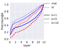
Figure 29: Precision@$k$ ($k=1,5,10$) for $\texttt{mat}_{\ell\rightarrow L}{}$ and the baseline $\texttt{id}_{\ell\rightarrow L}{}$ ($12$-layered BERT masked token prediction task).

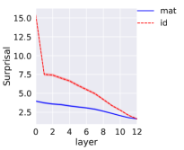
Figure 30: Surprisal for $\texttt{mat}_{\ell\rightarrow L}{}$ and the baseline $\texttt{id}_{\ell\rightarrow L}{}$ ($12$-layered GPT-2 next token prediction task).

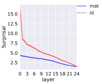
Figure 31: Surprisal for $\texttt{mat}_{\ell\rightarrow L}{}$ and the baseline $\texttt{id}_{\ell\rightarrow L}{}$ ($24$-layered GPT-2 next token prediction task).

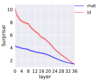
Figure 32: Surprisal for $\texttt{mat}_{\ell\rightarrow L}{}$ and the baseline $\texttt{id}_{\ell\rightarrow L}{}$ ($36$-layered GPT-2 next token prediction task).

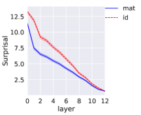
Figure 33: Surprisal for $\texttt{mat}_{\ell\rightarrow L}{}$ and the baseline $\texttt{id}_{\ell\rightarrow L}{}$ ($12$-layered BERT masked token prediction task).

Appendix E More Figures

Here we record Figs. 34, 35 mentioned in §6.

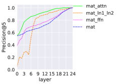
Figure 34: Precision@$5$ for the various sub-module linear shortcut methods, and the previous method mat for comparison ($24$-layered GPT-2 next token prediction task) - Wikipedia dataset. For a layer $\ell$, which serves as the $x$-coordinate, the $y$-coordinate is the rate at which the top $1$ token according to a method lies in the top $5$ tokens according to the model.

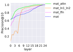
Figure 35: Precision@$10$ for the various sub-module linear shortcut methods, and the previous method mat for comparison ($24$-layered GPT-2 next token prediction task) - Wikipedia dataset. For a layer $\ell$, which serves as the $x$-coordinate, the $y$-coordinate is the rate at which the top $1$ token according to a method lies in the top $10$ tokens according to the model.

References

- Adi et al. (2017) Yossi Adi, Einat Kermany, Yonatan Belinkov, Ofer Lavi, and Yoav Goldberg. 2017. Fine-grained analysis of sentence embeddings using auxiliary prediction tasks. In International Conference on Learning Representations.
- Alammar (2021) J Alammar. 2021. Ecco: An open source library for the explainability of transformer language models. In Proceedings of the 59th Annual Meeting of the Association for Computational Linguistics and the 11th International Joint Conference on Natural Language Processing: System Demonstrations, pages 249–257, Online. Association for Computational Linguistics.
- Ba et al. (2016) Lei Jimmy Ba, Jamie Ryan Kiros, and Geoffrey E. Hinton. 2016. Layer normalization. CoRR, abs/1607.06450.
- Chen et al. (2023) Charlie Chen, Sebastian Borgeaud, Geoffrey Irving, Jean-Baptiste Lespiau, Laurent Sifre, and John Jumper. 2023. Accelerating large language model decoding with speculative sampling. arXiv preprint arXiv:2302.01318.
- Conneau et al. (2018) Alexis Conneau, German Kruszewski, Guillaume Lample, Loïc Barrault, and Marco Baroni. 2018. What you can cram into a single $&!#* vector: Probing sentence embeddings for linguistic properties. In Proceedings of the 56th Annual Meeting of the Association for Computational Linguistics (Volume 1: Long Papers), pages 2126–2136, Melbourne, Australia. Association for Computational Linguistics.
- Dar et al. (2022) Guy Dar, Mor Geva, Ankit Gupta, and Jonathan Berant. 2022. Analyzing transformers in embedding space. arXiv preprint arXiv:2209.02535.
- Devlin et al. (2019) Jacob Devlin, Ming-Wei Chang, Kenton Lee, and Kristina Toutanova. 2019. BERT: Pre-training of deep bidirectional transformers for language understanding. In Proceedings of the 2019 Conference of the North American Chapter of the Association for Computational Linguistics: Human Language Technologies, Volume 1 (Long and Short Papers), pages 4171–4186, Minneapolis, Minnesota. Association for Computational Linguistics.
- Elhage et al. (2021) Nelson Elhage, Neel Nanda, Catherine Olsson, Tom Henighan, Nicholas Joseph, Ben Mann, Amanda Askell, Yuntao Bai, Anna Chen, Tom Conerly, Nova DasSarma, Dawn Drain, Deep Ganguli, Zac Hatfield-Dodds, Danny Hernandez, Andy Jones, Jackson Kernion, Liane Lovitt, Kamal Ndousse, Dario Amodei, Tom Brown, Jack Clark, Jared Kaplan, Sam McCandlish, and Chris Olah. 2021. A mathematical framework for transformer circuits. In Transformer Circuits Thread.
- Geva et al. (2022a) Mor Geva, Avi Caciularu, Guy Dar, Paul Roit, Shoval Sadde, Micah Shlain, Bar Tamir, and Yoav Goldberg. 2022a. LM-debugger: An interactive tool for inspection and intervention in transformer-based language models. In Proceedings of the The 2022 Conference on Empirical Methods in Natural Language Processing: System Demonstrations, pages 12–21, Abu Dhabi, UAE. Association for Computational Linguistics.
- Geva et al. (2022b) Mor Geva, Avi Caciularu, Kevin Wang, and Yoav Goldberg. 2022b. Transformer feed-forward layers build predictions by promoting concepts in the vocabulary space. In Proceedings of the 2022 Conference on Empirical Methods in Natural Language Processing, pages 30–45, Abu Dhabi, United Arab Emirates. Association for Computational Linguistics.
- Geva et al. (2021) Mor Geva, Roei Schuster, Jonathan Berant, and Omer Levy. 2021. Transformer feed-forward layers are key-value memories. In Proceedings of the 2021 Conference on Empirical Methods in Natural Language Processing, pages 5484–5495, Online and Punta Cana, Dominican Republic. Association for Computational Linguistics.
- Goldhahn et al. (2012) Dirk Goldhahn, Thomas Eckart, and Uwe Quasthoff. 2012. Building large monolingual dictionaries at the Leipzig corpora collection: From 100 to 200 languages. In Proceedings of the Eighth International Conference on Language Resources and Evaluation (LREC’12), pages 759–765, Istanbul, Turkey. European Language Resources Association (ELRA).
- He et al. (2016) K. He, X. Zhang, S. Ren, and J. Sun. 2016. Deep residual learning for image recognition. In 2016 IEEE Conference on Computer Vision and Pattern Recognition (CVPR), pages 770–778, Los Alamitos, CA, USA. IEEE Computer Society.
- Lamparth and Reuel (2023) Max Lamparth and Anka Reuel. 2023. Analyzing and editing inner mechanisms of backdoored language models. arXiv preprint arXiv:2302.12461.
- Leviathan et al. (2022) Yaniv Leviathan, Matan Kalman, and Yossi Matias. 2022. Fast inference from transformers via speculative decoding. arXiv preprint arXiv:2211.17192.
- Liu et al. (2019) Nelson F. Liu, Matt Gardner, Yonatan Belinkov, Matthew E. Peters, and Noah A. Smith. 2019. Linguistic knowledge and transferability of contextual representations. In Proceedings of the 2019 Conference of the North American Chapter of the Association for Computational Linguistics: Human Language Technologies, Volume 1 (Long and Short Papers), pages 1073–1094, Minneapolis, Minnesota. Association for Computational Linguistics.
- Mickus et al. (2022) Timothee Mickus, Denis Paperno, and Mathieu Constant. 2022. How to dissect a Muppet: The structure of transformer embedding spaces. Transactions of the Association for Computational Linguistics, 10:981–996.
- Radford et al. (2019) Alec Radford, Jeff Wu, Rewon Child, David Luan, Dario Amodei, and Ilya Sutskever. 2019. Language models are unsupervised multitask learners.
- Ram et al. (2022) Ori Ram, Liat Bezalel, Adi Zicher, Yonatan Belinkov, Jonathan Berant, and Amir Globerson. 2022. What are you token about? dense retrieval as distributions over the vocabulary. arXiv preprint arXiv:2212.10380.
- Schuster et al. (2022) Tal Schuster, Adam Fisch, Jai Gupta, Mostafa Dehghani, Dara Bahri, Vinh Q. Tran, Yi Tay, and Donald Metzler. 2022. Confident adaptive language modeling. In Advances in Neural Information Processing Systems.
- Schuster et al. (2021) Tal Schuster, Adam Fisch, Tommi Jaakkola, and Regina Barzilay. 2021. Consistent accelerated inference via confident adaptive transformers. In Proceedings of the 2021 Conference on Empirical Methods in Natural Language Processing, pages 4962–4979, Online and Punta Cana, Dominican Republic. Association for Computational Linguistics.
- Schwartz et al. (2020) Roy Schwartz, Gabriel Stanovsky, Swabha Swayamdipta, Jesse Dodge, and Noah A. Smith. 2020. The right tool for the job: Matching model and instance complexities. In Proceedings of the 58th Annual Meeting of the Association for Computational Linguistics, pages 6640–6651, Online. Association for Computational Linguistics.
- Slobodkin et al. (2021) Aviv Slobodkin, Leshem Choshen, and Omri Abend. 2021. Mediators in determining what processing BERT performs first. In Proceedings of the 2021 Conference of the North American Chapter of the Association for Computational Linguistics: Human Language Technologies, pages 86–93, Online. Association for Computational Linguistics.
- Tenney et al. (2019) Ian Tenney, Dipanjan Das, and Ellie Pavlick. 2019. BERT rediscovers the classical NLP pipeline. In Proceedings of the 57th Annual Meeting of the Association for Computational Linguistics, pages 4593–4601, Florence, Italy. Association for Computational Linguistics.
- Vaswani et al. (2017) Ashish Vaswani, Noam Shazeer, Niki Parmar, Jakob Uszkoreit, Llion Jones, Aidan N Gomez, Ł ukasz Kaiser, and Illia Polosukhin. 2017. Attention is all you need. In Advances in Neural Information Processing Systems, volume 30. Curran Associates, Inc.
- Voita et al. (2019) Elena Voita, Rico Sennrich, and Ivan Titov. 2019. The bottom-up evolution of representations in the transformer: A study with machine translation and language modeling objectives. In Proceedings of the 2019 Conference on Empirical Methods in Natural Language Processing and the 9th International Joint Conference on Natural Language Processing (EMNLP-IJCNLP), pages 4396–4406, Hong Kong, China. Association for Computational Linguistics.
- Wang et al. (2022) Jue Wang, Ke Chen, Gang Chen, Lidan Shou, and Julian McAuley. 2022. SkipBERT: Efficient inference with shallow layer skipping. In Proceedings of the 60th Annual Meeting of the Association for Computational Linguistics (Volume 1: Long Papers), pages 7287–7301, Dublin, Ireland. Association for Computational Linguistics.
- Wolf et al. (2020) Thomas Wolf, Lysandre Debut, Victor Sanh, Julien Chaumond, Clement Delangue, Anthony Moi, Pierric Cistac, Tim Rault, Remi Louf, Morgan Funtowicz, Joe Davison, Sam Shleifer, Patrick von Platen, Clara Ma, Yacine Jernite, Julien Plu, Canwen Xu, Teven Le Scao, Sylvain Gugger, Mariama Drame, Quentin Lhoest, and Alexander Rush. 2020. Transformers: State-of-the-art natural language processing. In Proceedings of the 2020 Conference on Empirical Methods in Natural Language Processing: System Demonstrations, pages 38–45, Online. Association for Computational Linguistics.
- Xin et al. (2020) Ji Xin, Raphael Tang, Jaejun Lee, Yaoliang Yu, and Jimmy Lin. 2020. DeeBERT: Dynamic early exiting for accelerating BERT inference. In Proceedings of the 58th Annual Meeting of the Association for Computational Linguistics, pages 2246–2251, Online. Association for Computational Linguistics.
- Xu et al. (2021) Jingjing Xu, Wangchunshu Zhou, Zhiyi Fu, Hao Zhou, and Lei Li. 2021. A survey on green deep learning. arXiv preprint arXiv:2111.05193.
- Zhao et al. (2021) Sumu Zhao, Damian Pascual, Gino Brunner, and Roger Wattenhofer. 2021. Of Non-Linearity and Commutativity in BERT. In International Joint Conference on Neural Networks (IJCNN), Virtual-only.