Goal-conditioned Offline Reinforcement Learning through State Space Partitioning

Abstract

Offline reinforcement learning (RL) seeks to develop sequential decision-making policies using only offline datasets. This presents a significant challenge, especially when attempting to accomplish multiple distinct goals or outcomes within a given scenario while receiving sparse rewards. Though previous research has demonstrated that using advantage-weighted log-likelihood loss for offline learning of goal-conditioned policies via supervised learning ensures monotonic policy improvement, it is not sufficient to fully address distribution shift and multi-modality issues. The latter is particularly problematic in long-horizon tasks where identifying a unique and optimal policy that transitions from a state to the desired goal is difficult due to the presence of multiple, potentially conflicting solutions. To address these challenges, we introduce a complementary advantage-based weighting scheme that incorporates an additional source of inductive bias. Given a value-based partitioning of the state space, the contribution of actions expected to lead to target regions that are easier to reach, compared to the final goal, is further increased. Our proposed approach, Dual-Advantage Weighted Offline Goal-conditioned RL (DAWOG), outperforms several competing offline algorithms in widely used benchmarks. Furthermore, we provide an analytical guarantee that the learned policy will not be inferior to the underlying behavior policy.

1 Introduction

Goal-conditioned reinforcement learning (GCRL) aims to learn policies capable of reaching a wide range of distinct goals, effectively creating a vast repertoire of skills liu2022goal ; plappert2018multi ; andrychowicz2017hindsight . When extensive historical training datasets are available, it becomes possible to infer decision policies that surpass the unknown behavior policy (i.e., the policy that generated the data) in an offline manner, without necessitating further interactions with the environment eysenbach2022contrastive ; mezghani2022learning ; chebotar2021actionable . A primary challenge in GCRL lies in the reward signal’s sparsity: an agent only receives a reward when it achieves the goal, providing a weak learning signal. This becomes especially challenging in long-horizon problems where reaching the goals by chance alone is difficult.

In an offline setting, the challenge of learning with sparse rewards becomes even more complex due to the inability to explore beyond the already observed states and actions. When the historical data comprises expert demonstrations, imitation learning presents a straightforward approach to offline GCRL ghosh2021learning ; emmons2022rvs : in goal-conditioned supervised learning (GCSL), offline trajectories are iteratively relabeled, and a policy learns to imitate them directly. Furthermore, GCSL’s objective lower bounds a function of the original GCRL objective yang2022rethinking . However, in practice, the available demonstrations can often contain sub-optimal examples, leading to inferior policies. A simple yet effective solution involves re-weighting the actions during policy training within a likelihood maximization framework. A parameterized advantage function is employed to estimate the expected quality of an action conditioned on a target goal, so that higher-quality actions receive higher weights (Yang et al., 2022). This approach is referred to as weighted goal-conditioned supervised learning (WGCSL).

Despite its effectiveness, in this paper we argue that WGCSL still faces the well-known multi-modality issue, particularly in long-horizon tasks: identifying an optimal policy that reaches any desired goal is challenging due to the presence of multiple and potentially conflicting trajectories leading to it. While a goal-conditioned advantage function ensures that actions expected to lead to the goal receive heightened focus during training, we hypothesize that incorporating an additional source of inductive bias can provide shorter-horizon, more attainable targets, thereby assisting the policy in learning how to make incremental progress towards any ultimate goal.

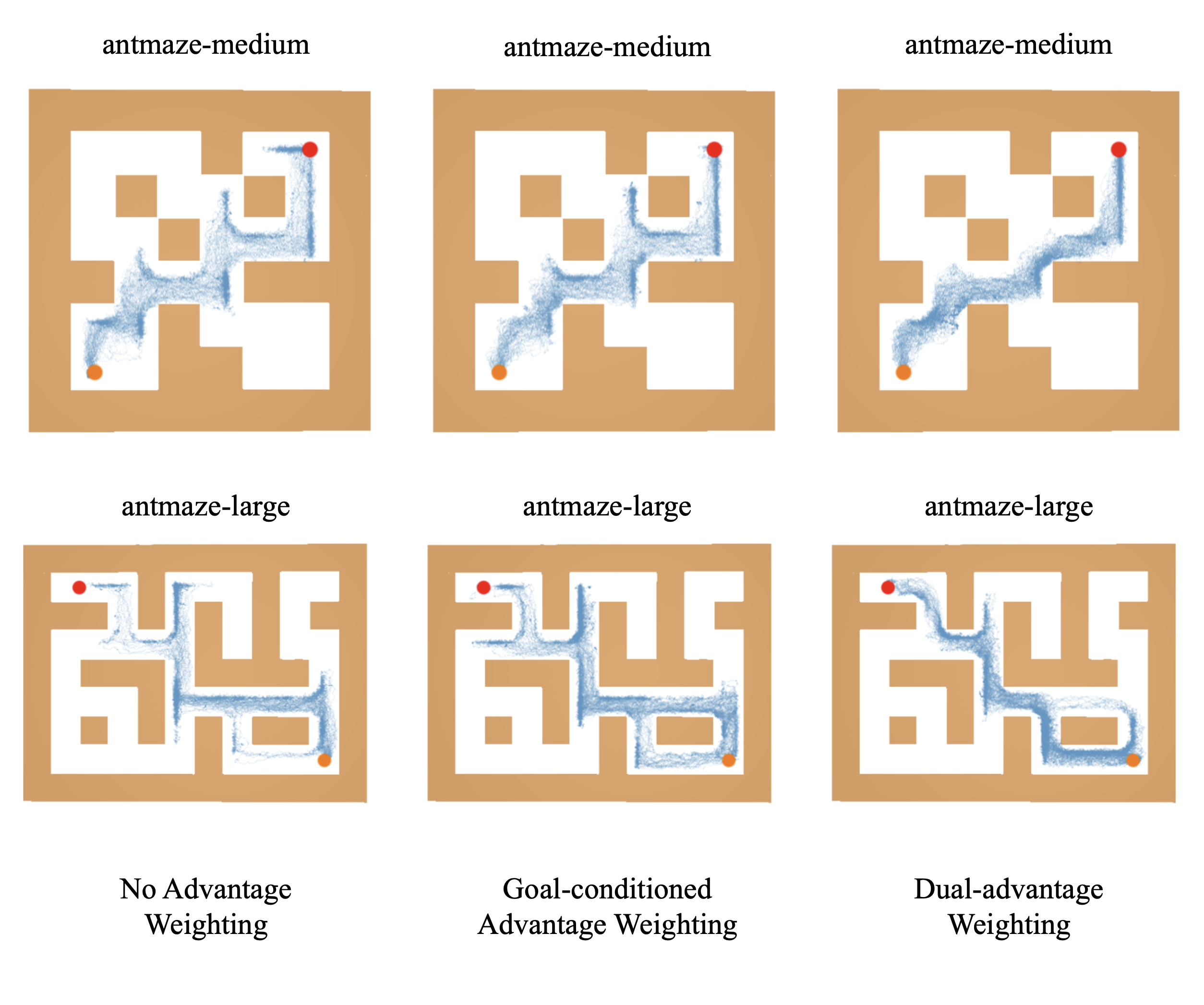
Figure 1: Visualisation of trajectories (in blue) in different maze environments. The trajectories have been generated by policies trained via supervised learning with different action weighting schemes: no action weighting (left), goal-conditioned advantage weighting (middle) and dual-advantage weighting (right). In this task, an agent (ant) needs to reach the end goal (red circle) from a starting position (orange circle). The proposed dual-advantage weighting scheme can remarkably alleviate the multi-modality issue.

In this study, we explore a complementary advantage-based action weighting scheme that further capitalizes on the goal-conditioned value function. During training, the state space is iteratively divided into a fixed number of regions, ensuring that all states within the same region have approximately the same goal-conditioned value. These regions are then ranked from the lowest to the highest value. Given the current state, the policy is encouraged to reach the immediately higher-ranking region, relative to the state’s present region, in the fewest steps possible. This ”target region” offers a state-dependent, short-horizon objective that is easier to achieve compared to the final goal, leading to generally shorter successful trajectories. Our proposed algorithm, Dual-Advantage Weighted Offline GCRL (DAWOG), seamlessly integrates the original goal-conditioned advantage weight with the new target-based advantage to effectively address the multi-modality issue.

A motivating example is illustrated in Figure 1, which presents the behavior of three pre-trained policies in maze-based navigation environments. A quadruped robot has learned to navigate through the maze. The robot is given previously unseen goals (red circles) that must be reached from a starting position (orange circles). The policies have been trained using supervised learning with no action weighting as a baseline (left), goal-conditioned advantage weighting (middle), and the proposed dual-advantage weighting (right). While goal-conditioned advantage weighting generally improves upon the baseline, the policy can sometimes lead the robot to sub-optimal regions, necessitating additional time steps before returning on track towards the goal. Remarkably, the proposed dual-advantage weighting scheme can alleviate the multi-modality issue and produce policies that take fewer detours, reaching the goal through smoother and shorter trajectories.

The main contributions of this paper are as follows. First, we introduce DAWOG, a simple-to-train and stable algorithm for offline GCRL. Second, we provide theoretical guarantees that DAWOG never performs worse than the underlying behavior policy. Third, we extensively evaluate DAWOG on benchmark datasets fu2020d4rl ; plappert2018multi ; yang2022rethinking in comparison with several competing offline learning algorithms, including methods adaptable for the goal-conditioned setting. Our empirical results demonstrate that DAWOG improves upon the current state-of-the-art performance, particularly in the AntMaze environments fu2020d4rl even in challenging settings where goals are uniformly sampled across the entire maze. Lastly, we present a series of additional studies to illustrate DAWOG’s properties and its low sensitivity to hyperparameters.

2 Related Work

In this section, we offer a brief overview of methodologically related approaches. In goal-conditioned RL (GCRL) In goal-conditioned RL (GCRL), one of the main challenges is the sparsity of the reward signal. An effective solution is hindsight experience replay (HER) andrychowicz2017hindsight , which relabels failed rollouts that have not been able to reach the original goals and treats them as successful examples for different goals thus effectively learning from failures. HER has been extended to solve different challenging tasks in synergy with other learning techniques, such as curriculum learning fang2019curriculum , model-based goal generation yang2021mher ; jurgenson2020sub ; nasiriany2019planning ; nair2018visual , and generative adversarial learning durugkar2021adversarial ; charlesworth2020plangan . In the offline setting, GCRL aims to learn goal-conditioned policies using only a fixed dataset. The simplest solution has been to adapt standard offline reinforcement learning algorithms kumar2020conservative ; fujimoto2021minimalist by simply concatenating the state and the goal as a new state. Chebotar et al. chebotar2021actionable propose goal-conditioned conservative Q-learning and goal-chaining to prevent value over-estimation and increase the diversity of the goal. Some of the previous works design offline GCRL algorithms from the perspective of state-occupancy matching eysenbach2022contrastive . Mezghani et al. mezghani2022learning propose a self-supervised reward shaping method to facilitate offline GCRL.

Our work is most related to goal-conditioned imitation learning (GCIL). Emmons et al. emmons2022rvs study the importance of concatenating goals with states showing its effectiveness in various environments. Ding et al. ding2019goal extend generative adversarial imitation learning ho2016generative to goal-conditioned settings. Ghosh et al. ghosh2021learning extend behaviour cloning bain1995framework to goal-conditioned settings and propose goal-conditioned supervised learning (GCSL) to imitate relabelled offline trajectories. Yang et al. yang2022rethinking connect GCSL to offline GCRL, and show that the objective function in GCSL is a lower bound of a function of the original GCRL objective. They propose the WGCSL algorithm, which re-weights the offline data based on advantage function similarly to peng19advantage ; wang2018exponentially . We addresses the offline GCRL problem using a similar approach, but extend the idea further by designing a new advantage-based action re-weighting scheme.

Some connections can also be found with goal-based hierarchical reinforcement learning methodsli2022hierarchical ; chane2021goal ; kim2021landmarkguided ; zhang2021worldmodel ; nasiriany2019planning . These works feature a high-level model capable of predicting a sequence of intermediate sub-goals and learn low-level policies to achieve them. Instead of learning to reach a specific sub-goals, our policy learns to reach an entire sub-region of the state space containing states that are equally valuable and provide an incremental improvement towards the final goal.

Lastly, there have been other applications of state space partitioning in reinforcement learning, such as facilitating exploration and accelerating policy learning in online settings ma2020clustered ; wei2018learning ; karimpanal2017identification ; mannor2004dynamic . Ghosh et al. ghosh2018divide demonstrate that learning a policy confined to a state partition instead of the whole space can lead to low-variance gradient estimates for learning value functions. In their work, states are partitioned using K-means to learn an ensemble of locally optimal policies, which are then progressively merged into a single, better-performing policy. Instead of partitioning states based on their geometric proximity, we partition states according to the proximity of their corresponding goal-conditioned values. We then use this information to define an auxiliary reward function and, consequently, a region-based advantage function.

3 Preliminaries

Goal-conditioned MDPs. Goal-conditioned tasks are usually modelled as Goal-Conditioned Markov Decision Processes (GCMDP), denoted by a tuple $<\mathcal{S},\mathcal{A},\mathcal{G},P,R>$ where $\mathcal{S}$, $\mathcal{A}$, and $\mathcal{G}$ are the state, action and goal space, respectively. For each state $s\in\mathcal{S}$, there is a corresponding achieved goal, $\phi(s)\in\mathcal{G}$, where $\phi:\mathcal{S}\rightarrow\mathcal{G}$ liu2022goal . At a given state $s_{t}$, an action $a_{t}$ taken towards a desired goal $g$ results in a visited next state $s_{t+1}$ according to the environment’s transition dynamics, $P(s_{t+1}\mid s_{t},a_{t})$. The environment then provides a reward, $r_{t}=R(s_{t+1},g)$, which is non-zero only when the goal has been reached, i.e.,

$$R(s,g)=\begin{cases}1,&\text{if $\mid\mid\phi(s)-g\mid\mid^{2}_{2}\leq\text{threshold}$,}\\ 0,&\text{otherwise.}\\ \end{cases}$$ (1)

Offline Goal-conditioned RL. In offline GCRL, the agent aims to learn a goal-conditioned policy, $\pi:\mathcal{S}\times\mathcal{G}\rightarrow\mathcal{A}$, using an offline dataset containing previously logged trajectories that might be generated by any number of unknown behaviour policies. The objective is to maximise the expected and discounted cumulative returns,

$$J_{GCRL}(\pi)=\mathbb{E}_{\begin{subarray}{c}g\sim P_{g},s_{0}\sim P_{0},\\ a_{t}\sim\pi(\cdot\mid s_{t},g),\\ s_{t+1}\sim P(\cdot\mid s_{t},a_{t})\end{subarray}}\left[\sum^{T}_{t=0}\gamma^{t}r_{t}\right],$$ (2)

where $\gamma\in(0,1]$ is a discount factor, $P_{g}$ is the distribution of the goals, $P_{0}$ is the distribution of the initial state, and $T$ corresponds to the time step at which an episode ends, i.e., either the goal has been achieved or timeout has been reached.

Goal-conditioned Supervised Learning (GCSL). GCSL ghosh2021learning relabels the desired goal in each data tuple $(s_{t},a_{t},g)$ with the goal achieved henceforth in the trajectory to increase the diversity and quality of the data andrychowicz2017hindsight ; kaelbling1993learning . The relabelled dataset is denoted as $\mathcal{D}_{R}=\{(s_{t},a_{t},g=\phi(s_{i}))\mid T\geq i>t\geq 0\}$. GCSL learns a policy that mimics the relabelled transitions by maximizing

$$J_{GCSL}(\pi)=\mathbb{E}_{(s_{t},a_{t},g)\sim\mathcal{D}_{R}}\left[\pi(a_{t}\mid s_{t},g)\right].$$ (3)

Yang et al. yang2022rethinking have connected GCSL to GCRL and demonstrated that $J_{GCSL}$ lower bounds $\frac{1}{T}\log J_{GCRL}$.

Goal-conditioned Value Functions. A goal-conditioned state-action value function schaul2015universal quantifies the value of an action $a$ taken from a state $s$ conditioned on a goal $g$ using the sparse rewards of Eq. 1,

$$Q^{\pi}(s,a,g)=\mathbb{E}_{\pi}\left[\sum^{T}_{t=0}\gamma^{t}r_{t}\mid s_{0}=s,a_{0}=a\right]$$ (4)

where $\mathbb{E}_{\pi}[\cdot]$ denotes the expectation taken with respect to $a_{t}\sim\pi(\cdot\mid s_{t},g)$ and $s_{t+1}\sim P(\cdot\mid s_{t},a_{t})$. Analogously, the goal-conditioned state value function quantifies the value of a state $s$ when trying to reach $g$,

$$V^{\pi}(s,g)=\mathbb{E}_{\pi}\left[\sum^{T}_{t=0}\gamma^{t}r_{t}\mid s_{0}=s\right].$$ (5)

The goal-conditioned advantage function,

$$A^{\pi}(s,a,g)=Q^{\pi}(s,a,g)-V^{\pi}(s,g),$$ (6)

then quantifies how advantageous it is to take a specific action $a$ in state $s$ towards $g$ over taking the actions sampled from $\pi(\cdot\mid s,g)$ yang2022rethinking .

4 Methods

In this section, we formally present the proposed methodology and analytical results. First, we introduce a notion of target region advantage function in Section 4.1, which we use to develop the learning algorithm in Section 4.2. In Section 4.3 we provide a theoretical analysis offering guarantees that DAWOG learns a policy that is never worse than the underlying behaviour policy.

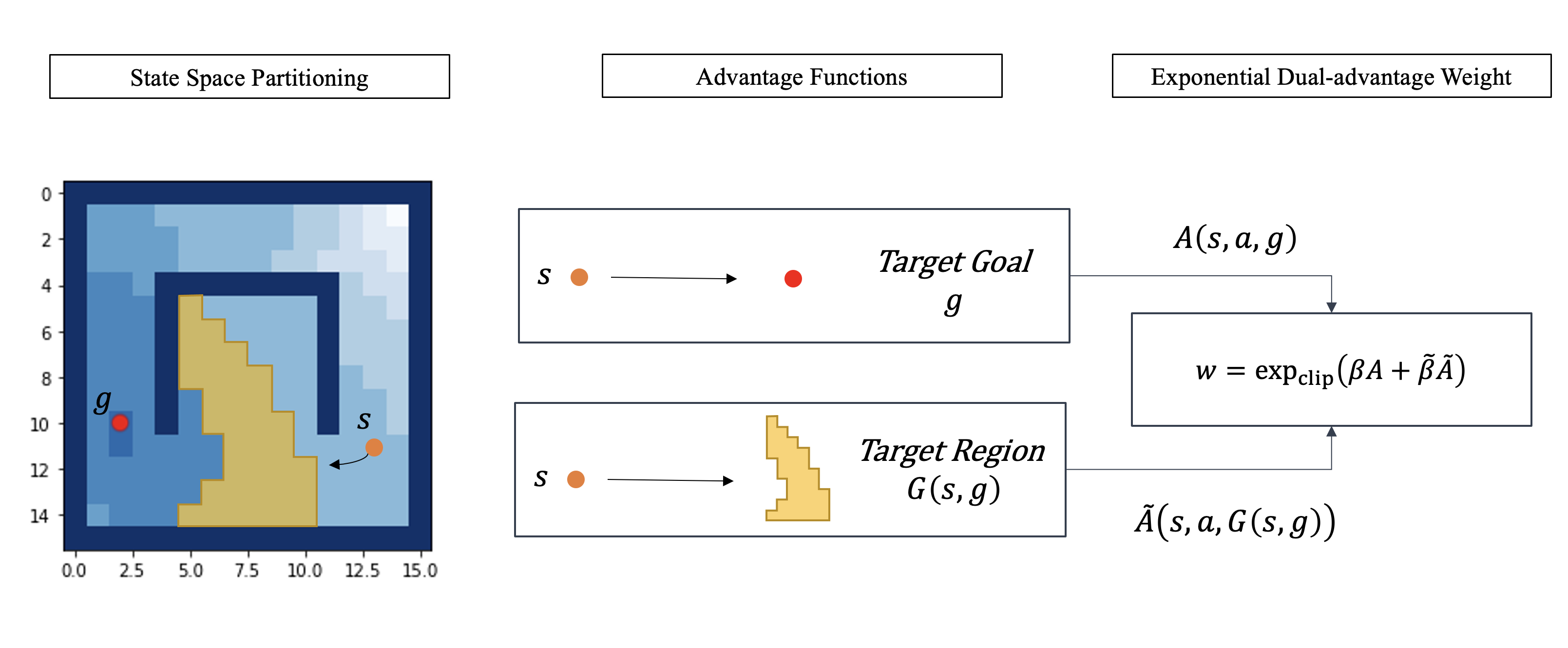
Figure 2: Illustration of the two advantage functions used by DAWOG for a simple navigation task. First, a goal-conditioned advantage is learnt using only relabelled offline data. Then, a target-region advantage is obtained by partitioning the states according to their goal-conditioned value function, identifying a target region, and rewarding actions leading to this region in the smallest possible number of steps. DAWOG updates the policy to imitate the offline data through an exponential weighting factor that depends on both advantages.

4.1 Target region advantage function

For any state $s\in\mathcal{S}$ and goal $g\in\mathcal{G}$, the domain of the goal-conditioned value function in Eq. 5 is the unit interval due to the binary nature of the reward function in Eq. 1. Given a positive integer $K$, we partition $[0,1]$ into $K$ equally sized intervals, $\{\beta_{i}\}_{i=1,\ldots,K}$. For any goal $g$, this partition induces a corresponding partition of the state space.

Definition 1.

(Goal-conditioned State Space Partition) For a fixed desired goal $g\in\mathcal{G}$, the state space is partitioned into $K$ equally sized regions according to $V^{\pi}(\cdot,g)$. The $k^{th}$ region, notated as $B_{k}(g)$, contains all states whose goal-conditioned values are within $\beta_{k}$, i.e.,

$$B_{k}(g)=\{s\in\mathcal{S}\mid V^{\pi}(s,g)\in\beta_{k}\}.$$ (7)

Our ultimate objective is to up-weight actions taken in a state $s_{t}\in B_{k}(g)$ that are likely to lead to a region only marginally better (but never worse) than $B_{k}(g)$ as rapidly as possible.

Definition 2.

(Target Region) For $s\in B_{k}(g)$, the mapping $b(s,g):\mathcal{S}\times\mathcal{G}\rightarrow\{1,\ldots,K\}$ returns the correct index $k$. The goal-conditioned target region is defined as

$$G(s,g)=B_{\min\{b(s,g)+1,K\}}(g),$$ (8)

which is the set of states whose goal-conditioned value is not less than the states in the current region. For $s\in B_{k}(g)$, $G(s,g)$ is the current region $B_{k}(g)$ if and only if $k=K$.

We now introduce two target region value functions.

Definition 3.

(Target Region Value Functions) For a state $s$, action $a\in\mathcal{A}$, and the target region $G(s,g)$, we define a target region V-function and a target region Q-function based on an auxiliary reward function that returns a non-zero reward only when the next state belongs to the target region, i.e.,

$$\tilde{r}_{t}=\tilde{R}(s_{t},s_{t+1},G(s_{t},g))=\begin{cases}1,&\text{if }s_{t+1}\in G(s_{t},g)\\ 0,&\text{otherwise.}\\ \end{cases}$$ (9)

The target region Q-value function is

$$\tilde{Q}^{\pi}(s,a,G(s,g))=\mathbb{E}_{\pi}\left[\sum^{\tilde{T}}_{t=0}\gamma^{t}\tilde{r}_{t}\mid s_{0}=s,a_{0}=a\right],$$ (10)

where $\tilde{T}$ corresponds to the time step at which the target region is achieved or timeout is reached, $\mathbb{E}_{\pi}[\cdot]$ denotes the expectation taken with respect to the policy $a_{t}\sim\pi(\cdot\mid s_{t},g)$ and the transition dynamics $s_{t+1}\sim P(\cdot\mid s_{t},a_{t})$. The target region Q-function estimates the expected cumulative return when starting in $s_{t}$, taking an action $a_{t}$, and then following the policy $\pi$, based on the auxiliary reward. The discount factor $\gamma$ reduces the contribution of delayed target achievements. Analogously, the target region value function is defined as

$$\tilde{V}^{\pi}(s,G(s,g))=\mathbb{E}_{\pi}\left[\sum^{\tilde{T}}_{t=0}\gamma^{t}\tilde{r}_{t}\mid s_{0}=s\right]$$ (11)

and quantifies the quality of a state $s$ according to the same criterion.

Using the above value functions, we are in a position to introduce the corresponding target region advantage function.

Definition 4.

(Target Region Advantage Function) The target region-based advantage function is defined as

$$\tilde{A}^{\pi}(s,a,G(s,g))=\tilde{Q}^{\pi}(s,a,G(s,g))-\tilde{V}^{\pi}(s,G(s,g)).$$ (12)

It estimates the advantage of action $a$ towards the target region in terms of the cumulative return by taking $a$ in state $s$ and following the policy $\pi$ thereafter, compared to taking actions sampled from the policy.

4.2 The DAWOG algorithm

The proposed DAWOG belongs to the family of WGCSL algorithms, i.e. it is designed to optimise the following objective function

$$J_{DAWOG}(\pi)=\mathbb{E}_{(s_{t},a_{t},g)\sim\mathcal{D}_{R}}\left[w_{t}\log\pi(a_{t}\mid s_{t},g)\right]$$ (13)

where the role of $w_{t}$ is to re-weight each action’s contribution to the loss. In DAWOG, $w_{t}$ is an exponential weight of form

$$w_{t}=\exp_{clip}(\beta A^{\pi_{b}}(s_{t},a_{t},g)+\tilde{\beta}\tilde{A}^{\pi_{b}}(s_{t},a_{t},G(s_{t},g)),$$ (14)

where $\pi_{b}$ is the underlying behaviour policy that generate the relabelled dataset $\mathcal{D}_{R}$. The contribution of the two advantage functions, $\tilde{A}^{\pi_{b}}(s_{t},a_{t},g)$ and $\tilde{A}^{\pi_{b}}(s_{t},a_{t},G(s_{t},g))$, is controlled by positive scalars, $\beta$ and $\tilde{\beta}$, respectively. However, empirically, we have found that using a single shared parameter generally performs well across the tasks we have considered (see Section 5.5). The clipped exponential, $\exp_{clip}(\cdot)$, is used for numerical stability and keeps the values within the $(0,M]$ range, for a given $M>0$ threshold.

The algorithm combines the originally proposed goal-conditioned advantage yang2022rethinking with the novel target region advantage. The former ensures that actions likely to lead to the goal are up-weighted. However, when the goal is still far, there may still be several possible ways to reach it, resulting in a wide variety of favourable actions. The target region advantage function provides additional guidance by further increasing the contribution of actions expected to lead to a higher-valued sub-region of the state space as rapidly as possible. Both $A^{\pi_{b}}(s_{t},a_{t},g)$ and $\tilde{A}^{\pi_{b}}(s_{t},a_{t},G(s_{t},g))$ are beneficial in a complementary fashion: whereas the former is more concerned with long-term gains, which are more difficult and uncertain, the latter is more concerned with short-term gains, which are easier to achieve. As such, these two factors are complementary and their combined effect plays an important role in the algorithm’s final performance (see Section 5.5). An illustration of the dual-advantage weighting scheme is shown in Fig.2.

In the remainder, we explain the entire training procedure. The advantage $A^{\pi_{b}}(s_{t},a_{t},g)$ is estimated via

$$A^{\pi_{b}}(s_{t},a_{t},g)=r_{t}+\gamma V^{\pi_{b}}(s_{t+1},g)-V^{\pi_{b}}(s_{t},g).$$ (15)

In practice, the goal-conditioned V-function is approximated by a deep neural network with parameter $\psi_{1}$, which is learnt by minimising the temporal difference (TD) error sutton2018reinforcement :

$$\mathcal{L}(\psi_{1})=\mathbb{E}_{(s_{t},s_{t+1},g)\sim\mathcal{D}_{R}}\left[(V_{\psi_{1}}(s_{t},g)-y_{t})^{2}\right],$$ (16)

where $y_{t}$ is the target value given by

$$y_{t}=r_{t}+\gamma(1-d(s_{t+1},g))V_{\psi^{-}_{1}}(s_{t+1},g).$$ (17)

Here $d(s_{t+1},g)$) indicates whether the state $s_{t+1}$ has reached the goal $g$. The parameter vector $\psi^{-}_{1}$ is a slowly moving average of $\psi_{1}$ to stabilise training mnih2015human . Analogously, the target region advantage function is estimated by

$$\tilde{A}^{\pi_{b}}(s_{t},a_{t},G(s_{t},g))=\tilde{r}_{t}+\gamma\tilde{V}^{\pi_{b}}(s_{t+1},G(s_{t},g))-\tilde{V}^{\pi_{b}}(s_{t},G(s_{t},g)),$$ (18)

where the target region V-function is approximated with a deep neural network parameterised with $\psi_{2}$. The relevant loss function is

$$\mathcal{L}(\psi_{2})=\mathbb{E}_{(s_{t},s_{t+1},g)\sim\mathcal{D}_{R}}\left[(\tilde{V}_{\psi_{2}}(s_{t},G(s_{t},g))-\tilde{y}_{t})^{2}\right],$$ (19)

where the target value is

$$\tilde{y}_{t}=\tilde{r}_{t}+\gamma(1-\tilde{d}(s_{t+1},G(s_{t},g)))\tilde{V}_{\psi^{-}_{2}}(s_{t+1},G(s_{t},g)).$$ (20)

and $\tilde{d}(s_{t+1},G(s_{t},g))$) indicates whether the state $s_{t+1}$ has reached the target region $G(s_{t},g)$. $\psi^{-}_{2}$ is a slowly moving average of $\psi_{2}$. The full procedure is presented in Algorithm 1 where the two value functions are jointly optimised and contribute to optimising Eq. 13.

Algorithm 1 Dual-Advantage Weighted Offline GCRL (DAWOG)

1:parameters $\theta$, $\psi_{1}$, $\psi^{-}_{1}$, $\psi_{2}$, and $\psi^{-}_{2}$ for policy network, goal-conditioned value network and its target network, partition-conditioned value network and its target network, respectively; relabelled dataset $\mathcal{D}_{R}$

2:while not converged do

3:     for $i=1,\ldots,I$ do

4:         Sample a minibatch $\{(s,a,s^{\prime},g)\}^{B}_{b=1}$ from $D_{R}$.

5:         Update $\psi_{1}$ to minimise Eq. 16.

6:         Update $\psi_{2}$ to minimise Eq. 19.

7:         Comp. $A(s,a,g)=r_{t}+\gamma V_{\psi_{1}}(s^{\prime},g)-V_{\psi_{2}}(s,g)$.

8:         Comp. $\tilde{A}(s,a,G(s,g))=\tilde{r}_{t}+\gamma\tilde{V}_{\psi_{2}}(s^{\prime},G(s,g))-\tilde{V}_{\psi_{2}}(s,G(s,g))$.

9:         Update the policy by minimising Eq. 13.

10:     end for

11:     $\psi^{-}_{1}\leftarrow\rho\psi_{1}+(1-\rho)\psi^{-}_{1}$.

12:     $\psi^{-}_{2}\leftarrow\rho\psi_{2}+(1-\rho)\psi^{-}_{2}$.

13:end while

14:return $\pi_{\theta}$.

4.3 Policy improvement guarantees

In this section, we demonstrate that our learnt policy is never worse than the underlying behaviour policy $\pi_{b}$ that generates the relabelled data. First, we express the policy learnt by our algorithm in an equivalent form, as follows.

Proposition 1.

DAWOG learns a policy $\pi_{\theta}$ to minimise the KL-divergence from

$$\tilde{\pi}_{dual}(a\mid s,g)=\exp(w+N(s,g))\pi_{b}(a\mid s,g),$$ (21)

where $w=\beta A^{\pi_{b}}(s,a,g)+\tilde{\beta}\tilde{A}^{\pi_{b}}(s,a,G(s,g))$, $G(s,g)$ is the target region, and $N(s,g)$ is a normalising factor to ensuring that $\sum_{a\in\mathcal{A}}\tilde{\pi}_{dual}(a\mid s,g)=1$.

Proof: According to Eq. 13, DAWOG maximises the following objective with the policy parameterised by $\theta$:

$$\begin{split}\arg\max_{\theta}J(\theta)=&\arg\max_{\theta}\mathbb{E}_{(s,a,g)\sim\mathcal{D}_{R}}\left[\exp(w+N(s,g))\log\pi_{\theta}(a\mid s,g)\right]\\ =&\arg\max_{\theta}\mathbb{E}_{(s,g)\sim\mathcal{D}_{R}}\left[\sum_{a}\exp(w+N(s,g))\pi_{b}(a\mid s,g)\log\pi_{\theta}(a\mid s,g)\right]\\ =&\arg\max_{\theta}\mathbb{E}_{(s,g)\sim\mathcal{D}_{R}}\left[\sum_{a}\tilde{\pi}_{dual}(a\mid s,g)\log\pi_{\theta}(a\mid s,g)\right]\\ =&\arg\max_{\theta}\mathbb{E}_{(s,g)\sim\mathcal{D}_{R}}\left[\sum_{a}\tilde{\pi}_{dual}(a\mid s,g)\log\frac{\pi_{\theta}(a\mid s,g)}{\tilde{\pi}_{dual}(a\mid s,g)}\right]\\ =&\arg\min_{\theta}\mathbb{E}_{(s,g)\sim\mathcal{D}_{R}}\left[D_{KL}(\tilde{\pi}_{dual}(\cdot\mid s,g)\mid\mid\pi_{\theta}(\cdot\mid s,g))\right]\end{split}$$ (22)

$J(\theta)$ reaches its maximum when

$$D_{KL}(\tilde{\pi}_{dual}(\cdot\mid s,g)\mid\mid\pi_{\theta}(\cdot\mid s,g))=0,\forall s\in\mathcal{S},g\in\mathcal{G}.$$ (23)

Then, we propose Proposition 2 to show the condition for policy improvement.

Proposition 2.

wang2018exponentially ; yang2022rethinking Suppose two policies $\pi_{1}$ and $\pi_{2}$ satisfy

$$h_{1}(\pi_{2}(a\mid s,g))=h_{1}(\pi_{1}(a\mid s,g))+h_{2}(s,g,A^{\pi_{1}}(s,a,g))$$ (24)

where $h_{1}(\cdot)$ is a monotonically increasing function, and $h_{2}(s,g,\cdot)$ is monotonically increasing for any fixed $s$ and $g$. Then we have

$$V^{\pi_{2}}(s,g)\geq V^{\pi_{1}}(s,g),\forall s\in\mathcal{S}\text{ and }g\in\mathcal{G}.$$

That is, $\pi_{2}$ is uniformly as good as or better than $\pi_{1}$.

We want to leverage this result to demonstrate that $V^{\tilde{\pi}_{dual}}(s,g)\geq V^{\pi_{b}}(s,g)$ for any state $s$ and goal $g$. Firstly, we need to obtain a monotonically increasing function $h_{1}(\cdot)$. This is achieved by taking the logarithm of the both sides of Eq. 21, i.e.,

$$\begin{split}\log\tilde{\pi}_{dual}(a\mid s,g)=&\log\pi_{b}(a\mid s,g)+\beta A^{\pi_{b}}(s,a,g)\\ &+\tilde{\beta}\tilde{A}^{\pi_{b}}(s,a,G(s,g))+N(s,g).\end{split}$$ (25)

so that $h_{1}(\cdot)=\log(\cdot)$. The following proposition establishes that we also have a function $h_{2}(s,g,A^{\pi_{b}}(s,a,g))=\beta A^{\pi_{b}}(s,a,g)+\tilde{\beta}\tilde{A}^{\pi_{b}}(s,a,G(s,g))+N(s,g)$, which is monotonically increasing for any fixed $s$ and $g$. Since $\beta,\tilde{\beta}\geq 0$ and $N(s,g)$ is independent of the action, it is equivalent to prove that for any fixed $s$ and $g$, there exists a monotonically increasing function $l$ satisfying

$$l(s,g,\tilde{A}^{\pi_{b}}(s,a,G(s,g)))=A^{{\pi_{b}}}(s,a,g).$$ (26)

Proposition 3.

Given fixed $s$, $g$ and the target region $G(s,g)$, the goal-conditioned advantage function $A^{\pi}$ and the target region-conditioned advantage function $\tilde{A}^{\pi}$ satisfy $l(s,g,A^{\pi}(s,a,g))=\tilde{A}^{\pi}(s,a,G(s,g))$, where $l(s,g,\cdot)$ is monotonically increasing for any fixed $s$ and $g$.

Proof: By the definition of monotonically increasing function, if for all $a^{\prime},a^{\prime\prime}\in\mathcal{A}$ such that $A^{\pi}(s,a^{\prime},g)\geq A^{\pi}(s,a^{\prime\prime},g)$ and we can reach $\tilde{A}^{\pi}(s,a^{\prime},G(s,g))\geq\tilde{A}^{\pi}(s,a^{\prime\prime},G(s,g))$, then the proposition can be proved.

We start by having any two actions $a^{\prime},a^{\prime\prime}\in\mathcal{A}$ such that

$$A^{\pi}(s,a^{\prime},g)\geq A^{\pi}(s,a^{\prime\prime},g).$$ (27)

By adding $V^{\pi}(s,g)$ on both sides, the inequality becomes

$$Q^{\pi}(s,a^{\prime},g)\geq Q^{\pi}(s,a^{\prime\prime},g).$$ (28)

By Definition 4, the goal-conditioned Q-function can be written as

$$Q^{\pi}(s,a,g)=\mathbb{E}_{\pi}\left[R_{t,\tau_{i}}\mid s_{t}=s,a_{t}=a\right],$$ (29)

where $\tau_{i}$ represents a trajectory: $s_{t},a_{t},r_{t}^{i},s_{t+1}^{i},a_{t+1}^{i},r_{t+1}^{i},\ldots,s_{T}^{i}$

$$R_{t,\tau_{i}}=r_{t}^{i}+\gamma r_{t+1}^{i}+\ldots+\gamma^{t_{tar}^{i}}V(s_{tar}^{i},g),$$ (30)

$s_{tar}^{i}$ corresponds to the state where $\tau_{i}$ gets into the target region, $t_{tar}^{i}$ is the corresponding time step. Because the reward is zero until the desired goal is reached, Eq. 29 can be written as

$$Q^{\pi}(s,a,g)=\mathbb{E}_{\pi}\left[\gamma^{t_{tar}^{i}}V(s_{tar}^{i},g)\mid s_{t}=s,a_{t}=a\right].$$ (31)

Similarly,

$$\tilde{Q}^{\pi}(s,a,G(s,g)) =\mathbb{E}_{\pi}\left[\gamma^{t_{tar}^{i}}\tilde{V}(s_{tar}^{i},G(s,g))\mid s_{t}=s,a_{t}=a\right]$$ (32)

$$=\mathbb{E}_{\pi}\left[\gamma^{t_{tar}^{i}}\mid s_{t}=s,a_{t}=a\right].$$

According to Eq.28 and Eq.31, we have

$$\mathbb{E}_{\pi}\left[\gamma^{t_{tar}^{i^{\prime}}}V(s_{tar}^{i^{\prime}},g)\mid s_{t}=s,a_{t}=a^{\prime}\right]\geq\mathbb{E}_{\pi}\left[\gamma^{t_{tar}^{i^{\prime\prime}}}V(s_{tar}^{i^{\prime\prime}},g)\mid s_{t}=s,a_{t}=a^{\prime\prime}\right].$$ (33)

Given the valued-based partitioning of the state space, we assume that the goal-conditioned values of states in the target region are sufficiently close such that $\forall i^{\prime},i^{\prime\prime},V(s_{tar}^{i^{\prime}},g)\approx v,V(s_{tar}^{i^{\prime\prime}},g)\approx v$. Then, Eq.33 can be approximated as

$$v\cdot\mathbb{E}_{\pi}\left[\gamma^{t_{tar}^{i^{\prime}}}\mid s_{t}=s,a_{t}=a^{\prime}\right]\geq v\cdot\mathbb{E}_{\pi}\left[\gamma^{t_{tar}^{i^{\prime\prime}}}\mid s_{t}=s,a_{t}=a^{\prime\prime}\right].$$ (34)

Removing $v$ on both sides of Eq.34 and according to Eq.32, we have

$$\tilde{Q}^{\pi}(s,a^{\prime},G(s,g))\geq\tilde{Q}^{\pi}(s,a^{\prime\prime},G(s,g)).$$ (35)

Then,

$$\tilde{A}^{\pi}(s,a^{\prime},G(s,g))\geq\tilde{A}^{\pi}(s,a^{\prime\prime},G(s,g)).$$ (36)

5 Experimental results

In this section, we examine DAWOG’s performance relative to existing state-of-the-art algorithms using environments of increasing complexity. The remainder of this section is organized as follows. The benchmark tasks and datasets are presented in Section 5.1. The implementation details are provided in Section 5.2. A list of competing methods is presented in Section 5.3, and the comparative performance results are found in Section 5.4. Here, we also qualitatively inspect the policies learnt by DAWOG in an attempt to characterise the improvements that can be achieved over other methods. Section 5.5 presents extensive ablation studies to appreciate the relative contribution of the different advantage weighting factors. Finally, in Section 5.6, we study how the dual-advantage weight depends on its hyperparameters.

5.1 Tasks and datasets

5.1.1 Grid World

We designed two $16\times 16$ grid worlds to assess the performance on a simple navigation task. From its starting position on the grid, an agent needs to reach a goal that has been randomly placed in one of the available cells. Only four actions are available to move left, right, up, and down. The agent accrues a positive reward when it reaches the cell containing the goal. To generate the benchmark dataset, we trained a Deep Q-learning algorithm mnih2015human , whose replay buffer, containing $4,000$ trajectories of $50$ time steps, was used as the benchmark dataset.

5.1.2 AntMaze Navigation

The AntMaze suite used in our experiment is obtained from the D4RL benchmark fu2020d4rl , which has been widely adopted by offline GCRL studies eysenbach2022contrastive ; emmons2022rvs ; li2022hierarchical . The task requires to control an 8-DoF quadruped robot that moves in a maze and aims to reach a target location within an allowed maximum of $1,000$ steps. The suite contains three kinds of different maze layouts: umaze (a U-shape wall in the middle), medium and large, and provides three training datasets. The datasets differ in the way the starting and goal positions of each trajectory were generated: in umaze the starting position is fixed and the goal position is sampled within a fixed-position small region; in diverse the starting and goal positions are randomly sampled in the whole environment; finally, in play, the starting and goal positions are randomly sampled within hand-picked regions. In the sparse-reward environment, the agent obtains a reward only when it reaches the target goal. We use a normalised score as originally proposed in fu2020d4rl , i.e.,

$$s_{n}=100\cdot\frac{s-s_{r}}{s_{e}-s_{r}}$$

where $s$ is the unnormalised score, $s_{r}$ is a score obtained using a random policy and $s_{e}$ is the score obtained using an expert policy.

In our evaluation phase, the policy is tested online. The agent’s starting position is always fixed, and the goal position is generated using one of the following methods:

• fixed goal: the goal position is sampled within a small and fixed region in a corner of the maze, as in previous work eysenbach2022contrastive ; emmons2022rvs ; li2022hierarchical ;

• diverse goal: the goal position is uniformly sampled over the entire region. This evaluation scheme has not been adopted in previous works, but helps assess the policy’s generalisation ability in goal-conditioned settings.

5.1.3 Gym Robotics

Gym Robotics plappert2018multi is a popular robotic suite used in both online and offline GCRL studies yang2022rethinking ; eysenbach2022contrastive . The agent to be controlled is a 7-DoF robotic arm, and several tasks are available: in FetchReach, the arm needs to touch a desired location; in FetchPush, the arm needs to move a cube to a desired location; in FetchPickAndPlace a cube needs to be picked up and moved to a desired location; finally, in FetchSlide, the arm needs to slide a cube to a desired location. Each environment returns a reward of one when the task has been completed within an allowed time horizon of $50$ time steps. For this suite, we use the expert offline dataset provided by yang2022rethinking . The dataset for FetchReach contains $1\times 10^{5}$ time steps whereas all the other datasets contain $2\times 10^{6}$ steps. The datasets are collected using a pre-trained policy using DDPG and hindsight relabelling lillicrap2016continuous ; andrychowicz2017hindsight ; the actions from the policy were perturbed by adding Gaussian noise with zero mean and $0.2$ standard deviation.

5.2 Implementation details

DAWOG’s training procedure is shown in Algorithm 1. In our implementation, for continuous control tasks, we use a Gaussian policy following previous recommendations raffin2021stablebaselines . When interacting with the environment, the actions are sampled from the above distribution. All the neural networks used in DAWOG are 3-layer multi-layer perceptrons with $512$ units in each layer and ReLU activation functions. The parameters are trained using the Adam optimiser kingma2014adam with a learning rate $1\times 10^{-3}$. The training batch size is $512$ across all networks. To represent $G(s,g)$ we use a $K$-dimensional one-hot encoding vector where the $i^{th}$ position is non-zero for the target region and zero everywhere else along with the goal $g$. Four hyper-parameters need to be chosen: the state partition size, $K$, the two coefficients controlling the relative contribution of the two advantage functions, $\beta$ and $\tilde{\beta}$, and the clipping bound, $M$. In our experiments, we use $K=20$ for umaze and medium maze, $K=50$ for large maze, and $K=10$ for all other tasks. In all our experiments, we use fixed values of $\beta=\tilde{\beta}=10$. The clipping bound is always kept at $M=10$.

5.3 Competing methods

Several competing algorithms have been selected for comparison with DAWOG, including offline DRL methods that were not originally proposed for goal-conditioned tasks and required some minor adaptation. In the remainder of this Section, the nomenclature ’g-’ indicates that the original algorithm has been implemented to operate in a goal-conditioned setting by concatenating the state and the goal as a new state and with hindsight relabelling.

The first category of algorithms includes regression-based methods that imitate the relabelled offline dataset using different weighting strategies:

• GCSL ghosh2021learning imitates the relabelled transitions without any weighting strategies;

• g-MARWILwang2018exponentially incorporates goal-conditioned advantage to weight the actions’ contribution in the offline data;

• WGCSL yang2022rethinking incorporates goal-conditioned advantage to weight the actions’ contribution using multiple criteria.

We also include three actor-critic methods:

• Contrastive RL eysenbach2022contrastive estimates a Q-function by contrastive learning;

• g-CQL kumar2020conservative learns a conservative Q-function;

• g-BCQ fujimoto2019off learns a Q-function by clipped double Q-learning with a restricted policy;

• g-TD3-BC fujimoto2021minimalist combines TD3 algorithm fujimoto2018addressing with a behavior cloning regularizer.

Finally, we include a hierarchical learning method, IRIS mandlekar2020iris , which employs a low-level imitation learning policy to reach sub-goals commanded by a high-level goal planner.

5.4 Performance comparisons and analysis

Table 1: Experiment results for the two Grid World navigation environments.

Environment	DAWOG	GCSL	g-MAR.
grid-wall	$\textbf{87.2}_{\pm 1.9}$	$70.6_{\pm 4.8}$	$79.8_{\pm 4.0}$
grid-umaze	$\textbf{82.4}_{\pm 2.6}$	$68.0_{\pm 3.8}$	$77.2_{\pm 3.5}$

Table 2: Experiment results in Gym Robotics.

Environment	DAWOG	GCSL	WGCSL	g-MAR.	CRL	g-CQL	g-TD3.	g-BCQ
FetchReach	$\textbf{46.7}_{\pm 0.1}$	$41.7_{\pm 0.3}$	$46.3_{\pm 0.1}$	$45.0_{\pm 0.1}$	$46.1_{\pm 0.1}$	$1.0_{\pm 0.2}$	$45.5_{\pm 0.3}$	$35.1_{\pm 3.1}$
FetchPush	$\textbf{39.3}_{\pm 0.2}$	$28.5_{\pm 0.9}$	$39.1_{\pm 0.2}$	$37.4_{\pm 0.2}$	$36.5_{\pm 0.6}$	$5.7_{\pm 0.8}$	$30.8_{\pm 0.6}$	$3.6_{\pm 0.9}$
FetchPickAndPlace	$\textbf{37.9}_{\pm 0.4}$	$25.2_{\pm 0.8}$	$34.3_{\pm 0.5}$	$34.5_{\pm 0.5}$	$35.7_{\pm 0.2}$	$3.2_{\pm 2.5}$	$36.5_{\pm 0.5}$	$1.4_{\pm 0.2}$
FetchSlide	$9.9_{\pm 0.8}$	$3.05_{\pm 0.6}$	$\textbf{10.7}_{\pm 1.0}$	$4.5_{\pm 1.7}$	$9.9_{\pm 0.2}$	$0.8_{\pm 0.3}$	$5.8_{\pm 0.6}$	$0.1_{\pm 0.1}$

Table 3: Experiment results in AntMaze environments. The results are normalised by the expert score from D4RL paper.

	Environment	DAWOG	GCSL	WGCSL	g-MAR.	CRL	g-CQL	g-TD3.	IRIS
	umaze	$\textbf{92.8}_{\pm 3.3}$	$64.4_{\pm 5.0}$	$85.8_{\pm 2.9}$	$83.2_{\pm 5.0}$	$81.9_{\pm 1.7}$	$66.0_{\pm 2.6}$	$83.2_{\pm 9.6}$	$82.6_{\pm 4.7}$
	umaze-diverse	$\textbf{90.4}_{\pm 3.3}$	$65.4_{\pm 3.7}$	$81.6_{\pm 7.8}$	$70.4_{\pm 5.6}$	$75.4_{\pm 3.5}$	$58.4_{\pm 2.4}$	$77.8_{\pm 8.8}$	$89.4_{\pm 2.4}$
Fixed Goal	medium-play	$\textbf{86.6}_{\pm 6.4}$	$61.8_{\pm 9.2}$	$50.4_{\pm 7.0}$	$64.4_{\pm 5.2}$	$71.5_{\pm 5.2}$	$27.0_{\pm 4.5}$	$66.0_{\pm 8.0}$	$73.1_{\pm 4.5}$
	medium-diverse	$\textbf{87.4}_{\pm 5.7}$	$64.2_{\pm 3.7}$	$46.4_{\pm 6.9}$	$63.0_{\pm 7.8}$	$72.5_{\pm 2.8}$	$32.4_{\pm 4.1}$	$52.6_{\pm 9.2}$	$64.8_{\pm 2.6}$
	large-play	$\textbf{58.6}_{\pm 6.2}$	$30.6_{\pm 7.6}$	$30.4_{\pm 6.2}$	$20.4_{\pm 5.8}$	$41.6_{\pm 6.0}$	$8.6_{\pm 4.2}$	$30.6_{\pm 6.0}$	$57.9_{\pm 3.6}$
	large-diverse	$\textbf{52.0}_{\pm 8.6}$	$32.6_{\pm 8.5}$	$29.8_{\pm 5.8}$	$25.2_{\pm 6.7}$	$49.3_{\pm 6.3}$	$8.8_{\pm 3.6}$	$39.8_{\pm 8.9}$	$43.7_{\pm 1.3}$
	umaze	$\textbf{75.6}_{\pm 5.1}$	$61.2_{\pm 3.1}$	$74.4_{\pm 7.5}$	$67.4_{\pm 3.0}$	$60.4_{\pm 3.2}$	$58.3_{\pm 2.5}$	$63.0_{\pm 5.5}$	-—
	umaze-diverse	$\textbf{75.2}_{\pm 4.6}$	$58.2_{\pm 5.1}$	$74.0_{\pm 6.3}$	$60.2_{\pm 3.6}$	$49.6_{\pm 4.6}$	$54.6_{\pm 5.2}$	$54.8_{\pm 2.5}$	-—
Diverse Goal	medium-play	$\textbf{70.6}_{\pm 2.6}$	$45.4_{\pm 5.4}$	$39.2_{\pm 5.2}$	$43.6_{\pm 6.6}$	$26.6_{\pm 2.4}$	$33.6_{\pm 2.6}$	$38.0_{\pm 2.4}$	-—
	medium-diverse	$\textbf{72.8}_{\pm 3.1}$	$43.2_{\pm 4.3}$	$38.4_{\pm 5.7}$	$49.6_{\pm 5.4}$	$28.6_{\pm 2.8}$	$34.4_{\pm 2.0}$	$45.6_{\pm 5.2}$	-—
	large-play	$\textbf{44.2}_{\pm 4.3}$	$35.0_{\pm 6.4}$	$31.4_{\pm 2.4}$	$41.2_{\pm 2.5}$	$24.6_{\pm 5.3}$	$18.3_{\pm 7.5}$	$31.4_{\pm 3.2}$	-—
	large-diverse	$\textbf{43.8}_{\pm 4.6}$	$35.4_{\pm 2.8}$	$28.3_{\pm 2.8}$	$40.4_{\pm 5.6}$	$26.0_{\pm 2.4}$	$24.6_{\pm 4.1}$	$33.6_{\pm 5.9}$	-—

To appreciate how state space partitioning works, we provide examples of valued-based partition for the grid worlds environments in Figure 3. In these cases, the enviromental states simply correspond to locations in the grid. Here, the state space is divided with darker colours indicating higher values. As expected, these figures clearly show that states can be ordered based on the estimated value function, and that higher-valued states are those close to the goal. We also report the average return across five runs in Table 1 where we compare DAWOG against GCSL and g-MAR. - two algorithms that are easily adapted for discrete action spaces.

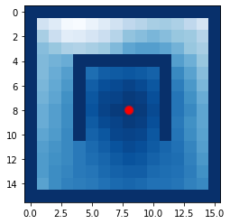
(a)

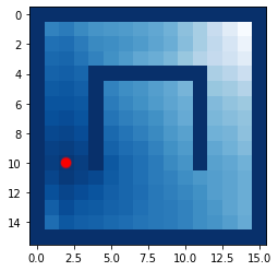
(b)

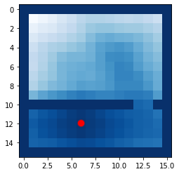
(c)

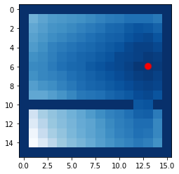
(d)

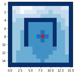
(e)

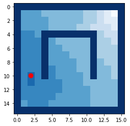
(f)

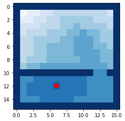
(g)

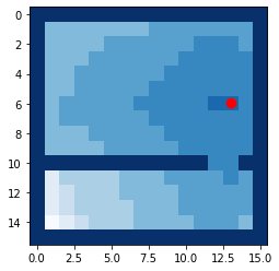
(h)

Figure 3: An illustration of goal-conditioned state space partitions for two simple Grid World navigation tasks. In each instance, the desired goal is represented by a red circle. In these environments, each state simply corresponds to a position on the grid and, in the top row, is colour-coded according to its goal-conditional value. In the lower row, states sharing similar values have been merged to form a partition. For any given state, the proposed target region advantage up-weights actions that move the agent directly towards a neighboring region with higher-value.

The results for Gym Robotics suite are shown in Table 3. For each algorithm, we report the average return and the standard deviation obtained from $5$ independent runs, each one using a different seed. As can be seen from the results, most of the competing algorithms reach a comparable performance with DAWOG. However, DAWOG generally achieves higher scores and the most stable performance in different tasks.

Analogous results for the AntMaze suite are shown in Table 3. Here, DAWOG outperforms all baselines as these are long-horizon and significantly more challenging environments. In diverse goal setting all algorithms under-perform, but DAWOG still achieves the highest average score. This setup requires better generalisation performance given that the test goals are sampled from every position within the maze. To gain an appreciation for the benefits introduced by the target region approach, in Figure 1 we visualise $100$ trajectories realised by three different policies for AntMaze tasks: dual-advantage weighting (DAWOG), equally-weighting and goal-conditioned advantage weighting. The trajectories generated by equally-weighting occasionally lead to regions in the maze that should have been avoided, which results in sub-optimal solutions. The policy from goal-conditioned advantage weighting is occasionally less prone to making the same mistakes, although it still suffers from the multi-modality problem. This can be appreciated, for instance, by observing the antmaze-medium case. In contrast, DAWOG is generally able to reach the goal with fewer detours, hence in a shorter amount of time.

5.5 Ablation studies

In this Section we take a closer look at how the two advantage-based weights featuring in Eq. 14 perform, both separately and jointly taken, when used in the loss of Eq. 13. We compare learning curves, region occupancy times (i.e. time spent in each region of the state space whilst reaching the goal), and potential overestimation biases.

5.5.1 Learning curves

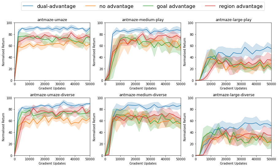
Figure 4: Training curves for different tasks using different algorithms, each one implementing a different weighting scheme: dual-advantage, no advantage, only goal-conditioned advantage, and only the target region advantage.

In the AntMaze environments, we train DAWOG using no advantage ($\beta=\tilde{\beta}=0$), only the goal-conditioned advantage ($\beta=10,\tilde{\beta}=0$), only the target region advantage ($\beta=0,\tilde{\beta}=10$), and the proposed dual-advantage ($\beta=\tilde{\beta}=10$). Figure 4 presents the corresponding learning curves over $50,000$ gradient updates. Both the goal-advantage and region-based advantage perform better than using no advantage, and their performance is generally comparable, with the latter often achieving higher normalised returns. Combining the two advantages leads to significantly higher returns than any advantage weight individually taken.

5.5.2 Region occupancy times

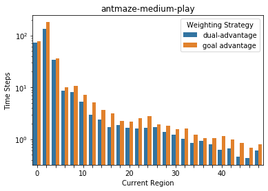
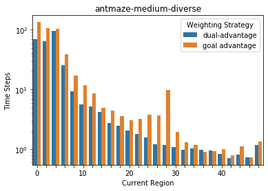
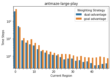
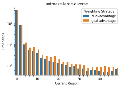
Figure 5: Average time spent in a region of the state space before moving on to the higher-ranking region ($K=50$) using a goal-conditioned value function for state partitioning. The $y$-axis indicates the average number of time steps (in log scale) spent in a region. The dual-advantage weighting scheme allows the agent to reach each subsequent target region more rapidly compared to the goal-conditioned advantage alone, which results in overall shorter time spent to reach the final goal.

In this study, we set out to confirm that the dual-advantage weighting scheme results in a policy favouring actions leading to the next higher ranking target region rapidly, i.e. by reducing the occupancy time in each region. Using the AntMaze environments, Figure 5 shows the average time spent in a region of the state space partitioned with $K=50$ regions. As shown here, the dual-advantage weighting allows the agent to reach the target (next) region in fewer time steps compared to the goal-conditioned advantage alone. As the ant interacts with the environment within an episode, the available time to complete the task decreases. Hence, as the ant progressively moves to higher ranking regions closer to the goal, the occupancy times decrease.

5.5.3 Over-estimation bias

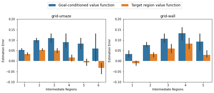
Figure 6: Estimation error of goal-conditioned and target region value functions in Grid World tasks.

We assess the extent of potential overestimation errors affecting the two advantage weighting factors used in our method (see Eq. 14). This is done by studying the error that occurred in the estimation of the corresponding V-functions (see Eq. 15 and Eq. 18). Given a state $s$ and goal $g$, we compute the goal-conditioned V-value estimation error as $V_{\psi_{1}}(s,g)-V^{\pi}(s,g)$, where $V_{\psi_{1}}(s,g)$ is the parameterised function learnt by our algorithm and $V^{\pi}(s,g)$ is an unbiased Monte-Carlo estimate of the goal-conditioned V-function’s true value sutton2018reinforcement . Since $V^{\pi}(s,g)$ represents the expected discounted return obtained by the underlying behaviour policy that generates the relabelled data, we use a policy pre-trained with the GCSL algorithm to generate $1,000$ trajectories to calculate the Monte-Carlo estimate (i.e. the average discounted return). Analogously, the target region V-value estimation error is $\tilde{V}_{\psi_{2}}(s,g,G(s,g))-\tilde{V}^{\pi}(s,g,G(s,g))$. We use the learnt target region V-value function to calculate $\tilde{V}_{\psi_{2}}(s,g,G(s,g))$, and Monte-Carlo estimation to approximate $\tilde{V}^{\pi}(s,g,G(s,g))$.

We present experimental results for the Grid World environment, which contains two layouts, i.e., grid-umaze and grid-wall. For each layout, we randomly sample $s$ and $g$ uniformly within the entire maze and ensure that the number of regions separating them is uniformly distributed in $\{1,\ldots,K\}$. Then, for each $k$ in that range: 1) $1,000$ goal positions are sampled randomly within the whole layout; 2) for each goal position, the state space is partitioned according to $V_{\psi}(\cdot,g)$; and 3) a state is sampled randomly within the corresponding region. Since there may exist regions without any states, the observed total number of regions is smaller than $K=10$. The resulting estimation errors are shown in Fig. 6. As can be seen here, both the mean and standard deviation of the $\tilde{V}$-value errors are consistently smaller than those corresponding to the $V$-value errors. This indicates the target region value function is more robust against over-estimation bias, which may help improve the generalisation performance in out-of-distribution settings.

5.6 Sensitivity to hyperparameters

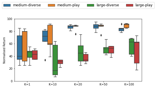
Figure 7: DAWOG’s performance, evaluated on the AntMaze dataset, as a function of $K$, the number of state space partitions required to define the target regions. The box plot of the normalised return in AntMaze task is achieved by DAWOG in four settings when the target region size decreases ($K$ increases). We used five runs with different seeds. Best performance (highest average returns and lowest variability) was consistently achieved across all settings with around $K=50$ equally sized target regions.

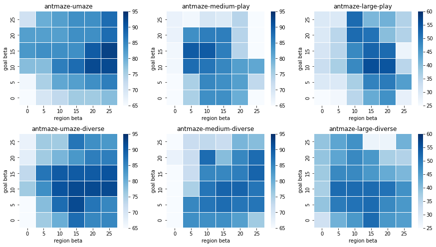
Figure 8: DAWOG’s performance, evaluated on six datasets, as a function of its two hyperparameters, $\beta$ and $\tilde{\beta}$, controlling the goal-conditioned and target-based exponential weights featuring in Equation 14. The performance metric is the average return across 5 runs. To produce the results presented in Table 3, we used a (potentially sub-optimal) fixed parameter combination: $\beta=10$ and $\tilde{\beta}=10$.

Lastly, we examine the impact of the number of partitions ($K$) and the coefficients $\beta$ and $\tilde{\beta}$, which control the relative contribution of the two advantage functions on DAWOG’s overall performance. In the AntMaze task, we report the distribution of normalized returns as $K$ increases. Figure 7 reveals that an optimal parameter yielding high average returns with low variance often depends on the specific task and is likely influenced by the environment’s complexity.

Figure 8 illustrates DAWOG’s performance as a function of $\beta$ and $\tilde{\beta}$. The plot demonstrates some minimal sensitivity to various parameter combinations but also exhibits a good degree of symmetry. In all our experiments, including those in Tables 3 and 3, we opted for a shared value, $\beta=\tilde{\beta}=10$, rather than optimizing each parameter combination for each task. This choice suggests that strong performance can be achieved even without extensive hyperparameter optimization.

6 Discussion and conclusions

We propose a dual-advantage weighting scheme for supervised learning to address multi-modality and distribution shift challenges in goal-conditioned offline reinforcement learning (GCRL). The corresponding algorithm, DAWOG (Dual-Advantage Weighting for Offline Goal-conditioned learning), prioritizes actions that lead to higher-reward regions, introducing an additional source of inductive bias and enhancing the ability to generalize learned skills to novel goals. Theoretical support is provided by demonstrating that the derived policy is never inferior to the underlying behavior policy. Empirical evidence shows that DAWOG learns highly competitive policies and surpasses several existing offline algorithms on demanding goal-conditioned tasks. Furthermore, DAWOG is easy to implement and train, making it a valuable contribution to advancing our understanding of offline GCRL and its relationship with goal-conditioned supervised learning (GCSL).

Future developments can explore various aspects of the proposed approach. Firstly, our current method partitions states into equally-sized bins for the value function. Implementing an adaptive partitioning technique that does not assume equal bin sizes could provide finer control over state partition shapes (e.g., merging smaller regions into larger ones), potentially leading to further performance improvements.

Secondly, considering DAWOG’s effectiveness in alleviating the multi-modality problem in offline GCRL, it may also benefit other GCRL approaches beyond advantage-weighted GCSL. Specifically, our method could extend to actor-critic-based offline GCRL, such as TD3-BC fujimoto2021minimalist , which introduces a behavior cloning-based regularizer into the TD3 algorithm fujimoto2018addressing to keep the policy closer to actions experienced in historical data. The dual-advantage weighting scheme could offer an alternative direction for developing a TD3-based algorithm for offline GCRL.

Lastly, given our method’s ability to accurately weight actions, it might also facilitate exploration in online GCRL, potentially in combination with self-imitation learning oh2018self ; ferret2021self ; li2022phasic . For example, a recent study demonstrated that advantage-weighted supervised learning is a competitive method for learning from good experiences in GCRL settings li2022phasic . These promising directions warrant further exploration.

References

- \bibcommenthead
- (1) Liu, M., Zhu, M., Zhang, W.: Goal-conditioned Reinforcement Learning: Problems and Solutions. In: International Joint Conference on Artificial Intelligence (2022)
- (2) Plappert, M., Andrychowicz, M., Ray, A., McGrew, B., Baker, B., Powell, G., Schneider, J., Tobin, J., Chociej, M., Welinder, P., Kumar, V., Zaremba, W.: Multi-goal Reinforcement Learning: Challenging Robotics Environments and Request for Research (2018)
- (3) Andrychowicz, M., Wolski, F., Ray, A., Schneider, J., Fong, R., Welinder, P., McGrew, B., Tobin, J., Abbeel, P., Zaremba, W.: Hindsight Experience Replay. In: Advances in Neural Information Processing Systems (2017)
- (4) Eysenbach, B., Zhang, T., Levine, S., Salakhutdinov, R.: Contrastive Learning as Goal-conditioned Reinforcement Learning. In: Advances in Neural Information Processing Systems (2022)
- (5) Mezghani, L., Sukhbaatar, S., Bojanowski, P., Lazaric, A., Alahari, K.: Learning Goal-conditioned Policies Offline with Self-supervised Reward Shaping. In: Conference on Robot Learning (2022)
- (6) Chebotar, Y., Hausman, K., Lu, Y., Xiao, T., Kalashnikov, D., Varley, J., Irpan, A., Eysenbach, B., Julian, R., Finn, C., Levine, S.: Actionable Models: Unsupervised Offline Reinforcement Learning of Robotic Skills. In: International Conference on Machine Learning (2021)
- (7) Ghosh, D., Gupta, A., Reddy, A., Fu, J., Devin, C.M., Eysenbach, B., Levine, S.: Learning to Reach Goals via Iterated Supervised Learning. In: International Conference on Learning Representations (2021)
- (8) Emmons, S., Eysenbach, B., Kostrikov, I., Levine, S.: RvS: What is Essential for Offline RL via Supervised Learning? In: International Conference on Learning Representations (2022)
- (9) Yang, R., Lu, Y., Li, W., Sun, H., Fang, M., Du, Y., Li, X., Han, L., Zhang, C.: Rethinking Goal-conditioned Supervised Learning and its Connection to Offline RL. In: International Conference on Learning Representations (2022)
- (10) Fu, J., Kumar, A., Nachum, O., Tucker, G., Levine, S.: D4RL: Datasets for Deep Data-Driven Reinforcement Learning (2020)
- (11) Fang, M., Zhou, T., Du, Y., Han, L., Zhang, Z.: Curriculum-guided Hindsight Experience Replay. In: Advances in Neural Information Processing Systems (2019)
- (12) Yang, R., Fang, M., Han, L., Du, Y., Luo, F., Li, X.: MHER: Model-based Hindsight Experience Replay. In: Deep RL Workshop NeurIPS 2021 (2021)
- (13) Jurgenson, T., Avner, O., Groshev, E., Tamar, A.: Sub-goal Trees: a Framework for Goal-based Reinforcement Learning. In: International Conference on Machine Learning (2020)
- (14) Nasiriany, S., Pong, V., Lin, S., Levine, S.: Planning with Goal-conditioned Policies. In: Advances in Neural Information Processing Systems (2019)
- (15) Nair, A.V., Pong, V., Dalal, M., Bahl, S., Lin, S., Levine, S.: Visual Reinforcement Learning with Imagined Goals. In: Advances in Neural Information Processing Systems (2018)
- (16) Durugkar, I., Tec, M., Niekum, S., Stone, P.: Adversarial Intrinsic Motivation for Reinforcement Learning. In: Advances in Neural Information Processing Systems (2021)
- (17) Charlesworth, H., Montana, G.: PlanGAN: Model-based Planning with Sparse Rewards and Multiple Goals. In: Advances in Neural Information Processing Systems (2020)
- (18) Kumar, A., Zhou, A., Tucker, G., Levine, S.: Conservative Q-learning for Offline Reinforcement Learning. In: Advances in Neural Information Processing Systems (2020)
- (19) Fujimoto, S., Gu, S.: A Minimalist Approach to Offline Reinforcement Learning. In: Advances in Neural Information Processing Systems (2021)
- (20) Ding, Y., Florensa, C., Abbeel, P., Phielipp, M.: Goal-conditioned Imitation Learning. In: Advances in Neural Information Processing Systems (2019)
- (21) Ho, J., Ermon, S.: Generative Adversarial Imitation Learning. In: Advances in Neural Information Processing Systems (2016)
- (22) Bain, M., Sammut, C.: A Framework for Behavioural Cloning. In: Machine Intelligence 15, pp. 103–129 (1995)
- (23) Peng, X.B., Kumar, A., Zhang, G., Levine, S.: Advantage-weighted Regression: Simple and Scalable Off-policy Reinforcement Learning (2019)
- (24) Wang, Q., Xiong, J., Han, L., sun, p., Liu, H., Zhang, T.: Exponentially Weighted Imitation Learning for Batched Historical Data. In: Advances in Neural Information Processing Systems (2018)
- (25) Li, J., Tang, C., Tomizuka, M., Zhan, W.: Hierarchical Planning through Goal-conditioned Offline Reinforcement Learning (2022)
- (26) Chane-Sane, E., Schmid, C., Laptev, I.: Goal-conditioned Reinforcement Learning with Imagined Subgoals. In: International Conference on Machine Learning (2021)
- (27) Kim, J., Seo, Y., Shin, J.: Landmark-guided Subgoal Generation in Hierarchical Reinforcement Learning. In: Advances in Neural Information Processing Systems (2021)
- (28) Zhang, L., Yang, G., Stadie, B.C.: World Model as a Graph: Learning Latent Landmarks for Planning. In: International Conference on Machine Learning (2021)
- (29) Ma, X., Zhao, S.-Y., Yin, Z.-H., Li, W.-J.: Clustered Reinforcement Learning (2020)
- (30) Wei, H., Corder, K., Decker, K.: Q-learning Acceleration via State-space Partitioning. In: International Conference on Machine Learning and Applications (2018)
- (31) Karimpanal, T.G., Wilhelm, E.: Identification and Off-policy Learning of Multiple Objectives using Adaptive Clustering. Neurocomputing 263, 39–47 (2017)
- (32) Mannor, S., Menache, I., Hoze, A., Klein, U.: Dynamic Abstraction in Reinforcement Learning via Clustering. In: International Conference on Machine Learning (2004)
- (33) Ghosh, D., Singh, A., Rajeswaran, A., Kumar, V., Levine, S.: Divide-and-conquer Reinforcement Learning. In: International Conference on Learning Representations (2018)
- (34) Kaelbling, L.P.: Learning to Achieve Goals. In: International Joint Conference on Artificial Intelligence (1993)
- (35) Schaul, T., Horgan, D., Gregor, K., Silver, D.: Universal Value Function Approximators. In: International Conference on Machine Learning (2015)
- (36) Sutton, R.S., Barto, A.G.: Reinforcement Learning: An Introduction. MIT press, Cambridge, MA, USA (2018)
- (37) Mnih, V., Kavukcuoglu, K., Silver, D., Rusu, A.A., Veness, J., Bellemare, M.G., Graves, A., Riedmiller, M., Fidjeland, A.K., Ostrovski, G., et al.: Human-level Control through Deep Reinforcement Learning. nature 518(7540), 529–533 (2015)
- (38) Lillicrap, T.P., Hunt, J.J., Pritzel, A., Heess, N.M.O., Erez, T., Tassa, Y., Silver, D., Wierstra, D.: Continuous Control with Deep Reinforcement Learning. In: International Conference on Learning Representations (2016)
- (39) Raffin, A., Hill, A., Gleave, A., Kanervisto, A., Ernestus, M., Dormann, N.: Stable-baselines 3: Reliable Reinforcement Learning Implementations. Journal of Machine Learning Research 22(268), 1–8 (2021)
- (40) Kingma, D.P., Ba, J.: Adam: A Method for Stochastic Optimization (2014)
- (41) Fujimoto, S., Meger, D., Precup, D.: Off-policy Deep Reinforcement Learning without Exploration. In: International Conference on Machine Learning (2019)
- (42) Fujimoto, S., Hoof, H., Meger, D.: Addressing Function Approximation Error in Actor-critic Methods. In: International Conference on Machine Learning (2018)
- (43) Mandlekar, A., Ramos, F., Boots, B., Savarese, S., Fei-Fei, L., Garg, A., Fox, D.: IRIS: Implicit Reinforcement without Interaction at Scale for Learning Control from Offline Robot Manipulation Data. In: International Conference on Robotics and Automation (2020)
- (44) Oh, J., Guo, Y., Singh, S., Lee, H.: Self-imitation Learning. In: International Conference on Machine Learning (2018)
- (45) Ferret, J., Pietquin, O., Geist, M.: Self-imitation Advantage Learning. In: International Conference on Autonomous Agents and Multiagent Systems (2021)
- (46) Li, Y., Gao, T., Yang, J., Xu, H., Wu, Y.: Phasic Self-imitative Reduction for Sparse-reward Goal-conditioned Reinforcement Learning. In: International Conference on Machine Learning (2022)