Well-posedness of Partially and Oblique Projected Dynamical Systems

I HIGS

The general form of the hybrid integrator, extending the description of HIGS in [DeeSha_AUT21a], is mathematically formulated as the scalar-state switched nonlinear system

$$\dot{x}_{h} =f(x_{h},e),\hphantom{k_{h}z}\textup{ if }\left(e,u,\dot{e}\right)\in\mathcal{F}_{1},$$ (1a)

$${x}_{h} =k_{h}e,\hphantom{f(x_{h},z)}\textup{ if }\left(e,u,\dot{e}\right)\in\mathcal{F}_{2},$$ (1b)

$$u =x_{h},$$ (1c)

with state $x_{h}(t)\in\mathbb{R}$, input $e(t)\in\mathbb{R}$, output $u(t)\in\mathbb{R}$ at time $t\in\mathbb{R}_{\geq 0}$, and where $f:\mathbb{R}\times\mathbb{R}\to\mathbb{R}$ is a nonlinear function. Here, $\dot{e}$ denotes the time-derivative. The flow sets $\mathcal{F}_{1}$ and $\mathcal{F}_{2}$ dictating the active mode in (1) are given by

$$\mathcal{F}_{1} :=\left\{(e,u,\dot{e})\in\mathbb{R}^{3}\mid eu\geq\frac{u^{2}}{k_{h}}\wedge(e,u,\dot{e})\not\in\mathcal{F}_{2}\right\},$$ (2a)

$$\mathcal{F}_{2} :=\left\{(e,u,\dot{e})\in\mathbb{R}^{3}\mid u=k_{h}e\wedge f(x_{h},e)e>k_{h}\dot{e}e\right\}$$ (2b)

of which the union forms the $[0,k_{h}]$-sector defined as

$$\mathcal{F}:=\mathcal{F}_{1}\cup\mathcal{F}_{2}=\left\{(e,u,\dot{e})\in\mathbb{R}^{3}\mid eu\geq\frac{u^{2}}{k_{h}},\dot{e}\in\mathbb{R}\right\}.$$ (3)

The sets $\mathcal{F}_{1}$ and $\mathcal{F}_{2}$ in (2) define regions where $\mathcal{H}$ operates in either a dynamic mode or a static mode. The dynamic mode is referred to as ‘integrator-mode’, since, essentially, the state value $x_{h}$ is obtained from integration. The static mode is soemtimes referred to as ‘gain-mode’. Note that the definition of the set $\mathcal{F}$ in (3) shows the input-output pair $(z,u)$ of the hybrid integrator in (1) to have an equivalent sign at all times, which may benefit transient properties of a closed-loop system. For a further motivation of the sets in (2), along with a visualization, the reader is referred to [DeeSha_AUT21a, Section 3].

Note that (1b) is in the form of a (differential) algebraic equation. We could replace this by an ODE, which then turns (1) into

$$\dot{x}_{h} =f(x_{h},e),\hphantom{k_{h}z}\textup{ if }\left(e,u,\dot{e}\right)\in\mathcal{F}_{1},$$ (4a)

$$\dot{x}_{h} =k_{h}\dot{e},\hphantom{f(x_{h},z)}\textup{ if }\left(e,u,\dot{e}\right)\in\mathcal{F}_{2},$$ (4b)

$$u =x_{h},$$ (4c)

directly revealing also the dependence of the right-hand sides on $\dot{e}$ (in the gain mode).

Concerning the vector field in (1a), the following assumptions are made.

Assumption 1.

The function $f$ in (1) satisfies $f(0,0)=0$, and $f(0,e)e\geq 0$ for all $e\in\mathbb{R}$.

II Open-loop formulation of projection-based controllers: HIGS as sweeping process

II-A Sweeping process

Let us first consider the classical HIGS in which $f(x_{h},e)=e$. We can write this as the sweeping process [REF], where we use that the normal cone for a given set $K\subseteq\ree^{n}$ at $x\in K$ is defined as

$$N_{K}(x)=\{s\in\ree^{n}\mid\langle s\mid k-x\rangle\leq 0\text{ for all }k\in K\}.$$ (5)

In case $x\not\in K$ then $N_{K}(x)$ is defined as the empty set.

We assume $e$ is given as a function of time.

$$\dot{x}_{h} \in \underbrace{f(x_{h},e(t))}_{\bar{f}(x_{h},t)}-N_{\bar{S}(t)}(x_{h})$$ (6a)

$$x_{h}(t) \in \bar{S}(t)$$ (6b)

with

$$\bar{S}(t)=\{x_{h}\in\ree\mid(e(t),x_{h})\in S\}$$ (7)

and $S$ is the sector corresponding to $\mathcal{F}$ defined by

$$S=\left\{(e,u)\in\mathbb{R}^{2}\mid eu\geq\frac{u^{2}}{k_{h}}\right\}.$$ (8)

II-B Equivalence of HIGS and SP

Indeed, note that

$$\bar{S}(t)=\begin{cases}[0,k_{h}e(t)],&\text{when }e(t)\geq 0,\\ [k_{h}e(t),0],&\text{when }e(t)\leq 0,\end{cases}$$ (9)

which are convex sets (in fact, closed intervals of the real line) for each $t$.

Note that

$$d_{Haus}(\bar{S}(t_{1}),\bar{S}(t_{2}))\leq k_{h}|e(t_{1})-e(t_{2})|$$

for all $t_{1},t_{2}$ [check!]. So, by imposing an AC condition on $e$ we get the required regularity on the set $\bar{S}$.

Solutions are guaranteed now to (6) by [Edmond, Thibault].

Observe that for $x\in[a,b]$ and when $a<b$

$$N_{[a,b]}(x)=\begin{cases}\{0\},&\text{ when }x\in(a,b,)\\ \ree_{\leq 0},&\text{ when }x=a,\\ \ree_{\geq 0},&\text{ when }x=b.\end{cases}$$ (10)

Moreover when $a=b$, we get $N_{[a,a]}(x)=\ree$ for $x=a$.

MAURICE: Maybe we should prove existence to the first HIGS formulation and use uniqueness of solutions of the NC formulation/SP: suppose $f$ is locally Lipschitz , then take two solutions to SP $x,\tilde{x}$, then

$$d/dt|x(t)-\tilde{x}(t)|^{2}\leq 2L|x(t)-\tilde{x}(t)|^{2}$$

as normal cone is monotone. So uniqueness of solutions. a solution to HIGS is a solutions to SP/NC so if we can prove existence of solutions to HIGS – e.g. with arguments later via Krasovskii??? maybe we can apply them in open -loop, we show that HIGS is a sweeping process

Maurice we do not get right away that the formuled sweeping process model with the normal cone is equal to the MODEL of HIGS above – only the “slow/lazy” solution matches the HIGS formulation - -some work needed to clarify this !!! Note that also taking the minimal norm/projection on Normal cone of the right-hand side in (6a) is not helping! There is no way how a $\dot{e}$ gets in this by just looking at the right-hand sides and doing calculus on that [see some calculus below], it is really a consequence of the solution satisfying (6b) as well and hence $\dot{x}_{h}$ somehow has to lie in the tangent cone! This result on PDS - normal cone equivalence is for constant constraint sets, I guess, see [BROGLIATO2006, heemelsorl]

Take the case $e(t)>0$ and thus $\bar{S}(t)=[0,k_{h}e(t)]$ and take $x_{h}=k_{h}e(t)$ (so on the boundary), and $N_{\bar{S}(t)}(x_{h})=\ree_{\geq 0}$ in this case. Hence, (6a) reads $\dot{x}_{h}\in f-\ree_{\geq 0}$. By now taking the minimal norm solution of the r.h.s. for $f=e$ we do get $\dot{e}$ in. So, this is not a ”static” property of the r.h.s., but it is due to the fact that (6b) has to hold and thus some viability/tangent cone condition kicks in due to time-varying nature of $\bar{S}$ , i.e. $\dot{x}_{h}\leq k_{h}\dot{e}(t)$ has to hold, and this dynamic condition is going to be important [somehow this is a tangent cone condition to $S$, which appears in Section III]. I guess a minimal norm solution kicks in under this constraint! hence, the time-varying nature of $\bar{S}$ (and loosely speaking the ”derivative” of the set, related to $\dot{e}$) plays a role! I will start digging in the works that you mentioned of Thibault and your observer paper, etc.

BTW: I do believe the sweeping process formulation (6) and the HIGS-based formulations (1) or (4) have the same solutions!!!!!!!! only we need to find the proper setting to connect the two!!

II-C Well-posedness

As shown above, first some work needed to embed the HIGS equations (1) or (4) in an appropriate mathematical (sweeping process framework). If accomplished, then following questions arise:

• Can we rely on classical results for well-posedness? Locally AC inputs give local existence and uniqueness?

• global existence of solutions?

• consistency of a time-stepping scheme? how does the particular time-stepping scheme look if we translate it from classical literature?

• we could also directly make the step in the projection-based controller to state $x_{h}\in\ree^{n_{h}}$ and put the sector constraint on its input-output pair! see below

III Direct Closed-loop formulations of projection-based controllers: ePDS

Plant (+ smooth controller part) and projection-based controller (with state $x_{h}$

$$\dot{x}_{p} = f_{p}(x_{p},u,w)=f_{p}(x_{p},g_{h}(x_{h}),w);\ e=g_{p}(x_{p})$$

$$\dot{x}_{h} = f_{h}(x_{h},g_{p}(x_{p}));\ u=g_{h}(x_{h})$$

We write this as

$$\dot{x}=F(x,w)$$ (11)

Then

$$\dot{x}=\Pi_{S,E}(x,F(x,w))$$ (12)

with $n=n_{p}+n_{h}$

$$S=\left\{x\in\mathbb{R}^{n}\mid e=g_{p}(x_{p}),u=g_{h}(x_{x}),eu\geq\frac{u^{2}}{k_{h}}\right\}.$$ (13)

$$E=[0\ I]^{\top}$$ (14)

$$\Pi_{S,E}(x,v)=\operatorname{argmin}_{w\in T_{S}(x),w-v\in\im E}\|w-v\|$$ (15)

This is a mathematical framework that fits and we can show that this leads to the description (4) [with $f=e$] in closed loop with the plant dynamics. See [DeeSha_AUT21a] [using a PWL modelling formalism]. Also here we obtain global existence of solutions w.r.t. bounded piecewise Bohl inputs (including forward completeness), using lexicographic orderings of derivatives in Taylor expansions.

Note that with respect to classical PDS there are essential differences:

• projection is not complete in the sense that only some directions (not all) can be used to keep the state in the constraint set $S$

• using a non-convex constraint set $S$ (note as opposed to setup in Section II, this is now a constant set, not dependent on time).

In case all the states can be altered/projected, $S$ is convex and no inputs are present, we recover as a special case of the above framework the classical PDS.

III-A HIGS special case

Maybe first for HIGS or at least the FOPE – with $u=x_{h}$ and $n_{h}=1$

• is the ePDS formulation well-posed in the sense that projection operator is well defined? see some conditions below that are needed. Assumption 2.

• existence / uniqueness of solutions, see [DeeSha_AUT21a] for piecewise Bohl inputs.

• MAURICE can this be written as an interconnection of sweeping process and smooth nonlinear $x_{p}$ dynamics?, i.e. is the ”direct closed-loop formulation” here ”similar”/same to using the HIGS/FOPE interconnected with smooth system $\rightarrow$ can we use 2nd order sweeping processes here???? This might work – we typically use a relative degree assumptions, i.e. the external disturbance $w$ is not directly present in $e=g_{p}(x_{p})$. so, at least relative degree 1. We can even assume relative degree 2, if this helps!

Regarding the latter item: I would expect something like

$$\dot{x}_{p} = =f_{p}(x_{p},g_{h}(x_{h}),w);$$ (16a)

$$\dot{x}_{h} = f_{h}(x_{h},g_{p}(x_{p}))-N_{\tilde{S}(g_{p}(x_{p}))}(x_{h}),$$ (16b)

where

$$\tilde{S}(g_{p}(x_{p}))=\{x_{h}\in\ree\mid(g_{p}(x_{p}),x_{h})\in S\}$$ (17)

with $S$ the sector-like set defined before. Does this fit directly the state-dependent 2nd order sweeping process formulation? Does this connect to your observer design paper with Bernard and Christophe?

Can we use this prove existence (and maybe uniqueness) of solutions for Lebesgue measurable or AC external disturbance inputs?

And what about time-stepping schemes with consistence?

III-B General case

What about the general case ($n_{h}>1$) ? same questions as above.

III-C State-dependent norms?

$$\Pi_{S,E}(x,v)=\operatorname{argmin}_{w\in T_{S}(x),w-v\in\im E}\|w-v\|_{P(x)}$$ (18)

with $P(x)\succ 0$ or maybe even $E(x)$? See Hauswirth paper where they look at what they call oblique PDS – full projection but metric $\|\cdot\|_{P(x)}$ in projection operator state-dependent. Connection to that work?

III-D Well-posedness

can we prove existence/uniqueness of solutions? what are natural classes of inputs?

I have been working on a viability/aubin/cellina type of approach, good to connect to that!

Viability condition for regularized dynamics $\dot{x}=\text{Kras}(\Pi)$ (we apply regularization to get osc properties) is $\text{Kras}(\Pi)\cap T_{s}\neq\emptyset$. Moreover, every solution to the regularized dynamics has to satisfy $\dot{x}=\text{Kras}(\Pi)\cap T_{s}$. To show that this is a solution to the original (non-regularized) dynamics, it would be sufficient to show

$$\text{Kras}(\Pi)\cap T_{s}=\Pi$$

Does this hold?

In general it is not true that

$$\text{Kras}(\Pi)=F-N_{S}$$

We found examples for $e=x_{h}=u=0$ and $\dot{e}>0$ but fortunately these are isolated points in time. In fact, this is caused by $x\mapsto T_{S}(x)$ not being lower semicontinuous!!! maybe nice to add an example illustrating this!

This would lead to the question if $\text{Kras}(\Pi)\cap T_{s}=\Pi$ is connected to take the slowest solutions in the normal cone DI? same line of reasoning, would be great to connect those – where Aubin meets Moreau?

IV Toulouse 20230203

IV-A Time-invariant case

Let $K$ be a convex polyhedral set given and a linear subspace ${\cal E}=\im E$ where $E\in\ree^{n\times n_{E}}$ is a matrix with full column rank. Moreover, we assume

Assumption 2.

The set $K\subseteq\ree^{n}$ and ${\cal E}$ satisfy

• $K=\{x\in\ree^{n}\mid Hx\geq b\}$ for some matrix $H\in\ree{n_{H}\times n}$ MH: rank condition on active constraints? and vector $b\in\ree^{n}$

• ${\cal E}+T_{K}(x)=\ree^{n}$ for all $x\in K$ (in case $K$ is pointed convex cone, then ${\cal E}+K=\ree^{n}$, equivalent - nice to have a more general condition on $K$)

$$\Pi_{K,{\cal E}}(x,v)=\operatorname{argmin}_{w\in T_{K}(x),w-v\in{\cal E}}\|w-v\|$$ (19)

Under Assumption 2 $\{\w\in T_{K}(x)\mid w-v\in{\cal E}\}$ is nonempty, closed and convex. According to the closest point theorem [Luenberger] there is a unique minimizer, so the projection operator above is well-defined.

$$\dot{x}=\Pi_{K,{{\cal E}}}(x,f(x))=:F(x)$$ (20)

Assumption 3.

$f$ is a continuous mapping in $x$ .

Active constraint index set $J(x):=\{i\mid H_{i}x=b_{i}\}$. Then $T_{K}(x)=\{v\mid H_{J}v\geq 0\}$. For convenience we introduce $T_{J}:=\{v\mid H_{J}v\geq 0\}$ for $J\subseteq\{1,\ldots,n_{N}\}.$

MH: [we can probably extend all of this $K$ given by mapping $H(x)\geq 0$.] using $gradH_{i}$

Consider the Krasovskii regularisation of (37) given by

$$\dot{x}\in\cap_{\delta>0}\overline{\textup{con}}F(B(x,\delta))=:K_{F}(x)$$ (21)

Above, $\overline{\textup{con}}(M)$ denotes the closed convex hull of the set $M$, in other words, the smallest closed convex set containing $M$.

Proposition 4.

If $f$ is continuous and Assumption 2 holds, then the Krasovskii regularization of $F$ at $x\in K$ is equal to

$$K_{F}(x)=\textup{con}\{P_{T_{J},{\cal E}}(f(x))\mid J\subset J(x)\}$$ (22)

MH: this result reveals the lower semicontinuity of $x\mapsto T_{K}(x)$ through the $J\subset J(x)$ – this property will be crucial in generalizing the result to general convex or even prox regular sets. However, this requires to find some useful extension of this proposition characterising the Krasovskii regularisation

$$K_{F}(x)\subseteq(?=?)\overline{\textup{con}}\bigcup\{P_{T,{\cal E}}(f(x))\mid T_{K}(x)\subset T,\ T\textup{closed, convex cone}\}$$ (23)

would this hold, at least with $\subseteq$? due to lsc of $T_{K}(x)$ all nearby $T_{K}(y)$ with $y\in B(x,\delta)$ satisfy $T_{K}(x)\subseteq T_{K}(y)+eps$ (”loosely speaking”). In fact, this can be used to generalize all the stuff below!

Theorem 5.

Assume that $f$ is continuous and Assumption 2 holds. Then for all $x\in K$ it holds that

$$K_{F}(x)\cap T_{K}(x)=\{F(x)\}=\{\Pi_{K,{{\cal E}}}(x,f(x))\}$$ (24)

Proof.

It is obvious that the inclusion $\supseteq$ holds as $\Pi_{K,{{\cal E}}}(x,f(x))$ clearly belongs to both $T_{K}(x)$ and $K_{F}(x)$ (cf. (50)). So, let us consider the reversed inclusion $\subseteq$. Thereto, let $v\in K_{F}(x)\cap T_{K}(x)$. Based on Proposition 4, $v\in K_{F}(x)$ can be written as

$$v=\sum_{J\subseteq J(x)}\lambda_{J}P_{T_{J},{\cal E}}(f(x))$$

with $\lambda_{J}\geq 0$, for $J\subset J(x)$, and $\sum_{J\subset J(x)}\lambda_{J}=1$. Let us consider

$$|v-f(x)|=|\sum_{J\subset J(x)}\lambda_{J}P_{T_{J},{\cal E}}(f(x))-f(x)|=\\ |\sum_{J\subseteq J(x)}\lambda_{J}P_{T_{J},{\cal E}}(f(x))-\sum_{J\subset J(x)}\lambda_{J}f(x)|\leq\\ \sum_{J\subseteq J(x)}\lambda_{J}|P_{T_{J},{\cal E}}(f(x))-f(x)|\leq\\ \sum_{J\subseteq J(x)}\lambda_{J}|P_{\underbrace{T_{J(x)}}_{T_{K}(x)},{\cal E}}(f(x))-f(x)|=\\ |P_{T_{J}(x),{\cal E}}(f(x))-f(x)|=|\Pi_{K,{{\cal E}}}(x,f(x))-f(x)|$$ (25)

where we used in the second inequality that $|P_{T_{J},{\cal E}}(f(x))-f(x)|\leq|P_{T_{J(x)},{\cal E}}(f(x))-f(x)|$ as $T_{J(x)}\subseteq T_{J}$. Moreover, by definition of $P_{T_{J},{\cal E}}$ it holds that $P_{T_{J},{\cal E}}(f(x))-f(x)\in{\cal E}$ for each $J\subset J(x)$ and thus also

$$\sum_{J\subseteq J(x)}\lambda_{J}(P_{T_{J},{\cal E}}(f(x))-f(x))=\underbrace{\sum_{J\subseteq J(x)}\lambda_{J}P_{T_{J},{\cal E}}(f(x))}_{=v}-f(x)\in{\cal E}$$

due to ${\cal E}$ being a linear subspace. Since $v\in T_{K}(x)$ and $v-f(x)\in{\cal E}$, and $|P_{T_{J(x)},{\cal E}}(f(x))-f(x)|$ is the shortest distance along ${\cal E}$ between $T_{J}(x)=T_{K}(x)$ and $f(x)$, i.e.,

$$\Pi_{K,{\cal E}}(x,f(x))=\operatorname{argmin}_{w\in T_{K}(x),w-f(x)\in{\cal E}}\|w-f(x)\|$$

it must hold that

$$|v-f(x)|=|\Pi_{K,{{\cal E}}}(x,f(x))-f(x)|$$

and thus $v$ must be the unique closest point in $T_{K}(x)$ to $v$ along ${\cal E}$ and thus $v=\Pi_{K,{{\cal E}}}(x,f(x))$, thereby proving the result. ∎

Theorem 6.

Assume that $f$ is continuous and Assumption 2 holds. Then for every initial condition $x(t_{0})=x_{0}\in K$ there exists $T>0$ and an AC solution $x:[0,T]\rightarrow K$ to (37). MH: under boundedness/growth conditions this should also be extended to global existence of solutions.

Proof.

Lemma 5.16 in [Goebel, sanfelice, teel book] show that $K_{F}$ is outer semicontinous and in case $F$ locally bounded then $K_{F}$ locally bounded. Moreover, $K_{F}$ takes closed and convex setvalues and for all $x\in K$ there is an open neighborhood $U$ of $x$ such that for all $y\in U\cap K$ it holds that $K_{F}(y)\cap T_{K}(y)\neq\emptyset$ (as it contains $\Pi_{K,{\cal E}}(y,f(y))$). According to Lemma 5.26 (b) [goebel, sanfelice, teel] [maybe better to refer to original Aubin source to, on viability theory] the corresponding viability conditions are satisfied implying that the Krasovskii regularization (50) has a solution $x$. Hence, this solution $x$ satisfies $x(t)\in K$ for all $t\in[O,T]$, it holds that $\dot{x}(t)\in T_{K}(x(t))$, almost everywhere, see Lemma 5.26 (a) [goebel, sanfelice, teel]. Hence, it holds a.e. that

$$\dot{x}(t)\in K_{F}(x(t))\cap T_{K}(x(t))$$ (26)

Invoking Theorem 5 shows that $x$ is now a solution to (37) as the right-hand side of (26) is contained of a single element being equal to the right-hand side of (37) are equal. ∎

MH Interestingly, this is an alternative way to prove existence of solutions to (ordinary) PDS using Krasovskii regularisation and viability theory contrasting other proofs building on Skoroghod problem [nagurney and zhang], plus other proofs – henry? who proved existence of solutions to PDS and how – of course viability results also build on time-stepping proofs… so maybe deep down the same?

IV-B Time-varying case

$$\dot{x}=f(x,t)$$

$f$ continuous in $x,t$

$$\dot{x}=\Pi_{K,{{\cal E}}}(x,f(x,t))=:F(x,t)$$ (27)

can we take $\bar{K}=\{(x,t)\mid x\in K\}$ still polyhedral convex set and $\bar{\cal E}=\bar{E}\times\{0\}$ (not allowed to project in $t$ direction). Define $\bar{f}(x,t)=(f(x,t),1)$). Is, with $\xi=(x,t)$,

$$\dot{x}=\Pi_{K,{{\cal E}}}(x,f(x,t))=:F(x,t)$$ (28)

”same” as

$$\dot{\xi}=\Pi_{\bar{K},\bar{{\cal E}}}(\xi,\bar{f}(\xi))=:\bar{F}(\xi)$$ (29)

$\bar{f}$ is continuous in $\xi$. so for continuous inputs we are good and we can concatenate to go to piecewise continuous.

IV-C Further extensions

Possible extensions

• prox regular sets $K$

• what if ${\cal E}={\cal E}(x)$ can depend on $x$ but in a continuous way…

• what if we do not use Euclidean norm $|\cdot|$ but state-dependent norms $|\cdot|_{P(x)}$ a la Hauswirth, with $P(x)$ positive definite and continuous in $x$, see details and motivation in Hauswirth’s papers

• time-varying $K(t)$??? maybe the embedding approach with $\dot{t}=1$ solves this already ;-)

V Beyond convexity and prox regularity: What about sector sets

In control theory often sector sets are of interest, see lure… etc etc.

Assumption 7.

The set $S\subseteq\ree^{n}$ and $E\in\ree^{n\times n_{E}}$ satisfy

• $S=K\cup-K$ in which $K$ is a convex polyhedral cone given by $K=\operatorname{pos}G+\im H$ in which the matrix $[G\ H]$ is square and has rank $n$

• $K\cap-K=\im G$

• $E$ full column rank

• $\im E\cap S=\{0\}$ and thus $S+\im E=\ree^{n}$

How can the above ideas be used to prove existence of solutions to

$$\dot{x}=\Pi_{S,E}(x,f(x))$$ (30)

with

$$\Pi_{S,E}(x,v)=\operatorname{argmin}_{w\in T_{S}(x),w-v\in\im E}\|w-v\|$$ (31)

for $x\in S$ and $v\in\ree^{n}$.

VI Aneel 20230204

MH: I start with simpler setup here, to see if we can make that work and then let us see if we generalize

suppose after a possible coordinate transformation we get:

$$\dot{x} = g(x,u);\ e=x_{n}$$

$$\dot{u} = h(u,e)$$

$\xi=(x,u)$ and then above reads $\dot{\xi}=f(\xi)$.

$$S=\left\{\xi\in\mathbb{R}^{n+1}\mid eu\geq\frac{u^{2}}{k_{h}}\right\}.$$ (32)

Denote for convenience the 2d sector as $\bar{S}$, i.e.

$$\bar{S}=\left\{(e,u)\in\mathbb{R}^{2}\mid eu\geq\frac{u^{2}}{k_{h}}\right\}.$$ (33)

$$T_{S}(\xi)=\ree^{n-1}\times T_{\bar{S}}(e,u)$$ (34)

Assumption 8.

$h(0,0)=0$

$${\cal E}=\textup{Im}[0\ 1]^{\top}$$ (35)

$$\dot{\xi}=\Pi_{S,{{\cal E}}}(\xi,f(\xi))=:F(\xi)$$ (36)

In fact,

$$\dot{\xi}=\begin{cases}\Pi_{K,{{\cal E}}}(\xi,f(\xi)),&\text{ when }\xi\in K\setminus-K\\ \Pi_{-K,{{\cal E}}}(\xi,f(\xi)),&\text{ when }\xi\in-K\setminus K\\ f(\xi),&\text{ when }\xi\in-K\cap K\end{cases}$$ (37)

The latter follows from the fact that $f_{h}(0,0)=0$ and therefore $f(\xi)\in T_{S}(\xi)$. MH: when generalizing to general 2d sectors this will differ

Although $K_{f}\cap T_{S}\neq\Pi$ here, we can still exploit the results in the preceding section to establish existence of solutions here.

Theorem 9.

An AC solutions exists locally for each initial state $\xi_{0}\in S$, i.e. on $[0,T]$ for some small positive $T$.

Proof.

MH: sketch for now Apply Krasovskii regularisation to $\dot{\xi}=F(\xi)$ and observe that $K_{F}(\xi)\cap T_{S}(\xi)\neq\emptyset$ for all $\xi\in S$. Hence, the local viability assumption is satisfied and we can establish for any initial state the existence of an AC solution $\xi:[0,T]\rightarrow S$ to $\dot{x}\in K_{F}(\xi)$. Clearly, due to the necessity of the viability condition, we obtain that the solution satisfies a.e.

$$\dot{\xi}\in K_{F}(\xi)\cap T_{S}(\xi)$$

. Interestingly, for all times $t\in[0,T]$ for which $\xi(t)\not\in K\cap-K$, we can use the results in the proceeding section that lead for these $t$ to

$$K_{F}(\xi(t))\cap T_{S}(\xi(t))=\Pi_{S,{\cal E}}(\xi(t),f(\xi(t)))$$ (38)

. In fact, for each such $t$ there is due to closedness of $K\cap-K$ and $\xi$ being continuous, some $\epsilon_{t}>0$ such that this must hold on $[t,t+\epsilon_{t}]$ Hence, we only have to consider the times where $\xi(t)\in K\cap-K$, i.e. $(e(t),u(t))=(0,0)$. We will differentiate two subcases: (i) $\dot{e}(t)\neq 0$ and (ii) $\dot{e}(t)=0$.

maybe consider only times where $\xi$ differentiable

Subcase (i): without loss of generality, let us assume $\dot{e}(t)>0$. Note that $\dot{e}=g_{n}(x,u)$ which [some properties of $g_{n}$ so that from AC $x,u$ we can conclude continuous $\dot{e}$]. Hence, we have that there is an $\epsilon_{t}$ and an $\eta>0$ such that $\dot{e}(\theta)\geq\eta$ for $\theta\in[t,t+\varepsilon_{t}]$. Hence, we have that $e(t)=0$, but $e(\theta)\geq\eta(\theta-t)>0$ for $\theta\in[t,t+\epsilon_{t}]$. Hence, the point where $e$ is zero is an isolated point (measure zero set), and for $\theta\in(t,t+\epsilon_{t}]$ $\xi(t)\in K\setminus-K$, for which (38) holds (with $t=\theta$).

Subcase (ii) $\dot{e}(t)=0$. Hence, we have that $\dot{e}(t)=g_{n}(x(t),u(t))=0$ and $\dot{u}(t)=h(0,0)=0$. Note that $(\dot{e}(t),\dot{u}(t))\in T_{\bar{S}}(0,0)$. The Krasovskii regularization eq:kras, recalled here for convenience,

$$\dot{x}\in\cap_{\delta>0}\overline{\textup{con}}F(B(x,\delta))=:K_{F}(x)$$ (39)

$F(\xi)=(g_{1}(\xi),..g_{n-1}(\xi),\Pi_{[01]^{\top},\bar{S}}((e,u),(g_{n},h))$

Can we express this krasovskii regularization as we did before with polyhedral sets??? that would be helpful, I guess we can do it!!!

So $K_{F}(\xi)=(g_{1}(\xi),..g_{n-1}(\xi))\times\textup{con}\{P_{T_{J},{\cal E}}((g_{n},h))\mid J...)\}$ where $T_{J}$ are appropriate tangent cones of points nearby $(e,u)=0$ and $(g_{n},h)=0$. Hence, $K_{F}(\xi)=\{(g_{1}(\xi),..g_{n-1}(\xi),0,0)\}=\Pi_{S,{\cal E}}(\xi,f(\xi))$.

Hence, in this case we have that for almost all $t\in[0,T]$

$$\dot{\xi}(t)=\Pi_{S,{\cal E}}(\xi(t),f(\xi(t)))$$

there establishing that $\xi$ is indeed an AC solution to the original pPDS. ∎

MH: let us find a good name for partially projected dynamical systems – is partial projection a good term? as opposed to oblique projection - used by hauswirth, although oblique projections as they are classically defined are possibly closer to partial projection ;-)

Corollary 10.

under lipschitz like bounds, we can prove global existence, i.e. on $[0,\infty)$ solutions

Proof.

concatenate, using lipschitz like bounds to avoid finite escape times. ∎

Corollary 11.

case of continuous inputs

Proof.

embed $t$ in it $\dot{t}=1$ and then for continuous input ∎

Corollary 12.

piecewise continuous inputs, make global results

Proof.

use previous corollary and concatenate, indicating that at continuities of $w$ you still are in the set $S$! so you can continue with a local solution, and as long as finite escape times are avoided we should be fine ∎

VII Toulouse 20230208

VII-A Introduction

VII-B Preliminaries on oblique projected dynamical systems

maybe first normal PDS and then e/o PDS

VII-C Projection-based controllers

Consider the general nonlinear single-input single-output (SISO) plant given by

$$\dot{x} = g(x,u)$$ (40a)

$$e = r(x)$$ (40b)

with state $x\in\ree^{n}$, control input $u\in\ree$ and output $e\in\ree$.

We will control this by a projection-based controller for which the unprojected dynamics are given by

$$\dot{z} = h(z,e)$$ (41a)

$$u = z_{1}$$ (41b)

with state $z\in\ree^{m}$, controller output $u\in\ree$ and controller input $e\in\ree$. Note that the controller output equation $u=z_{1}$ can be realizes under very mild assumptions by a coordinate transformation in case $u=s(z)$ for a function $s:\ree^{m}\rightarrow\ree$. to be added mild condition or reference! We assume that all the maps $g$, $r$ and $h$ are assumed to be continuous. Moreover, $r$ is assumed to be continuously differentiable. check actual needs after proofs!

The projection will take place only on controller states $z$ and the dynamics, as we cannot change the plant states and dynamics as they adhere to physical laws, resulting in an oblique or partial projection operation with the goal to keep the input-output pair $(e,u)$ in a sectorset

$$S=\left\{(e,u)\in\mathbb{R}^{2}\mid(u-k_{1}e)(u-k_{2}e)\leq 0\right\},$$ (42)

where $k_{1},k_{1}\in\ree$ with $k_{1}<k_{2}$. We can write $S$ also as the union of two polyhedral cones

$$S=K\cup-K$$ (43)

with

$$K=\left\{(e,u)\in S\mid e\geq 0\right\}=\left\{(e,u)\in\ree^{2}\mid u\geq k_{1}e\text{ and }u\leq k_{2}e\right\}.$$

To write the closed-loop system description we introduce the state $\xi=(x,z)\in\ree^{n+m}$, the constraint set $S$ on the level of the states $\xi$ as

$${\cal S}=\left\{\xi=(x,z)\in\mathbb{R}^{n+m}\mid e=r(x),\ u=z_{1},\ (e,u)\in S\right\},$$ (44)

and the projection subspace as

$${\cal E}=\textup{Im}\begin{bmatrix}O_{n}\\ I_{m}\end{bmatrix}.$$ (45)

Note that we can also write ${\mathcal{S}}={\mathcal{K}}\cup-{\mathcal{K}}$ with ${\mathcal{K}}:=\left\{\xi=(x,z)\in\mathbb{R}^{n+m}\mid(e,u)\in K\right\}$.

The closed-loop dynamics can now be written as

$$\dot{\xi}=\Pi_{{\cal S},{\cal E}}(\xi,f(\xi)):=F(\xi)$$ (46)

with $f$ denoting the unprojected closed-loop dynamics given by

$$f(\xi)=(g(x,z_{1}),h(z,r(x))).$$ (47)

[for simplicity without external input $w$, but we can aim for embedding time $\dot{t}=1$ at end again. ]

The oblique projection operator is defined here as maybe better to put this in preliminaries of paper, where we introduce shortly oblique PDS

$$\Pi_{{\cal S},{\cal E}}(x,f)=\operatorname{argmin}_{v\in T_{\cal S}(x),f-v\in{\cal E}}\|f-v\|$$ (48)

This is a mathematical framework that fits and we can show that this leads to the description (4) [with $f=e$] in closed loop with the plant dynamics. See [DeeSha_AUT21a] [using a PWL modelling formalism].

VII-D Main results

Theorem 13.

For each initial state $\xi_{0}\in S$ there exists an AC solutions locally, i.e., there is a $T>0$ such that $\xi:[0,T]\rightarrow\ree^{n+m}$ with $\xi(0)=\xi_{0}$ is a solution to (46).

In the proof of Theorem 13, we use the the Krasovskii regularisation of (46) given by

$$\dot{x}\in\cap_{\delta>0}\overline{\textup{con}}F(B(x,\delta))=:K_{F}(x)$$ (49)

Above, $\overline{\textup{con}}(M)$ denotes the closed convex hull of the set $M$, in other words, the smallest closed convex set containing $M$. Hauswirth had the $\overline{\textup{con}}$ outside of the intersection, might be easier, but if we go to explicit expressions of Krasovskii regularisations anyhow, then it does not matter

I think we can generally write under continuity of $f$:

$$K_{F}(\xi)=\overline{\textup{con}}P_{\limsup_{\bar{\xi}\rightarrow\xi}T_{{\cal S}}(\bar{\xi}),{\cal E}}(f(\xi))$$ (50)

$$K_{F}(\xi)=\overline{\rm con}\limsup_{\bar{\xi}\to\xi}P_{T_{S}(\bar{\xi}),{\mathcal{E}}}(f(\xi))$$

or the alike

Proposition 14.

The Krasovskii regularization of $F$ at $\xi\in{\cal S}$ is equal to to be completed:

$$K_{F}(x)=\textup{con}\{P_{T_{J},{\cal E}}(f(x))\mid J\subset J(x)\}$$ (51)

Proof.

note that $f$ continuous. ∎

VII-E Proof of Theorem 13

MH: sketch for now The Krasovskii regularisation $K_{F}$ is outer semicontinuous and takes non-empty convex closed setvalues. Moreover, observe that $K_{F}(\xi)\cap T_{S}(\xi)\neq\emptyset$ for all $\xi\in S$ as $\Pi_{{\cal S},{\cal E}}(\xi,f(\xi))$ is contained in the intersection. Hence, the local viability assumption [Aubin, Goebel, sanfelice, teel book] is satisfied and we can establish for any initial state the existence of an AC solution $\xi:[0,T]\rightarrow S$ to $\dot{\xi}\in K_{F}(\xi)$ for some $T>0$. Clearly, due to the necessity of the viability condition, we obtain that the solution satisfies for almost all times $t\in[0,T]$ that

$$\dot{\xi}\in K_{F}(\xi)\cap T_{\cal S}(\xi).$$

Interestingly, for all times $t\in[0,T]$ for which $\xi(t)\not\in K\cap-K$, we can use the results in the proceeding section as

$$\Pi_{{\cal S},{\cal E}}(\xi,f(\xi))=\Pi_{{\cal K},{\cal E}}(\xi,f(\xi))$$ (52)

in a neighbourhood of $\xi\in{\mathcal{K}}\setminus-{\mathcal{K}}$ (and similarly for $\xi\in-{\mathcal{K}}\setminus{\mathcal{K}}$). Hence, for almost all $t$ with $\xi(t)\not\in K\cap-K$ (and due to continuity of $\xi$ and closedness of $K\cap-K$, there is $\epsilon_{t}$ such that for $\tau\in[t,t+\epsilon_{t})$, we have $\xi(\tau)\not\in K\cap-K$)

$$K_{F}(\xi(t))\cap T_{S}(\xi(t))=\Pi_{S,{\cal E}}(\xi(t),f(\xi(t))).$$ (53)

there is a small issue here as the results in previous section are such that ${\cal K}+{\cal E}=\ree^{n}$, which is not the case here … so requires a small adaptation, but not a serious one. Hence, we only have to consider the times where $\xi(t)\in K\cap-K$, i.e. $(e(t),u(t))=(0,0)$. We will consider two cases:

1. $\dot{e}(t)\neq 0$, and

2. $\dot{e}(t)=0$

maybe consider only times where $\xi$ differentiable

Case (i): without loss of generality, let us assume $\dot{e}(t)>0$ (when $\dot{e}(t)<0$ the arguments are similar). Note that $\dot{e}=\frac{dr}{dx}(x)g(x,z_{1})$, which is a continuous function of time along solution $\xi$ (as $r$ continuously differentiable and $\xi$ continuous). Hence, there is an $\epsilon_{t}$ and an $\eta>0$ such that $\dot{e}(\tau)\geq\eta$ for $\tau\in[t,t+\varepsilon_{t}]$. Hence, we have that $e(t)=0$, but $e(\tau)\geq\eta(\tau-t)>0$ for $\tau\in[t,t+\epsilon_{t}]$. Hence, the time $t$ where $e$ is zero is an isolated point (measure zero set) in this case, and for $\tau\in[t,t+\epsilon_{t}]$ $\xi(t)\in{\mathcal{K}}\setminus-{\mathcal{K}}$, for which (53) holds (with $t=\tau$).

Case (ii) $\dot{e}(t)=\frac{dr}{dx}(x(t))g(x(t),z_{1}(t))=0$. Note that $(\dot{e}(t),\dot{u}(t))\in T_{\bar{S}}(0,0)$ [to check: almost everywhere?].

Useful identity: $\xi=(x,z)$ $v=(v_{x},v_{z})$

$$(v_{x},v_{z})\in T_{{\mathcal{S}}}(\xi)\Leftrightarrow(\frac{dr}{dx}(x)v_{x},v_{z,1})\in T_{S}(r(x),z_{1}).$$ (54)

[obvious? proof?]

Lemma 15.

The Krasovskii regularization can be written as

$$K_{F}(\xi)=\{g(x,z_{1})\}\times Z_{1}(\xi)\times\{\bar{h}(\xi)\}$$ (55)

for some osc mapping $Z_{1}:{\mathcal{S}}\rightarrow\ree$ and $\bar{h}(\xi):=(h_{2}(z,r(x)),\ldots,h_{m}(z,r(x)))$

Proof.

To prove this result, observe that

$$\Pi_{{\cal S},{\cal E}}(\xi,f(\xi))=$$

$$=\operatorname{argmin}_{v\in T_{\cal S}(\xi),f(\xi)-v\in{\cal E}}\|f(\xi)-v\|$$

$$=\operatorname{argmin}_{v=(v_{x},v_{z})\in T_{\cal S}(\xi),v_{x}=g(x,z_{1})}\|h(z,r(x))-v_{z}\|$$

$$=\operatorname{argmin}_{v=(g(x,z_{1}),v_{z})\in T_{\cal S}(\xi)}\|h(z,r(x))-v_{z}\|$$

$$\stackrel{{\scriptstyle\eqref{eq:tangentconelowdim}}}{{=}}\operatorname{argmin}_{v=(g(x,z_{1}),v_{z}),(\frac{dr}{dx}(x)g(x,z_{1}),v_{z,1})\in T_{S}(r(x),z_{1})}\|h(z,r(x))-v_{z}\|$$

$$=\operatorname{argmin}_{v=(g(x,z_{1}),v_{z,1},\bar{h}(z,r)),(\frac{dr}{dx}(x)g(x,z_{1}),v_{z,1})\in T_{S}(r(x),z_{1})}\|h_{1}(z,r(x))-v_{z,1}\|.$$

Hence, this shows that

$$\Pi_{{\cal S},{\cal E}}(\xi,f(\xi))=(g(x,z_{1}),v_{z,1}^{*},\bar{h}(z,r))$$

with

$$v_{z,1}^{*}=\operatorname{argmin}_{v_{z,1},(\frac{dr}{dx}(x)g(x,z_{1}),v_{z,1})\in T_{S}(r(x),z_{1})}\|h_{1}(z,r(x))-v_{z,1}\|.$$

From this the result (hopefully ;-)) follows ∎

so lemma above is needed to be able to transfer all reasoning to the 2d sectorset $S$ instead of the $n+m$d set ${\mathcal{S}}$

We will use this lemma for case (ii), where $(r(x),z_{1})=(0,0)$ and thus $T_{S}(r(x),z_{1})=S$. Moreover $\dot{e}(t)=\frac{dr}{dx}(x(t))g(x(t),z_{1}(t))=0$. It follows from the lemma that

$$K_{F}(\xi)=\textup{con}\{f(\xi),(g(x,z_{1}),0,\bar{h}(z,r))\}$$ (56)

We either have $f(\xi)=(g(x,z_{1}),0,\bar{h}(z,r))$ in which case $K_{F}(\xi)$ is a singleton set and thus must be equal to $\{\Pi_{{\cal S},{\cal E}}(\xi,f(\xi))\}$ (as this one is guaranteed to lie in $K_{F}(\xi)$), or $f(\xi)\neq(g(x,z_{1}),0,\bar{h}(z,r))$. In the latter case $f(\xi)\not\in T_{\cal S}(\xi)$ and since $T_{\cal S}(\xi)$ is a cone also $\alpha f(\xi)\not\in T_{\cal S}(\xi)$ for $\alpha>0$, it follows that

$$K_{F}(\xi)\cap T_{\cal S}(\xi)=\{(g(x,z_{1}),0,\bar{h}(z,r))\}=\{\Pi_{{\cal S},{\cal E}}(\xi,f(\xi))\}$$ (57)

Hence, in this case we have that for almost all $t\in[0,T]$

$$\dot{\xi}(t)=\Pi_{S,{\cal E}}(\xi(t),f(\xi(t)))$$

there establishing that $\xi$ is indeed an AC solution to the original pPDS.

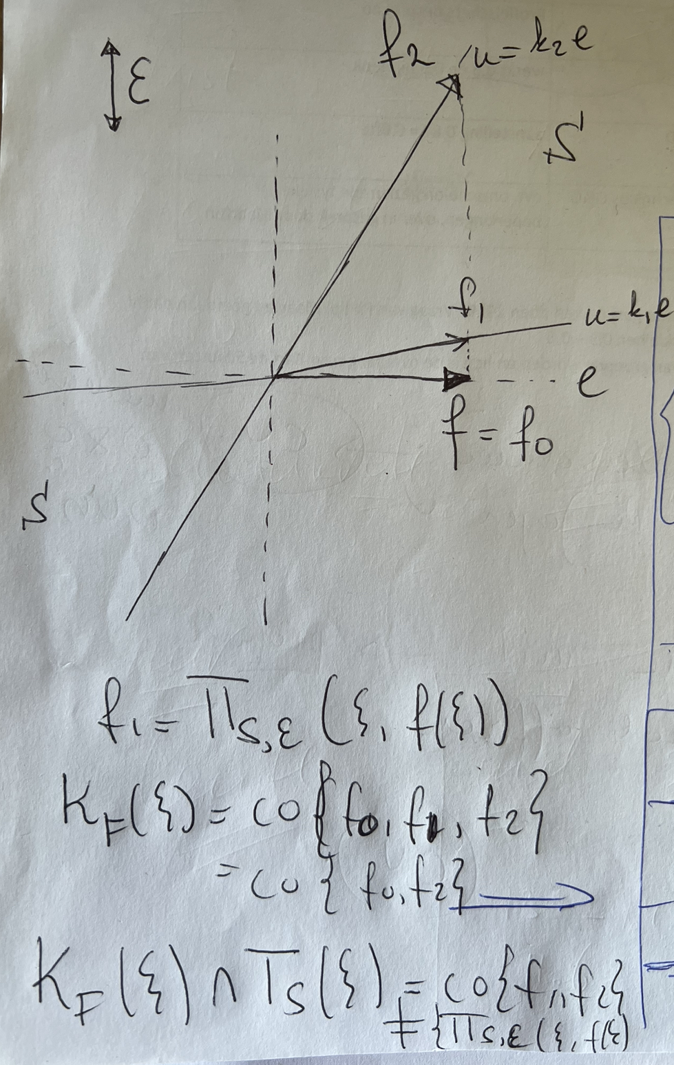
Figure 1: Due to the absence of convexity/prox regularity, we do not have that $K_{F}(\xi)\cap T_{\mathcal{S}}(\xi)=\{\Pi_{{\mathcal{S}},{\cal E}}(\xi,f(\xi))\}$. This is due to the tangent cone lacking a lower semicontinuity property (in the set ${\mathcal{K}}\cap-{\mathcal{K}}$.)

VII-F Corollaries

Corollary 16.

under lipschitz like bounds, we can prove global existence, i.e. on $[0,\infty)$ solutions

Proof.

concatenate, using lipschitz like bounds to avoid finite escape times. ∎

Corollary 17.

case of continuous inputs

Proof.

embed $t$ in it $\dot{t}=1$ and then for continuous input ∎

Corollary 18.

piecewise continuous inputs, make global results

Proof.

use previous corollary and concatenate, indicating that at continuities of $w$ you still are in the set $S$! so you can continue with a local solution, and as long as finite escape times are avoided we should be fine ∎

VIII Toulouse 20230206

VIII-A Extended PDS: Different facets of minimum norm formulation

The objective of this section is to write several analogues of extended PDS vector field which are similar to some known modeling formalism in the literature.

For given functions $h_{i}:\mathbb{R}^{n}\to\mathbb{R}$, $i=1,\dots,m$, we take $S$ to be of the following form:

$$S:=\{x\in\mathbb{R}^{n}\,|\,h_{i}(x)\geq 0\}.$$

The functions $h_{i}$, $i=1,\dots,m$ are smooth and that $\nabla h_{i}$ does not vanish in a neighborhood of $\{x\in\mathbb{R}^{n}\,|\,h_{i}(x)=0\}$. For all $x\in\mathbb{R}^{n}$, we define the set of active constraints at $x$ by

$$J(x)=\{i\in\{1,\dots,m\};h_{i}(x)\leq 0\}$$

The tangent cone to $S$ at $x$ is given by

$$T_{S}(x)=\{v\in R^{n}\,|\,\langle\nabla h_{i}(x),v\rangle\geq 0,i\in J(x)\}$$

and for $x\in S$, the normal cone is defined as

$$N_{S}(x)=\left\{\sum_{i\in J(x)}\lambda_{i}\nabla h_{i}(x),\lambda_{i}\leq 0\right\}$$

For a vector $f\in\mathbb{R}^{n}$, and a matrix $E$ with ${\mathcal{E}}={\rm im}\,E$, we consider

$$\Pi_{S,E}(x,f)=\operatorname{argmin}_{v\in T_{S}(x),v-f\in{\mathcal{E}}}\|v-f\|$$

We will now rewrite $\Pi_{S,E}(x,f)$ in terms of complementarity relations involving $T_{S}(x)$ and $N_{S}(x)$.

Figure 2: Orthogonality between $v^{*}=\Pi_{S,E}(x,f)$ and $\eta^{*}$, where $\eta^{*}$ satisfies $v^{*}-f=E\eta^{*}$.

KintTnotPi Need to show that optimality (of minimum norm problem) implies cone-complementarity relations.

MAURICE: some stuff below, not relevant now. Just kept it, we might see use of it - copy paste then

IX Preliminaries and classical PDS

IX-A Preliminary definitions

polyhedral set : given by the intersection of a finite number of closed half-spaces

Let $G=[g_{1}\ g_{2}\ldots g_{m}]\in\ree^{n\times m}$ and $g_{i}$, $i=1,2,\ldots,m$ are the columns of $G$. Then $\operatorname{pos}G$ is the convex cone consisting of all positive combinations of the columns of $G$ given by

$$\operatorname{pos}G=\{\sum_{i=1}^{m}\alpha_{i}g_{i}\mid\alpha_{i}\geq 0i=1,2,\ldots,m\}$$

$T_{K}(x)$ tangent cone [give definition 5.1.1] when $K$ closed convex cone we have $T_{K}(x)=\operatorname{cl}\bigcup_{t>0}\frac{K-x}{t}$ (see Remark 5.2.2. in [Uru] III). In fact, it holds due to convexity that for $x\in K$

$$\frac{K-x}{t_{2}}\subseteq\frac{K-x}{t_{1}}\text{ when }0<t_{1}\leq t_{2}$$ (58)

projection on a set $S$

$$P_{S}(x)=\operatorname{argmin}_{s\in S}\|s-x\|$$ (59)

IX-B Project dynamical systems

To introduce the “classical” projected dynamical systems (PDSs), consider a differential equation given by

$$\dot{x}(t)=f(x(t))$$ (60)

in which $x(t)\in\ree^{n}$ denotes the state at time $t\in\ree_{\geq 0}$. There is a restriction on the state $x$ in the sense that $x(t)$ has to remain inside a set $S\subseteq\ree^{n}$, which in PDS is ensured by redirecting the vector field at the boundary of $S$. Formally, PDS are given for a continuous vector field $f:\ree^{n}\rightarrow f$ and set $S\subseteq\ree^{n}$ (with further additional conditions) by

$$\dot{x}=\Pi_{S}(x,f(x))$$ (61)

with

$$\Pi_{S}(x,v)=\operatorname{argmin}_{w\in T_{S}(x)}\|w-v\|$$ (62)

for $x\in S$ and $v\in\ree^{n}$.

An equivalent characterisation of $\Pi_{S}(x,v)$, see [Hiriart-Urr, prop. 5.3.5 ], is

$$\Pi_{S}(x,v)=\lim_{\delta\downarrow 0}\frac{P_{S}(x+\delta v)-x}{\delta}$$ (63)

when $S$ is a closed convex non-empty set. In fact, in many works on PDS [XXX] this definition is adopted.

X Extended projected dynamical systems

X-A Model representation

Let set $S\subseteq\ree^{n}$ be given such that $S$ is a non-empty closed convex set, on which we impose additional conditions later to obtain a well-posed system. We are interested in dynamical systems

$$\dot{x}(t)=f(x(t))$$ (64)

in which the state of the system has to reside inside the set $S$. In classical PDS, as recalled in Subsection IX-B, the latter is ensured by “projecting” the vector field on the (tangent cone of the) set $S$, cf. (61) and (62). This projection is along all possible directions of the state in the sense that it just takes the vector $\Pi_{S}(x,v)\in T_{S}(x)$ that is “closest” to $v$ irrespective of the direction $\Pi_{S}(x,v)-v$. So, it is allowed to alter the complete vector field and thus the velocities of all the states $x$ in (64). Clearly, if (64) is a closed-loop system in the sense of an interconnection of a physical plant and a controller (and thus the state $x$ consists of physical plant states $x_{p}$ and controller states $x_{c}$), one cannot project in all directions. Indeed, the physical state dynamics cannot be modified by straightforward projection. It is only possible to ”project” the controller ($x_{c}$-)dynamics and possibly a part of the plant states $x_{p}$-dynamics in which the control input appears explicitly. For an example on the HIGS, see Section XXX below. Hence, in contrast to PDS, we only have limited directions in order to “correct ” the vector field $f(x)$ at the boundary. To formalize, this we model the “correction / projection” direction by the image of a matrix $E\in\ree^{n\times n_{E}}$, which is assumed to have full column rank. Formally, we get

$$\dot{x}=\Pi_{S,E}(x,f(x))$$ (65)

with

$$\Pi_{S,E}(x,v)=\operatorname{argmin}_{w\in T_{S}(x),w-v\in\im E}\|w-v\|$$ (66)

for $x\in S$ and $v\in\ree^{n}$.

Hence, the projection $\Pi$ projects the direction $v$ at $x\in S$ onto the set of admissible velocities (tangent cone) along $\im E$ in such a way that the correction $w-v$ is minimal in norm. For these systems, we coin the term extended Projected Dynamical Systems (ePDS), as they include the classical PDS (61) as a special case by taking $\im E=\ree^{n}$.

X-B Well-posed projection operator $\Pi_{S,E}$

Clearly, we have to show that the introduced projection $\Pi_{S,E}(x,v)$ is well-defined in the sense that it provides a unique outcome for each $x\in S$ and each $v\in\ree^{n}$. As in the case of classical PDS, this requires conditions on the set $S$ and, in this case, also on $E$. Although we envision that we can work under more general conditions, for the sake of setting the scene in this paper and inspired by the application of the HIGS, we focus on the setting below. Future work includes relaxing these conditions.

Assumption 19.

The set $S\subseteq\ree^{n}$ and $E\in\ree^{n\times n_{E}}$ satisfy

• $S=K\cup-K$ in which $K$ is a convex polyhedral cone given by $K=\operatorname{pos}G+\im H$ in which the matrix $[G\ H]$ is square and has rank $n$

• $K\cap-K=\im G$

• $E$ full column rank

• $\im E\cap S=\{0\}$ and thus $S+\im E=\ree^{n}$

Note that $K$ can also be written as

$$\{x\in\ree^{n}\mid Fx\geq 0\}$$ (67)

for some matrix $F\in\ree^{n_{f}\times n}$ (which we assume to be of full rank)

We are particularly interested in this setup as it can describe sector conditions as are used in reset controllers and the HIGS, e.g. describing that input and output of a controller must have the same sign, and also appear in circle and Popov criteria for the analysis of Lur’e type of systems, see e.g. [Khalil, Yakubovic]

To prove the well-posedness of (66) observe first that

$$T_{S}(x)=\begin{cases}T_{K}(x),&\text{ when }x\in K\setminus-K\\ K\cup-K,&\text{ when }x\in K\cap-K\\ -T_{K}(x),&\text{ when }x\in-K\setminus K\end{cases}$$ (68)

[add expression of $T_{K}(x)=\{w\in\ree^{n}\mid F_{I(x)}w\geq 0\}$ where $I(x)=\{i\in\{1,2,\ldots,n_{f}\}\mid F_{i}x=0\}$ the set of active constraints at $x$

Note that we can rewrite (66) as

$$\Pi_{S,E}(x,v)=v+E\eta^{*}(x,v)$$ (69)

with

$$\eta^{*}(x,v)=\operatorname{argmin}_{\eta\in\Lambda(x,v)}\|E\eta\|$$ (70)

and

$$\Lambda(x,v)=\{\eta\in\ree^{n_{E}}\mid v+E\eta\in T_{S}(x)\}$$ (71)

Lemma 20.

Under Assumption 19, it holds for each $x\in S$ and each $v\in\ree^{n}$ that $\Lambda(x,v)$ is a non-empty closed polyhedral set.

Proof.

Let $x\in S$ and $v\in\ree^{n}$ be given. First note that due to $S+\im E=\ree^{n}$ it follows that $\Lambda(x,v)$ is non-empty.

Clearly, when $x\not\in K\cap-K$ it follows that $T_{S}(x)$, as given in (68), is a closed polyhedral cone and then also $\Lambda(x,v)$ is a polyhedral set. So, let us turn our attention to $x\not\in K\cap-K$ in which $T_{S}(x)=K\cup K$ and thus $\Lambda(x,v)=\{\eta\in\ree^{n_{E}}\mid v+E\eta\in K\cup-K\}$.

Claim: $v+E\eta\in K$ and $v+E\bar{\eta}\in-K$ implies that $\eta=\bar{\eta}$.

Note that the Claim would show that if there is $\eta$ with $v+E\eta\in K$ then $\Lambda(x,v)=\{\eta\in\ree^{n_{E}}\mid v+E\eta\in K\}$ (as any $\eta$ in $\{\eta\in\ree^{n_{E}}\mid v+E\eta\in-K\}$ would also be contained in $\{\eta\in\ree^{n_{E}}\mid v+E\eta\in K\}$, and similarly if there is $\bar{\eta}$ with $v+E\bar{\eta}\in-K$ then $\Lambda(x,v)=\{\eta\in\ree^{n_{E}}\mid v+E\eta\in-K\}$. As the sets $\{\eta\in\ree^{n_{E}}\mid v+E\eta\in K\}$ and $\{\eta\in\ree^{n_{E}}\mid v+E\eta\in-K\}$ are both closed polyhedral sets, so is $\Lambda(x,v)$.

To prove the claim, observe that due to $K$ being a convex cone and $-v-E\bar{\eta}\in K$, we get that

$$E(\eta-\bar{\eta})=(v+E\eta)-v-E\bar{\eta}\in K$$

Since $\im E\cap S=\{0\}$ and $E$ full column rank, this shows that $\eta=\bar{\eta}$ and the result follows. ∎

Due to the constraint set of (70) being a closed polyhedral set, and the square of the cost function of (69) is $\eta^{\top}E^{\top}E\eta$ is a quadratic positive definite function (as $E$ full column rank), a unique minimizer exists, showing the well-posedness of (69) and thus (66).

Remark 21.

In case $x(0)\not\in S$, we can use $x(0+)=P_{S,E}(x(0))$ to reset the state to a state inside $S$. Note that this reset only occurs at the initial time and not afterwards, as the state never leaves $S$ for time $t>0$.

XI Connecting to alternative PDS representations

As already indicated in Subsection LABEL:sec:pds, there is an equivalence between the definitions (LABEL:piS) and (63) under certain conditions on the set $S$. In this section, the objective to establish a similar equivalence for ePDS.

To do so, let us first introduce

$$P_{S,E}(x)=\operatorname{argmin}_{s\in S,s-x\in\im E}\|s-x\|$$ (72)

Clearly, we can rewrite (66) as

$$P_{S,E}(x)=\operatorname{argmin}_{s\in C_{x}}\|s-x\|\text{ with }C_{x}:=\{s\in S\mid s-x\in\im E\}$$ (73)

Note that, although this formulation resembles (LABEL:piS), the set $C_{x}=S\cap(x+\im E)$ is dependent on $x$, which is not the case in (LABEL:piS). Observe that $C_{x}$ is a non-empty closed and convex set, as can be seen from a similar reasoning as in the proof of Lemma 20. In fact, this yields that $C_{x}$ is equal to $\{s\in K\mid s-x\in\im E\}$ or $\{s\in-K\mid s-x\in\im E\}$ due to the following implication:

$$\left.\begin{array}[]{c}s-x\in\im E,\ s\in K\\ \bar{s}-x\in\im E,\ \bar{s}\in K\end{array}\right\}\text{ imply }s=\bar{s}$$

Hence, $P_{S,E}(x)=P_{K,E}(x)$ (if $x\in K+\im E$) or $P_{S,E}(x)=P_{-K,E}(x)$ (if $x\in-K+\im E)$ and thus $P_{S,E}(x)$ gives a unique outcome, see, e.g., the reasoning on page 116 of [Uru]. Note that based on Theorem 3.3.1 in [Uru] and using the previous observation, we have that $P_{S,E}(x)$ is characterised by the following variational inequalities: $s_{x}$ is equal to $P_{S,E}(x)$ if and only if

$$\langle x-s_{x},s-s_{x}\rangle\leq 0\text{ for all }s\in S\cap(x+\im E)$$ (74)

In line with (63) for classical PDS, we consider also

$$\tilde{\Pi}_{S,E}(x,v)=\lim_{\delta\downarrow 0}\frac{P_{S,E}(x+\delta v)-x}{\delta}$$ (75)

Theorem 22.

Assumption 19, it holds that $\tilde{\Pi}_{S,E}(x,v)=\Pi_{S,E}(x,v)$ for all $x\in S$ and $v\in\ree^{n}$

Proof.

Following the arguments of the proof of Prop. 5.3.5 in [Uru], we can obtain that $\frac{P_{S,E}(x+\delta v)-x}{\delta}$ is equal to $P_{\frac{S-x}{\delta},E}(v)$. Indeed, using the variational inequalities characterisation of projections, we have that (74) for $s_{\delta}:=P_{S,E}(x+\delta v)$ gives that

$$\langle x+\delta v-s_{\delta},s-s_{\delta}\rangle\leq 0\text{ for all }s\in S,\ s-(x+\delta v)\in\im E$$

Hence, straightforward algebraic manipulations give for $\delta>0$ that

$$\langle v-\frac{s_{\delta}-x}{\delta},\frac{s-x}{\delta}-\frac{s_{\delta}-x}{\delta}\rangle\leq 0\text{ for all }s\in S,\ s-(x+\delta v)\in\im E$$

and thus

$$\langle v-\tilde{s},\tilde{s}-\frac{s_{\delta}-x}{\delta}\rangle\leq 0\text{ for all }\tilde{s}\in\frac{S-x}{\delta},\ \tilde{s}-v\in\im E$$

where we took $\tilde{s}=\frac{s-x}{\delta}$. From this we conclude indeed that $\frac{P_{S,E}(x+\delta v)-x}{\delta}=\frac{s_{\delta}-x}{\delta}=P_{\frac{S-x}{\delta},E}(v)$

Now we use that $T_{S}(x)=\lim_{\delta\downarrow 0}\frac{S-x}{\delta}$ (and the monotonicity of $\delta\mapsto\frac{S-x}{\delta}$ as in (58)) together with the fact that $\frac{S-x}{\delta}$ and the limit $T_{S}(x)$ are (the union of) convex closed sets, that $\tilde{\Pi}_{S,E}(x,v)=P_{T_{S}(x),E}(v)=\Pi_{S,E}(x,v)$. ∎