Stability and long-time behaviour of a rigid body containing a damper

Abstract

This paper provides a comprehensive analysis of stability and long-time behaviour of a coupled system constituted by two rigid bodies separated by a thin layer of lubricant. We show that permanent rotations of the whole system, with the solids at relative rest, are exponentially stable if and only if the axis of rotation is the principal axis of inertia corresponding to the largest moment of inertia of the outer body. All other equilibria are normally hyperbolic, and hence unstable. In addition, we show that all solutions to the governing equations converge to an equilibrium configuration, no matter which initial conditions are chosen. Numerical evidence of the above results as well as conditions ensuring attainability of the stable configurations are also presented.

For the stability analysis we use a linearization principle for dynamical systems possessing a center manifold. The characterization of the long-time behaviour is obtained by a careful analysis of the partially dissipative system of equations governing the motion of the coupled system.

MSC Classification]70K25,70E17,70E50,34A34,34D05,34D20

Declarations

Funding

Evan Arsenault gratefully acknowledges the support of the Natural Sciences and Engineering Research Council of Canada (NSERC) through the NSERC Undergraduate Student Research Award “Long-time dynamics of rigid bodies with a damper”.

Giusy Mazzone gratefully acknowledges the support of the Natural Sciences and Engineering Research Council of Canada (NSERC) through the NSERC Discovery Grant “Partially dissipative systems with applications to fluid-solid interaction problems”.

Conflicts of interest

The authors have no relevant financial or non-financial interests to disclose.

Availability of data and material

Not applicable.

Code availability

Not applicable.

Author’s contributions

All authors contributed to the investigations here reported. The first draft of the manuscript was written by Evan Arsenault and all authors commented on previous versions of the manuscript. All authors read and approved the final manuscript.

1 Introduction

Consider a system constituted by two rigid bodies $\mathcal{B}_{1}$ and $\mathcal{B}_{2}$, with $\mathcal{B}_{2}$ (strictly) contained in a spherical cavity within $\mathcal{B}_{1}$. The solids are separated only by a thin spherical layer of lubricant that completely fills the gap between the two solids (see Figure 1). We further assume that the inner solid $\mathcal{B}_{2}$ is a homogeneous spherical rigid body with radius $a\gg h$, where $h$ denotes the (constant) thickness of the gap between $\mathcal{B}_{2}$ and the surface of the cavity within $\mathcal{B}_{1}$.

\psfrag{1}{$\mathcal{B}_{1}$}\psfrag{2}{$\mathcal{B}_{2}$}\psfrag{G}{$G$}\psfrag{a}{$a$}\psfrag{h}{\footnotesize$h$}\includegraphics[width=238.49231pt]{rbd.eps}

Figure 1: A rigid body with a damper

In this paper, we consider the free rotations of the whole system about the center of mass $G$ of $\mathcal{B}_{1}$, i.e., we assume that there are no external forces acting on the system, and $G$ is a fixed point (see equation (2)). In addition, we ignore any translational motion of $\mathcal{B}_{2}$ within the cavity, and assume that the center $C$ of $\mathcal{B}_{2}$ coincides with $G$. We further suppose that the surface force (which is an internal force, due to the presence of the lubricant) between the two solids produces a torque which is proportional to the velocity of $\mathcal{B}_{2}$ relative to $\mathcal{B}_{1}$ (see equation (3)).

It is worth noticing that if there were no lubricant between the solids, then the motion of the two rigid bodies would be completely uncoupled (and thus, uninteresting). Furthermore, if there were no inner solid within the cavity, then the generic motion of the outer rigid body $\mathcal{B}_{1}$ would be a motion à la Poinsot. For example, depending on the initial conditions, $\mathcal{B}_{1}$ could perform a regular precession. Objective of this work is to show that the inner solid $\mathcal{B}_{2}$, subject to the type of torque described above (due to the lubricant), would stabilize the motion of the outer solid and take the whole system to a state (an equilibrium configuration, in fact, see Theorem 6) that is the relative rest of the solids with the whole system spinning with constant angular velocity around one of the principal axes of inertia of $\mathcal{B}_{1}$. In this sense (also inspired by chern ), we refer to $\mathcal{B}_{2}$ as the “damper”, and to the whole system as a “rigid body with a spherical damper”.

According to chern (see also (evo, , Section 7.4) and references therein), M.  A. Lavrentyev considered this problems as a lumped mass parameter system approximating the motion of a rigid body with a cavity filled with a viscous fluid. Chernous’ko (see, e.g., chern ; evo ), obtained conditions on physical quantities (like fluid density and viscosity) under which equations (6), describing the motions of a rigid body with a spherical damper, would as well describe the motion of a rigid body with a spherical cavity filled with an incompressible viscous fluid (at low Reynolds number). The motion of fluid-filled rigid bodies is studied in connection with geophysical applications in the search of sources for the geomagnetic field, in structural engineering for the design of tuned liquid dampers, as well as in space engineering for the stabilization of spacecrafts (see giu and references therein).

In chern ; evo , the authors derived necessary and sufficient conditions for the stability of permanent rotations of the system, as a whole rigid body, around one of the principal axis of inertia of the outer solid. Let us be more precise. Consider the equilibrium configuration which is characterized by $\mathcal{B}_{2}$ at relative rest with respect to $\mathcal{B}_{1}$, and the whole system of rigid body with a damper rotating with constant angular velocity $\Omega^{*}$ around the principal axes of inertia $\mathsf{a}$ of $\mathcal{B}_{1}$. Let $A$ be the corresponding principal moment of inertia of $\mathcal{B}_{1}$, and denote with $B$ and $C$ the remaining moments of inertia. Using a spectral stability argument, Chernous’ko et al. show that a necessary condition for the stability (in the sense of Lyapunov) of $\Omega^{*}$ is that $A\geq B,C$. In the same works, sufficient conditions are obtained using the classical Lyapunov method. It is then found that $\Omega^{*}$ is stable if $A>B,C$. These results are nonlinear stability results which are silent about the asymptotic stability properties of equilibria as well as the long-time behaviour of generic motions. For example, it is not known whether trajectories starting sufficiently close to $\Omega^{*}$ would eventually (as time goes to infinity) converge to an equilibrium, and if so, with what rate.

In this paper, we show that the condition $A\geq B,C$ is a necessary and sufficient condition for the stability of $\Omega^{*}$ (see Theorem 11), and we also prove that all trajectories corresponding to solutions of the equations of motion will converge to an equilibrium configuration at an exponential rate, no matter how one chooses the initial conditions (see Theorem 13). The stability results are obtained using a principle of linearized stability for autonomous systems of ordinary differential equations with normally stable and/or normally hyperbolic equilibria (see Definition 1, and Theorems 2 & 3). A spectral analysis of the equations of motion (6) shows that equilibria are, indeed, either normally stable or normally hyperbolic (see Theorem 10). The long-time behaviour of generic motions $z(t\mathchar 24635\relax\;z_{0})$ is obtained by showing that the corresponding $\omega$-limit set $\omega(z_{0})$ is non-empty, compact and connected, it is made of either only normally stable equilibria or only normally hyperbolic ones, and

$$\lim_{t\rightarrow\infty}\text{d}(z(t\mathchar 24635\relax\;z_{0}),\omega(z_{0}))=0.$$

Convergence to an equilibrium point is then a consequence of the asymptotic stability properties of normally stable and normally hyperbolic equilibria according to Theorems 2 & 3.

This paper also provides sufficient conditions on the attainability of the stable equilibrium configurations. In addition, we present some results concerning the numerical approximation of solutions to (6). These results provide further insights on the stability conditions as well as on the attainability of equilibria.

Beside their novelty, the results of this paper are non-trivial considering that the equations of motion are only partially dissipative. In fact, even if the total kinetic energy of the whole system decreases along the trajectories, the two solids must move while keeping the total angular momentum conserved at all times (see Proposition 4). In particular, neither the balance of kinetic energy (8), nor the Lyapunov function constructed in chern ; evo could directly provide a decay with rate for the relative velocity of the solids. We show that an exponential decay of the solids relative velocity happens after “some time” the system has been moving, see Theorem 13 and the numerical results in Figures 3 & 4. Another point of interest is the way we prove the spectral stability properties of our equilibria which differs from that in chern ; evo , and it has a more geometrical flavour as it shows how the spectrum of the linearization moves while changing the ordering of the moment of inertia of $\mathcal{B}_{1}$ (see proof of Theorem 10). We believe that such a complete and rigorous analytical treatment could be beneficial in the analysis of similar problems in rigid body dynamics involving the design of dampening mechanisms.

Finally, this paper is in line with the recent work of the second author and collaborators concerning the stabilization of rigid bodies (DiGaMaZu ; MaPrSi ; MaPrSi19 ; giu2 ). In particular, in giu2 , the second author of this paper has investigated the existence of solutions, and provided a preliminary analysis of the long-time behaviour of generic trajectories for the (more complete) fluid-solid interaction problem of rigid bodies separated by a gap filled by a viscous incompressible fluid (obeying the Navier-Stokes equations). In this respect, the current work could provide some insights for the study of stability and long-time behaviour of the physical system considered in giu2 .

Here is the plan of the paper. We begin with Section 2 containing some notation and the general stability theorems for autonomous systems that we will use for our physical problem. In Section 3, we derive the equations governing the motion of a rigid body with a damper, and we provide preliminary properties of their solutions (like global existence, uniqueness, and energy balances). In Section 4, we provide a linear and nonlinear stability analysis of the equilibria. The long-time behaviour of generic trajectories is completely characterized in Section 5. Numerical evidence of the above results is provided in Section 6.

2 Notation and useful results

We use the symbol $\left\lVert\cdot\right\rVert$ for the Euclidean norm in the $d$-dimensional Euclidean space $\mathbb{R}^{d}$, and denote with $\langle\cdot,\cdot\rangle$ the standard dot product in $\mathbb{R}^{d}$. We recall that $\left\lVert u\right\rVert=\sqrt{\langle u,u\rangle}$ for every $u\in\mathbb{R}^{d}$. In addition, for $r>0$ and $x_{0}\in\mathbb{R}^{d}$, $B_{r}(x_{0})$ denotes the open ball centered at $x_{0}$ and with radius $r$, i.e.,

$$B_{r}(x_{0}):=\{x\in\mathbb{R}^{d}:\;\left\lVert x-x_{0}\right\rVert<r\}.$$

Similarly,

$$\overline{B_{r}}(x_{0}):=\{x\in\mathbb{R}^{d}:\;\left\lVert x-x_{0}\right\rVert\leq r\}$$

denotes the closed ball centered at $x_{0}$ and with radius $r$.

In $\mathbb{C}^{d}$, we consider the inner product (over the field $\mathbb{C}$)

$$\langle z,w\rangle_{\mathbb{C}^{d}}:=\langle z,\overline{w}\rangle\\ \quad=\langle\mathsf{Re}(z),\mathsf{Re}(w)\rangle+\langle\mathsf{Im}(z),\mathsf{Im}(w)\rangle+i\left(\langle\mathsf{Im}(z),\mathsf{Re}(w)\rangle-\langle\mathsf{Re}(z),\mathsf{Im}(w)\rangle\right),$$

and associated norm $\left\lVert z\right\rVert_{\mathbb{C}^{d}}=\sqrt{\langle z,z\rangle_{\mathbb{C}^{d}}}=\sqrt{(\mathsf{Re}(z))^{2}+(\mathsf{Im}(z))^{2}}$. In the above, we have denoted with $\mathsf{Re}(\cdot)$ and $\mathsf{Im}(\cdot)$ the real and imaginary part of a complex number, respectively.

For a matrix $A\in\mathbb{R}^{d\times d}$, $\sigma(A)$ denotes the spectrum of $A$, i.e.,

$$\sigma(A)=\{\lambda\in\mathbb{C}:\;\text{there exists }u\in\mathbb{R}^{d}\setminus\{0\}\text{ such that }Au=\lambda u\}.$$

$A^{T}$ denotes the transpose of $A$. $\mathsf{SO}(3)$ denotes the special orthogonal group of all orthogonal matrices with determinant 1. We recall that for a skew-symmetric matrix $A\in\mathbb{R}^{d\times d}$ (i.e., $A^{T}=-A$), there exists a vector $\alpha\in\mathbb{R}^{d}$ (called axial vector) such that $Av=\alpha\times v$ for every $v\in\mathbb{R}^{d}$.

This paper makes use of the following useful results, the first being a modified Gronwall lemma.

Lemma 1.

Suppose that a function $y\in L^{\infty}(0,\infty),y\geq 0$, satisfies the following inequality for all $t\geq 0$:

$$\dot{y}(t)\leq-Cy(t)+F(t),$$

where $C>0$ is a constant, and $F\in L^{q}(a,\infty)\cap L^{1}_{\text{loc}}(0,\infty)$, for some $a>0$ and $q\in[1,\infty)$, satisfies $F(t)\geq 0$ for a. a. $t\geq 0$. Then:

$$\lim_{t\rightarrow\infty}y(t)=0$$

If $F\equiv 0$, then:

$$y(t)\leq y(0)e^{-Ct},\quad\text{for all }t\geq 0.$$

In the above $L^{q}(a,b)$, with $q\in[1,\infty]$, identifies the usual Lebesgue space of real-valued functions defined on the interval $(a,b)$, with $-\infty\leq a<b\leq+\infty$. A proof of the above lemma can be found in giu .

Next, we will also consider the functional space $C^{1}(D,\mathbb{R}^{d})$ of all continuously differentiable functions from an open subset $D\subset\mathbb{R}^{d}$ to $\mathbb{R}^{d}$. For the stability analysis, we will need the following notions from (pruss, , Chapter 10).

Definition 1 (Normally Stable and Normally Hyperbolic Equilibria).

Let $D\subset\mathbb{R}^{d}$ be an open set and $f\in C^{1}(D,\mathbb{R}^{d})$. Consider the nonlinear system of ordinary differential equations (ODEs)

$$\dot{z}=f(z).$$ (1)

Let $\mathcal{E}\subset D$ denote the set of equilibrium points for (1), i.e., $z\in\mathcal{E}$ if and only if $f(z)=0$. For $z^{*}\in\mathcal{E}$ we assume that the following conditions are satisfied:

1. Near $z^{*}$, $\mathcal{E}$ forms a $C^{1}$-manifold of dimension $0<m\leq d$. This means that there exists an open set $U\subset\mathbb{R}^{m}$, $0\in U$, and there exists a function $\psi:\;U\to\mathbb{R}^{d}$ such that $\psi(U)\subset\mathcal{E}$, $\psi(0)=z^{*}$, and $\text{Rank }\psi^{\prime}(0)=m$, where $\psi^{\prime}(0)\in\mathbb{R}^{m\times m}$ denotes the Jacobian matrix of $\psi$ at $0$.

2. $T_{z^{*}}\mathcal{E}=N(A)$, where $T_{z^{*}}\mathcal{E}$ denotes the tangent space of $\mathcal{E}$ at $z^{*}$, $A:=f^{\prime}(z^{*})$ is the Fréchet derivative of $f$ at $z^{*}$, and $N(A)$ is the null space of $A$. We may sometimes refer to $A$ as the linearization near the equilibrium $z^{*}$.

3. $\lambda=0$ is a semi-simple eigenvalue of $A$, i.e., $N(A^{2})=N(A)$.

4. $\sigma(A)\cap i\mathbb{R}=\{0\}$.

Then, the following two definitions holds:

1. $z^{*}$ is said to be normally stable if $\sigma(A)\setminus\{0\}\subset\mathbb{C}^{-}$, where $\mathbb{C}^{-}:=\{\lambda\in\mathbb{C}:\;\mathsf{Re}(\lambda)<0\}$.

2. $z^{*}$ is said to be normally hyperbolic if $\sigma(A)\cap\mathbb{C}^{-}\neq\varnothing$ and $\sigma(A)\cap\mathbb{C}^{+}\neq\varnothing$, where $\mathbb{C}^{+}:=\{\lambda\in\mathbb{C}:\;\mathsf{Re}(\lambda)>0\}$.

Remark 1.

Geometrically, the condition in the definition of semi-simple eigenvalue is equivalent to requiring that the algebraic and geometric multiplicities of the eigenvalue $\lambda=0$ must coincide.

While for linear systems, we could take conditions (i) and (ii) as definition of stable and unstable equilibrium, respectively, for nonlinear systems of ODEs we will consider the following more general definition of stability due to Lyapunov.

Definition 2 (Stability in the sense of Lyapunov).

Let $t_{0}\geq 0$. An equilibrium point $z^{*}$ of (1) is said to be stable (in the sense of Lyapunov) if for every $\varepsilon>0$, there exists $\delta=\delta(\varepsilon)>0$ such that for any $z_{0}\in G$ satisfying the condition $\|z_{0}-z^{*}\|\leq\delta$, the (unique) solution to the initial value problem

$$\dot{z}=f(z),\qquad z(t_{0})=z_{0}$$

satisfies $\|z(t)-z^{*}\|<\varepsilon$ for every $t\geq t_{0}$.

The equilibrium point $z^{*}$ of (1) is said to be unstable if it is not stable (in the sense of Lyapunov).

The following linearization principles hold.

Theorem 2.

Consider the nonlinear system of ODEs (1), and assume that $z^{*}$ is normally stable. Then, the equilibrium $z^{*}$ is stable (in the sense of Lyapunov) and there exists $\delta>0$ such that the unique solution to the initial value problem

$$\dot{z}=f(z),\qquad z(0)=z_{0}$$

with $z_{0}\in B_{\delta}(z^{*})$ exists for all $t\geq 0$. Moreover, there exist $z_{\infty}\in\mathcal{E}$ and constants $c_{1},\;c_{2}>0$ such that:

$$\left\lVert z(t)-z_{\infty}\right\rVert\leq c_{1}e^{-c_{2}t}$$

for all $t\geq 0$.

For a proof, we refer to (pruss, , Satz 10.4.1)

Theorem 3.

Consider the nonlinear system of ODEs (1), and assume that $z^{*}$ is normally hyperbolic. Then the equilibrium $z^{*}$ is unstable.

Furthermore, for every sufficiently small $\rho>0$ there is a $\delta\in(0,\rho]$, such that the solution $z(t)$ with initial value $z_{0}\in B_{\delta}(z^{*})$ satisfies exactly one of the following two properties:

• $d(z(t^{*}),\mathcal{E}):=\inf_{z^{*}\in\mathcal{E}}\left\lVert z(t^{*})-z^{*}\right\rVert>\rho$ for some $t^{*}>0$;

• $z(t)$ is globally defined for all $t\geq 0$, and there exist $z_{\infty}\in\mathcal{E}$ and constants $c_{1},\;c_{2}>0$ such that: $\left\lVert z(t)-z_{\infty}\right\rVert\leq c_{1}e^{-c_{2}t}$ for all $t\geq 0$.

A proof of this theorem can be found in (pruss, , Satz 10.5.1).

Remark 2.

The above two theorems are generalizations of classical linearization principles for almost linear systems of ODEs, to the case in which the linearization $A$ has zero as eigenvalue (cf. (boyce, , Section 9.3)).

3 Equations of motion

We fix an inertial frame $\Sigma_{s}$ and a body frame $\Sigma_{b}:=\{G\mathchar 24635\relax\;\mathsf{a}_{1},\mathsf{a}_{2},\mathsf{a}_{3}\}$ both with origin at $G$, and $\Sigma_{b}$ having axes directed along the (orthonormal basis of) eigenvectors of the inertia tensor $J$ of $\mathcal{B}_{1}$ with respect to $G$ (these axes are called principal axes of inertia). We denote $A_{1}$, $A_{2}$, $A_{3}$ the corresponding (positive) eigenvalues of $J$ (called principal moments of inertia of $\mathcal{B}_{1}$), and we assume that $A_{1}\leq A_{2}\leq A_{3}$. The inner body $\mathcal{B}_{2}$ has inertia tensor $I\mathbf{E_{0}}$ relative to $G$, where $\mathbf{E_{0}}$ is the identity tensor. Thus, $J_{c}:=J+I\mathbf{E_{0}}$ denotes the inertia tensor (with respect to the center of mass $G$) of the whole system of rigid body with spherical damper.

Let $\omega$ and $\omega_{1}$ be the angular velocities of $\mathcal{B}_{1}$ and $\mathcal{B}_{2}$ in the frame $\Sigma_{s}$, respectively. Similarly, we denote with $\Omega$ and $\Omega_{1}$ the angular velocities of the outer and inner bodies in the frame $\Sigma_{b}$, respectively.

We assume that the interaction between the solids is described by viscous forces (due to the presence of the lubricant) that produce a total torque (relative to $G$) on $\mathcal{B}_{1}$ of the form $T:=k(\omega_{1}-\omega)$ in $\Sigma_{s}$, with $k$ a positive constant depending on the lubricant density, viscosity and thickness $h$, and on the damper radius $a$ (see (chern, , Equation (8.6))).

We begin with the following balances of angular momentum in the inertial frame $\Sigma_{s}$

$$\frac{dm_{total}}{dt} =0,$$ (2)

$$\frac{dm_{inner}}{dt} =-k(\omega_{1}-\omega).$$ (3)

In the two above equations, $m_{total}$ and $m_{inner}$ are the total angular momentum and the angular momentum of the inner body $\mathcal{B}_{2}$ calculated with respect to $G$, respectively.

Given the time dependence of the volumes $\mathcal{B}_{1}$ (and thus of the inertia tensor of $\mathcal{B}_{1}$) in $\Sigma_{s}$, it is more convenient to rewrite the above equations of motion in the moving frame $\Sigma_{b}$. In such a frame, $J=\text{diag}(A_{1},A_{2},A_{3})$. We then note that $\Omega=R^{T}\omega$ and $\Omega_{1}=R^{T}\omega_{1}$ for some $R=R(t)\in\mathsf{SO}(3)$ for all $t\geq 0$, with $R(0)=\bf{E}_{0}$. Note that $\Omega$ is the axial vector of $R^{T}\dot{R}$, i.e., $R^{T}\dot{R}u=\Omega\times u$ for every $u\in\mathbb{R}^{3}$. In the body frame $\Sigma_{b}$, the total angular momentum $M_{total}$ is

$$M_{total}:=R^{T}m_{total}=J\Omega+I\Omega_{1}$$

The balance of angular momentum in the body frame $\Sigma_{b}$ then becomes

$$J\dot{\Omega}+\Omega\times(J\Omega)+I\dot{\Omega}_{1}+\Omega\times(I\Omega_{1})=0.$$ (4)

The inner body is spherical and hence its inertia tensor about the center of mass is just $I\mathbf{E_{0}}$ (constant) regardless of frame. Since $\omega=R\Omega,\omega_{1}=R\Omega_{1}$, the previous equation can be rewritten as follows

$$I\dot{\Omega}_{1}+\Omega\times(I\Omega_{1})=-k(\Omega_{1}-\Omega).$$ (5)

Subtracting (5) from (4) and collecting the two gives the following system of equations describing the motion of a rigid body with a damper in the moving frame $\Sigma_{b}$:

$$\begin{split}J\dot{\Omega}+\Omega\times(J\Omega)&=k(\Omega_{1}-\Omega),\\ I\dot{\Omega}_{1}+\Omega\times(I\Omega_{1})&=-k(\Omega_{1}-\Omega).\end{split}$$

Since $J$ is a positive definite tensor, we invert $J$ to get the following system of differential equations governing the motion of the rigid body $\mathcal{B}_{1}$ with the spherical damper $\mathcal{B}_{2}$

$$\begin{cases}\dot{\Omega}=J^{-1}(k(\Omega_{1}-\Omega)-\Omega\times(J\Omega)),\\ \dot{\Omega}_{1}=\displaystyle-\frac{k}{I}(\Omega_{1}-\Omega)-\Omega\times\Omega_{1}.\end{cases}$$ (6)

Consider the function $F:\mathbb{R}^{3}\times\mathbb{R}^{3}\to\mathbb{R}^{6}$ such that

$$\qquad F(\Omega,\Omega_{1}):=\left[\begin{matrix}J^{-1}(k(\Omega_{1}-\Omega)-\Omega\times(J\Omega))\\ \displaystyle-\frac{k}{I}(\Omega_{1}-\Omega)-\Omega\times\Omega_{1}\end{matrix}\right].$$ (7)

Since $F$ is continuously differentiable in $\mathbb{R}^{3}\times\mathbb{R}^{3}$, for any initial data $(\Omega_{0},\Omega_{10})\in\mathbb{R}^{3}\times\mathbb{R}^{3}$, the initial value problem

$$\frac{d}{dt}\left[\begin{matrix}\Omega\\ \Omega_{1}\end{matrix}\right]=F(\Omega,\Omega_{1}),\qquad\left[\begin{matrix}\Omega(0)\\ \Omega_{1}(0)\end{matrix}\right]=\left[\begin{matrix}\Omega_{0}\\ \Omega_{10}\end{matrix}\right]$$

has a unique solution defined on the maximal existence interval $[0,t_{+})$ for some $t_{+}=t_{+}(\Omega_{0},\Omega_{10})>0$. We will soon see that $t_{+}=+\infty$. While we cannot explicitly solve (6) in all cases, we can derive some useful properties of the solutions to (6) like the balances of the kinetic energy and total angular momentum.

First consider the kinetic energy, defined by

$$V(\Omega,\Omega_{1}):=\frac{1}{2}(\langle\Omega,J\Omega\rangle+I\langle\Omega_{1},\Omega_{1}\rangle).$$

By taking the time derivative of $V$ and using equations (6), we get

$$\frac{dV}{dt} =\frac{1}{2}(2\langle\Omega,J\dot{\Omega}\rangle+2I\langle\Omega_{1},\dot{\Omega}_{1}\rangle)$$

$$=\langle\Omega,k(\Omega_{1}-\Omega)-\Omega\times(J\Omega)\rangle+\langle\Omega_{1},-k(\Omega_{1}-\Omega)-I(\Omega\times\Omega_{1})\rangle$$

$$=-k\left\lVert\Omega_{1}-\Omega\right\rVert^{2}.$$

Hence the rate of change of the kinetic energy along the solutions of (6) reads as follows

$$\frac{d}{dt}V(\Omega(t),\Omega_{1}(t))=-k\left\lVert\Omega_{1}(t)-\Omega(t)\right\rVert^{2}.$$ (8)

The above equation physically expresses the balance of the kinetic energy of the whole system.

Another important balance is that of the angular momentum. Consider the quantity $K^{2}=K^{2}(\Omega,\Omega_{1}):=\left\lVert J\Omega+I\Omega_{1}\right\rVert^{2}$. By taking the time derivative of $K^{2}$ we get the following equation:

$$\frac{dK^{2}}{dt} =2\langle J\Omega+I\Omega_{1},J\dot{\Omega}+I\dot{\Omega}_{1}\rangle$$

$$=2\langle J\Omega+I\Omega_{1},k(\Omega_{1}-\Omega)-\Omega\times(J\Omega)-k(\Omega_{1}-\Omega)-I(\Omega\times\Omega_{1})\rangle$$

$$=-2\langle J\Omega+I\Omega_{1},\Omega\times(J\Omega+I\Omega_{1})\rangle$$

$$=0.$$ (9)

Thus the quantity $K^{2}$ is constant along solutions of (6). We summarize the above results in the next proposition.

Proposition 4.

Let $(\Omega,\Omega_{1})$ be a solution to the system of ODEs (6). Then,

• $(\Omega,\Omega_{1})$ satisfies (8).

• $(\Omega,\Omega_{1})$ satisfies (9).

Since $J$ is positive definite and $I$ is a positive constant, a corollary of the statement (i) is that the functions $\Omega(t),\Omega_{1}(t)$ are uniformly bounded for all $t\geq 0$, and by the classical continuation theorem for ODEs (see (coddington, , Theorem 4.1)), it follows that $t_{+}=+\infty$. In addition, Proposition 4(ii) allows us to define invariant sets for all solutions of (6). Indeed, for a given initial condition $(\Omega_{0},\Omega_{10})$, let $M=K^{2}(\Omega_{0},\Omega_{10})$ and define the set $A(M)$:

$$A(M)=\{(\omega,\omega_{1})\in\mathbb{R}^{6}:K^{2}(\omega,\omega_{1})=M\}$$

Then the solution to (6) corresponding to $(\Omega_{0},\Omega_{10})$ must stay within $A(M)$ for all times. Furthermore, since $K^{2}$ is a continuous function and $A(M)$ is the preimage of a compact set in $\mathbb{R}^{6}$, we have the following property.

Lemma 5.

The set $A(M)$ is compact.

4 Equilibria and their stability properties

4.1 Equilibria

We begin this section by characterizing the equilibria of (6) in the following theorem, first proved in evo .

Theorem 6.

The point $(\Omega^{*},\Omega_{1}^{*})\in\mathbb{R}^{3}\times\mathbb{R}^{3}$ is an equilibrium point of (6) if and only if $\Omega^{*}=\Omega_{1}^{*}$ and $\Omega^{*}$ is either the zero vector in $\mathbb{R}^{3}$ or an eigenvector of $J$.

Proof: Assume that $F(\Omega^{*},\Omega_{1}^{*})=0$, then from (6) we have:

$$\begin{cases}\Omega^{*}\times(J\Omega^{*})=k(\Omega_{1}^{*}-\Omega^{*})\\ \Omega^{*}\times(I\Omega_{1}^{*})=-k(\Omega_{1}^{*}-\Omega^{*})\end{cases}$$

Taking the dot product of both sides of the second equation by $(\Omega_{1}^{*}-\Omega^{*})$, it gives $-k\left\lVert\Omega_{1}^{*}-\Omega^{*}\right\rVert^{2}=0$, and thus we must have $\Omega^{*}=\Omega_{1}^{*}$. Replacing the latter in the first equation of the above system, it follows that $\Omega^{*}\times(J\Omega^{*})=0$ which holds if and only if $\Omega^{*}$ is either the zero vector in $\mathbb{R}^{3}$ or an eigenvector of $J$.

The converse implication is trivially true.

Remark 3.

Define $\{\mathbf{e}_{i}\}_{i=1}^{6}$ to be the standard basis vectors of $\mathbb{R}^{6}$. From our assumption that $A_{1}\leq A_{2}\leq A_{3}$, there are four possible cases for the set of equilibria $\mathcal{E}$:

1. $A_{1}<A_{2}<A_{3}\implies\mathcal{E}=\text{span}\{\mathbf{e}_{1}+\mathbf{e}_{4}\}\cup\text{span}\{\mathbf{e}_{2}+\mathbf{e}_{5}\}\cup\text{span}\{\mathbf{e}_{3}+\mathbf{e}_{6}\}$

2. $A_{1}=A_{2}<A_{3}\implies\mathcal{E}=\text{span}\{\mathbf{e}_{1}+\mathbf{e}_{4},\mathbf{e}_{2}+\mathbf{e}_{5}\}\cup\text{span}\{\mathbf{e}_{3}+\mathbf{e}_{6}\}$

3. $A_{1}<A_{2}=A_{3}\implies\mathcal{E}=\text{span}\{\mathbf{e}_{1}+\mathbf{e}_{4}\}\cup\text{span}\{\mathbf{e}_{2}+\mathbf{e}_{5},\mathbf{e}_{3}+\mathbf{e}_{6}\}$

4. $A_{1}=A_{2}=A_{3}\implies\mathcal{E}=\text{span}\{\mathbf{e}_{1}+\mathbf{e}_{4},\mathbf{e}_{2}+\mathbf{e}_{5},\mathbf{e}_{3}+\mathbf{e}_{6}\}$

4.2 Nonlinear stability

For the study of the stability, we will use the linearization principles in Theorem 2 and Theorem 3. Let us start by linearizing the equations (6) around a (nonzero) equilibrium $(\Omega^{*},\Omega_{1}^{*}\equiv\Omega^{*})$. By Theorem 6 there exists $\lambda^{*}\in\{A_{1},A_{2},A_{3}\}$ such that $(J-\lambda^{*}\mathbf{E_{0}})\Omega^{*}=0$. We will also denote $\mathsf{eigen}_{J}(\lambda^{*})$ the eigenspace corresponding to the eigenvalue $\lambda^{*}$ of $J$.

For every $(\Omega,\Omega_{1})\in\mathbb{R}^{6}$, the Gateaux derivative of $F$ at $(\Omega^{*},\Omega_{1}^{*}\equiv\Omega^{*})$ is given by

$$\begin{split}\frac{d}{dt}&F(\Omega^{*}+t\Omega,\Omega_{1}^{*}+t\Omega_{1})|_{t=0}\\ &=\left[\begin{matrix}J^{-1}(k(\Omega_{1}-\Omega)-\Omega^{*}\times(J-\lambda^{*}\mathbf{E_{0}})\Omega)\\ -k/I(\Omega_{1}-\Omega)-\Omega^{*}\times(\Omega_{1}-\Omega)\end{matrix}\right]=L^{*}\left[\begin{matrix}\Omega\\ \Omega_{1}\end{matrix}\right],\end{split}$$ (10)

for some linear transformation $L^{*}=L^{*}(J,k,I,\Omega^{*},\Omega^{*}_{1}):\;\mathbb{R}^{3}\times\mathbb{R}^{3}\to\mathbb{R}^{3}\times\mathbb{R}^{3}$. We will refer to $L^{*}$ as the linearization at the equilibrium $(\Omega^{*},\Omega_{1}^{*}\equiv\Omega^{*})$.

The rest of this section concerns the above linear transformation. We start with the following lemma asserting that the null space of $L^{*}$ is characterized by equilibria.

Lemma 7.

$N(L^{*})=\{v=(\Omega,\Omega_{1})\in\mathcal{E}:\;\Omega=\Omega_{1}\in\mathsf{eigen}_{J}(\lambda^{*})\}$.

Proof: Let $v=(\Omega,\Omega_{1})\in\mathbb{R}^{3}\times\mathbb{R}^{3}$ be such that $L^{*}v=0$. From (10), the condition $L^{*}v=0$ is equivalent to the following system of equations:

$$\begin{split}&k(\Omega_{1}-\Omega)-\Omega^{*}\times(J-\lambda^{*}\mathbf{E_{0}})\Omega=0,\\ &-\frac{k}{I}(\Omega_{1}-\Omega)-\Omega^{*}\times(\Omega_{1}-\Omega)=0.\end{split}$$ (11)

Dot multiplying both sides of the second equation by $\Omega-\Omega_{1}$, we find that $\left\lVert\Omega-\Omega_{1}\right\rVert=0$, thus implying that $\Omega=\Omega_{1}$. As a consequence, the first equation of the above system nows reads

$$\Omega^{*}\times[(J-\lambda^{*}\mathbf{E_{0}})\Omega]=0,$$

and we can infer the existence of a scalar $\bar{\lambda}\in\mathbb{R}$ such that

$$(J-\lambda^{*}\mathbf{E_{0}})\Omega=\bar{\lambda}\Omega^{*}.$$

Let us take the dot product of the latter displayed equation by $\Omega^{*}$ and we find that

$$\bar{\lambda}\left\lVert\Omega^{*}\right\rVert^{2}=\langle\Omega,J\Omega^{*}\rangle-\lambda^{*}\langle\Omega,\Omega^{*}\rangle=0.$$

Thus, $\bar{\lambda}=0$ and we can conclude that also $(J-\lambda^{*}\mathbf{E_{0}})\Omega=0$.

Summarizing, we have shown that $v=(\Omega,\Omega_{1})\in N(L^{*})$ satisfies $\Omega=\Omega_{1}$ and $(J-\lambda^{*}\mathbf{E_{0}})\Omega=0$. Hence, by Theorem 6, we conclude that $v=(\Omega,\Omega_{1})\in\mathcal{E}$ with $\Omega=\Omega_{1}\in\mathsf{eigen}_{J}(\lambda^{*})$.

The converse inclusion is immediately verified.

Due to the presence of the zero eigenvalue, we cannot apply the classical linearization principles for almost linear systems (see (boyce, , Section 9.3)). This motivates our attempt to use Theorem 2 and Theorem 3 instead. The remainder of this section focuses on verifying that our equilibria satisfy the conditions of those theorems, starting with the following lemmas.

Lemma 8.

$\sigma(L^{*})\cap i\mathbb{R}=\{0\}$.

Proof: This proof requires verifying that in all cases we cannot have a purely imaginary eigenvalue. Given (10), an equivalent proof of the above statement is to show that the following linear system of ODEs

$$\begin{split}J\dot{\Omega}&=k(\Omega_{1}-\Omega)-\Omega^{*}\times(J-\lambda^{*}\mathbf{E_{0}})\Omega\\ I\dot{\Omega}_{1}&=-k(\Omega_{1}-\Omega)-I\Omega^{*}\times(\Omega_{1}-\Omega)\end{split}$$ (12)

does not admit any periodic solution other than the trivial one. Let us argue by contradiction, and assume that the above system of ODEs admits a nontrivial periodic solution $(\Omega,\Omega_{1})$ with period $T>0$ (i.e., $(\Omega(t),\Omega_{1}(t))=(\Omega(t+T),\Omega_{1}(t+T))$ for every $t\in\mathbb{R}$). Without loss of generality, we will assume that

$$\int^{T}_{0}\Omega(t)\;dt=0,\qquad\int^{T}_{0}\Omega_{1}(t)\;dt=0.$$ (13)

Let us denote $K:=J\Omega+I\Omega_{1}$. Adding the two equations in (12) side by side, we find the following equation for $K$

$$\dot{K}=-\Omega^{*}\times K+\Lambda^{*}\Omega^{*}\times\Omega$$ (14)

where $\Lambda^{*}:=\lambda^{*}+I$. Let us take the dot product of (12)₁ by $\Omega$, we obtain

$$\frac{d}{dt}\left(\frac{1}{2}\langle\Omega,J\Omega\rangle\right)=k\langle\Omega_{1}-\Omega,\Omega\rangle+\langle\Omega^{*}\times\Omega,J\Omega\rangle.$$ (15)

Similarly, let us take the dot product of (12)₂ by $\Omega_{1}$, we get

$$\frac{d}{dt}\left(\frac{I}{2}\left\lVert\Omega_{1}\right\rVert^{2}\right)=-k\langle\Omega_{1}-\Omega,\Omega_{1}\rangle+\langle\Omega^{*}\times\Omega,I\Omega_{1}\rangle.$$ (16)

Finally, let us dot multiply (14) by $K$ to find

$$\frac{d}{dt}\left(\frac{1}{2}\left\lVert K\right\rVert^{2}\right)=\Lambda^{*}\langle\Omega^{*}\times\Omega,K\rangle.$$ (17)

Take (17) and subtract the sum of (15) and (16) multiplied by $\Lambda^{*}$, we obtain

$$\frac{1}{2}\frac{d}{dt}\left[\left\lVert K\right\rVert^{2}-\Lambda^{*}(\langle\Omega,J\Omega\rangle+I\left\lVert\Omega_{1}\right\rVert^{2})\right]=-k\Lambda^{*}\left\lVert\Omega-\Omega_{1}\right\rVert^{2}.$$

Integrating the latter displayed equation over a period $(t,t+T)$, we find that

$$\int^{t+T}_{t}\left\lVert\Omega(s)-\Omega_{1}(s)\right\rVert^{2}\;ds=0$$

for all $t\in\mathbb{R}$. Hence, $\Omega(t)=\Omega_{1}(t)$ for every $t$. Replacing the latter information in (12)₂, we find that $\dot{\Omega}_{1}=0$, and thus $\Omega(t)=\Omega_{1}(t)\equiv 0$ by (13).

Lemma 9.

The zero eigenvalue of $L^{*}$ is semi-simple.

Proof: We only need to show that $N((L^{*})^{2})\subset N(L^{*})$ as the converse inclusion is trivially satisfied. Let $w=(\Omega,\Omega_{1})\in N((L^{*})^{2})$, and set $v=L^{*}w$. We want to show that $v=0$. Since $v\in N(L^{*})$, by Lemma 7, $v=(\tilde{\Omega},\tilde{\Omega})$ for some $\tilde{\Omega}\in\mathsf{eigen}_{J}(\lambda^{*})$. By (10), we have that

$$\begin{split}k(\Omega_{1}-\Omega)-\Omega^{*}\times(J-\lambda^{*}\mathbf{E_{0}}\Omega)&=\lambda^{*}\tilde{\Omega},\\ -k(\Omega_{1}-\Omega)-\Omega^{*}\times I(\Omega_{1}-\Omega)&=I\tilde{\Omega}.\end{split}$$ (18)

Adding side by side the latter displayed equations, we find

$$-\Omega^{*}\times K+\Lambda^{*}\Omega^{*}\times\Omega=\Lambda^{*}\tilde{\Omega},$$ (19)

where we recall that $K=J\Omega+I\Omega_{1}$ and $\Lambda^{*}:=\lambda^{*}+I$. From (19), it immediately follows that

$$\langle\tilde{\Omega},\Omega^{*}\rangle=0.$$ (20)

Using the latter in (18)₂ dot multiplied by $\Omega^{*}$, we also get

$$\langle\Omega_{1}-\Omega,\Omega^{*}\rangle=0.$$ (21)

Let us take the cross product from the left of (19) by $\Omega^{*}$, we find

$$\Lambda^{*}\Omega^{*}\times\tilde{\Omega}=-\Omega^{*}\times[\Omega^{*}\times(K-\Lambda^{*}\Omega)]=-[\Omega^{*}(K-\Lambda^{*}\Omega)]\Omega^{*}+\left\lVert\Omega^{*}\right\rVert^{2}(K-\Lambda^{*}\Omega).$$

Now, we dot multiply the latter displayed equality by $\tilde{\Omega}$ and use (20) together with the fact that $\lambda^{*}\tilde{\Omega}=J\tilde{\Omega}$ with $J$ a symmetric tensor, to get

$$\begin{split}0&=\left\lVert\Omega^{*}\right\rVert^{2}\langle K-\Lambda^{*}\Omega,\tilde{\Omega}\rangle=\left\lVert\Omega^{*}\right\rVert^{2}\langle J\Omega+I\Omega_{1}-\lambda^{*}\Omega-I\Omega,\tilde{\Omega}\rangle\\ &=\left\lVert\Omega^{*}\right\rVert^{2}(\langle\Omega,J\tilde{\Omega}\rangle+I\langle\Omega_{1}-\Omega,\tilde{\Omega}\rangle-\langle\Omega,J\tilde{\Omega}\rangle)=\left\lVert\Omega^{*}\right\rVert^{2}I\langle\tilde{\Omega},\Omega_{1}-\Omega\rangle.\end{split}$$

From which, it follows that

$$\langle\tilde{\Omega},\Omega_{1}-\Omega\rangle=0.$$ (22)

Let us take the dot product of (18)₂ by $\tilde{\Omega}$, using the three orthogonality conditions (20), (21) and (22), we obtain that

$$\left\lVert\tilde{\Omega}\right\rVert=\left\lVert\Omega^{*}\right\rVert\left\lVert\Omega_{1}-\Omega\right\rVert.$$ (23)

It remains to show that $\left\lVert\Omega_{1}-\Omega\right\rVert=0$. Let us take the dot product of (18)₁ by $\Omega$ and of (18)₂ by $\Omega_{1}$, respectively, we find the following two equations:

$$\begin{split}&k\langle\Omega_{1}-\Omega,\Omega\rangle+\langle\Omega^{*}\times\Omega,J\Omega\rangle=\lambda^{*}\langle\tilde{\Omega},\Omega\rangle,\\ &-k\langle\Omega_{1}-\Omega,\Omega_{1}\rangle+\langle\Omega^{*}\times\Omega,I\Omega_{1}\rangle=I\langle\tilde{\Omega},\Omega_{1}\rangle.\end{split}$$

Summing side by side the above equations, we obtain

$$-k\left\lVert\Omega_{1}-\Omega\right\rVert^{2}+\langle\Omega^{*}\times\Omega,K\rangle=\langle\tilde{\Omega},K\rangle.$$ (24)

On the other side, dot multiplying (19) by $K$, we discover that

$$\Lambda^{*}\langle\Omega^{*}\times\Omega,K\rangle=\Lambda^{*}\langle\tilde{\Omega},K\rangle.$$ (25)

From (24) and (25), it immediately follows that $\left\lVert\Omega_{1}-\Omega\right\rVert=0$, and this concludes our proof.

We are now ready to state and prove the main result about the spectral stability properties of the equilibria.

Theorem 10.

Let $(\Omega^{*},\Omega_{1}^{*})$ be an equilibrium point of (6) such that $\Omega^{*}=\Omega_{1}^{*}$ is an eigenvector of $J$ corresponding to $\lambda^{*}\in\{A_{1},A_{2},A_{3}\}$. Then the equilibrium $(\Omega^{*},\Omega_{1}^{*})$ is normally stable if $\lambda^{*}=A_{3}$, otherwise it is normally hyperbolic.

Proof: From Lemma 9 we know that 0 is a semi-simple eigenvalue. We now verify that for an equilibrium $(\Omega^{*},\Omega_{1}^{*})$, the set of equilibria in a neighbourhood of that point forms a $C^{1}$ manifold, and that the tangent space of said manifold at $(\Omega^{*},\Omega_{1}^{*})$ is equal to the null space of the linearization at that point.

In Theorem 6 and Remark 3, we saw that a given equilibrium $(\Omega^{*},\Omega_{1}^{*})=:z^{*}$ lies along a subspace of either 1, 2, or 3 dimensions. Without loss of generality, assume $z^{*}$ is along the 1-dimensional subspace $\text{span}\{\mathbf{e}_{3}+\mathbf{e}_{6}\}$. We define an open set $U=\mathbb{R}$ and a $C^{1}$ function $\Psi:U\rightarrow\mathbb{R}^{6}$ by:

$$\Psi(x)=x(\mathbf{e}_{3}+\mathbf{e}_{6})+z^{*},\quad x\in\mathbb{R}.$$

Then we can directly observe that $\Psi(U)\subset\mathcal{E},\Psi(0)=z^{*}$. We can also compute the derivative of $\Psi$ at $0$ to be $\Psi^{\prime}(0)=\mathbf{e}_{3}+\mathbf{e}_{6}$, and hence $\text{rank}(\Psi^{\prime}(0))=1$. This verifies that near $z^{*}$, the set of equilibria form a 1-dimensional $C^{1}$ manifold. $\Psi$ defines a parameterization of points along this manifold, and the tangent space at $z^{*}$ is simply the span of $\Psi^{\prime}(0)$:

$$T_{z^{*}}\mathcal{E}=\text{span}\{\mathbf{e}_{3}+\mathbf{e}_{6}\}.$$

We recognize from Lemma 7 that the above subspace is the null space of our linearization when taken about $z^{*}\in\text{span}\{\mathbf{e}_{3}+\mathbf{e}_{6}\}$. Similar constructions can be used to verify the same steps in the higher dimensional cases. The remainder of the proof is then devoted to characterize the location of the spectrum of $L^{*}$.

Let us assume that $\lambda^{*}=A_{3}$, and let $\lambda\in\sigma(L^{*})$, $\lambda\neq 0$. We will show that $\mathsf{Re}(\lambda)<0$. Let $(\Omega,\Omega_{1})\in\mathbb{C}^{6}$ be the eigenvector of $L^{*}$ corresponding to $\lambda$. By (10), $\lambda$ and $(\Omega,\Omega_{1})$ satisfy the following algebraic system of equations

$$\left\{\begin{aligned} &k(\Omega_{1}-\Omega)-\Omega^{*}\times(J-\lambda^{*}\mathbf{E_{0}})\Omega=\lambda J\Omega,\\ &-k(\Omega_{1}-\Omega)-\Omega^{*}\times I(\Omega_{1}-\Omega)=\lambda I\Omega_{1}.\end{aligned}\right.$$ (26)

Taking the inner product in $\mathbb{C}^{3}$ of (26)₂ by $\Omega_{1}$, we obtain

$$-k\langle\Omega_{1}-\Omega,\overline{\Omega_{1}}\rangle+2iI\langle\mathsf{Re}(\Omega_{1})\times\mathsf{Im}(\Omega_{1}),\Omega^{*}\rangle+I\langle\Omega\times\overline{\Omega_{1}},\Omega^{*}\rangle=\lambda I\left\lVert\Omega_{1}\right\rVert_{\mathbb{C}^{3}}^{2}.$$ (27)

Now, take the inner product in $\mathbb{C}^{3}$ of (26)₂ by $\Omega$, we get

$$-k\langle\Omega_{1}-\Omega,\overline{\Omega}\rangle-2iI\langle\mathsf{Re}(\Omega)\times\mathsf{Im}(\Omega),\Omega^{*}\rangle+I\langle\overline{\Omega}\times\Omega_{1},\Omega^{*}\rangle=\lambda I\langle\Omega_{1},\overline{\Omega}\rangle.$$ (28)

Subtract (28) from (27), and take the real part of the resulting equation, we find that

$$\mathsf{Re}(\lambda)\left\lVert\Omega_{1}\right\rVert_{\mathbb{C}^{3}}^{2}-\mathsf{Re}[\lambda\langle\Omega_{1},\overline{\Omega}\rangle]=-\frac{k}{I}\left\lVert\Omega-\Omega_{1}\right\rVert_{\mathbb{C}^{3}}^{2}.$$ (29)

Adding side by side the equations in (26), we find that the vector $K=J\Omega+I\Omega_{1}$ satisfies the following equation

$$\lambda K=-\Omega^{*}\times K+\Lambda^{*}\Omega^{*}\times\Omega,$$ (30)

where $\Lambda^{*}=A_{3}+I$ in this case. Let us consider the inner product in $\mathbb{C}^{3}$ of (30) by $\Omega$, we obtain

$$\lambda\langle K,\overline{\Omega}\rangle=\langle\overline{\Omega}\times K,\Omega^{*}\rangle+\Lambda^{*}\langle\Omega\times\overline{\Omega},\Omega^{*}\rangle.$$ (31)

Let us take the inner product in $\mathbb{C}^{3}$ of (30) by $K$, we get

$$\lambda\left\lVert K\right\rVert_{\mathbb{C}^{3}}=-\langle K\times\overline{K},\Omega^{*}\rangle+\Lambda^{*}\langle\Omega\times\overline{K},\Omega^{*}\rangle.$$ (32)

We now multiply both sides of (31) by $\Lambda^{*}$, subtract this new equation from (32) and take the real part of what we obtained to find the following important equality

$$\mathsf{Re}(\lambda)\left\lVert K\right\rVert_{\mathbb{C}^{3}}=\Lambda^{*}\mathsf{Re}(\lambda)\langle J\Omega,\overline{\Omega}\rangle+\Lambda^{*}I\mathsf{Re}[\lambda\langle\Omega_{1},\overline{\Omega}\rangle].$$

Using (29) in the last term of the latter displayed equality, we get

$$\mathsf{Re}(\lambda)[\Lambda^{*}\langle J\Omega,\overline{\Omega}\rangle+\Lambda^{*}I\left\lVert\Omega_{1}\right\rVert_{\mathbb{C}^{3}}^{2}-\left\lVert K\right\rVert_{\mathbb{C}^{3}}]=-k\Lambda^{*}\left\lVert\Omega-\Omega_{1}\right\rVert.$$

We notice that the term in the squared parentheses is a real number , it remains to show that it is positive which is what we will prove next. Writing $\Omega=(p,q,r)^{T}\in\mathbb{C}^{3}$ and $\Omega_{1}=(p_{1},q_{1},r_{1})^{T}\in\mathbb{C}^{3}$, we can then write more explicitly

$$\begin{split}\Lambda^{*}\langle J\Omega,\overline{\Omega}\rangle+\Lambda^{*}I\left\lVert\Omega_{1}\right\rVert_{\mathbb{C}^{3}}^{2}&-\left\lVert K\right\rVert_{\mathbb{C}^{3}}\\ =&I\left(A_{1}\left\lVert p-p_{1}\right\rVert_{\mathbb{C}}^{2}+A_{2}\left\lVert q-q_{1}\right\rVert_{\mathbb{C}}^{2}+A_{3}\left\lVert q-q_{1}\right\rVert_{\mathbb{C}}^{2}\right)\\ &(A_{3}-A_{1})(A_{1}+I)\left\lVert p\right\rVert_{\mathbb{C}}^{2}+(A_{3}-A_{2})(A_{2}+I)\left\lVert q\right\rVert_{\mathbb{C}}^{2}.\end{split}$$

It is then clear that the right-hand side of the latter equality is positive since $I>0$ and $A_{3}\geq A_{2}\geq A_{1}>0$ by assumption.

Let us now show that if $\lambda^{*}\in\{A_{1},A_{2}\}$, then $\sigma(L^{*})\cap\mathbb{C}^{+}\neq\varnothing$. Note that the conditions (on the spectrum) characterizing normally stable and normally hyperbolic equilibria are not mutually exclusive. In particular, normally hyperbolic equilibria require both a stable and an unstable part of the spectrum of the linearization (see Definition 1). We will in fact prove more than what is required, we will demonstrate the following two important facts:

1. If $A_{1}\leq\lambda^{*}=A_{2}<A_{3}$, then $L^{*}$ has only one positive eigenvalue.

2. If $\lambda^{*}=A_{1}<A_{2}\leq A_{3}$, then $L^{*}$ has only two eigenvalues having positive real part.

Before proving properties (F1) and (F2), let us make some observations. Let us consider the diagonal tensor $J_{\mu}$ (in the basis $\mathsf{a}_{1}$, $\mathsf{a}_{2}$ and $\mathsf{a}_{3}$ of the eigenvectors of $J$)

$$J_{\mu}:=\left[\begin{matrix}\mu_{1}&0&0\\ 0&\mu&0\\ 0&0&\mu_{3}\end{matrix}\right],$$ (33)

with $0<\mu_{1}<\mu,\mu_{3}\in\mathbb{R}$, and assume that $\lambda^{*}=\mu_{3}$. Let us denote with $L(\mu)$ the linear transformation defined in equation (10) with $J$ replaced by $J_{\mu}$. From the above calculations, Lemma 7 and Lemma 9, we have the following two cases:

1. If $\mu_{1}<\mu<\mu_{3}$, then $\lambda=0$ is an eigenvalue of $L(\mu)$ with multiplicity one and corresponding eigenvector $(\Omega^{*},\Omega^{*})$, where $\Omega^{*}\in\text{span}\{\mathsf{a}_{3}\}$. All the other eigenvalues of $L(\mu)$ have negative real part.

2. If $\mu_{1}<\mu=\mu_{3}$, then $\lambda=0$ is an eigenvalue of $L(\mu)$ with multiplicity two and corresponding eigenvector $(\Omega^{*},\Omega^{*})$, where $\Omega^{*}\in\text{span}\{\mathsf{a}_{2},\mathsf{a}_{3}\}$. All the other eigenvalues of $L(\mu)$ have negative real part.

The above remarks suggest that a nonzero eigenvalue $\lambda$ of $L(\mu)$ goes from having $\mathsf{Re}(\lambda)<0$ to be identically zero as $\mu\nearrow\mu_{3}$. We will then prove that $\sigma(L(\mu))$ crosses the imaginary axis with positive speed as as $\mu\nearrow\mu_{3}$, and this would be enough to conclude the existence of eigenvalues with positive real part when $\mu_{3}<\mu$.

Let us start with the proof of property (F1). Assume that $\lambda^{*}=\mu_{3}$, and let $\Omega^{*}=\Omega_{1}^{*}=\alpha^{*}\,\mathsf{a}_{3}$ for some $\alpha^{*}\in\mathbb{R}\setminus\{0\}$. Let us consider the eigenvalue problem, in the new variables $(\lambda(\mu),\Omega(\mu),\Omega_{1}(\mu))$, obtained from (26) by replacing $J$ with $J_{\mu}$, defined in (33):

$$\left\{\begin{aligned} &k(\Omega_{1}(\mu)-\Omega(\mu))-\alpha^{*}\,\mathsf{a}_{3}\times(J_{\mu}-\lambda^{*}\mathbf{E_{0}})\Omega(\mu)&&=\lambda(\mu)J_{\mu}\Omega(\mu),\\ &-k(\Omega_{1}(\mu)-\Omega(\mu))-\alpha^{*}\,\mathsf{a}_{3}\times I(\Omega_{1}(\mu)-\Omega(\mu))&&=\lambda(\mu)I\Omega_{1}(\mu).\end{aligned}\right.$$ (34)

We can rewrite the above linear algebraic system in the compact form

$$(L(\mu)-\lambda(\mu))(\Omega(\mu),\Omega_{1}(\mu))=0_{\,\mathbb{R}^{6}}.$$ (35)

Consider the map

$$\begin{split}(\mu,(\lambda,\Omega,\Omega_{1}))&\in(\mu_{3}-\delta,\mu_{3}+\delta)\times(\mathbb{R}\times\mathbb{R}^{3}\times\mathbb{R}^{3})\\ \mapsto G(\mu,(\lambda,\Omega,\Omega_{1}))&:=((L(\mu)-\lambda)(\Omega,\Omega_{1}),\langle\Omega,\mathsf{a}_{3}\rangle,\left\lVert\Omega\right\rVert^{2}-1)\in\mathbb{R}^{3}\times\mathbb{R}\times\mathbb{R}.\end{split}$$ (36)

Note that $G$ has continuous partial derivatives and $G(\mu_{3},(0,\mathsf{a}_{2},\mathsf{a}_{2}))=0_{\,\mathbb{R}^{5}}$. We will show that, if $\delta$ is sufficiently small, for each $\mu\in(\mu_{3}-\delta,\mu_{3}+\delta)$ there exist (unique) $(\lambda(\mu),\Omega(\mu),\Omega_{1}(\mu))$ such that $G(\mu,(\lambda(\mu),\Omega(\mu),\Omega_{1}(\mu)))=0_{\,\mathbb{R}^{5}}$. We will use the Implicit Function Theorem. To this end, we need to show that the Fréchet derivative of $G$ with respect to $h\equiv(\lambda,\Omega,\Omega_{1})$ at $(\mu_{3},(0,\mathsf{a}_{2},\mathsf{a}_{2}))$, given by

$$D_{h}G(\mu_{3},(0,\mathsf{a}_{2},\mathsf{a}_{2}))[\hat{\lambda},\hat{\Omega},\hat{\Omega}_{1}]=(L(\mu_{3})(\hat{\Omega},\hat{\Omega}_{1})-\hat{\lambda}(\mathsf{a}_{2},\mathsf{a}_{2}),\langle\hat{\Omega},\mathsf{a}_{3}\rangle,2\langle\hat{\Omega},\mathsf{a}_{2}\rangle),$$

is invertible. As $D_{h}G(\mu_{3},(0,\mathsf{a}_{2},\mathsf{a}_{2}))$ is itself a linear transformation, to show that it is invertible, it is enough that it is injective. Assume that $D_{h}G(\mu_{3},(0,\mathsf{a}_{2},\mathsf{a}_{2}))[\hat{\lambda},\hat{\Omega},\hat{\Omega}_{1}]=0_{\,\mathbb{R}^{5}}$, that is

$$\begin{split}L(\mu_{3})\left[\begin{matrix}\hat{\Omega}\\ \hat{\Omega}_{1}\end{matrix}\right]&=\hat{\lambda}\left[\begin{matrix}\mathsf{a}_{2}\\ \mathsf{a}_{2}\end{matrix}\right],\\ \langle\hat{\Omega},\mathsf{a}_{3}\rangle&=0\\ \langle\hat{\Omega},\mathsf{a}_{2}\rangle&=0\end{split}$$ (37)

we will show that $(\hat{\lambda},\hat{\Omega},\hat{\Omega}_{1})=(0,0_{\mathbb{R}^{3}},0_{\mathbb{R}^{3}})$. Note that, since $\mu=\mu_{3}$, by Lemma 7

$$\hat{\lambda}(\mathsf{a}_{2},\mathsf{a}_{2})\in N(L(\mu_{3}))=\{v=(\Omega,\Omega_{1})\in\mathcal{E}:\;\Omega=\Omega_{1}\in\mathsf{eigen}_{J_{\mu_{3}}}(\lambda^{*})\equiv\text{span}\{\mathsf{a}_{2},\mathsf{a}_{3}\}\}.$$

Since $0$ is a semi-simple eigenvalue (Lemma 9), we then have that $(\hat{\Omega},\hat{\Omega}_{1})\in N(L^{2}(\mu_{3}))=N(L(\mu_{3}))$, implying that $\hat{\Omega}=\hat{\Omega}_{1}=\hat{q}\mathsf{a}_{2}+\hat{r}\mathsf{a}_{3}$ for some $\hat{q},\hat{r}\in\mathbb{R}$. From the last two equations in (37), we can the conclude that $\hat{q}=\hat{r}=0$, which in turn implies that also $\hat{\lambda}=0$ by (37)₁. By the Implicit Function Theorem, there exists $\delta>0$ such that for each $\mu\in(\mu_{3}-\delta,\mu_{3}+\delta)$ there exist (unique) $(\lambda(\mu),\Omega(\mu),\Omega_{1}(\mu))$ such that $G(\mu,(\lambda(\mu),\Omega(\mu),\Omega_{1}(\mu)))=0_{\,\mathbb{R}^{5}}$, that is, the triple $(\lambda(\mu),\Omega(\mu),\Omega_{1}(\mu))$ satisfies (34) with $\Omega(\mu)$ such that

$$\langle\Omega(\mu),\mathsf{a}_{3}\rangle=0,\qquad\left\lVert\Omega(\mu)\right\rVert=1.$$ (38)

Note that, again from the Implicit Function Theorem, $(\lambda(\mu),\Omega(\mu),\Omega_{1}(\mu))=g(\mu)$ where $g:\;(\mu_{3}-\delta,\mu_{3}+\delta)\to\mathbb{R}\times\mathbb{R}^{3}\times\mathbb{R}^{3}$ is a continuously differentiable function with $g(\mu_{3})=(0,\mathsf{a}_{2},\mathsf{a}_{2})$. Adding side by side the equations in (34), we find that the vector field $K(\mu):=J_{\mu}\Omega(\mu)+I\Omega_{1}(\mu)$ satisfies the algebraic equation

$$-\alpha^{*}\mathsf{a}_{3}\times K(\mu)+\alpha^{*}\Lambda^{*}\mathsf{a}_{3}\times\Omega(\mu)=\lambda(\mu)K(\mu),$$

where $\Lambda^{*}=\lambda^{*}+I\equiv\mu_{3}+I$. Let us differentiate both sides of the above equation with respect to $\mu$ and evaluate the resulting equation at $\mu_{3}$, we find

$$\alpha^{*}\mathsf{a}_{1}-\alpha^{*}\mathsf{a}_{3}\times(J_{\mu_{3}}-\mu_{3}\mathbf{E}_{0})\dot{\Omega}(\mu_{3})-\alpha^{*}\mathsf{a}_{3}\times I(\dot{\Omega}_{1}(\mu_{3})-\dot{\Omega}(\mu_{3}))=\dot{\lambda}(\mu_{3})\Lambda^{*}\mathsf{a}_{2}.$$ (39)

In the above, the dot “ $\dot{}$ ” denotes the differentiation with respect to the parameter $\mu$. Note also that

$$(J_{\mu_{3}}-\mu_{3}\mathbf{E}_{0})\dot{\Omega}(\mu_{3})=(\mu_{1}-\mu_{3})\langle\dot{\Omega}(\mu_{3}),\mathsf{a}_{1}\rangle\mathsf{a}_{1},$$

and recall that $\{\mathsf{a}_{1},\mathsf{a}_{2},\mathsf{a}_{3}\}$ are eigenvectors of $J$ chosen to form an orthonormal basis of $\mathbb{R}^{3}$. So, (39) implies in particular that

$$\langle\dot{\Omega}_{1}(\mu_{3})-\dot{\Omega}(\mu_{3}),\mathsf{a}_{2}\rangle=-I^{-1}.$$ (40)

Now, let us differentiate both sides of (34)₂ with respect to $\mu$ and evaluate the resulting equation at $\mu_{3}$, we obtain

$$-k(\dot{\Omega}_{1}(\mu_{3})-\dot{\Omega}(\mu_{3}))-\alpha^{*}\,\mathsf{a}_{3}\times I(\dot{\Omega}_{1}(\mu_{3})-\dot{\Omega}(\mu_{3}))=\dot{\lambda}(\mu_{3})I\mathsf{a}_{2}.$$ (41)

Using (40), it follows that

$$\langle\dot{\Omega}_{1}(\mu_{3})-\dot{\Omega}(\mu_{3}),\mathsf{a}_{1}\rangle=-\frac{\alpha^{*}}{k},$$

and then

$$\dot{\lambda}(\mu_{3})=\frac{k}{I^{2}}+\frac{(\alpha^{*})^{2}I}{k}>0.$$

Therefore, the eigenvalue $\lambda(\mu)$ crosses the imaginary axis with positive speed along the real axis when $\mu=\mu_{3}$. By a standard perturbation argument for simple eigenvalues (see, e.g., (Crandall1973, , Theorem 3.2 & Remark 3.4)), we also infer that $\lambda(\mu)$ exists for every $\mu>\mu_{3}$. In addition, $\lambda(\mu)>0$ for $\mu>\mu_{3}$ thanks to the first part of this proof.

Now set $\mu_{1}=A_{1}$, $\mu_{3}=A_{2}$ and $\mu=A_{3}$. The above argument shows that the equilibrium $(\Omega^{*},\Omega_{1}^{*})$ with $\Omega^{*}=\Omega_{1}^{*}\in\mathsf{eigen}_{J}(\lambda^{*}\equiv A_{2})$ is unstable since there is exactly one positive eigenvalue given by $\lambda(\mu=A_{3})$.

Now assume that

$$J_{\mu}:=\left[\begin{matrix}\mu&0&0\\ 0&\mu_{2}&0\\ 0&0&\mu_{3}\end{matrix}\right],$$ (42)

with $\mu_{2}>\mu_{3}$ and $\mu\in(\mu_{3}-\delta,\mu_{3}+\delta)$. Let us consider the equilibrium $(\Omega^{*},\Omega_{1}^{*})$ with $\Omega^{*}=\Omega_{1}^{*}=\alpha\mathsf{a}_{3}$. Thanks to what we have proved above, we can conclude that $L(\mu)$ has $\lambda=0$ as simple eigenvalue, one positive eigenvalue and all the other eigenvalues with negative real part as long as $\mu<\mu_{3}$. Note, in particular, that $\lambda=0$ becomes an eigenvalue of multiplicity two as soon as $\mu=\mu_{3}$. This shows that, also in the case $\mu=\mu_{3}=A_{1}=A_{2}<\mu_{2}=A_{3}$, there is exactly one positive eigenvalue of $L(\mu)$. We are now ready to prove property (F2), that is the existence of two eigenvalues of $L(\mu)$ with positive real part whenever $\mu>\mu_{3}$. In fact, we can redo the argument with the Implicit Function Theorem with $\mathsf{a}_{2}$ replaced by $\mathsf{a}_{1}$, since now the map $G$ (defined in (36)) satisfies $G(\mu_{3},(0,\mathsf{a}_{1},\mathsf{a}_{1}))=0_{\,\mathbb{R}^{5}}$. Therefore, since $\mu_{2}>\mu_{3}$, there will be two eigenvalues with positive real part for any $\mu>\mu_{3}$.

Take now $\lambda^{*}=\mu_{3}=A_{1}<\mu=A_{2}<\mu_{2}=A_{3}$. We have just showed that there will be two eigenvalues of $L(\mu=A_{2})$ with positive real part. In addition $\lambda=0$ is a simple eigenvalue and all remaining eigenvalues have negative real part. Note that this assertion still holds true in the case $\lambda^{*}=\mu_{3}=A_{1}<\mu=\mu_{2}=A_{2}=A_{3}$. The proof is then complete since $\sigma(L^{*})\equiv\sigma(L(\mu))$ for the above choices of $\mu$.

Thanks to the above result and Theorems 2 & 3, we immediately have the following result concerning the nonlinear stability properties of the equilibria of (6).

Theorem 11.

Let $(\Omega^{*},\Omega_{1}^{*})$ be an equilibrium point of (6) such that $\Omega^{*}=\Omega_{1}^{*}$ is an eigenvector of $J$ corresponding to $\lambda^{*}\in\{A_{1},A_{2},A_{3}\}$, and recall that $A_{1}\leq A_{2}\leq A_{3}$. Then, the equilibrium $(\Omega^{*},\Omega_{1}^{*})$ is exponentially stable for the nonlinear equation (6) if $\lambda^{*}=A_{3}$.

If $\lambda^{*}\in\{A_{1},A_{2}\}$ with $A_{1}\leq A_{2}<A_{3}$, then $(\Omega^{*},\Omega_{1}^{*})$ is unstable.

5 Long-time behaviour of solutions

5.1 “Guaranteed” convergence

In this section, we extend the (nonlinear) stability results to conclude that all solutions to (6) converge to a permanent rotation about a principal axis of inertia of the outer body. Let $(\Omega(t),\Omega_{1}(t))$ denote a solution to (6) corresponding to the “generic” initial condition $(\Omega_{0},\Omega_{10})\in\mathbb{R}^{3}\times\mathbb{R}^{3}$. Note that we are considering initial data not necessarily close to an equilibrium.

We start by applying Lemma 1 to the balance of kinetic energy (8) to obtain a decay for the relative velocity $\Omega-\Omega_{1}$.

Theorem 12.

Assume that $k>0$. The relative velocity $\Omega(t)-\Omega_{1}(t)$ converges to $0$ as $t\rightarrow\infty$.

Proof: We start by defining the nonnegative function $y=-\dot{V}=k\left\lVert\Omega-\Omega_{1}\right\rVert^{2}$. From (8), we have that $\Omega$ and $\Omega_{1}$ are both uniformly bounded, and thus $y\in L^{\infty}(0,\infty)$. We want to get an inequality of the form:

$$\dot{y}(t)\leq-Cy(t)+F(t),\quad t\in[0,\infty),$$

where $C$ is a positive constant, and $F$ is a non-negative function in $L^{q}(0,\infty)\cap L^{1}_{loc}(0,\infty)$, for some $q\in[1,\infty)$. We directly compute the time-derivative of $y$ using (8) and (6) to obtain

$$\dot{y} =-\ddot{V}=-2k^{2}\langle\Omega-\Omega_{1},J^{-1}(\Omega-\Omega_{1})\rangle-2k^{2}\langle\Omega-\Omega_{1},I^{-1}(\Omega-\Omega_{1})\rangle$$

$$\quad-2k\langle\Omega-\Omega_{1},J^{-1}(\Omega\times(J\Omega))\rangle$$

$$\leq-2k^{2}\frac{I+A_{3}}{A_{3}I}\left\lVert\Omega-\Omega_{1}\right\rVert^{2}+2k\frac{A_{3}}{A_{1}}\left\lVert\Omega\right\rVert^{2}\left\lVert\Omega-\Omega_{1}\right\rVert$$

$$\leq-2k^{2}\frac{I+A_{3}}{A_{3}I}\left\lVert\Omega-\Omega_{1}\right\rVert^{2}+M\left\lVert\Omega-\Omega_{1}\right\rVert,$$

for some positive constant $M=M(\Omega_{0},\Omega_{10},J,k)$. In the above, we have used Cauchy-Schwarz inequality, the fact that $J$ is a diagonal tensor with eigenvalues $A_{1}\leq A_{2}\leq A_{3}$, and that $\left\lVert\Omega\right\rVert$ is uniformly bounded.

If we define $F(t):=M\left\lVert\Omega-\Omega_{1}\right\rVert$ and $C:=\displaystyle 2k^{2}\frac{I+A_{3}}{A_{3}I}>0$, we have the desired inequality

$$\dot{y}(t) \leq-Cy(t)+F(t).$$

It remains to show that $F$ satisfies the requirements of Lemma 1. We indeed have that $F(t)\geq 0$, and since it is continuous, it is locally integrable. By the balance of kinetic energy (8) together with the Fundamental Theorem of Calculus, we have that

$$\int^{\infty}_{0}\left\lVert\Omega(\tau)-\Omega_{1}(\tau)\right\rVert^{2}d\tau =\lim_{t\rightarrow\infty}\frac{V(0)-V(t)}{k}=\frac{V(0)-V_{\infty}}{k}<\infty.$$

In the above equation, $V_{\infty}$ is defined as $\lim_{t\rightarrow\infty}V(t)$, which exists since the kinetic energy $V(t)$ is a non-negative, non-increasing continuous function. Hence $F\in L^{2}(0,\infty)\cap L^{1}_{loc}(0,\infty)$. By Lemma 1, we can finally conclude that $y(t)\to 0$ as $t\to\infty$, which in turn implies that

$$\lim_{t\rightarrow\infty}(\Omega(t)-\Omega_{1}(t))=0.$$

As a consequence of the above theorem, we then have the follow corollary.

Corollary 12.1.

Solutions $(\Omega,\Omega_{1})$ of (6) satisfy

$$\lim_{t\rightarrow\infty}\dot{\Omega}(t)=\lim_{t\rightarrow\infty}\dot{\Omega}_{1}(t)=0.$$

Proof: Using the second equation of (6) and noting $\Omega\times\Omega=0$, we have that

$$\dot{\Omega}_{1} =\frac{k}{I}(\Omega-\Omega_{1})+\Omega\times(\Omega-\Omega_{1}).$$

By the triangle inequality and the properties of the cross product, we have

$$\left\lVert\dot{\Omega}_{1}\right\rVert \leq\frac{k}{I}\left\lVert\Omega-\Omega_{1}\right\rVert+\left\lVert\Omega\times(\Omega-\Omega_{1})\right\rVert\leq\left(\frac{k}{I}+M\right)\left\lVert\Omega-\Omega_{1}\right\rVert,$$

where $M\geq 0$ is a uniform bound on $\Omega$ (depending on the norm of the initial conditions) resulting from (8). We then get

$$\lim_{t\rightarrow\infty}\left\lVert\dot{\Omega}_{1}(t)\right\rVert\leq\left(\frac{k}{I}+M\right)\lim_{t\rightarrow\infty}\left\lVert\Omega(t)-\Omega_{1}(t)\right\rVert=0,$$

and so we have that $\lim_{t\rightarrow\infty}\dot{\Omega}_{1}(t)=0$. We recognize that the vector field $f(t):=\dot{\Omega}(t)-\dot{\Omega}_{1}(t)$ is a uniformly continuous function, since the right-hand sides of (6) are Lipschitz continuous. In addition, thanks to the previous theorem, we know that there exists

$$\lim_{t\to\infty}\int^{t}_{0}f(\tau)\;d\tau=\Omega_{10}-\Omega_{0}.$$

Thus, using Barbălat’s Lemma for vector valued functions (see e.g., barb ), we get that there exists

$$\lim_{t\rightarrow\infty}f(t)=\lim_{t\rightarrow\infty}(\dot{\Omega}(t)-\dot{\Omega}_{1}(t))=0.$$

Therefore, there also exists

$$\lim_{t\to\infty}\dot{\Omega}(t)=\lim_{t\to\infty}\dot{\Omega}_{1}(t)+\lim_{t\to\infty}(\dot{\Omega}(t)-\dot{\Omega}_{1}(t))=0.$$

We can now combine results from the previous section and this section to characterize the long-time behaviour of solutions to (6).

Theorem 13.

All solutions to (6) must eventually converge to a permanent rotation about one of the principal axes of inertia of $J$ with an exponential rate.

More precisely, for every $(\Omega_{0},\Omega_{10})\in\mathbb{R}^{3}\times\mathbb{R}^{3}$, there exist $t^{*}\geq 0$ and $(\Omega^{*},\Omega_{1}^{*})\in\mathcal{E}$ (see Theorem 6) such that the (unique) solution $(\Omega(t),\Omega_{1}(t))$ of (6), corresponding to the initial conditions $(\Omega_{0},\Omega_{10})$, exists for all $t\geq 0$, and satisfies the estimate

$$\left\lVert\Omega(t)-\Omega^{*}\right\rVert+\left\lVert\Omega_{1}(t)-\Omega^{*}\right\rVert\leq Ce^{-ct}\qquad\text{for all }t\geq t^{*},$$

where $C$ and $c$ are positive constants.

Proof: Let $z(t\mathchar 24635\relax\;z_{0}):=(\Omega(t),\Omega_{1}(t))$ denote the (unique) solution to (6) corresponding to the initial condition $z_{0}:=(\Omega_{0},\Omega_{10})\in\mathbb{R}^{3}\times\mathbb{R}^{3}$. The positive orbit

$$\gamma^{+}(z_{0}):=\{(z_{1},z_{2})\in\mathbb{R}^{3}\times\mathbb{R}^{3}:\;(z_{1},z_{2})=z(t\mathchar 24635\relax\;z_{0})\text{ for some }t\geq 0\}$$

is bounded by (8). So, the $\omega$-limit set

$$\begin{split}\omega(z_{0}):=\{(u,v)\in\mathbb{R}^{3}\times\mathbb{R}^{3}&:\;\text{there exists }\{t_{n}\}_{n=1}^{\infty}\text{ with }t_{n}\nearrow+\infty\text{ as }n\to\infty,\\ &\text{such that }\lim_{n\to\infty}\left\lVert\Omega(t_{n})-u\right\rVert=\lim_{n\to\infty}\left\lVert\Omega_{1}(t_{n})-v\right\rVert=0\}\end{split}$$

is non-empty, compact and connected. In addition (see e.g., (hale, , Chapter I, Theorem 8.1)),

$$\lim_{t\rightarrow\infty}\text{d}(z(t\mathchar 24635\relax\;z_{0}),\omega(z_{0}))=0.$$ (43)

In view of Theorem 12, Corollary 12.1, and Theorem 6, we have that $\omega(z_{0})\subset\mathcal{E}$. Since $\omega(z_{0})$ is connected, by Theorem 10, we then have two possibilities: either $\omega(z_{0})$ contains only normally stable equilibria or it contains only normally hyperbolic equilibria.

Let $z^{*}\in\omega(z_{0})$ and assume it is a normally stable equilibrium. Then, $z^{*}=(\Omega^{*},\Omega^{*}_{1})$ with $\Omega^{*}=\Omega^{*}_{1}=\alpha^{*}\mathsf{a}_{3}$ an eigenvector of $J$ corresponding to the principal moment of inertia $\lambda^{*}=A_{3}$ (see Theorems 6 and 10, and recall that -without loss of generality- the principal moment of inertia of $\mathcal{B}_{1}$ have been ordered as $A_{1}\leq A_{2}\leq A_{3}$). There exists a sequence $\{t_{n}\}_{n=1}^{\infty}\subset(0,\infty)$, $t_{n}\nearrow+\infty$ as $n\to\infty$, such that

$$\lim_{n\to\infty}\left\lVert\Omega(t_{n})-\Omega^{*}\right\rVert=\lim_{n\to\infty}\left\lVert\Omega_{1}(t_{n})-\Omega^{*}\right\rVert=0.$$

Corresponding to $\delta$ in Theorem 2, there exists $N>0$ such $\left\lVert\Omega(t_{N})-\Omega^{*}\right\rVert+\left\lVert\Omega_{1}(t_{N})-\Omega^{*}\right\rVert<\delta$. Now, we consider $z_{N}:=(\Omega(t_{N}),\Omega_{1}(t_{N}))$ as initial condition of the solution $z(t\mathchar 24635\relax\;z_{N})$ of (6). By uniqueness of solutions,

$$z(t\mathchar 24635\relax\;z_{N})=z(t\mathchar 24635\relax\;z(t_{N}\mathchar 24635\relax\;z_{0}))=z(t+t_{N}\mathchar 24635\relax\;z_{0}),$$

and again by Theorem 2, there exists $z_{\infty}\in\mathcal{E}$ such that $\left\lVert z(t\mathchar 24635\relax\;z_{N})-z_{\infty}\right\rVert\leq c_{1}e^{-c_{2}t}$ for all $t\geq 0$, that is

$$\left\lVert z(t\mathchar 24635\relax\;z_{0})-z_{\infty}\right\rVert\leq c_{1}e^{-c_{2}(t-t_{N})}\quad\text{for all }t\geq t_{N}.$$

Now, suppose that $\omega(z_{0})$ contains only normally hyperbolic equilibria. Fix $\varepsilon>0$. By (43), there exists $t^{*}>0$ such that

$$\text{d}(z(t\mathchar 24635\relax\;z_{0}),\mathcal{E})\leq\text{d}(z(t\mathchar 24635\relax\;z_{0}),\omega(z_{0}))<\varepsilon\quad\text{ for all }t\geq t^{*}.$$

Consider $z^{*}=(\Omega^{*},\Omega^{*})\in\omega(z_{0})$, and a sequence $\{t_{n}\}_{n=1}^{\infty}\subset(0,\infty)$, $t_{n}\nearrow+\infty$ as $n\to\infty$, such that

$$\lim_{n\to\infty}\left\lVert\Omega(t_{n})-\Omega^{*}\right\rVert=\lim_{n\to\infty}\left\lVert\Omega_{1}(t_{n})-\Omega^{*}\right\rVert=0.$$

Take $\delta$ from the second part of Theorem 3 with $\rho=\varepsilon$. Corresponding to $\delta$, there exists $N>0$ such that $\left\lVert\Omega(t_{n})-\Omega^{*}\right\rVert+\left\lVert\Omega_{1}(t_{n})-\Omega^{*}\right\rVert<\delta$ for all $n>N$. Now, fix $m>N$ such that $t_{m}\geq t^{*}$, and consider $z_{m}:=(\Omega(t_{m}),\Omega_{1}(t_{m}))$ as initial condition of a (unique) global solution $z(t\mathchar 24635\relax\;z_{m})$ of (6). Such a solution satisfies

$$\text{d}(z(t\mathchar 24635\relax\;z_{m}),\mathcal{E})=\text{d}(z(t+t_{m}\mathchar 24635\relax\;z_{0}),\mathcal{E})\leq\text{d}(z(t+t_{m}\mathchar 24635\relax\;z_{0}),\omega(z_{0}))<\varepsilon\quad\text{ for all }t\geq 0.$$

Therefore, the second part of Theorem 3 implies the existence of $z_{\infty}\in\mathcal{E}$ such that $\left\lVert z(t\mathchar 24635\relax\;z_{m})-z_{\infty}\right\rVert\leq c_{1}e^{-c_{2}t}$ for all $t\geq 0$, that is

$$\left\lVert z(t\mathchar 24635\relax\;z_{0})-z_{\infty}\right\rVert\leq c_{1}e^{-c_{2}(t-t_{m})}\quad\text{for all }t\geq t_{m}.$$

5.2 Attainability of equilibria

Theorem 13 is silent about the equilibrium configurations that solutions to (6) will eventually attain. Physically speaking, after imparting an initial angular momentum, say to $\mathcal{B}_{1}$, the whole system $\mathcal{B}_{1}\cup\mathcal{B}_{2}$ will eventually reach the equilibrium which is a permanent rotation around one of the principal axes of inertia of $\mathcal{B}_{1}$. In other words, $\mathcal{B}_{2}$ will eventually go to the rest relative to $\mathcal{B}_{1}$, and the whole system $\mathcal{B}_{1}\cup\mathcal{B}_{2}$ will be spinning (with constant angular velocity) around one of the principal axes of inertial $\mathcal{B}_{1}$. However, it is not known a priori (depending on the initial data) around which axis this rotation will occur. In view of Theorem 2, we know that stable equilibria are only those rotations around the axis of inertia corresponding to the largest moment of inertia. Objective of this section is to obtain sufficient conditions on the initial conditions that would ensure that the whole system would eventually attain a permanent rotation around the principal axis corresponding to the largest moment of inertial $A_{3}$ of $\mathcal{B}_{1}$.

To start, recall the definition of $K^{2}$ and $V$ (i.e., the squared norm of the angular momentum and the kinetic energy, respectively),

$$\begin{split}V(\Omega,\Omega_{1})&=\frac{1}{2}(\langle\Omega,J\Omega\rangle+I\langle\Omega_{1},\Omega_{1}\rangle)\\ K^{2}(\Omega,\Omega_{1})&=\left\lVert J\Omega+I\Omega_{1}\right\rVert^{2}\end{split}$$

From Proposition 4, the following balances hold along solutions to (6):

$$\frac{d}{dt}K^{2}=0,\quad\frac{d}{dt}V=-k\left\lVert\Omega_{1}(t)-\Omega(t)\right\rVert^{2}$$ (44)

Let $(\Omega,\Omega_{1})$ be a solution to (6), and define

$$\begin{split}\bar{\Omega}:=\lim_{t\to\infty}\Omega(t)=\lim_{t\to\infty}\Omega_{1}(t).\end{split}$$

We note that the above limits exist by Theorem 13. Integrating both equations in (44) over $[0,\infty)$, we find that $\bar{\Omega}$ must satisfy the following two conditions

$$\begin{split}\left\lVert(J+I)\bar{\Omega}\right\rVert^{2}&=K^{2}(0),\quad\\ \frac{1}{2}\langle\bar{\Omega},(J+I)\bar{\Omega}\rangle&=V(0)-\int_{0}^{\infty}k\left\lVert\Omega_{1}(\tau)-\Omega(\tau)\right\rVert^{2}d\tau.\end{split}$$ (45)

Let us write $\Omega(t)=p(t)\mathsf{a}_{1}+q(t)\mathsf{a}_{2}+r(t)\mathsf{a}_{3}$, and denote

$$\begin{split}\bar{p}:=\lim_{t\to\infty}p(t),\quad\bar{q}:=\lim_{t\to\infty}q(t),\quad\bar{r}:=\lim_{t\to\infty}r(t).\end{split}$$

Equations (45) can be rewritten as follows

$$(A_{1}+I)^{2}\bar{p}^{2}+(A_{2}+I)^{2}\bar{q}^{2}+(A_{3}+I)^{2}\bar{r}^{2}\\ =A_{1}^{2}p^{2}(0)+A_{2}^{2}q^{2}(0)+A_{3}^{2}r^{2}(0)+I^{2}\left\lVert\Omega_{1}(0)\right\rVert^{2}+2\langle J\Omega(0),I\Omega_{1}(0)\rangle,$$ (46)

and

$$(A_{1}+I)\bar{p}^{2}+(A_{2}+I)\bar{q}^{2}+(A_{3}+I)\bar{r}^{2}\\ \qquad\ =A_{1}p^{2}(0)+A_{2}q^{2}(0)+A_{3}r^{2}(0)+I\left\lVert\Omega_{1}(0)\right\rVert^{2}-\int_{0}^{\infty}k\left\lVert\Omega_{1}(\tau)-\Omega(\tau)\right\rVert^{2}d\tau.$$ (47)

We denote the latter displayed integral as $D_{\infty}$. We are ready to present the following result about the attainability of permanent rotations about the principal axis corresponding to the largest moment of inertia of $\mathcal{B}_{1}$.

Theorem 14.

We have the following:

1. Suppose that $A_{1}=A_{2}<A_{3}$. If

   $$(A_{3}-I)(A_{3}-A_{1})r^{2}(0)+2\langle J\Omega(0),I\Omega_{1}(0)\rangle>A_{1}I(\left\lVert\Omega(0)\right\rVert^{2}+\left\lVert\Omega_{1}(0)\right\rVert^{2}),$$

   then

   $$\lim_{t\rightarrow\infty}p(t)=\lim_{t\rightarrow\infty}q(t)=0.$$

2. Suppose that $A_{1}<A_{2}<A_{3}$. If the following two conditions are satisfied

   $$\begin{split}(A_{2}-I)(A_{2}-A_{1})q^{2}(0)+(A_{3}-I)(A_{3}-A_{1})&r^{2}(0)+2\langle J\Omega(0),I\Omega_{1}(0)\rangle\\ &>A_{1}I(\left\lVert\Omega(0)\right\rVert^{2}+\left\lVert\Omega_{1}(0)\right\rVert^{2}),\\ (A_{1}-I)(A_{1}-A_{2})p^{2}(0)+(A_{3}-I)(A_{3}-A_{2})&r^{2}(0)+2\langle J\Omega(0),I\Omega_{1}(0)\rangle\\ &>A_{2}I(\left\lVert\Omega(0)\right\rVert^{2}+\left\lVert\Omega_{1}(0)\right\rVert^{2}),\end{split}$$

   then

   $$\lim_{t\rightarrow\infty}p(t)=\lim_{t\rightarrow\infty}q(t)=0.$$

3. Suppose that $A_{1}<A_{2}=A_{3}$. If

   $$\begin{split}(A_{3}-I)(A_{3}-A_{1})(q^{2}(0)+r^{2}(0))+2&\langle J\Omega(0),I\Omega_{1}(0)\rangle\\ &\qquad>A_{1}I(\left\lVert\Omega(0)\right\rVert^{2}+\left\lVert\Omega_{1}(0)\right\rVert^{2}),\end{split}$$

   then

   $$\lim_{t\rightarrow\infty}p(t)=0.$$

Proof: We start with statement (a). We argue by contradiction, and assume that $\bar{r}=0$. By Theorem 13, we know that either $\bar{p}\neq 0$ or $\bar{q}\neq 0$ (or both are nonzero). Equations (46) and (47) then become

$$\begin{split}(A_{1}+I)^{2}(\bar{p}^{2}+\bar{q}^{2})&=A_{1}^{2}p^{2}(0)+A_{2}^{2}q^{2}(0)+A_{3}^{2}r^{2}(0)+I^{2}\left\lVert\Omega_{1}(0)\right\rVert^{2}\\ &\qquad\qquad\qquad\qquad\qquad\qquad\qquad\qquad\qquad\quad+2\langle J\Omega(0),I\Omega_{1}(0)\rangle,\\ (A_{1}+I)(\bar{p}^{2}+\bar{q}^{2})&=A_{1}p^{2}(0)+A_{2}q^{2}(0)+A_{3}r^{2}(0)+I\left\lVert\Omega_{1}(0)\right\rVert^{2}-D_{\infty}.\end{split}$$

Multiplying both sides of the second equation with $(A_{1}+I)$ and then subtracting the resulting equation from the first one, we obtain

$$\begin{split}-(A_{1}+I)D_{\infty}&=A_{3}^{2}r(0)^{2}-A_{1}I(p^{2}(0)+q^{2}(0))-(A_{1}+I)A_{3}r^{2}(0)-A_{1}I\left\lVert\Omega_{1}(0)\right\rVert^{2}\\ &\qquad\qquad\qquad\qquad\qquad\qquad\qquad\qquad\qquad\qquad\quad+2\langle J\Omega(0),I\Omega_{1}(0)\rangle\\ &=(A_{3}-I)(A_{3}-A_{1})r^{2}(0)-A_{1}I(\left\lVert\Omega(0)\right\rVert^{2}+\left\lVert\Omega_{1}(0)\right\rVert^{2})\\ &\qquad\qquad\qquad\qquad\qquad\qquad\qquad\qquad\qquad\qquad\quad+2\langle J\Omega(0),I\Omega_{1}(0)\rangle.\end{split}$$

Since $(A_{1}+I)D_{\infty}$ must be nonnegative, we immediately find a contradiction with the hypothesis of statement (a).

For statement (b), the two sufficient conditions are obtained in a similar manner by separately assuming $\bar{p}\neq 0$ and $\bar{q}\neq 0$, and following a similar procedure as with statement (a). Statement (c) follows as well by assuming $\bar{p}\neq 0$ and $A_{2}=A_{3}$.

In the next section, we will provide a numerical evidence that the conditions in the above theorem are only sufficient. In particular, we will show (numerically) that there exists trajectories corresponding to initial data not satisfying the condition in Theorem 14(a) that still converges to the principal axis corresponding to $A_{3}$ (see Figure 4).

We would like to remark also that, with a similar argument to that yielding Theorem 14, one could also find sufficient conditions for convergence to a different principal axis. For example, a sufficient condition for convergence to a principal axis corresponding to $A_{1}=A_{2}$ is:

$$(A_{1}-A_{3})(A_{1}-I)(\left\lVert\Omega(0)\right\rVert^{2}-r^{2}(0))+2\langle J\Omega(0),I\Omega_{1}(0)\rangle\\ -A_{3}I(\left\lVert\Omega(0)\right\rVert^{2}+\left\lVert\Omega_{1}(0)\right\rVert^{2})>0.$$

6 Numerical experiments

This section contains samples of numerical results obtained by solving (6) numerically (in Python) with different parameters and initial data. The first pair of plots, Figures 2 and 3, show how a small perturbation in the initial data can affect the long-time behaviour, and even convergence to an unstable equilibrium point. The parameters $k=I=1$, $A_{1}=A_{2}=3$ and $A_{3}=7$ were used together with the following initial conditions:

$$z_{1}=\begin{bmatrix}1.5\\ 3\\ 0\\ -1\\ -2\\ 0\end{bmatrix},\quad z_{2}=\begin{bmatrix}1.5\\ 3\\ 0\\ -1\\ -2.01\\ 0\end{bmatrix},\quad$$

respectively. In the initial condition $z_{1}$, $\Omega_{0}$ and $\Omega_{10}$ are scalar multiples of one another, and they are eigenvectors corresponding to $A_{1}=A_{2}$, whereas the initial condition $z_{2}$ is the same as the first one except for subtracting $0.01$ from the fifth coordinate. The trajectories corresponding to each condition are shown below in Figure 2 and Figure 3, respectively.

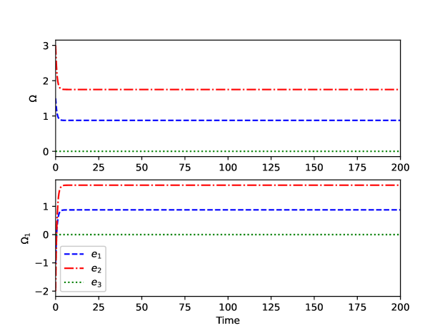
Figure 2: Trajectory converges to a permanent rotation about the principal axis corresponding to $A_{1}=A_{2}$.

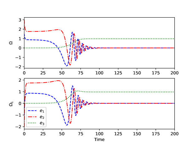
Figure 3: Trajectory converges to a permanent rotation about the principal axis corresponding to $A_{3}$.

Despite having “close” initial conditions, the trajectories from $z_{1}$ and $z_{2}$ converge to permanent rotations about different principal axes.

Figure 4 uses the same parameters with the initial condition $z=(1,0,0,0,1,0)^{T}$. One can verify that this initial data does not satisfy the conditions of Theorem 14(a); however, we can see that the solution still converges to the principal axis corresponding to the largest principal moment.

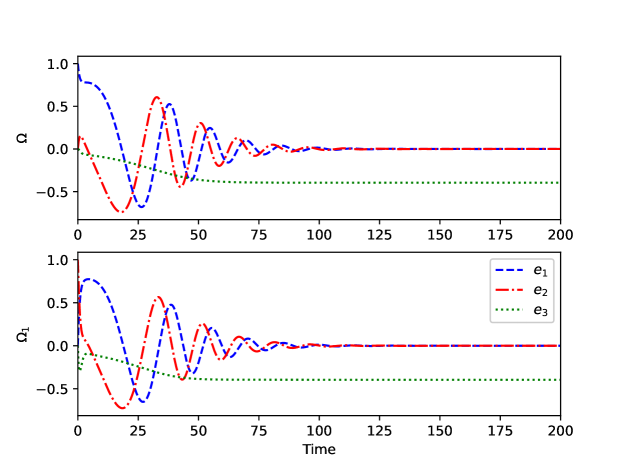
Figure 4: Initial data does not satisfy Theorem 14(a), yet still converges to $\bar{r}\neq 0$.

References

• \bibcommenthead
• (1) Boyce, W. E., DiPrima, R. C., Meade, D. B.: Elementary Differential Equations and Boundary Value Problems, 12th edn. Wiley, United States of America (2021)
• (2) Chernous’ko, F.L.: The Movement of a Rigid Body with Cavities Containing a Viscous Fluid. Mathematical methods in spacecraft dynamics, vol. v. 665. National Aeronautics and Space Administration, United States of America (1972)
• (3) Chernous’ko, F.L., Akulenko, L.D., Leshchenko, D.D.: Evolution of Motions of a Rigid Body About Its Center of Mass. Springer, Cham (2017)
• (4) Coddington, E. A., Levinson, N.: Theory of Ordinary Differential Equations. McGraw-Hill, India (1987)
• (5) Crandall, M. G., Rabinowitz, P. H.: Bifurcation, perturbation of simple eigenvalues, and linearized stability. Arch. Rat. Mech. Anal. 52(2), 161–180 (1973)
• (6) Disser, K., Galdi, G. P., Mazzone, G., Zunino, P.: Inertial motions of a rigid body with a cavity filled with a viscous liquid. Arch. Ration. Mech. Anal. 221(1), 487–526 (2016)
• (7) Farkas, B., Wegner, S.-A.: Variations on Barbălat’s Lemma. Am. Math. Mon. 123(8), 825–830 (2016)
• (8) Hale, J.K.: Ordinary Differential Equations. Dover Publications, United States of America (2009)
• (9) Mazzone, G.: On the dynamics of a rigid body with cavities completely filled by a viscous liquid. PhD thesis, University of Pittsburgh (2016)
• (10) Mazzone, G.: On the free rotations of rigid bodies with a liquid-filled gap. J. Math. Anal. Appl. 496(2), 124826–37 (2021)
• (11) Mazzone, G., Prüss, J., Simonett, G.: A maximal regularity approach to the study of motion of a rigid body with a fluid-filled cavity. J. Math. Fluid Mech. 21(3), 44 (2019)
• (12) Mazzone, G., Prüss, J., Simonett, G.: On the motion of a fluid-filled rigid body with Navier boundary conditions. SIAM J. Math. Anal. 51(3), 1582–1606 (2019)
• (13) Prüss, J.W., Wilke, M.: Gewöhnliche Differentialgleichungen und Dynamische Systeme, 2nd edn. Birkhäuser, Cham (in German) (2019)