Hubs and Hyperspheres: Reducing Hubness and Improving Transductive Few-shot Learning with Hyperspherical Embeddings

Abstract

Distance-based classification is frequently used in transductive few-shot learning (FSL). However, due to the high-dimensionality of image representations, FSL classifiers are prone to suffer from the hubness problem, where a few points (hubs) occur frequently in multiple nearest neighbour lists of other points. Hubness negatively impacts distance-based classification when hubs from one class appear often among the nearest neighbors of points from another class, degrading the classifier’s performance. To address the hubness problem in FSL, we first prove that hubness can be eliminated by distributing representations uniformly on the hypersphere. We then propose two new approaches to embed representations on the hypersphere, which we prove optimize a tradeoff between uniformity and local similarity preservation – reducing hubness while retaining class structure. Our experiments show that the proposed methods reduce hubness, and significantly improves transductive FSL accuracy for a wide range of classifiers.

1 Introduction

While supervised deep learning has made a significant impact in areas where large amounts of labeled data are available [1, 2], few-shot learning (FSL) has emerged as a promising alternative when labeled data is limited [3, 4, 5, 6, 7, 8, 9, 10, 11, 12, 13]. FSL aims to design classifiers that can discriminate between novel classes based on a few labeled instances, significantly reducing the cost of the labeling procedure.

In transductive FSL, one assumes access to the entire query set during evaluation. This allows transductive FSL classifiers to learn representations from a larger number of samples, resulting in better performing classifiers. However, many of these methods base their predictions on distances to prototypes for the novel classes [5, 6, 7, 8, 9, 11]. This makes these methods susceptible to the hubness problem [14, 15, 16, 17], where certain exemplar points (hubs) appear among the nearest neighbours of many other points. If a support sample is a hub, many query samples will be assigned to it regardless of their true label, resulting in low accuracy. If more training data is available, this effect can be reduced by increasing the number of labeled samples in the classification rule – but this is impossible in FSL.

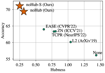
Figure 1: Few-shot accuracy increases when hubness decreases. The figure shows the 1-shot accuracy when classifying different embeddings with SimpleShot [4] on mini-ImageNet [18].

Several approaches have recently been proposed to embed samples in a space where the FSL classifier’s performance is improved [4, 19, 20, 21, 11, 22, 23]. However, only one of these directly addresses the hubness problem. Fei et al. [20] show that embedding representations on a hypersphere with zero mean reduces hubness. They advocate the use of Z-score normalization (ZN) along the feature axis of each representation, and show empirically that ZN can reduce hubness in FSL. However, ZN does not guarantee a data mean of zero, meaning that hubness can still occur after ZN.

In this paper we propose a principled approach to embed representations in FSL, which both reduces hubness and improves classification performance. First, we prove that hubness can be eliminated by embedding representations uniformly on the hypersphere. However, distributing representations uniformly on the hypersphere without any additional constraints will likely break the class structure which is present in the representation space – hurting the performance of the downstream classifier. Thus, in order to both reduce hubness and preserve the class structure in the representation space, we propose two new embedding methods for FSL. Our methods, Uniform Hyperspherical Structure-preserving Embeddings (noHub) and noHub with Support labels (noHub-S), leverage a decomposition of the Kullback-Leibler divergence between representation and embedding similarities, to optimize a tradeoff between Local Similarity Preservation (LSP) and uniformity on the hypersphere. The latter method, noHub-S, also leverages label information from the support samples to further increase the class separability in the embedding space.

Figure 1 illustrates the correspondence between hubness and accuracy in FSL. Our methods have both the least hubness and highest accuracy among several recent embedding techniques for FSL.

Our contributions are summarized as follows.

• We prove that the uniform distribution on the hypersphere has zero hubness and that embedding points uniformly on the hypersphere thus alleviates the hubness problem in distance-based classification for transductive FSL.

• We propose noHub and noHub-S to embed representations on the hypersphere, and prove that these methods optimize a tradeoff between LSP and uniformity. The resulting embeddings are therefore approximately uniform, while simultaneously preserving the class structure in the embedding space.

• Extensive experimental results demonstrate that noHub and noHub-S outperform current state-of-the-art embedding approaches, boosting the performance of a wide range of transductive FSL classifiers, for multiple datasets and feature extractors.

2 Related Work

The hubness problem.  The hubness problem refers to the emergence of hubs in collections of points in high-dimensional vector spaces [16]. Hubs are points that appear among the nearest neighbors of many other points, and are therefore likely to have a significant influence on e.g. nearest neighbor-based classification. Radovanovic et al. [16] showed that points closer to the expected data mean are more likely be among the nearest neighbors of other points, indicating that these points are more likely to be hubs. Hubness can also be seen as a result of large density gradients [24], as points in high-density areas are more likely to be hubs. The hubness problem is thus an intrinsic property of data distributions in high-dimensional vector spaces, and not an artifact occurring in particular datasets. It is therefore important to take the hubness into account when designing classification systems in high-dimensional vector spaces.

Hubness in FSL.  Many recent methods in FSL rely on distance-based classification in high-dimensional representation spaces [4, 5, 6, 25, 26, 27, 28], making them vulnerable to the hubness problem. Fei et al. [20] show that hyperspherical representations with zero mean reduce hubness. Motivated by this insight, they suggest that representations should have zero mean and unit standard deviation (ZN) along the feature dimension. This effectively projects samples onto the hyperplane orthogonal to the vector with all elements $=1$, and pushes them to the hypersphere with radius $\sqrt{d}$, where $d$ is the dimensionality of the representation space. Although ZN is empirically shown to reduce hubness, it does not guarantee that the data mean is zero. The normalized representations can therefore still suffer from hubness, potentially decreasing FSL performance.

Embeddings in FSL.  FSL classifiers often operate on embeddings of representations instead of the representations themselves, to improve the classifier’s ability to generalize to novel classes [4, 19, 11, 22]. Earlier works use the L2 normalization and Centered L2 normalization to embed representations on the hypersphere [4]. Among more recent embedding techniques, ReRep [19] performs a two-step fusing operation on both the support and query features with an attention mechanism. EASE [11] combines both support and query samples into a single sample set, and jointly learns a similarity and dissimilarity matrix, encouraging similar features to be embedded closer, and dissimilar features to be embedded far away. TCPR [22] computes the top-k neighbours of each test sample from the base data, computes the centroid, and removes the feature components in the direction of the centroid. Although these methods generally lead to a reduction in hubness and an increase in performance (see Figure 1), they are not explicitly designed to address the hubness problem resulting in suboptimal hubness reduction and performance. In contrast, our proposed noHub and noHub-S directly leverage our theoretic insights to target the root of the hubness problem.

Hyperspherical uniformity.  Benefits of uniform hyperspherical representations have previously been studied for contrastive self-supervised learning (SSL) [29]. Our work differs from [29] on several key points. First, we study a non-parametric embedding of support and query samples for FSL, which is a fundamentally different task from contrastive SSL. Second, the contrastive loss studied in [29] is a combination of different cross-entropies, making it different from our KL-loss. Finally, we introduce a tradeoff-parameter between uniformity and LSP, and connect our theoretical results to hubness and Laplacian Eigenmaps.

3 Hyperspherical Uniform Eliminates Hubness

We will now show that hubness can be eliminated completely by embedding representations uniformly on the hypersphere.

Definition 1 (Uniform PDF on the hypersphere.).

The uniform probability density function (PDF) on the unit hypersphere $\pazocal{\mathbb{S}}_{d}=\{\boldsymbol{x}\in{}^{d}\mid||\boldsymbol{x}||=1\}\subset{}^{d}$ is

$$u_{\mathbb{S}_{d}}(\boldsymbol{x})=A_{d}^{-1}\delta(||\boldsymbol{x}||-1)$$ (1)

where $A_{d}=\frac{2\pi^{d/2}}{\Gamma(d/2)}$ is the surface area of $\mathbb{S}_{d}$, and $\delta(\cdot)$ is the Dirac delta distribution.

We then have the following propositions for random vectors with this PDF.

Proposition 1.

Suppose $\boldsymbol{X}$ has PDF $u_{\mathbb{S}_{d}}(\boldsymbol{x})$. Then

$$\mathds{E}(\boldsymbol{X})=0$$ (2)

Proposition 2.

Let $\Pi_{\boldsymbol{p}}$ be the tangent plane of $\mathbb{S}_{d}$ at an arbitrary point $\boldsymbol{p}\in\mathbb{S}_{d}$. Then, for any direction $\boldsymbol{\theta}^{*}$ in $\Pi_{\boldsymbol{p}}$ the directional derivative of $u_{\mathbb{S}_{d}}$ along $\boldsymbol{\theta}^{*}$ is

$$\nabla_{\boldsymbol{\theta}^{*}}u_{\mathbb{S}_{d}}=0$$ (3)

These two propositions show that the hyperspherical uniform has (i) zero mean; and (ii) zero density gradient along all directions tangent to the hypersphere’s surface, at all points on the hypersphere. The hyperspherical uniform thus provably eliminates hubness, both in the sense of having a zero data mean, and having zero density gradient everywhere. We note that the latter property is un-attainable in Euclidean space, as it is impossible to define a uniform distribution over the whole space. It is therefore necessary to embed points on a non-Euclidean sub-manifold in order to eliminate hubness.

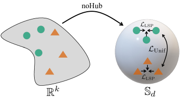
Figure 2: Illustration of the noHub embedding. Given representations $\in{}^{k}$, ${\pazocal{L}}_{\mathrm{LSP}}$ preserves local similarities. ${\pazocal{L}}_{\mathrm{Unif}}$ simultaneously encourages uniformity in the embedding space $\mathbb{S}_{d}$. This feature embedding framework helps reduce hubness while improving classification performance.

4 Method

In the preceding section, we proved that uniform embeddings on the hypersphere eliminate hubness. However, naïvely placing points uniformly on the hypersphere does not incorporate the inherent class structure in the data, leading to poor FSL performance. Thus, there exists a tradeoff between uniformity on the hypersphere and the preservation of local similarities. To address this tradeoff, we introduce two novel embedding approaches for FSL, namely noHub and noHub-S. noHub (Sec. 4.1) incorporates a novel loss function for embeddings on the hypersphere, while noHub-S (Sec. 4.2), guides noHub with additional label information, which should act as a supervisory signal for a class-aware embedding that leads to improved classification performance. Figure 2 provides an overview of the proposed noHub method. We also note that, since our approach generates embeddings, they are compatible with most transductive FSL classifier.

Few-shot Preliminaries.  Assume we have a large labeled base dataset $\pazocal{X}_{\text{Base}}=\{(\boldsymbol{x}_{i},y_{i})\mid y_{i}\in\pazocal{C}_{\text{Base}};\leavevmode\nobreak\ i=1,\ldots,n_{\text{Base}}\}$, where $\boldsymbol{x}_{i}$ and $y_{i}$ denotes the raw features and labels, respectively. Let $\pazocal{C}_{\text{Base}}$ denote the set of classes for the base dataset. In the few–shot scenario, we assume that we are given another labeled dataset $\pazocal{X}_{\text{Novel}}=\{(\boldsymbol{x}_{i},y_{i})\mid y_{i}\in\pazocal{C}_{\text{Novel}};\leavevmode\nobreak\ i=1,\ldots,n_{\text{Novel}}\}$ from novel, previously unseen classes $\pazocal{C}_{\text{Novel}}$, satisfying $\pazocal{C}_{\text{Base}}\cap\pazocal{C}_{\text{Novel}}=\emptyset$. In addition, we have a test set $\pazocal{T},\;\pazocal{T}\cap\pazocal{X}_{\text{Novel}}=\emptyset$, also from $\pazocal{C}_{\text{Novel}}$.

In a $K$–way $N_{S}$–shot FSL problem, we create randomly sampled tasks (or episodes), with data from $K$ randomly chosen novel classes. Each task consists of a support set $\pazocal{S}\subset\pazocal{X}_{\text{Novel}}$ and a query set $\pazocal{Q}\subset\pazocal{T}$. The support set contains $|\pazocal{S}|=N_{S}\cdot K$ random examples ($N_{S}$ random examples from each of the $K$ classes). The query set contains $|\pazocal{Q}|=N_{Q}\cdot K$ random examples, sampled from the same $K$ classes. The goal of FSL is then to predict the class of samples $\boldsymbol{x}\in\pazocal{Q}$ by exploiting the labeled support set $\pazocal{S}$, using a model trained on the base classes $\pazocal{C}_{\text{Base}}$. We assume a fixed feature extractor, trained on the base classes, which maps the raw input data to the representations $\boldsymbol{x}_{i}$.

4.1 noHub: Uniform Hyperspherical Structure-preserving Embeddings

We design an embedding method that encourages uniformity on the hypersphere, and simultaneously preserves local similarity structure. Given the support and query representations $\boldsymbol{x}_{1},\dots,\boldsymbol{x}_{n}\in{}^{k}$, $n=K(N_{S}+N_{Q})$ , we wish to find suitable embeddings $\boldsymbol{z}_{1},\dots,\boldsymbol{z}_{n}\in\mathbb{S}_{d}$, where local similarities are preserved. For both representations and embeddings, we quantify similarities using a softmax over pairwise cosine similarities

$$p_{ij}=\frac{p_{i|j}+p_{j|i}}{2},\quad p_{i|j}=\frac{\operatorname{exp}(\kappa_{i}\frac{\boldsymbol{x}_{i}^{\top}\boldsymbol{x}_{j}}{||\boldsymbol{x}_{i}||\cdot||\boldsymbol{x}_{j}||})}{\sum\limits_{l,m}\operatorname{exp}(\kappa_{i}\frac{\boldsymbol{x}_{l}^{\top}\boldsymbol{x}_{m}}{||\boldsymbol{x}_{l}||\cdot||\boldsymbol{x}_{m}||})}$$ (4)

and

$$q_{ij}=\frac{\operatorname{exp}(\kappa\boldsymbol{z}_{i}^{\top}\boldsymbol{z}_{j})}{\sum\limits_{l,m}\operatorname{exp}(\kappa\boldsymbol{z}_{l}^{\top}\boldsymbol{z}_{m})},$$ (5)

where $\kappa_{i}$ is chosen such that the effective number of neighbours of $\boldsymbol{x}_{i}$ equals a pre-defined perplexity. As in [30, 31], local similarity preservation can now be achieved by minimizing the Kullback-Leibler (KL) divergence between the $p_{ij}$ and the $q_{ij}$

$$KL(P||Q)=\sum\limits_{i,j}p_{ij}\log\frac{p_{ij}}{q_{ij}}.$$ (6)

However, instead of directly minimizing $KL(P||Q)$, we find that the minimization problem is equivalent to minimizing the sum of two loss functions

$$\operatorname*{arg\,min}\limits_{\boldsymbol{z}_{1},\dots,\boldsymbol{z}_{n}\in\pazocal{\mathbb{S}}_{d}}KL(P||Q)=\operatorname*{arg\,min}\limits_{\boldsymbol{z}_{1},\dots,\boldsymbol{z}_{n}\in\pazocal{\mathbb{S}}_{d}}{\pazocal{L}}_{\mathrm{LSP}}+{\pazocal{L}}_{\mathrm{Unif}}$$ (7)

where

$${\pazocal{L}}_{\mathrm{LSP}}=-\kappa\sum\limits_{i,j}p_{ij}\boldsymbol{z}_{i}^{\top}\boldsymbol{z}_{j},$$ (8)

$${\pazocal{L}}_{\mathrm{Unif}}=\log\sum\limits_{l,m}\operatorname{exp}(\kappa\boldsymbol{z}_{l}^{\top}\boldsymbol{z}_{m}).$$ (9)

Input: Features $\in{}^{k}$, $\{\boldsymbol{x}_{1},\dots,\boldsymbol{x}_{n}\}$; perplexity, $P$; number of iterations, $T$ ; learning rate, $\eta$.

Output: Embeddings $\in\mathbb{S}_{d}$, $\{\boldsymbol{z}_{1},\dots,\boldsymbol{z}_{n}\}$

Compute $p_{ij}$ from Eq (4)

Initialize solution $\boldsymbol{Z}^{0}=\{\boldsymbol{z}_{1},\dots,\boldsymbol{z}_{n}\}$ with PCA

for $i\leftarrow 1$ to $T$ do

       Compute $q_{ij}$ from Eq. (5)

       Compute gradients $\frac{\mathrm{d}{\pazocal{L}}_{\mathrm{noHub}}}{\mathrm{d}\boldsymbol{Z}}$, using loss from Eq. (10)

       Update $\boldsymbol{Z}^{t}$ using the ADAM optimizer with learning rate $\eta$ [32]

       Re-normalize elements of $\boldsymbol{Z}^{t}$ using $L_{2}$ normalization

      

end for

return $\boldsymbol{Z}^{T}$

Algorithm 1 noHub algorithm for embeddings on the hypersphere

In Sec. 5 we provide a thorough theoretical analysis of these losses, and how they relate to LSP and uniformity on the hypersphere. Essentially, ${\pazocal{L}}_{\mathrm{LSP}}$ is responsible for the local similarity preservation by ensuring that the embedding similarities ($\boldsymbol{z}_{i}^{\top}\boldsymbol{z}_{j}$) are high whenever the representation similarities ($p_{ij}$) are high. ${\pazocal{L}}_{\mathrm{Unif}}$ on the other hand, can be interpreted as a negative entropy on $\mathbb{S}_{d}$, and is thus minimized when the embeddings are uniformly distributed on $\mathbb{S}_{d}$. This is discussed in more detail in Sec. 5.

Based on the decomposition of the KL divergence, and the subsequent interpretation of the two terms, we formulate the loss in noHub as the following tradeoff between LSP and uniformity

$${\pazocal{L}}_{\mathrm{noHub}}=\alpha{\pazocal{L}}_{\mathrm{LSP}}+(1-\alpha){\pazocal{L}}_{\mathrm{Unif}}$$ (10)

where $\alpha$ is a weight parameter quantifying the tradeoff. ${\pazocal{L}}_{\mathrm{noHub}}$ can then be optimized directly with gradient descent. The entire procedure is outlined in Algorithm 1.

4.2 noHub-S: noHub with Support labels

In order to strengthen the class structure in the embedding space, we modify ${\pazocal{L}}_{\mathrm{LSP}}$ and ${\pazocal{L}}_{\mathrm{Unif}}$ by exploiting the additional information provided by the support labels. For ${\pazocal{L}}_{\mathrm{LSP}}$, we change the similarity function in $p_{ij}$ such that

$$p_{i|j}=\frac{\operatorname{exp}(\kappa_{i}s_{\boldsymbol{x}}(\boldsymbol{x}_{i},\boldsymbol{x}_{j}))}{\sum\limits_{l,m}\operatorname{exp}(\kappa_{i}s_{\boldsymbol{x}}(\boldsymbol{x}_{l},\boldsymbol{x}_{m}))}$$ (11)

where

$$s_{\boldsymbol{x}}(\boldsymbol{x}_{i},\boldsymbol{x}_{j})=\begin{cases}1&\text{if $\boldsymbol{x}_{i},\boldsymbol{x}_{j}\in\pazocal{S}$, and $y_{i}=y_{j}$}\\ -1&\text{if $\boldsymbol{x}_{i},\boldsymbol{x}_{j}\in\pazocal{S}$, and $y_{i}\neq y_{j}$}\\ $$\boldsymbol{x}_{i}^{\top}\boldsymbol{x}_{j}$$&\text{otherwise}\end{cases}.$$ (12)

With this, we encourage embeddings for support samples in the same class to be maximally similar, and support samples in different classes to be maximally dissimilar. Similarly, for ${\pazocal{L}}_{\mathrm{Unif}}$

$${\pazocal{L}}_{\mathrm{Unif}}=\log\sum\limits_{l,m}\operatorname{exp}(\kappa s_{\boldsymbol{z}}(\boldsymbol{z}_{i},\boldsymbol{z}_{j}))$$ (13)

where

$$s_{\boldsymbol{z}}(\boldsymbol{z}_{i},\boldsymbol{z}_{j})=\begin{cases}-\infty,&\text{if $\boldsymbol{z}_{i},\boldsymbol{z}_{j}\in\pazocal{S}$, and $y_{i}=y_{j}$}\\ \varepsilon\leavevmode\nobreak\ \boldsymbol{z}_{i}^{\top}\boldsymbol{z}_{j},&\text{if $\boldsymbol{z}_{i},\boldsymbol{z}_{j}\in\pazocal{S}$, and $y_{i}\neq y_{j}$}\\ \boldsymbol{z}_{i}^{\top},\boldsymbol{z}_{j}&\text{otherwise}\end{cases}$$ (14)

where $\varepsilon$ is a hyperparameter. This puts more emphasis on between-class uniformity by weighting the similarity higher for embeddings belonging to different classes ($\varepsilon>1$), and ignoring the similarity between embeddings belonging to the same class. The final loss function is the same as Eq. (10), but with the additional label-informed similarities in Eqs. (11)–(14).

5 Theoretical Results

In this section we provide a theoretical analysis of ${\pazocal{L}}_{\mathrm{LSP}}$ and ${\pazocal{L}}_{\mathrm{Unif}}$. Based on our analysis, we interpret these losses with regards to the Laplacian Eigenmaps algorithm and Rényi entropy, respectively.

Proposition 3.

Let $W_{ij}=\frac{1}{2}\kappa p_{ij}$, where $\sum\limits_{i,j}p_{ij}=1$, and let $\boldsymbol{z}_{1},\dots,\boldsymbol{z}_{n}\in\pazocal{\mathbb{S}}_{d}$. Then we have

$${\pazocal{L}}_{\mathrm{LSP}}=\sum_{i,j}\|\boldsymbol{z}_{i}-\boldsymbol{z}_{j}\|^{2}W_{ij}-\kappa.$$ (15)

Proposition 4 (Minimizing ${\pazocal{L}}_{\mathrm{Unif}}$ maximizes entropy).

Let $H_{2}(\cdot)$ be the 2-order Rényi entropy, estimated with a kernel density estimator using a Gaussian kernel. Then

$$\operatorname*{arg\,min}\limits_{\boldsymbol{z}_{1},\dots,\boldsymbol{z}_{n}\in\pazocal{\mathbb{S}}_{d}}{\pazocal{L}}_{\mathrm{Unif}}=\operatorname*{arg\,max}\limits_{\boldsymbol{z}_{1},\dots,\boldsymbol{z}_{n}\in\pazocal{\mathbb{S}}_{d}}H_{2}(\boldsymbol{z}_{1},\dots,\boldsymbol{z}_{n}).$$ (16)

Definition 2 (Normalized counting measure).

The normalized counting measure associated with a set $B$ on $A$ is

$$\nu_{B}(A)=\frac{|B\cap A|}{|B|}$$ (17)

Definition 3 (Normalized surface area measure on $\mathbb{S}_{d}$).

The normalized surface area measure on the hyperspehere $\mathbb{S}_{d}\subset{}^{d}$, of a subset $S^{\prime}\subset\mathbb{S}_{d}$ is

$$\sigma_{d}(S^{\prime})=\frac{\int_{S^{\prime}}\mathrm{d}S}{\int_{\mathbb{S}_{d}}\mathrm{d}S}=A_{d}^{-1}\int_{S^{\prime}}\mathrm{d}S$$ (18)

where $A_{d}$ is defined as in Eq. (1), and $\int\mathrm{d}S$ denotes the surface integral on $\mathbb{S}_{d}$.

Definition 4 (Weak^∗ convergence of measures [29]).

A sequence of Borel measures $\{\mu_{n}\}_{n=1}^{\infty}$ in ^d converges weak^∗ to a Borel measure $\mu$, if for all continuous functions $f:{}^{d}\to\real$,

$$\lim\limits_{n\to\infty}\int f(x)\mathrm{d}\mu_{n}(x)=\int f(x)\mathrm{d}\mu(x)$$ (19)

Proposition 5 (Minimizer of ${\pazocal{L}}_{\mathrm{Unif}}$).

For each $n>0$, the $n$ point minimizer of ${\pazocal{L}}_{\mathrm{Unif}}$ is

$$\boldsymbol{z}_{1}^{\star},\dots,\boldsymbol{z}_{n}^{\star}=\operatorname*{arg\,min}\limits_{\boldsymbol{z}_{1},\dots,\boldsymbol{z}_{n}\in\pazocal{\mathbb{S}}_{d}}{\pazocal{L}}_{\mathrm{Unif}}.$$ (20)

Then $\nu_{\{\boldsymbol{z}_{1}^{\star},\dots,\boldsymbol{z}_{n}^{\star}\}}$ converge weak^∗ to $\sigma_{d}$ as $n\to\infty$.

Interpretation of Proposition 3–5.  Proposition 3 states an alternative formulation of ${\pazocal{L}}_{\mathrm{LSP}}$, under the hyperspherical assumption. We recognize this formulation as the loss function in Laplacian Eigenmaps [33], which is known to produce local similarity-preserving embeddings from graph data. When unconstrained, this loss has a trivial solution where the embeddings for all representations are equal. This is avoided in our case since ${\pazocal{L}}_{\mathrm{noHub}}$ (Eq. (10)) can be interpreted as the Lagrangian of minimizing ${\pazocal{L}}_{\mathrm{LSP}}$ subject to a specified level of entropy, by Proposition 4.

Finally, Proposition 5 states that the normalized counting measure associated with the set of points that minimize ${\pazocal{L}}_{\mathrm{Unif}}$, converges to the normalized surface area measure on the sphere. Since $u_{\mathbb{S}_{d}}$ is the density function associated with this measure, the points that minimize ${\pazocal{L}}_{\mathrm{Unif}}$ will tend to be uniform on the sphere. Consequently, minimizing ${\pazocal{L}}_{\mathrm{LSP}}$ also minimizes hubness, by Propositions 1 and 2.

6 Experiments

6.1 Setup

		mini		tiered		CUB
Embedding	Feature Extractor	1-shot ​$\uparrow$	5-shot ​$\uparrow$	1-shot ​$\uparrow$	5-shot ​$\uparrow$	1-shot ​$\uparrow$	5-shot ​$\uparrow$
None	ResNet-18	20.0 (0.0)∗	20.0 (0.0)∗	20.0 (0.0)∗	20.0 (0.0)∗	20.0 (0.0)∗	20.0 (0.0)∗
L2 (ArXiv’19 [4])	ResNet-18	73.77 (0.24)	83.14 (0.14)	80.46 (0.26)	87.04 (0.16)	83.1 (0.23)	89.48 (0.12)
CL2 (ArXiv’19 [4])	ResNet-18	75.56 (0.26)	84.04 (0.15)	82.1 (0.26)	87.9 (0.16)	84.35 (0.24)	90.14 (0.12)
ZN (ICCV’21 [20])	ResNet-18	20.0 (0.0)∗	20.0 (0.0)∗	20.0 (0.0)∗	20.0 (0.0)∗	20.0 (0.0)∗	20.0 (0.0)∗
ReRep (ICML’21 [19])	ResNet-18	20.0 (0.0)∗	20.0 (0.0)∗	20.0 (0.0)∗	20.0 (0.0)∗	20.0 (0.0)∗	20.0 (0.0)∗
EASE (CVPR’22 [11])	ResNet-18	76.05 (0.27)	84.61 (0.15)	82.57 (0.27)	88.33 (0.16)	85.24 (0.24)	90.42 (0.12)
TCPR (NeurIPS’22 [22])	ResNet-18	75.99 (0.26)	84.39 (0.15)	82.65 (0.26)	88.26 (0.16)	85.34 (0.23)	90.5 (0.11)
noHub (Ours)	ResNet-18	76.65 (0.28)	84.05 (0.16)	82.94 (0.27)	87.87 (0.17)	85.88 (0.24)	90.34 (0.12)
noHub-S (Ours)	ResNet-18	76.68 (0.28)	84.67 (0.15)	83.09 (0.27)	88.43 (0.16)	85.81 (0.24)	90.52 (0.12)
None	WideRes28-10	45.69 (0.31)	58.82 (0.31)	75.29 (0.28)	82.56 (0.22)	61.36 (0.55)	82.22 (0.37)
L2 (ArXiv’19 [4])	WideRes28-10	80.2 (0.23)	87.11 (0.13)	80.89 (0.26)	87.34 (0.15)	91.98 (0.18)	94.15 (0.1)
CL2 (ArXiv’19 [4])	WideRes28-10	75.23 (0.27)	83.99 (0.16)	79.59 (0.27)	86.71 (0.16)	92.17 (0.18)	94.48 (0.09)
ZN (ICCV’21 [20])	WideRes28-10	20.0 (0.0)∗	20.0 (0.0)∗	20.0 (0.0)∗	20.0 (0.0)∗	20.0 (0.0)∗	20.0 (0.0)∗
ReRep (ICML’21 [19])	WideRes28-10	36.69 (0.28)	36.41 (0.3)	67.41 (0.29)	76.49 (0.24)	57.62 (0.56)	60.36 (0.6)
EASE (CVPR’22 [11])	WideRes28-10	81.19 (0.25)	87.82 (0.13)	82.04 (0.26)	88.06 (0.16)	91.99 (0.19)	94.36 (0.09)
TCPR (NeurIPS’22 [22])	WideRes28-10	81.27 (0.24)	87.8 (0.13)	81.89 (0.26)	87.95 (0.16)	91.91 (0.18)	94.25 (0.1)
noHub (Ours)	WideRes28-10	81.97 (0.25)	87.78 (0.14)	82.8 (0.27)	87.99 (0.17)	92.53 (0.18)	94.56 (0.09)
noHub-S (Ours)	WideRes28-10	82.0 (0.26)	88.03 (0.13)	82.85 (0.27)	88.31 (0.16)	92.63 (0.18)	94.69 (0.09)

Table 1: Accuracies (Confidence interval) with the SIAMESE [11] classifier for different embedding approaches. Best and second best performance are denoted in bold and underlined, respectively. ^∗The SIAMESE classifier is sensitive to the norm of the embedding, thus leading to detrimental performance for some of the embedding approaches.

Implementation details.  Our implementation is in PyTorch [34]. We optimize noHub and noHub-S for $T=150$ iterations, using the Adam optimizer [32] with learning rate $\eta=0.1$. The other hyperparameters were chosen based on validation performance on the respective datasets. We analyze the effect of $\alpha$ in Sec. 6.2. Analyses of the $\kappa$ and $\varepsilon$ hyperparameters are provided in the supplementary.

Initialization.  Since noHub and noHub-S reduce the embedding dimensionality ($d=400$), we initialize embeddings with Principal Component Analysis (PCA) [35], instead of a naïve, random initialization. The PCA initialization is computationally efficient, and approximately preserves global structure. It also resulted in faster convergence and better performance, compared to random initialization.

Base feature extractors.  We use the standard networks ResNet-18 [1] and Wide-Res28-10 [36] as the base feature extractors with pretrained weights from [7] and [37], respectively.

Datasets.  Following common practice, we evaluate FSL performance on the mini-ImageNet (mini) [18], tiered-ImageNet (tiered) [38], and CUB-200 (CUB) [39] datasets.

Classifiers.  We evaluate the baseline embeddings and our proposed methods using both established and recent FSL classifiers: SimpleShot [4], LaplacianShot [5], $\mathit{\alpha}-$TIM [7], Oblique Manifold (OM) [8], iLPC [9], and SIAMESE [11].

Baseline Embeddings.  We compare our proposed method with a wide range of techniques for embedding the base features: None (No embedding of base features), L2 [4], Centered L2 [4], ZN [20], ReRep [19], EASE [11], and TCPR [22].

Evaluation protocol.  We follow the standard evaluation protocol in FSL and calculate the accuracy for 1-shot and 5-shot classification with 15 images per class in the query set. We evaluate on $10000$ episodes, as is standard practice in FSL. Additionally, we evaluate the hubness of the representations after embedding using two common hubness metrics, namely the skewness (Sk) of the k-occurrence distribution [16] and the hub occurrence (HO) [40], which measures the percentage of hubs in the nearest neighbour lists of all points.

6.2 Results

Comparison to the state-of-the-art.  To illustrate the effectiveness of noHub and noHub-S as an embedding approach for FSL, we consider the current state-of-the-art FSL method, which leverages the EASE embedding and obtains query predictions with SIAMESE [11]. We replace EASE with our proposed embedding approaches noHub and noHub-S, as well as other baseline embeddings, and evaluate performance on all datasets in the 1 and 5-shot setting. As shown in Table 1, noHub and noHub-S outperform all baseline approaches in both settings across all datasets, illustrating noHub’s and noHub-S’ ability to provide useful FSL embeddings, and updating the state-of-the-art in transductive FSL.

Aggregated FSL performance.  To further evaluate the general applicability of noHub and noHub-S as embedding approaches, we perform extensive experiments for all classifiers and all baseline embeddings on all datasets. Tables 2(a) and 2(b) provide the results averaged over classifiers. To clearly present the results, we aggregate the accuracy and a ranking score for each embedding method across all classifiers. The ranking score is calculated by performing a paired Student’s t-test between all pairwise embedding methods for each classifier. We then average the ranking scores across all classifiers. A high ranking score then indicates that a method often significantly outperforms the competing embedding methods. We set the significance level to 5%. noHub and noHub-S consistently outperform previous embedding approaches – sometimes by a large margin. Overall, we further observe that noHub-S outperforms noHub in most settings and is particular beneficial in the 1-shot setting, which is more challenging, given that fewer samples are likely to generate noisy embeddings.

		mini		tiered		CUB
	Embedding	Acc ​$\uparrow$	Score ​$\uparrow$	Acc ​$\uparrow$	Score ​$\uparrow$	Acc ​$\uparrow$	Score ​$\uparrow$
ResNet18	None	55.74	0.17	62.61	0.0	63.78	0.17
	L2 (ArXiv’19 [4])	68.22	2.33	75.94	2.17	78.09	2.33
	CL2 (ArXiv’19 [4])	69.56	2.83	76.97	3.0	78.26	2.83
	ZN (ICCV’21 [20])	60.0	2.33	66.21	2.5	67.43	2.67
	ReRep (ICML’21 [19])	60.76	4.0	67.07	3.67	69.6	4.17
	EASE (CVPR’22 [11])	69.63	3.67	77.05	4.0	78.84	3.67
	TCPR (NeurIPS’22 [22])	69.97	4.0	77.18	3.33	78.83	4.0
	noHub (Ours)	72.58	6.83	79.77	6.83	81.91	6.83
	noHub-S (Ours)	73.64	7.67	80.6	7.67	83.1	7.67
WideRes28-10	None	63.59	1.0	71.29	0.83	79.23	1.17
	L2 (ArXiv’19 [4])	74.3	3.0	76.19	2.67	88.61	3.5
	CL2 (ArXiv’19 [4])	71.32	1.33	75.17	2.0	88.52	3.33
	ZN (ICCV’21 [20])	64.27	2.5	65.64	2.5	76.0	1.5
	ReRep (ICML’21 [19])	65.51	3.0	71.83	3.17	83.1	3.5
	EASE (CVPR’22 [11])	74.95	4.33	76.59	3.67	88.51	3.5
	TCPR (NeurIPS’22 [22])	75.64	4.83	76.51	4.0	88.22	2.5
	noHub (Ours)	78.22	7.0	79.76	7.0	90.25	5.67
	noHub-S (Ours)	79.24	7.67	80.46	7.67	90.82	7.67

(a) 1-shot

		mini		tiered		CUB
		Acc ​$\uparrow$	Score ​$\uparrow$	Acc ​$\uparrow$	Score ​$\uparrow$	Acc ​$\uparrow$	Score ​$\uparrow$
ResNet18	None	69.83	0.83	74.38	0.67	76.01	1.17
	L2 (ArXiv’19 [4])	81.58	2.33	86.05	1.83	88.43	2.83
	CL2 (ArXiv’19 [4])	81.95	2.67	86.43	3.0	88.49	2.5
	ZN (ICCV’21 [20])	71.49	4.0	75.32	3.83	76.92	3.5
	ReRep (ICML’21 [19])	70.25	2.5	74.52	1.83	76.43	2.5
	EASE (CVPR’22 [11])	81.84	3.5	86.4	3.17	88.57	3.5
	TCPR (NeurIPS’22 [22])	82.1	4.0	86.54	3.83	88.79	4.33
	noHub (Ours)	82.58	5.5	86.9	4.5	89.13	6.0
	noHub-S (Ours)	82.61	6.5	87.13	6.67	88.93	5.33
WideRes28-10	None	78.77	1.5	84.1	1.67	89.49	1.67
	L2 (ArXiv’19 [4])	85.65	4.0	86.29	3.83	93.47	3.67
	CL2 (ArXiv’19 [4])	83.14	1.33	85.47	1.5	93.49	4.0
	ZN (ICCV’21 [20])	74.61	4.33	75.34	5.0	81.02	3.17
	ReRep (ICML’21 [19])	73.86	1.83	81.51	1.67	87.2	2.0
	EASE (CVPR’22 [11])	85.51	3.5	86.29	3.33	93.34	3.5
	TCPR (NeurIPS’22 [22])	86.03	6.0	86.37	4.0	93.3	3.0
	noHub (Ours)	86.44	5.67	87.07	5.5	93.65	4.17
	noHub-S (Ours)	85.95	5.5	87.05	5.83	93.76	5.0

(b) 5-shot

Table 2: Aggregated FSL performance for all embedding approaches on the mini-ImageNet, tiered-ImageNet, and CUB-200 datasets. Results are averaged over FSL classifiers. Best and second best performance are denoted in bold and underlined, respectively.

Hubness metrics.  To further validate noHub’s and noHub-S’ ability to reduce hubness, we follow the same procedure of aggregating results for the hubness metrics and average over classifiers. Compared to the current state-of-the-art embedding approaches, Table 3 illustrates that noHub and noHub-S consistently result in embeddings with lower hubness.

		mini		tiered		CUB
		Sk ​$\downarrow$	HO ​$\downarrow$	Sk ​$\downarrow$	HO ​$\downarrow$	Sk ​$\downarrow$	HO ​$\downarrow$
ResNet18	None	1.349	0.407	1.211	0.408	0.887	0.341
	L2 (ArXiv’19 [4])	0.937	0.301	0.812	0.265	0.691	0.236
	CL2 (ArXiv’19 [4])	0.667	0.233	0.679	0.249	0.549	0.201
	ZN (ICCV’21 [20])	0.68	0.231	0.698	0.264	0.564	0.216
	ReRep (ICML’21 [19])	3.655	0.548	3.604	0.549	3.565	0.513
	EASE (CVPR’22 [11])	0.521	0.16	0.479	0.158	0.466	0.153
	TCPR (NeurIPS’22 [22])	0.651	0.228	0.65	0.25	0.532	0.204
	noHub (Ours)	0.315	0.095	0.303	0.102	0.32	0.112
	noHub-S (Ours)	0.276	0.13	0.283	0.127	0.296	0.162
WideRes28-10	None	1.6	0.459	1.81	0.494	1.073	0.369
	L2 (ArXiv’19 [4])	0.781	0.296	0.737	0.275	0.475	0.228
	CL2 (ArXiv’19 [4])	0.981	0.288	0.817	0.307	0.52	0.267
	ZN (ICCV’21 [20])	0.73	0.287	0.769	0.302	0.517	0.263
	ReRep (ICML’21 [19])	3.56	0.704	3.55	0.777	3.026	0.47
	EASE (CVPR’22 [11])	0.47	0.177	0.477	0.175	0.437	0.213
	TCPR (NeurIPS’22 [22])	0.589	0.236	0.685	0.264	0.477	0.231
	noHub (Ours)	0.29	0.111	0.301	0.111	0.188	0.108
	noHub-S (Ours)	0.258	0.148	0.274	0.135	0.162	0.13

(a) 1-shot

		mini		tiered		CUB
		Sk ​$\downarrow$	HO ​$\downarrow$	Sk ​$\downarrow$	HO ​$\downarrow$	Sk ​$\downarrow$	HO ​$\downarrow$
ResNet18	None	1.436	0.422	1.339	0.432	0.987	0.364
	L2 (ArXiv’19 [4])	1.04	0.318	0.914	0.287	0.812	0.263
	CL2 (ArXiv’19 [4])	0.786	0.264	0.821	0.28	0.698	0.236
	ZN (ICCV’21 [20])	0.806	0.264	0.839	0.296	0.716	0.25
	ReRep (ICML’21 [19])	1.631	0.863	1.721	0.872	1.432	0.869
	EASE (CVPR’22 [11])	0.624	0.186	0.598	0.183	0.607	0.186
	TCPR (NeurIPS’22 [22])	0.78	0.259	0.796	0.283	0.687	0.235
	noHub (Ours)	0.286	0.096	0.289	0.104	0.329	0.12
	noHub-S (Ours)	0.25	0.074	0.213	0.078	0.433	0.097
WideRes28-10	None	1.709	0.473	1.937	0.51	1.16	0.395
	L2 (ArXiv’19 [4])	0.887	0.322	0.86	0.305	0.632	0.266
	CL2 (ArXiv’19 [4])	1.12	0.318	0.956	0.337	0.701	0.31
	ZN (ICCV’21 [20])	0.858	0.32	0.912	0.335	0.699	0.305
	ReRep (ICML’21 [19])	1.597	0.819	1.617	0.846	1.299	0.549
	EASE (CVPR’22 [11])	0.579	0.199	0.585	0.193	0.572	0.241
	TCPR (NeurIPS’22 [22])	0.717	0.27	0.815	0.294	0.634	0.264
	noHub (Ours)	0.294	0.115	0.298	0.115	0.195	0.1
	noHub-S (Ours)	0.494	0.103	0.407	0.12	0.421	0.127

(b) 5-shot

Table 3: Aggregated hubness metrics for all embedding approaches on the Mini-ImageNet, Tiered-ImageNet and CUB-200 dataset. Results are averaged over FSL classifiers. Best and second best performance are denoted in bold and underlined, respectively.

Visualization of similarity matrices.  As discussed in Sec. 4, completely eliminating hubness by distributing points uniformly on the hypersphere is not sufficient to obtain good FSL performance. Instead, representations need to also capture the inherent class structure of the data. To further evaluate the embedding approaches, we therefore compute the pairwise inner products for the embeddings of a random 5-shot episode on tiered-ImageNet with ResNet-18 features in Figure 3. It can be observed that the block structure is considerably more distinct for noHub and noHub-S, with noHub-S slightly improving upon noHub. These results indicate that (i) samples are more uniform, indicating the reduced hubness; and (ii) classes are better separated, due to the local similarity preservation.

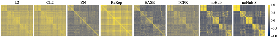
Figure 3: Inner product matrices between features for a random episode for all embedding approaches.

Tradeoff between uniformity and similarity preservation.  We analyze the effect of $\alpha$ on the tradeoff between LSP and Uniformity in the loss function in Eq. (10), on tiered-ImageNet with ResNet-18 features in the 5-shot setting and with the SIAMESE [11] classifier. The results are visualized in Figure 4. We notice a sharp increase in performance when we have a high emphasis on uniformity. This demonstrates the impact of hubness on accuracy in FSL performance. As we keep increasing the emphasis on LSP, however, after a certain point we notice a sharp drop off in performance. This is due to the fact that the classifier does not take into account the uniformity constraint on the features, resulting in a large number of misclassifications. In general, we observe that noHub-S is slightly more robust compared to noHub.

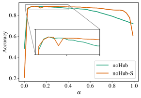
Figure 4: Accuracies for different values of the weighting parameter, $\alpha$, which quantifies the tradeoff between ${\pazocal{L}}_{\mathrm{LSP}}$ and ${\pazocal{L}}_{\mathrm{Unif}}$.

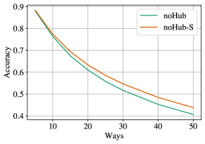
Figure 5: Accuracies for an increasing number of classes (ways) for noHub and noHub-S.

Increasing number of classes.  We analyze the behavior of noHub and noHub-S for an increasing number of classes (ways) on the tiered-ImageNet dataset with SIAMESE [11] as classifier. While classification accuracy generally decreases with an increasing number of classes, which is expected, we observe from Figure 5 that noHub-S has a slower decay and is able to leverage the label guidance to obtain better performance for a larger number of classes.

Effect of label information in ${\pazocal{L}}_{\mathrm{LSP}}$ and ${\pazocal{L}}_{\mathrm{Unif}}$.  To validate the effectiveness of using label guidance in noHub-S, we study the result of including label information in ${\pazocal{L}}_{\mathrm{LSP}}$ and ${\pazocal{L}}_{\mathrm{Unif}}$ (Eqs. (11)–(14)). We note that the default setting of noHub is that none of the two losses include label information. Ablation experiments are performed on tiered-ImageNet with the ResNet-18 feature extractor and the SimpleShot and SIAMESE classifier [11]. In Table LABEL:tab:ablation, we generally see improvements of noHub-S when both the loss terms are label-informed, indicating the usefulness of label guidance.

We further observe that incorporating label information in ${\pazocal{L}}_{\mathrm{Unif}}$ tends to have a larger contribution than doing the same for ${\pazocal{L}}_{\mathrm{LSP}}$. This aligns with our observations in Figure 4, where a small $\alpha$ yielded the best performance.

7 Conclusion

In this paper we have addressed the hubness problem in FSL. We have shown that hubness is eliminated by embedding representations uniformly on the hypersphere. The hyperspherical uniform distribution has zero mean and zero density gradient at all points along all directions tangent to the hypersphere – both of which are identified as causes of hubness in previous work [16, 24]. Based on our theoretical findings about hubness and hyperspheres, we proposed two new methods to embed representations on the hypersphere for FSL. The proposed noHub and noHub-S leverage a decomposition of the KL divergence between similarity distributions, and optimize a tradeoff between LSP and uniformity on the hypersphere – thus reducing hubness while maintaining the class structure in the representation space. We have provided theoretical analyses and interpretations of the LSP and uniformity losses, proving that they optimize LSP and uniformity, respectively. We comprehensively evaluate the proposed methods on several datasets, features extractors, and classifiers, and compare to a number of recent state-of-the-art baselines. Our results illustrate the effectiveness of our proposed methods and show that we achieve state-of-the-art performance in transductive FSL.

Appendix A Introduction

Here we provide proofs for our theoretical results on the hyperspherical uniform and hubness; the decomposition of the KL divergence; and the minima of our methods’ loss functions. We also give additional details on the implementation and hyperparameters for noHub and noHub-S– and include the complete tables of 1-shot and 5-shot results for all classifiers, datasets and feature extractors. Finally, we briefly reflect on potential negative societal impacts of our work.

Appendix B Hyperspherical Uniform Eliminates Hubness

Proof of Proposition 1

Lemma 1 (Trisection of hypersphere).

The trisection of the hypersphere along coordinate $i$ is given by the three-tuple of disjoint sets $(\mathbb{S}_{d}^{i,+},\mathbb{S}_{d}^{i,-},\mathbb{S}_{d}^{i,0})$ where

$$\mathbb{S}_{d}^{i,+}=\{\boldsymbol{x}=[x^{1},\dots,x^{d}]^{\top}\in\mathbb{S}_{d}\mid x^{i}>0\}$$ (21)

$$\mathbb{S}_{d}^{i,-}=\{\boldsymbol{x}=[x^{1},\dots,x^{d}]^{\top}\in\mathbb{S}_{d}\mid x^{i}<0\}$$ (22)

$$\mathbb{S}_{d}^{i,0}=\{\boldsymbol{x}=[x^{1},\dots,x^{d}]^{\top}\in\mathbb{S}_{d}\mid x^{i}=0\}$$ (23)

and

$$\mathbb{S}_{d}^{i,+}\cup\mathbb{S}_{d}^{i,-}\cup\mathbb{S}_{d}^{i,0}=\mathbb{S}_{d}$$ (24)

Then we have

$$\mathbb{S}_{d}^{i,+}=-\mathbb{S}_{d}^{i,-}=\{-\boldsymbol{x}\mid\boldsymbol{x}\in\mathbb{S}_{d}^{i,-}\}$$ (25)

Proof.

Let $\boldsymbol{x}\in\mathbb{S}_{d}^{i,+}$, then

$$||(-x)||=||x||=1,$$ (26)

and

$$-(x^{i})<0.$$ (27)

Hence $\boldsymbol{x}\in-\mathbb{S}_{d}^{i,-}$, and $\mathbb{S}_{d}^{i,+}\subseteq-\mathbb{S}_{d}^{i,-}$.

Similarly, let $-\boldsymbol{x}\in-\mathbb{S}_{d}^{i,-}$, then

$$||-(-x)||=||x||=1,$$ (28)

and

$$-(-x^{i})=x^{i}>0.$$ (29)

Hence $\boldsymbol{x}\in\mathbb{S}_{d}^{i,+}$, and $-\mathbb{S}_{d}^{i,-}\subseteq\mathbb{S}_{d}^{i,+}$.

It then follows that $\mathbb{S}_{d}^{i,+}=-\mathbb{S}_{d}^{i,-}$. ∎

Proof (Proposition 1).

The expectation $\mathds{E}(\boldsymbol{X})$ is given by

$$\mathds{E}(\boldsymbol{X})=\int_{{}^{d}}\boldsymbol{x}u_{\mathbb{S}_{d}}(\boldsymbol{x})\mathrm{d}\boldsymbol{x}$$ (30)

Since $u_{\mathbb{S}_{d}}$ is non-zero only on the hypersphere $\mathbb{S}_{d}$, the integral can be rewritten as a surface integral over $\mathbb{S}_{d}$

$$\mathds{E}(\boldsymbol{X})=\int_{\mathbb{S}_{d}}\boldsymbol{x}A_{d}^{-1}\mathrm{d}S.$$ (31)

Decomposing the integral over the trisection of $\mathbb{S}_{d}$ along coordinate $i$ gives

$$\int_{\mathbb{S}_{d}}\boldsymbol{x}A_{d}^{-1}\mathrm{d}S=$$ (32)

$$A_{d}^{-1}\left(\int_{\mathbb{S}_{d}^{i,+}}\boldsymbol{x}\mathrm{d}S+\int_{\mathbb{S}_{d}^{i,-}}\boldsymbol{x}\mathrm{d}S+\int_{\mathbb{S}_{d}^{i,0}}\boldsymbol{x}\mathrm{d}S\right).$$ (33)

By Lemma 1 we have

$$\mathbb{S}_{d}^{i,+}=-\mathbb{S}_{d}^{i,-}\Rightarrow\int_{\mathbb{S}_{d}^{i,+}}\boldsymbol{x}\mathrm{d}S=-\int_{\mathbb{S}_{d}^{i,-}}\boldsymbol{x}\mathrm{d}S.$$ (34)

Furthermore, since the set $\mathbb{S}_{d}^{i,0}$ has zero width along coordinate $i$, $\int_{\mathbb{S}_{d}^{i,0}}\boldsymbol{x}\mathrm{d}S=0$. Hence

$$\mathds{E}(\boldsymbol{X})=$$ (35)

$$A_{d}^{-1}\left(\int_{\mathbb{S}_{d}^{i,+}}\boldsymbol{x}\mathrm{d}S-\int_{\mathbb{S}_{d}^{i,+}}\boldsymbol{x}\mathrm{d}S+\int_{\mathbb{S}_{d}^{i,0}}\boldsymbol{x}\mathrm{d}S\right)=0$$ (36)

∎

Proof of Proposition 2

Proof.

$u_{\mathbb{S}_{d}}(\boldsymbol{x})$ can be written in polar coordinates as

$$u_{\mathbb{S}_{d}}(\boldsymbol{x}(r,\boldsymbol{\theta}))=u_{\mathbb{S}_{d}}^{\text{Polar}}(r,\boldsymbol{\theta})=A_{d}^{-1}\delta(r-1)$$ (37)

The gradient of $u_{\mathbb{S}_{d}}^{\text{Polar}}(r,\boldsymbol{\theta})$ is then

$$\nabla_{(r,\boldsymbol{\theta})}u_{\mathbb{S}_{d}}^{\text{Polar}}(r,\boldsymbol{\theta})=\begin{bmatrix}\frac{\partial}{\partial r}u_{\mathbb{S}_{d}}^{\text{Polar}}(r,\boldsymbol{\theta})\\[5.69046pt] 0\\ \vdots\\ 0\end{bmatrix}$$ (38)

For an arbitrary point $\boldsymbol{p}\in\mathbb{S}_{d}$, an arbitrary unit vector (direction), $\boldsymbol{\theta}^{*}$, in the tangent plane $\Pi_{\boldsymbol{p}}$ is given by

$$\boldsymbol{\theta}^{*}=\begin{bmatrix}0\\ \theta^{*}_{1}\\ \vdots\\ \theta^{*}_{d-1}\end{bmatrix}$$ (39)

The directional derivative of $u_{\mathbb{S}_{d}}(\boldsymbol{x})$ along $\boldsymbol{\theta}^{*}$ is then

$$\nabla_{\boldsymbol{\theta}^{*}}u_{\mathbb{S}_{d}}(\boldsymbol{x})=\begin{bmatrix}\frac{\partial}{\partial r}u_{\mathbb{S}_{d}}^{\text{Polar}}(r,\boldsymbol{\theta})\\[5.69046pt] 0\\ \vdots\\ 0\end{bmatrix}^{\top}\cdot\begin{bmatrix}0\\ \theta^{*}_{1}\\ \vdots\\ \theta^{*}_{d-1}\end{bmatrix}=0$$ (40)

∎

Appendix C Method

Computing $\kappa_{i}$.  Following [30], we compute $\kappa_{i}$ using a binary search such that

$$|\log_{2}(P)-H(P_{i})|\leq 0.1\cdot\log_{2}(P)$$ (41)

where $P$ is a hyperparameter, and $H(P_{i})$ is the Shannon entropy of similarities for representation $i$

$$H(P_{i})=\sum\limits_{j=1}^{n}p_{i|j}\log_{2}(p_{i|j}).$$ (42)

Decomposition of $KL(P||Q)$.  Recall that

$$p_{ij}=\frac{p_{i|j}+p_{j|i}}{2},\quad p_{i|j}=\frac{\operatorname{exp}(\kappa_{i}\boldsymbol{x}_{i}^{\top}\boldsymbol{x}_{j})}{\sum\limits_{l,m}\operatorname{exp}(\kappa_{i}\boldsymbol{x}_{l}^{\top}\boldsymbol{x}_{m})}$$ (43)

and

$$q_{ij}=\frac{\operatorname{exp}(\kappa\boldsymbol{z}_{i}^{\top}\boldsymbol{z}_{j})}{\sum\limits_{l,m}\operatorname{exp}(\kappa\boldsymbol{z}_{l}^{\top}\boldsymbol{z}_{m})}.$$ (44)

Since $p_{ij}$ is constant w.r.t. $q_{ij}$, we have

$$\operatorname*{arg\,min}\limits_{\boldsymbol{z}_{1},\dots,\boldsymbol{z}_{n}\in\pazocal{\mathbb{S}}_{d}}KL(P||Q)=\operatorname*{arg\,min}\limits_{\boldsymbol{z}_{1},\dots,\boldsymbol{z}_{n}\in\pazocal{\mathbb{S}}_{d}}\sum\limits_{i,j}p_{ij}\log\frac{p_{ij}}{q_{ij}}$$ (45)

$$=\operatorname*{arg\,min}\limits_{\boldsymbol{z}_{1},\dots,\boldsymbol{z}_{n}\in\pazocal{\mathbb{S}}_{d}}\underbrace{\sum\limits_{i,j}p_{ij}\log p_{ij}}_{\text{constant}}-\sum\limits_{i,j}p_{ij}\log q_{ij}$$ (46)

$$=\operatorname*{arg\,min}\limits_{\boldsymbol{z}_{1},\dots,\boldsymbol{z}_{n}\in\pazocal{\mathbb{S}}_{d}}\underbrace{-\sum\limits_{i,j}p_{ij}\log q_{ij}}_{\eqqcolon\tilde{\pazocal{L}}_{\mathrm{}}}$$ (47)

Minimizing $KL(P||Q)$ over $\boldsymbol{z}_{1},\dots,\boldsymbol{z}_{n}\in\pazocal{\mathbb{S}}_{d}$ is therefore equivalent to minimizing $\tilde{\pazocal{L}}_{\mathrm{}}$.

Decomposing $\tilde{\pazocal{L}}_{\mathrm{}}$ gives

$$\tilde{\pazocal{L}}_{\mathrm{}} =-\sum\limits_{i,j}p_{ij}\kappa\boldsymbol{z}_{i}^{\top}\boldsymbol{z}_{j}+$$ (48)

$$\sum\limits_{i,j}\left(p_{ij}\log\sum\limits_{l,m}\operatorname{exp}(\kappa\boldsymbol{z}_{l}^{\top}\boldsymbol{z}_{m})\right)$$ (49)

$$=-\sum\limits_{i,j}p_{ij}\kappa\boldsymbol{z}_{i}^{\top}\boldsymbol{z}_{j}$$ (50)

$$+\left(\log\sum\limits_{l,m}\operatorname{exp}(\kappa\boldsymbol{z}_{l}^{\top}\boldsymbol{z}_{m})\right)\cdot\underbrace{\left(\sum\limits_{i,j}p_{ij}\right)}_{=1}$$ (51)

$$=\underbrace{-\sum\limits_{i,j}p_{ij}\kappa\boldsymbol{z}_{i}^{\top}\boldsymbol{z}_{j}}_{\eqqcolon\leavevmode\nobreak\ {\pazocal{L}}_{\mathrm{LSP}}}+\underbrace{\log\sum\limits_{l,m}\operatorname{exp}(\kappa\boldsymbol{z}_{l}^{\top}\boldsymbol{z}_{m})}_{\eqqcolon\leavevmode\nobreak\ {\pazocal{L}}_{\mathrm{Unif}}}$$ (52)

Thus, we have shown that

$$\operatorname*{arg\,min}\limits_{\boldsymbol{z}_{1},\dots,\boldsymbol{z}_{n}\in\pazocal{\mathbb{S}}_{d}}KL(P||Q)=\operatorname*{arg\,min}\limits_{\boldsymbol{z}_{1},\dots,\boldsymbol{z}_{n}\in\pazocal{\mathbb{S}}_{d}}{\pazocal{L}}_{\mathrm{LSP}}+{\pazocal{L}}_{\mathrm{Unif}}.$$ (53)

Appendix D Theoretical Results

Proof of Proposition 3

Proof.

We have

$${\pazocal{L}}_{\mathrm{LSP}} =-\kappa\sum\limits_{i,j}p_{ij}\boldsymbol{z}_{i}^{\top}\boldsymbol{z}_{j}$$ (54)

$$=-2\sum\limits_{i,j}\frac{1}{2}\kappa p_{ij}\boldsymbol{z}_{i}^{\top}\boldsymbol{z}_{j}+\sum\limits_{i,j}2\frac{1}{2}\kappa p_{ij}-\kappa$$ (55)

$$(\sum\limits_{i,j}p_{ij}=1)$$

$$=-2\sum\limits_{i,j}\boldsymbol{z}_{i}^{\top}\boldsymbol{z}_{j}W_{ij}+\sum\limits_{i,j}(\|\boldsymbol{z}_{i}\|+\|\boldsymbol{z}_{j}\|)W_{ij}-\kappa$$ (56)

$$(\|\boldsymbol{z}_{i}\|=\|\boldsymbol{z}_{j}\|=1)$$

$$=\sum\limits_{i,j}(\|\boldsymbol{z}_{i}\|-2\boldsymbol{z}_{i}^{\top}\boldsymbol{z}_{j}+\|\boldsymbol{z}_{j}\|)W_{ij}-\kappa$$ (57)

$$=\sum\limits_{i,j}{|\boldsymbol{z}_{i}-\boldsymbol{z}_{j}\|^{2}W_{ij}}-\kappa.$$ (58)

∎

Proof of Proposition 4

Proof.

Using a Gaussian kernel, the 2-order Rényi entropy can be estimated as [41, Eq. (2.13)]

$$H_{2}(\boldsymbol{z}_{1},\dots,\boldsymbol{z}_{n})=-\log\left(\frac{1}{n^{2}}\sum\limits_{l,m}\operatorname{exp}(-\frac{1}{2}\kappa\|\boldsymbol{z}_{l}-\boldsymbol{z}_{m}\|^{2})\right)$$ (59)

Thus, we have

$$\operatorname*{arg\,max}\limits_{\boldsymbol{z}_{1},\dots,\boldsymbol{z}_{n}\in\pazocal{\mathbb{S}}_{d}}H_{2}(\boldsymbol{z}_{1},\dots,\boldsymbol{z}_{n})$$ (60)

$$\qquad=\operatorname*{arg\,max}\limits_{\boldsymbol{z}_{1},\dots,\boldsymbol{z}_{n}\in\pazocal{\mathbb{S}}_{d}}-\log\Biggl{(}\frac{1}{n^{2}}\sum\limits_{l,m}\operatorname{exp}(-\frac{1}{2}\kappa\|\boldsymbol{z}_{l}-\boldsymbol{z}_{m}\|^{2})\Biggr{)}$$ (61)

$$\qquad=\operatorname*{arg\,min}\limits_{\boldsymbol{z}_{1},\dots,\boldsymbol{z}_{n}\in\pazocal{\mathbb{S}}_{d}}\log\Biggl{(}\sum\limits_{l,m}\operatorname{exp}(-\frac{1}{2}\kappa\|\boldsymbol{z}_{l}-\boldsymbol{z}_{m}\|^{2})\Biggr{)}$$ (62)

$$\qquad=\operatorname*{arg\,min}\limits_{\boldsymbol{z}_{1},\dots,\boldsymbol{z}_{n}\in\pazocal{\mathbb{S}}_{d}}\log\Biggl{(}\sum\limits_{l,m}\operatorname{exp}(-\frac{1}{2}\kappa(\|\boldsymbol{z}_{l}\|^{2}$$ (63)

$$\qquad-2\boldsymbol{z}_{l}^{\top}\boldsymbol{z}_{m}+\|\boldsymbol{z}_{m}\|^{2})\Biggr{)}$$ (64)

$$\qquad=\operatorname*{arg\,min}\limits_{\boldsymbol{z}_{1},\dots,\boldsymbol{z}_{n}\in\pazocal{\mathbb{S}}_{d}}\log\Biggl{(}\sum\limits_{l,m}\operatorname{exp}(-\kappa(1-\boldsymbol{z}_{l}^{\top}\boldsymbol{z}_{m}))\Biggr{)}$$ (65)

$$\qquad(\|\boldsymbol{z}_{l}\|=\|\boldsymbol{z}_{m}\|=1)$$

$$\qquad=\operatorname*{arg\,min}\limits_{\boldsymbol{z}_{1},\dots,\boldsymbol{z}_{n}\in\pazocal{\mathbb{S}}_{d}}\log\Biggl{(}\operatorname{exp}(-\kappa)\sum\limits_{l,m}\operatorname{exp}(\kappa\boldsymbol{z}_{l}^{\top}\boldsymbol{z}_{m})\Biggr{)}$$ (66)

$$\qquad=\operatorname*{arg\,min}\limits_{\boldsymbol{z}_{1},\dots,\boldsymbol{z}_{n}\in\pazocal{\mathbb{S}}_{d}}\log\sum\limits_{l,m}\operatorname{exp}(\kappa\boldsymbol{z}_{l}^{\top}\boldsymbol{z}_{m})$$ (67)

$$\qquad=\operatorname*{arg\,min}\limits_{\boldsymbol{z}_{1},\dots,\boldsymbol{z}_{n}\in\pazocal{\mathbb{S}}_{d}}{\pazocal{L}}_{\mathrm{Unif}}.$$ (68)

∎

Proof of Proposition 5

Proof.

We have

$$\operatorname*{arg\,min}\limits_{\boldsymbol{z}_{1},\dots,\boldsymbol{z}_{n}\in\pazocal{\mathbb{S}}_{d}}{\pazocal{L}}_{\mathrm{Unif}}$$ (69)

$$\qquad=\operatorname*{arg\,min}\limits_{\boldsymbol{z}_{1},\dots,\boldsymbol{z}_{n}\in\pazocal{\mathbb{S}}_{d}}\log\sum\limits_{l,m}\operatorname{exp}(\kappa\boldsymbol{z}_{l}^{\top}\boldsymbol{z}_{m})$$ (70)

$$\qquad=\operatorname*{arg\,min}\limits_{\boldsymbol{z}_{1},\dots,\boldsymbol{z}_{n}\in\pazocal{\mathbb{S}}_{d}}\sum\limits_{l,m}\operatorname{exp}(\kappa\boldsymbol{z}_{l}^{\top}\boldsymbol{z}_{m})$$ (71)

(monotonicity of logarithm)

$$\qquad=\operatorname*{arg\,min}\limits_{\boldsymbol{z}_{1},\dots,\boldsymbol{z}_{n}\in\pazocal{\mathbb{S}}_{d}}\sum\limits_{1\leq l<m\leq n}\operatorname{exp}(\kappa\boldsymbol{z}_{l}^{\top}\boldsymbol{z}_{m})$$ (72)

(symmetry of inner product)

$$\qquad=\operatorname*{arg\,min}\limits_{\boldsymbol{z}_{1},\dots,\boldsymbol{z}_{n}\in\pazocal{\mathbb{S}}_{d}}\sum\limits_{1\leq l<m\leq n}\underbrace{\operatorname{exp}(-\kappa||\boldsymbol{z}_{l}-\boldsymbol{z}_{m}||_{2}^{2})}_{\eqqcolon\leavevmode\nobreak\ G(\boldsymbol{z}_{l},\boldsymbol{z}_{m})}$$ (73)

(multiplication by positive constant)

$$\qquad=\operatorname*{arg\,min}\limits_{\boldsymbol{z}_{1},\dots,\boldsymbol{z}_{n}\in\pazocal{\mathbb{S}}_{d}}\sum\limits_{1\leq l<m\leq n}G(\boldsymbol{z}_{l},\boldsymbol{z}_{m})$$ (74)

The result then follows directly from [29, Proposition 2]. ∎

Appendix E Experiments

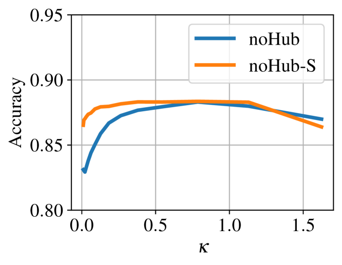
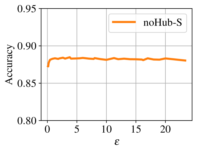
Figure 6: Accuracy for different values for $\kappa$ and $\varepsilon$. Neither noHub nor noHub-S are particularly sensitive the the choice of these parameters.

E.1 Implementation details

This section covers the additional implementation details not provided in the main paper. These include the initialization of the embeddings in Algorithm 1, hyperparameters, additional transformations wherever required, the architectures used, and a note on accessing the code, datasets, and dataset splits.

Initialization and normalization.  Instead of a random initialization of our embeddings $Z_{0}$, we follow a PCA based initialization, as in [30]. The weights are computed using the cached features from the base classes, the support and query features are then transformed using these weights. This procedure is also fast as we do not need to compute the PCA weights on every episode. To ensure that the resulting features lie on the hypersphere after each gradient update in noHub and noHub-S, we re-normalize the embeddings using L2 normalization.

Hyperparameters.  noHub and noHub-S have the following hyperparameters.

• $P$ – perplexity for computing the $\kappa_{i}$.

• $T$ – number of iterations.

• $\alpha$ – tradeoff parameter in the loss (${\pazocal{L}}_{\mathrm{noHub}}=\alpha{\pazocal{L}}_{\mathrm{LSP}}+(1-\alpha){\pazocal{L}}_{\mathrm{Unif}}$).

• $\eta$ – learning rate for the Adam optimizer.

• $\kappa$ – concentration parameter for the embeddings.

• $\varepsilon$ – exaggeration of similarities between supports from different classes.

• $d$ – dimensionality of embeddings.

All hyperparameter values used in in noHub and noHub-S are given in Table 5

			mini		tiered		CUB
Arch.	Param.	Method	1-shot	5-shot	1-shot	5-shot	1-shot	5-shot
ResNet18	$P$	noHub	45	45	45	45	45	45
		noHub-S	45	45	40	45	45	45
	$T$	noHub	50	50	50	50	50	50
		noHub-S	150	150	150	150	150	150
	$\alpha$	noHub	0.2	0.2	0.2	0.2	0.2	0.2
		noHub-S	0.3	0.2	0.2	0.2	0.3	0.2
	$\eta$	noHub	0.1	0.1	0.1	0.1	0.1	0.1
		noHub-S	0.1	0.1	0.1	0.1	0.1	0.1
	$\kappa$	noHub	0.5	0.5	0.5	0.5	0.5	0.5
		noHub-S	0.5	0.5	0.5	0.5	0.5	0.5
	$\varepsilon$	noHub	–	–	–	–	–	–
		noHub-S	8	8	5	8	8	8
	$d$	noHub	400	400	400	400	400	400
		noHub-S	400	400	400	400	400	400
WideRes28-10	$P$	noHub	45	45	45	45	45	45
		noHub-S	45	45	40	35	45	30
	$T$	noHub	50	50	50	50	50	50
		noHub-S	150	150	150	150	150	150
	$\alpha$	noHub	0.2	0.2	0.2	0.2	0.2	0.2
		noHub-S	0.3	0.2	0.2	0.1	0.3	0.1
	$\eta$	noHub	0.1	0.1	0.1	0.1	0.1	0.1
		noHub-S	0.1	0.1	0.1	0.1	0.1	0.1
	$\kappa$	noHub	0.5	0.5	0.5	0.5	0.5	0.5
		noHub-S	0.5	0.5	0.5	0.2	0.5	0.2
	$\varepsilon$	noHub	–	–	–	–	–	–
		noHub-S	8	8	5	12	8	8
	$d$	noHub	400	400	400	400	400	400
		noHub-S	400	400	400	400	400	400

Table 5: Hyperparameter values used in our experiments.

Code.  The code for our experiments is available at: https://github.com/uitml/noHub

Data splits.  Details to access the datasets used with the requisite splits (both are consistent with [7]) are available in the code repository.

Base feature extractors.

• Resnet-18: As in [6, 7], we use the weights from [7]. The model is trained using a cross-entropy loss on the base classes.

• WideRes28-10: Following [37, 11], we use the weights from [37]. The model is pre-trained using a combination of cross-entropy and rotation prediction [42], and then fine-tuned with Manifold Mixup [43].

E.2 Results

FSL performance.  The complete lists of accuracies and hubness metrics for all embeddings, classifiers, and feature extractors, are given in Tables 6, 7, 8, and 9. The exhaustive results in these tables form the basis of Table 1, Table 2 and Table 3 in the main text. The two proposed approaches consistently outperform prior embeddings across several classifiers, feature extractors and datasets.

Effect of the $\kappa$ and $\varepsilon$ hyperparameters.  The plots in Figure 6 show accuracy on tiered $5$-shot with SIAMESE for increasing $\kappa$ and $\varepsilon$. Neither method is particularly sensitive to the choice of $\kappa$ and $\varepsilon$, and noHub-S is less sensitive to variations in $\kappa$, than noHub. Choosing $\kappa\in[0.5,1]$ and $\varepsilon\in[3,20]$ will result in high classification accuracy

			mini			tiered			CUB
			Acc	Skew	Hub. Occ.	Acc	Skew	Hub. Occ.	Acc	Skew	Hub. Occ.
Arch.	Clf.	Emb.
ResNet18	ILPC	None	64.07 (0.28)	1.411 (0.01)	0.408 (0.001)	75.5 (0.28)	1.213 (0.009)	0.41 (0.001)	76.06 (0.27)	0.886 (0.006)	0.34 (0.001)
		L2	69.28 (0.27)	0.966 (0.007)	0.298 (0.001)	77.84 (0.28)	0.811 (0.007)	0.267 (0.001)	79.91 (0.26)	0.688 (0.006)	0.236 (0.001)
		CL2	71.48 (0.27)	0.661 (0.005)	0.229 (0.001)	79.8 (0.27)	0.679 (0.006)	0.249 (0.001)	80.97 (0.26)	0.553 (0.005)	0.203 (0.001)
		ZN	71.48 (0.27)	0.677 (0.006)	0.227 (0.001)	79.95 (0.27)	0.694 (0.006)	0.263 (0.001)	81.49 (0.25)	0.57 (0.005)	0.217 (0.001)
		ReRep	65.49 (0.28)	3.688 (0.007)	0.559 (0.001)	76.75 (0.28)	3.61 (0.01)	0.55 (0.001)	77.73 (0.26)	3.563 (0.007)	0.512 (0.001)
		EASE	71.79 (0.28)	0.515 (0.005)	0.157 (0.001)	80.2 (0.27)	0.48 (0.005)	0.158 (0.001)	81.88 (0.25)	0.463 (0.004)	0.153 (0.001)
		TCPR	71.77 (0.28)	0.647 (0.005)	0.223 (0.001)	80.01 (0.28)	0.652 (0.006)	0.249 (0.001)	81.75 (0.25)	0.534 (0.004)	0.203 (0.001)
		noHub	73.18 (0.28)	0.308 (0.005)	0.094 (0.001)	80.76 (0.28)	0.296 (0.004)	0.101 (0.001)	82.74 (0.26)	0.32 (0.004)	0.112 (0.001)
		noHub-S	74.02 (0.28)	0.276 (0.004)	0.13 (0.001)	81.34 (0.27)	0.281 (0.004)	0.127 (0.001)	83.92 (0.25)	0.296 (0.003)	0.163 (0.001)
	LaplacianShot	None	68.92 (0.23)	1.341 (0.009)	0.408 (0.001)	76.43 (0.25)	1.214 (0.009)	0.41 (0.001)	79.17 (0.23)	0.887 (0.006)	0.34 (0.001)
		L2	69.3 (0.23)	0.945 (0.007)	0.302 (0.001)	77.2 (0.25)	0.808 (0.007)	0.265 (0.001)	79.65 (0.23)	0.682 (0.006)	0.236 (0.001)
		CL2	70.68 (0.23)	0.661 (0.005)	0.231 (0.001)	77.98 (0.24)	0.689 (0.006)	0.248 (0.001)	79.99 (0.22)	0.547 (0.005)	0.201 (0.001)
		ZN	70.51 (0.23)	0.688 (0.006)	0.233 (0.001)	77.51 (0.24)	0.697 (0.006)	0.264 (0.001)	79.86 (0.22)	0.564 (0.005)	0.217 (0.001)
		ReRep	72.75 (0.24)	3.653 (0.007)	0.548 (0.001)	78.95 (0.25)	3.605 (0.011)	0.549 (0.001)	82.38 (0.22)	3.565 (0.007)	0.512 (0.001)
		EASE	72.19 (0.23)	0.526 (0.005)	0.161 (0.001)	79.34 (0.24)	0.481 (0.005)	0.158 (0.001)	81.5 (0.22)	0.459 (0.004)	0.152 (0.001)
		TCPR	71.79 (0.23)	0.654 (0.005)	0.228 (0.001)	78.41 (0.24)	0.651 (0.005)	0.249 (0.001)	80.86 (0.22)	0.537 (0.004)	0.203 (0.001)
		noHub	73.63 (0.25)	0.305 (0.005)	0.094 (0.001)	80.84 (0.25)	0.3 (0.005)	0.101 (0.001)	83.23 (0.22)	0.318 (0.004)	0.112 (0.001)
		noHub-S	73.79 (0.25)	0.276 (0.004)	0.13 (0.001)	80.83 (0.25)	0.275 (0.004)	0.125 (0.001)	83.47 (0.22)	0.299 (0.003)	0.164 (0.001)
	ObliqueManifold	None	68.89 (0.23)	1.412 (0.01)	0.407 (0.001)	77.07 (0.25)	1.21 (0.009)	0.409 (0.001)	79.4 (0.22)	0.887 (0.006)	0.341 (0.001)
		L2	68.92 (0.23)	0.964 (0.007)	0.299 (0.001)	77.17 (0.25)	0.806 (0.007)	0.266 (0.001)	79.32 (0.22)	0.691 (0.006)	0.237 (0.001)
		CL2	70.86 (0.24)	0.66 (0.005)	0.228 (0.001)	78.92 (0.25)	0.68 (0.006)	0.249 (0.001)	80.29 (0.23)	0.547 (0.005)	0.202 (0.001)
		ZN	71.25 (0.24)	0.679 (0.006)	0.227 (0.001)	79.54 (0.25)	0.697 (0.006)	0.263 (0.001)	81.38 (0.23)	0.562 (0.005)	0.216 (0.001)
		ReRep	73.3 (0.25)	3.682 (0.007)	0.559 (0.001)	80.26 (0.26)	3.608 (0.01)	0.551 (0.001)	83.84 (0.23)	3.559 (0.008)	0.513 (0.001)
		EASE	68.4 (0.24)	0.516 (0.005)	0.156 (0.001)	77.33 (0.25)	0.477 (0.004)	0.158 (0.001)	79.03 (0.24)	0.461 (0.004)	0.152 (0.001)
		TCPR	70.74 (0.24)	0.646 (0.005)	0.223 (0.001)	78.92 (0.25)	0.649 (0.005)	0.249 (0.001)	80.18 (0.23)	0.537 (0.004)	0.204 (0.001)
		noHub	72.55 (0.26)	0.309 (0.005)	0.095 (0.001)	79.97 (0.26)	0.302 (0.005)	0.102 (0.001)	82.21 (0.24)	0.319 (0.004)	0.112 (0.001)
		noHub-S	74.24 (0.26)	0.274 (0.004)	0.13 (0.001)	80.84 (0.26)	0.282 (0.004)	0.127 (0.001)	83.67 (0.23)	0.294 (0.003)	0.162 (0.001)
	SIAMESE	None	20.0 (0.0)	1.345 (0.009)	0.407 (0.001)	20.0 (0.0)	1.222 (0.009)	0.41 (0.001)	20.0 (0.0)	0.885 (0.006)	0.339 (0.001)
		L2	73.77 (0.24)	0.949 (0.007)	0.301 (0.001)	80.46 (0.26)	0.811 (0.007)	0.265 (0.001)	83.1 (0.23)	0.691 (0.006)	0.237 (0.001)
		CL2	75.56 (0.26)	0.666 (0.005)	0.232 (0.001)	82.1 (0.26)	0.68 (0.006)	0.248 (0.001)	84.35 (0.24)	0.549 (0.005)	0.201 (0.001)
		ZN	20.0 (0.0)	0.686 (0.006)	0.232 (0.001)	20.0 (0.0)	0.69 (0.006)	0.262 (0.001)	20.0 (0.0)	0.565 (0.005)	0.217 (0.001)
		ReRep	20.0 (0.0)	3.653 (0.007)	0.549 (0.001)	20.0 (0.0)	3.616 (0.01)	0.549 (0.001)	20.0 (0.0)	3.559 (0.007)	0.512 (0.001)
		EASE	76.05 (0.27)	0.529 (0.005)	0.162 (0.001)	82.57 (0.27)	0.485 (0.005)	0.159 (0.001)	85.24 (0.24)	0.464 (0.004)	0.153 (0.001)
		TCPR	75.99 (0.26)	0.655 (0.005)	0.227 (0.001)	82.65 (0.26)	0.651 (0.005)	0.249 (0.001)	85.34 (0.23)	0.535 (0.004)	0.203 (0.001)
		noHub	76.65 (0.28)	0.308 (0.005)	0.095 (0.001)	82.94 (0.27)	0.303 (0.004)	0.101 (0.001)	85.88 (0.24)	0.322 (0.004)	0.112 (0.001)
		noHub-S	76.68 (0.28)	0.275 (0.004)	0.13 (0.001)	83.09 (0.27)	0.281 (0.004)	0.128 (0.001)	85.81 (0.24)	0.295 (0.003)	0.161 (0.001)
	SimpleShot	None	56.14 (0.2)	1.349 (0.009)	0.407 (0.001)	63.34 (0.23)	1.211 (0.009)	0.408 (0.001)	64.02 (0.21)	0.887 (0.006)	0.341 (0.001)
		L2	60.15 (0.2)	0.937 (0.007)	0.301 (0.001)	68.02 (0.23)	0.812 (0.007)	0.265 (0.001)	69.05 (0.21)	0.691 (0.006)	0.236 (0.001)
		CL2	63.1 (0.2)	0.667 (0.005)	0.233 (0.001)	69.76 (0.22)	0.679 (0.006)	0.249 (0.001)	70.16 (0.2)	0.549 (0.005)	0.201 (0.001)
		ZN	63.39 (0.2)	0.68 (0.005)	0.231 (0.001)	70.04 (0.22)	0.698 (0.006)	0.264 (0.001)	71.03 (0.2)	0.564 (0.005)	0.216 (0.001)
		ReRep	66.66 (0.22)	3.655 (0.007)	0.548 (0.001)	73.23 (0.23)	3.604 (0.01)	0.549 (0.001)	76.8 (0.21)	3.565 (0.007)	0.513 (0.001)
		EASE	64.0 (0.2)	0.521 (0.005)	0.16 (0.001)	71.0 (0.21)	0.479 (0.005)	0.158 (0.001)	72.38 (0.2)	0.466 (0.004)	0.153 (0.001)
		TCPR	63.33 (0.2)	0.651 (0.005)	0.228 (0.001)	69.82 (0.22)	0.65 (0.005)	0.25 (0.001)	70.75 (0.2)	0.532 (0.004)	0.204 (0.001)
		noHub	69.38 (0.22)	0.315 (0.005)	0.095 (0.001)	76.72 (0.23)	0.303 (0.004)	0.102 (0.001)	78.21 (0.21)	0.32 (0.004)	0.112 (0.001)
		noHub-S	71.1 (0.22)	0.276 (0.004)	0.13 (0.001)	78.35 (0.23)	0.283 (0.004)	0.127 (0.001)	80.31 (0.21)	0.296 (0.003)	0.162 (0.001)
	$\alpha$-TIM	None	56.39 (0.2)	1.342 (0.009)	0.406 (0.001)	63.32 (0.23)	1.216 (0.009)	0.411 (0.001)	64.02 (0.22)	0.886 (0.006)	0.341 (0.001)
		L2	67.91 (0.23)	0.942 (0.007)	0.301 (0.001)	74.94 (0.24)	0.814 (0.007)	0.266 (0.001)	77.49 (0.23)	0.694 (0.006)	0.236 (0.001)
		CL2	65.68 (0.21)	0.665 (0.005)	0.232 (0.001)	73.23 (0.23)	0.681 (0.006)	0.248 (0.001)	73.79 (0.21)	0.552 (0.005)	0.202 (0.001)
		ZN	63.36 (0.2)	0.682 (0.005)	0.232 (0.001)	70.19 (0.22)	0.693 (0.006)	0.263 (0.001)	70.85 (0.21)	0.566 (0.005)	0.215 (0.001)
		ReRep	66.37 (0.22)	3.656 (0.007)	0.55 (0.001)	73.24 (0.24)	3.605 (0.011)	0.55 (0.001)	76.86 (0.21)	3.555 (0.007)	0.514 (0.001)
		EASE	65.32 (0.2)	0.526 (0.005)	0.163 (0.001)	71.88 (0.22)	0.477 (0.005)	0.158 (0.001)	73.03 (0.21)	0.459 (0.004)	0.151 (0.001)
		TCPR	66.19 (0.21)	0.65 (0.005)	0.227 (0.001)	73.24 (0.23)	0.649 (0.005)	0.25 (0.001)	74.07 (0.21)	0.532 (0.004)	0.203 (0.001)
		noHub	70.08 (0.23)	0.312 (0.005)	0.094 (0.001)	77.39 (0.24)	0.304 (0.004)	0.101 (0.001)	79.19 (0.22)	0.319 (0.004)	0.112 (0.001)
		noHub-S	72.04 (0.23)	0.273 (0.004)	0.13 (0.001)	79.13 (0.24)	0.282 (0.004)	0.126 (0.001)	81.42 (0.22)	0.296 (0.003)	0.161 (0.001)

Table 6: Resnet-18: 1-shot

			mini			tiered			CUB
			Acc	Skew	Hub. Occ.	Acc	Skew	Hub. Occ.	Acc	Skew	Hub. Occ.
Arch.	Clf.	Emb.
WideRes28-10	ILPC	None	71.27 (0.28)	1.595 (0.01)	0.46 (0.001)	75.01 (0.28)	1.807 (0.01)	0.494 (0.001)	89.75 (0.19)	1.072 (0.009)	0.367 (0.001)
		L2	76.41 (0.26)	0.773 (0.006)	0.295 (0.001)	78.25 (0.27)	0.731 (0.006)	0.274 (0.001)	90.27 (0.2)	0.473 (0.004)	0.228 (0.001)
		CL2	74.13 (0.27)	0.993 (0.009)	0.29 (0.001)	78.2 (0.27)	0.815 (0.006)	0.306 (0.001)	90.34 (0.2)	0.524 (0.004)	0.267 (0.001)
		ZN	77.76 (0.26)	0.728 (0.005)	0.287 (0.001)	79.42 (0.27)	0.776 (0.006)	0.302 (0.001)	90.21 (0.2)	0.516 (0.004)	0.263 (0.001)
		ReRep	62.51 (0.34)	3.56 (0.002)	0.704 (0.001)	60.66 (0.37)	3.55 (0.002)	0.776 (0.001)	87.44 (0.25)	3.033 (0.008)	0.472 (0.001)
		EASE	78.01 (0.26)	0.47 (0.004)	0.176 (0.001)	79.64 (0.27)	0.479 (0.004)	0.175 (0.001)	90.76 (0.19)	0.437 (0.003)	0.212 (0.001)
		TCPR	78.37 (0.26)	0.584 (0.005)	0.237 (0.001)	79.55 (0.28)	0.683 (0.006)	0.265 (0.001)	90.77 (0.19)	0.476 (0.004)	0.23 (0.001)
		noHub	78.84 (0.27)	0.293 (0.004)	0.112 (0.001)	80.75 (0.28)	0.3 (0.004)	0.112 (0.001)	90.91 (0.2)	0.189 (0.004)	0.109 (0.001)
		noHub-S	79.77 (0.26)	0.262 (0.004)	0.148 (0.001)	81.24 (0.27)	0.278 (0.004)	0.135 (0.001)	91.28 (0.19)	0.16 (0.004)	0.13 (0.001)
	LaplacianShot	None	72.56 (0.23)	1.599 (0.01)	0.459 (0.001)	75.58 (0.25)	1.795 (0.01)	0.495 (0.001)	88.71 (0.19)	1.071 (0.009)	0.369 (0.001)
		L2	75.18 (0.23)	0.777 (0.006)	0.296 (0.001)	77.03 (0.24)	0.732 (0.006)	0.274 (0.001)	89.73 (0.17)	0.474 (0.004)	0.229 (0.001)
		CL2	71.29 (0.24)	0.987 (0.009)	0.29 (0.001)	75.42 (0.25)	0.819 (0.006)	0.309 (0.001)	89.61 (0.18)	0.52 (0.004)	0.268 (0.001)
		ZN	75.18 (0.22)	0.724 (0.005)	0.286 (0.001)	77.0 (0.24)	0.768 (0.006)	0.301 (0.001)	89.22 (0.18)	0.517 (0.004)	0.263 (0.001)
		ReRep	75.25 (0.22)	3.562 (0.002)	0.704 (0.001)	77.12 (0.24)	3.548 (0.002)	0.776 (0.001)	88.98 (0.18)	3.024 (0.008)	0.47 (0.001)
		EASE	77.29 (0.22)	0.473 (0.004)	0.177 (0.001)	78.97 (0.24)	0.475 (0.004)	0.175 (0.001)	90.06 (0.17)	0.435 (0.003)	0.213 (0.001)
		TCPR	76.77 (0.22)	0.593 (0.005)	0.236 (0.001)	77.49 (0.24)	0.686 (0.006)	0.264 (0.001)	89.42 (0.17)	0.475 (0.004)	0.231 (0.001)
		noHub	79.13 (0.23)	0.29 (0.004)	0.111 (0.001)	80.5 (0.25)	0.302 (0.004)	0.112 (0.001)	90.73 (0.18)	0.19 (0.004)	0.109 (0.001)
		noHub-S	79.13 (0.23)	0.259 (0.004)	0.147 (0.001)	80.59 (0.24)	0.277 (0.004)	0.135 (0.001)	90.61 (0.17)	0.164 (0.004)	0.13 (0.001)
	ObliqueManifold	None	76.02 (0.22)	1.599 (0.01)	0.46 (0.001)	77.75 (0.25)	1.801 (0.01)	0.494 (0.001)	90.82 (0.18)	1.07 (0.009)	0.368 (0.001)
		L2	76.11 (0.22)	0.779 (0.006)	0.295 (0.001)	77.74 (0.25)	0.731 (0.006)	0.274 (0.001)	90.89 (0.18)	0.475 (0.004)	0.228 (0.001)
		CL2	74.43 (0.24)	0.985 (0.009)	0.289 (0.001)	77.98 (0.25)	0.816 (0.007)	0.307 (0.001)	90.6 (0.18)	0.523 (0.004)	0.267 (0.001)
		ZN	77.69 (0.23)	0.724 (0.005)	0.286 (0.001)	79.32 (0.24)	0.767 (0.006)	0.301 (0.001)	90.73 (0.18)	0.519 (0.004)	0.263 (0.001)
		ReRep	78.08 (0.23)	3.56 (0.002)	0.703 (0.001)	79.46 (0.25)	3.549 (0.002)	0.777 (0.001)	91.16 (0.18)	3.032 (0.008)	0.471 (0.001)
		EASE	74.77 (0.23)	0.472 (0.004)	0.178 (0.001)	77.07 (0.25)	0.473 (0.004)	0.174 (0.001)	89.2 (0.18)	0.439 (0.003)	0.212 (0.001)
		TCPR	77.39 (0.23)	0.587 (0.005)	0.236 (0.001)	78.75 (0.24)	0.687 (0.006)	0.265 (0.001)	89.93 (0.19)	0.474 (0.004)	0.23 (0.001)
		noHub	78.44 (0.24)	0.292 (0.004)	0.112 (0.001)	79.99 (0.26)	0.302 (0.004)	0.113 (0.001)	90.59 (0.19)	0.185 (0.004)	0.108 (0.001)
		noHub-S	79.89 (0.24)	0.259 (0.004)	0.148 (0.001)	80.67 (0.26)	0.279 (0.004)	0.137 (0.001)	91.37 (0.18)	0.162 (0.004)	0.13 (0.001)
	SIAMESE	None	45.69 (0.31)	1.594 (0.009)	0.459 (0.001)	75.29 (0.28)	1.801 (0.01)	0.495 (0.001)	61.36 (0.55)	1.074 (0.009)	0.37 (0.001)
		L2	80.2 (0.23)	0.776 (0.006)	0.296 (0.001)	80.89 (0.26)	0.735 (0.006)	0.275 (0.001)	91.98 (0.18)	0.476 (0.004)	0.23 (0.001)
		CL2	75.23 (0.27)	0.988 (0.009)	0.289 (0.001)	79.59 (0.27)	0.82 (0.006)	0.307 (0.001)	92.17 (0.18)	0.518 (0.004)	0.266 (0.001)
		ZN	20.0 (0.0)	0.726 (0.005)	0.286 (0.001)	20.0 (0.0)	0.775 (0.006)	0.302 (0.001)	20.0 (0.0)	0.517 (0.004)	0.264 (0.001)
		ReRep	36.69 (0.28)	3.561 (0.002)	0.705 (0.001)	67.41 (0.29)	3.55 (0.002)	0.776 (0.001)	57.62 (0.56)	3.027 (0.008)	0.472 (0.001)
		EASE	81.19 (0.25)	0.474 (0.004)	0.178 (0.001)	82.04 (0.26)	0.476 (0.004)	0.176 (0.001)	91.99 (0.19)	0.436 (0.003)	0.213 (0.001)
		TCPR	81.27 (0.24)	0.582 (0.005)	0.236 (0.001)	81.89 (0.26)	0.681 (0.006)	0.264 (0.001)	91.91 (0.18)	0.477 (0.004)	0.232 (0.001)
		noHub	81.97 (0.25)	0.291 (0.004)	0.111 (0.001)	82.8 (0.27)	0.298 (0.004)	0.112 (0.001)	92.53 (0.18)	0.189 (0.004)	0.109 (0.001)
		noHub-S	82.0 (0.26)	0.258 (0.004)	0.148 (0.001)	82.85 (0.27)	0.278 (0.004)	0.137 (0.001)	92.63 (0.18)	0.159 (0.004)	0.13 (0.001)
	SimpleShot	None	55.66 (0.21)	1.6 (0.01)	0.459 (0.001)	54.71 (0.22)	1.81 (0.01)	0.494 (0.001)	70.92 (0.23)	1.073 (0.009)	0.369 (0.001)
		L2	65.78 (0.2)	0.781 (0.006)	0.296 (0.001)	68.75 (0.22)	0.737 (0.006)	0.275 (0.001)	82.85 (0.19)	0.475 (0.004)	0.228 (0.001)
		CL2	64.33 (0.2)	0.981 (0.009)	0.288 (0.001)	67.66 (0.22)	0.817 (0.006)	0.307 (0.001)	82.8 (0.19)	0.52 (0.004)	0.267 (0.001)
		ZN	67.31 (0.2)	0.73 (0.005)	0.287 (0.001)	69.14 (0.22)	0.769 (0.006)	0.302 (0.001)	82.79 (0.19)	0.517 (0.004)	0.263 (0.001)
		ReRep	67.38 (0.2)	3.56 (0.002)	0.704 (0.001)	70.17 (0.22)	3.55 (0.002)	0.777 (0.001)	84.86 (0.19)	3.026 (0.008)	0.47 (0.001)
		EASE	68.62 (0.2)	0.47 (0.004)	0.177 (0.001)	70.26 (0.21)	0.477 (0.004)	0.175 (0.001)	84.14 (0.18)	0.437 (0.003)	0.213 (0.001)
		TCPR	68.45 (0.2)	0.589 (0.005)	0.236 (0.001)	68.68 (0.22)	0.685 (0.006)	0.264 (0.001)	82.28 (0.19)	0.477 (0.004)	0.231 (0.001)
		noHub	75.06 (0.21)	0.29 (0.004)	0.111 (0.001)	76.7 (0.23)	0.301 (0.004)	0.111 (0.001)	88.06 (0.18)	0.188 (0.004)	0.108 (0.001)
		noHub-S	76.86 (0.21)	0.258 (0.004)	0.148 (0.001)	78.4 (0.23)	0.274 (0.004)	0.135 (0.001)	89.25 (0.18)	0.162 (0.004)	0.13 (0.001)
	$\alpha$-TIM	None	60.31 (0.2)	1.603 (0.01)	0.458 (0.001)	69.42 (0.25)	1.811 (0.01)	0.494 (0.001)	73.83 (0.21)	1.072 (0.009)	0.369 (0.001)
		L2	72.11 (0.22)	0.778 (0.006)	0.295 (0.001)	74.45 (0.23)	0.73 (0.006)	0.275 (0.001)	85.96 (0.19)	0.476 (0.004)	0.229 (0.001)
		CL2	68.5 (0.21)	0.988 (0.009)	0.29 (0.001)	72.17 (0.23)	0.811 (0.006)	0.306 (0.001)	85.6 (0.18)	0.522 (0.004)	0.267 (0.001)
		ZN	67.69 (0.2)	0.73 (0.005)	0.287 (0.001)	68.94 (0.22)	0.769 (0.006)	0.302 (0.001)	83.03 (0.19)	0.518 (0.004)	0.263 (0.001)
		ReRep	73.15 (0.23)	3.56 (0.002)	0.704 (0.001)	76.19 (0.25)	3.551 (0.002)	0.778 (0.001)	88.55 (0.18)	3.027 (0.008)	0.472 (0.001)
		EASE	69.83 (0.2)	0.468 (0.004)	0.176 (0.001)	71.54 (0.22)	0.481 (0.004)	0.175 (0.001)	84.9 (0.19)	0.436 (0.003)	0.213 (0.001)
		TCPR	71.6 (0.21)	0.586 (0.005)	0.237 (0.001)	72.71 (0.22)	0.689 (0.006)	0.264 (0.001)	84.99 (0.19)	0.479 (0.004)	0.231 (0.001)
		noHub	75.87 (0.22)	0.29 (0.004)	0.111 (0.001)	77.83 (0.23)	0.302 (0.004)	0.112 (0.001)	88.7 (0.17)	0.189 (0.004)	0.108 (0.001)
		noHub-S	77.76 (0.22)	0.259 (0.004)	0.147 (0.001)	79.04 (0.24)	0.276 (0.004)	0.136 (0.001)	89.77 (0.17)	0.163 (0.003)	0.13 (0.001)

Table 7: WideRes28-10: 1-shot

			mini			tiered			CUB
			Acc	Skew	Hub. Occ.	Acc	Skew	Hub. Occ.	Acc	Skew	Hub. Occ.
Arch.	Clf.	Emb.
ResNet18	ILPC	None	76.46 (0.18)	1.503 (0.01)	0.421 (0.001)	84.46 (0.18)	1.334 (0.008)	0.433 (0.001)	85.86 (0.14)	0.981 (0.005)	0.364 (0.001)
		L2	80.9 (0.16)	1.051 (0.007)	0.314 (0.001)	86.23 (0.17)	0.912 (0.006)	0.289 (0.001)	88.03 (0.13)	0.808 (0.005)	0.264 (0.001)
		CL2	81.64 (0.16)	0.778 (0.005)	0.262 (0.001)	86.88 (0.17)	0.823 (0.006)	0.281 (0.001)	88.44 (0.13)	0.695 (0.005)	0.235 (0.001)
		ZN	81.61 (0.16)	0.793 (0.005)	0.258 (0.001)	86.9 (0.17)	0.841 (0.006)	0.297 (0.001)	88.44 (0.12)	0.717 (0.004)	0.25 (0.001)
		ReRep	74.83 (0.19)	1.623 (0.003)	0.871 (0.001)	83.96 (0.19)	1.722 (0.004)	0.873 (0.001)	84.54 (0.15)	1.432 (0.003)	0.869 (0.001)
		EASE	81.75 (0.16)	0.618 (0.005)	0.182 (0.001)	86.84 (0.17)	0.593 (0.004)	0.181 (0.001)	88.85 (0.12)	0.606 (0.004)	0.186 (0.001)
		TCPR	81.76 (0.16)	0.766 (0.005)	0.254 (0.001)	86.78 (0.17)	0.801 (0.005)	0.284 (0.001)	88.69 (0.13)	0.683 (0.004)	0.237 (0.001)
		noHub	82.09 (0.16)	0.295 (0.004)	0.097 (0.001)	86.81 (0.17)	0.289 (0.004)	0.102 (0.001)	88.85 (0.13)	0.333 (0.004)	0.12 (0.001)
		noHub-S	82.33 (0.16)	0.488 (0.006)	0.086 (0.001)	87.05 (0.17)	0.475 (0.006)	0.091 (0.001)	89.12 (0.13)	0.438 (0.006)	0.097 (0.001)
	LaplacianShot	None	81.97 (0.15)	1.442 (0.009)	0.422 (0.001)	86.17 (0.16)	1.336 (0.008)	0.432 (0.001)	88.58 (0.12)	0.985 (0.005)	0.365 (0.001)
		L2	81.89 (0.14)	1.035 (0.007)	0.319 (0.001)	86.19 (0.16)	0.913 (0.006)	0.289 (0.001)	88.52 (0.11)	0.811 (0.005)	0.264 (0.001)
		CL2	81.93 (0.14)	0.786 (0.005)	0.265 (0.001)	86.16 (0.16)	0.82 (0.006)	0.282 (0.001)	88.46 (0.12)	0.7 (0.005)	0.235 (0.001)
		ZN	82.57 (0.14)	0.803 (0.005)	0.263 (0.001)	86.67 (0.16)	0.838 (0.006)	0.296 (0.001)	88.88 (0.11)	0.714 (0.004)	0.25 (0.001)
		ReRep	82.32 (0.14)	1.633 (0.003)	0.863 (0.001)	86.09 (0.16)	1.721 (0.004)	0.873 (0.001)	88.74 (0.12)	1.431 (0.002)	0.869 (0.001)
		EASE	82.57 (0.14)	0.627 (0.005)	0.186 (0.001)	86.82 (0.15)	0.596 (0.004)	0.182 (0.001)	88.94 (0.11)	0.608 (0.004)	0.185 (0.001)
		TCPR	82.24 (0.14)	0.781 (0.005)	0.259 (0.001)	86.27 (0.16)	0.797 (0.005)	0.284 (0.001)	88.63 (0.11)	0.687 (0.004)	0.236 (0.001)
		noHub	82.55 (0.15)	0.285 (0.004)	0.096 (0.001)	86.75 (0.16)	0.29 (0.004)	0.103 (0.001)	89.08 (0.11)	0.329 (0.004)	0.12 (0.001)
		noHub-S	82.81 (0.14)	0.25 (0.005)	0.073 (0.001)	87.12 (0.16)	0.214 (0.005)	0.077 (0.001)	88.99 (0.11)	0.438 (0.006)	0.096 (0.001)
	ObliqueManifold	None	83.53 (0.15)	1.497 (0.01)	0.421 (0.001)	87.85 (0.15)	1.334 (0.009)	0.433 (0.001)	90.28 (0.11)	0.987 (0.005)	0.364 (0.001)
		L2	83.66 (0.15)	1.051 (0.007)	0.314 (0.001)	87.83 (0.15)	0.922 (0.006)	0.289 (0.001)	90.21 (0.11)	0.81 (0.005)	0.263 (0.001)
		CL2	83.62 (0.15)	0.775 (0.005)	0.261 (0.001)	88.1 (0.15)	0.823 (0.006)	0.281 (0.001)	90.09 (0.11)	0.701 (0.005)	0.236 (0.001)
		ZN	83.86 (0.15)	0.795 (0.005)	0.258 (0.001)	88.47 (0.15)	0.835 (0.006)	0.296 (0.001)	90.47 (0.11)	0.716 (0.004)	0.251 (0.001)
		ReRep	82.44 (0.15)	1.62 (0.003)	0.871 (0.001)	86.85 (0.16)	1.725 (0.004)	0.872 (0.001)	89.83 (0.11)	1.431 (0.003)	0.869 (0.001)
		EASE	82.83 (0.15)	0.628 (0.005)	0.185 (0.001)	87.63 (0.16)	0.597 (0.005)	0.182 (0.001)	89.74 (0.12)	0.609 (0.004)	0.186 (0.001)
		TCPR	83.51 (0.15)	0.766 (0.005)	0.255 (0.001)	88.09 (0.15)	0.795 (0.005)	0.283 (0.001)	90.28 (0.11)	0.687 (0.004)	0.236 (0.001)
		noHub	83.28 (0.15)	0.287 (0.004)	0.096 (0.001)	87.58 (0.16)	0.288 (0.004)	0.102 (0.001)	89.89 (0.12)	0.334 (0.004)	0.121 (0.001)
		noHub-S	83.25 (0.16)	0.487 (0.006)	0.086 (0.001)	87.82 (0.16)	0.469 (0.006)	0.091 (0.001)	89.38 (0.17)	nan (nan)	0.097 (0.001)
	SIAMESE	None	20.0 (0.0)	1.441 (0.009)	0.421 (0.001)	20.0 (0.0)	1.339 (0.009)	0.433 (0.001)	20.0 (0.0)	0.984 (0.005)	0.364 (0.001)
		L2	83.14 (0.14)	1.035 (0.007)	0.319 (0.001)	87.04 (0.16)	0.912 (0.006)	0.288 (0.001)	89.48 (0.12)	0.808 (0.005)	0.264 (0.001)
		CL2	84.04 (0.15)	0.788 (0.005)	0.264 (0.001)	87.9 (0.16)	0.816 (0.006)	0.28 (0.001)	90.14 (0.12)	0.698 (0.005)	0.235 (0.001)
		ZN	20.0 (0.0)	0.8 (0.005)	0.263 (0.001)	20.0 (0.0)	0.84 (0.006)	0.296 (0.001)	20.0 (0.0)	0.713 (0.004)	0.251 (0.001)
		ReRep	20.0 (0.0)	1.633 (0.003)	0.863 (0.001)	20.0 (0.0)	1.724 (0.004)	0.872 (0.001)	20.0 (0.0)	1.428 (0.002)	0.869 (0.001)
		EASE	84.61 (0.15)	0.63 (0.005)	0.187 (0.001)	88.33 (0.16)	0.594 (0.004)	0.182 (0.001)	90.42 (0.12)	0.607 (0.004)	0.185 (0.001)
		TCPR	84.39 (0.15)	0.772 (0.005)	0.259 (0.001)	88.26 (0.16)	0.791 (0.005)	0.283 (0.001)	90.5 (0.11)	0.686 (0.004)	0.235 (0.001)
		noHub	84.05 (0.16)	0.292 (0.004)	0.096 (0.001)	87.87 (0.17)	0.291 (0.004)	0.103 (0.001)	90.34 (0.12)	0.334 (0.004)	0.12 (0.001)
		noHub-S	84.67 (0.15)	0.247 (0.005)	0.074 (0.001)	88.43 (0.16)	0.473 (0.006)	0.092 (0.001)	90.52 (0.12)	0.443 (0.006)	0.097 (0.001)
	SimpleShot	None	78.5 (0.14)	1.436 (0.009)	0.422 (0.001)	83.95 (0.16)	1.339 (0.008)	0.432 (0.001)	85.65 (0.12)	0.987 (0.005)	0.364 (0.001)
		L2	79.89 (0.14)	1.04 (0.007)	0.318 (0.001)	84.5 (0.16)	0.914 (0.006)	0.287 (0.001)	86.46 (0.12)	0.812 (0.005)	0.263 (0.001)
		CL2	80.0 (0.14)	0.786 (0.005)	0.264 (0.001)	84.66 (0.16)	0.821 (0.006)	0.28 (0.001)	86.3 (0.12)	0.698 (0.005)	0.236 (0.001)
		ZN	80.57 (0.14)	0.806 (0.005)	0.264 (0.001)	84.97 (0.16)	0.839 (0.006)	0.296 (0.001)	86.76 (0.12)	0.716 (0.005)	0.25 (0.001)
		ReRep	80.86 (0.14)	1.631 (0.003)	0.863 (0.001)	85.05 (0.16)	1.721 (0.004)	0.872 (0.001)	87.83 (0.12)	1.432 (0.002)	0.869 (0.001)
		EASE	80.13 (0.14)	0.624 (0.005)	0.186 (0.001)	84.74 (0.16)	0.598 (0.004)	0.183 (0.001)	86.76 (0.12)	0.607 (0.004)	0.186 (0.001)
		TCPR	80.15 (0.14)	0.78 (0.005)	0.259 (0.001)	84.86 (0.15)	0.796 (0.005)	0.283 (0.001)	86.8 (0.12)	0.687 (0.004)	0.235 (0.001)
		noHub	82.13 (0.14)	0.286 (0.004)	0.096 (0.001)	86.31 (0.16)	0.289 (0.004)	0.104 (0.001)	88.46 (0.11)	0.329 (0.004)	0.12 (0.001)
		noHub-S	81.22 (0.14)	0.25 (0.005)	0.074 (0.001)	86.22 (0.15)	0.213 (0.005)	0.078 (0.001)	87.6 (0.12)	0.433 (0.006)	0.097 (0.001)
	$\alpha$-TIM	None	78.51 (0.15)	1.45 (0.009)	0.42 (0.001)	83.86 (0.16)	1.341 (0.009)	0.433 (0.001)	85.7 (0.12)	0.981 (0.005)	0.363 (0.001)
		L2	80.02 (0.16)	1.036 (0.007)	0.318 (0.001)	84.49 (0.18)	0.92 (0.006)	0.288 (0.001)	87.88 (0.13)	0.812 (0.005)	0.264 (0.001)
		CL2	80.46 (0.16)	0.784 (0.005)	0.264 (0.001)	84.86 (0.17)	0.82 (0.006)	0.281 (0.001)	87.53 (0.13)	0.701 (0.005)	0.235 (0.001)
		ZN	80.32 (0.14)	0.802 (0.005)	0.263 (0.001)	84.93 (0.16)	0.834 (0.006)	0.295 (0.001)	86.95 (0.12)	0.715 (0.004)	0.25 (0.001)
		ReRep	81.05 (0.14)	1.63 (0.003)	0.863 (0.001)	85.18 (0.16)	1.718 (0.004)	0.872 (0.001)	87.63 (0.12)	1.43 (0.002)	0.87 (0.001)
		EASE	79.13 (0.15)	0.632 (0.005)	0.188 (0.001)	84.04 (0.17)	0.596 (0.004)	0.181 (0.001)	86.7 (0.13)	0.607 (0.004)	0.186 (0.001)
		TCPR	80.52 (0.16)	0.776 (0.005)	0.259 (0.001)	85.01 (0.17)	0.796 (0.005)	0.283 (0.001)	87.81 (0.13)	0.681 (0.004)	0.234 (0.001)
		noHub	81.39 (0.15)	0.29 (0.004)	0.096 (0.001)	86.09 (0.16)	0.292 (0.004)	0.103 (0.001)	88.16 (0.12)	0.336 (0.004)	0.121 (0.001)
		noHub-S	81.37 (0.15)	0.253 (0.005)	0.074 (0.001)	86.14 (0.16)	0.219 (0.005)	0.078 (0.001)	87.97 (0.12)	0.437 (0.006)	0.096 (0.001)

Table 8: Resnet-18: 5-shot

			mini			tiered			CUB
			Acc	Skew	Hub. Occ.	Acc	Skew	Hub. Occ.	Acc	Skew	Hub. Occ.
Arch.	Clf.	Emb.
WideRes28-10	ILPC	None	81.93 (0.16)	1.717 (0.01)	0.473 (0.001)	84.34 (0.17)	1.927 (0.011)	0.509 (0.001)	93.18 (0.11)	1.164 (0.008)	0.396 (0.001)
		L2	85.74 (0.14)	0.888 (0.005)	0.322 (0.001)	86.26 (0.17)	0.859 (0.005)	0.306 (0.001)	93.77 (0.1)	0.636 (0.004)	0.266 (0.001)
		CL2	83.33 (0.16)	1.12 (0.009)	0.318 (0.001)	85.99 (0.17)	0.957 (0.006)	0.338 (0.001)	93.79 (0.1)	0.703 (0.004)	0.309 (0.001)
		ZN	85.96 (0.14)	0.858 (0.005)	0.32 (0.001)	86.77 (0.16)	0.909 (0.006)	0.335 (0.001)	93.73 (0.1)	0.696 (0.004)	0.305 (0.001)
		ReRep	72.11 (0.27)	1.601 (0.003)	0.819 (0.001)	71.68 (0.3)	1.616 (0.004)	0.845 (0.001)	91.52 (0.13)	1.301 (0.005)	0.548 (0.002)
		EASE	85.89 (0.14)	0.577 (0.004)	0.198 (0.001)	86.83 (0.17)	0.583 (0.004)	0.193 (0.001)	93.87 (0.1)	0.576 (0.004)	0.242 (0.001)
		TCPR	86.29 (0.14)	0.715 (0.004)	0.27 (0.001)	86.96 (0.17)	0.819 (0.005)	0.295 (0.001)	93.82 (0.1)	0.634 (0.004)	0.265 (0.001)
		noHub	86.07 (0.15)	0.295 (0.004)	0.115 (0.001)	86.75 (0.17)	0.299 (0.004)	0.115 (0.001)	93.72 (0.1)	0.2 (0.004)	0.101 (0.001)
		noHub-S	86.41 (0.14)	0.499 (0.006)	0.104 (0.001)	87.31 (0.17)	0.406 (0.005)	0.121 (0.001)	93.79 (0.1)	0.416 (0.005)	0.126 (0.001)
	LaplacianShot	None	85.23 (0.13)	1.711 (0.01)	0.474 (0.001)	86.14 (0.15)	1.921 (0.011)	0.509 (0.001)	92.61 (0.1)	1.164 (0.008)	0.395 (0.001)
		L2	85.9 (0.13)	0.892 (0.006)	0.321 (0.001)	86.47 (0.15)	0.867 (0.006)	0.304 (0.001)	93.17 (0.09)	0.635 (0.004)	0.267 (0.001)
		CL2	82.08 (0.15)	1.112 (0.009)	0.318 (0.001)	84.62 (0.16)	0.954 (0.006)	0.34 (0.001)	93.01 (0.1)	0.702 (0.004)	0.309 (0.001)
		ZN	85.97 (0.13)	0.86 (0.005)	0.319 (0.001)	86.67 (0.15)	0.912 (0.006)	0.335 (0.001)	93.3 (0.1)	0.698 (0.004)	0.305 (0.001)
		ReRep	84.34 (0.14)	1.599 (0.003)	0.819 (0.001)	85.61 (0.16)	1.615 (0.004)	0.845 (0.001)	92.2 (0.1)	1.304 (0.005)	0.549 (0.002)
		EASE	86.24 (0.13)	0.573 (0.004)	0.198 (0.001)	86.74 (0.15)	0.582 (0.004)	0.194 (0.001)	93.31 (0.09)	0.578 (0.004)	0.243 (0.001)
		TCPR	86.16 (0.13)	0.712 (0.004)	0.269 (0.001)	85.72 (0.16)	0.813 (0.005)	0.293 (0.001)	92.99 (0.1)	0.638 (0.004)	0.264 (0.001)
		noHub	86.25 (0.13)	0.292 (0.004)	0.115 (0.001)	86.78 (0.16)	0.299 (0.004)	0.115 (0.001)	93.38 (0.09)	0.197 (0.004)	0.1 (0.001)
		noHub-S	85.79 (0.13)	0.494 (0.006)	0.103 (0.001)	86.44 (0.16)	0.397 (0.005)	0.12 (0.001)	93.36 (0.1)	0.42 (0.005)	0.126 (0.001)
	ObliqueManifold	None	87.46 (0.13)	1.712 (0.01)	0.472 (0.001)	88.16 (0.15)	1.913 (0.01)	0.509 (0.001)	94.75 (0.09)	1.161 (0.008)	0.395 (0.001)
		L2	87.61 (0.13)	0.889 (0.005)	0.321 (0.001)	88.14 (0.15)	0.862 (0.006)	0.306 (0.001)	94.8 (0.09)	0.642 (0.004)	0.268 (0.001)
		CL2	86.03 (0.14)	1.112 (0.009)	0.317 (0.001)	87.64 (0.16)	0.949 (0.006)	0.338 (0.001)	94.67 (0.09)	0.703 (0.004)	0.31 (0.001)
		ZN	87.88 (0.13)	0.852 (0.005)	0.32 (0.001)	88.43 (0.15)	0.908 (0.006)	0.335 (0.001)	94.77 (0.08)	0.697 (0.004)	0.306 (0.001)
		ReRep	87.62 (0.12)	1.599 (0.003)	0.819 (0.001)	88.15 (0.15)	1.616 (0.004)	0.845 (0.001)	94.48 (0.09)	1.302 (0.005)	0.547 (0.002)
		EASE	86.75 (0.13)	0.573 (0.004)	0.198 (0.001)	87.78 (0.15)	0.583 (0.004)	0.193 (0.001)	94.16 (0.09)	0.57 (0.004)	0.24 (0.001)
		TCPR	87.94 (0.12)	0.718 (0.004)	0.271 (0.001)	88.15 (0.15)	0.816 (0.005)	0.294 (0.001)	94.47 (0.09)	0.635 (0.004)	0.265 (0.001)
		noHub	87.23 (0.13)	0.297 (0.004)	0.115 (0.001)	87.95 (0.16)	0.296 (0.004)	0.114 (0.001)	94.13 (0.09)	0.197 (0.004)	0.1 (0.001)
		noHub-S	87.13 (0.14)	0.495 (0.006)	0.103 (0.001)	87.84 (0.16)	0.399 (0.005)	0.12 (0.001)	94.06 (0.09)	0.421 (0.005)	0.126 (0.001)
	SIAMESE	None	58.82 (0.31)	1.722 (0.01)	0.473 (0.001)	82.56 (0.22)	1.93 (0.01)	0.511 (0.001)	82.22 (0.37)	1.154 (0.008)	0.396 (0.001)
		L2	87.11 (0.13)	0.894 (0.006)	0.321 (0.001)	87.34 (0.15)	0.861 (0.005)	0.305 (0.001)	94.15 (0.1)	0.638 (0.004)	0.266 (0.001)
		CL2	83.99 (0.16)	1.107 (0.009)	0.318 (0.001)	86.71 (0.16)	0.953 (0.006)	0.339 (0.001)	94.48 (0.09)	0.704 (0.004)	0.31 (0.001)
		ZN	20.0 (0.0)	0.856 (0.005)	0.319 (0.001)	20.0 (0.0)	0.913 (0.006)	0.334 (0.001)	20.0 (0.0)	0.702 (0.004)	0.305 (0.001)
		ReRep	36.41 (0.3)	1.597 (0.003)	0.818 (0.001)	76.49 (0.24)	1.613 (0.004)	0.846 (0.001)	60.36 (0.6)	1.299 (0.005)	0.547 (0.002)
		EASE	87.82 (0.13)	0.579 (0.004)	0.199 (0.001)	88.06 (0.16)	0.586 (0.004)	0.192 (0.001)	94.36 (0.09)	0.571 (0.004)	0.241 (0.001)
		TCPR	87.8 (0.13)	0.717 (0.004)	0.27 (0.001)	87.95 (0.16)	0.822 (0.005)	0.295 (0.001)	94.25 (0.1)	0.637 (0.004)	0.266 (0.001)
		noHub	87.78 (0.14)	0.29 (0.004)	0.114 (0.001)	87.99 (0.17)	0.297 (0.004)	0.115 (0.001)	94.56 (0.09)	0.196 (0.004)	0.1 (0.001)
		noHub-S	88.03 (0.13)	0.492 (0.006)	0.103 (0.001)	88.31 (0.16)	0.398 (0.005)	0.12 (0.001)	94.69 (0.09)	0.416 (0.005)	0.127 (0.001)
	SimpleShot	None	78.56 (0.14)	1.709 (0.01)	0.473 (0.001)	80.32 (0.16)	1.937 (0.01)	0.51 (0.001)	89.27 (0.11)	1.16 (0.008)	0.395 (0.001)
		L2	83.81 (0.13)	0.887 (0.005)	0.322 (0.001)	84.82 (0.15)	0.86 (0.006)	0.305 (0.001)	92.06 (0.1)	0.632 (0.004)	0.266 (0.001)
		CL2	81.05 (0.14)	1.12 (0.009)	0.318 (0.001)	83.82 (0.16)	0.956 (0.006)	0.337 (0.001)	92.19 (0.1)	0.701 (0.004)	0.31 (0.001)
		ZN	83.92 (0.13)	0.858 (0.005)	0.32 (0.001)	85.1 (0.15)	0.912 (0.006)	0.335 (0.001)	92.17 (0.1)	0.699 (0.004)	0.305 (0.001)
		ReRep	79.26 (0.16)	1.597 (0.003)	0.819 (0.001)	82.7 (0.16)	1.617 (0.004)	0.846 (0.001)	91.48 (0.11)	1.299 (0.005)	0.549 (0.002)
		EASE	83.65 (0.13)	0.579 (0.004)	0.199 (0.001)	84.47 (0.15)	0.585 (0.004)	0.193 (0.001)	92.01 (0.1)	0.572 (0.004)	0.241 (0.001)
		TCPR	83.77 (0.13)	0.717 (0.004)	0.27 (0.001)	84.81 (0.15)	0.815 (0.005)	0.294 (0.001)	91.84 (0.1)	0.634 (0.004)	0.264 (0.001)
		noHub	85.73 (0.13)	0.294 (0.004)	0.115 (0.001)	86.58 (0.15)	0.298 (0.004)	0.115 (0.001)	93.21 (0.09)	0.195 (0.004)	0.1 (0.001)
		noHub-S	84.39 (0.13)	0.494 (0.006)	0.103 (0.001)	86.38 (0.15)	0.407 (0.005)	0.12 (0.001)	93.39 (0.09)	0.421 (0.005)	0.127 (0.001)
	$\alpha$-TIM	None	80.61 (0.15)	1.711 (0.01)	0.473 (0.001)	83.05 (0.18)	1.928 (0.01)	0.51 (0.001)	84.89 (0.29)	1.153 (0.008)	0.396 (0.001)
		L2	83.71 (0.16)	0.892 (0.005)	0.323 (0.001)	84.69 (0.18)	0.863 (0.005)	0.304 (0.001)	92.88 (0.1)	0.633 (0.004)	0.266 (0.001)
		CL2	82.35 (0.16)	1.111 (0.009)	0.318 (0.001)	84.06 (0.18)	0.949 (0.006)	0.339 (0.001)	92.81 (0.1)	0.7 (0.004)	0.31 (0.001)
		ZN	83.93 (0.13)	0.857 (0.005)	0.321 (0.001)	85.07 (0.15)	0.912 (0.006)	0.336 (0.001)	92.15 (0.1)	0.698 (0.004)	0.306 (0.001)
		ReRep	83.4 (0.14)	1.596 (0.003)	0.82 (0.001)	84.4 (0.16)	1.615 (0.004)	0.845 (0.001)	93.19 (0.09)	1.302 (0.005)	0.547 (0.002)
		EASE	82.72 (0.14)	0.576 (0.004)	0.2 (0.001)	83.86 (0.16)	0.583 (0.004)	0.193 (0.001)	92.31 (0.1)	0.572 (0.004)	0.242 (0.001)
		TCPR	84.21 (0.15)	0.718 (0.004)	0.27 (0.001)	84.63 (0.18)	0.814 (0.005)	0.293 (0.001)	92.44 (0.1)	0.635 (0.004)	0.265 (0.001)
		noHub	85.56 (0.13)	0.293 (0.004)	0.115 (0.001)	86.37 (0.16)	0.3 (0.004)	0.115 (0.001)	92.89 (0.1)	0.193 (0.004)	0.099 (0.001)
		noHub-S	83.96 (0.15)	0.496 (0.006)	0.102 (0.001)	86.01 (0.16)	0.395 (0.005)	0.12 (0.001)	93.24 (0.1)	0.422 (0.005)	0.126 (0.001)

Table 9: WideRes28-10: 5-shot

Appendix F Potential Negative Societal Impacts

As is the case with most methodological research in machine learning, the methods developed in this work could be used in downstream applications with potential negative societal impacts. Real world machine learning-based systems that interact with humans, or the environment in general, should therefore be properly tested and equipped with adequate safety measures.

Since our work relies on a large number of labeled examples from the base classes, un-discovered biases from the base dataset could be transferred to the trained models. Furthermore, the small number of examples in the inference stage could make the query predictions biased towards the included support examples, and not accurately reflect the diversity of the novel classes.

References

- He et al. [2016] Kaiming He, Xiangyu Zhang, Shaoqing Ren, and Jian Sun. Deep residual learning for image recognition. In CVPR, 2016.
- Dosovitskiy et al. [2021] Alexey Dosovitskiy, Lucas Beyer, Alexander Kolesnikov, Dirk Weissenborn, Xiaohua Zhai, Thomas Unterthiner, Mostafa Dehghani, Matthias Minderer, Georg Heigold, Sylvain Gelly, Jakob Uszkoreit, and Neil Houlsby. An image is worth 16x16 words: Transformers for image recognition at scale. In ICLR, 2021.
- Kim et al. [2019] Jongmin Kim, Taesup Kim, Sungwoong Kim, and Chang D Yoo. Edge-labeling graph neural network for few-shot learning. In CVPR, 2019.
- Wang et al. [2019] Yan Wang, Wei-Lun Chao, Kilian Q. Weinberger, and Laurens van der Maaten. SimpleShot: Revisiting Nearest-Neighbor Classification for Few-Shot Learning. arXiv:1911.04623 [cs], 2019.
- Ziko et al. [2020] Imtiaz Ziko, Jose Dolz, Eric Granger, and Ismail Ben Ayed. Laplacian Regularized Few-Shot Learning. In ICML, 2020.
- Boudiaf et al. [2020] Malik Boudiaf, Ziko Imtiaz Masud, Jérôme Rony, José Dolz, Pablo Piantanida, and Ismail Ben Ayed. Transductive Information Maximization For Few-Shot Learning. In NeurIPS, 2020.
- Veilleux et al. [2021] Olivier Veilleux, Malik Boudiaf, Pablo Piantanida, and Ismail Ben Ayed. Realistic evaluation of transductive few-shot learning. In NeurIPS, 2021.
- Qi et al. [2021] Guodong Qi, Huimin Yu, Zhaohui Lu, and Shuzhao Li. Transductive Few-Shot Classification on the Oblique Manifold. In ICCV, 2021.
- Lazarou et al. [2021] Michalis Lazarou, Tania Stathaki, and Yannis Avrithis. Iterative Label Cleaning for Transductive and Semi-Supervised Few-Shot Learning. In ICCV, 2021.
- Wang et al. [2021] Ruohan Wang, Massimiliano Pontil, and Carlo Ciliberto. The Role of Global Labels in Few-Shot Classification and How to Infer Them. In NeurIPS, 2021.
- Zhu and Koniusz [2022] Hao Zhu and Piotr Koniusz. EASE: Unsupervised Discriminant Subspace Learning for Transductive Few-Shot Learning. In CVPR, 2022.
- Tao et al. [2022] Ran Tao, Han Zhang, Yutong Zheng, and Marios Savvides. Powering Finetuning in Few-Shot Learning: Domain-Agnostic Bias Reduction with Selected Sampling. In AAAI, 2022.
- Hu et al. [2022] Shell Xu Hu, Da Li, Jan Stuhmer, Minyoung Kim, and Timothy M Hospedales. Pushing the Limits of Simple Pipelines for Few-Shot Learning: External Data and Fine-Tuning Make a Difference. In CVPR, 2022.
- Shigeto et al. [2015] Yutaro Shigeto, Ikumi Suzuki, Kazuo Hara, Masashi Shimbo, and Yuji Matsumoto. Ridge Regression, Hubness, and Zero-Shot Learning. In ECML-PKDD, 2015.
- Suzuki et al. [2013] Ikumi Suzuki, Kazuo Hara, Masashi Shimbo, Marco Saerens, and Kenji Fukumizu. Centering Similarity Measures to Reduce Hubs. In EMNLP, 2013.
- Radovanovic et al. [2010] Miloš Radovanovic, Alexandros Nanopoulos, and Mirjana Ivanovic. Hubs in Space: Popular Nearest Neighbors in High-Dimensional Data. JMLR, 2010.
- Hara et al. [2015] Kazuo Hara, Ikumi Suzuki, Masashi Shimbo, Kei Kobayashi, Kenji Fukumizu, and Milos Radovanovic. Localized Centering: Reducing Hubness in Large-Sample Data. In AAAI, 2015.
- Vinyals et al. [2016] Oriol Vinyals, Charles Blundell, Timothy Lillicrap, Koray Kavukcuoglu, and Daan Wierstra. Matching Networks for One Shot Learning. In NeurIPS, 2016.
- Cui and Guo [2021] Wentao Cui and Yuhong Guo. Parameterless Transductive Feature Re-representation for Few-Shot Learning. In ICML, 2021.
- Fei et al. [2021] Nanyi Fei, Yizhao Gao, Zhiwu Lu, and Tao Xiang. Z-Score Normalization, Hubness, and Few-Shot Learning. In ICCV, 2021.
- Le et al. [2021] Duong H Le, Khoi D Nguyen, and Khoi Nguyen. POODLE: Improving Few-shot Learning via Penalizing Out-of-Distribution Samples. In NeurIPS, 2021.
- Xu et al. [2022] Jing Xu, Xu Luo, Xinglin Pan, Wenjie Pei, Yanan Li, and Zenglin Xu. Alleviating the Sample Selection Bias in Few-shot Learning by Removing Projection to the Centroid. In NeurIPS, 2022.
- Chikontwe et al. [2022] Philip Chikontwe, Soopil Kim, and Sang Hyun Park. CAD: Co-Adapting Discriminative Features for Improved Few-Shot Classification. In CVPR, 2022.
- Hara et al. [2016] Kazuo Hara, Ikumi Suzuki, Kei Kobayashi, Kenji Fukumizu, and Milos Radovanovic. Flattening the Density Gradient for Eliminating Spatial Centrality to Reduce Hubness. In AAAI, 2016.
- Nguyen et al. [2020] Van Nhan Nguyen, Sigurd Løkse, Kristoffer Wickstrøm, Michael Kampffmeyer, Davide Roverso, and Robert Jenssen. Sen: A novel feature normalization dissimilarity measure for prototypical few-shot learning networks. In ECCV, 2020.
- Zhang et al. [2021] Manli Zhang, Jianhong Zhang, Zhiwu Lu, Tao Xiang, Mingyu Ding, and Songfang Huang. IEPT: Instance-level and episode-level pretext tasks for few-shot learning. In ICLR, 2021.
- Ye et al. [2020] Han-Jia Ye, Hexiang Hu, De-Chuan Zhan, and Fei Sha. Few-shot learning via embedding adaptation with set-to-set functions. In CVPR, 2020.
- Allen et al. [2019] Kelsey R. Allen, Evan Shelhamer, Hanul Shin, and Joshua B. Tenenbaum. Infinite mixture prototypes for few-shot learning. In ICML, 2019.
- Wang and Isola [2020] Tongzhou Wang and Phillip Isola. Understanding Contrastive Representation Learning through Alignment and Uniformity on the Hypersphere. In ICML, 2020.
- van der Maaten and Hinton [2008] Laurens van der Maaten and Geoffrey E. Hinton. Visualizing data using t-sne. JMLR, 2008.
- Wang and Wang [2015] Mian Wang and Dong Wang. VMF-SNE: embedding for spherical data. arxiv:1507.08379 [cs], 2015.
- Kingma and Ba [2015] Diederik P. Kingma and Jimmy Ba. Adam: A method for stochastic optimization. In ICLR, 2015.
- Belkin and Niyogi [2003] Mikhail Belkin and Partha Niyogi. Laplacian eigenmaps for dimensionality reduction and data representation. Neural computation, 2003.
- Paszke et al. [2019] Adam Paszke, Sam Gross, Francisco Massa, Adam Lerer, James Bradbury, Gregory Chanan, Trevor Killeen, Zeming Lin, Natalia Gimelshein, Luca Antiga, Alban Desmaison, Andreas Kopf, Edward Yang, Zachary DeVito, Martin Raison, Alykhan Tejani, Sasank Chilamkurthy, Benoit Steiner, Lu Fang, Junjie Bai, and Soumith Chintala. PyTorch: An imperative style, high-performance deep learning library. In NeurIPS, 2019.
- Jolliffe [2002] Ian T Jolliffe. Principal component analysis for special types of data. Springer, 2002.
- Zagoruyko and Komodakis [2016] Sergey Zagoruyko and Nikos Komodakis. Wide residual networks. In BMVC, 2016.
- Mangla et al. [2020] Puneet Mangla, Mayank Singh, Abhishek Sinha, Nupur Kumari, Vineeth N Balasubramanian, and Balaji Krishnamurthy. Charting the Right Manifold: Manifold Mixup for Few-shot Learning. In WACV, 2020.
- Ren et al. [2018] Mengye Ren, Eleni Triantafillou, Sachin Ravi, Jake Snell, Kevin Swersky, Joshua B Tenenbaum, Hugo Larochelle, and Richard S Zemel. Meta-learning for Semi-supervised Few-shot Classification. In ICLR, 2018.
- Welinder et al. [2010] Peter Welinder, Steve Branson, Takeshi Mita, Catherine Wah, Florian Schroff, Serge Belongie, and Pietro Perona. Caltech-ucsd birds 200. Technical Report CNS-TR-201, Caltech, 2010.
- Flexer and Schnitzer [2015] Arthur Flexer and Dominik Schnitzer. Choosing norms in high-dimensional spaces based on hub analysis. Neurocomputing, 2015.
- Principe [2010] Jose C Principe. Information theoretic learning: Renyi’s entropy and kernel perspectives. Springer Science & Business Media, 2010.
- Gidaris et al. [2018] Spyros Gidaris, Praveer Singh, and Nikos Komodakis. Unsupervised Representation Learning by Predicting Image Rotations. In ICLR, 2018.
- Verma et al. [2019] Vikas Verma, Alex Lamb, Christopher Beckham, Amir Najafi, Ioannis Mitliagkas, David Lopez-Paz, and Yoshua Bengio. Manifold Mixup: Better Representations by Interpolating Hidden States. In ICML, 2019.