Unsupervised domain adaptation
by learning using privileged information

Abstract

Successful unsupervised domain adaptation (UDA) is guaranteed only under strong assumptions such as covariate shift and overlap between input domains. The latter is often violated in high-dimensional applications such as image classification which, despite this challenge, continues to serve as inspiration and benchmark for algorithm development. In this work, we show that access to side information about examples from the source and target domains can help relax these assumptions and increase sample efficiency in learning, at the cost of collecting a richer variable set. We call this domain adaptation by learning using privileged information (DALUPI). Tailored for this task, we propose a simple two-stage learning algorithm inspired by our analysis and a practical end-to-end algorithm for multi-label image classification. In a suite of experiments, including an application to medical image analysis, we demonstrate that incorporating privileged information in learning can reduce errors in domain transfer compared to classical learning.

1 Introduction

Deployment of machine learning (ML) systems relies on generalization from training samples to new instances in a target domain. When these instances differ in distribution from the source of training data, performance tends to degrade and guarantees are often weak. For example, a supervised ML model trained to identify medical conditions in X-ray images from one hospital may work poorly in another if the two hospitals have different equipment or examination protocols (Zech et al., 2018). If no labeled examples are available from the target domain, the so-called unsupervised domain adaptation (UDA) problem (Ben-David et al., 2006), strong assumptions are needed for success.

A common assumption in UDA is that the object of the learning task is identical in source and target domains but that input distributions differ (Shimodaira, 2000). This “covariate shift” assumption is plausible in our X-ray example above; doctors are likely to give the same diagnosis based on X-rays of the same patient from similar but different equipment. Additionally, however, guarantees for consistent domain transfer require either distributional overlap between inputs from source and target domains or known parametric forms of the labeling function (Ben-David & Urner, 2012; Wu et al., 2019; Johansson et al., 2019). Without these, adaptation cannot be verified by statistical means.

Input domain overlap is implausible for our running example and for the high-dimensional tasks that have become standard benchmarks in the community, including image classification (Long et al., 2013; Ganin et al., 2016) and sentence labeling (Orihashi et al., 2020). If hospitals have different X-ray equipment, the probability of observing identical images from source and target domains is zero (Zech et al., 2018). Even when covariate shift and overlap are satisfied, large domain differences can have a dramatic effect on sample complexity (Breitholtz & Johansson, 2022). Despite promising developments (Shen et al., 2022), realistic guarantees for practical domain transfer remain elusive.

Incorporating side information in training has been proposed as a means to improve generalization without domain shift. Through learning using privileged information (LUPI) (Vapnik & Vashist, 2009; Lopez-Paz et al., 2016), algorithms that are given access to auxiliary variables during training, but not in deployment, have been proven to learn from fewer labeled examples compared to algorithms learning without these variables (Karlsson et al., 2021). In X-ray classification, privileged information (PI) can come from graphical annotations or clinical notes made by radiologists, which are unavailable when the system is used (see Figure 1). While PI has been used also in domain adaptation, see e.g., (Sarafianos et al., 2017; Vu et al., 2019), the literature has yet to characterize its benefits in generalizing across domains.

Contributions.

In this work, we define unsupervised domain adaptation by learning using privileged information (DALUPI), where unlabeled examples with privileged information, are available from the target domain (Section 2.1). For this problem, we give conditions under which it is possible to identify a model which predicts optimally in the target domain, without assuming statistical overlap between source and target input domains (Section 1). Next, we instantiate this problem setting in multi-class and multi-label image classification and propose practical algorithms for these tasks (Section 4). On image classification tasks with boxes indicating regions of interest as PI, including multi-label diagnosis from chest X-rays, we compare our algorithms to baselines for supervised learning and unsupervised domain adaptation. We find that they perform favorably to the alternatives (Section 5), particularly when input overlap is violated and when training set sizes are small.

2 Unsupervised domain adaptation with and without privileged information

In unsupervised domain adaptation (UDA), our goal is to learn a hypothesis $h$ to predict outcomes (or labels) $Y\in\mathcal{Y}$ for problem instances represented by input covariates $X\in\mathcal{X}$, drawn from a target domain with density $\mathcal{T}(X,Y)$. During training, we have access to labeled samples $(x,y)$ only from a source domain $\mathcal{S}(X,Y)$ and unlabeled samples $\tilde{x}$ from $\mathcal{T}(X)$. As running example, we think of $\mathcal{S}$ and $\mathcal{T}$ as radiology departments at two different hospitals, of $X$ as the X-ray image of a patient, and of $Y$ as their diagnoses. We aim to minimize prediction errors in terms of the target risk $R_{\mathcal{T}}$ of a hypothesis $h\in\mathcal{H}$ from a hypothesis set $\mathcal{H}$, with respect to a loss function $L:\mathcal{Y}\times\mathcal{Y}\rightarrow\mathbb{R}_{+}$, solving

$$\min_{h\in\mathcal{H}}R_{\mathcal{T}}(h)\mbox{, }\;\;R_{\mathcal{T}}(h)\coloneqq\mathbb{E}_{X,Y\sim\mathcal{T}}[L(h(X),Y)]~{}.$$ (1)

A solution to the UDA problem returns a minimizer of (1) without ever observing labeled samples from $\mathcal{T}$. However, if $\mathcal{S}$ and $\mathcal{T}$ are allowed to differ arbitrarily, finding such a solution cannot be guaranteed (Ben-David & Urner, 2012). Under the assumption of covariate shift (Shimodaira, 2000), the labeling function and learning task is the same on both domains, but the covariate distribution differs.

Assumption 1 (Covariate shift).

For domains $\mathcal{S},\mathcal{T}$ on $\mathcal{X}\times\mathcal{Y}$, we say that covariate shift holds with respect to $X$ if

$$\exists x:\mathcal{T}(x)\neq\mathcal{S}(x)\;\;\mbox{and}\;\;\forall x:\mathcal{T}(Y\mid x)=\mathcal{S}(Y\mid x)~{}.$$

In our example, covariate shift means that radiologists at either hospital would diagnose two patients with the same X-ray in the same way, but that they may encounter different distributions of patients and images. Learning a good target model from labeled source-domain examples appears feasible under Assumption 1. However, to guarantee consistent learning in general, $\mathcal{S}(x)$ must also sufficiently overlap the target input domain $\mathcal{T}(x)$.

Assumption 2 (Domain overlap).

A domain $\mathcal{S}$ overlaps another domain $\mathcal{T}$ with respect to a variable $Z$ on $\mathcal{Z}$ if

$$\forall z\in\mathcal{Z}:\mathcal{T}(Z=z)>0\implies\mathcal{S}(Z=z)>0~{}.$$

Covariate shift and domain overlap w.r.t. inputs $X$ are standard assumptions in UDA, used by most informative guarantees (Zhao et al., 2019). However, overlap is often violated in practice. This is true in widely used benchmark tasks such as MNIST vs MNIST-M (Ganin et al., 2016), where one image domain is in black-and-white and the other in full color, and in the real-world example given by Zech et al. (2018), who found that it was possible to detect which site an X-ray image came from due to differences in protocols. Minimization of generalization bounds based on metrics such as the discrepancy distance (Ben-David et al., 2006) or integral probability metrics (Long et al., 2013) does not rely on overlap, but is not guaranteed to return a target-optimal model either (Johansson et al., 2019). Next, we study how PI can be used to identify such a model.

2.1 UDA with privileged information

Table 1: A summary of the different settings we consider in this work, what data is assumed to be available during training and if guarantees for identification are known for the setting under the assumptions of Proposition 1. The parentheses around source samples for DALUPI indicate that we need not necessarily observe these for the setting. Note that at test time only $x$ from $\mathcal{T}$ is observed. ^∗Under the more generous assumption of overlapping support in the input space $\mathcal{X}$, guarantees exist for all these settings.

Setting	Observed $\mathcal{S}$			Observed $\mathcal{T}$			Guarantee
	$x$	$w$	$y$	$\tilde{x}$	$\tilde{w}$	$\tilde{y}$	for $R_{\mathcal{T}}$
SL-T				✓		✓	✓
SL-S	✓		✓				∗
UDA	✓		✓	✓			∗
LUPI	✓	✓	✓				∗
DALUPI	(✓)	✓	✓	✓	✓		✓

In high-dimensional UDA problems, overlap in input covariates $X$ may be violated due to information that is irrelevant to the learning task. A famous example is background pixels in image object detection (Beery et al., 2018), which may vary across domains and have spurious correlation with the label $Y$, confusing the learner. Nevertheless, the image may contain information which is both sufficient to make good predictions and supported in both domains. For X-rays, this could be a subset of pixels indicating a medical condition, ignoring parts that merely indicate differences in protocol or equipment (Zech et al., 2018). When a trained system is used, such information is not identified—the whole X-ray is given as input—but can be supplied during training as added supervision in a variable $W$; for example, a region of interest indicated by a bounding box, akin to the related examples of (Sharmanska et al., 2014). As such, using $W$ during training is an example of learning using privileged information (LUPI) (Vapnik & Vashist, 2009).

We define domain adaptation by learning using privileged information (DALUPI) as follows. During training, learners observe samples of covariates $X$, labels $Y$ and privileged information $W\in\mathcal{W}$ from $\mathcal{S}$ in a dataset $D_{\mathcal{S}}=\{(x_{i},w_{i},y_{i})\}_{i=1}^{m}$, as well as samples of covariates and privileged information from $\mathcal{T}$, $D_{\mathcal{T}}=\{(\tilde{x}_{i},\tilde{w}_{i})\}_{i=1}^{n}$. At test time, the trained models only observe covariates $X$ from $\mathcal{T}$. Our goal remains to minimize the target risk (1). Figure 1 illustrates several applications with this structure.

In Table 1, we list common learning paradigms for domain adaptation. Supervised learning, SL-S, refers to learning from labeled samples from $\mathcal{S}$ without privileged information. SL-T refers to supervised learning with (infeasible) oracle access to labeled samples from $\mathcal{T}$. UDA refers to the setting described in Section 2 and LUPI to traditional learning using privileged information (Vapnik & Vashist, 2009).

3 Provable domain adaptation with sufficient privileged information

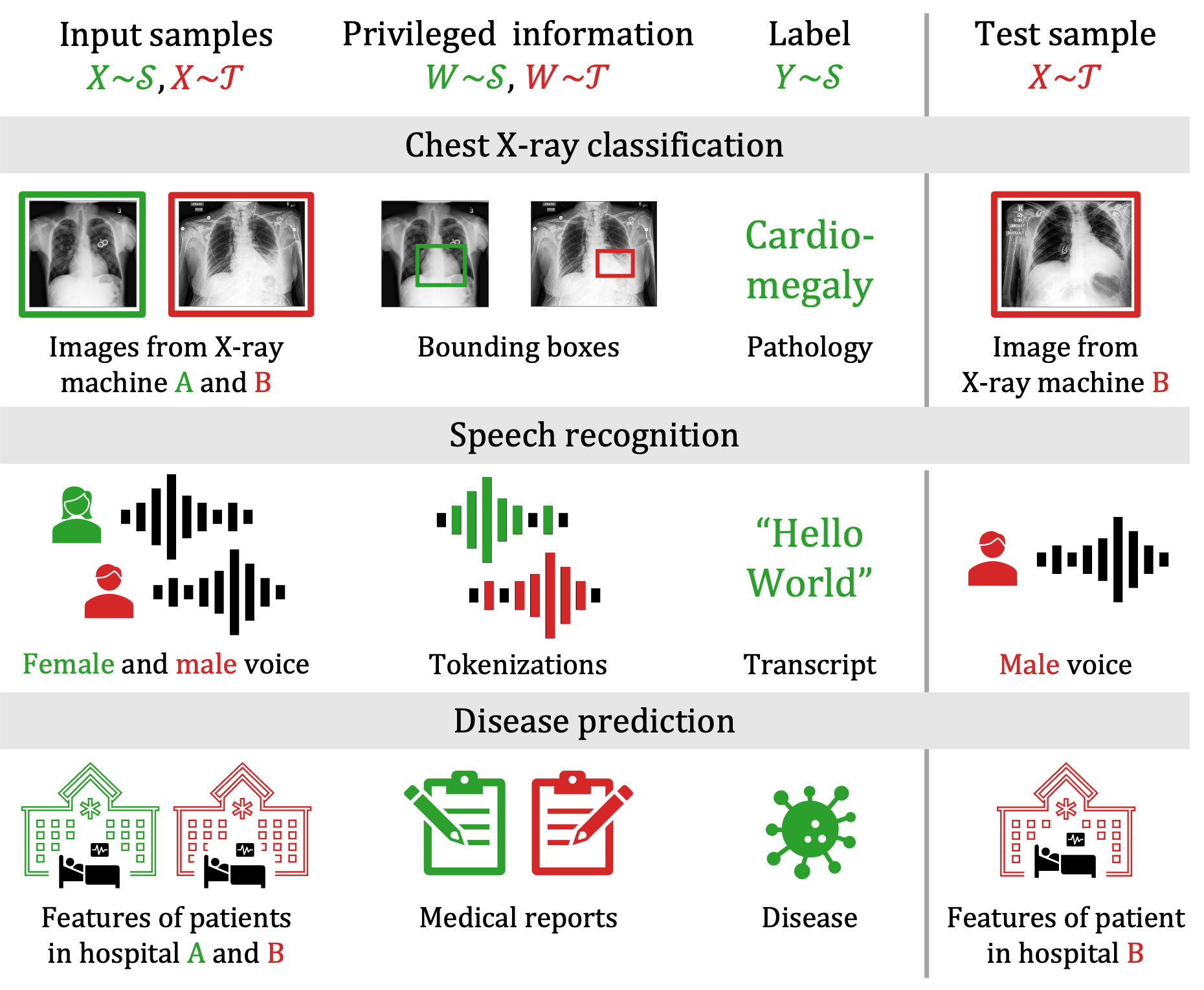
Figure 1: Examples of domain adaptation by learning using privileged information (DALUPI). During training, input samples $X$ and privileged information $W$ are available from both source and target domains. Labels $Y$ are only available for inputs from the source domain. At test time, a target sample $X$ is observed. Top: Chest X-ray images $X$ together with pathology masks $W$ and diagnosis label $Y$. Middle: Tokenizations $W$ accompany recorded speech $X$ during learning of a speech recognition system. Bottom: Clinical notes $W$ add information to a system learning to predict disease progression from patient features $X$.

It is well-known that privileged information can be used to improve sample efficiency (reduce variance) in learning (Vapnik & Izmailov, 2015; Pechyony & Vapnik, 2010; Jung & Johansson, 2022). Next, we will show that privileged information can provide identifiability of the target risk—that it may be computed from the observational distribution—even when overlap is not satisfied in the input variable $X$.

To identify $R_{\mathcal{T}}$ (1) without overlap in $X$, we require the additional assumption that $W$ is sufficient for $Y$ given $X$.

Assumption 3 (Sufficiency of privileged information).

Privileged information $W$ is sufficient for the outcome $Y$ given covariates $X$ if $Y\perp X\mid W$ in both $\mathcal{S}$ and $\mathcal{T}$.

Assumption 3 is satisfied when $X$ provides no more information about $Y$ in the presence of $W$. In our running example, if $W$ is the subset of X-ray pixels corresponding to an area indicating a medical problem, the other pixels in $X$ may be unnecessary to make a good prediction of $Y$. Moreover, if covariate shift and overlap are satisfied w.r.t. $W$, i.e., there is some probability of observing the restricted pixel subset in both domains, we have the following proposition.

Proposition 1.

Let Assumptions 1 and 2 be satisfied w.r.t. $W$ (not necessarily w.r.t. $X$) and let Assumption 3 hold as stated. Then, the target risk $R_{\mathcal{T}}$ is identified and

$$R_{\mathcal{T}}(h) =\sum_{x}\mathcal{T}(x)\sum_{w}\mathcal{T}(w\mid x)\sum_{y}\mathcal{S}(y\mid w)L(h(x),y)~{}.$$

Proof.

By definition, $R_{\mathcal{T}}(h)=\sum_{x,y}\mathcal{T}(x,y)L(h(x),y)$. We then marginalize over privileged information $W$,

$$\mathcal{T}(y\mid x) =\mathbb{E}_{\mathcal{T}(W\mid x)}[\mathcal{T}(y\mid W)\mid x]$$

$$=\sum_{w:\mathcal{S}(w)>0}\mathcal{T}(w\mid x)\mathcal{S}(y\mid w)~{},$$

where the first equality follows by sufficiency and the second by covariate shift and overlap in $W$. $\mathcal{T}(x),\mathcal{T}(w\mid x)$ and $\mathcal{S}(y\mid w)$ are observable through training samples. ∎

Proposition 1 allows us to relax the standard assumption of overlap in $X$ at the cost of collecting additional variables. When $W$ is a subset of the information in $X$, as in our running example, overlap in $X$ implies overlap in $W$, but not vice versa. Moreover, under Assumption 3, if covariate shift holds for $X$, it holds also for $W$.

Proposition 1 shows that there are conditions where privileged information allows for identification of a target-optimal hypothesis where identification is not possible without it, e.g., when overlap is violated in $X$ (Johansson et al., 2019). Intuitively, $W$ guides the learner toward the information in $X$ which is relevant for the label. The conditions on $W$ may be compared to the properties of the representation mapping in Construction 4.1 of (Wu et al., 2019). Finally, we note that Proposition 1 does not require that $X$ is ever observed in the source domain $\mathcal{S}$.

3.1 A simple two-stage algorithm and its risk

Under Assumption 3, a natural strategy for predicting the outcome $Y$ is to first infer the privileged information $W$ from $X$ using a function $\hat{f}$, and then predict $Y$ using a function $\hat{g}$ applied to the inferred value, $\hat{h}=\hat{g}(\hat{f}(X))$. We may find such functions $\hat{f}$, $\hat{g}$ by solving two separate empirical risk minimization (ERM) problems, as follows.

$$\hat{f} \coloneqq\operatorname*{arg\,min}_{f\in\mathcal{F}}\hat{R}^{W}_{\mathcal{T}}(f),\hat{R}^{W}_{\mathcal{T}}(f)=\frac{1}{n}\sum_{i=1}^{n}L(f(\tilde{x}_{i}),\tilde{w}_{i})$$ (2)

$$\hat{g} \coloneqq\operatorname*{arg\,min}_{g\in\mathcal{G}}\hat{R}^{Y}_{\mathcal{S}}(g),\;\hat{R}^{Y}_{\mathcal{S}}(g)=\frac{1}{m}\sum_{i=1}^{m}L(g(w_{i}),y_{i})$$

Hypothesis classes $\mathcal{F},\mathcal{G}$ may be chosen so that the class $\mathcal{H}=\{h=g\circ f;(f,g)\in\mathcal{F}\times\mathcal{G}\}$ has a desired form. We can bound the generalization error of an estimator $\hat{h}=\hat{g}\circ\hat{f}$ of the form above, when $W\in\mathbb{R}^{d_{\mathcal{W}}}$ and $L$ is the squared loss, by placing a Lipschitz assumption on the space of prediction functions $\mathcal{G}$, i.e., $\forall g\in\mathcal{G},w,w^{\prime}\in\mathcal{W},~{}\|g(w)-g(w^{\prime})\|_{2}\leq M\|w-w^{\prime}\|_{2}$. For this, we first define the $\rho$-weighted prediction risk in the source domain,

$$R^{Y,\rho}_{\mathcal{S}}(g)=\mathbb{E}_{\mathcal{S}(W,Y)}[\rho(W)L(g(W),Y)]$$

where $\rho$ is the density ratio of $\mathcal{T}$ and $\mathcal{S}$, $\rho(w)=\frac{\mathcal{T}(w)}{\mathcal{S}(w)}$. We define the empirical weighted risk $\hat{R}^{Y,\rho}_{S}(g)$ analogously to the above. When the density ratio $\rho$ is not known one might use density estimation (Sugiyama et al., 2012) or probabilistic classifiers to estimate it. We now have the following result which we prove for univariate $Y$; the result can be generalized to multiple classes with standard methods.

Proposition 2.

Assume that $\mathcal{G}$ comprises M-Lipschitz mappings from the privileged information space $\mathcal{W}\subseteq\mathbb{R}^{d_{W}}$ to $\mathcal{Y}$. Further, assume that both the ground truth privileged information $W$ and label $Y$ are deterministic in $X$ and $W$, respectively. Let $\rho$ be the domain density ratio of $W$ and let Assumptions 1–3 (Covariate shift, Overlap and Sufficiency) hold with respect to $W$. Further, let $L$ be the squared Euclidean distance and assume that $L(\hat{f}(w),Y)$ is uniformly bounded over $\mathcal{W}$ by a constant $B$ and let $d$ and $d^{\prime}$ be the pseudo-dimensions of $\mathcal{G}$ and $\mathcal{F}$, respectively. Assume that there are $n$ observations each from the source (labeled) and target (unlabeled) domains. Then, for any $h=f\circ g\in\mathcal{F}\times\mathcal{G}$, with probability at least $1-\delta$,

$$\frac{R_{\mathcal{T}}(h)}{2} \leq\hat{R}^{Y,\rho}_{\mathcal{S}}(g)+M^{2}\hat{R}^{W}_{\mathcal{T}}(f)$$

$$+\mathcal{O}\left(\sqrt[3/8]{\frac{d\log\frac{n}{d}}{n}}+\sqrt{\frac{d^{\prime}\log\frac{n}{d^{\prime}}}{n}}\right)~{}.$$

Proof sketch.

Decomposing the risk of $h\circ\phi$ , we get

$$R_{\mathcal{T}}(h)=\mathbb{E}_{\mathcal{T}}[(g(f(X))-Y)^{2}]$$

$$\leq 2\mathbb{E}_{\mathcal{T}}[(g(W)-Y)^{2}]+2M^{2}\mathbb{E}_{\mathcal{T}}[\|(f(X)-W)\|^{2}]$$

$$=2R^{Y}_{\mathcal{T}}(g)+2M^{2}R^{W}_{\mathcal{T}}(f)=2R^{Y,\rho}_{S}(g)+2M^{2}R^{W}_{\mathcal{T}}(f)~{}.$$

The first inequality follows the relaxed triangle inequality and the Lipschitz property, and the third equality from Overlap and Covariate shift. Treating each component of $\hat{w}$ as independent, using standard PAC learning results, and application of Theorem 3 from Cortes et al. (2010) along with a union bound argument, we get the stated result. See Appendix C for a more detailed proof. ∎

As a result of Proposition 2, when $\mathcal{F}$ and $\mathcal{G}$ contain the ground-truth mappings between $X$ and $W$ and between $W$ and $Y$, in the limit of infinite samples, minimizers of (2) minimize $R_{\mathcal{T}}$ as well.

4 Image classification under domain shift with privileged information

Image classification remains one of the primary benchmark tasks for unsupervised domain adaptation. In our experiments, we consider multi-class and multi-label image classification tasks where privileged information $W$ highlights regions of interest in the images, related to the labels $Y$. Specifically, $W$ is the pixels contained within one or more bounding boxes, represented by pixel coordinates $T\in\mathbb{R}^{4}$.

In the multi-class case, each image has a single bounding box whose corresponding pixels determine a single label $Y$ of the image. In the multi-label case, an observation $(x_{i},w_{i},y_{i})$ may contain multiple bounding boxes $j\in\{1,\ldots,J\}$, with coordinates $t_{ij}$, each of which is assigned a multi-class label $u_{ij}$. The image label $y_{i}$ constitutes the set of observed bounding box labels in the image. Next, we propose algorithms that leverage privileged information for improved domain transfer in these two tasks.

4.1 DALUPI-TS: A two-stage algorithm for multi-class image classification

Our first algorithm, which we call DALUPI-TS, conforms to our theoretical analysis and instantiates (2) for the multi-class image classification problem by separately fitting functions $\hat{f}\in\mathcal{F}$ and $\hat{g}\in\mathcal{G}$ to infer privileged information $W$ and predict $Y$. $\hat{f}$ takes an input image $X$ and (i) estimates the location of a single bounding box, (ii) cuts out the corresponding part of the image $X$, and (iii) resizes it to a set dimension. Steps (ii)–(iii) are hard coded (not learned). The pixels $W$ defining a region of interest are fed to $\hat{g}$ which outputs a prediction of the image label $Y$.

In experiments, we use convolutional neural networks for both $\hat{f}$ and $\hat{g}$. The two estimators are trained separately on $(\tilde{x},\tilde{w})\sim\mathcal{T}$ and $(w,y)\sim\mathcal{S}$, respectively, as in (2), and then evaluated on target domain images where the output of $\hat{f}$ is used for prediction with $\hat{g}$. We use the mean squared error loss for $\hat{f}$ and categorical cross-entropy loss for $\hat{g}$.

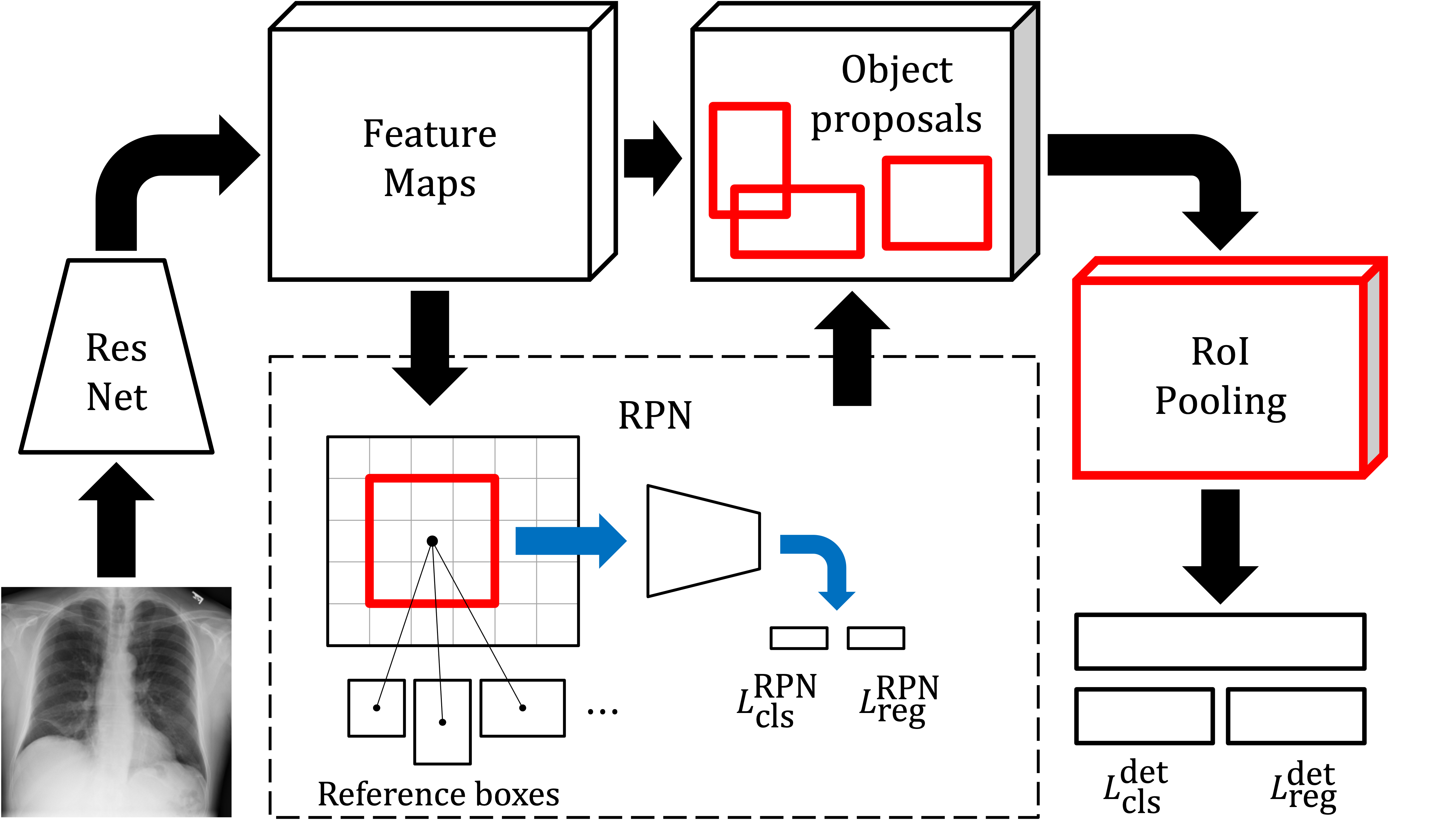
Figure 2: Faster R-CNN Ren et al. (2016). The RoI pooling layer and the classification and regression layers are part of the Fast R-CNN detection network Girshick (2015).

4.2 DALUPI-E2E: An end-to-end solution for multi-label image classification

For multi-label classification, we adapt Faster R-CNN (Ren et al., 2016) outlined in Figure 2 and described below. Faster R-CNN uses a region proposal network (RPN) to generate region proposals which are fed to a detection network for classification and bounding box regression. This way of solving the task in subsequent steps has similarities with our two-stage algorithm although Faster R-CNN can be trained end-to-end. We make small modifications to the training procedure of the original model in the end of this section.

The RPN generates region proposals relative to a fixed number of reference boxes—anchors—centered at the locations of a sliding window moving over convolutional feature maps. Each anchor is assigned a binary label $p\in\{0,1\}$ based on its overlap with ground-truth bounding boxes; positive anchors are also associated with a ground-truth box with location $t$. The RPN loss for a single anchor is

$$L^{\text{RPN}}(\hat{p},p,\hat{t},t):=L_{\text{cls}}^{\text{RPN}}(\hat{p},p)+pL_{\text{reg}}^{\text{RPN}}(\hat{t},t),$$ (3)

where $\hat{t}$ represents the refined location of the anchor and $\hat{p}$ is the estimated probability that the anchor contains an object. The binary cross-entropy loss and a smooth $L_{1}$ loss are used for the classification loss $L^{\text{RPN}}_{\text{cls}}$ and the regression loss $L^{\text{RPN}}_{\text{reg}}$, respectively. For a mini-batch of images, the total RPN loss is computed based on a subset of all anchors, sampled to have a ratio of up to 1:1 between positive and negative ditto.

A filtered set of region proposals are projected onto the convolutional feature maps. For each proposal, the detection network—Fast R-CNN Girshick (2015)—outputs a probability $\hat{p}(k)$ and a predicted bounding box location $\hat{t}(k)$ for each class $k$. Let $\hat{p}=(\hat{p}(0),\ldots,\hat{p}(K))$, where $\sum_{k}\hat{p}(k)=1$, $K$ is the number of classes and $0$ represents a catch-all background class. For a single proposal with ground-truth coordinates $t$ and multi-class label $u\in\{0,\ldots,K\}$, the detection loss is

$$L^{\text{det}}(\hat{p},u,\hat{t}_{u},t)=L_{\text{cls}}^{\text{det}}(\hat{p},u)+\mathbf{I}_{u\geq 1}L_{\text{reg}}^{\text{det}}(\hat{t}_{u},t),$$ (4)

where $L_{\text{cls}}^{\text{det}}(\hat{p},u)=-\log{\hat{p}(u)}$ and $L_{\text{reg}}^{\text{det}}$ is a smooth $L_{1}$ loss. To obtain a probability vector for the entire image, we maximize, for each class $k$, over the probabilities of all proposals.

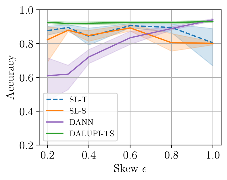
(a) Source test accuracy.

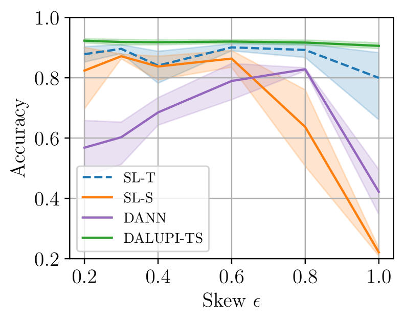
(b) Target test accuracy.

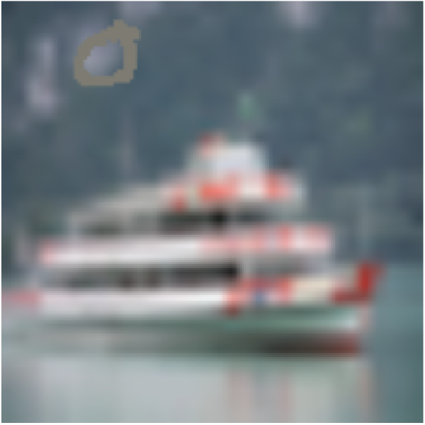
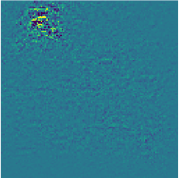
(c) SL-S, $\epsilon=0.2$.

(d) SL-S, $\epsilon=1.0$.

Figure 3: Digit classificastion task. Model performance on source (a) and target (b) domains as a function of association $\epsilon$ between background and label in $\mathcal{S}$. As the skew increases, the performance of the source models on the target data deteriorates. The rightmost panels show two example images (top) from the dataset as well as saliency maps (bottom) from SL-S when trained with source domain skew $\epsilon=0.2$ (c) and $\epsilon=1$ (d).

During training, Faster R-CNN requires that all input images $x$ come with at least one ground-truth annotation (bounding box) $w$ and its corresponding label $u$. To increase sample-efficiency, we enable training the model using non-annotated but labeled samples $(x,y)$ from the source domain and annotated but unlabeled samples $(\tilde{x},\tilde{w})$ from the target domain. In the RPN, no labels are needed, and we simply ignore anchors from non-annotated images when sampling anchors for the loss computation. For the computation of (4), we handle the two cases separately. We assign the label $u=-1$ to all ground-truth annotations from the target domain and multiply $L_{\text{cls}}^{\text{det}}$ by the indicator $\mathbf{I}_{u\geq 0}$. For non-annotated samples $(x,y)$ from the source domain, there are no box-specific coordinates $t$ or labels $u$ but only the labels $y$ for the entire image. In this case, (4) is undefined and we instead compute the binary cross-entropy loss between binarized labels and the probability vector for the entire image.

We train the RPN and the detection network jointly as described in Ren et al. (2016). To extract feature maps, we use a Feature Pyramid Network Lin et al. (2017) on top of a ResNet-50 architecture He et al. (2016). We use the modfied model—DALUPI-E2E—in the experiments in Section 5.2 and 5.3. Note that we may also train the model in a LUPI setting, where no information from the target domain is used, in which case we call it LUPI-E2E.

5 Experiments

We compare our models, DALUPI-TS and DALUPI-E2E, to baseline algorithms in three image classification tasks where privileged information is available as one or more bounding boxes highlighting regions of interest related to the image label. We use DALUPI-TS in a digit classification task in Section 5.1. DALUPI-E2E is then used in the experiments in Section 5.2 and 5.3, where we consider classification of entities from the MS-COCO dataset and pathologies in chest X-ray images. LUPI-E2E is included in the entity classification task.

As baselines, we use classifiers trained on labeled examples from the source and target domain, respectively. The latter serves as an oracle comparison since labels are unavailable from the target in our setting. Both models are ResNet-based convolutional neural networks adapted for the different experiments and we refer to them as SL-S and SL-T, respectively. We also compare our models to a domain-adversarial neural network (DANN) Ganin et al. (2016) trained on labeled data from the source domain and unlabeled data from the target domain.

For each experiment setting (task, skew, amount of privileged information, etc.), we train 10 models from each relevant model class using randomly selected hyperparameters. All models are evaluated on a hold-out validation set from the source domain and the best performing model in each class is then evaluated on hold-out test sets from both domains. For SL-T, we use a hold-out validation set from the target domain. We repeat this procedure over 5–10 seeds controlling the data splits and the random number generation in PyTorch, which is used in our implementation. We report $95\text{\,}\mathrm{\char 37\relax}$ confidence intervals computed by bootstrapping over the seeds. We refer to Appendix A for further details on experiments.

5.1 Digit classification

We construct a synthetic image dataset, based on the assumptions of Proposition 1, to verify that there are problems where domain adaptation using privileged information is guaranteed successful transfer but standard UDA is not.
We start with images from CIFAR-10 (Krizhevsky, 2009) which have been upscaled to $128\times 128$. Then we insert a random $28\times 28$ digit image, with a label in the range 0–4, from the MNIST dataset (Lecun, 1998) into a random location of the CIFAR-10 image, forming the input image $X$ (see Figures 3(c)–3(d) for examples). The label $Y\in\{0,\dots,4\}$ is determined by the MNIST digit. We store the bounding box around the inserted digit image and use the pixels contained within it as privileged information $W$. This is done until no more digit images remain. The domains are constructed from using CIFAR-10’s first five and last five classes as source and target backgrounds, respectively. Both source and target datasets contain $15\,298\text{\,}\mathrm{i}$mages each.

To increase the difficulty of the task, we make the digit be the mean colour of the dataset and make the digit background transparent so that the border of the image is less distinct. This may slightly violate Assumption 2 w.r.t. $W$ since the backgrounds differ between domains. To understand how successful transfer depends on domain overlap and access to sufficient privileged information, we include a skew parameter $\epsilon\in[\frac{1}{c},1]$, where $c=5$ is the number of digit classes, which determines the correlation between digits and backgrounds. For a source image $i$ with digit label $Y_{i}\in\{0,...,4\}$, we select a random CIFAR-10 image with class $B_{i}\in\{0,\dots,4\}$ with probability

$$P(B_{i}=b\mid Y_{i}=y)=\left\{\begin{array}[]{ll}\epsilon,&\mbox{if}\;b=y\\ (1-\epsilon)/(c-1),&\mbox{otherwise}\end{array}\right..$$

For target images, digits and backgrounds are matched uniformly at random. Note that the choice of $\epsilon=\frac{1}{c}$ yields a uniform distribution and $\epsilon=1$ being equivalent to the background carrying as much signal as the privileged information. We hypothesise that the latter part would be the worst possible case where confusion of the model is likely, which would lead to poor generalization performance.

In Figure 3(b), we can indeed observe the conjectured behavior where, as the skew $\epsilon$ increases, the performance of SL-S decreases substantially on the target domain. Thus an association with the background might harm generalization performance which has been observed in previous work where background artifacts in X-ray images confused the resulting classifier.

We can also observe that DANN does not seem to be robust to the increase in correlation between the label and the background. In contrast, DALUPI-TS is unaffected by the increased skew as the subset of pixels only carries some of the background information with it, while containing sufficient information to make good predictions. Interestingly, DALUPI-TS also seems to be as good or slightly better than the oracle SL-T in this setting. This may be due to improved sample efficiency from using PI.

5.2 Entity classification

We evaluate DALUPI-E2E and LUPI-E2E on an entity classification task based on images from the MS-COCO dataset (Lin et al., 2014). We define the source and target domains as indoor and outdoor images, respectively, and consider four entity classes for the label $Y$: person, cat, dog, and bird. We extract indoor images by filtering out images from the super categories “indoor” and “appliance” that also contain at least one of the entity classes. Outdoor images are extracted in the same way using the super categories “vehicle” and “outdoor”. Images that for some reason occur in both domains (for example an indoor image with a toy car) are removed along with any gray-scale images. We also include 1000 background examples, i.e., images with none of the entities present, in both domains.

In total, there are $5231\text{\,}\mathrm{i}$mages in the source domain and $5719\text{\,}\mathrm{i}$mages in the target domain; the distribution of labels are provided in Appendix A. From these pools we randomly sample $3000\text{\,}\mathrm{,}$ $1000\text{\,}\mathrm{,}$ and $1000\text{\,}\mathrm{i}$mages for training, validation, and testing, respectively. As privileged information $W$, we use bounding boxes localizing the different entities. We assume that the assumptions of Proposition 1 hold. In particular, it is reasonable to assume that the pixels contained in a box are sufficient for classifying the object.

The purpose of this experiment is to investigate the effect of additional privileged information (PI). We give LUPI-E2E access to all $(x,y)$ samples from the source domain and increase the fraction of inputs for which PI is available, $n_{\text{PI}}(\mathcal{S})$, from 0 to 1. For DALUPI-E2E, we increase the fraction of $(\tilde{x},\tilde{w})$ samples from the target domain, $n_{\text{PI}}(\mathcal{T})$, from 0 to 1, while keeping $n_{\text{PI}}(\mathcal{S})=1$. We train SL-S and SL-T using all available data and increase the fraction of unlabeled target samples DANN sees from 0.2 to 1.

The models’ test AUC, averaged over the four entity classes, in the target domain is shown in Figure 4. The performance of LUPI-E2E increases as $n_{\text{PI}}(\mathcal{S})$ increases, but even with access to all PI in the source domain, LUPI-E2E barely beats SL-S. However, when additional $(\tilde{x},\tilde{w})$ samples from the target domain are added, DALUPI-E2E quickly outperforms SL-S and eventually reaches the performance of SL-T. We note that DANN does not benefit as much from the added unlabeled target samples as DALUPI-E2E does. The large gap between LUPI-E2E and SL-S for $n_{\text{PI}}(\mathcal{S})=0$ is not too surprising; we do not expect an object detector to work well without bounding box supervision.

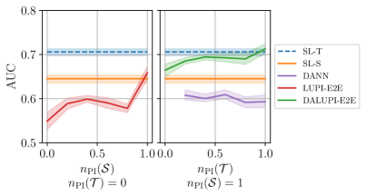
Figure 4: Model performance in the target domain for the entity classification task. The point performance of SL-S and SL-T is extended across the x-axes for visual purposes. DANN is trained with an increasing fraction of target samples $\tilde{x}$ but uses no PI.

5.3 X-ray classification

As a real-world experiment, we study detection of pathologies in chest X-ray images. We use the ChestX-ray8 dataset Wang et al. (2017) as source domain and the CheXpert dataset Irvin et al. (2019) as target domain. As privileged information, we use bounding boxes localizing each pathology. For the CheXpert dataset, only pixel-level segmentations of pathologies are available, and we create bounding boxes that tightly enclose the segmentations. It is not obvious that the pixels within such a bounding box are sufficient for classifying the pathology, and we suspect that we may violate the assumptions of Proposition 1 in this experiment. However, as we find below, DALUPI-E2E improves empirical performance compared to baselines for small training sets, thereby demonstrating increased sample efficiency.

We consider the three pathologies that exist in both datasets and for which there are annotated findings: atelectasis (ATL; collapsed lung), cardiomegaly (CM; enlarged heart), and pleural effusion (PE; water around the lung). There are 457 and 118 annotated images in the source and target domain, respectively. We train DALUPI-E2E and DANN using all these images. SL-S is trained with the 457 source images and SL-T with the 118 target images as well as 339 labeled but non-annotated target images. Neither SL-S, SL-T nor DANN use any privileged information. In the annotated images, there are 180/146/153 and 75/66/64 examples of ATL/CM/PE in each domain respectively. Validation and test sets are sampled from the non-annotated images.

In Table 2 we present the per-class AUCs in the target domain. DALUPI-E2E outperforms all baseline models, including the target oracle, in detecting CM. For ATL and PE, it performs similarly to the other feasible models. That SL-T is better at predicting PE is not surprising given that this pathology is most prevalent in the target domain. In Figure 5(a), we show a single-finding image from the target test set with ground-truth label CM. The predicted bounding box of DALUPI-E2E with the highest probability is added to the image. DALUPI-E2E identifies the region of interest and makes a correct classification. The bottom panel shows the saliency map for the ground truth class for SL-S. We see that the gradients are mostly constant, indicating that the model is uncertain. In Figure 5(b), we show AUC for CM for DALUPI-E2E, SL-S, and SL-T trained with additional examples without bounding box annotations. We see that SL-S catches up to the performance of DALUPI-E2E when a large amount of labeled examples are provided. These results indicate that identifiability is not the primary obstacle for adaptation, and that PI improves sample efficiency.

Table 2: X-ray task. Test AUC for the three pathologies in the target domain for all considered models. Boldface indicates the best-performing feasible model; SL-T uses target labels.

	ATL	CM	PE
SL-T	57 (56, 58)	59 (55, 63)	79 (78, 80)
SL-S	55 (55, 56)	61 (58, 64)	73 (70, 75)
DANN	56 (54, 57)	61 (56, 66)	73 (71, 75)
DALUPI-E2E	55 (55, 56)	72 (71, 73)	74 (72, 76)

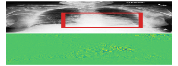
(a) DALUPI-E2E vs SL-S.

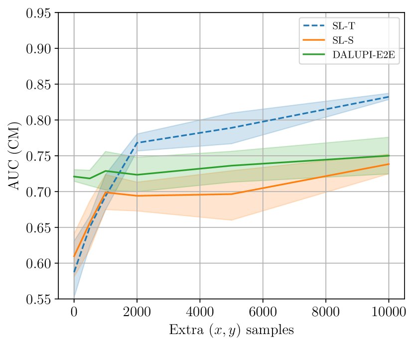
(b) Test AUC for CM in $\mathcal{T}$.

Figure 5: X-ray task. (a): An example image from the target test set with label CM. The red rectangle indicates the bounding box with the highest probability as predicted by DALUPI-E2E with no extra data. The saliency map for CM for the corresponding SL-S is shown below. (b): AUC for CM in the target test set for SL-S, SL-T, and DALUPI-E2E trained with additional $(x,y)$ samples.

6 Related work

Learning using privileged information (LUPI) was first introduced by Vapnik & Vashist (2009) for support vector machines (SVMs), and was later extended to empirical risk minimization (Pechyony & Vapnik, 2010). Methods using PI, which is sometimes called hidden information or side information, has since been applied in many diverse settings such as healthcare (Shaikh et al., 2020), finance (Silva et al., 2010), clustering (Feyereisl & Aickelin, 2012) and image recognition (Vu et al., 2019; Hoffman et al., 2016). Related concepts include knowledge distillation (Hinton et al., 2015; Lopez-Paz et al., 2016), where a teacher model trained on additional variables adds supervision to a student model, and weak supervision (Robinson et al., 2020) where so-called weak labels are used to learn embeddings, subsequently used for the task of interest. The use of PI for deep image classification has been investigated by Chen et al. (2017) but this only covered regular supervised learning. Finally, Sharmanska et al. (2014) used regions of interest in images as privileged information to improve the accuracy of image classifiers, but did not consider domain shift.

Domain adaptation using PI has been considered before with SVMs (Li et al., 2022; Sarafianos et al., 2017). Vu et al. (2019) used scene depth as PI in semantic segmentation using deep neural networks. However, they only use PI from the source domain and they do not provide any theoretical analysis. Motiian (2019) investigate PI and domain adaptation using the information bottleneck method for visual recognition. However, their setting differs from ours in that each observation comprises source-domain and target domain features, a label and PI.

7 Discussion

We have presented our framework DALUPI which leverages privileged information for unsupervised domain adaptation. The framework builds on an alternative set of assumptions which can more realistically be satisfied in high-dimensional problems than classical assumptions of covariate shift and domain overlap, at the cost of collecting a larger variable set for training. Our analysis of this setting inspired practical algorithms for multi-class and multi-label image classification.

Our experiments show tasks where domain adaptation using privileged information is successful while regular adaptation methods fail, in particular when the assumptions of our analysis are satisfied. We observe empirically also that methods using privileged information are more sample-efficient than comparable non-privileged learners, in line with the literature. In fact, DALUPI models occasionally even outperform oracle models trained using target labels due to their sample efficiency. Thus, we recommend considering these methods in small-sample settings.

To avoid assuming that domain overlap is satisfied with respect to input covariates, we require that privileged information is sufficient to determine the label. This can be limiting in problems where sufficiency is difficult to verify. However, in our motivating example of image classification, a domain expert could deliberately choose PI so that sufficiency is reasonably satisfied. In future work, the framework might be applied to a more diverse set of tasks, with different modalities to investigate if the findings here can be replicated. Using PI may be viewed as “building in” domain-knowledge in the structure of the adaptation problem and we see this as promising approach for further UDA research.

Appendix A Experimental details

In this section give further details of the experiments. All code is written in Python and we use PyTorch in combination with skorch Tietz et al. (2017) for our implementations of the networks. For Faster R-CNN, we adapt the implementation provided by torchvision through the function fasterrcnn_resnet50_fpn. DANN is implemented with different optimizers for the discriminator and the generator. Here, the generator is the main network consisting of a ResNet-based encoder and a classifier network. We set the parameter $\lambda$, which controls the amount of domain adaption regularization, to a fixed value 0.1 in all experiments. We add a gradient penalty to the discriminator loss which we control with the parameter “gradient penalty” specified in each experiment. We also include a parameter controlling the number of discriminator steps per generator steps (default 1). The source and target baselines are based on the ResNet-50 architecture if nothing else is stated. All models are trained using NVIDIA Tesla A40 GPUs. In experiment, we use the Adam optimizer. The code will be made available.

A.1 Digit classification

We use $20\text{\,}\mathrm{\char 37\relax}$ of the available source and target data in the test set. We likewise use $20\text{\,}\mathrm{\char 37\relax}$ of the training data for validation purposes. For the baselines SL-S and SL-T we use a ResNet-18 network without pretrained weights. We change the final fully connected layer from stock to the following sequence:

• fully connected layer with 256 neurons

• batch normalization layer

• dropout layer with $p=0.2$

• fully connected layer with 128 neurons

• fully connected layer with 5 neurons.

For DALUPI-TS we use a non-pretrained ResNet-18 for the $\hat{f}$ function where we replace the default fully connected layer with a fully connected layer with 4 neurons to predict the coordinates of the bounding box. The predicted bounding box is resized to a $28\times 28$ square no matter the initial size. We use a simpler convolutional neural network for the $\hat{g}$ function with the structure as follows:

• convolutional layer with 16 out channels, kernel size of 5, stride of 1, and padding of 2

• max pooling layer with kernel size 2, followed by a ReLU activation

• convolutional layer with 32 out channels, kernel size of 5, stride of 1, and padding of 2

• max pooling layer with kernel size 2, followed by a ReLU activation

• dropout layer with $p=0.4$

• fully connected layer with 50 neurons

• dropout layer with $p=0.2$

• fully connected layer with 5 neurons.

The training is stopped when the best validation error does not improve over 5 epochs or when 100 epochs have been trained, whichever occurs first. The training of the DANN model is stopped when the validation loss has not improved over 10 epochs. DANN is pretrained on ImageNet.

A.1.1 Hyperparameters

We randomly choose hyperparameters from the following predefined sets of values:

• SL-S and SL-T:

  • batch size: $(16,32,64)$

  • learning rate: ($1.0\text{\times}{10}^{-04}\text{\,}\mathrm{,}$ $5.0\text{\times}{10}^{-04}\text{\,}\mathrm{,}$ $1.0\text{\times}{10}^{-03}\text{\,}\mathrm{)}$

  • weight decay: ($1.0\text{\times}{10}^{-06}\text{\,}\mathrm{,}$ $1.0\text{\times}{10}^{-05}\text{\,}\mathrm{,}$ $1.0\text{\times}{10}^{-04}\text{\,}\mathrm{,}$ $1.0\text{\times}{10}^{-03}\text{\,}\mathrm{)}$.

• DALUPI-TS

  • batch size: $(16,32,64)$

  • learning rate: ($1.0\text{\times}{10}^{-04}\text{\,}\mathrm{,}$ $5.0\text{\times}{10}^{-04}\text{\,}\mathrm{,}$ $1.0\text{\times}{10}^{-03}\text{\,}\mathrm{)}$.

• DANN

  • batch size: $(64)$

  • learning rate: ($1.0\text{\times}{10}^{-03}\text{\,}\mathrm{)}$

  • gradient penalty: $(0,0.01,0.1)$

  • weight decay: ($1.0\text{\times}{10}^{-04}\text{\,}\mathrm{,}$ $1.0\text{\times}{10}^{-03}\text{\,}\mathrm{)}$

  • number of trainable layers (encoder): $(1,2,3)$

  • dropout (encoder): $(0,0.1,0.2,0.5)$

  • width of discriminator network: $(64,128,256)$

  • depth of discriminator network: $(2,3)$.

A.2 Entity classification

In the entity classification experiment, we train all models for at most 50 epochs. If the validation AUC does not improve for 10 subsequent epochs, we stop the training earlier. No pretrained weights are used in this experiment since we find that the task is too easy to solve with pretrained weights. For DALUPI-E2E and LUPI-E2E we use the default anchor sizes for each of the feature maps (32, 64, 128, 256, 512), and for each anchor size we use the default aspect ratios (0.5, 1.0, 2.0). We use the binary cross entropy loss for SL-S, SL-T, and DANN.

We use the 2017 version of the MS-COCO dataset Lin et al. (2014). In Table 3 we describe the label distribution in the defined source and target domains, respectively. How the domains are defined are described in Section 5.2.

Table 3: Marginal label distribution in source and target domains for the entity classification task based on the MS-COCO dataset. The background class contains images where none of the four entities are present.

Domain	Person	Dog	Cat	Bird	Background
Source	2963	569	1008	213	1000
Target	3631	1121	423	712	1000

A.2.1 Hyperparameters

We randomly choose hyperparameters from the following predefined sets of values. For information about the specific parameters in LUPI-E2E and DALUPI-E2E, we refer to the paper by Ren et al. (2016). RoI and NMS refer to region of interest and non-maximum suppression, respectively.

• SL-S and SL-T:

  • batch size: $(16,32,64)$

  • learning rate: ($1.0\text{\times}{10}^{-04}\text{\,}\mathrm{,}$ $5.0\text{\times}{10}^{-04}\text{\,}\mathrm{,}$ $1.0\text{\times}{10}^{-03}\text{\,}\mathrm{)}$

  • weight decay: ($1.0\text{\times}{10}^{-4}\text{\,}\mathrm{,}$ $1.0\text{\times}{10}^{-3}\text{\,}\mathrm{)}$

  • nonlinear classifier: (True, False)

  • dropout (encoder): (0, 0.1, 0.2, 0.3).

• DANN:

  • batch size: $(16,32,64)$

  • learning rate: ($1.0\text{\times}{10}^{-04}\text{\,}\mathrm{,}$ $5.0\text{\times}{10}^{-04}\text{\,}\mathrm{,}$ $1.0\text{\times}{10}^{-03}\text{\,}\mathrm{)}$

  • discriminator updates per generator updates: (1, 2)

  • gradient penalty: (0, 0.01, 0.1)

  • weight decay (generator): ($1.0\text{\times}{10}^{-4}\text{\,}\mathrm{,}$ $1.0\text{\times}{10}^{-3}\text{\,}\mathrm{)}$

  • weight decay (discriminator): ($1.0\text{\times}{10}^{-4}\text{\,}\mathrm{,}$ $1.0\text{\times}{10}^{-3}\text{\,}\mathrm{)}$

  • number of trainable layers (encoder): (1, 2, 3, 4, 5)

  • dropout (encoder): (0, 0.1, 0.2, 0.3)

  • width of discriminator network: (64, 128, 256)

  • depth of discriminator network: (2, 3)

  • nonlinear classifier: (True, False).

• LUPI-E2E and DALUPI-E2E:

  • batch size: $(16,32,64)$

  • learning rate: ($1.0\text{\times}{10}^{-04}\text{\,}\mathrm{,}$ $1.0\text{\times}{10}^{-03}\text{\,}\mathrm{)}$

  • weight decay: ($1.0\text{\times}{10}^{-4}\text{\,}\mathrm{,}$ $1.0\text{\times}{10}^{-3}\text{\,}\mathrm{)}$

  • IoU foreground threshold (RPN): (0.6, 0.7, 0.8, 0.9)

  • IoU background threshold (RPN): (0.2, 0.3, 0.4)

  • batchsize per image (RPN): (32, 64, 128, 256)

  • fraction of positive samples (RPN): (0.4, 0.5, 0.6, 0.7)

  • NMS threshold (RPN): (0.6, 0.7, 0.8)

  • RoI pooling output size (Fast R-CNN): (5, 7, 9)

  • IoU foreground threshold (Fast R-CNN): (0.5, 0.6)

  • IoU background threshold (Fast R-CNN): (0.4, 0.5)

  • batchsize per image (Fast R-CNN): (16, 32, 64, 128)

  • fraction of positive samples (Fast R-CNN: (0.2, 0.25, 0.3)

  • NMS threshold (Fast R-CNN): (0.4, 0.5, 0.6)

  • detections per image (Fast R-CNN): (25, 50, 75, 100).

A.3 X-ray classification

In the X-ray classification experiment, we train all models for at most 50 epochs. If the validation AUC does not improve for 10 subsequent epochs, we stop the training earlier. We then fine-tune all models, except DANN, for up to 20 additional epochs. The number of encoder layers that are fine-tuned is a hyperparameter; we consider different values here. We start the training with weights pretrained on ImageNet. For DALUPI-E2E and LUPI-E22 we use the default anchor sizes for each of the feature maps (32, 64, 128, 256, 512), and for each anchor size we use the default aspect ratios (0.5, 1.0, 2.0). We use the binary cross entropy loss for SL-S, SL-T, and DANN.

Table 4: Marginal distribution of labels of images and bounding boxes in the source and target domain, respectively, for the chest X-ray classification experiment. ATL=Atelectasis; CM=Cardiomegaly; PE=Effusion; NF=No Finding.

Data	ATL	CM	PE	NF
$x\sim\mathcal{S}$	11559	2776	13317	60361
$w\sim\mathcal{S}$	180	146	153	-
$\tilde{x}\sim\mathcal{T}$	14278	20466	74195	16996
$\tilde{w}\sim\mathcal{T}$	75	66	64	-

In total, there are $83\,519\text{\,}\mathrm{(}$457) and $120\,435\text{\,}\mathrm{(}$118) images (annotated images) in the source and target domain, respectively. The marginal label distributions are shown in Table 4. Here, “NF” refers to images with no confirmed findings. In both domains, we randomly sample $10\,000\text{\,}\mathrm{s}$amples for training and validation and leave the rest of the data in a training pool. All annotated images are reserved for training. We merge the default training and validation datasets before splitting the data. For the source dataset (ChestX-ray8), the bounding boxes can be found together with the dataset. The target segmentations can be found here: https://stanfordaimi.azurewebsites.net/datasets/23c56a0d-15de-405b-87c8-99c30138950c.

A.3.1 Hyperparameters

We choose hyperparameters randomly from the following predefined sets of values. For information about the specific parameters in DALUPI-E2E, we refer to the paper by Ren et al. (2016). RoI and NMS refer to region of interest and non-maximum suppression, respectively. We do not perform any fine-tuning of DANN but we decay the learning rate with a factor 10 every $n$th epoch, where the step size $n$ is a hyperparameter included below. Note that $n=100$ means no learning rate decay.

• SL-S and SL-T:

  • batch size: (16, 32, 64)

  • learning rate: ($1.0\text{\times}{10}^{-4}\text{\,}\mathrm{,}$ $0.5\text{\times}{10}^{-3}\text{\,}\mathrm{,}$ $1.0\text{\times}{10}^{-3}\text{\,}\mathrm{)}$

  • weight decay: ($1.0\text{\times}{10}^{-4}\text{\,}\mathrm{,}$ $1.0\text{\times}{10}^{-3}\text{\,}\mathrm{)}$

  • nonlinear classifier: (True, False)

  • dropout: (0, 0.1, 0.2, 0.3)

  • learning rate (fine-tuning): ($1.0\text{\times}{10}^{-5}\text{\,}\mathrm{,}$ $1.0\text{\times}{10}^{-4}\text{\,}\mathrm{)}$

  • number of layers to fine-tune: (3, 4, 5).

• DANN:

  • batch size: $(16,32,64)$

  • learning rate: ($1.0\text{\times}{10}^{-04}\text{\,}\mathrm{,}$ $5.0\text{\times}{10}^{-04}\text{\,}\mathrm{,}$ $1.0\text{\times}{10}^{-03}\text{\,}\mathrm{)}$

  • discriminator updates per generator updates: (1, 2)

  • gradient penalty: (0, 0.01, 0.1)

  • weight decay (generator): ($1.0\text{\times}{10}^{-4}\text{\,}\mathrm{,}$ $1.0\text{\times}{10}^{-3}\text{\,}\mathrm{)}$

  • weight decay (discriminator): ($1.0\text{\times}{10}^{-4}\text{\,}\mathrm{,}$ $1.0\text{\times}{10}^{-3}\text{\,}\mathrm{)}$

  • number of trainable layers (encoder): (1, 2, 3, 4, 5)

  • dropout (encoder): (0, 0.1, 0.2, 0.3)

  • width of discriminator network: (64, 128, 256)

  • depth of discriminator network: (2, 3)

  • nonlinear classifier: (True, False)

  • step size $n$ for learning rate decay: (15, 30, 100).

• LUPI-E2E and DALUPI-E2E:

  • batch size: $(16,32,64)$

  • learning rate: ($1.0\text{\times}{10}^{-04}\text{\,}\mathrm{,}$ $1.0\text{\times}{10}^{-03}\text{\,}\mathrm{)}$

  • weight decay: ($1.0\text{\times}{10}^{-4}\text{\,}\mathrm{,}$ $1.0\text{\times}{10}^{-3}\text{\,}\mathrm{)}$

  • IoU foreground threshold (RPN): (0.6, 0.7, 0.8, 0.9)

  • IoU background threshold (RPN): (0.2, 0.3, 0.4)

  • batchsize per image (RPN): (32, 64, 128, 256)

  • fraction of positive samples (RPN): (0.4, 0.5, 0.6, 0.7)

  • NMS threshold (RPN): (0.6, 0.7, 0.8)

  • RoI pooling output size (Fast R-CNN): (5, 7, 9)

  • IoU foreground threshold (Fast R-CNN): (0.5, 0.6)

  • IoU background threshold (Fast R-CNN): (0.4, 0.5)

  • batchsize per image (Fast R-CNN): (16, 32, 64, 128)

  • fraction of positive samples (Fast R-CNN: (0.2, 0.25, 0.3)

  • NMS threshold (Fast R-CNN): (0.4, 0.5, 0.6)

  • detections per image (Fast R-CNN): (25, 50, 75, 100)

  • learning rate (fine-tuning): ($1.0\text{\times}{10}^{-5}\text{\,}\mathrm{,}$ $1.0\text{\times}{10}^{-4}\text{\,}\mathrm{)}$

  • number of layers to fine-tune: (3, 4, 5).

Appendix B Additional results for chest X-ray experiment

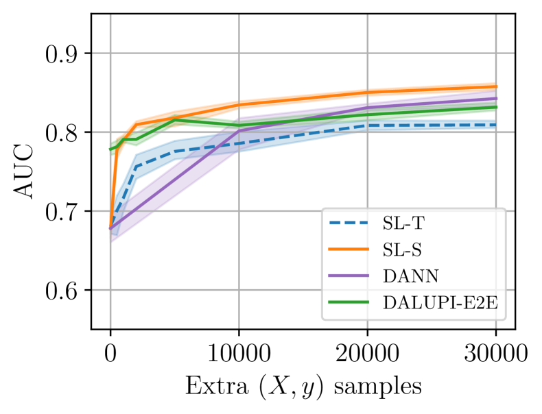
(a) Source test AUC.

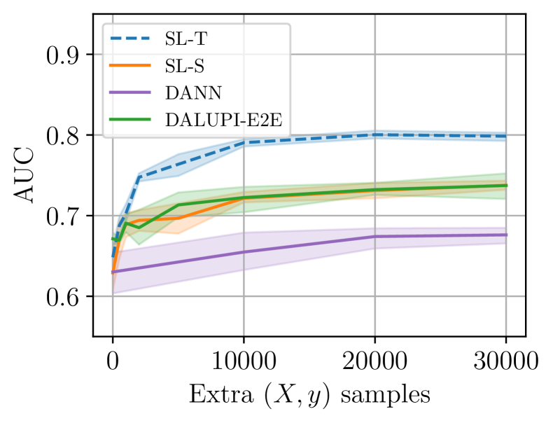
(b) Target test AUC.

Figure 6: Classification of chest X-ray images. Model performance on source (a) and target (b) domains. The AUC is averaged over the three pathologies: ATL, CM and PE. The $95\text{\,}\mathrm{\char 37\relax}$ confidence intervals are computed using bootstrapping over 5 seeds.

In Figure 5(b) in Section 5.3, we present AUC for the pathology CM when additional training data are added. In Figure 6, we show the average AUC when additional training data of up to $30\,000\text{\,}\mathrm{s}$amples are added. We see that, once given access to a much larger amount of labeled samples, SL-S and DALUPI-E2E perform comparably in the target domain.

Appendix C Proof of Proposition 2

Proposition 2.

Assume that $\mathcal{G}$ comprises M-Lipschitz mappings from the privileged information space $\mathcal{W}\subseteq\mathbb{R}^{d_{W}}$ to $\mathcal{Y}$. Further, assume that both the ground truth privileged information $W$ and label $Y$ are deterministic in $X$ and $W$ respectively. Let $\rho$ be the domain density ratio of $W$ and let Assumptions 1–3 (Covariate shift, Overlap and Sufficiency) hold w.r.t. $W$. Further, let the loss $L$ be uniformly bounded by some constant $B$ and let $d$ and $d^{\prime}$ be the pseudo-dimensions of $\mathcal{G}$ and $\mathcal{F}$ respectively. Assume that there are $n$ observations each from the source (labeled) and target (unlabeled) domains. Then, with $L$ the squared Euclidean distance, for any $h=f\circ g\in\mathcal{F}\times\mathcal{G}$, w.p. at least $1-\delta$,

$$\frac{R_{\mathcal{T}}(h)}{2} \leq\hat{R}^{Y,\rho}_{\mathcal{S}}(g)+M^{2}\hat{R}^{W}_{\mathcal{T}}(f)$$

$$+2^{5/4}\sqrt{d_{2}(\mathcal{T}\|\mathcal{S})}\sqrt[\frac{3}{8}]{\frac{d\log\frac{2ne}{d}+\log\frac{4}{\delta}}{n}}$$

$$+d_{\mathcal{W}}BM^{2}\left(\sqrt{\frac{2d^{\prime}\log\frac{en}{d^{\prime}}}{n}}+\sqrt{\frac{\log\frac{d_{\mathcal{W}}}{\delta}}{2n}}\right).$$

Proof.

Decomposing the risk of $h\circ\phi$ , we get

$$R_{\mathcal{T}}(h)=\mathbb{E}_{\mathcal{T}}[(g(f(X))-Y)^{2}]$$

$$\leq 2\mathbb{E}_{\mathcal{T}}[(g(W)-Y)^{2}+(g(f(X))-g(W))^{2}]$$

$$\leq 2\mathbb{E}_{\mathcal{T}}[(g(W)-Y)^{2}+M^{2}\|f(X))-g(W)\|^{2}]$$

$$\leq 2\mathbb{E}_{\mathcal{T}}[(g(W)-Y)^{2}]+2M^{2}\mathbb{E}_{\mathcal{T}}[\|(f(X)-W)\|^{2}]$$

$$=2R^{Y}_{\mathcal{T}}(g)+2M^{2}R^{W}_{\mathcal{T}}(f)=2\underbrace{R^{Y,\rho}_{S}(g)}_{(I)}+2M^{2}\underbrace{R^{W}_{\mathcal{T}}(f)}_{(II)}.$$

The first inequality follows from the relaxed triangle inequality, the second inequality from the Lipschitz property and the third equality from Overlap and Covariate shift. We will bound these quantities separately starting with $(I)$.

We assume that the pseudo-dimension of $\mathcal{G}$, $d$ is bounded. Further, we assume that the second moment of the density ratios, equal to the Rényi divergence $d_{2}(\mathcal{T}\|\mathcal{S})=\Sigma_{w\in cG}\mathcal{T}(w)\frac{\mathcal{T}(w)}{\mathcal{S}(w)}$ are bounded and that the density ratios are non-zero for all $w\in\mathcal{G}$. Let $D_{1}=\{w_{i},y_{i}\}_{i=0}^{n}$ be a dataset drawn i.i.d from the source domain. Then by application of Theorem 3 from Cortes et al. (2010) we obtain with probability $1-\delta$ over the choice of $D_{1}$,

$$(I)=R^{Y,\rho}_{S}(g)\leq\hat{R}^{Y,\rho}_{S}(g)+2^{5/4}\sqrt{d_{2}(\mathcal{T}\|\mathcal{S})}\sqrt[3/8]{\frac{d\log\frac{2ne}{d}+\log\frac{4}{\delta}}{n}}$$

Now for $(II)$ we treat each component of $w\in\mathcal{W}$ as a regression problem independent from all the others. So we can therefore write the risk as the sum of the individual component risks

$$R^{W}_{\mathcal{T}}(f)=\Sigma_{i=1}^{d_{\mathcal{W}}}R^{W}_{\mathcal{T},i}(f)$$

Let the pseudo-dimension of $\mathcal{F}$ be denoted $d$, $D_{2}=\{x_{i},w_{i}\}_{i=0}^{n}$ be a dataset drawn i.i.d from the target domain. Then, using theorem 11.8 from Mohri et al. (2018) we have that for any $\delta>0$, with probability at least $1-\delta$ over the choice of $D_{2}$, the following inequality holds for all hypotheses $f\in\mathcal{F}$ for each component risk

$$R^{W}_{\mathcal{T},i}(f) \leq\hat{R}^{W}_{\mathcal{T},i}(f)+B\left(\sqrt{\frac{2d^{\prime}\log\frac{en}{d^{\prime}}}{n}}+\sqrt{\frac{\log\frac{1}{\delta}}{2n}}\right)$$

We then simply make all the bounds hold simultaneously by applying the union bound and having it so that each bound must hold with probability $1-\frac{\delta}{d_{\mathcal{W}}}$ which results in

$$R^{W}_{\mathcal{T}}(f) =\Sigma_{i=1}^{d_{\mathcal{W}}}R^{W}_{\mathcal{T},i}(f)\leq\Sigma_{i=1}^{d_{\mathcal{W}}}\hat{R}^{W}_{\mathcal{T},i}(f)+\Sigma_{i=1}^{d_{\mathcal{W}}}B\left(\sqrt{\frac{2d^{\prime}\log\frac{en}{d^{\prime}}}{n}}+\sqrt{\frac{\log\frac{d_{\mathcal{W}}}{\delta}}{2n}}\right)$$

$$=\hat{R}^{W}_{\mathcal{T}}(f)+d_{\mathcal{W}}B\left(\sqrt{\frac{2d^{\prime}\log\frac{en}{d^{\prime}}}{n}}+\sqrt{\frac{\log\frac{d_{\mathcal{W}}}{\delta}}{2n}}\right)$$

Combination of these two results then yield the proposition statement.

Consistency follows as $Y$ is a deterministic function of $W$ and $W$ is a deterministic fundtion of $X$ and both $\mathcal{H}$ and $\mathcal{F}$ are well-specified. Thus both empirical risks and sample complexity terms will converge to 0 in the limit of infinite samples. ∎

Appendix D t-SNE plot for digit classification experiment

We present some t-SNE plots for the SL-S model for the digit classification experiment in Figure 7 and 8. We clearly see that when the skew is low the target is well separated. However, with full correlation between the label and the background we see that the separation is lost. The perplexity is set to 100 when producing these plots.

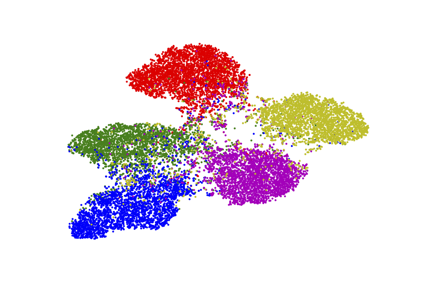
(a) t-SNE plot of the source test set, $\epsilon=0.2$.

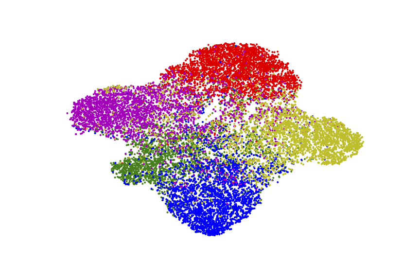
(b) t-SNE plot of the target test set, $\epsilon=0.2$.

Figure 7: t-SNE when the skew is $\epsilon=0.2$.

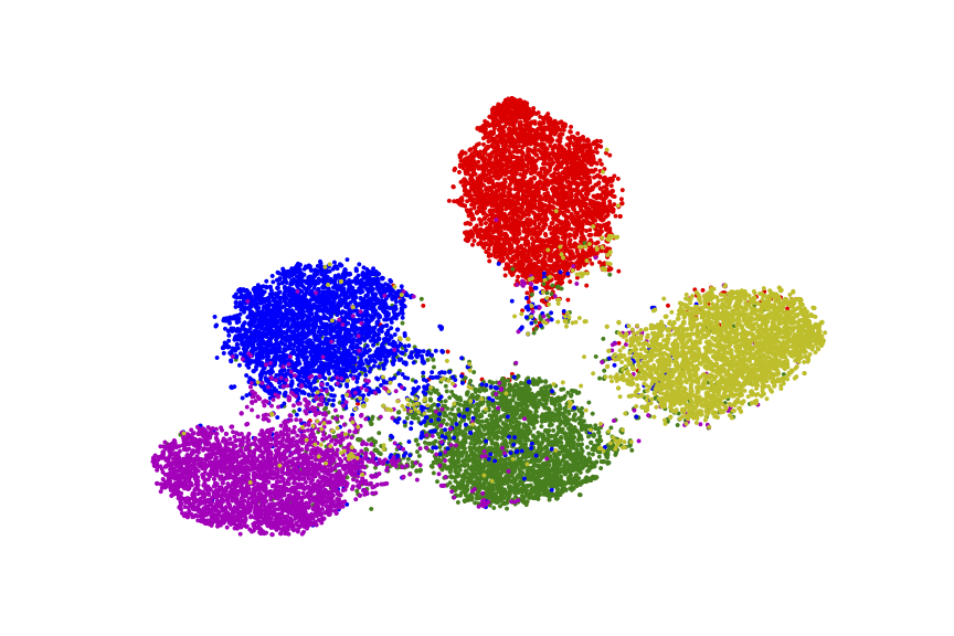
(a) t-SNE plot of the source test set, $\epsilon=1$.

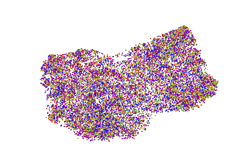
(b) t-SNE plot of the target test set, $\epsilon=1$.

Figure 8: t-SNE when the skew is $\epsilon=1$.

References

- Beery et al. (2018) Beery, S., Van Horn, G., and Perona, P. Recognition in terra incognita. In Proceedings of the European conference on computer vision (ECCV), pp. 456–473, 2018.
- Ben-David & Urner (2012) Ben-David, S. and Urner, R. On the hardness of domain adaptation and the utility of unlabeled target samples. In International Conference on Algorithmic Learning Theory, pp. 139–153. Springer, 2012.
- Ben-David et al. (2006) Ben-David, S., Blitzer, J., Crammer, K., and Pereira, F. Analysis of representations for domain adaptation. Advances in neural information processing systems, 19, 2006.
- Breitholtz & Johansson (2022) Breitholtz, A. and Johansson, F. D. Practicality of generalization guarantees for unsupervised domain adaptation with neural networks. Transactions on Machine Learning Research, 2022.
- Chen et al. (2017) Chen, Y., Jin, X., Feng, J., and Yan, S. Training group orthogonal neural networks with privileged information. In Proceedings of the Twenty-Sixth International Joint Conference on Artificial Intelligence, IJCAI-17, pp. 1532–1538, 2017.
- Cortes et al. (2010) Cortes, C., Mansour, Y., and Mohri, M. Learning bounds for importance weighting. In Lafferty, J., Williams, C., Shawe-Taylor, J., Zemel, R., and Culotta, A. (eds.), Advances in Neural Information Processing Systems, volume 23. Curran Associates, Inc., 2010.
- Feyereisl & Aickelin (2012) Feyereisl, J. and Aickelin, U. Privileged information for data clustering. Information Sciences, 194:4–23, 2012.
- Ganin et al. (2016) Ganin, Y., Ustinova, E., Ajakan, H., Germain, P., Larochelle, H., Laviolette, F., Marchand, M., and Lempitsky, V. Domain-Adversarial Training of Neural Networks. arXiv:1505.07818 [cs, stat], May 2016. arXiv: 1505.07818.
- Girshick (2015) Girshick, R. Fast r-cnn. In Proceedings of the IEEE international conference on computer vision, pp. 1440–1448, 2015.
- He et al. (2016) He, K., Zhang, X., Ren, S., and Sun, J. Deep residual learning for image recognition. In 2016 IEEE Conference on Computer Vision and Pattern Recognition (CVPR), pp. 770–778, 2016.
- Hinton et al. (2015) Hinton, G. E., Vinyals, O., and Dean, J. Distilling the knowledge in a neural network. ArXiv, abs/1503.02531, 2015.
- Hoffman et al. (2016) Hoffman, J., Gupta, S., and Darrell, T. Learning with Side Information through Modality Hallucination. In 2016 IEEE Conference on Computer Vision and Pattern Recognition (CVPR), pp. 826–834, Las Vegas, NV, USA, June 2016. IEEE.
- Irvin et al. (2019) Irvin, J., Rajpurkar, P., Ko, M., Yu, Y., Ciurea-Ilcus, S., Chute, C., Marklund, H., Haghgoo, B., Ball, R., Shpanskaya, K., et al. Chexpert: A large chest radiograph dataset with uncertainty labels and expert comparison. In Proceedings of the AAAI conference on artificial intelligence, volume 33, pp. 590–597, 2019.
- Johansson et al. (2019) Johansson, F. D., Sontag, D., and Ranganath, R. Support and invertibility in domain-invariant representations. In The 22nd International Conference on Artificial Intelligence and Statistics, pp. 527–536. PMLR, 2019.
- Jung & Johansson (2022) Jung, B. and Johansson, F. D. Efficient learning of nonlinear prediction models with time-series privileged information. In Advances in Neural Information Processing Systems, 2022.
- Karlsson et al. (2021) Karlsson, R., Willbo, M., Hussain, Z., Krishnan, R. G., Sontag, D. A., and Johansson, F. D. Using time-series privileged information for provably efficient learning of prediction models. In Proceedings of The 25th International Conference on Artificial Intelligence and Statistics 2022, 2021.
- Krizhevsky (2009) Krizhevsky, A. Learning multiple layers of features from tiny images. Technical report, 2009.
- Lecun (1998) Lecun, Y. Gradient-Based Learning Applied to Document Recognition. proceedings of the IEEE, 86(11):47, 1998.
- Li et al. (2022) Li, Y., Sun, H., and Yan, W. Domain adaptive twin support vector machine learning using privileged information. Neurocomputing, 469:13–27, 2022.
- Lin et al. (2014) Lin, T.-Y., Maire, M., Belongie, S., Hays, J., Perona, P., Ramanan, D., Dollar, P., and Zitnick, L. Microsoft coco: Common objects in context. In ECCV. European Conference on Computer Vision, September 2014.
- Lin et al. (2017) Lin, T.-Y., Dollár, P., Girshick, R., He, K., Hariharan, B., and Belongie, S. Feature pyramid networks for object detection. In Proceedings of the IEEE conference on computer vision and pattern recognition, pp. 2117–2125, 2017.
- Long et al. (2013) Long, M., Wang, J., Ding, G., Sun, J., and Yu, P. S. Transfer feature learning with joint distribution adaptation. In Proceedings of the 2013 IEEE International Conference on Computer Vision, ICCV ’13, pp. 2200–2207, USA, 2013. IEEE Computer Society.
- Lopez-Paz et al. (2016) Lopez-Paz, D., Bottou, L., Schölkopf, B., and Vapnik, V. Unifying distillation and privileged information. In International Conference on Learning Representations (ICLR 2016), 2016.
- Mohri et al. (2018) Mohri, M., Rostamizadeh, A., and Talwalkar, A. Foundations of Machine Learning. MIT Press, second edition, 2018.
- Motiian (2019) Motiian, S. Domain Adaptation and Privileged Information for Visual Recognition. phdthesis, https://researchrepository.wvu.edu/etd/6271, 2019. Graduate Theses, Dissertations, and Problem Reports. 6271.
- Orihashi et al. (2020) Orihashi, S., Ihori, M., Tanaka, T., and Masumura, R. Unsupervised Domain Adaptation for Dialogue Sequence Labeling Based on Hierarchical Adversarial Training. In Interspeech 2020, pp. 1575–1579. ISCA, October 2020.
- Pearl & Bareinboim (2011) Pearl, J. and Bareinboim, E. Transportability of causal and statistical relations: A formal approach. In Twenty-fifth AAAI conference on artificial intelligence, 2011.
- Pechyony & Vapnik (2010) Pechyony, D. and Vapnik, V. On the theory of learnining with privileged information. In Advances in Neural Information Processing Systems, volume 23. Curran Associates, Inc., 2010.
- Ren et al. (2016) Ren, S., He, K., Girshick, R., and Sun, J. Faster r-cnn: Towards real-time object detection with region proposal networks. IEEE Transactions on Pattern Analysis and Machine Intelligence, 39(6):1137–1149, 2016.
- Robinson et al. (2020) Robinson, J., Jegelka, S., and Sra, S. Strength from Weakness: Fast Learning Using Weak Supervision. In Proceedings of the 37th International Conference on Machine Learning, pp. 8127–8136. PMLR, November 2020.
- Sarafianos et al. (2017) Sarafianos, N., Vrigkas, M., and Kakadiaris, I. A. Adaptive svm+: Learning with privileged information for domain adaptation. In Proceedings of the IEEE International Conference on Computer Vision (ICCV) Workshops, Oct 2017.
- Shaikh et al. (2020) Shaikh, T. A., Ali, R., and Beg, M. M. S. Transfer learning privileged information fuels CAD diagnosis of breast cancer. Machine Vision and Applications, 31(1):9, February 2020.
- Sharmanska et al. (2014) Sharmanska, V., Quadrianto, N., and Lampert, C. H. Learning to Transfer Privileged Information. arXiv:1410.0389 [cs, stat], October 2014. arXiv: 1410.0389.
- Shen et al. (2022) Shen, K., Jones, R. M., Kumar, A., Xie, S. M., Haochen, J. Z., Ma, T., and Liang, P. Connect, not collapse: Explaining contrastive learning for unsupervised domain adaptation. In Chaudhuri, K., Jegelka, S., Song, L., Szepesvari, C., Niu, G., and Sabato, S. (eds.), Proceedings of the 39th International Conference on Machine Learning, volume 162 of Proceedings of Machine Learning Research, pp. 19847–19878. PMLR, 17–23 Jul 2022.
- Shimodaira (2000) Shimodaira, H. Improving predictive inference under covariate shift by weighting the log-likelihood function. Journal of statistical planning and inference, 90(2):227–244, 2000.
- Silva et al. (2010) Silva, C., Vieira, A., Gaspar-Cunha, A., and Carvalho das Neves, J. Financial distress model prediction using SVM+. In Proceedings of the International Joint Conference on Neural Networks, pp. 1–7, July 2010.
- Sugiyama et al. (2012) Sugiyama, M., Suzuki, T., and Kanamori, T. Density Ratio Estimation in Machine Learning. Cambridge books online. Cambridge University Press, 2012.
- Tietz et al. (2017) Tietz, M., Fan, T. J., Nouri, D., Bossan, B., and skorch Developers. skorch: A scikit-learn compatible neural network library that wraps PyTorch, July 2017.
- Vapnik & Izmailov (2015) Vapnik, V. and Izmailov, R. Learning Using Privileged Information: Similarity Control and Knowledge Transfer. Journal of Machine Learning Research, 16:2023–2049, 2015.
- Vapnik & Vashist (2009) Vapnik, V. and Vashist, A. A new learning paradigm: Learning using privileged information. Neural Networks, 22(5):544–557, July 2009.
- Vu et al. (2019) Vu, T.-H., Jain, H., Bucher, M., Cord, M., and Pérez, P. P. Dada: Depth-aware domain adaptation in semantic segmentation. In 2019 IEEE/CVF International Conference on Computer Vision (ICCV), pp. 7363–7372, 2019.
- Wang et al. (2017) Wang, X., Peng, Y., Lu, L., Lu, Z., Bagheri, M., and Summers, R. M. Chestx-ray8: Hospital-scale chest x-ray database and benchmarks on weakly-supervised classification and localization of common thorax diseases. In Proceedings of the IEEE conference on computer vision and pattern recognition, pp. 2097–2106, 2017.
- Wu et al. (2019) Wu, Y., Winston, E., Kaushik, D., and Lipton, Z. Domain adaptation with asymmetrically-relaxed distribution alignment. In International conference on machine learning, pp. 6872–6881. PMLR, 2019.
- Zech et al. (2018) Zech, J. R., Badgeley, M. A., Liu, M., Costa, A. B., Titano, J. J., and Oermann, E. K. Variable generalization performance of a deep learning model to detect pneumonia in chest radiographs: a cross-sectional study. PLoS medicine, 15(11):e1002683, 2018.
- Zhao et al. (2019) Zhao, H., Des Combes, R. T., Zhang, K., and Gordon, G. On learning invariant representations for domain adaptation. In International Conference on Machine Learning, pp. 7523–7532. PMLR, 2019.