Strong decays of charmonium-like state Y(4230)

Abstract

Strong decays of the charmonium-like state $Y(4320)$ have been studied in the framework of the covariant confined quark model. The resonance $Y$ has been interpreted as a four-quark state of the molecular type. We evaluate the hidden-charm decay width of $Y$ to a vector and a scalar, with the latter decaying subsequently to a pair of charged pseudoscalar states. The strong decay modes $Y\!\to\!\pi^{+}\pi^{-}J/\Psi$ and $Y\!\to\!K^{+}K^{-}J/\Psi$ have been studied by involving the scalar resonance state $f_{0}(980)$. We have calculated the fractal widths of the related strong decays and the branching ratio ${\cal B}(Y\!\to\!K^{+}K^{-}J/\Psi)$ / ${\cal B}(Y\!\to\!\pi^{+}\pi^{-}J/\Psi)$,  recently determined by the BESIII collaboration. The estimated branching ratio and calculated fractal strong decay widths are in good agreement with the latest experimental data, favoring the molecular representation of the $Y(4320)$ state.

I   Introduction

During the past years, several unusual states were observed in the course of experimentally establishing the heavy meson spectrum. They possess a common feature - a minimal constituent quark-antiquark model does not work for these states. One of these unusual states is the $Y(4230)$ (also known as $\psi(4260)$ and $Y(4260)$) and this resonance still needs solid experimental study. Historically, the data analysis of the mass spectrum of $\pi^{+}\pi^{-}J\!/\!\psi$ in production $e^{+}e^{-}\to\gamma_{\rm ISR}\,\pi^{+}\pi^{-}J\!/\!\psi$ by the BaBar Collaboration observed a broad resonance around $4.26$ GeV Aubert:2005rm . The spin-parity $J^{PC}=1^{--}$ indicates a possible charmonium state, but its mass did not match any known mass of charmonium states. Along with the strong coupling to $\pi^{+}\pi^{-}J\!/\!\psi$, no evidence was found for coupling to any open charm decay modes.

Earlier studies suggested that the $Y(4230)$ state is not a conventional state of charmonium Brambilla:2010cs . Then, $Y$ has been interpreted as a charmonium-hybrid state in Refs. Zhu:2005hp ; Kou:2005gt ; Close:2005iz .

An interpretation of $Y(4260)$ as the first orbital excitation of diquark-antidiquark state $([cs][\bar{c}\bar{s}])$ was proposed in Ref.  Maiani:2005pe by assuming a dominant decay to $D_{s}\bar{D}_{s}$.

Another way to look at $Y(4260)$ is as a $\chi_{c1}-\rho^{0}$ molecule was developed in  Liu:2005ay . Then, the $Y(4260)\to\pi^{+}\pi^{-}J\!/\!\psi$ decay width should be larger than $Y(4260)\to D\bar{D}$ that has not been observed. The absence of the $Y(4260)$ in the decays with open charm can be clearly explained by an assumption considering the $Y$ as a $D\bar{D}_{1}$ molecular state Wang:2013cya . In the framework of the molecular-type interpretation, some hidden-charm and charmed pair decay channels via intermediate $DD_{1}$ meson loops have been investigated  Li:2013yla . Considering $DD_{1}$, a weakly bound state, a two-body decay $Y(4260)\to Z_{c}(3900)+\pi$ has been studied. Furthermore, the decay mode $Y(4260)\to J\!/\!\psi+\pi^{+}\pi^{-}$ was also calculated Dong:2013kta .

The cross sections of $e^{+}e^{-}\rightarrow K^{+}K^{-}J/\psi$ have more recently been measured by using 15.6 fb^-1 gathered with the BESIII detector Ablikim:2022 . The mass and width of this structure are measured to be ($4225.3~{}\pm~{}2.3~{}\pm~{}21.5$) MeV and ($72.9\pm 6.1\pm 30.8$) MeV, respectively. They align with the standards set forth for $Y(4230)$.

Furthermore, the ratio of the branching fractions of $Y(4230)$ decaying into $K\bar{K}J/\psi$ and $\pi\pi J/\psi$ modes is determined Ablikim:2022 to be

$$0.02<\frac{\mathcal{B}(Y(4230)\to K^{+}K^{-}J/\psi)}{\mathcal{B}(Y(4230)\to\pi^{+}\pi^{-}J/\psi)}<0.26\,,$$

where ranges are determined from the eight combinations of multiple solutions in the two measurements and the large ambiguity is primarily due to the multiple solutions in the $\pi^{+}\pi^{-}J\!/\!\psi$ measurement. However, the difficulties in reaching a judgment before finding the physics solution in the measurements has been highlighted, particularly for the $\pi^{+}\pi^{-}J\!/\!\psi$ mode.

In the present paper we investigate strong decays of the $Y(4320)$ resonance in the framework of the covariant confined quark model (CCQM) Branz:2009cd proposed and developed by us last decade. The model implements effective quark confinement with convolutions of local quark propagators and vertex functions accompanied by an infrared cutoff of the scale integration that prevents any singularities in matrix elements. We have applied the CCQM to multiquark meson structure, form factors and angular decay characteristics of light and heavy baryons. Possible new physics effects in the exclusive decays of $\bar{B}^{0}$ and transitions of $\Lambda_{b}$ have been studied in some extension of the Standard Model by taking into account right-handed vector (axial), left- and right-handed (pseudo)scalar, and tensor current contributions. Inspired by recent measurements we have studied the radiative decays of charmonium states below the $D{\bar{D}}$ threshold by introducing only one adjustable parameter common for the six charmonium states. The obtained results were in good agreement with the latest data, we also predicted a more narrow full width for the $h_{c}$ charmonium Ganbold:2021 . In our papers devoted to description of the multi-quark states Refs.Dubnicka:2011mm , first, we have treated the $X(3872)$ meson as a diquark-antidiquark bound state. In  Goerke:2016hxf we have employed a molecular-type four-quark current to describe the decays of the $Z_{c}(3900)$ state and shown that a molecular-type current can give the decay width values in accordance with the experiment. By using molecular-type four-quark currents for the recently observed resonances $Z_{b}(10610)$ and $Z_{b}(10650)$, we have calculated in Ref. Goerke:2017svb their two-body decay rates into a bottomonium state plus a light meson as well as into B-meson pairs. A brief sketch of our findings may be found in Ref. Ivanov:2018ayq . We have investigated two interpolating currents for the $Y(4260)$ resonance: the molecular-type current and the tetraquark one Dubnicka:2020 . We demonstrated that the mode $Y\to Z^{+}_{c}+\pi^{-}$ was enhanced in both approaches when compared to open-charm modes.

The paper is organized as follows. A brief description of the CCQM and the general formalism for describing $Y(4260)$ as four quark molecular state are give in Sec. II. In Sec. III we calculate the related amplitude and width of the strong decay $Y\to f_{0}+J\!/\!\psi$. Sec. IV is dedicated to the investigation of two decays: $f_{0}\!\to\!\pi^{+}\!+\!\pi^{-}$ and $f_{0}\!\to\!K^{+}\!+\!K^{-}$ with related formulas for the Lorentz form factors, matrix elements, phase volumes and fractional decay widths. In the next, Sec. V, we study the strong decays $Y(4230)\to K^{+}K^{-}J\!/\!\psi$ and $Y(4230)\to\pi^{+}\pi^{-}J\!/\!\psi$ occuring via intermediate scalar resonance $f_{0}(980)$ in different ways: by using the narrow-width approximation, its improved modification and full integration over kinematically allowed resonance momentum. In Sec. VI we discuss the obtained results by comparing them with latest experimental data.

II   Approach

The covariant confining quark model (CCQM)  Branz:2009cd represents an effective quantum field treatment of hadronic effects and derived from Lorentz invariant non-local Lagrangian in which a hadron is coupled to its constituent quarks. Hereby, hadrons are characterized by size parameters $\Lambda_{H}$ dictating the strength of the quark-hadron coupling. This mechanism is done by using so-called compositeness condition  Salam:1962ap ; Weinberg:1962hj requiring the wave-function renormalization constant of the hadron to be zero $Z_{H}=0$. This condition reduces the number of free parameters (i.e. couplings) and guarantues a correct description of bound states as dressed (with no overlap with bare states). The hadron-quark interaction vertices are given by a Gaussian-type functions. An analytic built-in confinement, based on a cutoff in the integration space of Schwinger parameters of quark propagators, removes all divergencies and the model can be used for description of arbitrary heavy hadrons.

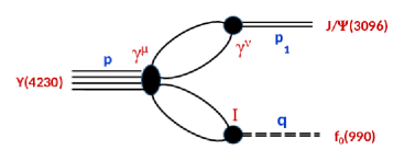
Figure 2: Leading-order Feynman diagram for decay $Y\to J\!/\!\psi+f_{0}$.

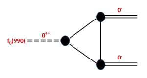
Figure 3: Leading-order Feynman diagram for strong decay of $f_{0}$ into two pseudoscalar mesons.

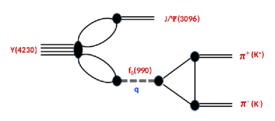
Figure 4: Leading-order Feynman diagram for decays $Y\to\pi^{+}\pi^{-}J\!/\!\psi$ and $Y\to K^{+}K^{-}J\!/\!\psi$.

Below we use the CCQM to investigate three modes of the strong $Y(4260)$-decay with hidden-charm combinations as follows: $Y\to J\!/\!\psi\,f_{0}$, $Y\to J\!/\!\psi\,K^{+}\,K^{-}$ and $Y\to J\!/\!\psi\,\pi^{+}\,\pi^{-}$, shown in Figs. 2-5.

According to the CCQM, the effective interaction Lagrangian describing the coupling of the meson $Y(4230)$ to its constituent quarks can be written in the form:

$${\cal L}_{\rm int}=g_{Y}\,Y_{\mu}(x)\cdot J^{\mu}_{Y}(x)+\text{H.c.}$$ (1)

Since the neutral state $Y(4230)$ with the quantum numbers $I^{G}(J^{PC})=0^{-}(1^{--})$ cannot be successfully described within the framework of any quark-antiquark bound state, we introduce the interpolating four-quark molecular-type current as follows:

$$J_{Y}^{\mu}=\frac{1}{\sqrt{2}}\left\{(\bar{q}\gamma_{5}c)(\bar{c}\gamma^{\mu}\gamma_{5}q)+(\gamma_{5}\leftrightarrow\gamma^{\mu}\gamma_{5})\right\}.$$ (2)

The corresponding nonlocal generalization of the four-quark current within the CCQM reads

$$J_{Y}^{\mu}(x) = \int\!dx_{1}\ldots\int\!dx_{4}\delta\left(x-\sum\limits_{i=1}^{4}w_{i}x_{i}\right)\Phi_{\,Y}\Big{(}\sum\limits_{i<j}(x_{i}-x_{j})^{2}\Big{)}J_{Y_{non}}^{\mu}(x_{1},\ldots,x_{4}),$$ (3)

$$J_{Y_{non}}^{\mu} = \tfrac{1}{\sqrt{2}}\Big{\{}(\bar{q}(x_{3})\gamma_{5}c(x_{1}))\cdot(\bar{c}(x_{2})\gamma^{\mu}\gamma_{5}q(x_{4}))+(\gamma_{5}\leftrightarrow\gamma^{\mu}\gamma_{5})\Big{\}},\qquad(q=u,d),$$

where the reduced quark masses $w_{i}=m_{i}/\sum_{j=1}^{4}m_{j}$ are specified for $m_{1}=m_{2}=m_{c}$ and $m_{3}=m_{4}=m_{q}$. Hereby, we neglect the isospin violation in the $u-d$ sector, i.e. $m_{u}=m_{d}=m_{q}$. The numbering of the coordinates $x_{i}$ is chosen such that one has a convenient arrangement of vertices and propagators in the Feynman diagrams to be calculated.

The translationally invariant four-quark vertex function reads:

$$\Phi_{Y}\Big{(}\sum\limits_{i<j}(x_{i}-x_{j})^{2}\Big{)}=\prod\limits_{i=1}^{3}\int\!\!\frac{d^{4}q_{i}}{(2\pi)^{4}}\,e^{-iq_{i}(x_{i}-x_{4})}\widetilde{\Phi}_{Y}(-Q^{2}),\qquad Q^{2}=\frac{1}{2}\sum\limits_{i\leq j}q_{i}q_{j}.$$ (4)

The Fourier transform of the translationally invariant vertex function in momentum space is required to fall off in the Euclidean region in order to provide the ultraviolet convergence of the loop integrals. We use a simple Gaussian form as follows:

$$\widetilde{\Phi}_{Y}(-Q^{2})=\exp(Q^{2}/\Lambda^{2}_{Y})\,,$$ (5)

where $\Lambda_{Y}>0$ is an adjustable hadron size-related parameter of the CCQM. In fact, any choice for $\widetilde{\Phi}_{Y}$ is appropriate as long as it falls off sufficiently fast in the ultraviolet region to render the corresponding Feynman diagrams ultraviolet finite.

The renormalized coupling constant $g_{Y}$ in Eq. (1) is strictly determined by the compositeness condition (see Ref. Branz:2009cd for details) as follows:

$$Z_{Y}=1-g^{2}_{Y}\,\frac{d}{dp^{2}}\widetilde{\Pi}_{Y}(p^{2})=0,\qquad p^{2}=M^{2}_{Y},$$ (6)

where $\Pi_{Y}(p^{2})$ is the diagonal (scalar) part of the vector-meson mass operator defined in momentum space

$$\widetilde{\Pi}_{Y}(p^{2})=\frac{1}{3}\left(g_{\mu\nu}-\frac{p_{\mu}p_{\nu}}{p^{2}}\right)\widetilde{\Pi}^{\mu\nu}_{Y}(p).$$ (7)

Therefore, any bare states are removed totally from consideration, the mass and wave function of the hadron are renormalized, and the physical state is dressed.

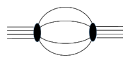
Figure 1: Feynman diagram for $Y(4230)$ mass operator

The Fourier transform of the mass operator for the four-quark state $Y$ is written as

$$\widetilde{\Pi}_{Y}^{\mu\nu}(p) = \frac{N_{c}^{2}}{2}\,\prod\limits_{i=1}^{3}\int\!\!\frac{d^{4}k_{i}}{(2\pi)^{4}i}\,\widetilde{\Phi}_{Y}^{2}\left(-(k_{1}^{2}+k_{2}^{2}+k_{3}^{2}-k_{1}k_{2}-k_{1}k_{3}+k_{2}k_{3})/2\right)$$

$$\times \Big{\{}\mbox{\rm{tr}}\left[S_{3}(\hat{k}_{3}+w_{3}\hat{p})\gamma_{5}S_{1}(\hat{k}_{1}-w_{1}\hat{p})\gamma_{5}\right]$$

$$\times\mbox{\rm{tr}}\left[S_{2}(\hat{k}_{2}+w_{2}\hat{p})\gamma^{\mu}\gamma_{5}S_{4}(-\hat{k}_{1}+\hat{k}_{2}+\hat{k}_{3}-w_{4}\hat{p})\gamma^{\nu}\gamma_{5}\right]$$

$$+\,\mbox{\rm{tr}}\left[S_{3}(\hat{k}_{3}+w_{3}\hat{p})\gamma_{5}S_{1}(\hat{k}_{1}-w_{1}\hat{p})\gamma^{\nu}\gamma_{5}\right]$$

$$\times\mbox{\rm{tr}}\left[S_{2}(\hat{k}_{2}+w_{2}\hat{p})\gamma^{\mu}\gamma_{5}S_{4}(-\hat{k}_{1}+\hat{k}_{2}+\hat{k}_{3}-w_{4}\hat{p})\gamma_{5}\right]\Big{\}}\,,\quad N_{c}=3\,.$$

For the quark propagator we use the Fock-Schwinger representation:

$$\widetilde{S}_{j}(\hat{k})=\left(m_{j}+\hat{k}\right)\intop_{0}^{\infty}d\alpha\>\exp\big{(}-\alpha\left(m_{j}^{2}-k^{2}\right)\big{)}\,.$$ (9)

Matrix elements of hadronic processes described by using Feynman quark-loop diagrams may be represented in terms of convolutions of vertex functions and quark propagators as follows:

$$\Pi^{0}\!\!=N_{c}\!\!\int_{0}^{\infty}\!\!\!dt\,t^{n-1}\!\!\int_{0}^{1}\!\!\!d^{n}\alpha\,\delta\Big{(}1\!\!-\!\!\sum_{i=1}^{n}\alpha_{i}\Big{)}f(t\alpha_{1},\ldots,t\alpha_{n}).$$ (10)

Hereby, possible branch points connected with the creation of free quarks may appear. These threshold singularities can be removed by introducing a universal infrared cutoff parameter, $\lambda$ as follows: $\!\!\int_{0}^{\infty}\!\!dt\ldots\to\int_{0}^{1/\lambda^{2}}\!\!dt\ldots$.

III   Strong decay $Y(4230)\to J\!/\!\psi+f_{0}(980)$

Consider the strong decay $Y(4230)\to J\!/\!\psi+f_{0}(980)$ represented in the leading order by the Feynman diagram in Fig.1.

The matrix element of the two-body decay of $Y$ into a vector ($V=J\!/\!\psi(3096)$) and a scalar ($S=f_{0}(980)$) reads

$${\cal M}_{YVS}={\cal M}\left(Y(p,\epsilon^{\mu}_{p})\to J\!/\!\psi(p_{1},\epsilon^{\nu}_{p_{1}})+f_{0}(q)\right)\doteq\,g_{Y}\,g_{J\!/\!\psi}\,g_{f_{0}}\,\epsilon^{\mu}_{p}\,\epsilon^{\ast\,\nu}_{p_{1}}\left(d_{A}\,p_{1}^{\mu}p^{\nu}-d_{B}\,g^{\mu\nu}(p\,p_{1})\right)\,.$$ (11)

The Lorentz form factors $d_{A}$ and $d_{B}$ in the LO are defined as follows:

$$d_{A}\,p_{1}^{\mu}p^{\nu}-d_{B}\,g^{\mu\nu}=$$ (12)

$$\frac{N_{c}^{2}}{2}\int\!\!\frac{d^{4}k_{1}}{(2\pi)^{4}i}\,\int\!\!\frac{d^{4}k_{2}}{(2\pi)^{4}i}\,\widetilde{\Phi}_{Y}\left(-Q^{2}\right)\widetilde{\Phi}_{J\!/\!\psi}\left(-\,(\ell_{1}+\ell_{2})^{2}/4\right)\widetilde{\Phi}_{f_{0}}\left(-\,(\ell_{3}+\ell_{4})^{2}/4\right)$$

$$\times \Big{\{}\mbox{\rm{tr}}\left[\gamma_{5}S_{1}(\ell_{1})\gamma^{\nu}S_{2}(\ell_{2})\gamma^{\mu}\gamma_{5}S_{4}(\ell_{4})IS_{3}(\ell_{3})\right]+\mbox{\rm{tr}}\left[\gamma^{\mu}\gamma_{5}S_{1}(\ell_{1})\gamma^{\nu}S_{2}(\ell_{2})\gamma_{5}S_{4}(\ell_{4})IS_{3}(\ell_{3})\right]\Big{\}}\,,$$

$$Q^{2}=\left[(\ell_{1}+pw_{1})^{2}+(\ell_{2}-pw_{2})^{2}+(\ell_{3}+pw_{3})^{2}+(\ell_{4}-pw_{4})^{2}\right]/2,$$

$$\ell_{1}=k_{1}-pw_{1},\quad\ell_{2}=k_{1}-pw_{1}-p_{1},\quad\ell_{3}=k_{2}-pw_{4}-q,\quad\ell_{4}=k_{2}-pw_{4}\,,$$

where $\widetilde{\Phi}_{J\!/\!\psi}(-k^{2})=\exp(k^{2}/\Lambda^{2}_{J\!/\!\psi})$ and $\widetilde{\Phi}_{f_{0}}(-k^{2})=\exp(k^{2}/\Lambda^{2}_{f_{0}})$ are vertex functions with adjustable hadron size-related parameters $\Lambda_{J\!/\!\psi}$ and $\Lambda_{f_{0}}$.

The fractional strong decay width $\Gamma(Y\!\!\to\!\!J\!/\!\psi\!+\!f_{0})$ is calculated as follows:

$$\Gamma_{YVS}\!\!\!\! =\frac{g^{2}_{Y}g^{2}_{J\!/\!\psi}g^{2}_{f_{0}}}{(2s+1)\,2\,M_{Y}}\,(p\,p_{1})^{2}\left\{(\xi\!-\!2\!+\!\xi^{-1})\,d_{A}^{2}\!+\!2\,(1\!-\!\xi)\,d_{A}d_{B}\!+\!(2\!+\!\xi)\,d_{B}^{2}\right\}\cdot\Omega_{YVS}\,,$$

$$(p\,p_{1})^{2}=(p^{2}+p_{1}^{2}-q^{2})/2\,,\qquad\xi\doteq(p\,p_{1})^{2}/(p^{2}\,p_{1}^{2})\,,$$

where $s=1$ is the spin of unpolarized particle Y(4230) and the phase volume of the decay is introduced as follows:

$$\Omega_{YVS}=\Omega_{Y\to J\!/\!\psi+f_{0}}(M_{Y}^{2},M_{J\!/\!\psi}^{2},M_{f_{0}}^{2})=\frac{1}{8\pi M_{Y}^{2}}\left[\lambda(M_{Y}^{2},M_{J\!/\!\psi}^{2},M_{f_{0}}^{2})\right]^{1/2}$$ (14)

with the Källen function $\lambda(p^{2},p_{1}^{2},q^{2})$.

IV   Strong decay of $f_{0}(980)$ into two pseudoscalar mesons

Let us consider a strong decay of a scalar particle $f_{0}(q)\to P^{+}(q_{1})+P^{-}(q_{2})$ into a pair of charged pseudoscalar mesons - either $\pi^{+}\pi^{-}$, or $K^{+}K^{-}$. Further, we use notations $P^{+}=\{\pi^{+},\,K^{+}\}$ and $P^{-}=\{\pi^{-},\,K^{-}\}$.

The matrix element of the decay takes the following form:

$${\cal M}_{SPP}=g_{f_{0}}\,g_{P^{+}}\,g_{P^{-}}\cdot d_{C}\,.$$ (15)

The corresponding Lorentz form factor of the decay in the LO reads

$$d_{C} = \frac{N_{c}}{2}\int\!\!\frac{d^{4}k}{(2\pi)^{4}i}\,\widetilde{\Phi}_{f_{0}}\left(-k^{2}\right)\widetilde{\Phi}_{P^{+}}\left(-\,(\ell_{2}+\ell_{3}+q_{1}(w_{s}-w_{q}))^{2}/4\right)$$ (16)

$$\times \widetilde{\Phi}_{P^{-}}\left(-\,(\ell_{1}+\ell_{3}-q_{2}(w_{s}-w_{q}))^{2}/4\right)\mbox{\rm{tr}}\left[\gamma_{5}S_{1}(\ell_{1})IS_{2}(\ell_{2})\gamma_{5}S_{3}(\ell_{3})\right]\,,$$

where $\ell_{1}=k-q/2,\quad\ell_{2}=k+q/2,\quad\ell_{3}=k-q_{1}/2+q_{2}/2$ and $\widetilde{\Phi}_{f_{0}}(-k^{2})=\exp(k^{2}/\Lambda_{f_{0}})$, $\widetilde{\Phi}_{P^{+}}(-k^{2})=\exp(k^{2}/\Lambda_{P^{+}})$, $\widetilde{\Phi}_{P^{-}}(-k^{2})=\exp(k^{2}/\Lambda_{P^{-}})$ with corresponding ’size’ parameters $\Lambda_{f_{0}}$, $\Lambda_{P^{+}}$ and $\Lambda_{P^{-}}$.

The fractional strong decay widths is calculated as follows:

$$\Gamma_{SPP}=\Gamma(f_{0}\!\to\!P^{+}\!+\!P^{-})=\frac{g_{f_{0}}^{2}\,g_{P^{+}}^{2}\,g_{P^{-}}^{2}}{2\cdot 2\,M_{S}}\cdot d_{C}^{2}\cdot\Omega_{SPP}\,,$$ (17)

where the phase volume of the decay is introduced as follows:

$$\Omega_{SPP}=\Omega_{f_{0}\!\to\!P^{+}\!+\!P^{-}}(M_{f_{0}}^{2},M_{P^{+}}^{2},M_{P^{-}}^{2})=\frac{1}{8\pi M_{f_{0}}^{2}}\left[\lambda(M_{f_{0}}^{2},M_{P^{+}}^{2},M_{P^{-}}^{2})\right]^{1/2}$$ (18)

with the Källen function $\lambda(q^{2},q_{1}^{2},q_{2}^{2})$.

V   Strong decays of $Y(4230)\to K^{+}K^{-}J\!/\!\psi$ and $Y(4230)\to\pi^{+}\pi^{-}J\!/\!\psi$

We consider the following sequential two-body decays: first the four-quark charmonium-like state decays into the vector charmonium $J\!/\!\psi(3096)$ and the scalar resonance $f_{0}(980)$, then, $f_{0}$ decays into two charged pseudoscalar mesons - either $\pi^{+}\pi^{-}$, or $K^{+}K^{-}$.

The corresponding decay width is given by calculating an integral:

$$\Gamma(Y\!\to\!P^{+}P^{-}J\!/\!\psi)=\frac{1}{24M_{Y}}$$ (19)

$$\times \!\!\!\!\!\!\!\!\int\limits_{q^{2}_{min(P^{+}P^{-})}}^{q^{2}_{max}}\!\!\!\!\!\!dq^{2}\,\left[{\cal M}_{YVS}(q^{2})\right]^{2}\,\Omega_{YVS}(q^{2})\,BW(q^{2})\,\frac{1}{\sqrt{q^{2}}}\,\left[{\cal M}_{SPP}(q^{2})\right]^{2}\,\Omega_{SPP}(q^{2})\,$$

where the integration regions are bound by the corresponding kinematic limits.

The Breit-Wigner resonance distribution function is introduced as follows:

$$BW(q^{2})=\frac{1}{\pi}\frac{M_{S}}{(q^{2}-M_{S}^{2})^{2}+(M_{S}\Gamma_{S})^{2}}\,,\qquad\int\limits_{-\infty}^{+\infty}\!\!dq^{2}\,BW(q^{2})=\frac{1}{\Gamma_{S}}\,.$$ (20)

Below we calculate the branching ratio of strong decays with hidden charms, ${\cal B}(Y\!\to\!K^{+}K^{-}J\!/\!\psi)$ / ${\cal B}(Y\!\to\!\pi^{+}\pi^{-}J\!/\!\psi)$, via resonance state $f_{0}(980)$ in different ways, namely, by using the narrow-width approximation (NWA), its phase-space improved modification (PSINWA) and direct integration over kinematically allowed momentum of the resonance.

V.1 Narrow Width Approximation (NWA)

The integration over $q^{2}$ in Eq.(19) may be directly calculated by numerical means.

However, taking into account the latest data ($\Gamma_{f_{0}}=10\div 100$ MeV and $M_{f_{0}}=990$ MeV) one can try to apply the NWA scheme by using an approximation:

$$BW(q^{2})\sim\frac{1}{\Gamma_{S}}\,\delta(q^{2}-M_{S}^{2})$$ (21)

which is effective for $\Gamma_{S}/M_{S}\ll 1$ (see, e.g. Uhlemann:2008 ).

Then, one obtains rough estimates for the decays width under consideration as follows:

$$\Gamma_{NWA}(Y\!\to\!P^{+}P^{-}J\!/\!\psi)=\Gamma_{YVS}\cdot{\cal B}(S\!\to\!P^{+}P^{-})\,,\qquad{\cal B}(S\!\to\!P^{+}P^{-})\doteq\frac{\Gamma(S\!\to\!P^{+}P^{-})}{\Gamma_{S}}\,.$$ (22)

Accordingly, the branching ratio in the NWA reads:

$$\left[\frac{{\cal B}(Y\!\to\!K^{+}K^{-}J\!/\!\psi)}{{\cal B}(Y\!\to\!\pi^{+}\pi^{-}J\!/\!\psi)}\right]_{NWA}=\frac{\Gamma(S\!\to\!K^{+}K^{-})}{\Gamma(S\!\to\!\pi^{+}\pi^{-})}\,,\quad M_{s}=M_{f_{0}}=990\text{MeV}\,.$$ (23)

However, it has been observed that the NWA can be unreliable in relevant circumstances, namely with decays where a daughter mass approaches the parent mass Uhlemann:2008 , that exactly occurs for the decay $f_{0}\!\to\!K^{+}K^{-}$. Second, the uncertainty of the NWA is commonly estimated as nearly $\sim 3\,\Gamma_{S}/M_{S}$, i.e. of order $\sim 30\%$ in the case of $f_{0}(980)$.

V.2 Phase-space Improved Narrow Width Approximation (PSINWA)

For a more accurate calculation, using a modified NWA prescription may be more efficient. According to the phase-space improved narrow-width approximation (PSINWA) in Uhlemann:2008 , one should substitute the mass of the resonance $M_{S}$ with an effective mass $M_{eff}$ instead in the NWA formula. Hereby, in analogy to $M_{S}^{2}$ being the maximum position of the Breit-Wigner, $M_{eff}^{2}$ is given by the position of the maximum of the production of Breit-Wigner and the phase-space factors of the related decay processes.

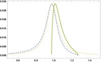
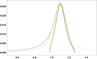
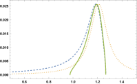
Figure 5: Shape of the pure Breit-Wigner curve (yellow, dotted) vs the production of Breit-Wigner by the phase-space factors of strong decay $Y\to K^{+}K^{-}J\!/\!\psi$ (green, solid) and $Y\to\pi^{+}\pi^{-}J\!/\!\psi$ (blue, dashed) for different resonant effective masses $M_{eff}=$ 990, 1050 and 1100 MeV. All curves are reduced to the same height for better visibility.

By varying the effective mass, we reveal (see in Fig.5) that the maximum of the production of Breit-Wigner and the phase-space factors of strong decay $Y\to K^{+}K^{-}J\!/\!\psi$ is occured at $M_{eff}=1050$ MeV.

We calculate an improved branching ratio in the PSINWA approach as follows:

$$\left[\frac{{\cal B}(Y\!\to\!K^{+}K^{-}J\!/\!\psi)}{{\cal B}(Y\!\to\!\pi^{+}\pi^{-}J\!/\!\psi)}\right]_{PSINWA}=\frac{\Gamma(S\!\to\!K^{+}K^{-})}{\Gamma(S\!\to\!\pi^{+}\pi^{-})}|_{M_{S}=M_{eff}=1050\text{MeV}}\,.$$ (24)

Corresponding numerical result is given in Tab. I.

V.3 Full Integration over resonance momentum

By directly integrating the expression in Eq. (19), we can accurately calculate the branching ratio and obtain the following estimate:

$$\left[\frac{{\cal B}(Y\!\to\!K^{+}K^{-}J\!/\!\psi)}{{\cal B}(Y\!\to\!\pi^{+}\pi^{-}J\!/\!\psi)}\right]_{integ}=\frac{\Gamma(Y\!\to\!K^{+}K^{-}J\!/\!\psi)}{\Gamma(Y\!\to\!\pi^{+}\pi^{-}J\!/\!\psi)}\,.$$ (25)

The related kinematic limits of the decays constrain the integration regions as follows:

$$q^{2}_{max}=(M_{Y}-M_{J\!/\!\psi})^{2}\,,\qquad q^{2}_{min(\pi^{+}\pi^{-})}=4M_{\pi}^{2}\,,\qquad q^{2}_{min(K^{+}K^{-})}=4M_{K}^{2}\,.$$ (26)

VI   Numerical results and Conclusion

The correct determination of the renormalized couplings $g_{H}$ ($H=\{Y,J\!/\!\psi,f_{0},K,\pi\}$) of the participating hadrons is the first step in calculating physical observable decay widths. According to the CCQM, the renormalized couplings are strictly fixed by the compositeness requirements expressed in Eq. (6) and play an important role by excluding the constituent degrees of freedom from the space of physical states.

Using Eqs. (III), (17), (19), (23), (24) and (25) we can determine the partial widths of the strong decays of the $Y$ resonance and their branching ratios after computing the necessary renormalization couplings, $g_{H}$.

The model parameters of the CCQM are determined by minimizing $\chi^{2}$ in a fit to the available experimental data and some lattice results. The fitted parameters may vary around their central value by about $\pm 10\%$, and the errors of our calculations do not exceed also ten percent. The updated central values may be found, e.g., in  Dubnicka:2020 ; Ganbold:2021 . In particular, we have set the charm quark mass and the $J\!/\!\psi$-charmonium size parameter as $m_{c}=1.80$ GeV and $\Lambda_{J\!/\!\psi}\simeq 1.55$ GeV, respectively, in our latest study on the low-lying charmonium states  Ganbold:2021 .

Below, we use the following basic parameter values (in GeV):

 $$\lambda$$          

 0.181  0.264  0.390  1.80  1.25  1.55   .

(27)

We can adjust the size parameters $\Lambda_{\pi}$, $\Lambda_{K}$, $\Lambda_{J\!/\!\psi}$ and $\Lambda_{Y}$ to fit the latest data  PDG2022 ; Ablikim:2022 :

$$\Gamma_{Y}=49\pm 8\text{MeV}\,,\quad\Gamma_{f_{0}}=10\div 100\text{MeV}\,,\quad\left[\frac{{\cal B}(Y\!\to\!K^{+}K^{-}J\!/\!\psi)}{{\cal B}(Y\!\to\!\pi^{+}\pi^{-}J\!/\!\psi)}\right]=0.02\div 0.26\,.$$ (28)

1) The experimental data for the $\Gamma_{f_{0}}=10\div 100\text{MeV}$ is spread too wide, and it can be narrowed by taking the following into account. According to PDG2022 the peak width in $\pi\pi$ is about $50$ MeV, but decay width can be much larger. On the other hand, the branching ratio $\Gamma(f_{0}\to\pi^{+}\pi^{-})/[\Gamma(f_{0}\to\pi^{+}\pi^{-})+\Gamma(f_{0}\to K^{+}K^{-})]$ is about 0.75$\pm$0.13 (see, e.g. PDG2022 ). By assuming that these results are accurate, we can significantly reduce the interval: $60<\Gamma_{f_{0}}<100\text{MeV}$. Further, we will exploit the following average value $\Gamma_{f_{0}}=80\text{MeV}$.

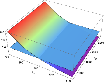
Figure 6: Dependence of the sum $\Gamma(f_{0}\!\to\!K^{+}K^{-})\!+\!\Gamma(f_{0}\!\to\!\pi^{+}\pi^{-})$ on size parameters $\Lambda_{\pi}$ and $\Lambda_{K}$.

2) The size parameters $\Lambda_{\pi}$ and $\Lambda_{K}$ significantly affect the widths of sub-processes $f_{0}\to P^{+}P^{-}$. Particularly, the dependence of the sum $\Gamma(f_{0}\to K^{+}K^{-})+\Gamma(f_{0}\to\pi^{+}\pi^{-})$ expressed in MeV on $\Lambda_{\pi}$ and $\Lambda_{K}$ is shown in Fig. 6. We reveal that the constraint $\Gamma_{f_{0}}<100$ MeV is achieved for the size parameters $\Lambda_{\pi}>900$ MeV and $\Lambda_{K}\sim 1700\div 2200$ MeV.

3) The value of $\Lambda_{Y}$ mostly affects the main decay width values of $Y\to f_{0}J\!/\!\psi$ and $Y\to J\!/\!\psi P^{+}P^{-}$. Corresponding dependence is shown in Fig.7. One can see that the requirements $\Gamma(Y\to f_{0}J\!/\!\psi)<\Gamma_{Y}$ and $\Gamma(Y\!\to\!J\!/\!\psi K^{+}K^{-})\!+\!\Gamma(Y\!\to\!J\!/\!\psi\pi^{+}\pi^{-})<\Gamma_{Y}$ are jointly satisfied for values $\Lambda_{Y}>3550$ MeV.

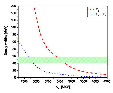
Figure 7: Dependence of the decay widths $\Gamma_{1}=\Gamma(Y\to f_{0}J\!/\!\psi)$ and $\Gamma(Y\!\to\!J\!/\!\psi K^{+}K^{-})\!+\!\Gamma(Y\!\to\!J\!/\!\psi\pi^{+}\pi^{-})$ on size parameter $\Lambda_{Y}$. The green band depicts the data $\Gamma_{Y}=49\pm 8\text{MeV}$  PDG2022 .

In final calculations, we use the optimal values of size parameters as follows:

 $$\Lambda_{\pi}$$    

 0.970 GeV  1.95 GeV  3.75 GeV    .

(29)

We compare the obtained numerical values of the decay widths and branching ratio in Table 1 with the most recent experimental data reported in  PDG2022 and  Ablikim:2022 .

The most recent experimental data reported in  PDG2022 and  Ablikim:2022 are reasonably compatible with our estimates of the Y(4230)-strong decay widths. We observe that the NWA provides rough results that are overly suppressed, whereas its modification, PSINWA, provides more appropriate $Y\!\to\!K^{+}K^{-}J\!/\!\psi$ and $Y\!\to\!\pi^{+}\pi^{-}J\!/\!\psi$ decay widths.

Table 1: Our calculations on the strong decay widths of the charmonium-like state $Y(4230)$ in comparison with the latest data.

Decay	CCQM	PDG2022 PDG2022	BESIII Ablikim:2022
$\Gamma(Y\to J/\psi\,f_{0}$)	6.9 $\pm$ 0.5 MeV	$\Gamma_{Y}$ = 49 $\pm$ 8 MeV	-
$\Gamma(f_{0}\!\to\!K^{+}K^{-})$	3.4 $\pm$ 0.3 MeV	$\Gamma_{f_{0}}$ = 10 $\div$ 100 MeV	-
$\Gamma(f_{0}\!\to\!\pi^{+}\pi^{-})$	75 $\pm$ 6 MeV	$\Gamma_{f_{0}}$ = 10 $\div$ 100 MeV	-
$\Gamma_{NWA}(Y\!\to\!K^{+}K^{-}J\!/\!\psi)$	0.29 $\pm$ 0.03 MeV	$\Gamma_{Y}$ = 49 $\pm$ 8 MeV	-
$\Gamma_{PSINWA}(Y\!\to\!K^{+}K^{-}J\!/\!\psi)$	6.6 $\pm$ 0.5 MeV	$\Gamma_{Y}$ = 49 $\pm$ 8 MeV	-
$\Gamma_{integ}(Y\!\to\!K^{+}K^{-}J\!/\!\psi)$	7.4 $\pm$ 0.6 MeV	$\Gamma_{Y}$ = 49 $\pm$ 8 MeV	-
$\Gamma_{NWA}(Y\!\to\!\pi^{+}\pi^{-}J\!/\!\psi)$	6.5 $\pm$ 0.5 MeV	$\Gamma_{Y}$ = 49 $\pm$ 8 MeV	-
$\Gamma_{PSINWA}(Y\!\to\!\pi^{+}\pi^{-}J\!/\!\psi)$	29.7 $\pm$ 2.5 MeV	$\Gamma_{Y}$ = 49 $\pm$ 8 MeV	-
$\Gamma_{integ}(Y\!\to\!\pi^{+}\pi^{-}J\!/\!\psi)$	31.0 $\pm$ 2.8 MeV	$\Gamma_{Y}$ = 49 $\pm$ 8 MeV	-
$\left[\frac{{\cal B}(Y\!\to\!K^{+}K^{-}J\!/\!\psi)}{{\cal B}(Y\!\to\!\pi^{+}\pi^{-}J\!/\!\psi)}\right]_{NWA}$	0.045 $\pm$ 0.012	-	0.02 $\div$ 0.26
$\left[\frac{{\cal B}(Y\!\to\!K^{+}K^{-}J\!/\!\psi)}{{\cal B}(Y\!\to\!\pi^{+}\pi^{-}J\!/\!\psi)}\right]_{PSINWA}$	0.221 $\pm$ 0.018	-	0.02 $\div$ 0.26
$\left[\frac{{\cal B}(Y\!\to\!K^{+}K^{-}J\!/\!\psi)}{{\cal B}(Y\!\to\!\pi^{+}\pi^{-}J\!/\!\psi)}\right]_{integ}$	0.236 $\pm$ 0.013	-	0.02 $\div$ 0.26

According to our estimate shown in Table I, the decay of the resonance $f_{0}(980)$ into the $K^{+}K^{-}$ pair is more strongly suppressed compared to that into the $\pi^{+}\pi^{-}$ pair, while the branching ratio $|{\cal B}(Y\!\to\!K^{+}K^{-}J\!/\!\psi)/{\cal B}(Y\!\to\!\pi^{+}\pi^{-}J\!/\!\psi)|_{integ}\simeq 0.236$ is near the experimental upper bound reported in  Ablikim:2022 .

We conclude that the estimated branching ratio and calculated fractal strong decay widths of the $Y(4230)$ state do not conflict with the latest experimental data, favoring the molecular representation of the Y-state when the CCQM model is used.

References

(1)
B. Aubert et al. [BaBar Collaboration],
Phys. Rev. Lett. 95, 142001 (2005)
[hep-ex/0506081].
(2)
N. Brambilla et al.,
Eur. Phys. J. C 71, 1534 (2011)
[arXiv:1010.5827 [hep-ph]].
(3)
S. L. Zhu,
Phys. Lett. B 625, 212 (2005)
[hep-ph/0507025].
(4)
E. Kou and O. Pene,
Phys. Lett. B 631, 164 (2005)
[hep-ph/0507119].
(5)
F. E. Close and P. R. Page,
Phys. Lett. B 628, 215 (2005)
[hep-ph/0507199].
(6)
L. Maiani, V. Riquer, F. Piccinini, and A. D. Polosa,
Phys. Rev. D 72, 031502 (2005)
[hep-ph/0507062].
(7)
X. Liu, X. Q. Zeng and X. Q. Li,
Phys. Rev. D 72, 054023 (2005)
[hep-ph/0507177].
(8)
Q. Wang, C. Hanhart, and Q. Zhao,
Phys. Rev. Lett. 111, no. 13, 132003 (2013)
[arXiv:1303.6355 [hep-ph]].
(9)
G. Li and X. H. Liu,
Phys. Rev. D 88, no. 9, 094008 (2013)
[arXiv:1307.2622 [hep-ph]].
(10)
Y. Dong, A. Faessler, T. Gutsche, and V. E. Lyubovitskij,
Phys. Rev. D 89, no. 3, 034018 (2014)
[arXiv:1310.4373 [hep-ph]].
(11)
M. Ablikim et al. [BESIII Collaboration],
Chin. Phys. C, 46,111002 (2022)
[arXiv:2204.07800 [hep-ex]].
(12)
T. Branz, A. Faessler, T. Gutsche, M. A. Ivanov, J. G. Körner, and V. E. Lyubovitskij,
Phys. Rev. D 81, 034010 (2010)
[arXiv:0912.3710 [hep-ph]].
(13)
G. Ganbold, T. Gutsche, M. A. Ivanov, and E. Lyubovitskij,
Phys. Rev. D. 104 094048 (2021)
[arXiv:2107.08774 [hep-ph]].
(14)
S. Dubnička, A. Z. Dubničková, M. A. Ivanov, J. G. Körner,
P. Santorelli and G. G. Saidullaeva,
Phys. Rev. D 84, 014006 (2011)
[arXiv:1104.3974 [hep-ph]].
(15)
F. Goerke, T. Gutsche, M. A. Ivanov, J. G. Körner, V. E. Lyubovitskij,
and P. Santorelli,
Phys. Rev. D 94, no. 9, 094017 (2016)
[arXiv:1608.04656 [hep-ph]].
(16)
F. Goerke, T. Gutsche, M. A. Ivanov, J. G. Körner, and V. E. Lyubovitskij,
Phys. Rev. D 96, no. 5, 054028 (2017)
[arXiv:1707.00539 [hep-ph]].
(17)
M. Ivanov,
EPJ Web Conf. 192, 00042 (2018)
[arXiv:1809.02973 [hep-ph]].
(18)
S. Dubnička, A. Z. Dubničková, A. Issadykov, M. A. Ivanov, and A. Liptaj,
Phys. Rev. D 101, 094030 (2020)
[arXiv:2003.04142 [hep-ph]].
(19)
A. Salam,
Nuovo Cimento 25, 224 (1962).
(20)
S. Weinberg,
Phys. Rev. 130, 776 (1963).
(21)
C. F. Uhlemann and N. Kauer,
Nucl. Phys. B 814 195 (2009).
(22)
R.L. Workman et al. [Particle Data Group],
Prog. Theor. Exp. Phys. 2022, 083C01 (2022).