Abstract

In the context of complex quadratic networks (CQNs) introduced previously, we study escape radius and synchronization properties in two dimensional networks. This establishes the first step towards more general results in higher-dimensional networks.

1 Introduction

In our previous work we have introduced complex quadratic networks (CQNs) as networks of coupled nodes, the dynamics of which is governed by discrete quadratic iterations in the complex plane. As mathematical objects, they have rich and complex behavior, which can exhibit a wide range of phenomena, far transcending those described for single iterated maps. These behaviors are governed by the interplay between the properties of individual nodes, the strength of the coupling between them and the topology of the network, making them a fascinating subject of study in the emerging field of network science. Understanding the effect of edge configuration and weights becomes of crucial interest in the context of understanding and classifying the long-term behavior of the system. In particular, the study of these networks has revealed that even simple changes to the edge weights can lead to large-scale changes in the system’s dynamics. This has significant implications not only for network science, but also for other fields such as physics, biology, and engineering, where understanding the dynamics of complex systems is a critical component.

In order to efficiently quantify the asymptotic dynamics of the system in response to network changes, we defined, for any $n$-dimensional network, an extension of the traditional prisoner set (as the set of bounded initial conditions that have bounded orbits in $\mathbb{C}^{n}$) [4]. We also defined the equi-Mandelbrot set, an extension of the traditional Mandelbrot set, as the set of parameters $c\in\mathbb{C}$ for which the given network with identical nodes $z\to z^{2}+c$ is postcritically bounded in $\mathbb{C}^{n}$). Since the properties of the critical orbit are complicated in this case by the fact that is has multiple components, this definition is not equivalent to the connectedness locus in $\mathbb{C}$ of the network prisoner set, but we conjectured that some relationship remains between the two objects in the parameter plane [2].

In the context of CQNs, one can study a similar concept with that of traditional “synchronization” of nodes’ activity described in the context of networks of continuous-time oscillators. Instead of requiring for two nodes to eventually converge to the same attractor, synchronization of two nodes in CQNs required that the two nodes are simultaneously bounded [1]. To fix ideas, We further defined node-wise equi-Mandelbrot sets as the parameter regions for which individual nodes remain bounded (as the critical orbit evolves in $\mathbb{C}^{n}$). Then we defined two nodes $z_{i}$ and $z_{j}$ to be M-synchronized is they have the same node-wise equi-Mandelbrot sets, i.e., ${\cal M}(z_{i})={\cal M}(z_{j})$. With this relationship, the nodes of a network can be classified into clusters of nodes with identical equi-M sets.

A substantial focus of our work has been on understanding the contribution of the coupling to the topological properties of the equi-M sets, and to the grouping and shapes of the synchronization clusters. In our previous work, we have approached CQNs from a network science standpoint [1, 3], and have focused primarily on the contribution of the network architectural aspect to the emerging dynamics. However, in order to have nontrivial architecture, the network has to be reasonably large. This leap to access higher-dimensional, interesting “connectivity patterns” omitted a specific analyses of two-dimensional networks, which can only have virtually trivial architecture schemes between two nodes.

This case is, nontheless, extremely important in understanding analytically how coupling between two nodes affects the equi-M sets and their synchronization. In this paper we focus precisely on this aspect, and embrace a bottom-up, constructive approach. We show that, by building upon results on interaction between two nodes taken in isolation, one can determine how this type of mutual coupling acts more generally when embedded into higher-dimensional networks.

2 Dynamics of two coupled maps

We consider the system of two coupled complex variables $(z_{1},z_{2})$, evolving discretely according to quadratic complex dynamics $f(z)=z^{2}+c$, $c\in\mathbb{C}$, and with linear coupling specified by the matrix $A=\left(\begin{array}[]{cc}a&b\\ d&f\end{array}\right)$. More precisely, the 2-dimensional map describing the coupled dynamics is given by:

$$z_{1}(n+1) = (az_{1}+bz_{2})^{2}+c$$

$$z_{2}(n+1) = (dz_{1}+fz_{2})^{2}+c$$ (1)

For consistency with our more general prior work in complex quadratic networks (CQNs), we will refer to our two-map coupled systems as 2D-CQNs throughout this paper.

2.1 Escape radius

In this section, we will show that the system of two coupled maps described above has an escape radius, for most connectivity matrices $A$. To do this, we will prove a series of lemma, considering separately different cases for the balance of the connectivity parameters $(a,b,d,f)$.

Lemma 2.1.

Suppose the connectivity matrix $A$ is such that $\Delta=\lvert af\rvert-\lvert bd\rvert\neq 0$. Then there exists a large enough $M>0$ such that, for an iteration step $n\geq 0$ we have $\lvert z_{1}(n)\rvert>M$ or $\lvert z_{2}(n)\rvert>M$, then the next iterates $\lvert z_{1}(n+1)\rvert>2M$ or $\lvert z_{2}(n+1)\rvert>2M$.

Proof.

Since $\Delta=\lvert af\rvert-\lvert bd\rvert\neq 0$, we can consider $\displaystyle\sqrt{K_{1}}=\frac{\lvert b\rvert+\lvert f\rvert}{\lvert\Delta\rvert}$, and $\displaystyle\sqrt{K_{2}}=\frac{\lvert a\rvert+\lvert d\rvert}{\lvert\Delta\rvert}$, and further:

$$M_{1}=K_{1}+\sqrt{K_{1}(K_{1}+\lvert c\rvert)}\text{ and }M_{2}=K_{2}+\sqrt{K_{2}(K_{2}+\lvert c\rvert)}$$

Take $M>\max\{M_{1},M_{2}\}$. Suppose that, for some $n\geq 0$, we have $z_{1}(n)>M$ or $z_{2}(n)>M$. We will show that $z_{1}(n+1)>2M$ or $z_{2}(n+1)>2M$. We will argue by contradiction; throughout the argument, we will abbreviate $z_{1}(n)$ and $z_{2}(n)$ to $z_{1}$ and $z_{2}$, when there is no danger of confusion. Suppose both $z_{1}(n+1)\leq 2M$ and $z_{2}(n+1)\leq 2M$. Then

$$2M\geq\lvert z_{1}(n+1)\rvert=\lvert(az_{1}+bz_{2})^{2}+c\rvert\geq\lvert az_{1}+bz_{2}\rvert^{2}-\lvert c\rvert\geq(\lvert az_{1}\rvert-\lvert bz_{2}\rvert)^{2}-\lvert c\rvert$$

It follows that

$$\lvert\lvert az_{1}\rvert-\lvert bz_{2}\rvert\rvert\leq\sqrt{2M+\lvert c\rvert}$$

Similarly, starting from $\lvert z_{2}(n+1)\rvert\leq 2M$, one can show that:

$$\lvert\lvert dz_{1}\rvert-\lvert fz_{2}\rvert\rvert\leq\sqrt{2M+\lvert c\rvert}$$

Call now $\xi_{1}=\lvert f\rvert(\lvert az_{1}\rvert-\lvert bz_{2}\rvert)$ and $\xi_{2}=\lvert b\rvert(\lvert dz_{1}\rvert-\lvert fz_{2}\rvert)$. Then

$$\lvert\xi_{1}-\xi_{2}\rvert=\lvert(\lvert af\rvert-\lvert bd\rvert)z_{1}\rvert\leq\lvert\xi_{1}\rvert+\lvert\xi_{2}\rvert\leq(\lvert b\rvert+\lvert f\rvert)\sqrt{2M+\lvert c\rvert}$$

hence

$$\lvert z_{1}\rvert\leq\frac{\lvert b\rvert+\lvert f\rvert}{\lvert\Delta\rvert}\sqrt{2M+\lvert c\rvert}$$

From our assumption for $M$ large it follows that the right side of (2.1) is no larger than $M$. Squaring both sides, this is equivalent to $h(M)=M^{2}-K_{1}(2M+\lvert c\rvert)>0$, which is guaranteed by taking $M>M_{1}$, the larger of the quadratic roots of $h$. In conclusion, we obtain that $\lvert z_{1}(n)\rvert\leq M$.

Similarly, if we call $\psi_{1}=\lvert f\rvert(\lvert az_{1}\rvert-\lvert bz_{2}\rvert)$ and $\psi_{2}=\lvert b\rvert(\lvert dz_{1}\rvert-\lvert z_{2}\rvert)$, we get that

$$\lvert\psi_{1}-\psi_{2}\rvert=\lvert(\lvert af\rvert-\lvert bd\rvert)z_{2}\rvert\leq(\lvert a\rvert+\lvert d\rvert)\sqrt{2M+\lvert c\rvert}$$

Hence

$$z_{2}(n)\leq\sqrt{K_{2}}\sqrt{2M+\lvert c\rvert}\leq M$$

(the second part of the double inequality follows from the condition that $M>M_{2}$). Since $z_{1}(n)$ and $z_{2}(n)$ cannot be simultaneously smaller than $M$, the contradiction follows.

∎

We then have the following

Theorem 2.2.

In the case of $\lvert af\rvert\neq\lvert bd\rvert$, $M=\max\{M_{1},M_{2}\}$ acts as an escape radius for the iteration, with $M_{1}$ and $M_{2}$ described in the proof of Lemma 2.1.

Hence, when $\lvert af\rvert\neq\lvert bd\rvert$, $M=\max\{M_{1},M_{2}\}$ acts as an escape radius for the iteration, with $M_{1}$ and $M_{2}$ described in the proof of Lemma 2.1. Suppose now $\lvert af\rvert\neq\lvert bd\rvert$. To fix our ideas, suppose that $af=bd$ (the opposite sign case is similar). We want to see if, in this case, there still exists a large enough $M>0$ such that, for an iteration step $n\geq 0$ we have $\lvert z_{1}(n)\rvert>M$ or $\lvert z_{2}(n)\rvert>M$, then the next iterates $\lvert z_{1}(n+1)\rvert>2M$ or $\lvert z_{2}(n+1)\rvert>2M$. We need to analyze a few distinct cases, as follows:

Case 1: $a,b\neq 0$. Since $af=bd$, we can call $\displaystyle k=\frac{d}{a}=\frac{f}{b}$. Say that, for some fixed iteration $n$, $\lvert z_{1}(n)\rvert>M$ and $\lvert z_{2}\rvert>M$.

Consider $g=\min\{\lvert a\rvert,\lvert b\rvert\}$. It follows that $\lvert az_{1}+bz_{2}\rvert>gM$ or $\lvert az_{1}-bz_{2}\rvert>gM$. Indeed, suppose by contradiction that both $\lvert az_{1}+bz_{2}\rvert\leq gM$ and $\lvert az_{1}-bz_{2}\rvert\leq gM$. Then

$$2\lvert az_{1}\rvert\leq\lvert az_{1}+bz_{2}\rvert+\lvert az_{1}-bz_{2}\rvert\leq 2gM<2\lvert a\rvert M$$

implying that $z_{1}\leq M$. Similarly,

$$2\lvert bz_{1}\rvert\leq\lvert az_{1}+bz_{2}\rvert+\lvert bz_{2}-az_{1}\rvert\leq 2gM<2\lvert b\rvert M$$

implies that $z_{2}\leq M$. Since we cannot have simultaneously $\lvert z_{1}\rvert\leq M$ and $\lvert z_{2}\rvert\leq M$, we get our contradiction.

Suppose $\lvert az_{1}+bz_{2}\rvert>gM$; the case of $\lvert az_{1}-bz_{2}\rvert>gM$ works similarly and we will skip the proof. We consider:

$$az_{1}(n+1)+bz_{2}(n+1)=(a+bk^{2})(az_{1}+bz_{2})^{2}+c(a+b)$$

Hence

$$\lvert az_{1}(n+1)+bz_{2}(n+1)\rvert\geq g^{2}M^{2}\lvert a+bk^{2}\rvert-\lvert c(a+b)\rvert$$

Case (i): If $a+bk^{2}\neq 0$, we can consider the quadratic function $f(M)=g^{2}M^{2}\lvert a+bk^{2}\rvert-2(\lvert a\rvert+\lvert b\rvert)M-\lvert c(a+b)\rvert$. The larger root $M_{1}>0$ of this function is defined explicitly as:

$$M_{1}=\frac{\lvert a\rvert+\lvert b\rvert+\sqrt{(\lvert a\rvert+\lvert b\rvert)^{2}+g^{2}\lvert c\rvert(\lvert a\rvert+\lvert b\rvert)\lvert a+bk^{2}\rvert}}{g^{2}\lvert a+bk^{2}\rvert}$$

If $M>M_{1}$, then $f(M)>0$, and $\lvert az_{1}(n+1)+bz_{2}(n+1)\rvert>2(\lvert a\rvert+\lvert b\rvert)M$. It follows easily that either $\lvert z_{1}(n+1)\rvert>2M$ or $\lvert z_{2}(n+1)\rvert>2M$.

Case (ii): If $a+bk^{2}=0$, then $a=-bk^{2}$, $d=-bk^{3}$ and $f=bk$. Hence the system becomes: $z_{1}(n+1)=b^{2}(-k^{2}z_{1}+z_{2})^{2}+c$ and $z_{2}(n+1)=b^{2}k^{2}(-k^{2}z_{1}+z_{2})^{2}+c$. Call $\xi(n)=-k^{2}z_{1}(n)+z_{2}(n)$. Then one can easily see that $\xi(n)=c(1-k^{2})$ is constant for $n\geq 1$. It follows that $z_{1}(n+1)=b^{2}\xi^{2}(n)+c$ and $z_{2}=b^{2}k^{2}\xi^{2}(n)+c$ are also constant for $n\geq 1$.

Case 2: $a=0$, $b\neq 0$. Then automatically $d=0$, and the system becomes: $z_{1}(n+1)=(bz_{2})^{2}+c$, $z_{2}(n+1)=(fz_{2})^{2}+c$. The second equation is decoupled. If $f\neq 0$, one can make the change of variables $\xi=f^{2}z_{2}$, and rewrite the equation as $\xi(n+1)=\xi^{2}+c_{f}$, where $c_{f}=f^{2}c$. It follows from the traditional theory on escape radius for single quadratic maps that $M=\max\{2/f^{2},\lvert c\rvert\}$ is an escape radius for $z_{2}$. Hence the whole system has an escape radius, since $z_{1}$ only depends on $z_{2}$. It $f=0$, the system is trivial (both $z_{2}$ and $z_{1}$ are constant).

Case 3: $b=0$, $a\neq 0$. Then automatically $f=0$, and the system becomes $z_{1}(n+1)=(az_{1})^{2}+c$, $z_{2}(n+1)=(dz_{1})^{2}+c$. The proof follows similarly with Case 2.

Case 4: $a=b=0$. Then $z_{1}(n)=c$ for all $n\geq 0$ (constant sequence) and $z_{2}(n+1)=(dc+fz_{2})^{2}+c$. Withe the change of variable $\xi=f^{2}z_{2}+dc$, the second equation becomes: $\xi(n+1)=\xi^{2}+c(f^{2}+d)$, which has an escape radius.

Altogether, these cases imply that the escape radius property remains valid when $\lvert af\rvert=\lvert bd\rvert$, as long as $a+bk^{2}\neq 0$. One can easily find singular matrices $A$ (i.e., $af-bd=0$) with $a+bk^{2}=0$, for which the corresponding system does not satisfy the escape radius property. Take for example $a=1$, $b=-1$, $k=1$, in which case $z_{1}(n+1)=z_{2}(n+1)=(z_{2}-z_{1})^{2}+c$. Initial conditions with arbitrarily large $z_{1}(0)=z_{2}(0)$ immediately collapse to $z_{1}(n)=z_{2}(n)=c$, for all $n\geq 1$, showing that there is no radius $M>0$ past which orbits automatically escape to infinity. A different and more difficult question is whether there are networks such that, given any large $M$, there are $c$ values for which the critical orbit can grow larger than $N$, but remain asymptotically bounded. This can inform us if we can have a viable computational test for checking whether a $c$ can be unquestionably excluded from the equi-M set of a given network.

2.2 Synchronization in systems of two coupled maps

In previous work on CQNs, we showed that nodes can independently have different behaviors, with some nodes remaining bounded, while other nodes in the same coupled network escaping asymptotically to infinity.

Lemma 2.3.

If $z_{j}$ has a nontrivial input to $z_{k}$, and if $z_{j}(n)$ is bounded in $\mathbb{C}$ as $n\to\infty$, then $z_{k}(n)$ is also bounded.

Proof.

We can assume without loss of generality that $z_{1}$ is bounded, and that the input $b$ from $z_{2}$ to $z_{1}$ is nonzero, and prove that $z_{2}$ is also bounded. Since $z_{1}$ is bounded, there exists $M>0$ such that $\lvert z_{1}(n)\rvert\leq M$, for all $n\geq 0$. Since $\lvert z_{1}(n+1)\rvert\geq\lvert az_{1}+bz_{2}\rvert^{2}-\lvert c\rvert$, it follows that $\lvert bz_{2}\rvert-\lvert az_{1}\rvert\leq\sqrt{\lvert z_{1}(n+1)\rvert+\lvert c\rvert}$. Then:

$$\lvert bz_{2}\rvert\leq\sqrt{\lvert z_{1}(n+1)\rvert+\lvert c\rvert}+\lvert az_{1}\lvert\leq\sqrt{M+\lvert c\rvert}+\lvert a\rvert M$$

Then, if $b\neq 0$, we have, for all $n\geq 0$:

$$\lvert z_{1}(n)\rvert\leq K=\frac{\leq\sqrt{M+\lvert c\rvert}+\lvert f\rvert M}{\lvert d\rvert}$$

insuring that $z_{2}(n)$ is bounded.

∎

Proposition 2.4.

If $z_{1}$ and $z_{2}$ are nontrivially interconnected (i.e., both $b,d\neq 0$), then they are simultaneously bounded.

In previous work, we have looked in particular at the possible behaviors of the components of the critical orbit of the network, and their “synchronization” into different clusters with identical bounded versus unbounded behavior. More precisely:

Definition 2.5.

For each node $z_{k}$, $1\leq k\leq n$, we define the node-wise equi-M set ${\cal M}_{k}$ as the parameter locus $c\in\mathbb{C}$ for which the component corresponding to the node $z_{k}$ of the critical multi-orbit is bounded. We say that two network nodes $z_{i}$ and $z_{j}$ are M-synchronized, if their equi-M sets ${\cal M}(z_{i})$ and ${\cal M}(z_{j})$ are identical. We also say that the nodes belong to the same M-synchronization cluster (or simply M-cluster) of the network.

In this context, we can reinterpret the results in this sections as

Corollary 2.6.

If in the network described by (1) the nodes $z_{1}$ and $z_{2}$ are nontrivially interconnected (i.e., $b,d\neq 0$), then the nodes are simultaneously bounded. In particular, ${\cal M}(z_{1})={\cal M}(z_{2})$.

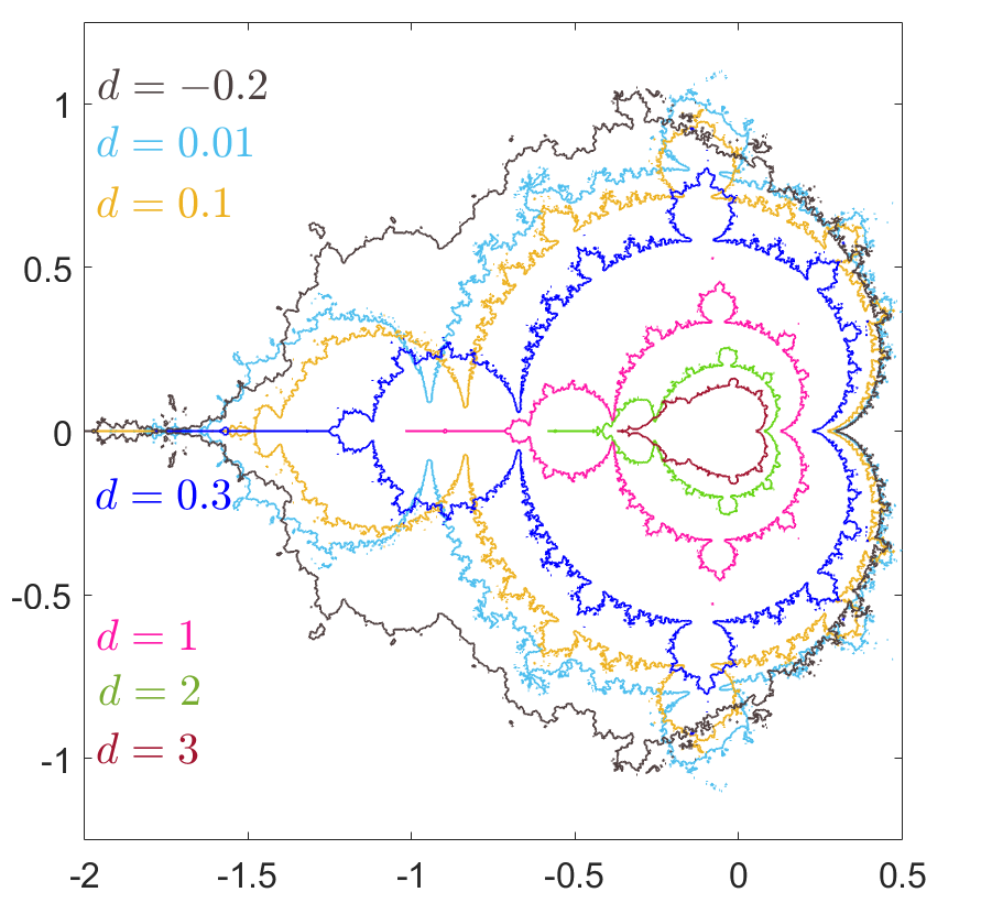
Figure 1: Evolution of the equi M set as the value of $d$ increases. The other entries of the matrix $A$ were fixed to $a=0.6$, $b=0.8$, $f=0.4$. The panel illustrates the equi-M contour (identical between the two nodes), using different colors for different values of $d$, as follows: $d=-0.2$ (grey); $d=0.01$ (cyan); $d=0.1$ (orange); $d=0.3$ (blue, scaling of the traditional Mandelbrot set, since $d$ is the critical values for which $\det(A)=0$); $d=1$ (pink); $d=2$ (green); $d=3$ (brown).

The proof follows directly from Proposition 2.4. Notice that if in addition the matrix $A$ is singular, then $k=\frac{d}{a}=\frac{f}{b}$ and, with the notation $\xi=(a+bk^{2})(az_{1}+bz_{2})$, we have $\xi(n+1)=\xi^{2}+(a+bk^{2})(a+b)c$. The values of $c$ for which $z_{1}$ and $z_{2}$ are (simultaneously) bounded are the same as the values of $c$ for which $(a+bk^{2})(a+b)c$ is in the traditional Mandelbrot set. Hence the equi M set (identical between the two nodes) is in this case a rescaling of the traditional set. Figure 1 illustrates how the shape of the equi M set of the two synchronized nodes evolves as the value of $d$ increases through the negative and positive range as the other three entries of $A$ are fixed, crossing through the critical value which makes $A$ singular. Notice that, as $d$ is increasing from negative values, the shape slowly approaches that of the traditional Mandelbrot set (achieved for the critical $d=0.3$), and then slowly degrades away from this shape as $d$ continues to increase.

This sheds some light on the effects of the coupling when the nodes are interconnected ($b,d\neq 0$). At the other end of the spectrum, we have the case when the nodes both act independently. This case is trivial, as described in the following lemma:

Lemma 2.7.

If $b=d=0$ and $a,f\neq 0$, then the two node-wise equi M sets are both scaled versions of the traditional Mandelbrot set.

Proof.

We have $z_{1}(n+1)=(az_{1})^{2}+c$, and $z_{2}(n+1)=(fz_{2})^{2}+c$. Then $c\in{\cal M}(z_{1})\Longleftrightarrow ac\in{\cal M}\Longleftrightarrow{\cal M}(z_{1})=\frac{1}{a^{2}}{\cal M}$. Similarly, ${\cal M}(z_{2})=\frac{1}{f^{2}}{\cal M}$. ∎

A natural question to ask next is whether the nodes need to necessarily be nontrivially interconnected in order to be M-synchronized. The answer to that is negative. The following lemma gives a weaker condition that insures M-synchronization of the two nodes (although it does not deliver the stronger result in Corollary 2.4).

Lemma 2.8.

Suppose $z_{1}(n+1)=(az_{1})^{2}+c$ (decoupled), and $z_{2}(n+1)=(dz_{1}+fz_{2})^{2}+c$. Then, for $\lvert f\rvert$ sufficiently small, if the $z_{1}$ component of the critical orbit is bounded, then the $z_{2}$ component is also bounded.

Proof.

Since $z_{1}$ is bounded, there exists a large enough $M>0$ such that $z_{1}(n)\leq M$, for all $n\geq 0$. (Note: the value of $M$ depends on $a$ and $\lvert c\rvert$.) Assume $\lvert f\rvert$ is small enough so that

$$4M\lvert fd\rvert+4\lvert f\rvert^{2}\lvert c\rvert<1$$ (2)

Then the discriminant of the quadratic function in $X$

$$h(X)=\lvert f\rvert^{2}X^{2}+(2M\lvert df\rvert-1)X+M^{2}\lvert d\rvert^{2}+\lvert c\rvert$$

is $\Delta=1-4M\lvert fd\rvert-4\lvert f\rvert^{2}\lvert c\rvert>0$. If we call $X_{1}<X_{2}$ the two distinct roots of $h(X)=0$, then the larger root $X_{2}$is positive. Consider $\max\{X_{1},0\}<K<X_{2}$. Clearly, we have that $h(K)<0$. We will show inductively that $K$ is an upper bound for $z_{2}(n)$, for all $n\geq 0$. Indeed, $z_{2}(0)=0<K$. Now suppose $\lvert z_{2}\rvert=\lvert z_{2}(n)\rvert<K$, and consider

$$\lvert z_{2}(n+1)\rvert = \lvert(dz_{1}+fz_{2})^{2}+c\rvert\leq\lvert dz_{1}+fz_{2}\rvert^{2}+\lvert c\rvert\leq(\lvert d\rvert M+\lvert fz_{2}\rvert)^{2}+\lvert c\rvert$$ (3)

$$= \lvert d\rvert^{2}M^{2}+2\lvert fd\rvert M\lvert z_{2}\rvert+\lvert f\rvert^{2}\lvert z_{2}\rvert^{2}+\lvert c\rvert\leq\lvert d\rvert^{2}M^{2}+2\lvert fd\rvert MK+\lvert f\rvert^{2}K^{2}+\lvert c\rvert$$

$$= h(K)+K<K$$

Hence $\lvert z_{2}(n+1)\rvert<K$, and the induction is complete. In conclusion, $K$ is an upper bound for the critical component $z_{2}$.
∎

Corollary 2.9.

If $z_{1}(n+1)=(az_{1})^{2}+c$, and $z_{2}(n+1)=(dz_{1}+fz_{2})^{2}+c$, with $a,d\neq 0$ and $\lvert f\rvert$ sufficiently small, then ${\cal M}(z_{1})={\cal M}(z_{2})$.

Proof.

Follows easily from Lemmas 2.3 and 2.8. ∎

Remark. Corollary 2.9 states that, if node $z_{2}$ depends on $z_{1}$, but $z_{1}$ does not depend on $z_{2}$, then a sufficiently weak self-dependence of $z_{2}$ will still insure M-synchronization. What weak means in this context, and how this bound depends on the other system parameters will become obvious in the proof of the lemma.

Figure 2 illustrates the behavior of the equi M contours for positive values of $f$, as $\lvert f\rvert$ decreases, when the first node is decoupled ($b=0$), for different fixed values of $a\neq 0$ and $d\neq 0$. Notice that the nodes eventually synchronize in each case for small enough values of $\lvert f\rvert$. In addition, as expected from the proof of Corollary 2.9, the threshold depends on the values of $a$ and $d$.

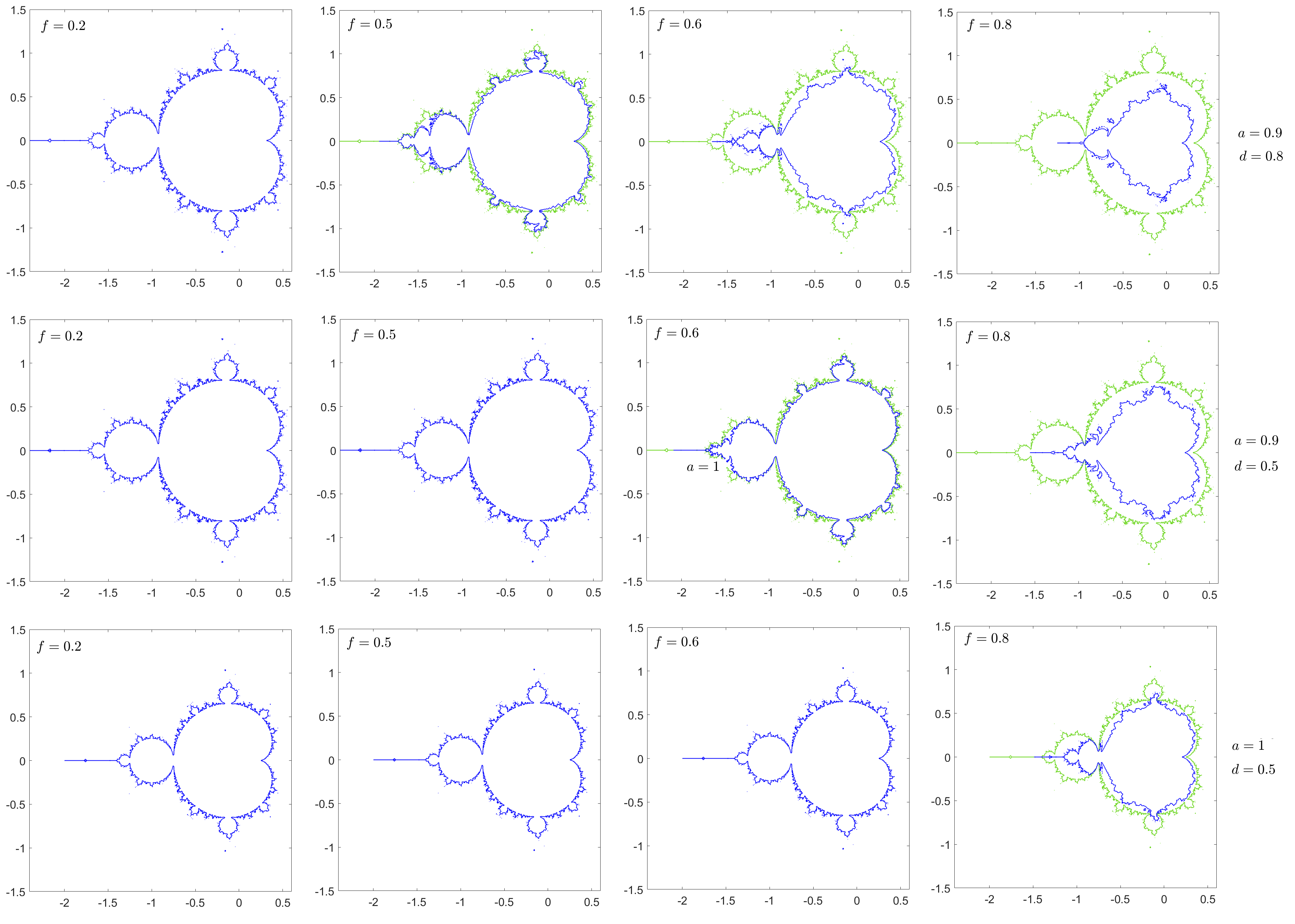
Figure 2: Equi-M Evolution of M synchrinization in a 2D CQN when changing $f$. Each panel shows the two contours of the node-wise equi M sets, in green (for $z_{1}$) and in blue (for $z_{2}$). Top-down, the panels illustrate, respectively:.

In future work, we are interested to investigate necessary and sufficient conditions under which this result can be extended to larger size networks.

References

• [1] Anca Radulescu, Danae Evans, Amani-Daisa Augustin, Anthony Cooper, Johan Nakuci, and Sarah Muldoon. Synchronization and clustering in complex quadratic networks. arXiv:2205.02390, 2022.
• [2] Anca Rǎdulescu and Simone Evans. Asymptotic sets in networks of coupled quadratic nodes. Journal of Complex Networks, 7(3):315–345, 2019.
• [3] Anca Radulescu, Johan Nakuci, Simone Evans, and Sarah Muldoon. Computing brain networks with complex dynamics. arXiv:2209.05268, 2022.
• [4] Anca Rǎdulescu and Ariel Pignatelli. Real and complex behavior for networks of coupled logistic maps. Nonlinear Dynamics, 87(2):1295–1313, 2017.