Depth Super-Resolution from Explicit and Implicit High-Frequency Features

Abstract

Guided depth super-resolution aims at using a low-resolution depth map and an associated high-resolution RGB image to recover a high-resolution depth map. However, restoring precise and sharp edges near depth discontinuities and fine structures is still challenging for state-of-the-art methods. To alleviate this issue, we propose a novel multi-stage depth super-resolution network, which progressively reconstructs HR depth maps from explicit and implicit high-frequency information. We introduce an efficient transformer to obtain explicit high-frequency information. The shape bias and global context of the transformer allow our model to focus on high-frequency details between objects, i.e., depth discontinuities, rather than texture within objects. Furthermore, we project the input color images into the frequency domain for additional implicit high-frequency cues extraction. Finally, to incorporate the structural details, we develop a fusion strategy that combines depth features and high-frequency information in the multi-stage-scale framework. Exhaustive experiments on the main benchmarks show that our approach establishes a new state-of-the-art.

This paper is under consideration at Computer Vision and Image Understanding.

1 Introduction

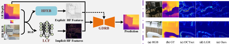
Fig. 1: Depth Super-Resolution exploiting explicit and implicit high-frequency features. On the left, an overview of our framework, combining the power of both explicit and implicit high-frequency information extracted from the inputs. On the right, qualitative examples with (a) RGB images, (b) ground truth depth and error maps by existing methods (c – d) and ours (e).

With the rise of consumer-grade depth cameras, depth maps are employed in various scenarios such as 3D reconstruction (Chen et al., 2020a, b), recognition (Cai et al., 2010) and more. Time-of-Flight (ToF) is one of the leading technologies involved in depth sensing, measuring the distance traveled by emitted rays until they reach points in the scenes. However, due to the limitations of physical fabrication, power consumption and costs (Bamji et al., 2022), the resolution of depth maps usually is often insufficient to fulfill the demand of the downstream applications, such as object detection (Chen et al., 2021) and pose estimation (Ge et al., 2019). In contrast, collecting RGB images at much higher resolution is cheaper. As a result, the guided depth super-resolution task, known as GDSR, has emerged as a crucial solution to this technological limitation, allowing to obtain an accurate high-resolution (HR) depth map from a low-resolution (LR) one, guided by an HR image.

Initially, algorithms addressing this problem were classified into local (Kopf et al., 2007; Yang et al., 2007; Riemens et al., 2009; Wang et al., 2014) and global (Diebel and Thrun, 2005; Park et al., 2011; Ferstl et al., 2013; Li et al., 2016b), with the former family being faster, yet suffering in low-textured regions and the latter resulting more robust, at the expense of processing time. More recently, deep neural networks have become the preferred choice for depth super-resolution (Hui et al., 2016; Li et al., 2016a, 2019; Lutio et al., 2019; Tang et al., 2021b), although they still struggle to restore sharp and precise edges from LR depth maps reliably, especially when dealing with large upsampling factors. This is mainly due to the inadequate guidance provided by High-Frequency (HF) features, implicitly modeled by deep networks, which frequently cause texture copying effects in the upsampled depth maps. In addition, single-stage multi-scale architectures for this task (Ye et al., 2020; Wang et al., 2020; Zuo et al., 2020; Tang et al., 2021a), at any given scale, cannot fully leverage fine details encoded at the higher ones, as they are lost due to down-sampling and only partially recovered through skip connections.

In light of the two weaknesses highlighted so far, we aim to improve GDSR by explicitly countering them. For the former, we argue that explicit extraction of HF features, supported by edge detection algorithms such as the Canny operator, can play a crucial role (Wang et al., 2020). Concerning the latter, multi-stage network design – which outperforms single-stage counterparts in high-level visual tasks like action segmentation (Farha and Gall, 2019) and pose estimation (Chen et al., 2018), as well as for low-level vision problems such as image restoration (Zamir et al., 2021; Kim et al., 2022) – can mitigate the information loss issue. However, since features extracted from RGB images need to be considered in addition to depth features, existing multi-stage networks are inadequate for GDSR and should be revised to fuse features from the two domains.

In this paper, we present a Depth Super-Resolution method leveraging both Explicit and Implicit HF information (DSR-EI), which contains two branches: the High-Frequency Extraction Branch (HFEB) and the Guided Depth Restoration Branch (GDRB). The former is designed to model explicit HF features by exploiting dynamic self-calibrated convolutions (DSP) and the power of vision transformers blocks. The latter effectively fuses the guidance from RGB features with depth features to obtain HR depth maps. This is achieved by deploying two novel modules: 1) the Adaptive Feature Fusion Module (AFFM), which counters the HF information loss due to downsampling, and 2) the Low-Cut Filtering (LCF) module, which acts in the frequency domain to improve implicit extraction of HF features. Exhaustive experiments on several standard datasets show the superiority of DSR-EI. In summary, the main contributions of this paper are:

• The proposed architecture employs a novel efficient transformer for explicit, HF feature extraction. The transformer can accurately capture image details and structures from depth maps.

• In the guided depth restoration branch, we propose a low-cut filtering module that can obtain accurate, implicit HF information.

• To counter the information loss issue, we propose an Adaptive Feature Fusion Module located in the middle of the guided depth restoration branch.

• Quantitative and qualitative experimental results demonstrate that our approach establishes a new state-of-the-art in the field of guided depth super-resolution.

Fig. 1 provides a high-level view of our framework, followed by examples that anticipate the superior accuracy achieved by DSR-EI compared to existing methods (Zhao et al., 2022; de Lutio et al., 2022). In case of acceptance, we will make our code publicly available to ease reproducibility.

2 Related Work

In this section, we first review the literature related to the GDSR task, divided into conventional and learning methods, as well as to vision transformers.

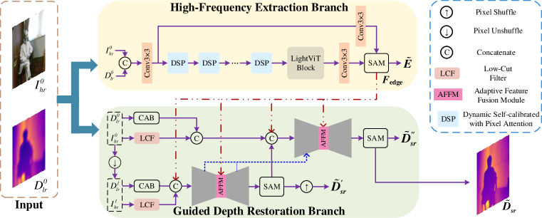
Fig. 2: DSR-EI architecture. Rectangles with different colors depict different stages and functions in each stage.

Conventional Methods. Initially, hand-craft models were developed for GDSR, using the edge co-occurrence between the LR depth map and its HR color counterpart as prior. Kopf et al. (2007) first utilizes a joint bilateral filter, taking guidance cues from color images. The so-called local methods followed this pivotal work: Yang et al. (2007) enhances the LR depth maps by exploiting registered HR color images, Riemens et al. (2009) uses anti-alias image prefiltering built on the multi-stage joint bilateral filter, while graph-based joint bilateral upsampling (Wang et al., 2014) casts GDSR as a regularization problem.

More accurate solutions, although slower, are represented by global methods. The first work in this direction is Diebel and Thrun (2005), which employs Markov random fields (MRF) to integrate multi-modal data for LR depth map upsampling. Using the non-local mean filtering method, Park et al. (2011) recovers noisy LR images from a ToF camera to a high-quality image. To be more efficient, Ferstl et al. (2013) exploits Total Generalized Variation (TGV) regularization for GDSR, enabling a high frame rate. Li et al. (2016b) uses fast global smoothing (FGS) to make guided depth interpolation more robust.

Learning Methods. Earlier methods from this category exploit MRF (Mac Aodha et al., 2012; Kiechle et al., 2013; Kwon et al., 2015). However, these techniques rely on manually created dictionaries, whose limited content restricts the capacity of generalizing. More recently, deep learning-based approaches achieved remarkable results and became the preferred choice for GDSR. Hui et al. (2016) designs a multi-scale guided CNN using hierarchical feature extraction to gradually restores blurred edges. To reconstruct sharp edges, the works by Li et al. (2016a, 2019) learn salient features from color images using an encoder-decoder structure. In contrast, Lutio et al. (2019) casts GDSR as a pixel-to-pixel mapping from the HR RGB image to the domain of the LR source image, learned by a multi-layer perceptron. In Ye et al. (2020), a multi-branch network with progressive refinement performs adaptive information fusion to restore depth details. Wang et al. (2020) can quickly upsample depth maps by learning Canny edges, while Zuo et al. (2020) proposes a depth-guided affine transformation where the feature refinement is carried out iteratively. Tang et al. (2021a) makes use of implicit neural interpolation, Kim et al. (2021) develops a deformable kernel network whose outputs are per-pixel kernels, and Zhao et al. (2022) proposes a Discrete Cosine Transform Network (DCTNet) to extract multi-modal features effectively. Through graph optimization, de Lutio et al. (2022) combines the advantages of model-driven and deep learning-based methods. Concurrent works exploit recurrent structure attention (Yuan et al., 2023) or combine deep learning with anisotropic diffusion (Metzger et al., 2022).

Despite substantial advancements, these networks are not effective enough at extracting HF guidance from RGB images. Inspired by Liu et al. (2021), this paper tackles GDSR leveraging both explicit and implicit HF features guidance.

Vision Transformers. Transformers, initially designed for natural language processing (Vaswani et al., 2017), recently gained popularity in computer vision, for tasks such as image recognition (Dosovitskiy et al., 2021; Touvron et al., 2021), object detection (Carion et al., 2020) and semantic segmentation (Wang et al., 2021). Vision Transformers (ViTs) learn long-range dependencies across image tokens through self-attention (Han et al., 2022). Given the natural advantages of such a mechanism, ViTs targeting low-level vision tasks emerged more recently (Zamir et al., 2022; Lee et al., 2022; Pu et al., 2022), although requiring much larger amounts of parameters and computing resources.

3 DSR-EI Framework

In GDSR, HF information in color images – complementary to depth maps – is essential for achieving high performance, which motivates us to seek an efficient method to extract it. In this section, we present our framework that exploits explicit and implicit HF information for depth super-resolution. Then, we introduce the two branches in our network: the High-Frequency Extraction Branch (HFEB) and the Guided Depth Restoration Branch (GDRB).

(a)

Fig. 3: High-frequency information loss (factor $4\times$). From left to right, HR depth map and its corresponding gradient map, followed by the gradient map from bicubic upsampled LR depth map and LR depth map itself. HF information is mostly lost in the second gradient map.

Fig. 2 shows an overview of our architecture. Given the LR depth map $D_{lr}\in\mathbb{R}^{h\times w\times 1}$ and the corresponding HR color image $I_{hr}\in\mathbb{R}^{H\times W\times 3}$, we aim at restoring HR depth map $\tilde{D}_{sr}$. Note that $H=s\times h$ and $W=s\times w$, where $s$ denotes the upsampling factor – e.g., $4\times,8\times$ or even $16\times$. In our proposed network, the input depth map is firstly upsampled with bicubic interpolation to the same size as $I_{hr}$. At different scales, we denote the corresponding depth maps and color images as $D_{lr}^{i}$ and $I_{hr}^{i}$, respectively, with $s=2^{i}$. Then, according to the above notation, the input images $D_{lr}^{0}$ and $I_{hr}^{0}$ are fed into the two branches, respectively. Before being sent to GDRB, both the RGB and depth images are processed by a channel-attention block (CAB) (Zhang et al., 2018) and a low-cut filtering (LCF) module, which will be explained in detail in Sec. 3.2.

3.1 High-Frequency Extraction Branch (HFEB)

We argue HF information is crucial for effective super-solving depth and is often lost by upsampling. The primary goal of HFEB is to produce an accurate gradient map from an LR depth map, with the support of a color image jointly processed with it.

Indeed, as pointed out in Wang et al. (2020), networks for GDSR tend to focus more on depth discontinuities or object boundaries. However, from Fig. 3, we can notice that even with a $4\times$ factor, most high-frequency information vanishes, as shown by the gradient maps extracted from HR and upsampled LR depth maps, leading to severe degradation of the super-solved depth map. Traditional methods tend to transfer texture to depth maps rather than structural details, failing to extract accurate edges. Moreover, methods extracting binary edges (Wang et al., 2020) gather insufficient high-frequency information, yielding sub-optimal results.

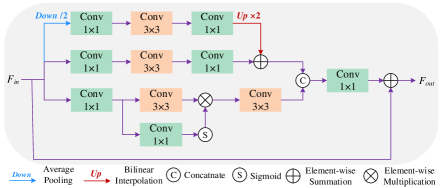
(a)

Fig. 4: DSP architecture. Differently from SCPA (Zhao et al., 2020), our module processes features at different scales, allowing to extract explicit HF information more effectively.

The work (Pu et al., 2022) has shown that transformer-based networks can extract clear and meaningful edges by leveraging both global and local features simultaneously. Considering the sparsity of edge maps, we design an efficient transformer, inspired by dynamic scale policy (Wang et al., 2019) and self-attention (Vaswani et al., 2017), to obtain strong HF priors for guiding depth super-resolution. Specifically, our transformer consists of a stack of blocks called dynamic self-calibrated convolution with pixel attention (DSP) and one LightViT block (Huang et al., 2022). To better extract HF features, we design the DSP block, which is inspired by SCPA (Zhao et al., 2020) and performs self-calibrated convolution with two branches at a single scale. However, unlike SCPA, our DSP block includes an additional branch that enables the processing of features at different scales without incurring extra computational burden, as we will demonstrate empirically in our experiments. Specifically, stacked DSP blocks can be expressed as:

$$\Phi_{M}=\mathcal{F}_{DSP}^{M}(\mathcal{F}_{DSP}^{M-1}(\cdot\cdot\cdot\mathcal{F}_{DSP}^{1}(\Phi_{0})\cdot\cdot\cdot))$$ (1)

where $\mathcal{F}_{DSP}^{m}$ denotes the mapping of the $m$-th DSP block, $m\in[1,M]$, $\Phi_{0}$ and $\Phi_{M}$ are the input/output features, respectively. As shown in Fig. 4, each DSP block includes three branches: the upper is the dynamic scale branch, the middle is the flat convolution branch, and the lower is the pixel attention branch. Specifically, we employ three convolutions with $1\times 1$ kernel to split the channels, which are further processed by each branch. Note that the dynamic scale branch needs to be downsampled before $1\times 1$ convolution. Given the input $\Phi_{m-1}$, we obtain:

$$\Phi_{m-1}^{1}=Conv_{1\times 1}((\Phi_{m-1})\downarrow)$$ (2)

$$\Phi_{m-1}^{k}=Conv_{1\times 1}(\Phi_{m-1})$$ (3)

where $\Phi_{m-1}^{1}$ is the output from the upper dynamic scale branch, $k=2,3$ denotes the features of the other two branches, $Conv_{1\times 1}$ is $1\times 1$ convolution, and $\downarrow$ is the downsampling operation. Except for the pixel attention branch, which has features with half the total channels, the other two branches process features with $\frac{1}{4}$ of the channels each. Next, the pixel attention branch obtains features through the pixel attention scheme (Zhao et al., 2020). In contrast, the other two branches extract spatial information with a $3\times 3$ flat convolution, followed by a $1\times 1$ convolution to restore the number of channels to be the same as the pixel attention branch. Note that the dynamic scale branch needs upsampling after $1\times 1$ convolution. Then, the features from the dynamic scale and the flat convolution branches can be fused by summation. After concatenation of the features followed by a $1\times 1$ convolution, the DSP finally generates the output features $\Phi_{m}$ in a residual learning fashion. It can be written as follows:

$$\Phi_{m}^{1}=Conv_{1\times 1}(Conv_{3\times 3}(\Phi_{m-1}^{1}))\uparrow$$ (4)

$$\Phi_{m}^{2}=Conv_{1\times 1}(Conv_{3\times 3}(\Phi_{m-1}^{2}))$$ (5)

$$\Phi_{m}^{3}=Conv_{3\times 3}(\Phi_{m-1}^{3})\odot\sigma(Conv_{1\times 1}(\Phi_{m-1}^{3}))$$ (6)

$$\Phi_{m}^{{}^{\prime}}=Conv_{3\times 3}(\Phi_{m}^{3})$$ (7)

$$\Phi_{m}^{{}^{\prime\prime}}=Conv_{3\times 3}(\Phi_{m}^{1}\oplus\Phi_{m}^{2})$$ (8)

where $\sigma$ is the sigmoid function, $\odot$ and $\oplus$ are element-wise multiplication and element-wise summation, respectively, and $\uparrow$ denotes the upsampling operation. After concatenation of the features $\Phi_{m}^{{}^{\prime}}$ and $\Phi_{m}^{{}^{\prime\prime}}$ followed by a $1\times 1$ convolution, the DSP finally generates the output features $\Phi_{m}$ in a residual learning manner. This process can be expressed as follows:

$$\Phi_{m}=Conv_{1\times 1}([\Phi_{m}^{{}^{\prime}},\Phi_{m}^{{}^{\prime\prime}}])\oplus\Phi_{m-1}$$ (9)

where $[\cdot]$ perform concatenation.

To further enhance the feature representation of the subnetwork, we incorporate LightViT (Huang et al., 2022) as the tail module, which utilizes local-global attention broadcast to aggregate information from all tokens, allowing for the efficient integration of global dependencies of local tokens into each image token. Finally, considering that the supervised attention module (SAM) (Zamir et al., 2021) can restore information progressively between stages/branches, we employ it to output the gradient map $E\in\mathbb{R}^{H\times W\times 1}$ and high-frequency features $F_{edge}\in\mathbb{R}^{H\times W\times C}$, used respectively as intermediate output – allowing for explicit supervision over edges – and as guidance for GDRB. Under this lightweight design, HFEB can effectively still extract meaningful structural information with different scale receptive fields.

3.2 Guided Depth Restoration Branch (GDRB)

As shown in Fig. 2, GDRB is composed of two stages, and each one processes features at three scales, following a coarse-to-fine strategy (Gao et al., 2019; Sarlin et al., 2019). The two stages are implemented with standard U-net architectures (Ronneberger et al., 2015). More specifically, a cross-stage feature fusion module (Zamir et al., 2021) is deployed between the two, which proved to be effective in image restoration and, in our design, allows GDRB to benefit from the intermediate features extracted by HFEB. To prevent aliasing in downsampling, we employ content-aware filtering layers (Zou et al., 2022) in the encoders. Besides, GDRB deploys some further SAM blocks (Zamir et al., 2021), allowing valuable features to propagate to the next stage. In addition to depth features, the SAMs of the two stages also output depth maps $\tilde{D}_{sr}^{{}^{\prime}}$ and $\tilde{D}_{sr}^{{}^{\prime\prime}}$, to which intermediate supervision is provided. Note that input images are downsampled to the lower stage using pixel unshuffling to prevent information loss. Subsequently, the depth map output of this stage is restored at high resolution by employing pixel shuffling.

Based on the above structure, we propose two novel modules: AFFM and LCF. The former fuses gradient features between each encoder/decoder, while the latter supplements additional HF information in an implicit manner.

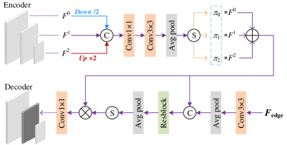
(a)

Fig. 5: AFFM architecture, operating at middle scale. AFFMs for the remaining scales follow the same design.

Adaptive feature fusion module. Recent networks such as Ye et al. (2020); Tang et al. (2021a) typically concatenate RGB and depth features directly during feature fusion, followed by additional operations such as channel attention (Zhang et al., 2018) to capture useful information. In contrast, inspired by Liu et al. (2021), we run adaptive feature fusion through AFFM in two steps to strengthen the reconstruction of HF cues, as illustrated in Fig. 5. We differentiate from Liu et al. (2021) by using dynamic convolution (Chen et al., 2020c) to better aggregate depth and HR features. In the first step, we generate dynamic weights $\pi_{i},i=0,1,2$, which are then assigned to features from different scales within the current stage. Finally, we perform element-wise summation to obtain the feature maps $F^{{}^{\prime}}$. For clarity, the figure shows the module working at the middle scale of the network as an example, with the others sharing the same design. The process is defined as follows:

$$F_{cat}=Conv_{3\times 3}(Conv_{1\times 1}([F^{0}\downarrow,F^{1},F^{2}\uparrow]))$$ (10)

$$\{\pi_{0},\pi_{1},\pi_{2}\}=\sigma(Avgpool(F_{cat}))$$ (11)

$$F^{{}^{\prime}}=\pi_{0}\cdot F^{0}\downarrow+\pi_{1}\cdot F^{1}+\pi_{2}\cdot F^{2}\uparrow$$ (12)

where $F^{i},i=0,1,2$ denotes the feature maps from the three scales, and $\downarrow$, $\uparrow$ are respectively downsampling and upsampling operators.

In the second step, gradient features $F_{edge}$ from HFEB are concatenated with $F^{{}^{\prime}}$. Then, per-pixel attention maps $F_{att}$ are generated by a ResBlock (He et al., 2016) followed by an average pooling operation. These attention maps are then applied directly to the adaptively fused features $F^{{}^{\prime}}$ through element-wise multiplication operation. Finally, after $1\times 1$ convolution, the attention-guided features $F_{out}^{i}$ are delivered to the corresponding scale of the current stage. In Fig. 5, the output is passed to the middle scale of the decoder. AFFMs working at the other scales send their output to the corresponding scale in the decoder. This step can be formalized as follows:

$$F^{{}^{\prime\prime}}=[Avgpool(Conv_{3\times 3}(F_{edge})),F^{{}^{\prime}}]$$ (13)

$$F_{att}=\sigma(Avgpool(ResBlock(F^{{}^{\prime\prime}})))$$ (14)

$$F_{out}^{1}=con_{1\times 1}(F^{{}^{\prime}}\otimes F_{att})$$ (15)

where $\otimes$ is an element-wise multiplication operation and $F_{out}^{1}$ denotes the output features at the middle scale.

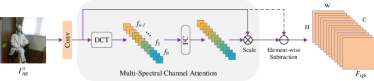
Fig. 6: Low-cut filtering module (LCF). LF features are extracted through DCT and multi-spectral channel attention, and subtracted from the input to retain HF features.

Low-cut filtering module. The performance of our method greatly benefits from the explicit gradient information, but some valuable high-frequency information still vanishes. This fact motivates us to consider extracting complementary information in the frequency domain. As a common practice (Chang et al., 2007; Lin et al., 2010), we use the low-frequency information of the discrete cosine transform (DCT) to compress images. Based on the design approach proposed in Qin et al. (2021), we develop a filtering module utilizing feature decomposition in the frequency domain to extract low-frequency components from the input. Specifically, we apply a $1\times 1$ convolution followed by a channel split to the input color image $I_{hr}^{0}$. Then, we can obtain assigned frequency components from the output features $[{f}_{0},{f}_{1},\cdot\cdot\cdot,{f}_{n-1}]$ after DCT. Thus, the multi-spectral channel attention maps are generated by a fully connected layer and sigmoid activation. According to Qin et al. (2021), the low-frequency information is first assured to pass. Thus, we subtract such a low-frequency component from the input features producing the complementary high-frequency features $F_{rgb}$. Fig. 6 illustrates LCF in detail. The high-frequency cues extracted from these features enable GDRB to progressively super-resolve LR depth maps into HR ones.

Refinement. To enhance the depth quality further, we optionally feed our final output into NLSPN (Park et al., 2020) for refinement. This variant of the method is referred to as DSR-EI⁺.

3.3 Training Loss

Our network is trained in an end-to-end fashion using two loss terms: depth loss $L_{d}$ and gradient loss $L_{g}$. The depth loss is defined as:

$$L_{d}\!=\!\parallel\!(\!\tilde{D}_{sr}\!-\!D_{gt})\!\odot\!\mathbb{I}\!\parallel_{1} +\lambda_{d}\cdot\!\parallel\!(\!\tilde{D}_{sr}^{{}^{\prime}}\!-\!D_{gt})\!\odot\!\mathbb{I}\!\parallel_{1}\!$$ (16)

$$+\lambda_{d}\cdot\!\parallel\!(\!\tilde{D}_{sr}^{{}^{\prime\prime}}\!-\!D_{gt})\!\odot\!\mathbb{I}\!\parallel_{1}$$

where $D_{gt}$ is the ground truth depth, $\tilde{D}_{sr}$, $\tilde{D}_{sr}^{{}^{\prime}}$ and $\tilde{D}_{sr}^{{}^{\prime\prime}}$ are predicted depth maps from different stages, and $\mathbb{I}$ is pixel validity, as defined in de Lutio et al. (2022). We empirically set $\lambda_{d}=0.2$. Gradient loss $L_{g}$ is computed on HEFB output, as:

$$L_{g}=\parallel\tilde{E}-E_{gt}\parallel_{1}$$ (17)

where $\tilde{E}$ is the predicted gradient map and $E_{gt}$ is the ground truth one, extracted according to Liu et al. (2021). Thus, the total loss can be defined as:

$$L_{total}=L_{d}+\lambda_{g}\cdot L_{g}$$ (18)

with $\lambda_{g}$ empirically set to 0.01.

Table 1: Results on Middlebury, NYUv2 and DIML datasets. The lower the MSE and MAE, the better.

Dataset	Middlebury			NYUv2			DIML
Methods	$4\times$	$8\times$	$16\times$	$4\times$	$8\times$	$16\times$	$4\times$	$8\times$	$16\times$
GF (He et al., 2010)	33.3 / 1.27	40.5 / 1.49	67.4 / 2.21	114 / 3.91	142 / 4.47	249 / 6.34	25.6 / 1.45	34.1 / 1.77	66.3 / 2.74
SD (Ham et al., 2017)	24.9 / 0.46	82.5 / 0.86	511 / 1.73	36.0 / 1.31	105 / 2.57	533 / 5.07	10.5 / 0.40	44.9 / 0.83	41.1 / 1.91
P2P (Lutio et al., 2019)	39.8 / 0.79	32.7 / 0.82	41.5 / 1.24	112 / 3.61	122 / 3.86	219 / 5.40	20.7 / 1.15	23.0 / 1.26	39.3 / 1.78
MSG (Hui et al., 2016)	4.13 / 0.22	10.5 / 0.43	34.2 / 1.06	6.85 / 0.81	24.1 / 1.66	84.5 / 3.35	1.73 / 0.22	4.13 / 0.40	13.0 / 0.93
DKN (Kim et al., 2021)	4.29 / 0.18	11.2 / 0.38	47.6 / 1.42	11.4 / 1.03	29.8 / 1.82	115 / 4.01	3.47 / 0.33	5.47 / 0.45	19.3 / 1.20
FDKN (Kim et al., 2021)	3.60 / 0.16	10.4 / 0.37	38.5 / 1.18	9.07 / 0.85	29.9 / 1.80	113 / 3.95	2.20 / 0.23	5.95 / 0.47	20.8 / 1.24
PMBANet (Ye et al., 2020)	4.72 / 0.25	9.48 / 0.38	30.6 / 0.89	10.8 / 0.93	17.2 / 1.38	84.9 / 3.26	3.05 / 0.31	5.87 / 0.47	13.8 / 0.87
FDSR (He et al., 2021)	7.72 / 0.35	23.2 / 0.69	55.4 / 1.51	10.1 / 0.94	19.5 / 1.38	86.4 / 3.35	2.75 / 0.29	8.40 / 0.66	32.9 / 1.66
JIIF (Tang et al., 2021a)	2.70 / 0.11	8.01 / 0.27	37.5 / 0.98	3.28 / 0.52	15.2 / 1.29	59.9 / 2.81	1.19 / 0.16	3.65 / 0.32	11.7 / 0.81
DCTNet (Zhao et al., 2022)	5.00 / 0.24	15.1 / 0.57	52.3 / 1.50	3.63 / 0.68	20.9 / 1.79	77.0 / 3.61	2.09 / 0.31	7.08 / 0.65	23.4 / 1.75
LGR (de Lutio et al., 2022)	3.04 / 0.13	7.26 / 0.24	24.7 / 0.67	6.45 / 0.73	19.6 / 1.42	67.5 / 2.90	1.68 / 0.20	3.51 / 0.31	9.45 / 0.68
DADA (Metzger et al., 2022)	2.58 / 0.11	5.68 / 0.20	16.3 / 0.48	4.83 / 0.64	16.6 / 1.30	59.0 / 2.64	1.33 / 0.17	2.93 / 0.28	7.61 / 0.59
DSR-EI	2.46 / 0.08	6.20 / 0.18	15.8 / 0.47	2.82 / 0.49	11.8 / 1.12	47.8 / 2.48	0.70 / 0.13	2.12 / 0.22	6.29 / 0.52
DSR-EI+	2.56 / 0.07	5.13 / 0.18	16.6 / 0.40	2.75 / 0.47	11.8 / 1.09	47.14 / 2.40	0.65 / 0.12	2.09 / 0.22	6.31 / 0.50

4 Experimental Results

In this section, we validate the effectiveness of our proposal. We first introduce datasets, metrics and implementation details involved in our evaluation. Then, we compare DSR-EI with state-of-the-art methods, conduct an ablation study on our model and, finally, discuss its limitations.

Table 2: Results on RGBDD dataset. We report RMSE, the lower the better.

Methods	$4\times$	$8\times$	$16\times$
SDF (Li et al., 2016a)	2.00	3.23	5.16
SVLRM (Pan et al., 2019)	3.39	5.59	8.28
DJF (Li et al., 2016a)	3.41	5.57	8.15
DJFR (Li et al., 2019)	3.35	5.57	7.99
PAC (Su et al., 2019)	1.25	1.98	3.49
CUNet (Deng and Dragotti, 2020)	1.18	1.95	3.45
DKN (Kim et al., 2021)	1.30	1.96	3.42
FDKN (Kim et al., 2021)	1.18	1.91	3.41
FDSR (He et al., 2021)	1.16	1.82	3.06
DCTNet (Zhao et al., 2022)	1.07	1.78	3.18
RSAG (Yuan et al., 2023)	1.14	1.75	2.96
DSR-EI	0.91	1.37	2.10
DSR-EI+	0.91	1.38	2.10

4$\times$
Middlebury
8$\times$
NYUv2
16$\times$
DIML
	(a) RGB	(b) Bicubic	(c) GT	(d) PMBA	(e) FDSR	(f) JIIF	(g) DCTNet	(h) LGR	(i) DSR-EI	(j) DSR-EI (depth)

Fig. 7: Qualitative comparison on the Middlebury, NYUv2, and DIML. From left to right: (a) RGB image, (b) Bicubic upsampled depth map, (c) GT; then, error maps achieved by selected methods: (d) PMBA Ye et al. (2020), (e) FDSR He et al. (2021), (f) JIIF Tang et al. (2021a), (g) DCTNet Zhao et al. (2022), (h) LGR de Lutio et al. (2022); finally, (i) error maps and (j) predictions by DSR-EI.

8$\times$
RGBDD
	(a) RGB	(b) Bicubic	(c) GT	(d) FDKN	(e) FDSR	(f) DCTnet	(g) DSR-EI	(h) DSR-EI (depth)

Fig. 8: Qualitative comparison on the RGBDD dataset. From left to right: (a) RGB image, (b) Bicubic upsampled depth map, (c) GT; then, error maps achieved by selected methods: (d) FDKN (Kim et al., 2021), (e) FDSR (He et al., 2021), (f) DCTNet (Zhao et al., 2022); finally, (g) error maps and (h) predictions by DSR-EI.

4.1 Datasets and Metrics

We evaluate DSR-EI on four datasets, compared with existing methods when super-solving depth maps by three different upsampling factors: $4\times,\ 8\times$, and $16\times$.

Middlebury (Scharstein and Szeliski, 2003; Scharstein and Pal, 2007; Hirschmuller and Scharstein, 2007; Scharstein et al., 2014). We train all learning-based methods using 50 RGB-D images with ground truth from Middlebury 2005, 2006 and 2014 datasets. As in de Lutio et al. (2022), we retain 5 for validation and 5 for testing.

NYUv2 (Silberman et al., 2012). It contains 1449 RGB-D images in total. Following de Lutio et al. (2022), we randomly split it into 849 RGB-D images for the training set, 300 for the validation set and 300 for the test set. Compared to Ye et al. (2020); Liu et al. (2022), it comes with a validation set to make the comparison fairer.

DIML (Kim et al., 2016, 2017, 2018; Cho et al., 2021) consists of 2 million color images and corresponding depth maps from indoor and outdoor scenes. We adopt the same strategy outlined in de Lutio et al. (2022), i.e., considering only the indoor data subset, and use 1440 for training, 169 for validation, and 503 for testing.

RGBDD (He et al., 2021) is a new real-world dataset for GDSR, which consists of 4811 image pairs. For evaluation, we follow the protocol described in He et al. (2021), using 2215 images (1586 portraits, 380 plants, 249 models) as the training set and 405 images (297 portraits, 68 plants, 40 models) as the test set.

Metrics. Following de Lutio et al. (2022), we compute mean square error (MSE / $cm^{2}$) and mean absolute error (MAE / $cm$) as metrics on Middlebury, NYUv2 and DIML. For RGBDD, we use root mean square error (RMSE / $cm$) as in He et al. (2021).

4.2 Implementation Details

During training, the HR depth maps and the color images are randomly cropped into $256\times 256$ patches. LR depth patches are generated by bicubic interpolation at $64\times 64$, $32\times 32$, $16\times 16$ resolution for $4\times$, $8\times$ and $16\times$ factors, respectively. We randomly extract about 75K, 168K, 223K and 232K patches from Middlebury, NYUv2, DIML and RGBDD for training. Before being fed to the network, depth maps and images are normalized in the [0, 1] range.

We use Pytorch (Paszke et al., 2019) to implement and train DSR-EI, on a single Nvidia RTX 3090 GPU. The batch size is set to 4, using Adam as the optimizer. The learning rate is initialized to $1\times 10^{-4}$, then performing a 5-epoch warm-up and cosine annealing. We use random rotation, horizontal/vertical flipping as data augmentation. According to the size of the four datasets, we train our network for 1505, 198, 155 and 109 epochs on Middlebury, NYUv2, DIML and RGBDD, respectively. When evaluating results on a specific dataset, we do not perform any pre-training on the others. Following de Lutio et al. (2022), testing is performed by processing $256\times 256$ patches at a time on Middlebury, NYUv2 and DIML for fairness, while full-resolution images are processed for RGBDD.

Table 3: Cross-dataset generalization. All methods are trained on NYUv2 and tested on DIML/Middlebury with factor $8\times$. Middlebury-HR is the test set defined in de Lutio et al. (2022), Middlebury-LR is the one from Tang et al. (2021a). The lower MSE and MAE, the better.

Methods	DIML	Middlebury-HR	Middlebury-LR
GF (He et al., 2010)	34.1  1.77	40.5  1.49	25.6  2.31
SD (Ham et al., 2017)	44.9  0.83	82.5  0.86	28.8  2.07
P2P (Lutio et al., 2019)	23.0  1.26	32.7  0.82	15.8  1.73
MSG (Hui et al., 2016)	5.76  0.51	11.0  0.54	8.89  1.62
FDKN (Kim et al., 2021)	6.74  0.53	10.0  0.43	5.54  0.99
PMBANet (Ye et al., 2020)	7.35  0.59	9.62  0.46	4.16  0.91
FDSR (He et al., 2021)	7.73  0.74	18.4  0.73	6.92  1.09
JIIF (Tang et al., 2021a)	4.10  0.38	19.3  0.74	4.40  0.92
DCTNet (Zhao et al., 2022)	5.64  0.77	17.5  0.77	6.96  1.15
LGR (de Lutio et al., 2022)	4.95  0.40	8.25  0.35	5.94  1.11
DSR-EI+	3.72  0.36	14.6  0.54	3.44  0.87

4.3 Comparison with State-of-the-Art

We compare DSR-EI to GF (He et al., 2010), SD (Ham et al., 2017), P2P (Lutio et al., 2019), MSG (Hui et al., 2016), DKN and its fast implementation FDKN (Kim et al., 2021), PMBANet (Ye et al., 2020), FDSR (He et al., 2021), JIIF (Tang et al., 2021a), DCTNet (Zhao et al., 2022), LGR (de Lutio et al., 2022), and finally to DADA (Metzger et al., 2022) on Middlebury, NYUv2 and DIML datasets. We could not compare with PDRNet (Liu et al., 2022) under the same setting because the source code is unavailable at the time of writing. For the other methods, we use the results from (de Lutio et al., 2022) or the officially published codes, and results from (Yuan et al., 2023; Metzger et al., 2022) for concurrent works. On the RGBDD dataset, the proposed network is compared to SDF (Li et al., 2016a), SVLRM (Pan et al., 2019), DJF (Li et al., 2016a), DJFR (Li et al., 2019), PAC (Su et al., 2019), CUNet (Deng and Dragotti, 2020), FDKN (Kim et al., 2021), DKN (Kim et al., 2021), FDSR (He et al., 2021), DCTNet (Zhao et al., 2022) and RASG (Yuan et al., 2023). To be fair with DCTNet (Zhao et al., 2022), we downsample depth maps as the LR input. When reporting results, we highlight absolute and second best methods for each metric on each dataset.

DIML
Middlebury-HR
Middlebury-LR
	(a) RGB	(b) Bicubic	(c) GT	(d) PMBA	(e) FDSR	(f) JIIF	(g) DCTNet	(h) LGR	(i) DSR-EI	(j) DSR-EI (depth)

Fig. 9: Visual comparison on cross-dataset generalization (scaling factor $8\times$). The top, middle and last row show the error maps on the DIML dataset, the Middlebury-HR dataset and the Middlebury-LR dataset, respectively. From left to right: (a) RGB image, (b) Bicubic upsampled depth map, (c) GT; then, error maps achieved by selected methods: (d) PMBA Ye et al. (2020), (e) FDSR He et al. (2021), (f) JIIF Tang et al. (2021a), (g) DCTNet Zhao et al. (2022), (h) LGR de Lutio et al. (2022); finally, (i) error maps and (j) predictions by DSR-EI.

Quantitative Comparison. Tabs. 1 and 2 report the accuracy of super-solved depth maps at factors $4\times$, $8\times$ and $16\times$ on the four datasets. As expected, learning-based methods show a significant improvement over traditional methods (He et al., 2010; Ham et al., 2017; Lutio et al., 2019). DSR-EI vastly outperforms any existing network, with larger gaps in accuracy with the increasing of the upsampling factor. This can be attributed to the limitations affecting existing methods, i.e., 1) the guidance of either explicit or implicit RGB features alone being insufficient; 2) multi-modal information fusion on a single scale being not flexible enough to deal with complex scenes. Both limitations are fully addressed by DSR-EI, which consistently outperforms concurrent works (Metzger et al., 2022; Yuan et al., 2023).

The margin is consistent both on perfect (Middlebury) and noisy datasets (NYUv2, DIML, RGBDD), with the latter being a more challenging, realistic benchmark. Although DSR-EI⁺ is definitely the absolute best, its margin over DSR-EI is negligible, with tiny gains yielded by NLSPN with respect to our main modules. Indeed, DSR-EI alone consistently outperforms any other approach already.

Qualitative Comparison. Fig. 7 provides qualitative comparisons of the GDSR results across multiple datasets, i.e., NYUv2, Middlebury, and DIML, which cover various types of scenarios and noise levels. We can notice that our model can extract boundaries and details from the RGB image more accurately. Specifically, on the depth discontinuities in the two topmost rows, DSR-EI⁺ introduces fewer artifacts around the edges of objects where specular reflections occur, which means that our network is more robust in removing texture-copy effects from RGB images compared with other methods. On the two samples selected from NYUv2, our network produces fewer errors in recovering fine structures and details. For example, in the fourth row of this figure, there are many tiny objects whose shape and structure are degraded due to downsampling. Other methods may produce artifacts and inaccurate depth boundaries, while our method has a clear advantage in recovering fine-grained depth details. Fig. 8 also reports two examples on the RGBDD dataset. In this case, we notice fewer errors in the background, e.g., on the curtain.

(a)

(b)

(c)

Fig. 10: Image context processed on Middlebury – HR vs LR. (a) RGB image and depth patches $D$ processed when testing on (b) Middlebury-HR and (c) Middlebury-LR.

Cross-dataset Generalization. We conclude the comparison with existing methods by conducting cross-dataset experiments with $8\times$ factor. All methods are trained on the NYUv2 dataset and directly evaluated on DIML and Middlebury. Table 3 collects quantitative results for the 11 selected methods. Again, CNN-based methods attain better performance than traditional approaches, despite the domain gap playing a significant role in performance – as evident by comparing results with Table 3. Nonetheless, DSR-EI outperforms any other framework on DIML.

Table 4: Abaltion study – high-frequency information. Scale $8\times$.

No.	Gradient	Shallow Feature	LCF	ResBlock	MSE	MAE
(I)	✗	✓	✓		13.1	1.19
(II)	✓	✗			12.4	1.14
(III)	✓	✓		✓	12.3	1.15
(IV)	✓	✓	✓		11.8	1.12

When considering the Middlebury dataset, we evaluate using the setting proposed in de Lutio et al. (2022) – Middlebury-HR in the table. In this case, our results are slightly less accurate compared to a few existing methods. However, given the very high resolution of Middlebury images, we argue that this testing protocol – i.e., consisting of processing $256\times 256$ crops at a time – penalizes our network’s ability to leverage the global context in the input that results irremediably reduced to a very local area in these images. Therefore, we also evaluate on Middlebury test set defined by Tang et al. (2021a) – Middlebury-LR in the table. Note that different subsets of images are used in Middlebury-HR and Middlebury-LR splits. Besides, Middlebury-LR images are resized and processed without cropping, i.e., used at full-size after resizing, allowing to fully exploit global context, while this is not feasible with Middlebury-HR due to memory constraints. In this case, DSR-EI attains the best performance again, confirming our previous analysis, as shown in Tab. 3. Such a difference in terms of context is highlighted in Fig. 10.

(a)

(b)

(c)

(d)

(e)

(f)

Fig. 11: Visual exhibition of high-frequency features generated from HFEB. (a) RGB image, (b) GT, (c) Bicubic, (d)-(f) high-frequency features.

(a)

(b)

(c)

(d)

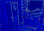
(e)

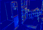
(f)

Fig. 12: Visual exhibition of shallow high-frequency features generated from LCF. (a) RGB image, (b) GT, (c) Bicubic, (d)-(f) high-frequency features.

Table 5: Different configurations for HR information. Scale $8\times$.

No.	HF Information	MSE	MAE
(I)	Canny Edge	12.0	1.13
(II)	Gaussian Edge	12.1	1.16
(III)	DCT	12.1	1.15
(IV)	Wavelet Transform	12.1	1.15
(V)	Gradient Map	11.8	1.12

Table 6: Effectiveness of HFEB. Scale $8\times$.

No.	Config.	Params (M)	Flops (G)	MSE	MAE
(I)	EdgeNet	5.78	95.6	12.0	1.12
(II)	SCPA	0.29	13.1	12.5	1.16
(III)	HFEB	0.27	11.6	11.8	1.12

4.4 Ablation Study

We now perform a series of ablation experiments to measure the impact of key components and parameters in DSR-EI. We collects the outcome of these studies, conducted on NYUv2 test set with $8\times$ factor. Without loss of fairness, NLSPN is never used here – to fully focus on the impact of single components. The configurations marked in gray in Tab. 4-Tab. 9 correspond to our final model without NLSPN.

(a) Implicit vs Explicit High-Frequency Features. To measure the impact of both implicit and explicit HR features, we compare the performance of the proposed network and its variants when extracting either only one of the two. The quantitative results are collected in Tab. 4. Without the help of gradient maps (I), the performance of the network significantly degrades. We believe this is caused by the difficulty in effectively extracting fine structures or salient edges required for LR depth maps from implicit HF features alone. Moreover, explicit features highlight regions in the image that need to be focused on, avoiding DSR-EI to learn to localize them and easing its task. Fig. 11 shows three among the high-frequency features $F_{edge}$ from a representative sample. We can notice how each of the three mainly emphasizes object boundaries, confirming the effectiveness of HFEB at extracting gradient information. At the same time, we can notice how the input RGB images expose very low texture, further confirming the effectiveness of HFEB at localizing high-frequency information.

Nonetheless, explicit HF features alone as guidance (II) are insufficient as well. We argue that the explicit information might neglect some RGB features, whereas implicit HF feature extraction can recover them. Furthermore, to verify the effectiveness of LCF, we replace it with ResBlock (He et al., 2016) (III) to extract shallow features from RGB images, highlighting a negative impact on implicit features extraction – i.e., it results less accurate than (II). Fig. 12 shows some of the features extracted by LCF. We can notice how, in addition to the primary high-frequency information, other information is encoded, such as semantics, which can further provide support for the explicit high-frequency information extracted in parallel by HFEB and improve the guidance for the final, depth super-resolution task.

(b) Ablation on Explicit High-Frequency Features. Based on the previous analysis, HFEB can significantly improve the network. To determine which high-frequency information is more suitable as guidance for GDSR, we experiment with five kinds of edge maps used as ground truth $E_{gt}$ to train HFEB: (1) the Canny edge map, (2) the Gaussian high-frequency map, (3) the high-frequency map generated by discrete cosine transform, (4) the high-frequency wavelet map and (5) the gradient map, as shown in Tab. 5. The Gaussian high-frequency map is obtained using a Gaussian filter, as detailed in Wang et al. (2020). Table 5 reports the outcome of the evaluation. From it, we can see that the Canny edge and the gradient map allow for better performance. Although DSR-EI with the gradient map attains the best results in terms of MSE and MAE, the different types of high-frequency maps do not significantly affect the final upsampling result.

(c) Impact of HFEB. To verify the effectiveness of HFEB, we replace it with EdgeNet (Liu et al., 2021) – based on the widely-used U-net structure – and SCPA (Zhao et al., 2020), which inspires our scaling strategy. As shown in Table 6, although the parameter size of EdgeNet is 5.6M, its performance is almost the same as our HFEB, while the parameter size of our network is only 0.7M, i.e. only $\frac{1}{8}$ of it. This fact highlights that our network based on a transformer is more efficient at feature extraction.

Besides, unlike previous works that employ fixed feature scaling rules, we adopt a dynamic scaling strategy to extract high-frequency features from depth maps. Table 6 also shows that our DSP with the dynamic scale strategy decreases the number of parameters while simultaneously enhancing the performance of GDSR. Compared to the original SCPA (Zhao et al., 2020), DSP can perform dynamic scaling according to the characteristics of the feature map to get a more effective receptive field.

Table 7: The impact of scales at which AFFM is applied.

No.	Scales	Params (M)	MSE	MAE
(I)	H1	1.5	12.3	1.14
(II)	H1, H2	3.0	11.8	1.12
(III)	H1, H2, H3	4.5	11.8	1.12

(d) Impact of AFFM. We now measure the effectiveness of AFFM. Tab. 8 shows results obtained by deploying AFFM at different scales, respectively the highest (I), the first two (II) and all of the three scales. We can notice how performing fusion at the highest scale alone results insufficient, whereas using multi-scale features for fusion yields improvements, despite saturating already when using two scales, with the lowest one not providing additional, meaningful details to be taken into account.

Furthermore, we ablate AFFM in its single components. Tab. 8 resumes the outcome of this evaluation. We first test the performance of DSR-EI without AFFM (I), highlighting a large drop in accuracy. By adding dynamic fusion, yet without using attention (II) vastly improves the results already, while replacing the weighted sum in the upper of Fig. 5 with concatenation and a ResBlock (He et al., 2016) (III) yields worse results compared to our full AFFM (IV).

Fig. 13 visualizes the attention maps produced by AFFM, highlighting how sharp and accurate they are in correspondence with depth discontinuities, tiny objects, and fine details. Thus, thanks to them AFFM can better focus on reconstructing depth boundaries and details more accurately.

Table 8: Ablation study of AFFM. Scale $8\times$.

No.	Config.	Params (M)	MSE	MAE
(I)	w/o AFFM	-	12.7	1.16
(II)	w/o att	1.3	12.2	1.13
(III)	Concat.	4.5	12.2	1.13
(IV)	AFFM	3.0	11.8	1.12

(a)

(b)

(c)

(d)

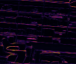
(e)

(f)

(g)

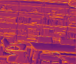
(h)

Fig. 13: Visual exhibition of attention maps generated from AFFM. (a) RGB image, (b) GT, (c) Bicubic, (d)-(h) attention maps.

Table 9: Comparisons with different stage numbers. Scale $8\times$.

No.	Stages	Params (M)	MSE	MAE
(I)	$1$	14.2	13.3	1.19
(II)	$2$	25.0	11.8	1.12
(III)	$3$	37.5	11.6	1.10

(e) Impact of Stages Number. To conclude, we evaluate the impact of the multi-stage design. As shown in Tab. 9, a single-stage architecture (I) is vastly outperformed by deploying two stages (II), yet at the expense of doubling the number of parameters. Furthermore, while the three-stage architecture (III) still yields some improvement, the benefit is minor in comparison to the significant increase in parameters. Hence, we choose two stages as the default configuration to balance accuracy and efficiency.

Table 10: Results on NYUv2 and DIML dataset – different input sizes. We report MSE (cm²) / MAE (cm), the lower the better.

Method	Size	DIML			Size	NYUv2
		4$\times$	8$\times$	16$\times$		4$\times$	8$\times$	16$\times$
DSR-EI+	256$\times$256	0.65 / 0.12	2.09 / 0.22	6.31 / 0.50	256$\times$256	2.75 / 0.47	11.8 / 1.09	47.1 / 2.40
	1344$\times$756	0.58 / 0.12	1.91 / 0.20	5.15 / 0.45	640$\times$480	1.93 / 0.39	8.14 / 0.89	33.0 / 2.02

Table 11: Computational requirements at inference. Experiments on Nvidia RTX 3090 GPU, with $256\times 256$ input and $8\times$ factor.

	PMBANet	FDSR	JIIF	DCTNet	LGR	Ours
Runtime (ms)	26.9	1.03	89.8	9.03	26.4	51.5
Memory Peak (GB)	3.07	2.05	2.36	0.26	0.19	18.6

(f) Results on full-size images. In Tab. 1 and 2, we reported the results achieved by our model when processing $256\times 256$ patches, to allow for a fair comparison with LGR (de Lutio et al., 2022) and DADA (Metzger et al., 2022). However, this irremediably reduces the global context processed by DSR-EI, hindering its capacity to exploit it enabled by the transformer blocks similar to what was observed in the generalization experiment on Middlebury (Tab. 4). In this section, we demonstrate how processing larger images allows DSR-EI to further improve its performance. Tab. 10 compares the results achieved when switching from $256\times 256$ patches to the full resolution images of DIML and NYUv2 – i.e., $1344\times 756$ and $640\times 480$, respectively. We can notice consistent improvements, particularly when dealing with larger upsampling factors.

4.5 Limitations

We conclude by listing a few limitations of DSR-EI. As previously pointed out, global context is crucial for it to achieve the best performance. When this is unavailable, some accuracy is lost when generalizing across datasets. Moreover, the significant improvements over existing methods are paid for in terms of time/memory requirements. Tab. 11 highlights the higher runtime and, more evidently, peak memory usage. Future work will aim at reducing the overhead, while minimizing the drop in accuracy.

5 Conclusion

This paper proposed DSR-EI, a depth super-resolution network, which includes a high-frequency extraction branch (HFEB) and a guided depth restoration branch (GDRB). Specifically, implemented as an efficient transformer, HFEB extracts explicit HF features. Then, GDRB deploys a two-stage encoder-decoder network to recover HR depth maps progressively, by adaptively fusing discriminative features while supplementing additional, implicit HF information. Exhaustive experiments demonstrate that DSR-EI sets a new state-of-the-art for guided depth super-resolution.

References

- Bamji et al. (2022) Bamji, C., Godbaz, J., Oh, M., Mehta, S., Payne, A., Ortiz, S., Nagaraja, S., Perry, T., Thompson, B., 2022. A review of indirect time-of-flight technologies. IEEE Transactions on Electron Devices .
- Cai et al. (2010) Cai, Q., Gallup, D., Zhang, C., Zhang, Z., 2010. 3d deformable face tracking with a commodity depth camera, in: European conference on computer vision, Springer. pp. 229–242.
- Carion et al. (2020) Carion, N., Massa, F., Synnaeve, G., Usunier, N., Kirillov, A., Zagoruyko, S., 2020. End-to-end object detection with transformers, in: European conference on computer vision, Springer. pp. 213–229.
- Chang et al. (2007) Chang, C.C., Lin, C.C., Tseng, C.S., Tai, W.L., 2007. Reversible hiding in dct-based compressed images. Information Sciences 177, 2768–2786.
- Chen et al. (2020a) Chen, X., Lin, K.Y., Qian, C., Zeng, G., Li, H., 2020a. 3d sketch-aware semantic scene completion via semi-supervised structure prior, in: Proceedings of the IEEE/CVF Conference on Computer Vision and Pattern Recognition, pp. 4193–4202.
- Chen et al. (2020b) Chen, X., Xing, Y., Zeng, G., 2020b. Real-time semantic scene completion via feature aggregation and conditioned prediction, in: 2020 IEEE International Conference on Image Processing (ICIP), IEEE. pp. 2830–2834.
- Chen et al. (2020c) Chen, Y., Dai, X., Liu, M., Chen, D., Yuan, L., Liu, Z., 2020c. Dynamic convolution: Attention over convolution kernels, in: Proceedings of the IEEE/CVF Conference on Computer Vision and Pattern Recognition, pp. 11030–11039.
- Chen et al. (2018) Chen, Y., Wang, Z., Peng, Y., Zhang, Z., Yu, G., Sun, J., 2018. Cascaded pyramid network for multi-person pose estimation, in: Proceedings of the IEEE conference on computer vision and pattern recognition, pp. 7103–7112.
- Chen et al. (2021) Chen, Z., Cong, R., Xu, Q., Huang, Q., 2021. Dpanet: Depth potentiality-aware gated attention network for rgb-d salient object detection. IEEE Transactions on Image Processing 30, 7012–7024. doi:10.1109/TIP.2020.3028289.
- Cho et al. (2021) Cho, J., Min, D., Kim, Y., Sohn, K., 2021. Deep monocular depth estimation leveraging a large-scale outdoor stereo dataset. Expert Systems with Applications 178, 114877.
- Deng and Dragotti (2020) Deng, X., Dragotti, P.L., 2020. Deep convolutional neural network for multi-modal image restoration and fusion. IEEE transactions on pattern analysis and machine intelligence 43, 3333–3348.
- Diebel and Thrun (2005) Diebel, J., Thrun, S., 2005. An application of markov random fields to range sensing. Advances in neural information processing systems 18.
- Dosovitskiy et al. (2021) Dosovitskiy, A., Beyer, L., Kolesnikov, A., Weissenborn, D., Zhai, X., Unterthiner, T., Dehghani, M., Minderer, M., Heigold, G., Gelly, S.a., 2021. An image is worth 16x16 words: Transformers for image recognition at scale, in: International Conference on Learning Representations.
- Farha and Gall (2019) Farha, Y.A., Gall, J., 2019. Ms-tcn: Multi-stage temporal convolutional network for action segmentation, in: Proceedings of the IEEE/CVF Conference on Computer Vision and Pattern Recognition, pp. 3575–3584.
- Ferstl et al. (2013) Ferstl, D., Reinbacher, C., Ranftl, R., Rüther, M., Bischof, H., 2013. Image guided depth upsampling using anisotropic total generalized variation, in: Proceedings of the IEEE international conference on computer vision, pp. 993–1000.
- Gao et al. (2019) Gao, H., Tao, X., Shen, X., Jia, J., 2019. Dynamic scene deblurring with parameter selective sharing and nested skip connections, in: Proceedings of the IEEE/CVF conference on computer vision and pattern recognition, pp. 3848–3856.
- Ge et al. (2019) Ge, L., Liang, H., Yuan, J., Thalmann, D., 2019. Real-time 3d hand pose estimation with 3d convolutional neural networks. IEEE Transactions on Pattern Analysis and Machine Intelligence 41, 956–970. doi:10.1109/TPAMI.2018.2827052.
- Ham et al. (2017) Ham, B., Cho, M., Ponce, J., 2017. Robust guided image filtering using nonconvex potentials. IEEE transactions on pattern analysis and machine intelligence 40, 192–207.
- Han et al. (2022) Han, K., Wang, Y., Chen, H., Chen, X., Guo, J., Liu, Z., Tang, Y., Xiao, A., Xu, C., Xu, Y., et al., 2022. A survey on vision transformer. IEEE transactions on pattern analysis and machine intelligence .
- He et al. (2010) He, K., Sun, J., Tang, X., 2010. Guided image filtering, in: European conference on computer vision, Springer. pp. 1–14.
- He et al. (2016) He, K., Zhang, X., Ren, S., Sun, J., 2016. Deep residual learning for image recognition, in: Proceedings of the IEEE conference on computer vision and pattern recognition, pp. 770–778.
- He et al. (2021) He, L., Zhu, H., Li, F., Bai, H., Cong, R., Zhang, C., Lin, C., Liu, M., Zhao, Y., 2021. Towards fast and accurate real-world depth super-resolution: Benchmark dataset and baseline, in: Proceedings of the IEEE/CVF Conference on Computer Vision and Pattern Recognition, pp. 9229–9238.
- Hirschmuller and Scharstein (2007) Hirschmuller, H., Scharstein, D., 2007. Evaluation of cost functions for stereo matching, in: 2007 IEEE Conference on Computer Vision and Pattern Recognition, IEEE. pp. 1–8.
- Huang et al. (2022) Huang, T., Huang, L., You, S., Wang, F., Qian, C., Xu, C., 2022. Lightvit: Towards light-weight convolution-free vision transformers. arXiv preprint arXiv:2207.05557 .
- Hui et al. (2016) Hui, T.W., Loy, C.C., Tang, X., 2016. Depth map super-resolution by deep multi-scale guidance, in: European conference on computer vision, Springer. pp. 353–369.
- Kiechle et al. (2013) Kiechle, M., Hawe, S., Kleinsteuber, M., 2013. A joint intensity and depth co-sparse analysis model for depth map super-resolution, in: Proceedings of the IEEE international conference on computer vision, pp. 1545–1552.
- Kim et al. (2021) Kim, B., Ponce, J., Ham, B., 2021. Deformable kernel networks for joint image filtering. International Journal of Computer Vision 129, 579–600.
- Kim et al. (2022) Kim, K., Lee, S., Cho, S., 2022. Mssnet: Multi-scale-stage network for single image deblurring. arXiv preprint arXiv:2202.09652 .
- Kim et al. (2017) Kim, S., Min, D., Ham, B., Kim, S., Sohn, K., 2017. Deep stereo confidence prediction for depth estimation, in: 2017 ieee international conference on image processing (icip), IEEE. pp. 992–996.
- Kim et al. (2016) Kim, Y., Ham, B., Oh, C., Sohn, K., 2016. Structure selective depth superresolution for rgb-d cameras. IEEE Transactions on Image Processing 25, 5227–5238.
- Kim et al. (2018) Kim, Y., Jung, H., Min, D., Sohn, K., 2018. Deep monocular depth estimation via integration of global and local predictions. IEEE transactions on Image Processing 27, 4131–4144.
- Kopf et al. (2007) Kopf, J., Cohen, M.F., Lischinski, D., Uyttendaele, M., 2007. Joint bilateral upsampling. ACM Transactions on Graphics (ToG) 26, 96–es.
- Kwon et al. (2015) Kwon, H., Tai, Y.W., Lin, S., 2015. Data-driven depth map refinement via multi-scale sparse representation, in: Proceedings of the IEEE conference on computer vision and pattern recognition, pp. 159–167.
- Lee et al. (2022) Lee, Y., Kim, J., Willette, J., Hwang, S.J., 2022. Mpvit: Multi-path vision transformer for dense prediction, in: Proceedings of the IEEE/CVF Conference on Computer Vision and Pattern Recognition, pp. 7287–7296.
- Li et al. (2016a) Li, Y., Huang, J.B., Ahuja, N., Yang, M.H., 2016a. Deep joint image filtering, in: European conference on computer vision, Springer. pp. 154–169.
- Li et al. (2019) Li, Y., Huang, J.B., Ahuja, N., Yang, M.H., 2019. Joint image filtering with deep convolutional networks. IEEE transactions on pattern analysis and machine intelligence 41, 1909–1923.
- Li et al. (2016b) Li, Y., Min, D., Do, M.N., Lu, J., 2016b. Fast guided global interpolation for depth and motion, in: European Conference on Computer Vision, Springer. pp. 717–733.
- Lin et al. (2010) Lin, S.D., Shie, S.C., Guo, J.Y., 2010. Improving the robustness of dct-based image watermarking against jpeg compression. Computer Standards & Interfaces 32, 54–60.
- Liu et al. (2022) Liu, P., Zhang, Z., Meng, Z., Gao, N., Wang, C., 2022. Pdr-net: Progressive depth reconstruction network for color guided depth map super-resolution. Neurocomputing 479, 75–88.
- Liu et al. (2021) Liu, Y., Fang, F., Wang, T., Li, J., Sheng, Y., Zhang, G., 2021. Multi-scale grid network for image deblurring with high-frequency guidance. IEEE Transactions on Multimedia .
- de Lutio et al. (2022) de Lutio, R., Becker, A., D’Aronco, S., Russo, S., Wegner, J.D., Schindler, K., 2022. Learning graph regularisation for guided super-resolution, in: Proceedings of the IEEE/CVF Conference on Computer Vision and Pattern Recognition, pp. 1979–1988.
- Lutio et al. (2019) Lutio, R.d., D’aronco, S., Wegner, J.D., Schindler, K., 2019. Guided super-resolution as pixel-to-pixel transformation, in: Proceedings of the IEEE/CVF International Conference on Computer Vision, pp. 8829–8837.
- Mac Aodha et al. (2012) Mac Aodha, O., Campbell, N.D., Nair, A., Brostow, G.J., 2012. Patch based synthesis for single depth image super-resolution, in: European conference on computer vision, Springer. pp. 71–84.
- Metzger et al. (2022) Metzger, N., Daudt, R.C., Schindler, K., 2022. Guided depth super-resolution by deep anisotropic diffusion. arXiv preprint arXiv:2211.11592 .
- Pan et al. (2019) Pan, J., Dong, J., Ren, J.S., Lin, L., Tang, J., Yang, M.H., 2019. Spatially variant linear representation models for joint filtering, in: Proceedings of the IEEE/CVF Conference on Computer Vision and Pattern Recognition, pp. 1702–1711.
- Park et al. (2020) Park, J., Joo, K., Hu, Z., Liu, C.K., So Kweon, I., 2020. Non-local spatial propagation network for depth completion, in: European Conference on Computer Vision, Springer. pp. 120–136.
- Park et al. (2011) Park, J., Kim, H., Tai, Y.W., Brown, M.S., Kweon, I., 2011. High quality depth map upsampling for 3d-tof cameras, in: 2011 International Conference on Computer Vision, IEEE. pp. 1623–1630.
- Paszke et al. (2019) Paszke, A., Gross, S., Massa, F., Lerer, A., Bradbury, J., Chanan, G., Killeen, T., Lin, Z., Gimelshein, N., Antiga, L., et al., 2019. Pytorch: An imperative style, high-performance deep learning library. Advances in neural information processing systems 32.
- Pu et al. (2022) Pu, M., Huang, Y., Liu, Y., Guan, Q., Ling, H., 2022. Edter: Edge detection with transformer, in: Proceedings of the IEEE/CVF Conference on Computer Vision and Pattern Recognition, pp. 1402–1412.
- Qin et al. (2021) Qin, Z., Zhang, P., Wu, F., Li, X., 2021. Fcanet: Frequency channel attention networks, in: Proceedings of the IEEE/CVF international conference on computer vision, pp. 783–792.
- Riemens et al. (2009) Riemens, A., Gangwal, O., Barenbrug, B., Berretty, R.P., 2009. Multistep joint bilateral depth upsampling, in: Visual communications and image processing 2009, SPIE. pp. 192–203.
- Ronneberger et al. (2015) Ronneberger, O., Fischer, P., Brox, T., 2015. U-net: Convolutional networks for biomedical image segmentation, in: International Conference on Medical image computing and computer-assisted intervention, Springer. pp. 234–241.
- Sarlin et al. (2019) Sarlin, P.E., Cadena, C., Siegwart, R., Dymczyk, M., 2019. From coarse to fine: Robust hierarchical localization at large scale, in: Proceedings of the IEEE/CVF Conference on Computer Vision and Pattern Recognition, pp. 12716–12725.
- Scharstein et al. (2014) Scharstein, D., Hirschmüller, H., Kitajima, Y., Krathwohl, G., Nešić, N., Wang, X., Westling, P., 2014. High-resolution stereo datasets with subpixel-accurate ground truth, in: German conference on pattern recognition, Springer. pp. 31–42.
- Scharstein and Pal (2007) Scharstein, D., Pal, C., 2007. Learning conditional random fields for stereo, in: 2007 IEEE Conference on Computer Vision and Pattern Recognition, IEEE. pp. 1–8.
- Scharstein and Szeliski (2003) Scharstein, D., Szeliski, R., 2003. High-accuracy stereo depth maps using structured light, in: 2003 IEEE Computer Society Conference on Computer Vision and Pattern Recognition, 2003. Proceedings., IEEE. pp. I–I.
- Silberman et al. (2012) Silberman, N., Hoiem, D., Kohli, P., Fergus, R., 2012. Indoor segmentation and support inference from rgbd images, in: European conference on computer vision, Springer. pp. 746–760.
- Su et al. (2019) Su, H., Jampani, V., Sun, D., Gallo, O., Learned-Miller, E., Kautz, J., 2019. Pixel-adaptive convolutional neural networks, in: Proceedings of the IEEE/CVF Conference on Computer Vision and Pattern Recognition, pp. 11166–11175.
- Tang et al. (2021a) Tang, J., Chen, X., Zeng, G., 2021a. Joint implicit image function for guided depth super-resolution, in: Proceedings of the 29th ACM International Conference on Multimedia, pp. 4390–4399.
- Tang et al. (2021b) Tang, Q., Cong, R., Sheng, R., He, L., Zhang, D., Zhao, Y., Kwong, S., 2021b. Bridgenet: A joint learning network of depth map super-resolution and monocular depth estimation, in: Proceedings of the 29th ACM International Conference on Multimedia, pp. 2148–2157.
- Touvron et al. (2021) Touvron, H., Cord, M., Douze, M., Massa, F., Sablayrolles, A., Jégou, H., 2021. Training data-efficient image transformers & distillation through attention, in: International Conference on Machine Learning, PMLR. pp. 10347–10357.
- Vaswani et al. (2017) Vaswani, A., Shazeer, N., Parmar, N., Uszkoreit, J., Jones, L., Gomez, A.N., Kaiser, Ł., Polosukhin, I., 2017. Attention is all you need. Advances in neural information processing systems 30.
- Wang et al. (2019) Wang, H., Kembhavi, A., Farhadi, A., Yuille, A.L., Rastegari, M., 2019. Elastic: Improving cnns with dynamic scaling policies, in: Proceedings of the IEEE/CVF Conference on Computer Vision and Pattern Recognition, pp. 2258–2267.
- Wang et al. (2021) Wang, W., Xie, E., Li, X., Fan, D.P., Song, K., Liang, D., Lu, T., Luo, P., Shao, L., 2021. Pyramid vision transformer: A versatile backbone for dense prediction without convolutions, in: Proceedings of the IEEE/CVF International Conference on Computer Vision, pp. 568–578.
- Wang et al. (2014) Wang, Y., Ortega, A., Tian, D., Vetro, A., 2014. A graph-based joint bilateral approach for depth enhancement, in: 2014 IEEE International Conference on Acoustics, Speech and Signal Processing (ICASSP), IEEE. pp. 885–889.
- Wang et al. (2020) Wang, Z., Ye, X., Sun, B., Yang, J., Xu, R., Li, H., 2020. Depth upsampling based on deep edge-aware learning. Pattern Recognition 103, 107274.
- Yang et al. (2007) Yang, Q., Yang, R., Davis, J., Nistér, D., 2007. Spatial-depth super resolution for range images, in: 2007 IEEE Conference on Computer Vision and Pattern Recognition, IEEE. pp. 1–8.
- Ye et al. (2020) Ye, X., Sun, B., Wang, Z., Yang, J., Xu, R., Li, H., Li, B., 2020. Pmbanet: Progressive multi-branch aggregation network for scene depth super-resolution. IEEE Transactions on Image Processing 29, 7427–7442.
- Yuan et al. (2023) Yuan, J., Jiang, H., Li, X., Qian, J., Li, J., Yang, J., 2023. Recurrent structure attention guidance for depth super-resolution. arXiv preprint arXiv:2301.13419 .
- Zamir et al. (2022) Zamir, S.W., Arora, A., Khan, S., Hayat, M., Khan, F.S., Yang, M.H., 2022. Restormer: Efficient transformer for high-resolution image restoration, in: Proceedings of the IEEE/CVF Conference on Computer Vision and Pattern Recognition, pp. 5728–5739.
- Zamir et al. (2021) Zamir, S.W., Arora, A., Khan, S., Hayat, M., Khan, F.S., Yang, M.H., Shao, L., 2021. Multi-stage progressive image restoration, in: Proceedings of the IEEE/CVF conference on computer vision and pattern recognition, pp. 14821–14831.
- Zhang et al. (2018) Zhang, Y., Li, K., Li, K., Wang, L., Zhong, B., Fu, Y., 2018. Image super-resolution using very deep residual channel attention networks, in: Proceedings of the European conference on computer vision (ECCV), pp. 286–301.
- Zhao et al. (2020) Zhao, H., Kong, X., He, J., Qiao, Y., Dong, C., 2020. Efficient image super-resolution using pixel attention, in: European Conference on Computer Vision Workshops, Springer. pp. 56–72.
- Zhao et al. (2022) Zhao, Z., Zhang, J., Xu, S., Lin, Z., Pfister, H., 2022. Discrete cosine transform network for guided depth map super-resolution, in: Proceedings of the IEEE/CVF Conference on Computer Vision and Pattern Recognition, pp. 5697–5707.
- Zou et al. (2022) Zou, X., Xiao, F., Yu, Z., Li, Y., Lee, Y.J., 2022. Delving deeper into anti-aliasing in convnets. International Journal of Computer Vision , 1–15.
- Zuo et al. (2020) Zuo, Y., Fang, Y., An, P., Shang, X., Yang, J., 2020. Frequency-dependent depth map enhancement via iterative depth-guided affine transformation and intensity-guided refinement. IEEE Transactions on Multimedia 23, 772–783.