Exploring Resiliency to Natural Image Corruptions in Deep Learning using Design Diversity

Abstract

In this paper, we investigate the relationship between diversity metrics, accuracy, and resiliency to natural image corruptions of Deep Learning (DL) image classifier ensembles. We investigate the potential of an attribution-based diversity metric to improve the known accuracy-diversity trade-off of the typical prediction-based diversity. Our motivation is based on analytical studies of design diversity that have shown that a reduction of common failure modes is possible if diversity of design choices is achieved.

Using ResNet50 as a comparison baseline, we evaluate the resiliency of multiple individual DL model architectures against dataset distribution shifts corresponding to natural image corruptions. We compare ensembles created with diverse model architectures trained either independently or through a Neural Architecture Search technique and evaluate the correlation of prediction-based and attribution-based diversity to the final ensemble accuracy. We evaluate a set of diversity enforcement heuristics based on negative correlation learning to assess the final ensemble resilience to natural image corruptions and inspect the resulting prediction, activation, and attribution diversity.

Our key observations are: 1) model architecture is more important for resiliency than model size or model accuracy, 2) attribution-based diversity is less negatively correlated to the ensemble accuracy than prediction-based diversity, 3) a balanced loss function of individual and ensemble accuracy creates more resilient ensembles for image natural corruptions, 4) architecture diversity produces more diversity in all explored diversity metrics: predictions, attributions, and activations.

1 Introduction

In the context of Deep Learning (DL), it has been empirically discovered that the use of ensembles can improve the model’s accuracy in tasks such as regression and classification. It has been speculated [13] that the main reason behind these improvements is the implicit diversity in the solutions found that when aggregated as an ensemble obtain better predictions. In this work, we evaluate the resiliency of diverse deep learning classifiers and the role that the different kinds of diversity play in improving them.

1.1 The case for design diversity

Design diversity [23] is a technique to increase the resilience of safety critical systems. It is established as a best practice in standards such as in vehicle functional safety  [18] to prevent dependent failures, safety of the intended functionality  [19] to address system limitations of machine-learning-based components, and avionic software [12].

A common pitfall is to misunderstand independent development as design diversity. In [47] the designers of a safety-critical system preferred to let multiple teams collaborate, although the purpose of having multiple teams is to produce multiple designs of a single specification. This was justified with the claim that specification problems can be better mitigated with such collaboration but at the cost of the sought independence.

The key problem is, that independent development can (and will) produce designs with common failures mainly due to the fact that independent designs do not enforce diverse design choices. In fact, it has been statistically proven that independently developed software results in dependent failure behavior on randomly selected inputs [11].

In [22], it has been shown that what is needed to reduce dependent failure behavior is diversity in design choices. If the choices are made satisfying certain properties, it can be expected (in the average case) to obtain negatively correlated failure behavior, i.e., better than independent.

In DL, however, design choices are not made by the human designers explicitly but are a result of the architecture, data, and optimization approach. Furthermore, existing diversity metrics are not directly related to the DL model’s design choices and are known to have a diversity-accuracy trade-off [21]. We investigate if a diversity metric closer to the model design choices can improve the model resilience compared to existing metrics.

1.2 Main research questions

We aim to answer the following research questions:
RQ1: Is model accuracy, size, or architecture the main explanatory factor of resilience against natural image corruptions?
RQ2: Can a diversity metric closer to design choices improve the known accuracy-diversity trade-off?
RQ3: Which diversity enforcement heuristic produces the most resilient models?
RQ4: How diverse are the predictions, activations, and input feature attributions of models created with a diversity enforcement learning approach?

The rest of the paper is structured as follows: Section 2 provides a brief overview of the current state-of-the-art in diversity enforcement and measurement. Next, the methodology is stated in Section 3. Our experiments are then presented in Section 4, followed by a discussion of the outcomes and conclusions in Section 5.

2 Related work

2.1 Ensemble creation techniques

The most relevant techniques for ensemble creation are: a) Ensembles of independently trained models where diversity originates from the training process randomness, e.g., seed. Each ensemble member loss is a function notated as:

$$l(h^{i},y)$$ (1)

where $y$ is the ground-truth label, and $h^{i}$ is the output of the $i$th single ensemble member. [6] presents an analysis of the resilience of independently trained ensembles. b) Bagging [1], reduces the variance of multiple models by averaging the outcomes of models created with different training data subsets. c) Boosting [37] sequentially trains models to reduce bias by sampling incorrectly classified inputs more often in the next model. d) Negative Correlation Learning (NCL) [24] trains models in parallel with a shared penalty term in their loss function to enforce prediction diversity. Generalized NCL (GNCL) [3] proposes two extensions for NCL: i) a generalized loss function for each member:

$$\sum_{i=1}^{M}{l(h^{i},y)-\frac{\lambda}{2M}\sum_{i=1}^{M}{{d_{i}}^{T}\mathfrak{D}d_{i}}}$$ (2)

where $M$ is the total number of members in the ensemble, $d$ is the difference $h^{i}-f$ with $f$ as the ensemble prediction, $\mathfrak{D}$ is the 2nd derivative of the loss function, and $\lambda$ is a weighting hyper-parameter. ii) An implicit enforcement of diversity by balancing the ensemble and the individual loss:

$$\frac{1}{M}\sum_{i=1}^{M}{\big{(}\lambda{l(f,y)}+\frac{1-\lambda}{M}\sum_{i=1}^{M}{l(h^{i},y)}\big{)}}$$ (3)

2.2 Diversity metrics in DL

There are many proposed metrics for diversity. [2] presents a survey and taxonomy for diversity metrics and [14] presents a survey of diversity for ML. In this work, we focus on behavior diversity metrics of a DL model. Input data diversity such as different modalities or implementation aspects such as the number of layers is not considered.

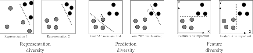
Figure 1: Model behavior diversity. a) Invariant decision boundary & diverse sample representation. b) Diverse decision boundary and measured by prediction errors. c) Diverse decision boundary and measured by feature relevance.

Prediction (output, failures) diversity Multiple prediction-based diversity metrics have been proposed. [21] presents a comprehensive evaluation of this class of metrics. Pair-wise measures based on the correct and incorrect statistics of two models include the Q-statistics, correlation coefficient $\rho$, and the disagreement measure:

$$D_{p,q}=\frac{N^{01}+N^{10}}{N^{11}+N^{10}+N^{01}+N^{00}}$$ (4)

where the indexes $a,b$ of the binary vectors $N^{ab}$ indicate the correctness of the classifiers, i.e., $(h^{i=p}=y)\Rightarrow(a=1)\wedge(h^{i=p}\neq{y})\rightarrow(a=0)$. Non-pairwise measures that evaluate non-binary diversity include entropy, coincident failure diversity, cosine similarity, Kullback–Leibler divergence [10, 31], and the the Shannon equitability index [32, 6]:

$$E=-\sum_{i=1}^{S}{p_{i}\ln{p_{i}}}\big{/}\ln{S}$$ (5)

where $S$ is the total number of prediction species/classes and $p_{i}$ is the proportion of observed species $i$.

Representation (activation) diversity The intermediate representations (IR) can also be used to measure diversity. [13] compares the diversity in representation space from independently created ensembles and ensembles from variational approaches. Measuring IR diversity is challenging due to space size and semantic ambiguity, i.e., the same semantic concept can be represented in many different ways. A naive use of any diversity metric such as cosine similarity could give semantically irrelevant diversity scores. In [20], the Centered Kernel Alignment (CKA) metric is proposed to obtain a statistical measure across a dataset on the similarity of any two layers of a DL model:

$$\text{CKA}(K,L)=\frac{\text{HSIC}(K,L)}{\sqrt{\text{HSIC}(K,K)\text{HSIC}(L,L)}}$$ (6)

where $K$ and $L$ are similarity matrices of the two feature maps being compared and HSIC is the Hilbert-Schmidt Independence Criterion which measures statistical independence. The feature maps may be layer activations or attention maps such as Saliency, Integrated Gradients, and Grad-CAM [40, 39, 41].

[34] proposed the use of the pull-away loss term from generative adversarial networks to induce diversity of such activations. Self-attention [45] (not related to attention maps) is one of the key techniques in the transformer architecture. In [33] the embeddings used to feed attention heads are masked in such a way as to enforce diversity of activations. In zero-shot learning, the attribute concept is used to enable training models that can, later on, predict unseen labels. These attributes can be considered for IR diversity, as well  [48]. Closely related to NCL, the self-supervised approach of contrastive learning [38, 7] trains two models to produce latent features that are diverse for false positive cases and similar in true positives through a loss function such as the triplet loss that enforces the models to learn the similarity metric.

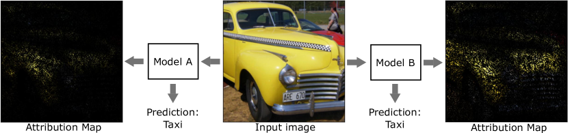
Figure 2: Attribution map diversity: Two models may predict the same outcome but based on different evidence.

Input feature attribution diversity The importance of input features can be used to measure behavior diversity that to the best of our knowledge has not been explored. Figure 1 shows the relationship of an attribution-based metric w.r.t. prediction and representation diversity. Note, that attribution is not the same as attention or attributes in the context of zero-shot learning. Attention maps, such as those obtained from the activation of intermediate layers of CNNs, reflect the excitation of a network given an input. This activation however is not necessarily correlated with the final prediction, e.g., it could be an inhibitory factor. Attribution, on the other hand, indicates the importance of a feature to the final decision. See Figure 2 where Saliency is used to display the original pixels masked by the attribution scores from each model. A change to a pixel with high attribution (brighter) will have a stronger influence on the model prediction than a change to a pixel with low attribution.

2.3 Other diversity-based resilience approaches

Augmenting the training data by applying affine transformations such as rotations and scaling, geometric distortions such as blurring, and texture transfer help DL models to generalize better with a limited training data [27]. Adversarial training increases the robustness to intended attacks with adversarial samples to limit the model vulnerability to input perturbations [15]. Such training data approaches are effective and complementary to the design diversity approaches of this study that address the model diversity.

Modality and point of view diversity [35] is an approach to address the failure modes of sensors such as cameras, radar, and lidar. The design diversity of DL models explored in this study is orthogonal to this approach, as model diversity can be applied to every single modality.

3 Methodology

We propose three sets of experiments:

1. Evaluate resiliency of diverse architectures and training approaches.

2. Measure diversity of prediction and diversity of attribution from independently created models of diverse architectures and evaluate robustness correlation.

3. Enforce diversity with NCL, evaluate the resulting robustness, and inspect three kinds of diversity: prediction, representation, and attribution.

In addition to addressing the main research questions, we put the following hypothesis to test: that attribution-based diversity (Equation 7) can be positively correlated with ensemble resiliency if a better accuracy trade-off is achieved compared to prediction-based diversity.

$$A={\sum_{c=1}^{C}{\sum_{p=1}^{P}{Var(a_{c,p})}}}$$ (7)

where $a$ is the input attribution score of a model at color channel $c$ and pixel coordinate $p$. The computation of the input attribution scores $a$ is performed with an attribution method, such as Saliency.

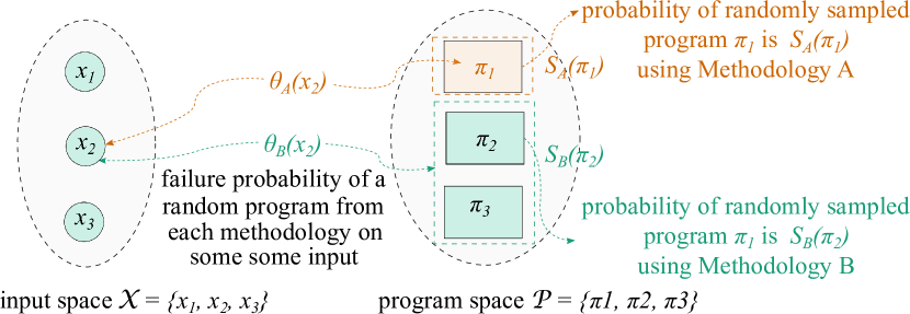
Figure 3: Relation between diverse design methodologies and the difficulty function in the LM Model [22]

This hypothesis is inspired by the theoretical result of the Littlewood and Miller (LM) model [22] that diverse design choices can produce less common failures. Diverse attribution maps of correct classifications imply that the models make predictions based on independent factors, which is not the case in prediction diversity.

3.1 Probability model for design diversity (LM model)

The Littlewood and Miller (LM) model [22] defines a probabilistic framework to analyze the impact of methodological diversity in the expected failure behavior. The model defines: 1) an input space $\mathcal{X}=\{x_{1},x_{2},...\}$, representing all possible inputs $x$ to a program and 2) a program space $\mathcal{P}=\{(\pi_{1},\pi_{2})\}$, for all possible programs $\pi$ that could implement a program specification. A given design methodology will determine the probability to come up with a program $\pi$ and is denoted as $S_{A}(\pi)$. Another design methodology $S_{B}(\pi)$ will assign a different probability to the same program. The model uses the concept of a difficulty function $\theta_{M}(x)$ that measures the probability that a randomly chosen program $\pi$ from a given methodology distribution $S_{M}(\pi)$ will fail on a particular input $x\in\mathcal{X}$. The key insight consists in noticing that $\theta_{A}(x)$ can be different for a different methodology $\theta_{B}(x)$, i.e., for some methodology, a certain input may be difficult, but for another, it may be easy. See Figure 3 for a visual representation of these spaces. An analysis of this model concludes that if the design methodologies produce different difficulty functions $\theta$, then the expected failure behavior on a random input will be negatively correlated due to the fact that the covariance of the $\theta$’s can be negative.

With this model, it is finally shown that a design methodology with diverse design choices that satisfy the following three properties will result in less common failures: 1) logically unrelated (one decision is independent of the other), 2) common failures of a decision are due to different factors, and 3) indifference to the selection of each methodology (no methodology is superior).

3.2 Loss function to enforce attribution diversity

We perform a first attempt to enforce attribution diversity with the following loss:

$$\frac{1}{M}\sum_{i=1}^{M}{l(h^{i},y)}-\lambda{A}$$ (8)

This loss computes attribution scores variance in an ensemble and uses it as a penalty term weighted by $\lambda$.

3.3 Failures addressed

In this study, we evaluate resilience to covariate dataset distribution shifts, i.e., when the distribution of input features of the test dataset does not match the distribution of the training dataset. We use four natural image perturbations from the ImageNet-$\overline{\mbox{C}}$ dataset [28] that are sensible to occur in vision application domains, such as obstructions or liquid contaminants. Our scope is not to evaluate robustness against adversarial attacks, label shift variations, or resiliency to noise variations such as Gaussian, brown, etc.

4 Experimental results

4.1 ML resiliency to data corruptions

To understand the relationship between accuracy, size, and resiliency to natural corruptions of DL models we evaluate a set of architectures (convolutional NNs, transformers, and subnetworks from neural architecture search (NAS)) and training approaches (supervised, self-supervised, and knowledge distillation) on both the ImageNet validation dataset and on the corrupted version ImageNet-$\overline{\mbox{C}}$ ”Lines” (strength of 1.6). See Table 1.

Table 1: Resiliency of architectures to natural image corruption (ImageNet-$\overline{\mbox{C}}$ Lines(1.6 strength))

Training	Arch.	DL model	#	ImageNet		ImageNet-$\overline{\mbox{C}}$
approach	class		Params			Lines1.6
				top1	top5	top1	top5
Self-sup.	CNN	DINO ResNet50 [5]	25.6M	75.30	92.61	21.80	40.66
Superv.	CNN	ResNet50 [16]	25.6M	75.85	92.88	34.95	55.88
Superv.	CNN	ResNext50_32_4d [46]	25.0M	77.49	93.57	39.46	60.61
Superv.	CNN	ResNet152 [16]	60.2M	78.25	93.96	40.17	62.09
Superv.	NAS	EfficientNet_b7 [43]	66.3M	74.82	92.13	51.11	73.81
Superv.	CNN	ResNext101_64x4d [46]	83.4M	82.90	96.22	51.89	72.46
Superv.	ViT	Swin tiny [26]	28.3M	81.34	95.612	55.29	78.45
Self-sup.	ViT	DINO ViT_b_8 [5]	87.3M	80.06	95.02	55.75	78.37
Superv.	ViT	Swin base [26]	87.8M	83.30	96.46	58.71	81.05
Superv.	ViT	ViT base p16 [9]	86.6M	80.88	95.28	61.28	82.26
K. distill.	ViT	DeiT-base [44]	87.3M	83.34	96.50	64.07	84.66
Self-sup.	ViT	SwinV2 [25]	87.9M	83.34	96.44	59.976	81.70

Observations to Table 1: Although the model size is highly correlated with the final accuracy and resilience in the corrupted dataset, the architecture seems to play a more determining factor. The smallest transformer with only 28M parameters is superior to other CNNs with 2 or 3x more parameters. Self-supervision slightly decreases both metrics as appreciated in the comparison of ResNet50 and ViT models using supervised learning. SwinV2 is an exception but this model introduced more architectural innovations too. Knowledge distillation from a CNN teacher shows a slight improvement over supervised ViTs.

To understand the effect of other corruptions, we evaluate a ResNet50 model on six different data sets: ImageNet [8], ImageNetv2 [36], and four corruptions on a fixed perturbation strength from the ImageNet-$\overline{\mbox{C}}$ dataset [28]: Plasma (4.0), Checkerboard(4.0), Waterdrop(7.0) and Lines (1.6). See Figure 4. The first two are in-distribution, i.e., the covariates (input features) and labels of the validation set follow a similar distribution to the training data set. The last four are out-of-distribution, as the model has never seen such corruptions of the input images during training.

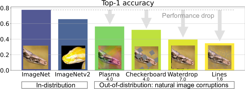
Figure 4: Top-1 accuracy of ResNet50 on in-distribution data sets (ImageNet and ImageNetv2[36]) and out-of-distribution datasets (ImageNet-$\overline{\mbox{C}}$ ). The resilience of ResNet50 drops significantly against natural corruptions.

Observations to Figure 4: Different corruptions have different effects on the model performance, and a typical “good” classifier with accuracy close to 80% can have a tremendous performance decrease in situations where a human would probably not.

4.2 Diversity of ensembles from heterogeneous architectures

To understand the diversity/accuracy trade-off of the attribution-based metric in comparison to the established prediction-based diversity approach we perform two different experiments: First, we create multiple ensembles of independently trained models with a wide diversity in architecture. Second, we create multiple ensembles using models discovered in a weight-sharing super-network [4], i.e., models whose architecture has been found using neural architecture search (NAS) and not by manual design.

The architectures explored here are CNNs (ResNext [46] & SqueezeNet [17]), Vision transformers (DeiT [44]) and NAS (MNASNET [42] & BootstrapNAS [29]) using supervised or self-supervised training. In total 14 models were trained with different hyperparameters to create three-member ensembles of all possible combinations.

Figure 5 shows the ensemble performance of all 364 ensembles created from these 14 models using an averaging consensus mechanism, i.e., the logit output of all ensemble members is averaged first and then the highest score is used to make the prediction. The left-hand side shows on the X-axis the attribution-based diversity metric (Eq. 7). The right-hand side shows the disagreement prediction diversity metric (Eq. 4). Each point is an ensemble evaluated on the entire validation dataset of ImageNet. The color indicates the final average accuracy of the ensemble. The Y-axis indicates the average benefit of creating an ensemble: $Y=A_{ens}-A_{top}$, where $A_{ens}$ is the ensemble accuracy and $A_{top}$ is the accuracy of its most accurate member, i.e., how much accuracy improvement was obtained in comparison to a single model (the most accurate in the ensemble). In this way, it can be appreciated when an ensemble makes sense: it has to lay above the zero line (dashed). The ensemble cost is measured by the number of parameters which has a direct influence on the memory and the number of operations required. The ideal ensemble is one with the brightest color, smallest radius, and residing above zero.

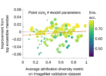
(a) Attribution diversity

(b) Prediction disagreement

Figure 5: Evaluation on ImageNet validation dataset of 364 three-member ensembles from heterogeneous architectures using averaging as consensus mechanism. Y-axis: Improvement of the ensemble against its own top ensemble member. X-axis: Normalized diversity metric. Color: absolute ensemble accuracy. Bubble size: Model parameter size. The attribution diversity metric is not negatively correlated with the ensemble improvement as disagreement diversity is.

Observations to Figure 5: The figure shows how attribution diversity is positively correlated with ensemble improvement, while it corroborates the known fact that prediction-based diversity is negatively correlated [21].

Figure 6 shows the same ensemble combinations, but this time using a majority voting consensus mechanism, i.e., the prediction with the highest number of votes wins. Draws are randomly resolved.

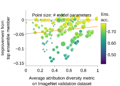
(a) Attribution diversity

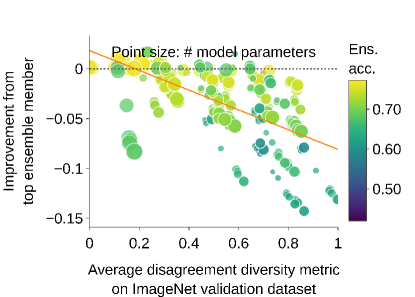
(b) Prediction disagreement

Figure 6: Evaluation on ImageNet validation dataset of the same ensembles as in Figure 5 but using voting as consensus mechanism. In contrast to averaging, voting produces mostly ensembles that decrease the final performance instead of improving it.

Observations to Figure 6: The same correlation trends can be observed with majority voting. However, the most interesting aspect is that the vast majority of the ensembles here reside under the zero line. This means that majority voting with three ensembles tends on average to produce less accurate models. This corroborates the findings of [21].

We evaluate the same ensembles on five more validation datasets and verify that the observed trend in the validation dataset applies to natural corruptions. In addition, we compare the two diversity metrics to a simple validation accuracy metric. See Figure 7.

(a) Attr. ImageNetv2

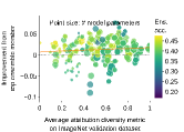
(b) Attr. Waterdrop

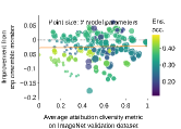
(c) Attr. Lines

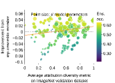
(d) Attr. Plasma

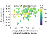
(e) Attr. Checkerb.

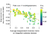
(f) Disagr. ImageNetv2

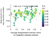
(g) Disagr. Waterdrop

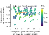
(h) Disagr. Lines

(i) Disagr. Plasma

(j) Disagr. Checkerb.

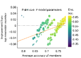
(k) Acc. ImageNetv2

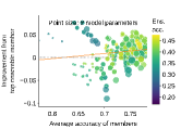
(l) Acc. Waterdrop

(m) Acc. Lines

(n) Acc. Plasma

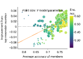
(o) Acc. Checkerb.

Figure 7: Comparison of trend lines, i.e., correlation of improvement to three different metrics on five validation datasets (consensus: averaging). Columns: Datasets. Rows: Metrics. The attribution metric (a to e) has a much lower accuracy trade-off compared to the disagreement metric (f to j) but is higher than the average accuracy metric (k to o). Bigger plots to appreciate individual ensembles are presented in Section A.2 of the supplemental material.

Observations to Figure 7: Attribution-based diversity is better correlated as well. These results serve as evidence to confirm that the diversity-accuracy trade-off is better for attribution than for prediction diversity. However, the metric of averaging the individual accuracies of the ensemble members is more strongly correlated with the ensemble improvement in corruptions.

Next, Figure 8 presents the results of the second experiment on architectures created with NAS. We used the open-source framework BootstrapNAS [29, 30] to create a weight-sharing super-network. The super-network is trained from an initial ResNet50 model. We then sample 11 subnetworks with different configurations but similar complexity by varying the width and depth of the CNN.

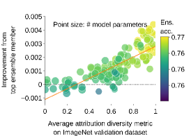
(a) Attribution

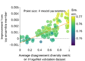
(b) Disagreement

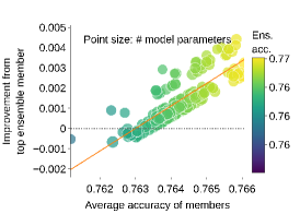
(c) Accuracy

Figure 8: Comparison of 165 heterogeneous ensembles of architectures automatically created with weight-sharing neural architecture search (NAS). 11 models with different architectures were selected to be very close in complexity, i.e., number of parameters. The correlation between the two diversity metrics is highly positive but the increment in performance is very small.

Observations to Figure 8: Although the correlations seem strong for all metrics, the actual ensemble improvement is very low, i.e., less than 0.04%.

To identify the effect of the complexity of the chosen attribution method, we evaluated the pair-wise diversity on the entire validation set on six subnetworks using Saliency and Integrated Gradients attribution methods using 1, 2, 10, and 50 backpropagation passes. See Figure 9. The average correlation coefficient of the normalized diversity scores of all methods is 0.998. Using Saliency-based attribution is then justified as it provides the lowest performance penalty as the computational overhead grows linearly with the number of backpropagation passes.

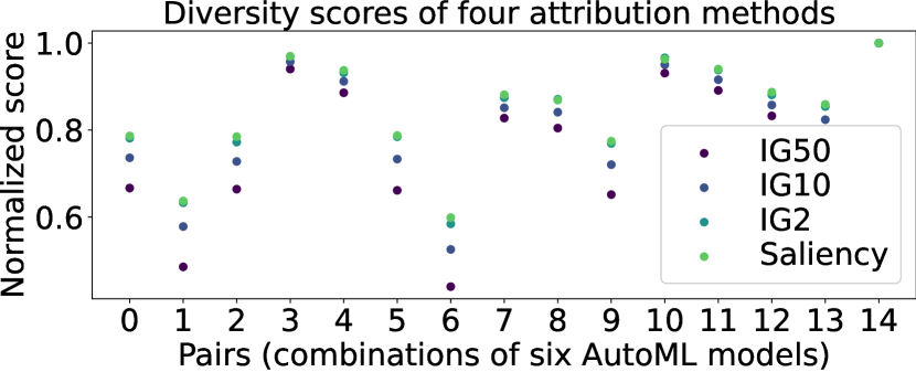
Figure 9: Comparison of Saliency and Integrated Gradients with 2, 10 & 50 samples. The X-axis represents different pairs of models created with BootstrapNAS. The Y-axis is the normalized diversity score of each method.

4.3 Enforcing diversity in homogeneous ensembles

We perform a set of training experiments to enforce diversity into the ensembles through the loss function via the Negative Correlation Learning paradigm. We use ResNet50 for all ensemble members, and evaluate different heuristics:
a) Independently trained members using cross-entropy as loss in Equation 1. Four different consensus approaches in GNCL using Equation 2: b) average, c) median, d) geometric mean, e) majority vote, f) GNCL and averaging consensus but masking the penalty term for incorrect classifications, i.e., $(h^{i}\neq y)\Rightarrow(\lambda=0)$, and g) Balancing a loss function between the team and individual members (Equation 3). The optimization method in all cases was AdaBelief [49] for 100 epochs with a learning rate of 1e-3 decaying 10% every 30 epochs, epsilon of 1e-8, betas: (0.9,0.999), batch size of 64 and a $\lambda$ factor of 0.2. In ImageNet classification, we empirically observed that bigger $\lambda$ values in Equation 2 fail to learn. Results for the six heuristics are presented in Figure 10.

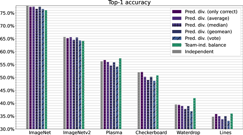
Figure 10: The resulting accuracy and resiliency to natural corruptions of diversity enforcement based on Negative Correlation Learning with different consensus mechanisms. Each ensemble has three members with a ResNet50 architecture. The heuristic of balancing the loss of the ensemble and the loss of the individual member produced the most resilient ensemble to corruptions.

Observations to Figure 10: Explicit enforcement of prediction diversity does not result in improved resilience. However the balanced loss (Eq. 3) provides a significant advantage in 3 out of 4 natural corruptions.

4.3.1 First attempt at enforcing attribution diversity

We perform a first attempt to enforce attribution diversity using the loss of Equation 8 and the same optimization parameters used in GNCL. The computational overhead to calculate the attributions is 2x using the Saliency method. Empirically, we tried five different lambda weights values: {10, 1,0.1,0.01,0.001} but found training instabilities. The smallest $\lambda$ value resulted in convergence up to epoch 21 for 63.7% top1 accuracy. We believe that the penalty term of Eq. 8 is in conflict with the original loss and it would be more appropriate to investigate a better penalty term than to optimize this hyper-parameter in future work.

4.3.2 Diversity of NCL ensembles

Figures 11, 12 together with Table 2 show three types of diversity (attribution, prediction, and intermediate representation) for three models created through independently created heterogeneous architectures, prediction diversity enforcement and attribution diversity enforcement with the following top1 accuracies on the ImageNet validation dataset: 78.2%, 76.1%, and 63.7%.

Prediction diversity. In Table 2, the Shannon equitability index metric (Eq. 5) is shown for correctly and incorrectly classified samples for three ensembles: attribution diversity (Eq. 8), prediction diversity (Eq. 4) and heterogeneous architectures on all six datasets. The heterogeneous ensemble produces more diverse predictions in general.

Table 2: Diversity of predictions from all members of three ensembles as measured by the Shanon equitability index $H$. $H_{corr}$ and $H_{inco}$ indicate the metric computed on all samples that were correctly or incorrectly classified. The six subcolumns correspond to the six validation datasets.

	$H_{corr}$						$H_{inco}$
	IN	I2	WD	LI	PL	CB	IN	I2	WD	LI	PL	CB
Att. div.	0.13	0.16	0.29	0.32	0.23	0.23	0.46	0.49	0.62	0.60	0.57	0.58
Pred. div.	0.10	0.13	0.29	0.31	0.21	0.23	0.46	0.49	0.67	0.69	0.59	0.63
Hetero.	0.12	0.17	0.35	0.37	0.25	0.29	0.51	0.55	0.74	0.77	0.67	0.71

Attribution diversity. We present a few resulting attribution maps in Figure 11 for the NCL-based prediction-diversity enforcement, attribution-diversity enforcement (at epoch 21), and independently trained architectures.

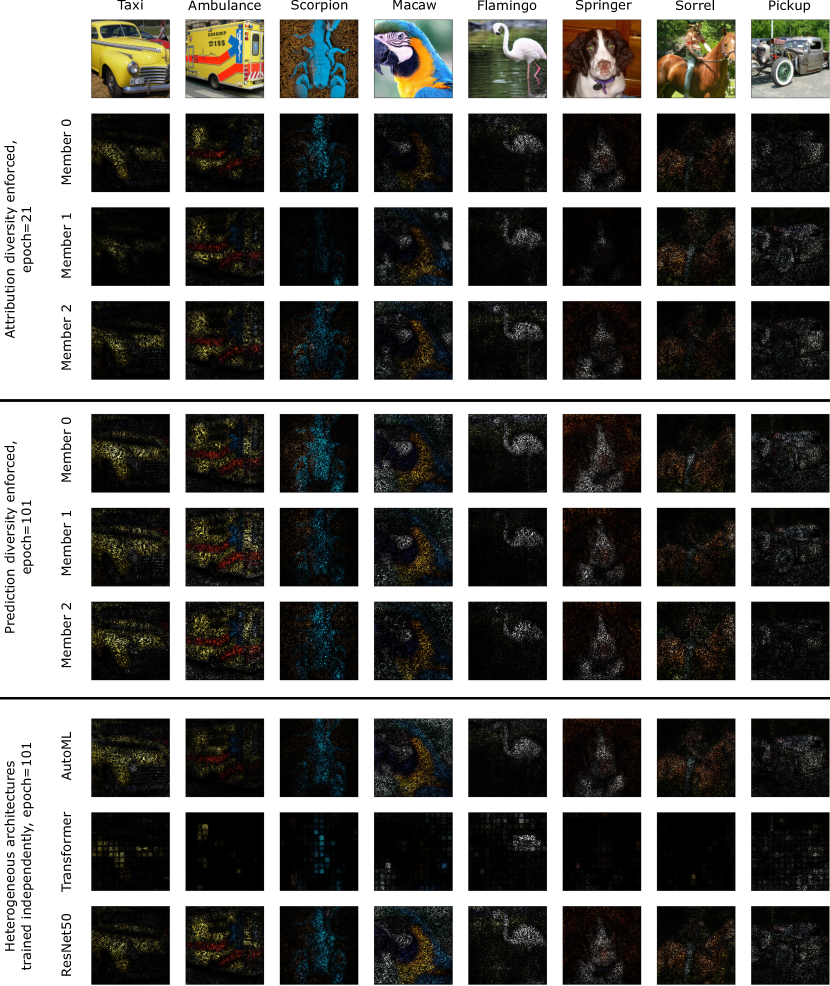
Figure 11: Attribution map diversity of different diversity-inducing techniques on 8 ImageNet val. dataset samples.

Observations to Figure 11: Independently trained heterogeneous architectures and attribution-diversity enforcement produce more diverse attribution maps than homogeneous models trained to have diverse prediction outcomes.

Representation diversity. In Figure 12, we investigate the resulting diversity/similarity of the internal layers via CKA (Equation 6) of two ensemble members for three different diversity enforcing techniques.

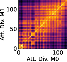
(a) Attribution diversity enf.

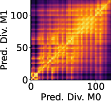
(b) Prediction diversity enf.

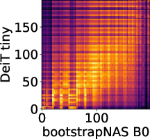
(c) Heterog. architectures

Figure 12: Centered Kernel Alignment maps to visualize the resulting similarity of model layers on different diversity enforcing techniques.

Observations to Figure 12: The CKA visualization reflects that the enforcement of attribution diversity produces less similarity in the layers than output diversity enforcement or by independent heterogeneous architectures.

5 Discussion and conclusions

In this section, we discuss and interpret the results of Section 4 and summarize the research questions’ answers.

5.1 Answers to research questions

RQ1.2: In our experiments, it is observed that model architecture is more important to resiliency than model accuracy or size. On RQ1.2, we consistently observed that attribution-based diversity is more positively correlated with accuracy than prediction-based disagreement diversity. Answering RQ1.2, balancing the loss of the individual members and the ensemble provided a significant advantage in 3 out of 4 natural corruptions when compared to the prediction diversity enforcement variants. RQ1.2: Prediction diversity was higher for heterogeneous architectures trained independently than NCL on prediction or attribution diversity. Attribution diversity is significantly lower when enforcing prediction diversity compared to heterogeneous architectures trained independently. Activation diversity is low at the last layers for both prediction and attribution diversity enforcement, while for heterogeneous architectures trained independently, the middle layers showed less diversity.

5.2 Results discussions

Advantage of Transformers vs CNNs: The superiority of the transformer architecture in terms of resilience against natural corruptions could be attributed to their capability to pay attention globally instead of locally as CNNs do, and thus they may be able to construct more useful intermediate representations that suffer less from perturbations.

NAS ensembles in our experiments are not diverse enough: Only small improvements are obtained from ensembles created from sub-networks. These are jointly trained as part of a single weight-sharing super-network and thus have little diversity. Larger search/design spaces should be explored in future work.

Balancing member vs ensemble accuracy: Explicitly enforcing prediction diversity is outperformed by implicit enforcement through the balance of ensemble and individual accuracy (Equation 3). This could be due to the use of two less conflicting objectives than prediction diversity.

Diversity-accuracy trade-off improvement: In contrast to the disagreement metric, attribution diversity does not require models to deviate from a correct prediction. The correlation is however not very strong as models tend to find similar features for prediction, and implicit attribution deviations may be the product of imperfect learning. The enforcement of attribution diversity with the proposed loss proved however to be insufficient and better heuristics need to be explored.

Diverse architectures produced more diversity than NCL-based methods An ensemble selected from a combination of independently trained heterogeneous architectures and training approaches resulted in higher levels of diversity in prediction, attribution, and intermediate layers. However, mixing different architectures does not consistently produce good ensembles as observed in the many ensembles under the zero line in Figure 7, as a good model may not benefit from ensembling with a less good one, as their common modes are not negatively correlated.

5.3 Conclusions and next steps

In this study, we explored different approaches to measure and enforce diversity in ensembles and evaluated their impact on natural data corruption resiliency. The key takeaways are: 1) model architecture is more important for resiliency than model size or model accuracy, 2) attribution-based diversity is less negatively correlated to the ensemble accuracy than prediction-based diversity, 3) a balanced loss function of individual and ensemble accuracy creates more resilient ensembles for image natural corruptions, and 4) architecture diversity produces more diversity in all explored diversity metrics: predictions, attributions, and activations.

In addition, other valuable findings are: a) Saliency attribution can be sufficient to measure input attribution diversity, b) Ensembles created from models of similar complexity that were discovered by weight-sharing Neural Architecture Search for our experiments barely provide any accuracy improvement, and c) Enforcing attribution-based diversity during training through a variance-based penalty term is not stable and needs further research.

In future work, several experiments could be done to understand the complexity-resiliency trade-off, e.g., through knowledge distillation, improved heuristics to enforce attribution diversity, and compare diversity approaches in tasks beyond image classification.

Acknowledgements

This work was partially funded by the Federal Ministry for Economic Affairs and Climate Action of Germany, as part of the research project SafeWahr (Grant Number: 19A21026C).

We would also like to thank Professors Lorenzo Strigini and Peter Popov for the fruitful conversations and feedback on this work.

A Supplemental material

A.1 Training parameters for heterogeneous architectures

Table i shows the architecture and optimization hyper-parameters used for training the models used in our experiments.

id	Architecture	Optimizer	Parameters	Scheduler	Epochs	BatchSize
ResNext50_32_2	ResNext50 cardinality=32, blockWidth=2 layers=[3;4;6;3], dropout=0.2	SGD	lr=0.1 decay=0.0001, momentum=0.9	Step: $\gamma$=0.1, epochs=30	100	32
ResNext50_32_4l	ResNext50 cardinality=32, blockWidth=4 layers=[2;2;3;2], dropout=0.2	SGD	lr=0.1 decay=0.0001, momentum=0.9	Step: $\gamma$=0.1, epochs=30	100	32
ResNext50_16_4	ResNext50 cardinality=16, blockWidth=4 layers=[3;4;6;3], dropout=0.2	SGD	lr=0.1 decay=0.0001, momentum=0.9	Step: $\gamma$=0.1, epochs=30	100	32
MNASNET_1	MNASNET ratio=1, dropout=0.2	SGD	lr=0.1 decay=0.0001, momentum=0.9	Step: $\gamma$=0.1, epochs=30	100	32
MNASNET_1p	MNASNET ratio=1, dropout=0.2	RMSprop	lr=0.256, decay=0.9, momentum=0.9	Step: $\gamma$=0.97, epochs=2.4	100	32
Squeezenet_512	Squeezenet version=1.1	SGD	lr=0.01 decay=0.0002, momentum=0.9	Step: $\gamma$=0.1, epochs=30	100	512
Squeezenet	Squeezenet version=1.1	SGD	lr=0.01 decay=0.0002, momentum=0.9	Step: $\gamma$=0.1, epochs=30	100	128
bootstrapNAS-B_0	ResNet50 depth=[0, 0, 0, 0, 1], width=[0, 0, 0, 2, 2, 2]	SGD	See Listing 1	-	-	-
	expansion=[0.2, 0.2, 0.2, 0.25, 0.2, 0.25, 0.25, 0.25,0.2, 0.25, 0.25, 0.25]
bootstrapNAS-B_1	ResNet50 d=[0, 0, 0, 0, 1], w=[0, 0, 0, 2, 2, 2]	SGD	See Listing 1	-	-	-
	expansion=[0.25, 0.2, 0.25, 0.25, 0.2, 0.25, 0.25, 0.25, 0.2, 0.25, 0.25, 0.25]
deit_tiny_p16_224	DeiT size=tiny(3 heads), patchSize=16, embedding=192	AdamW	lr=0.0005	Cosine	300	256
dino_deit_tiny1	DINO DeiT size=tiny, patchSize=16, embedding=192,	AdamW	lr=0.0005	Cosine	Backbone=300	256
	seed=0, localCropsScale={0.05,0.2}, globalCropsScale={0.4, 1.}				Classifier=100
dino_deit_tiny2	DINO DeiT size=tiny, patchSize=16, embedding=192,	AdamW	lr=0.0005	Cosine	Backbone=300	256
	seed=7, localCropsScale={0.05,0.2}, globalCropsScale={0.4, 1.}				Classifier=100
dino_resnet1	DINO ResNet50 backboneSeed=7 localCropsScale={0.05,0.14}	SGD	decay=0.0001, lr=0.03	-	Backbone=300	256
	globalCropsScale={0.14, 1.}, classifierSeed=5				Classifier=100
dino_resnet2	DINO ResNet50 backboneSeed=7 localCropsScale={0.05,0.14}	SGD	decay=0.0001, lr=0.03	-	Backbone=300	256
	globalCropsScale={0.14, 1.}, classifierSeed=15				Classifier=100

Table i: Training architectures and parameters used to create ensembles of heterogeneous architectures

Listing 1 shows an example configuration file to create a super-network using a pre-trained model from Torchvision. The configuration parameters are used by BootstrapNAS in the Neural Network Compression Framework (NNCF) and specify the size and elasticity of the super-network. Once the super-network has been trained, the user can extract models of different sizes and performances.

Listing 1: Super-network configuration example for NNCF’s BootstrapNAS

⬇

1# Insert here model and dataset fields

2# Insert here optimizer fields

3"bootstrapNAS":{

4 "training": {

5 "algorithm":"progressive_shrinking",

6 "progressivity_of_elasticity": ["depth", "width"],

7 "batchnorm_adaptation": {

8 "num_bn_adaptation_samples": 1500},

9 "schedule": {

10 "list_stage_descriptions": [

11 {"train_dims": ["depth"], "epochs": 25,

12 "depth_indicator": 1, "init_lr": 2.5e-6,

13 "epochs_lr": 25},

14 {"train_dims": ["depth"], "epochs": 40, "depth_indicator": 2, "init_lr": 2.5e-6, "epochs_lr": 40},

15 {"train_dims": ["depth", "width"], "epochs": 50, "depth_indicator": 2, "reorg_weights": true, "width_indicator": 2, "bn_adapt": true, "init_lr": 2.5e-6, "epochs_lr": 50},

16 {"train_dims": ["depth", "width"], "epochs": 50, "depth_indicator": 2, "reorg_weights": true, "width_indicator": 3, "bn_adapt": true, "init_lr": 2.5e-6, "epochs_lr": 50}

17 ]

18 },

19 "elasticity": {

20 "available_elasticity_dims": ["width", "depth"],

21 "width": {

22 "max_num_widths": 3,

23 "min_width": 32,

24 "width_step": 32,

25 "width_multipliers": [1, 0.80, 0.60]

26 }

27 }

28},

29 "search": {

30 "algorithm": "NSGA2",

31 "num_evals": 1000,

32 "population": 50,

33 "ref_acc": 93.65

34 }

35}

The parameters shown in Table ii indicate the configuration of the subnetworks extracted from the super-network in our experiments. We used a previous version of BootstrapNAS in our experiments, which extends Once-for-all (OFA) super-networks from Cai et al. [4] and follows its conventions to describe the search space. In newer versions of BootstrapNAS, expansion ratios are handled by an elastic width handler, and the search space description follows a different convention.

id	Subnetwork Configurations
B_0	depth: [0, 0, 0, 0, 1], expansion: [0.2, 0.2, 0.2, 0.25, 0.2, 0.25, 0.25, 0.25, 0.2, 0.25, 0.25, 0.25], width: [0, 0, 0, 2, 2, 2],
nB_0	depth: [0, 0, 0, 0, 1], expansion: [0.2, 0.2, 0.2, 0.25, 0.2, 0.25, 0.25, 0.25, 0.2, 0.25, 0.25, 0.25], width : [0, 0, 0, 2, 2, 2]
nB_1	depth: [0, 0, 0, 0, 1], expansion: [0.25, 0.2, 0.25, 0.25, 0.2, 0.25, 0.25, 0.25, 0.2, 0.25, 0.25, 0.25], width : [0, 0, 0, 2, 2, 2]
nB_2	depth: [0, 0, 0, 0, 1], expansion: [0.25, 0.2, 0.25, 0.2, 0.2, 0.25, 0.25, 0.25, 0.2, 0.25, 0.25, 0.25], width : [0, 0, 0, 2, 2, 2]
nB_3	depth: [0, 0, 0, 0, 1], expansion: [0.25, 0.2, 0.25, 0.25, 0.2, 0.2, 0.25, 0.25, 0.2, 0.25, 0.25, 0.25], width : [0, 0, 0, 2, 2, 2]
dB_1a	depth: [0, 0, 1, 0, 0], expansion: [0.25, 0.2, 0.25, 0.25, 0.2, 0.25, 0.25, 0.25, 0.2, 0.25, 0.25, 0.25], width : [0, 0, 0, 2, 2, 2]
dB_1b	depth: [1, 0, 0, 0, 0], expansion: [0.25, 0.2, 0.25, 0.25, 0.2, 0.25, 0.25, 0.25, 0.2, 0.25, 0.25, 0.25], width : [0, 0, 0, 2, 2, 2],
wB_1a	depth: [0, 0, 0, 0, 1], expansion: [0.25, 0.2, 0.25, 0.25, 0.2, 0.25, 0.25, 0.25, 0.2, 0.25, 0.25, 0.25], width : [0, 0, 1, 1, 2, 2],
wB_1b	depth: [0, 0, 0, 0, 1], expansion: [0.25, 0.2, 0.25, 0.25, 0.2, 0.25, 0.25, 0.25, 0.2, 0.25, 0.25, 0.25], width : [0, 1, 1, 1, 1, 2],
wB_1c	depth: [0, 0, 0, 0, 1], expansion: [0.25, 0.2, 0.25, 0.25, 0.2, 0.25, 0.25, 0.25, 0.2, 0.25, 0.25, 0.25], width : [1, 1, 1, 1, 1, 1],

Table ii: Configuration of subnetworks extracted for the creation of ensembles of heterogeneous architectures

Table iii shows the transformations used during training for all individual models.

Transform	Parameters
RandomResizedCrop	size=(224, 224), scale=(0.08, 1.0), ratio=(0.75, 1.3333), interpolation=bilinear
RandomHorizontalFlip	p=0.5
Normalize	mean=[0.485, 0.456, 0.406], std=[0.229, 0.224, 0.225]

Table iii: Training data set transforms used for the training of all models

Figure A shows the final top1 accuracy scores of each model defined by Table i.

Model id	Top 1% accuracy
ResNext50_32_2	75.198
ResNext50_32_4l	75.072
ResNext50_16_4	75.432
MNASNET_1	54.408
MNASNET_1p	54.0
Squeezenet_512	41.918
Squeezenet	56.558
bootstrapNAS-B_0	76.342
bootstrapNAS-B_1	76.282
deit_tiny_p16_224	71.654
dino_deit_tiny1	67.932
dino_deit_tiny2	67.52
dino_resnet1	67.236
dino_resnet2	67.216

Model id	Top 1% accuracy
B_0	76.342
B_1	76.282
nB_0	76.301
nB_1	76.318
nB_2	76.191
nB_3	76.142
dB_1a	76.138
dB_1b	76.084
wB_1a	76.170
wB_1b	75.804
wB_1c	75.852

Figure A: Individual accuracies of individual trained models on ImageNet validation dataset

A.2 Comparison of prediction-based disagreement, input attribution diversity and average accuracy metrics in ensembles of heterogeneous architectures

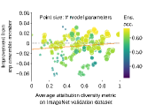
(a) Attr. ImageNetv2

(b) Attr. Waterdrop

(c) Attr. Lines

(d) Attr. Plasma

(e) Attr. Checkerb.

(f) Disagr. ImageNetv2

(g) Disagr. Waterdrop

(h) Disagr. Lines

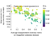
(i) Disagr. Plasma

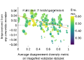
(j) Disagr. Checkerb.

(k) Acc. ImageNetv2

(l) Acc. Waterdrop

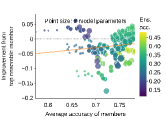
(m) Acc. Lines

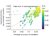
(n) Acc. Plasma

(o) Acc. Checkerb.

Figure B: Comparison of improvement correlation of three different metrics on five validation datasets using averaging as consensus mechanism. Columns: Datasets. Rows: Metrics.

References

- [1] Leo Breiman. Bagging predictors. Machine learning, 24:123–140, 1996.
- [2] Gavin Brown, Jeremy L. Wyatt, Rachel Harris, and Xin Yao. Diversity creation methods: a survey and categorisation. Inf. Fusion, 6(1):5–20, 2005.
- [3] Sebastian Buschjäger, Lukas Pfahler, and Katharina Morik. Generalized negative correlation learning for deep ensembling. CoRR, abs/2011.02952, 2020.
- [4] Han Cai, Chuang Gan, Tianzhe Wang, Zhekai Zhang, and Song Han. Once-for-all: Train one network and specialize it for efficient deployment. In 8th International Conference on Learning Representations, ICLR 2020, Addis Ababa, Ethiopia, April 26-30, 2020. OpenReview.net, 2020.
- [5] Mathilde Caron, Hugo Touvron, Ishan Misra, Hervé Jégou, Julien Mairal, Piotr Bojanowski, and Armand Joulin. Emerging properties in self-supervised vision transformers. In 2021 IEEE/CVF International Conference on Computer Vision, ICCV 2021, Montreal, QC, Canada, October 10-17, 2021, pages 9630–9640. IEEE, 2021.
- [6] Abraham Chan, Niranjhana Narayanan, Arpan Gujarati, Karthik Pattabiraman, and Sathish Gopalakrishnan. Understanding the resilience of neural network ensembles against faulty training data. In 2021 IEEE 21st International Conference on Software Quality, Reliability and Security (QRS), pages 1100–1111, 2021.
- [7] Ting Chen, Simon Kornblith, Mohammad Norouzi, and Geoffrey E. Hinton. A simple framework for contrastive learning of visual representations. In Proceedings of the 37th International Conference on Machine Learning, ICML 2020, 13-18 July 2020, Virtual Event, volume 119 of Proceedings of Machine Learning Research, pages 1597–1607. PMLR, 2020.
- [8] Jia Deng, Wei Dong, Richard Socher, Li-Jia Li, Kai Li, and Li Fei-Fei. Imagenet: A large-scale hierarchical image database. In 2009 IEEE Computer Society Conference on Computer Vision and Pattern Recognition (CVPR 2009), 20-25 June 2009, Miami, Florida, USA, pages 248–255. IEEE Computer Society, 2009.
- [9] Alexey Dosovitskiy, Lucas Beyer, Alexander Kolesnikov, Dirk Weissenborn, Xiaohua Zhai, Thomas Unterthiner, Mostafa Dehghani, Matthias Minderer, Georg Heigold, Sylvain Gelly, Jakob Uszkoreit, and Neil Houlsby. An image is worth 16x16 words: Transformers for image recognition at scale. In 9th International Conference on Learning Representations, ICLR 2021, Virtual Event, Austria, May 3-7, 2021. OpenReview.net, 2021.
- [10] Nikita Dvornik, Julien Mairal, and Cordelia Schmid. Diversity with cooperation: Ensemble methods for few-shot classification. In 2019 IEEE/CVF International Conference on Computer Vision, ICCV 2019, Seoul, Korea (South), October 27 - November 2, 2019, pages 3722–3730. IEEE, 2019.
- [11] DE Eckhardt and LD Lee. A theoretical basis for the analysis of redundant software subiect to coincident errors. NASA Tech. Memo, 86369:151, 1985.
- [12] EUROCAE. Eurocae ed-12c - software considerations in airborne systems and equipment certification. Standard ED-12C, 2012.
- [13] Stanislav Fort, Huiyi Hu, and Balaji Lakshminarayanan. Deep ensembles: A loss landscape perspective. CoRR, abs/1912.02757, 2019.
- [14] Zhiqiang Gong, Ping Zhong, and Weidong Hu. Diversity in machine learning. IEEE Access, 7:64323–64350, 2019.
- [15] Ian J. Goodfellow, Jonathon Shlens, and Christian Szegedy. Explaining and harnessing adversarial examples. In Yoshua Bengio and Yann LeCun, editors, 3rd International Conference on Learning Representations, ICLR 2015, San Diego, CA, USA, May 7-9, 2015, Conference Track Proceedings, 2015.
- [16] Kaiming He, Xiangyu Zhang, Shaoqing Ren, and Jian Sun. Deep residual learning for image recognition. In 2016 IEEE Conference on Computer Vision and Pattern Recognition, CVPR 2016, Las Vegas, NV, USA, June 27-30, 2016, pages 770–778. IEEE Computer Society, 2016.
- [17] Forrest N. Iandola, Matthew W. Moskewicz, Khalid Ashraf, Song Han, William J. Dally, and Kurt Keutzer. Squeezenet: Alexnet-level accuracy with 50x fewer parameters and <1mb model size. CoRR, abs/1602.07360, 2016.
- [18] ISO. Iso26262 road vehicles – functional safety. Standard 26262, 2011.
- [19] ISO/PAS. Iso/pas 21448:2019 safety of the intended functionality. Standard 21448, 2019.
- [20] Simon Kornblith, Mohammad Norouzi, Honglak Lee, and Geoffrey E. Hinton. Similarity of neural network representations revisited. In Kamalika Chaudhuri and Ruslan Salakhutdinov, editors, Proceedings of the 36th International Conference on Machine Learning, ICML 2019, 9-15 June 2019, Long Beach, California, USA, volume 97 of Proceedings of Machine Learning Research, pages 3519–3529. PMLR, 2019.
- [21] Ludmila I. Kuncheva and Christopher J. Whitaker. Measures of diversity in classifier ensembles and their relationship with the ensemble accuracy. Mach. Learn., 51(2):181–207, 2003.
- [22] Bev Littlewood and Douglas R. Miller. Conceptual modeling of coincident failures in multiversion software. IEEE Trans. Software Eng., 15(12):1596–1614, 1989.
- [23] Bev Littlewood, Peter Popov, and Lorenzo Strigini. Modeling software design diversity: a review. ACM Computing Surveys (CSUR), 33(2):177–208, 2001.
- [24] Y. Liu and X. Yao. Ensemble learning via negative correlation. Neural Networks, 12(10):1399–1404, 1999.
- [25] Ze Liu, Han Hu, Yutong Lin, Zhuliang Yao, Zhenda Xie, Yixuan Wei, Jia Ning, Yue Cao, Zheng Zhang, Li Dong, Furu Wei, and Baining Guo. Swin transformer V2: scaling up capacity and resolution. In IEEE/CVF Conference on Computer Vision and Pattern Recognition, CVPR 2022, New Orleans, LA, USA, June 18-24, 2022, pages 11999–12009. IEEE, 2022.
- [26] Ze Liu, Yutong Lin, Yue Cao, Han Hu, Yixuan Wei, Zheng Zhang, Stephen Lin, and Baining Guo. Swin transformer: Hierarchical vision transformer using shifted windows. In 2021 IEEE/CVF International Conference on Computer Vision, ICCV 2021, Montreal, QC, Canada, October 10-17, 2021, pages 9992–10002. IEEE, 2021.
- [27] Agnieszka Mikołajczyk and Michał Grochowski. Data augmentation for improving deep learning in image classification problem. In 2018 International Interdisciplinary PhD Workshop (IIPhDW), pages 117–122, 2018.
- [28] Eric Mintun, Alexander Kirillov, and Saining Xie. On interaction between augmentations and corruptions in natural corruption robustness. In Marc’Aurelio Ranzato, Alina Beygelzimer, Yann N. Dauphin, Percy Liang, and Jennifer Wortman Vaughan, editors, Advances in Neural Information Processing Systems 34: Annual Conference on Neural Information Processing Systems 2021, NeurIPS 2021, December 6-14, 2021, virtual, pages 3571–3583, 2021.
- [29] J. Pablo Muñoz, Nikolay Lyalyushkin, Yash Akhauri, Anastasia Senina, Alexander Kozlov, and Nilesh Jain. Enabling nas with automated super-network generation. Association for the Advancement of Artificial Intelligence, 2022.
- [30] J. Pablo Muñoz, Nikolay Lyalyushkin, Chaunte Lacewell, Anastasia Senina, Daniel Cummings, Anthony Sarah, Alexander Kozlov, and Nilesh Jain. Automated super-network generation for scalable neural architecture search. In International Conference on Automated Machine Learning, pages 5–1. PMLR, 2022.
- [31] Giung Nam, Jongmin Yoon, Yoonho Lee, and Juho Lee. Diversity matters when learning from ensembles. In Marc’Aurelio Ranzato, Alina Beygelzimer, Yann N. Dauphin, Percy Liang, and Jennifer Wortman Vaughan, editors, Advances in Neural Information Processing Systems 34: Annual Conference on Neural Information Processing Systems 2021, NeurIPS 2021, December 6-14, 2021, virtual, pages 8367–8377, 2021.
- [32] Robert K Peet. Relative diversity indices. Ecology, 56(2):496–498, 1975.
- [33] Viraj Prabhu, Sriram Yenamandra, Aaditya Singh, and Judy Hoffman. Adapting self-supervised vision transformers by probing attention-conditioned masking consistency. CoRR, abs/2206.08222, 2022.
- [34] Zhongang Qi, Saeed Khorram, and Fuxin Li. Embedding deep networks into visual explanations. Artif. Intell., 292:103435, 2021.
- [35] Dhanesh Ramachandram and Graham W. Taylor. Deep multimodal learning: A survey on recent advances and trends. IEEE Signal Processing Magazine, 34(6):96–108, 2017.
- [36] Benjamin Recht, Rebecca Roelofs, Ludwig Schmidt, and Vaishaal Shankar. Do imagenet classifiers generalize to imagenet? In Kamalika Chaudhuri and Ruslan Salakhutdinov, editors, Proceedings of the 36th International Conference on Machine Learning, ICML 2019, 9-15 June 2019, Long Beach, California, USA, volume 97 of Proceedings of Machine Learning Research, pages 5389–5400. PMLR, 2019.
- [37] Robert E Schapire. A brief introduction to boosting. In Ijcai, volume 99, pages 1401–1406. Citeseer, 1999.
- [38] Florian Schroff, Dmitry Kalenichenko, and James Philbin. Facenet: A unified embedding for face recognition and clustering. In IEEE Conference on Computer Vision and Pattern Recognition, CVPR 2015, Boston, MA, USA, June 7-12, 2015, pages 815–823. IEEE Computer Society, 2015.
- [39] Ramprasaath R. Selvaraju, Michael Cogswell, Abhishek Das, Ramakrishna Vedantam, Devi Parikh, and Dhruv Batra. Grad-cam: Visual explanations from deep networks via gradient-based localization. In IEEE International Conference on Computer Vision, ICCV 2017, Venice, Italy, October 22-29, 2017, pages 618–626. IEEE Computer Society, 2017.
- [40] Karen Simonyan, Andrea Vedaldi, and Andrew Zisserman. Deep inside convolutional networks: Visualising image classification models and saliency maps. In Yoshua Bengio and Yann LeCun, editors, 2nd International Conference on Learning Representations, ICLR 2014, Banff, AB, Canada, April 14-16, 2014, Workshop Track Proceedings, 2014.
- [41] Mukund Sundararajan, Ankur Taly, and Qiqi Yan. Axiomatic attribution for deep networks. In Doina Precup and Yee Whye Teh, editors, Proceedings of the 34th International Conference on Machine Learning, ICML 2017, Sydney, NSW, Australia, 6-11 August 2017, volume 70 of Proceedings of Machine Learning Research, pages 3319–3328. PMLR, 2017.
- [42] Mingxing Tan, Bo Chen, Ruoming Pang, Vijay Vasudevan, Mark Sandler, Andrew Howard, and Quoc V. Le. Mnasnet: Platform-aware neural architecture search for mobile. In IEEE Conference on Computer Vision and Pattern Recognition, CVPR 2019, Long Beach, CA, USA, June 16-20, 2019, pages 2820–2828. Computer Vision Foundation / IEEE, 2019.
- [43] Mingxing Tan and Quoc V. Le. Efficientnet: Rethinking model scaling for convolutional neural networks. In Kamalika Chaudhuri and Ruslan Salakhutdinov, editors, Proceedings of the 36th International Conference on Machine Learning, ICML 2019, 9-15 June 2019, Long Beach, California, USA, volume 97 of Proceedings of Machine Learning Research, pages 6105–6114. PMLR, 2019.
- [44] Hugo Touvron, Matthieu Cord, Matthijs Douze, Francisco Massa, Alexandre Sablayrolles, and Hervé Jégou. Training data-efficient image transformers & distillation through attention. In Marina Meila and Tong Zhang, editors, Proceedings of the 38th International Conference on Machine Learning, ICML 2021, 18-24 July 2021, Virtual Event, volume 139 of Proceedings of Machine Learning Research, pages 10347–10357. PMLR, 2021.
- [45] Ashish Vaswani, Noam Shazeer, Niki Parmar, Jakob Uszkoreit, Llion Jones, Aidan N. Gomez, Lukasz Kaiser, and Illia Polosukhin. Attention is all you need. In Isabelle Guyon, Ulrike von Luxburg, Samy Bengio, Hanna M. Wallach, Rob Fergus, S. V. N. Vishwanathan, and Roman Garnett, editors, Advances in Neural Information Processing Systems 30: Annual Conference on Neural Information Processing Systems 2017, December 4-9, 2017, Long Beach, CA, USA, pages 5998–6008, 2017.
- [46] Saining Xie, Ross B. Girshick, Piotr Dollár, Zhuowen Tu, and Kaiming He. Aggregated residual transformations for deep neural networks. In 2017 IEEE Conference on Computer Vision and Pattern Recognition, CVPR 2017, Honolulu, HI, USA, July 21-26, 2017, pages 5987–5995. IEEE Computer Society, 2017.
- [47] Y.C. Yeh. Design considerations in boeing 777 fly-by-wire computers. In Proceedings Third IEEE International High-Assurance Systems Engineering Symposium (Cat. No.98EX231), pages 64–72, 1998.
- [48] Xiaojie Zhao, Yuming Shen, Shidong Wang, and Haofeng Zhang. Boosting generative zero-shot learning by synthesizing diverse features with attribute augmentation. In Thirty-Sixth AAAI Conference on Artificial Intelligence, AAAI 2022, Thirty-Fourth Conference on Innovative Applications of Artificial Intelligence, IAAI 2022, The Twelveth Symposium on Educational Advances in Artificial Intelligence, EAAI 2022 Virtual Event, February 22 - March 1, 2022, pages 3454–3462. AAAI Press, 2022.
- [49] Juntang Zhuang, Tommy Tang, Yifan Ding, Sekhar Tatikonda, Nicha C. Dvornek, Xenophon Papademetris, and James S. Duncan. Adabelief optimizer: Adapting stepsizes by the belief in observed gradients. In Hugo Larochelle, Marc’Aurelio Ranzato, Raia Hadsell, Maria-Florina Balcan, and Hsuan-Tien Lin, editors, Advances in Neural Information Processing Systems 33: Annual Conference on Neural Information Processing Systems 2020, NeurIPS 2020, December 6-12, 2020, virtual, 2020.