Topology optimization with physics-informed neural networks:
application to noninvasive detection of hidden geometries

Abstract

Detecting hidden geometrical structures from surface measurements under electromagnetic, acoustic, or mechanical loading is the goal of noninvasive imaging techniques in medical and industrial applications. Solving the inverse problem can be challenging due to the unknown topology and geometry, the sparsity of the data, and the complexity of the physical laws. Physics-informed neural networks (PINNs) have shown promise as a simple-yet-powerful tool for problem inversion, but they have yet to be applied to general problems with a priori unknown topology. Here, we introduce a topology optimization framework based on PINNs that solves geometry detection problems without prior knowledge of the number or types of shapes. We allow for arbitrary solution topology by representing the geometry using a material density field that approaches binary values thanks to a novel eikonal regularization. We validate our framework by detecting the number, locations, and shapes of hidden voids and inclusions in linear and nonlinear elastic bodies using measurements of outer surface displacement from a single mechanical loading experiment. Our methodology opens a pathway for PINNs to solve various engineering problems targeting geometry optimization.

Noninvasive detection of hidden geometries is desirable in countless applications including medical imaging and diagnosis [13], nondestructive evaluation of materials [28], and mine detection [49]. The goal is to infer the locations, and shapes of structures hidden inside a matrix from surface measurements of the response to an applied load such as a magnetic field [19, 22], an electric current [2], or a mechanical traction [9]. Identifying these internal boundaries from the measured data constitutes a challenging inverse problem due to the unknown topology, the large number of parameters required to describe arbitrary geometries [27], the potential sparsity of the data, and the complexity of the underlying physical laws which usually take the form of linear or nonlinear partial differential equations (PDEs) [18].

In recent years, physics-informed neural networks (PINNs) have emerged as a robust tool for problem inversion across disciplines and over a range of model complexity [16, 33, 45]. PINNs’ ability to seamlessly blend measurement data or design objectives with governing PDEs in nontrivial geometries has enabled practitioners to solve easily a range of inverse problems involving identification or design of unknown properties in fields ranging from mechanics to optics and medicine [46, 50, 36, 25, 11, 42]. Encouraged by these early successes, we introduce in this paper a general topology optimization (TO) framework to solve noninvasive geometry detection problems using PINNs, leveraging both the measurements and the governing PDEs. Building on the strength of PINNs, our approach is straightforward to implement regardless of the complexity of the physical model, produces accurate results using measurement data from a single experiment, and does not require a training dataset. To the best of our knowledge, the present work marks the first time that PINNs have been applied to problems involving a priori unknown topology and geometry.

Classical approaches to solve geometry identification inverse problems tend to be complex as they combine traditional numerical solvers such as the finite-element or boundary-element method, adjoint techniques to evaluate the sensitivity of the error residual with respect to the shape or the topology, and gradient descent-based optimization algorithms to update the geometry at every iteration [7, 20, 4, 18, 24]. Furthermore, these techniques call for carefully chosen regularization schemes and do not always yield satisfactory results, especially in the presence of sparse measurements acquired by only one or a few sets of experiments. For example, in the mechanical loading case where voids and inclusions in an elastic body are to be identified from measurements of surface displacement in response to a prescribed traction, past studies limit themselves to simple shapes like squares and circles or fail to find the right number of shapes [34, 5, 9, 39, 40]. Attempts to apply PINNs to geometry detection are in their infancy, so far restricted to cases where the number and shape-type of hidden voids or inclusions in an elastic structure are provided in advance [56].

Our PINN-based TO framework does not require any prior knowledge on the number and types of shapes. We allow for arbitrary solution topology by representing the geometry using a material density field equal to 0 in one phase and 1 in the other. The material density is parameterized through a neural network, which needs to be regularized in order to push the material density towards 0 or 1 values. Thus, one key ingredient in our framework is a novel eikonal regularization, inspired from fast-marching level-set methods [1, 43] and neural signed distance functions [23], that promotes a constant thickness of the interface region where the material density transitions between 0 and 1, leading to well-defined boundaries throughout the domain. This eikonal regularization enters as an additional term in the standard PINN loss, which is then used to train the neural networks underlying the material density and physical quantities to yield a solution to the geometry detection problem. As an illustration, we apply our framework to cases involving an elastic body under mechanical loading, and discover the topology, locations, and shapes of hidden structures for a variety of geometries and materials.

Results

Problem formulation

We consider noninvasive geometry detection problems of the following form. Suppose we have a continuous body $\mathcal{B}$ containing an unknown number of hidden voids or inclusions, with unknown shapes and at unknown locations within the body. The material properties are assumed to be known and homogeneous within the body and the inclusions. We then apply a certain type of loading (e.g. mechanical, thermal, acoustic, etc) on the body’s external boundary $\partial\mathcal{B}^{\mathrm{ext}}$, which produces a response within the body that can be described by a set of $n$ physical quantities (e.g. displacements, stresses, temperature, etc). These physical quantities can be lumped into a vector field $\boldsymbol{\psi}:\mathcal{B}\rightarrow\mathbb{R}^{n}$ and satisfy a known set of governing PDEs. The goal of the inverse problem is to identify the number, locations, and shapes of the voids or inclusions based on measurements along $\partial\mathcal{B}^{\mathrm{ext}}$ of some of the physical quantities contained in $\boldsymbol{\psi}$.

As a concrete example, we consider two prototypical plane-strain elasticity inverse problems.

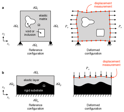
Fig. 1: Setup of two geometry identification problems in elastic bodies under mechanical loading. a, A square elastic matrix with hidden voids or inclusions is pulled by a known uniform traction on two opposite sides. The goal is to identify the number, locations, and shapes of the voids or inclusions within using measurements of the displacement occurring along the outer boundary of the matrix. b, An elastic layer on top of a hidden rigid substrate is compressed from the top by a uniform pressure. The goal is to identify the shape of the substrate using measurements of the displacement of the top surface.

In the first case, a square elastic matrix with hidden voids or inclusions is pulled by a uniform traction $P_{o}$ on two sides (Fig. 1a). The goal of the inverse problem is to identify the number, locations, and shapes of the voids or inclusions using discrete measurements of the displacement of the outer boundary of the matrix. In the second case, an elastic layer on top of a hidden rigid substrate is compressed from the top by a uniform pressure $P_{o}$, with periodic lateral boundary conditions (Fig. 1b). The goal is to identify the shape of the substrate using discrete measurements of the displacement of the top surface. For both cases, the constitutive properties of all materials are assumed to be known. We will consider two different types of constitutive laws: compressible linear elasticity, which characterizes the small deformation of any compressible elastic material, and incompressible nonlinear hyperelasticity, which models the large deformation of rubber-like materials. In the linear elastic case, there exists a unique solution to the inverse problem (see proof in Supplementary Information), making it well-suited to evaluating the accuracy of our TO framework.

Following density-based TO methods [51], we avoid any restriction on the number and shapes of hidden structures by parameterizing the geometry of the elastic body $\mathcal{B}$ through a discrete-valued material density function $\rho:\Omega\rightarrow\{0,1\}$, where $\Omega$ is a global domain comprising both $\mathcal{B}$ and the hidden voids or inclusions. The material density is defined to be equal to 1 in the elastic body $\mathcal{B}$ and 0 in the voids or inclusions. The physical quantities $\boldsymbol{\psi}$ can then be extended to the global domain $\Omega$ by introducing an explicit $\rho$-dependence in their governing PDEs, leading to equations of the form

$$\mathbf{r}(\boldsymbol{\psi}(\mathbf{x}),\rho(\mathbf{x})) =0,\quad\mathbf{x}\in\Omega,$$ (1a)

$$\mathbf{b}(\boldsymbol{\psi}(\mathbf{x})) =0,\quad\mathbf{x}\in\partial\Omega,$$ (1b)

with known boundary conditions defined solely on the external boundary $\partial\Omega=\partial\mathcal{B}^{\mathrm{ext}}$. Note that the residual functions $\mathbf{r}$ and $\mathbf{b}$ may contain partial derivatives of $\boldsymbol{\psi}$ and $\rho$. The inverse problem is now to find the distribution of material density $\rho$ in $\Omega$ so that the corresponding solution for $\boldsymbol{\psi}$ matches surface measurements $\boldsymbol{\psi}_{i}^{m}$ at discrete locations $\mathbf{x}_{i}\in\partial\Omega^{m}\subset\partial\Omega$, that is,

$$\boldsymbol{\psi}(\mathbf{x}_{i})=\boldsymbol{\psi}_{i}^{m},\quad\mathbf{x}_{i}\in\partial\Omega^{m}.$$ (2)

In practice, we might only measure select quantities in $\boldsymbol{\psi}$ at some of the locations, but we do not write so explicitly to avoid overloading the notation.

For the linear elasticity problem that we consider as an example, $\boldsymbol{\psi}=(\mathbf{u},\boldsymbol{\sigma})$ where $\mathbf{u}(\mathbf{x})$ and $\boldsymbol{\sigma}(\mathbf{x})$ are displacement and stress fields, respectively, and the governing equations comprise equilibrium relations $\sum_{j}\partial\sigma_{ij}/\partial x_{j}=0$ and a constitutive law $F(\boldsymbol{\sigma},\nabla\mathbf{u},\rho)=0$, both defined over $\Omega$. The presence of $\rho$ in the constitutive law specifies different material behaviors for the elastic solid phase and the void or rigid inclusion phase. The applied boundary conditions take the form $\mathbf{u}=\bar{\mathbf{u}}$ on $\partial\Omega_{u}$ and $\boldsymbol{\sigma}\mathbf{n}=\bar{\mathbf{t}}$ on $\partial\Omega_{t}$, where $\partial\Omega_{u}$ and $\partial\Omega_{t}$ are partitions of the external boundary with applied displacements and applied tractions, respectively, and $\mathbf{n}$ is the outward unit normal. In the case of the elastic layer, the outer boundary also comprises a portion $\partial\Omega_{p}$ with periodic boundary conditions on the displacement and traction. Finally, the requirement that the predictions for $\mathbf{u}$ at the surface match the measurement data is expressed as $\mathbf{u}(\mathbf{x}_{i})=\mathbf{u}_{i}^{m}$, $\mathbf{x}_{i}\in\partial\Omega^{m}$. See Methods for a detailed formulation of the governing equations and boundary conditions for all considered cases.

Similar to density-based TO methods [51], we relax the binary constraint on the material density by allowing intermediate values of $\rho$ between 0 and 1. This renders the problem amenable to gradient-based optimization, which underpins the PINN-based TO framework that we introduce in the next section. However, the challenge is to find an appropriate regularization mechanism that drives the optimized material distribution towards 0 and 1 rather than intermediate values devoid of physical meaning. As we will show in the discussion, common strategies employed in TO [18, 51] do not yield satisfactory results in our PINN-based framework for geometry detection problems. Thus, we have developed a novel eikonal regularization scheme inspired from level-set methods and signed distance functions, which we will describe after presenting the general framework.

General framework

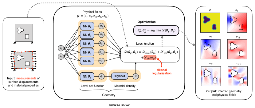
Fig. 2: TO framework for noninvasive detection of hidden geometries. The geometry of the system, which is initially unknown, is parameterized by a material density field given through a level-set function and equal to 1 in the elastic body and 0 in the voids or inclusions. The level-set function and the physical quantities describing the problem are approximated with deep neural networks designed to inherently satisfy the applied boundary conditions. These neural networks are then trained to minimize a loss function that drives the material density and physical quantities towards satisfying the governing equation of the problem while matching discrete surface measurements. A crucial eikonal regularization term in the loss function ensures that the material density transitions between 0 and 1 over a prescribed length scale and avoids settling on intermediate values. By the end of the optimization, the converged material distribution reveals the location and shapes of the hidden structures.

We propose a TO framework based on PINNs for solving noninvasive geometry detection problems (Fig. 2). At the core of the framework are several deep neural networks that approximate the physical quantities $\boldsymbol{\psi}(\mathbf{x})$ describing the problem and the material density $\rho(\mathbf{x})$. For the physical quantities, each neural network maps the spatial location $\mathbf{x}=(x_{1},x_{2})$ to one of the variables in $\boldsymbol{\psi}=(\psi_{1},\cdots,\psi_{n})$; this can be expressed as $\psi_{i}=\bar{\psi}_{i}(\mathbf{x};\boldsymbol{\theta}_{i})$ where $\bar{\psi}_{i}$ is the map defined by the $i$th neural network and its trainable parameters $\boldsymbol{\theta}_{i}$ (see Methods). For the material distribution, we first define a neural network with trainable parameters $\boldsymbol{\theta}_{\phi}$ that maps $\mathbf{x}$ to a scalar variable $\phi=\bar{\phi}(\mathbf{x};\boldsymbol{\theta}_{\phi})$. A sigmoid function is then applied to $\phi$ to yield $\rho=\mathrm{sigmoid}(\phi/\delta)=\mathrm{sigmoid}(\bar{\phi}(\mathbf{x};\boldsymbol{\theta}_{\phi})/\delta)$, which we simply write as $\rho=\bar{\rho}(\mathbf{x},\boldsymbol{\theta}_{\phi})$. This construction ensures that the material density $\rho$ remains between 0 and 1, and $\delta$ is a transition length scale that we will comment on later. We define the phase transition to occur at $\rho=0.5$ so that the zero level-set of $\phi$ delineates the boundary between the two material phases, hence $\phi$ is hereafter referred to as a level-set function [44, 43].

We now seek the parameters $\boldsymbol{\theta}_{\boldsymbol{\psi}}=\{\boldsymbol{\theta}_{1},\dots,\boldsymbol{\theta}_{n}\}$ and $\boldsymbol{\theta}_{\phi}$ so that the neural network approximations for $\boldsymbol{\psi}(\mathbf{x})$ and $\rho(\mathbf{x})$ satisfy the governing equations (1a) and applied boundary conditions (1b) while matching the surface measurements (2). This is achieved by constructing a loss function of the form

$$\mathcal{L}(\boldsymbol{\theta}_{\boldsymbol{\psi}},\boldsymbol{\theta}_{\phi}) =\lambda_{\mathrm{meas}}\mathcal{L}_{\mathrm{meas}}(\boldsymbol{\theta}_{\boldsymbol{\psi}})+\lambda_{\mathrm{gov}}\mathcal{L}_{\mathrm{gov}}(\boldsymbol{\theta}_{\boldsymbol{\psi}},\boldsymbol{\theta}_{\phi})$$

$$\quad+\lambda_{\mathrm{reg}}\mathcal{L}_{\mathrm{eik}}(\boldsymbol{\theta}_{\phi}),$$ (3)

where $\mathcal{L}_{\mathrm{meas}}$ and $\mathcal{L}_{\mathrm{gov}}$ measure the degree to which the neural network approximations do not satisfy the measurements and governing equations, respectively, $\mathcal{L}_{\mathrm{eik}}$ is a crucial regularization term that drives $\rho$ towards 0 or 1 values and that we will explain below, and the $\lambda$’s are scalar weights. The measurement loss takes the form

$$\mathcal{L}_{\mathrm{meas}}(\boldsymbol{\theta}_{\boldsymbol{\psi}})=\frac{1}{|\partial\Omega^{m}|}\sum_{\mathbf{x}_{i}\in\partial\Omega^{m}}|\bar{\boldsymbol{\psi}}(\mathbf{x}_{i};\boldsymbol{\theta}_{\boldsymbol{\psi}})-\boldsymbol{\psi}_{i}^{m}|^{2},$$ (4)

where $|\partial\Omega^{m}|$ denotes the size of the set $\partial\Omega^{m}$. A trivial modification of this expression is necessary in the case where only select quantities in $\boldsymbol{\psi}$ are measured. The governing equations loss takes the form

$$\mathcal{L}_{\mathrm{gov}}(\boldsymbol{\theta}_{\boldsymbol{\psi}},\boldsymbol{\theta}_{\phi})=\frac{1}{|\Omega^{d}|}\sum_{\mathbf{x}_{i}\in\Omega^{d}}|\mathbf{r}(\bar{\boldsymbol{\psi}}(\mathbf{x}_{i};\boldsymbol{\theta}_{\boldsymbol{\psi}}),\bar{\rho}(\mathbf{x}_{i};\boldsymbol{\theta}_{\phi}))|^{2},$$ (5)

where $\Omega^{d}$ is a set of collocation points in $\Omega$, and we use automatic differentiation to calculate in a mesh-free fashion the spatial derivatives contained in $\mathbf{r}$. We design the architecture of our neural networks in such a way that they inherently satisfy the boundary conditions (see Methods, section “Detailed PINNs formulation”).

Finally, the optimal parameters $\boldsymbol{\theta}_{\boldsymbol{\psi}}^{*}$ and $\boldsymbol{\theta}_{\phi}^{*}$ that solve the problem can be obtained by training the neural networks to minimize the loss (3) using stochastic gradient descent-based optimization. The corresponding physical quantities $\bar{\boldsymbol{\psi}}(\mathbf{x};\boldsymbol{\theta}_{\boldsymbol{\psi}}^{*})$ will match the discrete surface measurements while satisfying the governing equations of the problem, while the corresponding material density $\bar{\rho}(\mathbf{x};\boldsymbol{\theta}_{\phi}^{*})$ will reveal the number, locations, and shapes of the hidden voids or inclusions.

Material density regularization

We now describe the key ingredient that ensures the success of our framework. As mentioned above, the main challenge is to promote the material density $\rho(\mathbf{x})$ to converge towards 0 or 1 away from the material phase boundaries, given by the zero level-set $\phi=0$. Moreover, we desire the thickness of the transition region along these boundaries, where $\rho$ goes from 0 to 1, to be uniform everywhere in order to ensure consistency of physical laws across the interface (e.g. stress jumps).

To visualize what happens in the absence of regularization, consider a random instance of the neural network $\phi=\bar{\phi}(\mathbf{x},\boldsymbol{\theta}_{\phi})$ (Fig. 3a, left) and the corresponding material distribution $\rho=\mathrm{sigmoid}(\phi/\delta)$ with $\delta=0.01$ (Fig. 3a, center).

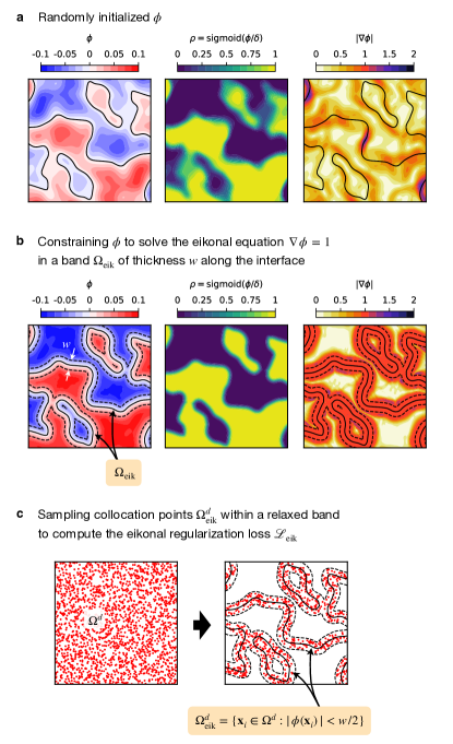
Fig. 3: Eikonal regularization of the material density. $\mathbf{a}$, A random level-set function $\phi$ yields a material density $\rho=\mathrm{sigmoid}(\phi/\delta)$ with large regions of values between 0 and 1, due to the nonuniformity of the gradient $|\nabla\phi|$ along the material boundaries defined by the zero level-set of $\phi$ (black lines). $\mathbf{b}$, Constraining $\phi$ to solve the eikonal equation $\nabla\phi=1$ in a narrow band $\Omega_{\mathrm{eik}}$ of thickness $w$ (edges depicted by dashed lines) along the material boundaries results in a uniform transition thickness of $\rho$ from 0 to 1, without large regions of intermediate density values. $\mathbf{c}$, The loss $\mathcal{L}_{\mathrm{eik}}$ implements the eikonal regularization in the PINN-based TO framework by penalizing deviations away from the constraint $|\nabla\phi|=1$ on a subset of collocation points $\Omega_{\mathrm{eik}}^{d}\subset\Omega_{d}$ that approximates the true narrow band $\Omega_{\mathrm{eik}}$.

The sigmoid transformation ensures that $\rho$ never drops below 0 or exceeds 1, leading to large regions corresponding to one phase or the other. However, the thickness of the transition region where $\rho$ goes from 0 to 1 is not everywhere uniform, resulting in large zones where $\rho$ assumes nonphysical values between 0 and 1 (Fig. 3a, center). This behavior stems from the non-uniformity of the gradient norm $|\nabla\phi|$ along the material boundaries $\phi=0$, with small and large values of $|\nabla\phi|$ leading to wide and narrow transition regions, respectively (Fig. 3a, right).

We propose to regularize the material density by forcing the gradient norm $|\nabla\phi|$ to be unity in a narrow band $\Omega_{\mathrm{eik}}$ of width $w$ along the material boundaries defined by the zero level-set $\phi=0$. In this way, $\phi$ becomes a signed distance function to the material boundary in the narrow band, thereby constraining the gradient of $\rho$ to be constant along the interface. To ensure that the narrow band covers the near-entirety of the transition region where $\rho$ goes from 0 to 1, we choose $w=10\delta$ so that $\rho=\mathrm{sigmoid}(\pm w/2\delta)=\mathrm{sigmoid}(\pm 5)\simeq 0$ or $1$ along the edge of the narrow band. To illustrate the effect of such regularization, we consider the previous random instance of the neural network $\phi=\bar{\phi}(\mathbf{x},\boldsymbol{\theta}_{\phi})$ and enforce the constraint $|\nabla\phi|=1$ in the narrow band $\Omega_{\mathrm{eik}}$ along its zero level-set (Fig. 3b, left and right). The zero level-set is kept fixed to facilitate comparison with the unregularized case (Fig. 3a). With $\phi$ now behaving like a signed-distance function in the narrow band, a uniform transition thickness for $\rho$ along all material boundaries is achieved, without large regions of intermediate density values (Fig. 3b, center).

In practice, we implement this regularization into our PINN-based TO framework by including an ‘eikonal’ loss term $\mathcal{L}_{\mathrm{eik}}$ in (3), which takes the form

$$\mathcal{L}_{\mathrm{eik}}(\boldsymbol{\theta}_{\phi})=\frac{1}{|\Omega_{\mathrm{eik}}^{d}|}\sum_{\mathbf{x}_{i}\in\Omega_{\mathrm{eik}}^{d}}\left(|\nabla\phi(\mathbf{x}_{i})|-1\right)^{2},$$ (6)

where $\Omega_{\mathrm{eik}}^{d}=\{\mathbf{x}_{i}\in\Omega^{d}:|\phi(\mathbf{x}_{i})|<w/2\}$. The aim of this term is to penalize deviations away from the constraint $|\nabla\phi|=1$ in the narrow band $\Omega_{\mathrm{eik}}$ of width $w$ along the interface defined by the zero level-set $\phi=0$. Because finding the subset of collocation points $\mathbf{x}_{i}$ in $\Omega^{d}$ belonging to the true narrow band of width $w$ at every step of the training process would be too expensive, we instead relax the domain over which the constraint $|\nabla\phi|=1$ is active by utilizing the subset $\Omega_{\mathrm{eik}}^{d}$ of collocation points that satisfy $|\phi(\mathbf{x}_{i})|<w/2$. As the constraint $|\nabla\phi|=1$ is progressively better satisfied during the training process, $\Omega_{\mathrm{eik}}^{d}$ will eventually overlap the true narrow band of width $w$ along the zero level-set of $\phi$ (Fig. 3c).

Since the constraint $|\nabla\phi|=1$ in the narrow band takes the form of an eikonal equation, we call this approach eikonal regularization. We emphasize that in contrast to recent works training neural networks to solve the eikonal equation [23], our eikonal regularization does not force $\phi$ to vanish on a predefined boundary. Rather, the zero level-set of $\phi$ evolves freely during the training process in such a way that the corresponding material distribution $\rho=\mathrm{sigmoid}(\phi/\delta)$ and physical quantities $\boldsymbol{\psi}$ minimize the total loss (3), eventually revealing the material boundaries delineating the hidden voids or inclusions.

Setup of numerical experiments

We evaluate our TO framework on a range of challenging test cases involving different numbers and shapes of hidden structures and various materials (Methods, Tabs. 1 and 2). As a substitute for real experiments, we use the finite-element method (FEM) software Abaqus to compute the deformed shape of the boundary of the elastic structure and generate the measurement data for each case (Methods, section “FEM simulations”). Using this measurement data, we run our TO framework to discover the number, locations, and shapes of the hidden voids or rigid inclusions (for implementation and training details, see Methods, section “Architecture and training details”). We then compare the obtained results with the ground truth — the voids or inclusions originally fed into Abaqus — to assess the efficacy of our framework.

Elastic matrix experiments

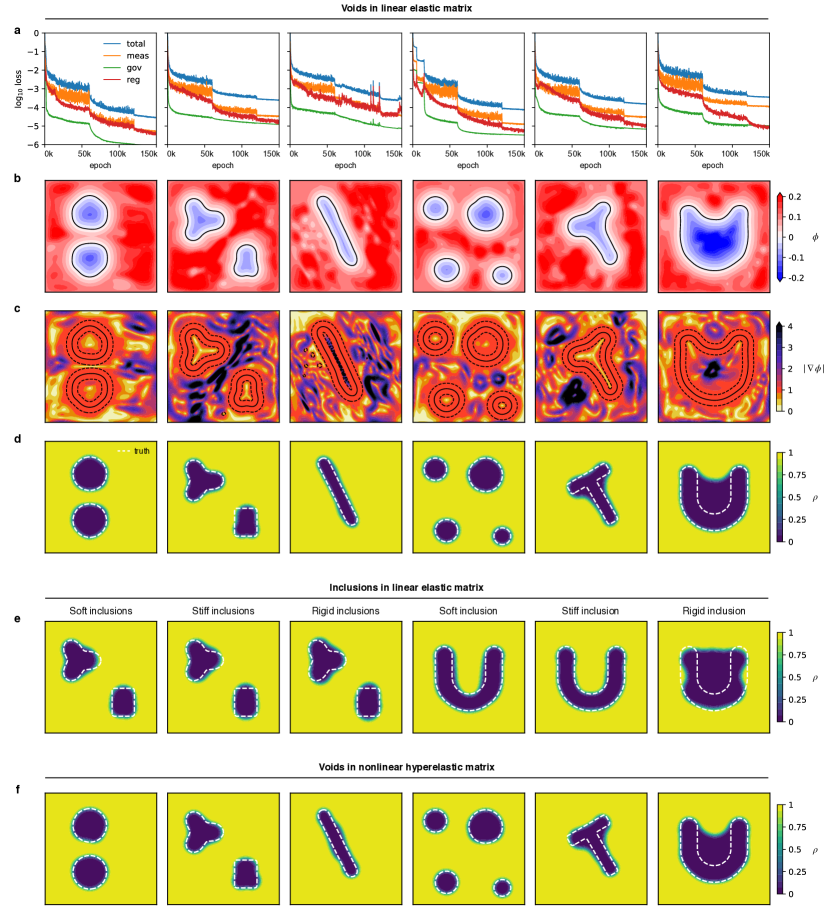
Fig. 4: Identification of voids and inclusions in elastic matrices. A linear elastic matrix containing voids (a-d): a, The various loss components that enforce the solution to match the surface measurement data, satisfy the governing equations, and obey the eikonal regularization, are being minimized during the training process. b,c, The final level-set function $\phi$ and its gradient magnitude $|\nabla\phi|$ show the effect of the eikonal regularization, making $\phi$ a signed distance function in narrow band along the interface. d, The final material density $\rho$ reveals the number, locations, and shapes of the hidden voids, which are compared with the ground truth shown in dotted white lines. e, The final material density predictions in the case of a linear elastic matrix containing soft, stiff or rigid inclusions. f, The final material density predictions in the case of a nonlinear hyperelastic matrix containing voids subject to large stretches.

We first apply our framework to cases involving a linear elastic matrix (Fig. 1a) containing voids (cases 1, 3, 8, 10, 15, 17 in Methods, Tab. 1). As the various loss components are minimized during training (Fig. 4a), the material density $\rho$ evolves and splits in a way that progressively reveals the number, locations, and shapes of the hidden voids (Extended Data Fig. 1 and Supplementary Movie 1), without advance knowledge of their topology. By the end of the training, the transition regions where the material density goes from 0 to 1 have uniform thickness along all internal boundaries (Fig. 4d), thanks to the eikonal regularization that encourages the level-set gradient $\nabla\phi$ to have unit norm in a band along the material boundaries $\phi=0$ (Fig. 4b,c). The agreement between the final inferred shapes and the ground truth is remarkable, with our framework able to recover intricate details such as the three lobes and the concave surfaces of the star-shaped void (Fig. 4d, second from left), or the exact aspect ratio and location of a thin slit (Fig. 4d, third from left). The stress and strain fields of the deformed matrix are also obtained as a byproduct of the solution process (Extended Data Fig. 2). The only case that is not completely identified is the U-shaped void (Fig. 4d, first from right), a result of the miniscule influence of the inner lobe on the outer surface displacements due to its low level of strain and stress (Extended Data Fig. 8). Finally, our framework maintains accurate results when reducing the number of surface measurement points or restricting measurements to a few surfaces (Extended Data Figs. 5-7).

Next, we consider cases involving linear elastic and rigid inclusions in the linear elastic matrix (cases 4, 5, 6, 11, 12, 13 in Methods, Tab. 1). Our framework successfully identifies the inclusions in almost all cases (Fig. 4e). Inferred displacements and stresses of the deformed matrix (Extended Data Fig. 3) confirm the intuition that voids or soft inclusions soften the matrix while stiff or rigid inclusions harden the matrix. The U-shaped soft and stiff elastic inclusions (Fig. 4e, second and third from right) are better detected by the framework than their void or rigid counterparts (Fig. 4d, first from right and Fig. 4e, first from right), since an elastic inclusion induces some strain and stress on the inner lobe (Extended Data Fig. 8).

Finally, we consider cases involving a soft, incompressible Neo-Hookean hyperelastic matrix with the same void shapes considered previously (cases 2, 7, 9, 14, 16, 18 in Methods, Tab. 1). The geometries are identified equally well (Fig. 4f) in this large deformation regime (Extended Data Fig. 4) as with linear elastic materials, which illustrates the ability of the framework to cope with nonlinear governing equations without any added complexity in the formulation or the implementation.

Elastic layer experiments

We finally apply our framework to the periodic elastic layer (Fig. 1b), where a linear elastic material covers a hidden rigid substrate (cases 20, 21, 22 in Methods, Tab. 2).

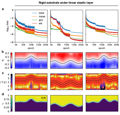
Fig. 5: Identification of substrate shape underneath a periodic linear elastic layer. a, The various loss components that enforce the solution to match the surface measurement data, satisfy the governing equations, and obey the eikonal regularization, are being minimized during the training process. b,c, The final level-set function $\phi$ and its gradient magnitude $|\nabla\phi|$ show the effect of the eikonal regularization, which makes $\phi$ a signed distance function in narrow band along the material boundary. d, The final material density $\rho$ reveals the shape of the buried rigid substrate.

Contrary to the matrix problem, this setup only provides access to measurements on the top surface, and the hidden geometry to be discovered is not completely surrounded by the elastic material. Our TO framework is nevertheless able to detect the correct depths and shapes of the hidden substrates (Fig. 5). This example demonstrates the versatility of the framework in adapting to various problem setups.

Discussion

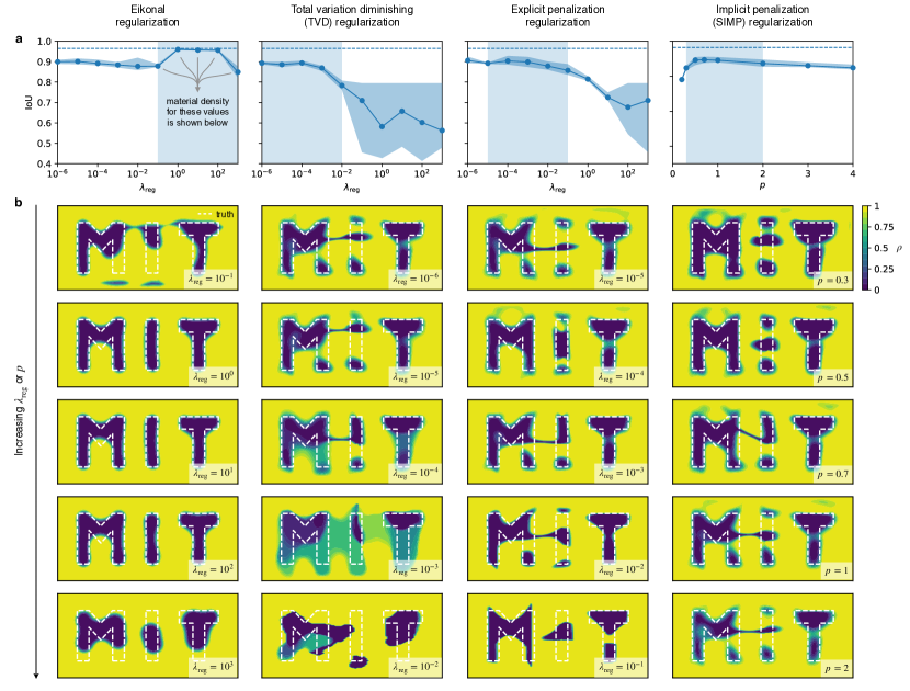
Fig. 6: Comparison between eikonal regularization and alternative regularizations. a, The eikonal regularization achieves a high IoU (intersection over union, a geometry detection accuracy metric equal to 1 in the perfect case) above 0.95 for any value of the regularization weight $\lambda_{\mathrm{reg}}$ within a range spanning three orders of magnitude. The results are consistent over 4 random initializations of the neural networks parameters, with the circles reporting the average value and the shade reporting the highest and lowest values. By contrast, the total variation diminishing (TVD), explicit penalization, and Solid Isotropic Material with Penalization (SIMP) regularizations never exceed IoU values above 0.93, with larger variability among realizations. b, The final material density $\rho$ obtained with each regularization mechanism for various values of the regularization weight $\lambda_{\mathrm{reg}}$ or exponent $p$ (shown in a by the shaded areas) demonstrates the efficacy of the eikonal regularization. The evolution of the solution during training using the eikonal regularization and $\lambda_{\mathrm{reg}}=1$ is shown in Supplementary Movie 2.

As with any TO method relying on a material density field to parameterize the geometry, the success of our PINN-based framework hinges on the presence of an appropriate regularization mechanism to penalize intermediate density values. Although we have shown that our novel eikonal regularization leads to consistently accurate results, other regularization approaches have been employed in classical adjoint-based TO methods [18, 51]. These include the total variation dimishing (TVD) regularization [10, 39] that penalizes the $L_{1}$ norm of the density gradient $\nabla\rho$, the explicit penalization regularization [3] that penalizes the integral over the domain of $\rho(1-\rho)$, and the Solid Isotropic Material with Penalization (SIMP) approach [7] that relates material properties such as the shear modulus and the material density through a power-law with exponent $p$. The latter is the most popular regularization mechanism in structural optimization [8]. However, when implemented in our PINN-based framework for the detection of hidden geometries, these methods yield inferior results to the eikonal regularization (Fig. 6). Indeed, we compare all four approaches on a challenging test case involving a linear elastic rectangular matrix pulled from the top and bottom and containing soft inclusions in the shape of the letters M, I, and T (case 19, Tab. 1). The measurements consist of the displacement along the outer boundary, similar to the previous square matrix examples. We consider different values of the regularization weight $\lambda_{\mathrm{reg}}$ (for the eikonal, TVD and explicit penalization regularizations) and the exponent $p$ (for the SIMP regularization), and solve the inverse problem using four random initializations of the neural networks in each case. Not only was the eikonal regularization the only one to find the right shapes, it did so over three orders of magnitude of $\lambda_{\mathrm{reg}}$, demonstrating a desirable robustness with respect to $\lambda_{\mathrm{reg}}$ (Fig. 6).

Thanks to the flexibility of the PINN framework, adapting our approach to various scenarios involving partial information, three-dimensional geometries, or other types of noninvasive imaging experiments (e.g. using thermal [6], acoustic [14], electric [12], or magnetic [37] loading) should be straightforward. As an illustration, we identify a hidden inclusion in a nonlinearly conducting matrix using partially unknown thermal loading (Supplementary Information), mimicking an inaccessible surface. This experiment reveals our method’s ability to generate good results without further modifications even when the forward problem is ill-posed, which would require including the unknown boundary condition as an additional optimization variable in a classical adjoint-based approach.

In conclusion, we have presented a PINN-based TO framework with a novel eikonal regularization, which we have applied to the noninvasive detection of hidden inclusions. By representing the geometry through a material density field combined with a novel eikonal regularization, our framework is able to discover the number, shapes and locations of hidden structures, without any prior knowledge required regarding the number or the types of shapes to expect. Finally, the idea of parameterizing geometries of arbitrary topologies with a material density field regularized with the eikonal constraint opens a pathway for PINNs to be applied to a wide range of design optimization problems constrained by physical governing equations. These include, for instance, the design of lenses that achieve targeted optical properties [41, 38] or the design of structures and metamaterials that exhibit desirable mechanical, acoustic, or thermal properties [8, 30, 32].

Methods

Governing equations

The two plane-strain elasticity inverse problems considered in this study (Fig. 1) are defined in a two-dimensional domain $\Omega\subset\mathbb{R}^{2}$ formed by the union of the elastic body $\mathcal{B}$ and the voids or inclusions. Denoting with $\mathbf{x}=(x_{1},x_{2})\in\Omega$ the planar spatial coordinates, the hidden geometrical layout of voids or inclusions is characterized by a material density $\rho(\mathbf{x})$ equal to 1 in the body $\mathcal{B}$ and 0 in the voids or inclusions.

Small-deformation linear elasticity

We first consider the case where the elastic body and inclusions consist of linear elastic materials, with Young’s modulus $E$ and Poisson’s ratio $\nu$ for the body, and Young’s modulus $\bar{E}$ and Poisson’s ratio $\bar{\nu}$ for the inclusions. Voids and rigid inclusions correspond to the limits $\bar{E}\rightarrow 0$ and $\bar{E}\rightarrow\infty$, respectively. The deformation of the elastic body containing the inclusions is described by a vector field $\boldsymbol{\psi}(\mathbf{x})=(\mathbf{u}(\mathbf{x}),\boldsymbol{\sigma}(\mathbf{x}))$, where $\mathbf{u}(\mathbf{x})$ is a planar displacement field with components $u_{i}(\mathbf{x})$ and $\boldsymbol{\sigma}(\mathbf{x})$ is a Cauchy stress tensor with components $\sigma_{ij}(\mathbf{x})$. Indices $i$ and $j$ will hereafter always range from 1 to 2.

The governing PDEs comprise the equilibrium equations

$$\sum_{j}\frac{\partial\sigma_{ij}}{\partial x_{j}}=0,\quad\mathbf{x}\in\Omega,$$ (7)

as well as a linear elastic constitutive law $F(\boldsymbol{\sigma},\nabla\mathbf{u},\rho)=0$ that we will express in two different but equivalent ways, depending on whether the inclusions are softer or stiffer than the matrix. For voids and soft inclusions, we consider the constitutive law in stress-strain form,

$$\boldsymbol{\sigma} =\rho\left[\lambda\,\mathrm{tr}(\boldsymbol{\epsilon})\,\mathbf{I}+2\mu\,\boldsymbol{\epsilon}\right],$$

$$\quad\ (1-\rho)\left[\bar{\lambda}\,\mathrm{tr}(\boldsymbol{\epsilon})\,\mathbf{I}+2\bar{\mu}\,\boldsymbol{\epsilon}\right],\quad\mathbf{x}\in\Omega,$$ (8)

where $\boldsymbol{\epsilon}=(\nabla\mathbf{u}+\nabla\mathbf{u}^{T})/2$ is the infinitesimal strain tensor, $\mathrm{tr}(\boldsymbol{\epsilon})$ denotes its trace, $\lambda=E\nu/(1+\nu)(1-2\nu)$ and $\mu=E/2(1+\nu)$ are the Lamé constants of the body, and $\bar{\lambda}=\bar{E}\bar{\nu}/(1+\bar{\nu})(1-2\bar{\nu})$ and $\bar{\mu}=\bar{E}/2(1+\bar{\nu})$ are the Lamé constants of the inclusions. Notice that the case of voids, the stress vanishes in the $\rho=0$ regions. For stiff and rigid inclusions, we consider the constitutive law in the inverted strain-stress form

$$\boldsymbol{\epsilon} =\rho\left[\frac{1+\nu}{E}\boldsymbol{\sigma}-\frac{\nu(1+\nu)}{E}\,\mathrm{tr}(\boldsymbol{\sigma})\,\mathbf{I}\right]$$

$$\quad\ (1-\rho)\left[\frac{1+\bar{\nu}}{\bar{E}}\boldsymbol{\sigma}-\frac{\bar{\nu}(1+\bar{\nu})}{\bar{E}}\,\mathrm{tr}(\boldsymbol{\sigma})\,\mathbf{I}\right],\quad\mathbf{x}\in\Omega,$$ (9)

where $\mathrm{tr}(\boldsymbol{\sigma})$ is the trace of the stress tensor. This relation differs from the three-dimensional one due to the plane strain assumption. Notice that the case of rigid inclusions, the strain vanishes in the $\rho=0$ regions.

The boundary conditions on $\partial\Omega$ and surface displacement measurement locations $\partial\Omega^{m}$ are different in the two problems. For the elastic matrix (Fig. 1a), the domain is $\Omega=[-0.5,0.5]\times[-0.5,0.5]$ and the boundary conditions are

$$\boldsymbol{\sigma}(\mathbf{x})\mathbf{n}(\mathbf{x}) =-P_{o}\mathbf{e}_{1}, \mathbf{x}\in\{-0.5,0.5\}\times[-0.5,0.5],$$ (10a)

$$\boldsymbol{\sigma}(\mathbf{x})\mathbf{n}(\mathbf{x}) =\mathbf{0},\quad \mathbf{x}\in[-0.5,0.5]\times\{-0.5,0.5\}.$$ (10b)

The measurement locations $\partial\Omega^{m}$ are distributed along the entire external boundary $\partial\Omega$. In the case of the M, I, T inclusions (case 19, Tab. 1), the boundary conditions (10) are changed to account for the fact that the matrix is pulled from the top and bottom boundaries and covers the domain $\Omega=[-1,1]\times[-0.5,0.5]$. For the elastic layer (Fig. 1b), the domain is $\Omega=[0,1]\times[-0.5,0]$ and the boundary conditions are

$$\boldsymbol{\sigma}(\mathbf{x})\mathbf{n}(\mathbf{x}) =-P_{o}\mathbf{e}_{2}, \mathbf{x}\in[0,1]\times\{0\},$$ (11a)

$$\mathbf{u} =\mathbf{0}, \mathbf{x}\in[0,1]\times\{-0.5\},$$ (11b)

as well as periodic for the displacement and traction on $\mathbf{x}\in\{0,1\}\times[-0.5,0]$. The measurement locations $\partial\Omega^{m}$ are distributed along the top surface $\partial\Omega_{t}=[0,1]\times\{0\}$.

The geometry identification problem that we solve can then be stated as follows. Given surface displacement measurements $\mathbf{u}_{i}^{m}$ at locations $\mathbf{x}_{i}\in\partial\Omega^{m}$, find the distribution of material density $\rho$ in $\Omega$ such that the difference between the predicted and measured surface displacements vanish, that is,

$$\mathbf{u}(\mathbf{x}_{i})=\mathbf{u}_{i}^{m},\quad\mathbf{x}_{i}\in\partial\Omega^{m}.$$ (12)

The predicted displacement field must satisfy the equilibrium equation (7), the constitutive relation (8) or (9), and the boundary conditions (10) or (11).

Large-deformation nonlinear hyperelasticity

Next, we consider the case where the elastic body consists of an incompressible Neo-Hookean hyperelastic material with shear modulus $\mu$. We now have to distinguish between the reference (undeformed) and current (deformed) configurations. We denote by $\mathbf{x}=(x_{1},x_{2})\in\Omega$ and $\mathbf{y}=(y_{1},y_{2})\in\Omega^{*}$ the coordinates in the reference and deformed configurations, respectively, with $\Omega^{*}$ the deformed image of $\Omega$. The displacement field $\mathbf{u}(\mathbf{x})$ with components $u_{i}(\mathbf{x})$ moves an initial position $\mathbf{x}\in\Omega$ into its current location $\mathbf{y}=\mathbf{x}+\mathbf{u}(\mathbf{x})\in\Omega^{*}$. In order to formulate the governing equations and boundary conditions in the reference configuration $\Omega$, we need to introduce the first Piola-Kirchhoff stress tensor $\mathbf{S}(\mathbf{x})$ with components $S_{ij}(\mathbf{x})$. Unlike the Cauchy stress tensor, the first Piola-Kirchhoff stress tensor is defined in $\Omega$ and is not symmetric. The deformation of the elastic body is then described by the vector field $\boldsymbol{\psi}(\mathbf{x})=(\mathbf{u}(\mathbf{x}),\mathbf{S}(\mathbf{x}),p(\mathbf{x}))$ defined over $\Omega$, where $p(\mathbf{x})$ is a pressure field that serves to enforce the incompressibility constraint.

The equilibrium equations are

$$\sum_{j}\frac{\partial S_{ij}}{\partial x_{j}}=0,\quad\mathbf{x}\in\Omega,$$ (13)

where the derivatives in $\nabla_{\mathbf{x}}$ are taken with respect to the reference coordinates $\mathbf{x}$. We only consider the presence of voids so that the nonlinear constitutive law $F(\mathbf{S},\nabla_{\mathbf{x}}\mathbf{u},p,\rho)=0$ is simply expressed as

$$\mathbf{S}=\rho\left[-p\mathbf{F}^{-T}+\mu\mathbf{F}\right],\quad\mathbf{x}\in\Omega,$$ (14)

where $\mathbf{F}(\mathbf{x})=\mathbf{I}+\nabla_{\mathbf{x}}\mathbf{u}(\mathbf{x})$ is the deformation gradient tensor. Notice that the stress vanishes in the $\rho=0$ regions. Finally, we have the incompressibility constraint

$$\rho\left[\det(\mathbf{F})-1\right]=0,\quad\mathbf{x}\in\Omega,$$ (15)

which turns itself off in the $\rho=0$ regions since voids do not deform in a way that preserves volume.

We only treat the matrix problem (Fig. 1a) in this hyperelastic case. The domain is $\Omega=[-0.5,0.5]\times[-0.5,0.5]$ and the boundary conditions are

$$\mathbf{S}(\mathbf{x})\mathbf{n}_{0}(\mathbf{x}) =-P_{o}\mathbf{e}_{1}, \mathbf{x}\in\{-0.5,0.5\}\times[-0.5,0.5],$$ (16a)

$$\mathbf{S}(\mathbf{x})\mathbf{n}_{0}(\mathbf{x}) =\mathbf{0},\quad \mathbf{x}\in[-0.5,0.5]\times\{-0.5,0.5\}.$$ (16b)

As in the linear elastic case, the measurement locations $\partial\Omega^{m}$ are distributed along the entire external boundary $\partial\Omega$.

The geometry identification problem can then be stated identically as in the linear elastic case. This time, the predicted displacement field must satisfy the equilibrium equation (13), the constitutive relation (14), the incompressibility condition (15), and the boundary conditions (16).

Rescaling

The various physical quantities involved in the elasticity inverse problem span a wide range of scales; for instance, displacements may be orders of magnitude smaller than the length scale associated with the geometry. Thus, we rescale all physical quantities into nondimensional values of order one, as also done in [29]. Lengths are rescaled with the width $L$ of the elastic matrix or elastic layer, tractions and stresses with the magnitude $P_{o}$ of the applied traction at the boundaries, and displacements with the ratio $LP_{o}/E$, where $E$ is the Young’s modulus of the elastic material (in the hyperelastic case, we use the equivalent Young’s modulus $E=3\mu$, where $\mu$ is the shear modulus of the hyperelastic material). This rescaling is critical to enable the neural networks underlying our framework to handle elasticity problems across a wide range of material moduli and applied loads.

Solution methodology

Here, we describe in detail the application of our TO framework to the solution of the two plane-strain elasticity inverse problems formulated in the introduction. We will treat separately the small-deformation linear elasticity case and the large-deformation hyperelasticity case.

Small-deformation linear elasticity

Since the problem is described by the physical quantities $\boldsymbol{\psi}=(u_{1},u_{2},\sigma_{11},\sigma_{22},\sigma_{12})$, we introduce the neural network approximations

$$u_{1}(\mathbf{x}) =\bar{u}_{1}(\mathbf{x};\boldsymbol{\theta}_{1}),$$ (17a)

$$u_{2}(\mathbf{x}) =\bar{u}_{2}(\mathbf{x};\boldsymbol{\theta}_{2}),$$ (17b)

$$\sigma_{11}(\mathbf{x}) =\bar{\sigma}_{11}(\mathbf{x};\boldsymbol{\theta}_{3}),$$ (17c)

$$\sigma_{22}(\mathbf{x}) =\bar{\sigma}_{22}(\mathbf{x};\boldsymbol{\theta}_{4}),$$ (17d)

$$\sigma_{12}(\mathbf{x}) =\bar{\sigma}_{12}(\mathbf{x};\boldsymbol{\theta}_{5}),$$ (17e)

$$\phi(\mathbf{x}) =\bar{\phi}(\mathbf{x};\boldsymbol{\theta}_{\phi}).$$ (17f)

The last equation represents the level-set neural network, which defines the material density as $\rho(\mathbf{x})=\bar{\rho}(\mathbf{x};\boldsymbol{\theta}_{\phi})=\mathrm{sigmoid}(\bar{\phi}(\mathbf{x};\boldsymbol{\theta}_{\phi})/\delta)$. We then formulate the loss function (3) by specializing the loss term expressions presented in results section to the linear elasticity problem. Omitting the $\boldsymbol{\theta}$’s for notational simplicity, we obtain

$$\mathcal{L}_{\mathrm{meas}}(\boldsymbol{\theta}_{\boldsymbol{\psi}}) =\frac{1}{|\partial\Omega^{m}|}\sum_{\mathbf{x}_{i}\in\partial\Omega^{m}}|\bar{\mathbf{u}}(\mathbf{x}_{i})-\mathbf{u}_{i}^{m}|^{2},$$ (18a)

$$\mathcal{L}_{\mathrm{gov}}(\boldsymbol{\theta}_{\boldsymbol{\psi}},\boldsymbol{\theta}_{\phi}) =\frac{1}{|\Omega^{d}|}\sum_{\mathbf{x}_{i}\in\Omega^{d}}|\mathbf{r}_{\mathrm{eq}}(\bar{\boldsymbol{\sigma}}(\mathbf{x}_{i}))|^{2}$$

$$\quad+\frac{1}{|\Omega^{d}|}\sum_{\mathbf{x}_{i}\in\Omega^{d}}|\mathbf{r}_{\mathrm{cr}}(\bar{\mathbf{u}}(\mathbf{x}_{i}),\bar{\boldsymbol{\sigma}}(\mathbf{x}_{i}),\bar{\rho}(\mathbf{x}_{i}))|^{2},$$ (18b)

$$\mathcal{L}_{\mathrm{eik}}(\boldsymbol{\theta}_{\phi}) =\frac{1}{|\Omega_{\mathrm{eik}}^{d}|}\sum_{\mathbf{x}_{i}\in\Omega_{\mathrm{eik}}^{d}}\left(|\nabla\bar{\phi}(\mathbf{x}_{i})|-1\right)^{2},$$ (18c)

where $\bar{\mathbf{u}}=(\bar{u}_{1},\bar{u}_{2})$ and $\bar{\boldsymbol{\sigma}}$ has components $\bar{\sigma}_{i,j}$, $i,j=1,2$. In (18b), the terms $\mathbf{r}_{\mathrm{eq}}$ and $\mathbf{r}_{\mathrm{cr}}$ refer to the residuals of the equilibrium equation (7) and the constitutive relation (8) or (9). The eikonal loss term is problem-independent and therefore identical to (6).

We note that instead of defining neural network approximations for the displacements and the stresses, we could define neural network approximations solely for the displacements, that is, $\boldsymbol{\psi}=(u_{1},u_{2})$. In this case, the loss term (18b) would only include the residual of the equilibrium equation (7), in which the stress components would be directly expressed in terms of the displacements and the material distribution using the constitutive relation (8). However, several recent studies [47, 25, 29, 48, 21, 26] have shown that the mixed formulation adopted in the present work results in superior accuracy and training performance, which could partly be explained by the fact that only first-order derivatives of the neural network outputs are involved since the displacements and stresses are only differentiated to first oder in (7) and (8). In our case, the mixed formulation holds the additional advantage that it enables us to treat stiff and rigid inclusions using the inverted constitutive relation (9) instead of (8). Finally, the mixed formulation allows us to directly integrate both displacement and traction boundary conditions into the output of the neural network approximations, as we describe in the next paragraph.

We design the architecture of the neural networks in such a way that they inherently satisfy the boundary conditions, treating the latter as hard constraints [17, 53]. For the elastic matrix, we do this through the transformations

$$\bar{u}_{1}(\mathbf{x};\boldsymbol{\theta}_{1}) =\bar{u}_{1}^{\prime}(\mathbf{x};\boldsymbol{\theta}_{1}),$$ (19a)

$$\bar{u}_{2}(\mathbf{x};\boldsymbol{\theta}_{2}) =\bar{u}_{2}^{\prime}(\mathbf{x};\boldsymbol{\theta}_{2}),$$ (19b)

$$\bar{\sigma}_{11}(\mathbf{x};\boldsymbol{\theta}_{3}) =(x-0.5)(x+0.5)\,\bar{\sigma}_{11}^{\prime}(\mathbf{x};\boldsymbol{\theta}_{3})+P_{o},$$ (19c)

$$\bar{\sigma}_{22}(\mathbf{x};\boldsymbol{\theta}_{4}) =(y-0.5)(y+0.5)\,\bar{\sigma}_{22}^{\prime}(\mathbf{x};\boldsymbol{\theta}_{4}),$$ (19d)

$$\bar{\sigma}_{12}(\mathbf{x};\boldsymbol{\theta}_{5}) =(x-0.5)(x+0.5)\cdot$$

$$\quad\ (y-0.5)(y+0.5)\,\bar{\sigma}_{12}^{\prime}(\mathbf{x};\boldsymbol{\theta}_{5}),$$ (19e)

$$\bar{\phi}(\mathbf{x};\boldsymbol{\theta}_{\phi}) =(x-0.5)(x+0.5)\cdot$$

$$\quad\ (y-0.5)(y+0.5)\,\bar{\phi}^{\prime}(\mathbf{x};\boldsymbol{\theta}_{\phi})+w,$$ (19f)

where the quantities with a prime denote the raw output of the neural network. In this way, the neural network approximations defined in (17) obey by construction the boundary conditions (10). Further, since we know that the elastic material is present all along the outer surface $\partial\Omega$, we define $\bar{\phi}$ so that $\phi=w$ on $\partial\Omega$, which ensures that $\rho=\mathrm{sigmoid}(\phi/\delta)\simeq 1$ on $\partial\Omega$ (recall that $w$ is such that $\mathrm{sigmoid}(w/2\delta)\simeq 1$). In the case of the M, I, T inclusions, these transformations are changed to reflect the fact that the matrix is wider and pulled from the top and bottom. For the periodic elastic layer, we introduce the transformations

$$\bar{u}_{1}(\mathbf{x};\boldsymbol{\theta}_{1}) =(y+0.5)\,\bar{u}_{1}^{\prime}(\cos x,\sin x,y;\boldsymbol{\theta}_{1}),$$ (20a)

$$\bar{u}_{2}(\mathbf{x};\boldsymbol{\theta}_{2}) =(y+0.5)\,\bar{u}_{2}^{\prime}(\cos x,\sin x,y;\boldsymbol{\theta}_{2}),$$ (20b)

$$\bar{\sigma}_{11}(\mathbf{x};\boldsymbol{\theta}_{3}) =\bar{\sigma}_{11}^{\prime}(\cos x,\sin x,y;\boldsymbol{\theta}_{3}),$$ (20c)

$$\bar{\sigma}_{22}(\mathbf{x};\boldsymbol{\theta}_{4}) =y\,\bar{\sigma}_{22}^{\prime}(\cos x,\sin x,y;\boldsymbol{\theta}_{4})-P_{o},$$ (20d)

$$\bar{\sigma}_{12}(\mathbf{x};\boldsymbol{\theta}_{5}) =y\,\bar{\sigma}_{12}^{\prime}(\cos x,\sin x,y;\boldsymbol{\theta}_{5}),$$ (20e)

$$\bar{\phi}(\mathbf{x};\boldsymbol{\theta}_{\phi}) =y(y+0.5)\,\bar{\phi}^{\prime}(\cos x,\sin x,y;\boldsymbol{\theta}_{\phi})$$

$$\quad+w(4y+1),$$ (20f)

so that the neural network approximations defined in (17) obey by construction the boundary conditions (11) and are periodic along the $x$ direction. Further, since we know that the elastic material is present all along the top surface $y=0$ and the rigid substrate is present all along the bottom surface $y=-0.5$, we define $\bar{\phi}$ so that $\phi=w$ for $y=0$ and $\phi=-w$ for $y=-0.5$, which ensures that $\rho=\mathrm{sigmoid}(\phi/\delta)\simeq 1$ for $y=0$ and $\rho\simeq 0$ for $y=-0.5$.

Large-deformation hyperelasticity

The problem is now described by the physical quantities $\boldsymbol{\psi}=(u_{1},u_{2},S_{11},S_{22},S_{12},S_{21},p)$. We therefore introduce the neural network approximations

$$u_{1}(\mathbf{x}) =\bar{u}_{1}(\mathbf{x};\boldsymbol{\theta}_{1}),$$ (21a)

$$u_{2}(\mathbf{x}) =\bar{u}_{2}(\mathbf{x};\boldsymbol{\theta}_{2}),$$ (21b)

$$S_{11}(\mathbf{x}) =\bar{S}_{11}(\mathbf{x};\boldsymbol{\theta}_{3}),$$ (21c)

$$S_{22}(\mathbf{x}) =\bar{S}_{22}(\mathbf{x};\boldsymbol{\theta}_{4}),$$ (21d)

$$S_{12}(\mathbf{x}) =\bar{S}_{12}(\mathbf{x};\boldsymbol{\theta}_{5}),$$ (21e)

$$S_{21}(\mathbf{x}) =\bar{S}_{21}(\mathbf{x};\boldsymbol{\theta}_{6}),$$ (21f)

$$p(\mathbf{x}) =\bar{p}(\mathbf{x};\boldsymbol{\theta}_{7}),$$ (21g)

$$\phi(\mathbf{x}) =\bar{\phi}(\mathbf{x};\boldsymbol{\theta}_{\phi}),$$ (21h)

and the material distribution is given by $\rho(\mathbf{x})=\bar{\rho}(\mathbf{x};\boldsymbol{\theta}_{\phi})=\mathrm{sigmoid}(\bar{\phi}(\mathbf{x};\boldsymbol{\theta}_{\phi})/\delta)$. We then formulate the loss function (3) by specializing the loss term expressions presented in Section General framework to the linear elasticity problem, using the governing equations given in Appendix Small-deformation linear elasticity. Omitting the $\boldsymbol{\theta}$’s for notational simplicity, we obtain

$$\mathcal{L}_{\mathrm{meas}}(\boldsymbol{\theta}_{\boldsymbol{\psi}}) =\frac{1}{|\partial\Omega^{m}|}\sum_{\mathbf{x}_{i}\in\partial\Omega^{m}}|\bar{\mathbf{u}}(\mathbf{x}_{i})-\mathbf{u}_{i}^{m}|^{2},$$ (22a)

$$\mathcal{L}_{\mathrm{gov}}(\boldsymbol{\theta}_{\boldsymbol{\psi}},\boldsymbol{\theta}_{\phi}) =\frac{1}{|\Omega^{d}|}\sum_{\mathbf{x}_{i}\in\Omega^{d}}|\mathbf{r}_{\mathrm{eq}}(\bar{\mathbf{S}}(\mathbf{x}_{i}))|^{2}$$

$$\quad+\frac{1}{|\Omega^{d}|}\sum_{\mathbf{x}_{i}\in\Omega^{d}}|\mathbf{r}_{\mathrm{cr}}(\bar{\mathbf{u}}(\mathbf{x}_{i}),\bar{\mathbf{S}}(\mathbf{x}_{i}),\bar{p}(\mathbf{x}_{i}),\bar{\rho}(\mathbf{x}_{i}))|^{2}$$

$$\quad+\frac{1}{|\Omega^{d}|}\sum_{\mathbf{x}_{i}\in\Omega^{d}}|\mathbf{r}_{\mathrm{inc}}(\bar{\mathbf{u}}(\mathbf{x}_{i}),\bar{\rho}(\mathbf{x}_{i}))|^{2},$$ (22b)

$$\mathcal{L}_{\mathrm{eik}}(\boldsymbol{\theta}_{\phi}) =\frac{1}{|\Omega_{\mathrm{eik}}^{d}|}\sum_{\mathbf{x}_{i}\in\Omega_{\mathrm{eik}}^{d}}\left(|\nabla\bar{\phi}(\mathbf{x}_{i})|-1\right)^{2},$$ (22c)

where $\bar{\mathbf{u}}=(\bar{u}_{1},\bar{u}_{2})$ and $\bar{\mathbf{S}}$ has components $\bar{S}_{i,j}$, $i,j=1,2$. In (22b), the terms $\mathbf{r}_{\mathrm{eq}}$, $\mathbf{r}_{\mathrm{cr}}$, and $\mathbf{r}_{\mathrm{inc}}$ refer to the residuals of the equilibrium equation (13), the constitutive relation (14), and the incompressibility constraint (15). The eikonal loss term is problem-independent and therefore identical to (6).

As in the linear elasticity case, we design the architecture of the neural networks in such a way that they inherently satisfy the boundary conditions. For the elastic matrix problem,

$$\bar{u}_{1}(\mathbf{x};\boldsymbol{\theta}_{1}) =\bar{u}_{1}^{\prime}(\mathbf{x};\boldsymbol{\theta}_{1}),$$ (23a)

$$\bar{u}_{2}(\mathbf{x};\boldsymbol{\theta}_{2}) =\bar{u}_{2}^{\prime}(\mathbf{x};\boldsymbol{\theta}_{2}),$$ (23b)

$$\bar{S}_{11}(\mathbf{x};\boldsymbol{\theta}_{3}) =(x-0.5)(x+0.5)\,\bar{S}_{11}^{\prime}(\mathbf{x};\boldsymbol{\theta}_{3})+P_{o},$$ (23c)

$$\bar{S}_{22}(\mathbf{x};\boldsymbol{\theta}_{4}) =(y-0.5)(y+0.5)\,\bar{S}_{22}^{\prime}(\mathbf{x};\boldsymbol{\theta}_{4}),$$ (23d)

$$\bar{S}_{12}(\mathbf{x};\boldsymbol{\theta}_{5}) =(y-0.5)(y+0.5)\,\bar{S}_{12}^{\prime}(\mathbf{x};\boldsymbol{\theta}_{5}),$$ (23e)

$$\bar{S}_{21}(\mathbf{x};\boldsymbol{\theta}_{6}) =(x-0.5)(x+0.5)\,\bar{S}_{21}^{\prime}(\mathbf{x};\boldsymbol{\theta}_{6}),$$ (23f)

$$\bar{p}(\mathbf{x};\boldsymbol{\theta}_{7}) =\bar{p}^{\prime}(\mathbf{x};\boldsymbol{\theta}_{7}),$$ (23g)

$$\bar{\phi}(\mathbf{x};\boldsymbol{\theta}_{\phi}) =(x-0.5)(x+0.5)\cdot$$

$$\quad\ (y-0.5)(y+0.5)\,\bar{\phi}^{\prime}(\mathbf{x};\boldsymbol{\theta}_{\phi})+w,$$ (23h)

where the quantities with a prime denote the raw output of the neural network. In this way, the neural network approximations defined in (21) obey by construction the boundary conditions of the problem. As before, since we know that the elastic material is present all along the outer surface $\partial\Omega$, we define $\bar{\phi}$ so that $\phi=w$ on $\partial\Omega$, which ensures that $\rho=\mathrm{sigmoid}(\phi/\delta)\simeq 1$ on $\partial\Omega$.

Architecture and training details

Here, we provide implementation details regarding the architecture of the deep neural networks, the training procedure and corresponding parameter values.

Neural network architecture

State variable fields of the form $\psi(\mathbf{x})$ are approximated using deep fully-connected neural networks that map the location $\mathbf{x}$ to the corresponding value of $\psi$ at that location. This map can be expressed as $\psi(\mathbf{x})=\bar{\psi}(\mathbf{x};\boldsymbol{\theta})$, and is defined by the sequence of operations

$$\mathbf{z}^{0} =\mathbf{x},$$ (24a)

$$\mathbf{z}^{k} =\sigma(\mathbf{W}^{k}\mathbf{z}^{k-1}+\mathbf{b}^{k}),\quad 1\leq k\leq\ell-1,$$ (24b)

$$\psi=\mathbf{z}^{\ell} =\mathbf{W}^{\ell}\mathbf{z}^{\ell-1}+\mathbf{b}^{\ell}.$$ (24c)

The input $\mathbf{x}$ is propagated through $\ell$ layers, all of which (except the last) take the form of a linear operation composed with a nonlinear transformation. Each layer outputs a vector $\mathbf{z}^{k}\in\mathbb{R}^{q_{k}}$, where $q_{k}$ is the number of ‘neurons’, and is defined by a weight matrix $\mathbf{W}^{k}\in\mathbb{R}^{q_{k}\times q_{k-1}}$, a bias vector $\mathbf{b}^{k}\in\mathbb{R}^{q_{k}}$, and a nonlinear activation function $\sigma(\cdot)$. Finally, the output of the last layer is assigned to $\psi$. The weight matrices and bias vectors, which parametrize the map from $\mathbf{x}$ to $\psi$, form a set of trainable parameters $\boldsymbol{\theta}=\{\mathbf{W}^{k},\mathbf{b}^{k}\}_{k=1}^{\ell}$.

The choice of the nonlinear activation function $\sigma(\cdot)$ and the initialization procedure for the trainable parameters $\boldsymbol{\theta}$ are both important factors in determining the performance of neural networks. While the tanh function has been a popular candidate in the context of PINNs [35], recent works by Refs. [52, 55] have shown that using sinusoidal activation functions can lead to improved training performance by promoting the emergence of small-scale features. In this work, we select the sinusoidal representation network (SIREN) architecture from Ref. [52], which combines the use of the sine as an activation function with a specific way to initialize the trainable parameters $\boldsymbol{\theta}$ that ensures that the distribution of the input to each sine activation function remains unchanged over successive layers. Specifically, each component of $\mathbf{W}^{k}$ is uniformly distributed between $-\sqrt{6/q_{k}}$ and $\sqrt{6/q_{k}}$ where $q_{k}$ is the number of neurons in layer $k$, and $\mathbf{b}^{k}=\mathbf{0}$, for $k=1,\dots,\ell$. Further, the first layer of the SIREN architecture is $\mathbf{z}^{1}=\sigma(\omega_{0}\mathbf{W}^{1}\mathbf{z}^{0}+\mathbf{b}^{1})$ instead of (24b), with the extra scalar $\omega_{0}$ promoting higher-frequency content in the output.

Training procedure

We construct the total loss function (3) and train the neural networks in TensorFlow 2. The training is performed using ADAM, a first-order gradient-descent-based algorithm with adaptive step size [31]. In each case, we repeat the training over four random initializations of the neural networks parameters and report the best results. Three tricks resulted in noticeably improved training performance and consistency:

• First, we found that pretraining the level-set neural network $\phi(\mathbf{x})=\bar{\phi}(\mathbf{x};\boldsymbol{\theta}_{\phi})$ in a standard supervised setting leads to much more consistent results over different initializations of the neural networks. During this pretraining step, carried out before the main optimization step in which all neural networks are trained to minimize the loss (3), we minimize the mean-square error

  $$\mathcal{L}_{\mathrm{sup}}(\boldsymbol{\theta}_{\phi})=\frac{1}{|\Omega^{d}|}\sum_{\mathbf{x}_{i}\in\Omega^{d}}|\bar{\phi}(\mathbf{x}_{i};\boldsymbol{\theta}_{\phi})-\phi_{i}|,$$ (25)

  where $\Omega^{d}$ is the same set of collocation points as in (5), the supervised labels $\phi_{i}=|\mathbf{x}_{i}|-0.25$ for the elastic matrix, and $\phi_{i}=y_{i}+0.25$ for the elastic layer. The material density $\bar{\rho}(\mathbf{x};\boldsymbol{\theta}_{\phi})=\mathrm{sigmoid}(\bar{\phi}(\mathbf{x};\boldsymbol{\theta}_{\phi})/\delta)$ obtained at the end of this pretraining step is one outside a circle of radius 0.25 centered at the origin for the elastic matrix, and it is one above the horizontal line $y=-0.25$ for the elastic layer. This choice for the supervised labels is justified by the fact that $\rho$ is known to be one along the outer boundary of the domain $\Omega$ for the elastic matrix, and it is known to be one (zero) along the top (bottom) boundary of $\Omega$ for the elastic layer.

• Second, during the main optimization in which all neural networks are trained to minimize the loss (3), we evaluate the loss component $\mathcal{L}_{\mathrm{gov}}$ in (5) using a different subset, or mini-batch, of residual points from $\Omega^{d}$ at every iteration. Such a mini-batching approach has been reported to improve the convergence of the PINN training process [54, 15], corroborating our own observations. In our case, we choose to divide the set $\Omega^{d}$ into 10 different mini-batches of size $|\Omega^{d}|/10$, which are then employed sequentially to evaluate $\mathcal{L}_{\mathrm{gov}}$ during each subsequent gradient update

  $$\boldsymbol{\theta}_{\boldsymbol{\psi}}^{k+1} =\boldsymbol{\theta}_{\boldsymbol{\psi}}^{k}-\alpha_{\boldsymbol{\psi}}(k)\nabla_{\boldsymbol{\theta}_{\boldsymbol{\psi}}}\mathcal{L}(\boldsymbol{\theta}_{\boldsymbol{\psi}}^{k},\boldsymbol{\theta}_{\phi}^{k}),$$ (26a)

  $$\boldsymbol{\theta}_{\phi}^{k+1} =\boldsymbol{\theta}_{\phi}^{k}-\alpha_{\phi}(k)\nabla_{\boldsymbol{\theta}_{\phi}}\mathcal{L}(\boldsymbol{\theta}_{\boldsymbol{\psi}}^{k},\boldsymbol{\theta}_{\phi}^{k}).$$ (26b)

  An epoch of training, which is defined as one complete pass through the whole set $\Omega^{d}$, therefore consists of 10 gradient updates.

• Third, the initial nominal step size $\alpha_{\boldsymbol{\psi}}$ governing the learning rate of the physical quantities neural networks is set to be 10 times larger than its counterpart $\alpha_{\phi}$ governing the learning rate of the level-set neural network. This results in a separation of time scales between the rate of change of the physical quantities neural networks and that of the level-set neural network, which is motivated by the idea that physical quantities should be given time to adapt to a given geometry before the geometry itself changes.

Parameter values

The parameter values described below apply to all results presented in this paper.

• Neural network architecture. For all cases except the M, I, T inclusions (case 19, Tab. 1), we opted for neural networks with 4 hidden layers of 50 neurons each, which we found to be a good compromise between expressivity and training time. For the M, I, T inclusions, we used 6 hidden layers with 100 neurons each. Further, we choose $\omega_{0}=10$ as the scalar appearing in the first layer of the SIREN architecture.

• Collocation and measurements points. In the square and rectangle elastic matrix problems, we consider that the boundary displacement is measured along each of the four external boundaries at 100 equally-spaced points, which amounts to $|\partial\Omega^{m}|=400$. In the elastic layer problem, we consider that the boundary displacement is measured along the top boundary at 100 equally-spaced points, which amounts to $|\partial\Omega^{m}|=100$. For both geometries except the M, I, T inclusions, the set of collocation points $\Omega^{d}$ consists of 10000 points distributed in $\Omega$ with a Latin Hypercube Sampling (LHS) strategy, yielding 10 mini-batches containing 1000 points each. For the M, I, T inclusions, $\Omega^{d}$ consists of 50000 points, yielding 50 mini-batches containing 1000 points each.

• Training parameters. The pretraining of the level-set neural network is carried out using the ADAM optimizer with nominal step size $10^{-3}$ over 800 training epochs, employing the whole set $\Omega^{d}$ to compute the gradient of $\mathcal{L}_{\mathrm{sup}}$ at each update step. The main optimization, during which all neural networks are trained to minimize the total loss (3), is carried out using the ADAM optimizer. For the matrix cases except the M, I, T inclusions, we use a total of 150k training epochs starting from a nominal step size $10^{-4}$ for the level-set neural network and $10^{-3}$ for the other neural networks. This step size is reduced to $10^{-4}$ for all neural networks at 60k epochs, and again to $10^{-5}$ at 120k epochs. The schedule is the same for the elastic layer cases, with the difference that we use a total of 200k training epochs. For the matrix case with the M, I, T inclusions, we use a total of 50k epochs (note that each epoch contains 5 times as many mini-batches as in the other cases) starting from a nominal step size $10^{-4}$ for the level-set neural network and $10^{-3}$ for the other neural networks. This step size is reduced to $10^{-4}$ for all neural networks at 16k epochs, and again to $10^{-5}$ at 40k epochs. Finally, the scalar weights in the loss (3) are assigned the values $\lambda_{\mathrm{meas}}=10$, $\lambda_{\mathrm{gov}}=1$, and $\lambda_{\mathrm{reg}}=1$ for all cases. We also multiply the second term of $\mathcal{L}_{\mathrm{gov}}$ in (18b) and (22b) with a scalar weight $\lambda_{\mathrm{cr}}=10$.

FEM simulations

The FEM simulations that provide the boundary displacement data and the ground truth are performed in the software Abaqus, using its Standard (implicit) solver. The list of all cases considered in provided in Tab. 1 for the elastic matrix setup (Fig. 1a) and in Tab. 2 for the periodic elastic layer setup (Fig. 1b). Every case is meshed using a linear density of 200 elements per unit length along each boundary, corresponding to between 25k to 80k total elements depending on domain size as well as number and shapes of voids or inclusions. We employ bilinear quadrilateral CPE4 plain-strain elements for the cases involving a linear elastic material, and their hybrid constant-pressure counterpart CPE4H for the cases involving a hyperelastic material. We apply a load $P_{o}/E=0.01$ for the cases involving a linear elastic material, and a load $P_{o}/E=0.173$ for the cases involving a hyperelastic material.

Case	Geometry	Matrix	Inclusion
1	Two circles	LE	V
2		HE	V
3	One star and one rectangle	LE	V
4		LE	LE-soft
5		LE	LE-stiff
6		LE	R
7		HE	V
8	One slit	LE	V
9		HE	V
10	One U	LE	V
11		LE	LE-soft
12		LE	LE-stiff
13		LE	R
14		HE	V
15	One T	LE	V
16		HE	V
17	Four circles	LE	V
18		HE	V
19	One M, one I and one T	LE	LE-soft

Tab. 1: List of all elastic matrix (Fig. 1a) cases, classified according to the geometry of the inclusions and the elastic properties of the matrix and inclusions. LE: linear elastic with $E=1$ and $\nu=0.3$; HE: incompressible Neo-Hookoean hyperelastic with $\mu=0.38$; LE-soft: linear elastic with $E=0.2$, $\nu=0.3$; LE-stiff: linear elastic with $E=5$, $\nu=0.3$; R: rigid; V: void.

Case	Geometry	Layer	Substrate
20	Sinusoidal	LE	R
21	Pulse	LE	R
22	Random wave	LE	R

Tab. 2: List of all periodic elastic layer (Fig. 1b) cases, classified according to the shape of the substrate. LE: linear elastic with $E=1$ and $\nu=0.3$; R: rigid.

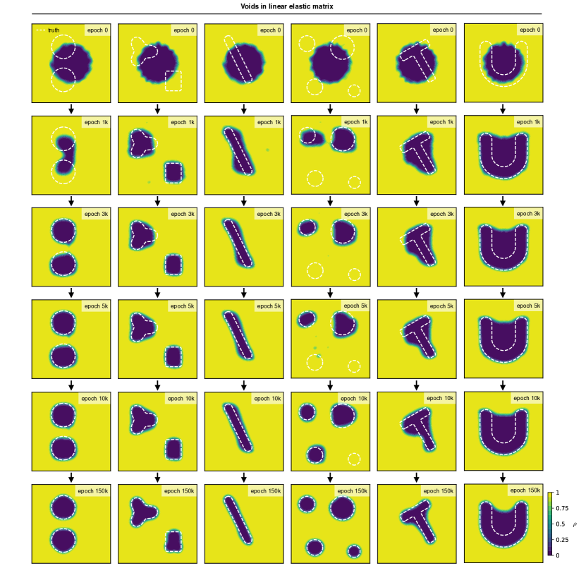
Extended Data Fig. 1: Identification of voids in a linear elastic matrix. Evolution of the material density during the training process for the cases reported in Fig. 4a-d.

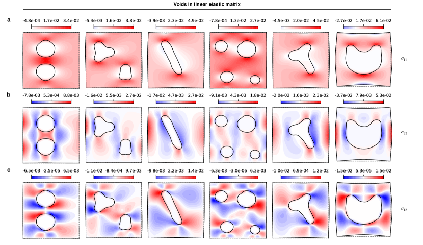
Extended Data Fig. 2: Identification of voids in a linear elastic matrix. Final Cauchy stress components $\sigma_{xx}$ (a), $\sigma_{yy}$ (b), and $\sigma_{xy}$ (c), displayed in the deformed configuration obtained from the final displacement components $u_{1}$ and $u_{2}$, for the cases reported in Fig. 4a-d. The grey dotted lines show the outline of the matrix surface in the reference configuration.

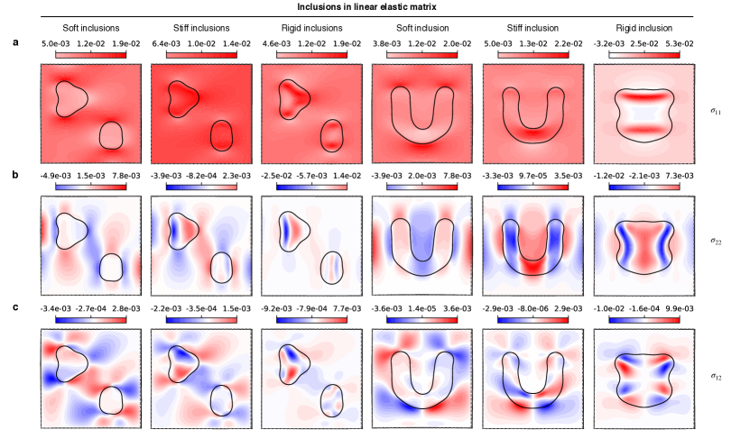
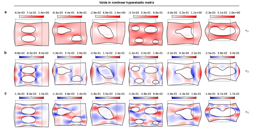
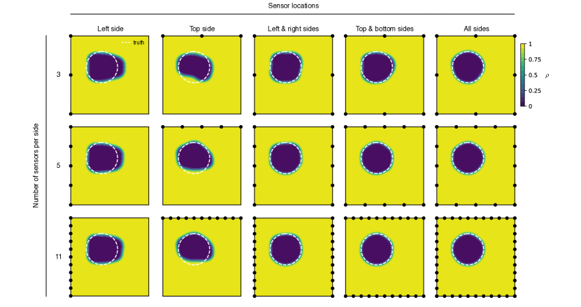
Extended Data Fig. 3: Identification of inclusions in a linear elastic matrix. Final Cauchy stress components $\sigma_{xx}$ (a), $\sigma_{yy}$ (b), and $\sigma_{xy}$ (c), displayed in the deformed configuration obtained from the final displacement components $u_{1}$ and $u_{2}$, for the cases reported in Fig. 4e. The grey dotted lines show the outline of the matrix surface in the reference configuration.

Extended Data Fig. 4: Identification of voids in a nonlinear hyperelastic matrix. Final Cauchy stress components $\sigma_{xx}$ (a), $\sigma_{yy}$ (b), and $\sigma_{xy}$ (c), displayed in the deformed configuration obtained from the final displacement components $u_{1}$ and $u_{2}$, for the cases reported in Fig. 4f. The grey dotted lines show the outline of the matrix surface in the reference configuration.

Extended Data Fig. 5: Effect of sparse measurements on the identification of voids in a linear elastic matrix with one circle-shaped void. Final material density obtained in our framework when using fewer measurement locations and restricting the number of measurements to a subset of the outer surfaces.

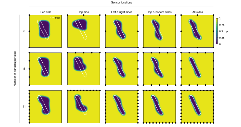
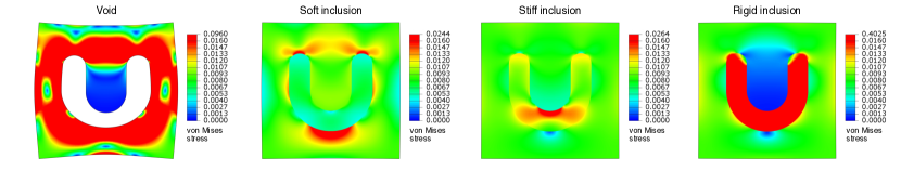
Extended Data Fig. 6: Effect of sparse measurements on the identification of voids in a linear elastic matrix with one star-shaped and one rectangle-shaped void. Final material density obtained in our framework when using fewer measurement locations and restricting the number of measurements to a subset of the outer surfaces.

Extended Data Fig. 7: Effect of sparse measurements on the identification of voids in a linear elastic matrix with one slit-shaped void. Final material density obtained in our framework when using fewer measurement locations and restricting the number of measurements to a subset of the outer surfaces.

Extended Data Fig. 8: Stress distribution in a linear elastic matrix for different types of U-shaped inclusions. The von Mises stress obtained in Abaqus for U-shaped inclusions with different constitutive properties reveals that the concave part of the matrix is subject to very little stress in the case of a void or rigid inclusion. Note also that stiff and rigid inclusions ‘strengthen’ the matrix, as opposed to the void and soft inclusion that ‘soften’ the matrix.

References

- Adalsteinsson and Sethian [1995] D. Adalsteinsson and J. A. Sethian. A fast level set method for propagating interfaces. Journal of computational physics, 118(2):269–277, 1995.
- Adler and Holder [2021] A. Adler and D. Holder. Electrical impedance tomography: methods, history and applications. CRC Press, 2021.
- Allaire and Kohn [1993] G. Allaire and R. Kohn. Topology optimization and optimal shape design using homogenization. In Topology design of structures, pages 207–218. Springer, 1993.
- Allaire et al. [2004] G. Allaire, F. Jouve, and A.-M. Toader. Structural optimization using sensitivity analysis and a level-set method. Journal of computational physics, 194(1):363–393, 2004.
- Ameur et al. [2004] H. B. Ameur, M. Burger, and B. Hackl. Level set methods for geometric inverse problems in linear elasticity. Inverse Problems, 20(3):673, 2004.
- Banks et al. [1990] H. T. Banks, F. Kojima, and W. P. Winfree. Boundary estimation problems arising in thermal tomography. Inverse problems, 6(6):897, 1990.
- Bendsøe [1989] M. P. Bendsøe. Optimal shape design as a material distribution problem. Structural optimization, 1(4):193–202, 1989.
- Bendsoe and Sigmund [2003] M. P. Bendsoe and O. Sigmund. Topology optimization: theory, methods, and applications. Springer Science & Business Media, 2003.
- Bonnet and Constantinescu [2005] M. Bonnet and A. Constantinescu. Inverse problems in elasticity. Inverse problems, 21(2):R1, 2005.
- Chan and Tai [2004] T. F. Chan and X.-C. Tai. Level set and total variation regularization for elliptic inverse problems with discontinuous coefficients. Journal of Computational Physics, 193(1):40–66, 2004.
- Chen and Dal Negro [2022] Y. Chen and L. Dal Negro. Physics-informed neural networks for imaging and parameter retrieval of photonic nanostructures from near-field data. APL Photonics, 7(1):010802, 2022.
- Cheney et al. [1999] M. Cheney, D. Isaacson, and J. C. Newell. Electrical impedance tomography. SIAM review, 41(1):85–101, 1999.
- Cherepenin et al. [2001] V. Cherepenin, A. Karpov, A. Korjenevsky, V. Kornienko, A. Mazaletskaya, D. Mazourov, and D. Meister. A 3d electrical impedance tomography (eit) system for breast cancer detection. Physiological measurement, 22(1):9, 2001.
- Colton et al. [2000] D. Colton, J. Coyle, and P. Monk. Recent developments in inverse acoustic scattering theory. Siam Review, 42(3):369–414, 2000.
- Daw et al. [2022] A. Daw, J. Bu, S. Wang, P. Perdikaris, and A. Karpatne. Rethinking the importance of sampling in physics-informed neural networks. arXiv preprint arXiv:2207.02338, 2022.
- Dissanayake and Phan-Thien [1994] M. Dissanayake and N. Phan-Thien. Neural-network-based approximations for solving partial differential equations. Communications in Numerical Methods in Engineering, 10(3):195–201, 1994.
- Dong and Ni [2021] S. Dong and N. Ni. A method for representing periodic functions and enforcing exactly periodic boundary conditions with deep neural networks. Journal of Computational Physics, 435:110242, 2021.
- Dorn and Lesselier [2006] O. Dorn and D. Lesselier. Level set methods for inverse scattering. Inverse Problems, 22(4):R67, 2006.
- Dorn et al. [2000] O. Dorn, E. L. Miller, and C. M. Rappaport. A shape reconstruction method for electromagnetic tomography using adjoint fields and level sets. Inverse problems, 16(5):1119, 2000.
- Eschenauer et al. [1994] H. A. Eschenauer, V. V. Kobelev, and A. Schumacher. Bubble method for topology and shape optimization of structures. Structural optimization, 8(1):42–51, 1994.
- Gladstone et al. [2022] R. J. Gladstone, M. A. Nabian, and H. Meidani. Fo-pinns: A first-order formulation for physics informed neural networks. arXiv preprint arXiv:2210.14320, 2022.
- Griffiths [2001] H. Griffiths. Magnetic induction tomography. Measurement science and technology, 12(8):1126, 2001.
- Gropp et al. [2020] A. Gropp, L. Yariv, N. Haim, M. Atzmon, and Y. Lipman. Implicit geometric regularization for learning shapes. In International Conference on Machine Learning, pages 3789–3799. PMLR, 2020.
- Guo et al. [2014] X. Guo, W. Zhang, and W. Zhong. Doing topology optimization explicitly and geometrically?a new moving morphable components based framework. Journal of Applied Mechanics, 81(8), 2014.
- Haghighat et al. [2021] E. Haghighat, M. Raissi, A. Moure, H. Gomez, and R. Juanes. A physics-informed deep learning framework for inversion and surrogate modeling in solid mechanics. Computer Methods in Applied Mechanics and Engineering, 379:113741, 2021.
- Harandi et al. [2023] A. Harandi, A. Moeineddin, M. Kaliske, S. Reese, and S. Rezaei. Mixed formulation of physics-informed neural networks for thermo-mechanically coupled systems and heterogeneous domains. arXiv preprint arXiv:2302.04954, 2023.
- Haslinger and Mäkinen [2003] J. Haslinger and R. A. Mäkinen. Introduction to shape optimization: theory, approximation, and computation. SIAM, 2003.
- Hellier [2013] C. J. Hellier. Handbook of nondestructive evaluation. McGraw-Hill Education, 2013.
- Henkes et al. [2022] A. Henkes, H. Wessels, and R. Mahnken. Physics informed neural networks for continuum micromechanics. Computer Methods in Applied Mechanics and Engineering, 393:114790, 2022.
- Kadic et al. [2019] M. Kadic, G. W. Milton, M. van Hecke, and M. Wegener. 3d metamaterials. Nature Reviews Physics, 1(3):198–210, 2019.
- Kingma and Ba [2014] D. P. Kingma and J. Ba. Adam: A method for stochastic optimization. arXiv preprint arXiv:1412.6980, 2014.
- Kollmann et al. [2020] H. T. Kollmann, D. W. Abueidda, S. Koric, E. Guleryuz, and N. A. Sobh. Deep learning for topology optimization of 2d metamaterials. Materials & Design, 196:109098, 2020.
- Lagaris et al. [1998] I. E. Lagaris, A. Likas, and D. I. Fotiadis. Artificial neural networks for solving ordinary and partial differential equations. IEEE transactions on neural networks, 9(5):987–1000, 1998.
- Lee et al. [2000] H. S. Lee, C. J. Park, and H. W. Park. Identification of geometric shapes and material properties of inclusions in two-dimensional finite bodies by boundary parameterization. Computer Methods in Applied Mechanics and Engineering, 181(1-3):1–20, 2000.
- Lu et al. [2021a] L. Lu, X. Meng, Z. Mao, and G. E. Karniadakis. Deepxde: A deep learning library for solving differential equations. SIAM Review, 63(1):208–228, 2021a.
- Lu et al. [2021b] L. Lu, R. Pestourie, W. Yao, Z. Wang, F. Verdugo, and S. G. Johnson. Physics-informed neural networks with hard constraints for inverse design. SIAM Journal on Scientific Computing, 43(6):B1105–B1132, 2021b.
- Ma and Soleimani [2017] L. Ma and M. Soleimani. Magnetic induction tomography methods and applications: A review. Measurement Science and Technology, 28(7):072001, 2017.
- Ma et al. [2021] W. Ma, Z. Liu, Z. A. Kudyshev, A. Boltasseva, W. Cai, and Y. Liu. Deep learning for the design of photonic structures. Nature Photonics, 15(2):77–90, 2021.
- Mei et al. [2016] Y. Mei, R. Fulmer, V. Raja, S. Wang, and S. Goenezen. Estimating the non-homogeneous elastic modulus distribution from surface deformations. International Journal of Solids and Structures, 83:73–80, 2016.
- Mei et al. [2021] Y. Mei, Z. Du, D. Zhao, W. Zhang, C. Liu, and X. Guo. Moving morphable inclusion approach: an explicit framework to solve inverse problem in elasticity. Journal of Applied Mechanics, 88(4), 2021.
- Molesky et al. [2018] S. Molesky, Z. Lin, A. Y. Piggott, W. Jin, J. Vucković, and A. W. Rodriguez. Inverse design in nanophotonics. Nature Photonics, 12(11):659–670, 2018.
- Mowlavi and Nabi [2023] S. Mowlavi and S. Nabi. Optimal control of PDEs using physics-informed neural networks. Journal of Computational Physics, 473:111731, 2023.
- Osher and Fedkiw [2003] S. Osher and R. Fedkiw. Level set methods and dynamic implicit surfaces. Springer-Verlag, 2003.
- Osher and Sethian [1988] S. Osher and J. A. Sethian. Fronts propagating with curvature-dependent speed: Algorithms based on hamilton-jacobi formulations. Journal of computational physics, 79(1):12–49, 1988.
- Raissi et al. [2019] M. Raissi, P. Perdikaris, and G. E. Karniadakis. Physics-informed neural networks: A deep learning framework for solving forward and inverse problems involving nonlinear partial differential equations. Journal of Computational physics, 378:686–707, 2019.
- Raissi et al. [2020] M. Raissi, A. Yazdani, and G. E. Karniadakis. Hidden fluid mechanics: Learning velocity and pressure fields from flow visualizations. Science, 367(6481):1026–1030, 2020.
- Rao et al. [2021] C. Rao, H. Sun, and Y. Liu. Physics-informed deep learning for computational elastodynamics without labeled data. Journal of Engineering Mechanics, 147(8):04021043, 2021.
- Rezaei et al. [2022] S. Rezaei, A. Harandi, A. Moeineddin, B.-X. Xu, and S. Reese. A mixed formulation for physics-informed neural networks as a potential solver for engineering problems in heterogeneous domains: comparison with finite element method. Computer Methods in Applied Mechanics and Engineering, 401:115616, 2022.
- Robledo et al. [2009] L. Robledo, M. Carrasco, and D. Mery. A survey of land mine detection technology. International Journal of Remote Sensing, 30(9):2399–2410, 2009.
- Sahli Costabal et al. [2020] F. Sahli Costabal, Y. Yang, P. Perdikaris, D. E. Hurtado, and E. Kuhl. Physics-informed neural networks for cardiac activation mapping. Frontiers in Physics, 8:42, 2020.
- Sigmund and Maute [2013] O. Sigmund and K. Maute. Topology optimization approaches. Structural and Multidisciplinary Optimization, 48(6):1031–1055, 2013.
- Sitzmann et al. [2020] V. Sitzmann, J. Martel, A. Bergman, D. Lindell, and G. Wetzstein. Implicit neural representations with periodic activation functions. Advances in Neural Information Processing Systems, 33:7462–7473, 2020.
- Sukumar and Srivastava [2022] N. Sukumar and A. Srivastava. Exact imposition of boundary conditions with distance functions in physics-informed deep neural networks. Computer Methods in Applied Mechanics and Engineering, 389:114333, 2022.
- Wight and Zhao [2021] C. L. Wight and J. Zhao. Solving Allen-Cahn and Cahn-Hilliard equations using the adaptive physics informed neural networks. Communications in Computational Physics, 29(3):930–954, 2021.
- Wong et al. [2021] J. C. Wong, C. Ooi, A. Gupta, and Y.-S. Ong. Learning in sinusoidal spaces with physics-informed neural networks. arXiv preprint arXiv:2109.09338, 2021.
- Zhang et al. [2022] E. Zhang, M. Dao, G. E. Karniadakis, and S. Suresh. Analyses of internal structures and defects in materials using physics-informed neural networks. Science advances, 8(7):eabk0644, 2022.