Finding Minimum-Cost Explanations for Predictions made by Tree Ensembles

Abstract

The ability to explain why a machine learning model arrives at a particular prediction is crucial when used as decision support by human operators of critical systems. The provided explanations must be provably correct, and preferably without redundant information, called minimal explanations. In this paper, we aim at finding explanations for predictions made by tree ensembles that are not only minimal, but also minimum with respect to a cost function. To this end, we first present a highly efficient oracle that can determine the correctness of explanations, surpassing the runtime performance of current state-of-the-art alternatives by several orders of magnitude when computing minimal explanations. Secondly, we adapt an algorithm called MARCO from related works (calling it m-MARCO) for the purpose of computing a single minimum explanation per prediction, and demonstrate an overall speedup factor of two compared to the MARCO algorithm which enumerates all minimal explanations. Finally, we study the obtained explanations from a range of use cases, leading to further insights of their characteristics. In particular, we observe that in several cases, there are more than 100,000 minimal explanations to choose from for a single prediction. In these cases, we see that only a small portion of the minimal explanations are also minimum, and that the minimum explanations are significantly less verbose, hence motivating the aim of this work.

1 Introduction

In many practical applications of machine learning, the ability to explain why a prediction model arrives at a certain decision is crucial (?). Although significant progress has been made to understand the intricacies of machine learning systems and how their predictions can be explained (for a comprehensive survey, see e.g., ?, ?), there are still open research questions. In this work, we are concerned with the use of machine learning models in critical decision support systems such as medical diagnosis and flight management systems, where a human acts in a loop, working together with the system to make critical decisions. In such cases, explanations for predictions may enable their system operators to make informed interventions of autonomous actions when explanations appear unjustified. More specifically, we aim at providing explanations that are provably correct and without redundant information for predictions made by a class of machine learning models called tree ensembles.

To illustrate the notion and usefulness of such explanations, consider a fictive bank-loan application support system, realized by the simple decision tree depicted by Figure 1.

Figure 1: A fictive bank-loan application processing system, where a positive outcome indicates that the applicant should be denied a loan.

Suppose the system processes a particular applicant with a low income, low education, no criminal records, and a couple of missed payments, and the system denies the applicant a bank-loan. When explaining to the applicant why the requested loan is denied, information about criminal records may be omitted since that particular feature does not contribute to the outcome of the prediction. Furthermore, if the applicant requests a new assessment after getting a salary raise (so that the applicant no longer has a low income), the system would respond the same. Consequently, an explanation only needs to include information about two of the four features; low education and missed payments. We say that explanations that are correct and without redundant information are minimal. Typically, there are several minimal explanations to choose from, potentially hundreds of thousands for large systems. By associating each minimal explanation with a cost computed by a domain-specific cost function, we can order them to find one that is most desirable for the problem at hand, called a minimum explanation. To this end, this paper contributes with the following.

• We formalize a sound and complete oracle for determining the correctness of an explanation in the abstract interpretation framework, designed specifically for tree ensembles.

• We demonstrate the performance of our oracle in a case study from related work that computes minimal explanations, and conclude an overall speedup factor of 2,400 compared to current state-of-the-art.

• We demonstrate that, in the presence of a highly efficient oracle, it is possible to enumerate all minimal explanations for several predictions made by non-trivial tree ensembles.

• We propose an algorithm m-MARCO which is an adaptation of the MARCO algorithm from related work (?) for the purpose of computing an explanation that is minimum, and demonstrate an overall speedup factor of two compared to the MARCO algorithm which enumerates all minimal explanations.

• We demonstrate that m-MARCO is significantly faster than a branch and bound approach used in some SMT solvers to compute counter-examples of unsatisfiable formulas.

We also provide an implementation of our algorithms, together with logs and automated scripts to reproduce our results.

The rest of this paper is structured as follows. Section 2 provides preliminaries on the computation of minimal and minimum explanations, the MARCO algorithm, decision trees and tree ensembles, and abstract interpretation. In Section 3, we relate our contributions to earlier works. In Section 4, we formalize an oracle in the abstract interpretation framework that can determine the correctness of explanations, and in Section 5 algorithms for computing minimal and minimum explanations. In Section 6, we study the runtime performance of the formalized algorithms, and investigate characteristics of the explanations computed in that study, e.g.,. how many minimal and minimum explanations there are for a given prediction. Finally, Section 7 concludes the paper. There is also an Appendix A with a supplementary algorithm for reasoning about tree ensembles trained on multi-class classification problems, and more detailed results from the runtime performance study.

2 Preliminaries

In this section, we bring together notions from several fields in order to establish a common vocabulary for the rest of the paper. First, we define the notion of valid explanations with respect to a particular prediction, and how we can distinguish between them based on their verbosity. We then review the MARCO algorithm presented elsewhere, which can be used in conjunction with an oracle to enumerate all minimal explanations for a particular prediction. Next, we formalize the function making predictions in this paper; the prediction function for tree ensembles trained on classification problems. Finally, we communicate basic ideas that are essential for sound reasoning with abstract interpretation, concepts that are foundational when constructing an oracle we later use to compute desirable explanations.

2.1 Notation

We use lower-cased letters to denote functions and scalars, and upper-cased letters to denote sets. The number of input dimensions of functions are typically denoted $n$, and the number of output dimensions $m$. Input variables are normally named $x$, and output variables $y$. A function named $f$ that accepts an argument $x$ and is parameterized with a model $M$ is denoted $f(x;M)$. Tuples of scalars are annotated with a bar, e.g., $\bar{x}=(x_{1},\ldots,x_{n})$, while variables and functions associated with abstract interpretation are annotated with a hat, e.g., $\widehat{x}$. Finally, we denote the power set over a set $S$ as $\raisebox{1.79993pt}{\Large$\wp$}(S)$.

2.2 Minimizing the Verbosity of Explanations

The idea of using formal methods to minimize the verbosity of explanations we explore in this paper originates from the problem of simplifying Boolean functions into prime implicants (?), with later extensions to first-order logic for the purpose of abductive reasoning (?). More recently, these ideas have been applied to the explanation of predictions made by different types of machine learning models (e.g., ?, ?, ?, ?, ?). These related works are discussed further in Section 3. We now start by defining the notion of a valid explanation.

Definition 1 (Valid Explanation).

Let $f:\mathcal{D}^{n}\rightarrow\mathcal{D}$ be a function, $(x_{1},\ldots,x_{n})$ variables ranging over elements in $\mathcal{D}$, and $(c_{1},\ldots,c_{n})\in\mathcal{D}^{n}$ constants. An explanation $E\subseteq\{(x_{1},c_{1}),\ldots,(x_{n},c_{n})\}$ is valid with respect to a prediction $f(c_{1},\ldots,c_{n})\mapsto d$ iff

$$\Big{(}\bigwedge_{(x_{i},c_{i})\in E}x_{i}=c_{i}\Big{)}\to f(x_{1},\ldots,x_{n})=d.$$

For example, consider the binary classifier $f(x_{1},x_{2},x_{3})=(x_{1}\leq 0\land x_{2}\leq 0)\lor x_{3}\leq 0$, and the prediction $p:f(0,0,0)\mapsto True$. Clearly, there are several valid explanations for $p$, e.g., $E_{1}=\{(x_{1},0),(x_{2},0),(x_{3},0)\}$, $E_{2}=\{(x_{1},0),(x_{2},0)\}$, and $E_{3}=\{(x_{3},0)\}$, some of which capture redundant information with respect to their validity as explanations for $p$, and thus may be minimized. In order to distinguish between several valid explanations, we define the concept of a minimal explanation.

Definition 2 (Minimal Explanation).

An explanation $E$ that is valid with respect to a prediction $f(c_{1},\ldots,c_{n})\mapsto d$ is minimal iff removing elements from $E$ invalidates the explanation, i.e.,

$$\forall A\subset E,\Big{(}\bigwedge_{(x_{i},c_{i})\in A}x_{i}=c_{i}\Big{)}\not\to f(x_{1},\ldots,x_{n})=d.$$

When formalized in propositional logic, minimal explanations are closely related to prime implicants, and thus are sometimes called PI-explanations (e.g., ?). Other works sometimes call them subset-minimal explanations (e.g., ?), or sufficient reasons (e.g., ?).

In general, there may be several minimal explanations for a particular prediction. Depending on the application domain and target audience, different explanations may be preferable (?). In the medical domain for example, some explanations may require that the target audience has medical training in order to comprehend concepts captured by variables associated with an explanation, while other explanations may be more suitable for patients, albeit more verbose. In this work, we capture this need by providing the means to choose different cost functions depending on the target audience.

Definition 3 (Minimum Explanation).

A minimal explanation $E$ is minimum with respect to a cost function $g:\raisebox{1.79993pt}{\Large$\wp$}(\{1,\ldots,n\})\rightarrow\mathbb{R}$ iff indices in $E$ minimize $g$, i.e.,

$$\{i:(x_{i},c_{i})\in E\}\in\operatorname*{arg\,min}_{\raisebox{1.79993pt}{\Large$\wp$}(\{1,\ldots,n\})}(g).$$

Note that there may be several minimum explanations for a particular prediction. We call the special case $E=\emptyset$ the empty explanation, which is only valid for predictions made by a constant function. Some works call minimum explanations minimal-cost explanations (e.g., ?), and when formalized in a satisfiability modulo theory, they are closely related to minimum satisfying assignments. In this work, we focus on explanations that are minimum with respect to the weighted sum $g(I;W)=\sum_{i\in I}w_{i}$, where $W=(w_{1},\ldots,w_{n})\in\mathbb{R}_{\geq 0}^{n}$ is an $n$-tuple with positive weights. Due to lack of domain knowledge in many datasets used by researchers for experimental studies, however, all weights in our experiments are fixed to one. This is equivalent to the cost function $g(I)=|I|$, which is sometimes called cardinality-minimal explanations (e.g., ?).

2.3 Exploring the Power Set Lattice of a Constraint System

In many areas of computer science, we are confronted with unsatisfiable constraint systems that need to be decomposed for pin-pointing causes of their unsatisfiability. These decompositions may be represented by elements in a power set lattice $(\raisebox{1.79993pt}{\Large$\wp$}(C),\subseteq)$, where $C$ is the set of constraints put on the system, with $C=\emptyset$ representing the unconstrained system. Typically, we aim at finding elements adjacent to the frontier between satisfiable and unsatisfiable subsets of $C$, where the ones on the upper side (relative to the frontier) are called minimal unsatisfiable subsets (MUSes), and the lower ones are called maximal satisfiable subsets (MSSes).

Definition 4 (Minimal Unsatisfiable Subset).

A minimal unsatisfiable subset (MUS) of a set of constraints $C$ is a subset $S\subseteq C$ such that $S$ is unsatisfiable, and all proper subsets of $S$ are satisfiable.

Definition 5 (Maximal Satisfiable Subset).

A maximal satisfiable subset (MSS) of a set of constraints $C$ is a subset $S\subseteq C$ such that $S$ is satisfiable, and all proper supersets of $S$ are unsatisfiable.

In the context of linear programming, a MUS is often called an irreducible infeasible subsystem (IIS), and a MSS is often called a maximal feasible subset (MFS).

With access to an oracle that can determine satisfiability of subsets of a given constraint system, we can use a standard technique from linear programming called deletion filter (?) to shrink unsatisfiable subsets into MUSes, and similarly for growing satisfiable subsets into MSSes, as formalized in Algorithm 1 and 2, respectively.

1:function Shrink($S$)

2:     for each $i\in S$ do

3:         if not Oracle($S\backslash\{i\}$) then

4:              $S$ $\leftarrow$ $S\backslash\{i\}$

5:         end if

6:     end for

7:     return $S$

8:end function

Algorithm 1 Shrink an usatisfiable $S\subseteq C$ to a minimal unsatisfiable subset (MUS).

1:function Grow($S$)

2:     for each $i\in C\backslash S$ do

3:         if Oracle($S\cup\{i\}$) then

4:              $S$ $\leftarrow$ $S\cup\{i\}$

5:         end if

6:     end for

7:     return $S$

8:end function

Algorithm 2 Grow a satisfiable $S\subseteq C$ to a maximal satisfiable subset (MSS).

By encoding each element $i\in C$ as the absence of the $i$-th variable in an explanation (and thus the top element in the power set lattice encodes an empty explanation), we can derive a minimal explanation from the complement of a MSS, corresponding to a minimal correction set.

Definition 6 (Minimal Correction Set).

A minimal correction set (MCS) for a set of constraints $C$ is a subset $S\subseteq C$ such that $C\backslash S$ is a MSS.

To determine the satisfiability of elements from a lattice with such an encoding, in this paper we will use a valid explanation oracle.

Definition 7 (Valid Explanation Oracle).

Let $f:\mathcal{D}^{n}\rightarrow\mathcal{D}$ be a function, $(x_{1},\ldots,x_{n})$ variables ranging over elements in $\mathcal{D}$, $(c_{1},\ldots,c_{n})\in\mathcal{D}^{n}$ constants used in a prediction $p:f(c_{1},\ldots,c_{n})\mapsto d$, and $S\subseteq\{1,\ldots,n\}$ a set with elements that encode the absence of variables (with given indices) in an explanation. A valid explanation oracle is then defined as a procedure that decides the satisfaction of

$$\Big{(}\bigwedge_{i\in\{1,\ldots,n\}\backslash S}x_{i}=c_{i}\Big{)}\to f(x_{1},\ldots,x_{n})=d.$$

Some other works (?, ?) use a slightly different constraint system encoding to minimize explanations. In particular, some works encode elements in $C$ as the presence of variables in an explanation, rather than their absence as we do in this work. With that alternative encoding, one would use a negated valid explanation oracle to find a MUS, which would then contain indices of variables in a minimal explanation. We find our choice of encoding more natural for the problem of reducing the verbosity of explanations, but the alternatives are equivalent with respect to correctness.

2.3.1 Finding a Minimum Explanation

To find a minimum explanation, the power set lattice can be explored in order to determine the satisfiability of its elements in the following matter. Whenever a MSS is encountered, its corresponding MCS is computed, which captures all variable indices present in a minimal explanation, i.e., $E=\{(x_{i},c_{i}):i\in S\}$, where $S$ is a MCS. When all MCSes have been considered, the minimum explanations with respect to a cost function can be identified.

For example, let us again consider the classifier $f(x_{1},x_{2},x_{3})=(x_{1}\leq 0\land x_{2}\leq 0)\lor x_{3}\leq 0$ and the prediction $p:f(0,0,0)\mapsto True$ from Section 2.2. To find a minimum explanation for $p$, we first define the set of constraints $C=\{1,2,3\}$, where each element $i\in C$ encodes the constraint $x_{i}\leq 0$. We then construct the power set lattice $(\raisebox{1.79993pt}{\Large$\wp$}(C),\subseteq)$, and assess satisfiabillity of its members by querying a valid explanation oracle. Figure 2.3.1 illustrates a Hasse diagram of the constructed lattice, where each crossed over member encodes a set of absent variables which would yield non-valid explanations, and each bold one is a MSS. As can be seen in that figure, the lattice contains two MSSes; $\{1,2\}$ and $\{3\}$, which correspond to the two MCSes $\{3\}$ and $\{1,2\}$, respectively. Consequently, the prediction $p$ has two minimal explanations; $\{(x_{3},0)\}$ and $\{(x_{1},0),(x_{2},0)\}$. With the cost function $g(I)=|I|$, $\{(x_{3},0)\}$ is the only minimum explanation.

A Hasse diagram illustrating the power set lattice of a triple of constraints, where crossed over elements are unsatisfiable subsets, and bold elements are maximal satisfiable subsets.

2.3.2 The MARCO Algorithm

MARCO (short for Mapping Regions of Constraints) is an algorithm that identifies the frontier between satisfiable and unsatisfiable subsets of constraints. It was originally presented in two independent publications (?, ?), and later unified by the same set of authors (?). The algorithm depends on a seed generator that yields unexplored elements from $\raisebox{1.79993pt}{\Large$\wp$}(C)$, and maintains a state of explored elements with a set $M$. Normally, the number of elements in $M$ grows too large to reside in memory explicitly, hence one typically encodes them in an auxiliary formula as blocking constraints, which is solved using an off-the-shelf solver to extract new seeds. In this work, we leverage a standard seed generator realized using propositional logic, where previously explored elements are blocked with clauses in a Boolean CNF formula, and a SAT solver is used to generate new ones, as formalized in Algorithm 3.

Algorithm 3 When equipped with a SAT solver and an oracle, the MARCO algorithm can enumerate all MUSes and MSSes of a set of constraints.

1:$M$ $\leftarrow$ $\emptyset$ $\triangleright$ Initialize an empty Boolean CNF formula

2:while SAT($M$) do $\triangleright$ Repeatedly explore elements in the power set lattice

3:     $S$ $\leftarrow$ Solution($M$) $\triangleright$ Draw a seed from the lattice

4:     if Oracle($S$) then $\triangleright$ Check with oracle

5:         $S$ $\leftarrow$ Grow($S$) $\triangleright$ Seed is satisfiable, grow to a MSS

6:         $M$ $\leftarrow$ $M\cup\Big{\{}\bigwedge_{i\in C\backslash S}\phi_{i}$ } $\triangleright$ Block subsets of the obtained MSS

7:     else$\triangleright$ Seed is unsatisfiable

8:         $S$ $\leftarrow$ Shrink($S$) $\triangleright$ Shrink seed to a MUS

9:         $M$ $\leftarrow$ $M\cup\Big{\{}\bigwedge_{i\in S}\neg\phi_{i}$ } $\triangleright$ Block supersets of the obtained MUS

10:     end if

11:end while

The algorithm starts by defining a CNF formula $M$, initialized with an empty set of clauses (line 1). It then repeatedly checks the satisfiability of $M$ using a SAT solver (line 2). If $M$ is satisfiable, a solution $S$ is extracted from the solver, which is the new seed. The oracle is then queried for the satisfiability of $S$ (line 3). If the new seed is satisfiable, one climbs up in the lattice until a MSS is found (line 5). All subsets of the MSS are then blocked by appending a blocking clause to $M$ (line 6, where $\phi_{i}$ is a variable in the CNF formula). Otherwise, a MUS is found by climbing down the lattice, and all of its supersets are blocked (lines 8–9). This procedure is repeated until the SAT solver concludes that $M$ is unsatisfiable, in which case all MUSes and MSSes have been enumerated.

2.4 Decision Trees and Tree Ensembles

In machine learning, decision trees are used as predictive models to capture statistical properties of a system of interest. As the name suggests, the prediction function of a decision tree is parameterized by a tree structure, as exemplified by Figure 2. The tree is evaluated in a top-down manner, where decision rules associated with intermediate nodes determine which path to take towards the leaves, and ultimately which value to output.

Figure 2: A decision tree (to the left) partition an input space into disjoint regions (to the right), and associates each region with an output value.

In general, decision rules in decision trees may be non-linear and multivariate. Although researchers have demonstrated that decision trees with non-linear (?) and multivariate (?) decision rules can be useful, state-of-the-art implementations of tree-based machine learning models normally only contain univariate and linear decision rules, e.g., the popular machine learning libraries scikit-learn (?), XGBoost (?), and CatBoost (?). In this paper, we formalize the prediction function without explicitly stating decision rules.

Definition 8 (Decision Tree Prediction Function).

Let $X_{1},\ldots,X_{k}$ be a partition of an $n$-dimensional input space, $\bar{y_{1}},\ldots,\bar{y_{k}}$ values from an $m$-dimensional output space, and $T=\{(X_{1},\bar{y_{1}}),\ldots,(X_{k},\bar{y_{k}})\}$. The prediction function for a decision tree may then be defined as

$$t(\bar{x};T)=\begin{cases}\bar{y_{1}}&\text{if }\bar{x}\in X_{1},\\ &\vdots\\ \bar{y_{k}}&\text{if }\bar{x}\in X_{k}.\\ \end{cases}$$

When decision trees only contain univariate and linear decision rules, the partitioned input space $X_{1},\ldots,X_{k}$ forms adjacent hyperrectangles (boxes), as exemplified by Figure 2. A decision tree trained on a dataset with $n$ features may contain unreferenced variables, i.e., the tree only considers a subset of its input variables during prediction. This is typically the case in high-dimensional applications, or when the training dataset contains statistically insignificant features. Since such input variables never affect predictions, they never appear in minimal explanations. Consequently, we define the notion of variables referenced by a tree, which we later use in Section 5 to improve the runtime performance when computing minimal and minimum explanations.

Definition 9 (Variables Referenced by a Tree).

The variables referenced by a tree during predictions is a set of indices $V_{t}\subseteq\{1,\ldots,n\}$, defined as the union of all the dimensions its decision rules operate in.

For example, the decision tree illustrated in Figure 2 operates on $x_{1}$ and $x_{2}$, in which case $V_{t}=\{1,2\}$.

2.4.1 Tree Ensembles

Decision trees are known to suffer from overfitting, i.e., the model becomes too specialized towards training data, and the prediction function generalizes poorly when confronted with previously unseen inputs. To counteract overfitting of decision trees, several types of tree ensembles have been proposed, e.g., random forests (?) and gradient boosting machines (?). The different types of tree ensembles are normally distinguished by their learning algorithms, while their prediction functions have similar structure.

Definition 10 (Tree Ensemble Prediction Function).

Let $F=(T_{1},\ldots,T_{b})$ be a tuple of $b\in\mathbb{Z}_{+}$ decision trees (as defined by Definition 8), all sharing the same $n$-dimentional input space and $m$-dimentional output space. The prediction function for a tree ensemble may then be defined as

$$f(\bar{x};F)=\sum_{T\in F}t(\bar{x};T).$$

When leaves in decision trees are associated with tuples of scalars, $f$ applies the addition operator element-wise. Similar to a decision tree, an ensemble of trees may also only consider a subset of its input variables during prediction.

Definition 11 (Variables Referenced by a Tree Ensemble).

The variables referenced by a tree ensemble during predictions is a set of indices $V_{f}\subseteq\{1,\ldots,n\}$, defined as the union of all variables referenced by the individual trees in the ensemble.

2.4.2 Classification with Tree Ensembles

By training tree ensembles to predict probabilities, they can be used as classifiers. Classifiers trained using XGBoost have tree leaves that are associated with scalar values that are summed together in the logarithmic scale, followed by a transformation to the domain of probabilities. For binary classifications, the used transform function is the sigmoid function.

Definition 12 (Sigmoid Function).

The sigmoid function $p_{\sigma}$ is a function that transforms a real-valued input $z$ into an output value in the range $[0,1]$, and is defined as

$$p_{\sigma}(z)=\frac{1}{1+e^{-z}}.$$

With the sigmoid function defined, we can define the tree-based binary classifier.

Definition 13 (Tree-based Binary Classifier).

Let $F$ be a tree ensemble trained to predict the probability that a given input tuple $\bar{x}$ maps to one of two classes. A binary classifier $f_{bin}$ that discriminates between the two classes may then be defined as

$$f_{bin}(\bar{x};F)=p_{\sigma}\big{(}f(\bar{x};F)\big{)}>0.5.$$

To capture statistical properties of multi-class systems involving three or more classes, some machine learning libraries associate tree leaves with tuples of probabilities (e.g., ?), while others use the one-vs-rest classification paradigm (e.g., ?). Both of these approaches use the softmax function to transform values from the logarithmic domain to the domain of probabilities.

Definition 14 (Softmax Function).

The softmax function $p_{s}$ is a monotonic function that transforms a tuple of real-valued inputs into an output tuple with elements in the range $[0,1]$ such that those elements sum up to one, and is defined as

$$p_{s}(z_{1},\ldots,z_{m})=\frac{(e^{z_{1}},\ldots,e^{z_{m}})}{\sum\limits_{i=1}^{m}z_{i}}.$$

This work focuses on classifiers trained using XGBoost, which implements the one-vs-rest paradigm for multi-class classification.

Definition 15 (Tree-based Multi-class Classifier).

Let $C=(F_{1},\ldots,F_{m}$) be a collection of tree ensembles such that the $i$-th tree ensemble $F_{i}$ is trained to predict the probability that a given instance belongs to the $i$-th class. A multi-class classifier $f_{cls}$ that discriminates between the multiple classes may then be defined as

$$f_{cls}(\bar{x};C)=\min\Big{(}\operatorname*{arg\,max}_{\{1,\ldots,m\}}\Big{(}p_{s}\big{(}f(\bar{x};F_{1}),\ldots,f(\bar{x};F_{m})\big{)}\Big{)}\Big{)}$$

In principle, a multi-class classifier may predict that a given input belongs to different classes with the exact same probability, and thus may cause the argmax function to yield a set containing several classes. In these types of situations, machine learning libraries typically return only the class with the smallest index, being indifferent to the selected choice of class.

2.5 Abstract Interpretation of Computer Programs

Abstract interpretation is a framework introduced to facilitate sound and efficient reasoning about programs being analyzed by a compiler (?). The idea is to transform the source code of a program that computes values in a concrete domain into functions that operate in one or more abstract domains in which some analyses of interest are faster than in the corresponding concrete domain, but potentially less precise. For example, to initiate the analysis of a program running with floating-point numbers to work within the domain of intervals, an abstraction function $\alpha:\raisebox{1.79993pt}{\Large$\wp$}(\mathcal{FP})\rightarrow\mathcal{I}$ is used to map a set of values from the floating-point domain $\mathcal{FP}$ to values from the interval domain $\mathcal{I}$. Analogously, a concretization function $\gamma:\mathcal{I}\rightarrow\raisebox{1.79993pt}{\Large$\wp$}(\mathcal{FP})$ is used to map an interval to a set of floating-point numbers. Abstraction and concretization mappings that operate on certain domains lead to a property called Galois connection that ensures sound reasoning with abstract interpretation (?).

Definition 16 (Galois Connection).

Let $\alpha:\mathcal{D}\rightarrow\mathcal{A}$ and $\gamma:\mathcal{A}\rightarrow\raisebox{1.79993pt}{\Large$\wp$}(\mathcal{D})$ be two monotone functions. A Galois connection $\raisebox{1.79993pt}{\Large$\wp$}(\mathcal{D})\galois{\alpha}{\gamma}\mathcal{A}$ exist between the concrete domain $\mathcal{D}$ and the abstract domain $\mathcal{A}$ iff

$$\forall X\in\raisebox{1.79993pt}{\Large$\wp$}(\mathcal{D}),X\subseteq\gamma(\alpha(X)),$$

$$\forall\widehat{x}\in\mathcal{A},\widehat{x}=\alpha(\gamma(\widehat{x})).$$

To perform the analysis, the program is interpreted in the abstract domain by evaluating sequences of abstract values, operators, and transformers.

Definition 17 (Abstract Transformer).

An abstract transformer $\widehat{f}:\mathcal{A}\rightarrow\mathcal{A}$ is an abstract counterpart of a concrete function $f:\mathcal{D}\rightarrow\mathcal{D}$, but one that operates in the abstract domain.

When using abstract interpretation in a reasoning context, soundness can be ensured by proving that there exists a Galois connection between the concrete and abstract domains, hence all computations performed in the abstract domain with the corresponding transformers are conservative.

Definition 18 (Conservative Transformer).

Let $\alpha:\raisebox{1.79993pt}{\Large$\wp$}(\mathcal{D})\rightarrow\mathcal{A}$ be an abstraction function, and $\gamma:\mathcal{A}\rightarrow\raisebox{1.79993pt}{\Large$\wp$}(\mathcal{D})$ a concretization function. An abstract transformer $\widehat{f}:\mathcal{A}\rightarrow\mathcal{A}$ is conservative with respect to a concrete function $f:\mathcal{D}\rightarrow\mathcal{D}$ iff

$$\forall X\in\raisebox{1.79993pt}{\Large$\wp$}(\mathcal{D}),\forall x\in X,f(x)\in\gamma(\widehat{f}(\alpha(X))).$$

Abstract transformers for standard operators in concrete domains or sets over such domains, e.g., addition and inclusion, can analogously be defined in a conservative manner. In this paper, we leverage an abstract interpreter that performs computations in the interval domain.

Definition 19 (Interval Domain).

The interval domain $\mathcal{I}$ contains abstract values $\widehat{x}$ that capture sets of values from a concrete domain $\mathcal{D}$ using a range defined by a lower and upper inclusive bound, i.e., $\widehat{x}=[l,u]$, where $l,u\in\mathcal{D},l\leq u$ are the lower and upper bound, respectively. Table 1 defines natural abstraction and concretization functions, operators, and constants associated with the interval domain.

Name	Definition
Abstraction	$\alpha(V)=[\min V,\max V]$
Concretization	$\gamma([v_{1},v_{2}])=\{v:v_{1}\leq v\leq v_{2}\}$
Top	$\top=\alpha(\mathcal{D})$
Bottom	$\bot=\alpha(\emptyset)$
Addition	$\widehat{v}+\widehat{u}=[v_{1}+u_{1},v_{2}+u_{2}]$
Join	$\widehat{v}\sqcup\widehat{u}=[\min(v_{1},u_{1}),\max(v_{2},u_{2})]$
Meet	$\widehat{v}\sqcap\widehat{u}=\begin{cases}\bot\text{ if }\max(v_{1},u_{1})>\min(v_{2},u_{2}),\\ [\max(v_{1},u_{1}),\min(v_{2},u_{2})]\text{ otherwise}\\ \end{cases}$
Greater than	$\widehat{v}>\widehat{u}=\begin{cases}[0,0]\text{ if }\min(u_{1},u_{2})>\max(v_{1},v_{2}),\\ [1,1]\text{ if }\min(v_{1},v_{2})>\max(u_{1},u_{2}),\\ [0,1]\text{ otherwise}\\ \end{cases}$

Table 1: Abstract interpretation in the interval domain $\mathcal{I}$ over values from the concrete domain $\mathcal{D}$, where $V\subseteq\mathcal{D}$, $v,v_{1},v_{2},u_{1},u_{2}\in\mathcal{D}$, and $\widehat{v}=[v_{1},v_{2}],\widehat{u}=[u_{1},u_{2}]\in\mathcal{I}$.

Abstract interpretation of programs with multiple variables in the interval domain form hyperrectangles, in which case the domain is often referred to as the Box domain.

3 Related Works

The use of formal methods to prove correctness of explanations for predictions made by machine learning systems has been promoted fairly recently. ? (?) compute minimal explanations for classifications made by Bayesian networks. By compiling the prediction function of Bayesian networks into an ordered (non-binary) decision diagram, they are able to compute explanations efficiently. The computational challenges instead lie in the compilation of Bayesian networks into decision diagrams, rather than the computation of explanations (?). ? (?) demonstrate that off-the-shelf constraint solvers, e.g., SMT and MILP solvers, can be used to minimize explanations if the prediction function can be represented within the used reasoning engine. They assess scalability in terms of time taken to compute explanations for predictions made by several neural networks trained on different datasets. Through experiments, they demonstrate that a state-of-the-art MILP solver typically outperforms most SMT solvers, and that computing explanations for models trained on high-dimensional inputs is significantly more demanding than low-dimensional problems. Compared to that work, we develop a framework to embed a reasoning engine that is tailored specifically for tree ensembles to achieve improved runtime performance. ? (?) also compute explanations for neural networks, but use reasoning engines designed specifically for the analysis of neural networks. They compare two different algorithms for computing a minimum explanation, both based on prior work, but with several novel algorithmic improvements. One algorithm is based on a branch-and-bound approach (?), and the other is based on hitting sets (?). In their Appendix, they demonstrate that their improved branch-and-bound approach is typically faster than the hitting sets approach. In this work, we use a similar branch-and-bound approach to compute minimum explanations, but for predictions made by tree ensembles, a model which has demonstrated greater predictive capabilities than neural networks in several practical applications (?). ? (?) use a SAT solver to compute minimal explanations for non-trivial random forests (100 trees with depths ranging from three to eight). They also show that this computational problem is DP-complete, i.e., the class of computations involving both NP-complete and coNP-complete sub-problems. Around the same time, ? (?) also used a SAT solver to compute minimal explanations for random forests, but with a different encoding. They argue for the use of random forests as surrogates for models for which no direct SAT-encoding exists. ? (?) present the notion of majority reasons for the purpose of explaining predictions made by random forests. These explanations are significantly less computationally demanding to compute than minimal explanations, at the potential expense of some verbosity. They also show that the problem of computing a minimum explanation is $\Sigma_{2}^{p}$-complete, i.e., NP-complete with a coNP oracle. In this work, we aim at reducing the runtime needed to compute explanations, but without compromising on verbosity. ? (?) propose an approach that uses a MaxSAT-based oracle when computing minimal explanations of predictions made by tree ensembles. The approach is based on the application of the deletion filter (?), which is evaluated on gradient boosting machines trained on 21 different datasets. They formulate the hard part of the MaxSAT encoding as a CNF formula, where intervals are represented by auxiliary Boolean variables, while the validity of an explanation is encoded as weighted soft clauses that can be optimized to find a minimal explanation. In this work, we also use a deletion filter, but with an oracle based on abstract interpretation which is designed specifically for tree ensembles. Compared to the MaxSAT approach, our oracle operates on an implicit DNF encoding of relaxed constraints that captures input-output relations derived from a tree ensemble. The relaxed constraints are captured by abstract values from the interval domain, which are enumerated and iteratively tightened in an abstraction-refinement loop (?). Furthermore, we tackle the computation of minimum explanations, and complete enumeration of all minimal explanations. The MARCO algorithm (?) has been applied to a broad range of problems, including for enumerating minimal explanations of prediction made by decision lists (?) and monotonic classifiers (?). Compared to those works, we demonstrate that the pairing of the MARCO algorithm with an oracle formalized in the abstract interpretation framework can make the enumeration of all minimal explanations for several predictions made by non-trivial tree ensembles tractable. We also adapt MARCO for computing explanations that are minimum with respect to the weighted sum $g(I;W)=\sum_{i\in I}w_{i}$, where $I\subseteq\{1,\ldots,n\}$ and $W=(w_{1},\ldots,w_{n})\in\mathbb{R}_{\geq 0}^{n}$, demonstrating a speedup factor of two compared to the enumeration of all minimal explanations. A very recent work (?) tackles the problem of removing redundancy in explanations for predictions made by decision trees. Our work applies to ensembles of decision trees, and aims at computing explanations that are minimum with respect to a domain-specific cost function, motivated by the comprehensive field guide on explainability by ? (?).

4 Constructing an Oracle based on Abstract Interpretation

In this section, we formalize the inner workings of a valid explanation oracle (see Definition 7), designed specifically for tree ensembles using the concept of abstract interpretation. First, we define abstract transformers, which are necessary building blocks when constructing the oracle (Section 4.1). Next, we define the abstract valid explanation oracle, together with an abstraction-refinement approach which ensures that abstractions that are too conservative are refined into more precise ones (Section 4.2). Finally, we assemble the building blocks into a sound and complete valid explanation oracle (Section 4.3). Since the input dimension of a tree ensemble is typically different from its output dimension, we sometimes subscript abstraction and concretization functions to indicate which dimensionality they operate on, e.g., $\raisebox{1.79993pt}{\Large$\wp$}(\mathcal{D}^{n})\galois{\alpha_{n}}{\gamma_{n}}\mathcal{A}^{n}$, and we denote tuples of abstract values using capital letters, e.g., $\widehat{X}=(\widehat{x}_{1},\ldots,\widehat{x}_{n})$. Subscripted abstraction and concretization functions apply the corresponding non-subscripted function element-wise as follows.

$$\widehat{X} =\alpha_{n}(\{\bar{x}\})$$

$$=\alpha_{n}(\{(x_{1},\ldots,x_{n})\})$$

$$=(\alpha(\{x_{1}\}),\ldots,\alpha(\{x_{n}\}))$$

$$=(\widehat{x}_{1},\ldots,\widehat{x}_{n}),$$

where $\bar{x}\in\mathcal{D}^{n}$.

4.1 Abstract Transformers

We begin by defining the abstract transformers we later use to interpret tree-based classifiers; the decision tree transformer, the ensemble transformer, and the sigmoid transformer.

Definition 20 (Tree Transformer).

Let $T=\{(X_{1},\bar{y}_{1}),\ldots,(X_{k},\bar{y}_{k})\}$ be a decision tree as defined by Definition 8, and $\alpha$ an abstraction function. The decision tree transformer $\widehat{t}$ is then defined as

$$\widehat{t}(\widehat{X};T)=\alpha_{m}(\{\bar{y}_{i}:(X_{i},\bar{y}_{i})\in T,\widehat{X}\sqcap\alpha_{n}(X_{i})\neq\bot\}).$$

Given an abstract input tuple $\widehat{X}$, the transformer enumerates all pairs $(X_{i},\bar{y}_{i})$ in the decision tree $T$, and checks whether there are overlapping values between the abstraction of the input region $X_{i}$ and the values captured by $\widehat{X}$, in which case $\bar{y}_{i}$ is included in the applied output abstraction.

Lemma 1 (Conservative Tree Transformer).

The transformer $\widehat{t}$ as defined by Definition 20 is conservative with respect to the prediction function $t$ as defined by Definition 8 if the abstraction function $\alpha$ forms a Galois connection with the used concretization function $\gamma$, i.e., that $\forall\bar{x}\in\mathcal{D}^{n},t(\bar{x};T)\in\gamma_{m}(\widehat{t}(\alpha_{n}(\{\bar{x}\}));T)$, where $n$ and $m$ are the input and output dimensions, respectively.

Proof.

Let $\bar{x}\in\mathcal{D}^{n}$ be an arbitrary value from the concrete input domain, $(X,\bar{y})\in T$ such that $\bar{x}\in X$, and thus $t(\bar{x})=\bar{y}$. According to Definition 18, the transformer $\widehat{t}$ is conservative iff $\bar{y}\in\gamma_{m}(\widehat{t}(\alpha_{n}(\{\bar{x}\});T))$. By expanding $\widehat{t}$ and using the fact that $t$ maps $\bar{x}$ to $\bar{y}$, we obtain

$$\begin{split}\bar{y}\in\text{ }&\gamma_{m}(\widehat{t}(\alpha_{n}(\{\bar{x}\});T))=\\ &\gamma_{m}(\alpha_{m}(\{\bar{y}_{i}:(X_{i},\bar{y}_{i})\in T,\alpha_{n}(\{\bar{x}\})\sqcap\alpha_{n}(X_{i})\neq\bot\}))=\\ &\gamma_{m}(\alpha_{m}(\{\bar{y}\}))\end{split}$$

which holds when $\alpha$ and $\gamma$ form a Galois connection between the domains $\mathcal{D}$ and $\mathcal{A}$. ∎

Next, we define the ensemble transformer as the sum over a set of tree transformations.

Definition 21 (Ensemble Transformer).

Let $F=(T_{1},\ldots,T_{B})$ be a tree ensemble as defined by Definition 10. The tree ensemble transformer is then defined as

$$\widehat{f}(\widehat{X};F)=\sum\limits_{i=1}^{B}\widehat{t}(\widehat{X};T_{i}).$$

Lemma 2 (Conservative Ensemble Transformer).

The transformer $\widehat{f}$ as defined by Definition 21 is conservative with respect to the prediction function $f$ as defined by Definition 10 if $\raisebox{1.79993pt}{\Large$\wp$}(\mathcal{D})\galois{\alpha}{\gamma}\mathcal{A}$ form a Galois connection, and the addition operator in the used abstract domain is conservative.

Proof.

By using Lemma 1 with the assumption on the abstract transformer for the addition operator, all individual transformations performed by $\widehat{f}$ are conservative, hence $\widehat{f}$ is conservative. ∎

For gradient boosting machines trained on binary classification problems, we post-process the sum of trees with an abstract counterpart to the sigmoid function (Definition 12).

Definition 22 (Sigmoid Transformer).

Let $p_{\sigma}$ be the concrete sigmoid function (as defined by Definition 12). The abstract sigmoid transformer $\widehat{p}_{\sigma}$ is then defined as

$$\widehat{p}_{\sigma}(\widehat{z})=\alpha\Big{(}\big{\{}p_{\sigma}(\min(\widehat{z})),\ldots,p_{\sigma}(\max(\widehat{z}))\big{\}}\Big{)}$$

Lemma 3 (Conservative Sigmoid Transformer).

The transformer $\widehat{p}_{\sigma}$ as defined by Definition 22 is conservative with respect to the concrete sigmoid function as defined by Definition 12.

Proof.

Let $Z\subseteq\mathcal{D}$ be an arbitrary subset of the concrete domain, $z\in Z$ an arbitrary element from that subset, $P:\{p_{\sigma}(\min(Z)),\ldots,p_{\sigma}(\max(Z))\}$, and $p^{\prime}_{\sigma}(z)=p_{\sigma}(z)(1-p_{\sigma}(z))$ the derivative of $p_{\sigma}$. Since $p^{\prime}_{\sigma}$ is non-negative and thus the successive applications of $p_{\sigma}$ yield values that are monotonically increasing, we know that $p_{\sigma}(z)\in P$. Furthermore, according to Definition 18, we know that the transformer $\widehat{p}_{\sigma}$ is conservative iff $p_{\sigma}(z)\in\gamma(\widehat{p}_{\sigma}(\alpha(Z)))$. By carefully applying $\alpha$ and $\gamma$ to appropriate terms in $P$, we obtain

$$\begin{split}p_{\sigma}(z)\in\text{ }&\{p_{\sigma}(\min(Z)),\ldots,p_{\sigma}(\max(Z))\}\subseteq\\ &\gamma(\alpha(\{p_{\sigma}(\min(Z)),\ldots,p_{\sigma}(\max(Z))\}))\subseteq\\ &\gamma(\alpha(\{p_{\sigma}(\min(\alpha(Z))),\ldots,p_{\sigma}(\max(\alpha(Z)))\}))=\\ &\gamma(\widehat{p}_{\sigma}(\alpha(Z))),\end{split}$$

hence $\widehat{p}_{\sigma}$ is conservative with respect to $p_{\sigma}$. ∎

With the basic building blocks of tree-based classifiers formalized as abstract transformers, we can now define an abstract counter-part to the binary classifier $f_{bin}$ introduced in Section 2.4.2.

Definition 23 (Abstract Binary Classifier).

Let $F$ be a tree ensemble as defined by Definition 13. The abstract binary classifier $\widehat{f}_{bin}$ is then defined as

$$\widehat{f}_{bin}(\widehat{X};F)=\widehat{p}_{\sigma}(\widehat{f}(\widehat{X};F))>\alpha(\{0.5\}).$$

Lemma 4.

The abstract binary classifier $\widehat{f}_{bin}$ is conservative with respect to the concrete binary classifier $f_{bin}$ as defined by Definition 13 if the abstract transformer for the concrete operator $>$ is conservative.

Proof.

By using Lemma 2 and 3 together with the assumption on the abstract transformer for $>$, all individual transformations performed by $\widehat{f}_{bin}$ are conservative, hence $\widehat{f}_{bin}$ is conservative. ∎

4.2 Abstract Valid Explanation Oracle

We now move on to define a valid explanation oracle for binary classifications that operates in an abstract domain.

Definition 24 (Abstract Valid Explanation Oracle for Binary Classifications).

Let $p:f_{bin}(c_{1},\ldots,c_{n};F)\mapsto d$ be a prediction, $S\subseteq\{1,\ldots,n\}$ a set with elements that encode the absence of variables with given indices in an explanation (as defined by Definition 7), and $\widehat{X}=(\widehat{x}_{1},\ldots,\widehat{x}_{n})$ an abstract input tuple that captures all possible combinations of assignments to those absent variables, where the $i$-th element in $\widehat{X}$ is defined as

$$\widehat{x}_{i}=\begin{cases}\top&\text{if }i\in S,\\ \alpha({\{c_{i}\}})&\text{otherwise}.\end{cases}$$

An abstract valid explanation oracle $v_{bin}$ for binary classifications may then be defined as

$$v_{bin}(\widehat{X},d;F)=\begin{cases}Pass&\text{if }\{d\}=\gamma(\widehat{f}_{bin}(\widehat{X};F)),\\ Fail&\text{if }d\not\in\gamma(\widehat{f}_{bin}(\widehat{X};F)),\\ Unsure&\text{otherwise}.\end{cases}$$

Similarly, an oracle $v_{cls}$ for predictions made by a multi-class classifier $f_{cls}$ may be defined by replacing occurrences of $\widehat{f}_{bin}$ in Definition 24 with $\widehat{f}_{cls}$.

Theorem 1 (Soundness).

Given an explanation (as used within Definition 24), the abstract explanation oracle $v_{bin}$ that uses the conservative transformer $\widehat{f}_{bin}$ is sound, i.e., whenever $v_{bin}$ returns $Pass$, the explanation is valid, and whenever $v_{bin}$ returns $Fail$, it is not valid.

Proof.

Since $\widehat{X}$ captures all possible combinations of assignments to the absent variables (as defined in Definition 24), and $\widehat{f}_{bin}$ is conservative (according to Lemma 4), we know that when $d\not\in\gamma(\widehat{f}_{bin}(\widehat{X};F))$, the given explanation is not valid, which is the only case where $v_{bin}$ returns $Fail$. If all input points captured by $\widehat{X}$ are mapped by $f_{bin}$ to $d$, i.e., $\{d\}=\gamma(\widehat{f}_{bin}(\widehat{X};F))$, the explanation is valid, which is the only case where $v_{bin}$ returns $Pass$. Consequently, $v_{bin}$ is sound. ∎

In general, abstract interpretation is not complete, i.e., abstract transformers may yield abstractions that are too conservative in order to provide conclusive query responses when used in a reasoning engine, e.g., when our oracle in Definition 24 returns $Unsure$. In our case where tree ensembles only contain univariate and linear decision rules, however, there exists algorithms designed specifically for abstract interpretation of tree ensembles that refine abstractions that are too conservative into several more concise ones, eventually leading to precise abstractions (?, ?). In this work, we leverage one of these algorithms, implemented in the tool suite VoTE (?), to construct an oracle that is both sound and complete. VoTE has demonstrated great performance in terms of runtime and memory usage (?), and provides a modular property checking interface realized as a recursive higher-order function. More specifically, VoTE accepts three parameters as input; a tree ensemble $F$, a tuple of intervals $\widehat{X}\in\mathcal{I}^{n}$ with $\bot\not\in\widehat{X}$, and a property checker $pc:\mathcal{I}^{n}\times\mathcal{I}^{m}\rightarrow\{Pass,Fail,Unsure\}$, as formalized by Algorithm 4. The algorithm also accepts an auxiliary parameter $R\subseteq F$ that keeps track of refinement steps during recursion, and is initialized to the empty set.

Algorithm 4 The abstraction-refinement algorithm implemented in VoTE, where $F$ is a tree ensemble, $\widehat{X}$ a tuple of intervals that capture points in the input domain, $pc$ a property checker, and $R$ a state-tracking auxiliary parameter initialized to $\emptyset$.

1:function VoTE($F,\widehat{X},pc,R=\emptyset$)

2:     $o$ $\leftarrow$ $pc(\widehat{X},\widehat{f}(\widehat{X};F))$ $\triangleright$ Compute outcome of property checker

3:     if $o\neq Unsure$ then

4:         return $o$ $\triangleright$ Property checker is conclusive with this abstraction

5:     else if $R=F$ then

6:         return $o$ $\triangleright$ No more refinements necessary

7:     else

8:         $T\in F\backslash R$ $\triangleright$ Select a tree not in $R$

9:         for each $(X_{i},\bar{y}_{i})\in T$ do $\triangleright$ Enumerate leaves in the selected tree

10:              $\widehat{X}_{i}$ $\leftarrow$ $\widehat{X}\sqcap\alpha_{n}(X_{i})$ $\triangleright$ Refine abstraction

11:              $o$ $\leftarrow$ VoTE($F,\widehat{X}_{i},pc,R\cup\{T\}$) $\triangleright$ Recursively check the refined abstraction

12:              if $o\neq Pass$ then

13:                  return $o$ $\triangleright$ Stop enumerating if outcome is $Fail$ or $Unsure$

14:              end if

15:         end for

16:         return $Pass$ $\triangleright$ Property is satisfied for all inputs captured by $\widehat{X}$

17:     end if

18:end function

The algorithm starts by computing a conservative output approximation $\widehat{f}(\widehat{X};F)$, which is then checked by the given property checker $pc$ (line 2). If the property checker is conclusive, or if there are no more refinements necessary (see the following Lemma 5 and its proof why this is the case when $R=F$), the outcome of $pc$ is returned (lines 3–6). Otherwise, the algorithm picks an arbitrary tree $T$ from the ensemble $F$ that has not been picked before (line 8), and refines $\widehat{X}$ into a partition with abstract input tuples $\widehat{X}_{1},\ldots,\widehat{X}_{k}$ (lines 9–15). For each refined abstraction $\widehat{X}_{i}$, the algorithm is invoked recursively (line 11). Whenever a recursive invocation yields an outcome that does not guarantee satisfaction with the property checked by $pc$, i.e., whenever $pc$ returns $Fail$ or $Unsure$, the computed outcome is returned. When the tree ensemble satisfies the checked property for all input values captured by $\widehat{X}$, the algorithm returns $Pass$ (line 16).

Lemma 5 (Precise Abstraction Refinement).

Given a tuple of abstractions $\widehat{X}$ with $\bot\not\in\widehat{X}$, and a property checker $pc$ that always returns $Unsure$, Algorithm 4 refines $\widehat{X}$ into a partition with more concise abstract input tuples $\widehat{X}_{1},\ldots,\widehat{X}_{k}$, which eventually leads to precise output abstractions, i.e., $\forall i\in\{1,\ldots,k\},|\gamma(\widehat{f}(\widehat{X}_{i};F))|=1$.

Proof.

In each recursive step, the algorithm picks a tree $T$, and computes abstract input tuples $\widehat{X}_{1},\ldots,\widehat{X}_{k}$ such that the tree transformer $\widehat{t}$ yields a precise output abstractions for that particular tree, i.e., $\forall i\in\{1,\ldots,k\},|\gamma_{m}(\widehat{t}(\widehat{X}_{i};T))|=1$. When $F=R$, all trees in the ensemble have gone through a refinement step, hence $\forall T\in F,\forall i\in\{1,\ldots,k\},|\gamma_{m}(\widehat{t}(\widehat{X}_{i};T))|=1$. In these cases, the summation operator in $\widehat{f}$ transforms abstract values that capture a single point in the output space, hence the total sum is also an abstraction of a single point, i.e. $\forall i\in\{1,\ldots,k\},|\gamma_{m}(\widehat{f}(\widehat{X}_{i});F)|=1$. ∎

4.3 The Construction of a Valid Explanation Oracle

Recall the problem we are tackling in this section, i.e., given a prediction $p$ and an explanation $E$, determine if $E$ is valid with respect to $p$ (Definition 1). Here, we focus on binary classifications, but our approach can be extended to the multi-class classifications, as formalized in Appendix A. In the case of binary classification, the approach is formalized as Algorithm 5, which takes as input a tree ensemble $F$, a tuple $\widehat{X}$ of abstract input values constructed from the given explanation $E$ according to Definition 24, and the predicted label $d$. The algorithm returns $True$ if all input values captured by $\widehat{X}$ are mapped to the label $d$ by the classifier $f_{bin}$, in which case $E$ is valid with respect to $p$. Otherwise, there is some input value $\bar{x}$ captured by $\widehat{X}$ such that $f_{bin}(\bar{x})\neq d$, in which case $E$ is not valid with respect to $p$.

Algorithm 5 A valid explanation oracle that checks if the tree ensemble $F$ maps all points captured by the abstract input tuple $\widehat{X}=(\widehat{x}_{1},\ldots,\widehat{x}_{n})$ to the label $d\in\{0,1\}$.

1:function Is_Valid($F,\widehat{X},d$)

2:     function $pc$($\widehat{X}_{p},\widehat{y}_{p}$) $\triangleright$ Define a property checker with a closure that binds $d$

3:         $D$ $\leftarrow$ $\gamma\big{(}\widehat{p}_{\sigma}(\widehat{y}_{p})<\alpha(\{0.5\})\big{)}$ $\triangleright$ Equivalent to $\gamma\big{(}\widehat{f}_{bin}(\widehat{X};F)\big{)}$ since $\widehat{y}=\widehat{f}(\widehat{X};F)$

4:         if $|D|\neq 1$ then

5:              return $Unsure$ $\triangleright$ Predicted output may be either $0$ or $1$

6:         else if $d\in D$ then

7:              return $Pass$ $\triangleright$ Explanation is valid

8:         end if

9:         return $Fail$ $\triangleright$ Explanation is not valid

10:     end function

11:     return VoTE($F,\widehat{X},pc$) = $Pass$ $\triangleright$ Return $True$ if VoTE returns $Pass$

12:end function

Algorithm 5 essentially calls VoTE (line 11) to systematically refine the given $\widehat{X}$ into a partition with precise abstractions $\widehat{X}_{1},\ldots,\widehat{X}_{k}$, which are enumerated and checked with the abstract valid explanation oracle $v_{bin}$. To fit within the VoTE framework, $v_{bin}$ is realized as a property checker $pc$ (lines 2-10), which takes as input a pair $(\widehat{X}_{p},\widehat{y}_{p})$, and is invoked by VoTE such that $\widehat{y}_{p}=\widehat{f}(\widehat{X}_{p};F)$ (see line 2 in Algorithm 4). Consequently, $pc$ may complete the validity check by computing $\widehat{p}_{\sigma}(\widehat{y})<\alpha(\{0.5\})$, followed by a concretization into a set of potential labels $D$ (line 3). If $D$ contains multiple labels, $pc$ returns $Unsure$ (line 5), which causes VoTE to refine $\widehat{X}_{p}$ (see line 8–15 in Algorithm 4). If $D$ contains exactly the label $d$, the property checker returns $Pass$ (line 7), which causes VoTE to continue processing remaining elements in the partition of $\widehat{X}$. Otherwise, the property checker returns $Fail$ (line 9), which causes the call to VoTE on line 11 to return $Fail$.

Theorem 2 (Correct Explanation Oracle).

Algorithm 5 is a sound and complete valid explanation oracle.

Proof.

By using Theorem 1, we know that the algorithm is sound, i.e., the property checker $pc$ will only return $Pass$ when a given explanation is valid, and only return $Fail$ when it is not valid. By using Lemma 5, we know that VoTE will eventually invoke $pc$ with a sequence of abstract input tuples $\widehat{X}_{p}$ that form a partition of $\widehat{X}$ such that $|\gamma(\widehat{y}_{p})|=1$, in which case $pc(\widehat{X}_{p},\widehat{y}_{p})\neq Unsure$. Consequently, the invocation of VoTE on line 11 will never return $Unsure$, hence the algorithm is complete. ∎

5 Algorithms for Minimizing Explanations

In this section, we formalize two algorithms for minimizing explanations; one for computing minimal explanations, and one for computing explanations that are minimum with respect to the weighted sum of the indices of variables present in the explanation.

5.1 Computing a Minimal Explanation

We base our approach for computing minimal explanations on the deletion filter (?), here formalized as Algorithm 6 in the context of abstract interpretation. Our algorithm takes as input a tree ensemble $F$, the set of variables referenced by the tree ensemble $V_{f}$ (obtained through Definition 9 and 11), the input values used in a given prediction $c_{1},\ldots,c_{n}$, the predicted label $d$, and returns all indices of the variables present in some minimal explanation.

Algorithm 6 Compute a minimal explanation for a given tree ensemble $F$ that references variables $V_{f}$, and an input tuple ($c_{1},\ldots,c_{n}$) classified as label $d$.

1:function Minimal_Explanation($F,V_{f},c_{1},\ldots,c_{n},d$)

2:     $S$ $\leftarrow$ $\emptyset$ $\triangleright$ Initialize set of variable indices to delete

3:     $\widehat{x}_{1},\ldots,\widehat{x}_{n}$ $\leftarrow$ $\alpha(\{c_{1}\}),\ldots,\alpha(\{c_{n}\})$ $\triangleright$ Initialize abstractions of the input values

4:     for each $i\in\{1\ldots n\}$ do

5:         $\widehat{x}_{i}$ $\leftarrow$ $\top$ $\triangleright$ Relax $i$-th abstraction

6:         if $i\in V_{f}$ then $\triangleright$ No need to check unused input variables

7:              if Is_Valid($F,(\widehat{x}_{1},\ldots,\widehat{x}_{n}),d$) then

8:                  $S$ $\leftarrow$ $S\cup\{i\}$ $\triangleright$ The $i$-th variable can be removed

9:              else

10:                  $\widehat{x}_{i}$ $\leftarrow$ $\alpha(\{c_{i}\})$ $\triangleright$ The $i$-th variable affects the outcome, restore it

11:              end if

12:         end if

13:     end for

14:     return $V_{f}\backslash S$ $\triangleright$ Return indices in a minimal explanation

15:end function

First, we initialize a set of variable indices to delete as the empty set (line 2), and a tuple of abstractions to capture precisely the concrete input tuple used in the prediction subject to explanation (line 3). Next, we pick successive abstractions $\widehat{x}_{i}$, and widen the selected one to include all possible assignments to that particular variable (line 5). On line 6, we check if the index of the selected abstraction is in the set of variables referenced by the tree ensemble ($V_{f}$). If that is the case, we use Algorithm 5 as an oracle to check if all points captured by the (widened) abstract input tuple $(\widehat{x}_{1},\ldots,\widehat{x}_{n})$ map to the label $d$ (line 7). If the oracle decides that this is the case, we add the index of the selected (widened) abstraction to the set of indices to delete (line 8). Otherwise, the value of that specific input variable was relevant for the prediction, and $\widehat{x}_{i}$ is restored to only include the value used during prediction (line 10). This process is then repeated over all input dimensions (lines 4–13). Finally, the set of variable indices that indeed influence the prediction is returned (line 14).

Proposition 1 (Correctness).

Let $F$ be a tree ensemble, and $p:f_{bin}(c_{1},\ldots,c_{n};F)\mapsto d$ a prediction. The set returned by Algorithm 6 contains the indices of a minimal explanation for $p$.

Proof.

Reducing the set of variables present in a valid explanation into a set that is minimal is equivalent to finding a MCS of a constraint system with elements that encodes the absence of variables in an explanation. An MCS can be derived from the complement of an MSS. Algorithm 6 constructs an MSS by climbing towards the top of the power set lattice of the constraint system (which encodes the explanation where all variables are absent), starting at the bottom (which encoding the explanation where all variables are present), and queries a valid explanation oracle (Algorithm 5) for validity in each step. Since the oracle is both sound and complete, we are guaranteed to find a minimal explanation. ∎

5.2 Computing a Minimum Explanation

As mentioned in Section 2.2, there may be several minimal explanations to choose from for a particular prediction, and by leveraging a domain-specific cost-function, minimum explanations may be tailored specifically for their target audience. Here, we present an algorithm we call m-MARCO that can compute explanations that are minimum with respect to the cost function $g(I;W)=\sum_{i\in I}w_{i}$, where $I\subseteq\{1,\ldots,n\}$ are indices of variables present in the explanation, and $W=(w_{1},\ldots,w_{n})\in\mathbb{R}_{\geq 0}^{n}$ are positive weights. The algorithm accepts the same input parameters as Algorithm 6, i.e., a tree ensemble $F$, the set of variables referenced by the tree ensemble $V_{f}$, the input values used in the prediction $c_{1},\ldots,c_{n}$, the predicted label $d$, and it returns the indices of the variables present in some minimum explanation. There is also an optional parameter $W=(w_{1},\ldots,w_{n})$ with weights for the cost function that defaults to $w_{i}=1$. Note that the default configuration of the cost function is equivalent to using $g(I)=|I|$, in which case m-MARCO computes an explanation of minimum size. Recall from Section 2.3 that we can use MARCO to enumerate MSSes from a power set lattice of a constraint system. By encoding elements in the lattice as sets of variable indices that are absent from an explanation, we can derive minimal explanations from MSSes by computing their corresponding MCSes. Each MCS then encodes the variable indices present in a minimal explanation. With m-MARCO (Algorithm 7), we present an adaptation of the standard MARCO approach (?) that uses this encoding together with the oracle formalized by Algorithm  5. The adaptations of MARCO are indicated with a boldfaced line number in Algorithm 7, where the key difference are defined on lines 13–14. In particular, we block seeds and their subsets when the corresponding explanation is more expensive than any of the previously enumerated ones without querying the oracle.

Algorithm 7 The m-MARCO approach for computing an explanation that is minimum with respect to a cost function $g$ for a tree ensemble $F$ and input sample $c_{1},\ldots,c_{n}$, classified as label $d$.

1:function Minimum_Explanation($F,V_{f},c_{1},\ldots,c_{n},d,W=\{1\}^{n}$)

2:     function Oracle($S$) $\triangleright$ Define an oracle interface for MARCO

3:         $\widehat{x}_{1},\ldots,\widehat{x}_{n}$ $\leftarrow$ $\top,\ldots,\top$ $\triangleright$ Initialize all abstractions

4:         for each $i\in V_{f}\backslash S$ do $\triangleright$ Compute MCS

5:              $\widehat{x}_{i}$ $\leftarrow$ $\alpha(\{c_{i}\})$ $\triangleright$ Assign value to the $i$-th variable

6:         end for

7:         return Is_Valid($F,(\widehat{x}_{1},\ldots,\widehat{x}_{n}),d$) $\triangleright$ Query the oracle

8:     end function

9:     $S_{cur}$ $\leftarrow$ $\emptyset$ $\triangleright$ Initialize a set of variable indices to delete

10:     $M$ $\leftarrow$ $\emptyset$ $\triangleright$ Initialize an empty Boolean CNF formula

11:     while SAT($M$) do $\triangleright$ Repeatedly explore elements in the power set lattice

12:         $S$ $\leftarrow$ Solution($M$) $\triangleright$ Draw a seed from the lattice

13:         if $g(V_{f}\backslash S_{cur};W)\leq g(V_{f}\backslash S;W)$ then

14:              $M$ $\leftarrow$ $M\cup\Big{\{}\bigwedge_{i\in V_{f}\backslash S}\phi_{i}$ } $\triangleright$ Block subsets of seed

15:         else if Oracle($S$) then $\triangleright$ Check with oracle

16:              $S$ $\leftarrow$ Grow($S$) $\triangleright$ Seed is satisfiable, grow to a MSS

17:              $M$ $\leftarrow$ $M\cup\Big{\{}\bigwedge_{i\in V_{f}\backslash S}\phi_{i}$ } $\triangleright$ Block subsets of MSS

18:              $S_{cur}$ $\leftarrow$ $S$

19:         else$\triangleright$ Seed is unsatisfiable

20:              $S$ $\leftarrow$ Shrink($S$) $\triangleright$ Shrink seed to a MUS

21:              $M$ $\leftarrow$ $M\cup\Big{\{}\bigwedge_{i\in S}\neg\phi_{i}$ } $\triangleright$ Block supersets of MUS

22:         end if

23:     end while

24:     return $V_{f}\backslash S_{cur}$ $\triangleright$ Return variable indices in a minimum explanation

25:end function

First, we define a function that acts as a front-facing oracle interface for the MARCO algorithm that accepts as input a set of variable indices $S$ to remove from an explanation (lines 2–8). The function starts by initializing a tuple of abstract values $(\widehat{x}_{1},\ldots,\widehat{x}_{n})$ that capture all possible inputs to the tree ensemble (line 3). It then enumerates all variables referenced by the tree ensemble, except those to exclude from the explanation, and tighten their abstractions to only include the value each enumerated variable had during the prediction (lines 4–6). Finally, the function invokes the underlying oracle (line 7). With an oracle defined with an interface compatible with the MARCO algorithm, we initialize a set $S_{cur}$ of variable indices to remove to the empty set of indices (line 9), and a CNF formula $M$ to the empty set of clauses (line 10). We then repeatedly check the satisfiability of $M$ using a SAT solver (line 11). If $M$ is satisfiable, we extract a solution from the solver, which becomes our new seed (line 12). We then check if removing variables with indices in the seed yields a more expensive explanation than has been found before (line 13). If that is the case, we block the seed and all of its subsets by appending a blocking clause to $M$ (line 14, where $\phi_{i}$ is a variable in the CNF formula). Otherwise, we query the oracle for satisfiability with the new seed (line 15). If the seed is satisfiable, we climb up in the lattice until we find a MSS (line 16). We then block all of its subsets by appending a blocking clause to $M$ (line 17). Otherwise, we climb down until we find a MUS, and block all of its supersets (lines 20–21). This process is repeated until the SAT solver concludes that $M$ is unsatisfiable, in which case all MSSes have been considered. Finally, the algorithm returns a set of variable indices present in an explanation that is minimum with respect to $g$ (line 24).

Proposition 2 (Correctness).

Let $F$ be a tree ensemble, $p:f_{bin}(c_{1},\ldots,c_{n};F)\mapsto d$ a prediction, and $W=(w_{1},\ldots,w_{n})$ an $n$-tuple of positive weights. The set returned by Algorithm 7 contains the indices of a minimum explanation for $p$ with respect to the cost function $g(I;W)=\sum_{i\in I}w_{i}$.

Proof.

Reducing the set of variables present in a valid explanation into a set that is minimum with respect to a cost function is equivalent to finding a minimum-cost MCS of a constraint system with elements that encode the absence of variables in an explanation. An MCS can be derived from the complement of an MSS, and the MARCO algorithm (?) can be used to enumerate all MSSes. In Algorithm 7, we modify the standard MARCO algorithm to search for a single MCS that is minimum with respect to the cost function $g$. Since we only need to find one MCS, we do not explore MCSes that costs more or equal to the cheapest MCS that we know of, which speeds up the search. By combining the modified MARCO algorithm with the sound and complete valid explanation oracle formalized in Algorithm 5, we are thus guaranteed to find an explanation that is minimum with respect to $g$. ∎

6 Experimental Study

In this section, we first evaluate the algorithms proposed in Section 5 in terms of runtime performance in different classification problems from related work (?). We then take a closer look at the characteristics of explanations computed during our performance measurements. In particular, we investigate how many minimal and minimum explanations there are for a given model and prediction, and how many of the variables in the model are present in a a given explanations.

6.1 Performance Evaluation

To assess the performance of our proposed algorithms, we reuse 21 gradient boosting machines trained by ? (?) using XGBoost, configured for 50 trees with a max tree depth between 3 and 4. The number of input variables varies between 7–60, and number of classes between 2–11. There are 200 predictions per dataset in need of explanation, with a few exceptions due to limited amount of data.

6.1.1 Minimal Explanations

To assess the scalability of Algorithm 6, we start by revisiting experiments conducted by ? (?) where a minimal explanation is computed for a specific prediction using two different approaches, one using an SMT solver, and another using a MaxSAT solver. Since all of the experiments from that study are fully automated and published online, we are able to create a couple of additions to the benchmarking scripts to also include Algorithm 6. We then rerun the experiments on a workstation equipped with an AMD Ryzen 7 3700X CPU and 32 GiB of RAM, operated by Ubuntu 22.04. All experiments are executed sequentially one after another, utilizing at most a single CPU core at any given point in time. Table 2 lists characteristics of the datasets associated with the experiments, together with the elapsed runtime (in seconds) for the evaluated approaches (SMT, MaxSAT, and Abstract interpretation). The characteristics include the name of the dataset (name), the number of inputs that the trees accept (inputs), the number of classes in the output domain (classes), and the number of predictions that need an explanation (samples). Source code to reproduce these results are available online, together with logs from the runs that are the basis for the results presented here.

Dataset				SMT			MaxSAT			Abstract interp.
name	inputs	classes	samples	min	avg	max	min	avg	max	min	avg	max
ann-thyroid	21	3	200	0.02	0.08	1.35	0.03	0.06	0.34	0.00	0.00	0.02
appendicitis	7	2	106	0.01	0.03	0.10	0.02	0.03	0.04	0.00	0.00	0.00
biodegradation	41	2	200	0.15	1.67	31.08	0.59	1.66	4.00	0.00	0.01	0.08
divorce	54	2	150	0.04	0.04	0.08	0.00	0.01	0.20	0.00	0.00	0.00
ecoli	7	5	200	0.06	0.45	3.77	0.20	0.52	0.80	0.00	0.00	0.01
glass2	9	2	162	0.03	0.08	0.31	0.08	0.13	0.20	0.00	0.00	0.00
ionosphere	34	2	200	0.13	0.49	4.36	0.15	0.37	0.55	0.00	0.00	0.00
pendigits	16	10	110	3.09	159.55	2775.75	5.38	9.89	16.25	0.02	0.09	0.62
promoters	58	2	106	0.03	0.03	0.04	0.00	0.00	0.00	0.00	0.00	0.00
segmentation	19	7	200	0.14	1.07	5.88	0.08	0.38	0.95	0.00	0.01	0.04
shuttle	9	7	200	0.08	0.27	2.28	0.10	0.19	0.28	0.00	0.00	0.02
sonar	60	2	200	0.21	0.60	2.21	0.27	0.41	0.69	0.00	0.00	0.02
spambase	57	2	200	0.29	1.76	31.69	1.77	5.75	18.75	0.00	0.03	0.74
texture	40	11	200	5.62	52.87	407.07	6.01	15.28	25.04	0.03	0.14	0.84
threeOf9	9	2	200	0.00	0.01	0.01	0.00	0.00	0.00	0.00	0.00	0.00
twonorm	20	2	200	0.10	0.49	8.11	0.55	0.93	1.33	0.00	0.00	0.01
vowel	13	11	200	2.73	34.23	325.13	4.09	7.57	11.98	0.01	0.02	0.08
wdbc	30	2	200	0.09	0.22	0.49	0.16	0.25	0.33	0.00	0.00	0.00
wine-recognition	13	3	178	0.03	0.05	0.24	0.03	0.05	0.08	0.00	0.00	0.01
wpbc	33	2	194	0.11	0.64	3.94	0.26	1.03	2.44	0.00	0.00	0.02
zoo	16	7	59	0.06	0.17	0.49	0.00	0.01	0.04	0.00	0.00	0.01

Table 2: Characteristics of datasets together with the elapsed time (in seconds) per minimal explanation when using an SMT solver, a MaxSAT solver, and abstract interpretation to explain predictions made by ensembles of 50 trees with a max depth between 3–4.

As observed in the original experiments, we confirm that the SMT approach is significantly slower than the MaxSAT approach. Furthermore, we see that abstract interpretation computes minimal explanations in less time than the MaxSAT approach. In the most time-consuming scenario (texture), the MaxSAT approach took 25.04 seconds to compute a single explanation, while abstraction interpretation only took 0.84 seconds, amounting to a speedup factor of 29. In total, the MaxSAT approach needed 2.4 hours to compute a minimal explanation for all the predictions, while the approach based on abstract interpretation only needed 65 seconds, amounting to an overall speedup factor of 132. This significant speedup is surprising. To validate the correctness of the implementation of Algorithm 6, we compare the explanations themselves. The MaxSAT approach often provides different explanations compared to the other two approaches, suggesting that the MaxSAT approach explores elements in the powerset lattice of the constraint system in a different order compared the the other two. When comparing explanations computed by the SMT approach and abstract interpretation, we obtain the same results, with two exception. We believe these exceptions could be due to the fact the implemented SMT approach encodes variables in the tree ensembles as reals rather than floats, which may lead to incorrect query responses when reasoning about computer programs that perform arithmetic operations in the floating-point domain (?). To further explore the scalability of Algorithm 6, we retrain gradient boosting machines after doubling the max tree depth parameter of the learning algorithm to 6–8, and rerun the experiments. Since the SMT approach is significantly slower then the other two, we make additional changes to the source code of the automated experiments to omit the SMT approach from further evaluation. We execute the experiments, and note that the MaxSAT approach run for a total of 57 hours for all of the experiments, while abstract interpretation only ran for 85 seconds, amounting to a speedup factor of approximately 2,400. A burnup chart of the two approaches is presented in Figure 3, which illustrates the fraction between the number of computed minimal explanations and the number of predictions subject to explanation at a given point in time during the experiments.

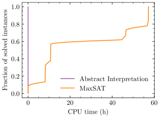
Figure 3: Progression of the MaxSAT and Abstract Interpretation approach when computing minimal explanations, where the depth of trees are doubled compared to the original experiments presented by ? (?).

6.1.2 Minimum Explanations

To assess the runtime performance of Algorithm 7, we again reuse datasets and models from ? (?), and now aim to compute explanations that are minimum with respect to the cost function $g(I;W)=\sum_{i\in I}w_{i}$. Due to lack of domain knowledge in the many different datasets, however, we use the default weighs $W=\{1\}^{n}$, hence $g(I;W)=|I|$. As a baseline for comparison, we implement an alternative algorithm as formalized in Appendix B, which is based on a branch and bound approach realized in some SMT solvers (e.g., ?), and recently used for computing a minimum explanation in the context of neural networks (?). Both algorithms are invoked by a program capable of analyzing several predictions in parallel, where each analysis is configured to abort after an hour. We execute the program on a compute cluster running CentOS 7.8.2003, where each compute node is equipped with an Intel Xeon Gold 6130 processor with 32 CPU cores. A burnup chart of the two approaches is presented in Figure 4, which illustrates the fraction between the number of computed minimum explanations and the number of predictions subject to explanation after a certain amount of accumulated CPU thread time.

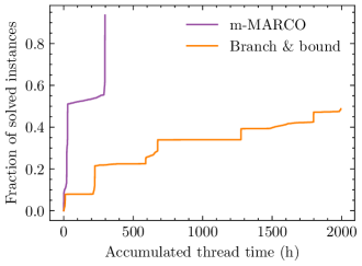
Figure 4: Progression of the branch & bound approach (Algorithm 9) and the m-MARCO approach (Algorithm 7) when computing minimum explanations in parallel.

Clearly, the m-MARCO approach (Algorithm 7) is significantly faster than the one based on branch and bound (Algorithm 9), finding a minimum explanation for about 94% of the problem instances in 297 hours, compared to 49% in 1994 hours, respectively.

6.1.3 Enumerating All Minimal Explanations

To gain further insights on the performance of the m-MARCO approach, we implement the standard MARCO approach (Algorithm 3) that enumerates all minimal explanations, and execute the same experiments on the same compute cluster as before. Figure 5 illustrates a burnup chart in the same format as before, but now comparing Algorithms 3, 6, and 7.

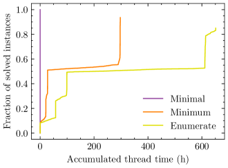
Figure 5: Progress made while computing minimal explanations (Algorithm 6), minimum explanations (Algorithm 7), and when enumerating all minimal explanations (Algorithm 3).

We can clearly see that computing a minimal explanation with Algorithm 6 is significantly faster than computing a minimum explanation with Algorithm 3, which is expected given their theoretical computational complexity being DP-complete and $\Sigma_{2}^{p}$-complete, respectively. We also see that computing a minimum explanation with Algorithm 7 is faster than enumerating all minimal explanations in practice. Overall, we managed to enumerate all minimal explanations for about 85% of the predictions, with an accumulated CPU thread runtime of 651 hours, which is about twice as long as Algorithm 7 which computes a single minimum explanation. For more detailed results, see Appendix C where we list the elapsed runtime and number of timeouts for each individual model.

6.2 Characteristics of Explanations

In this section, we take a closer look at the explanations we enumerated in Section 6.1.3, using the standard MARCO algorithm (Algorithm 3) paired with our valid explanation oracle (Algorithm 5). Note that we are now just interested in the actual explanations, hence the choice of oracle is irrelevant for this study. Any oracle that satisfies Definition 7 (valid explanation oracle) is adequate, which includes all approaches evaluated in Section 6.1.1. First, we investigate the number of (minimal and minimum) explanations that were enumerated for each trained model, and then the number of variables that are present in each computed explanation.

6.2.1 Number of Explanations

Table 3 lists the number of minimal and minimum explanations that were enumerated in Section 6.1.3 using the oracle based on VoTE (Algorithm 5), together with the total number of input variables each model accepts, and how many variables that are referenced during prediction (i.e., $V_{f}$, as defined by Definition 9).

Name of	Input variables		Minimal explanations			Minimum explanations
dataset	referenced	total	min	avg	max	min	avg	max
ann-thyroid	11	21	1	1.5	7	1	1.0	2
appendicitis	7	7	1	7.6	17	1	3.3	11
biodegradation	34	41	1	19,318.8	100,249	1	26.6	466
divorce	14	54	7	126.8	177	1	3.9	19
ecoli	6	7	1	2.4	6	1	2.1	6
glass2	8	9	1	5.9	16	1	2.7	10
ionosphere	31	34	17	25,339.4	102,994	1	18.6	104
pendigits	16	16	6	111.0	263	1	7.0	44
promoters	1	58	1	1.0	1	1	1.0	1
segmentation	17	19	3	40.0	229	1	5.4	38
shuttle	9	9	1	2.6	8	1	1.7	5
sonar	50	60	191	89,407.5	132,654	1	34.5	609
spambase	49	57	7	45,893.6	105,295	1	16.3	215
texture	37	40	987	11,033.3	23,154	1	9.4	105
threeOf9	3	9	1	1.0	1	1	1.0	1
twonorm	20	20	1	2,530.6	17,682	1	21.7	607
vowel	13	13	1	11.7	40	1	3.8	19
wdbc	27	30	3	6,971.3	39,889	1	9.0	70
wine-recognition	12	13	1	5.1	14	1	2.4	6
wpbc	32	33	43	26,629.4	108,520	1	15.9	267
zoo	13	16	1	4.1	10	1	2.0	6

Table 3: Characteristics of input variables of models trained on different datasets, together with the number of minimal and minimum explanations enumerated using the standard MARCO approach (Algorithm 3 combined with Algorithm 5).

We can clearly see that the number of explanations varies greatly, both between different models and between different predictions made by the same model. We also see that the number of referenced variables seems to have a large impact on the average (avg) and maximal (max) number of explanations computed for a particular prediction. In several cases, there are more than 100,000 minimal explanations to choose from. Furthermore, we see that there are significantly fewer minimum than minimal explanations, often by several orders of magnitude. In the most extreme case (the sonar dataset), there are 50 referenced variables, up to 132,654 minimal explanations for a single prediction, and up to 609 minimum explanations. Another insight is that there are several models in which very few of the possible variables are actually used in predictions (i.e. referenced by the model). The extreme case is promoters that uses only one variable out of the 58 possible variables were used in predictions.

6.2.2 Verbosity of Explanations

Figure 6 illustrates a boxplot with costs associated with the verbosity of minimal and minimum explanations for a given model, computed using the cost function $g(I)=|I|$. The figure also illustrates the number of referenced variables in each model with filled circular data points, i.e., $g(V_{f})$.

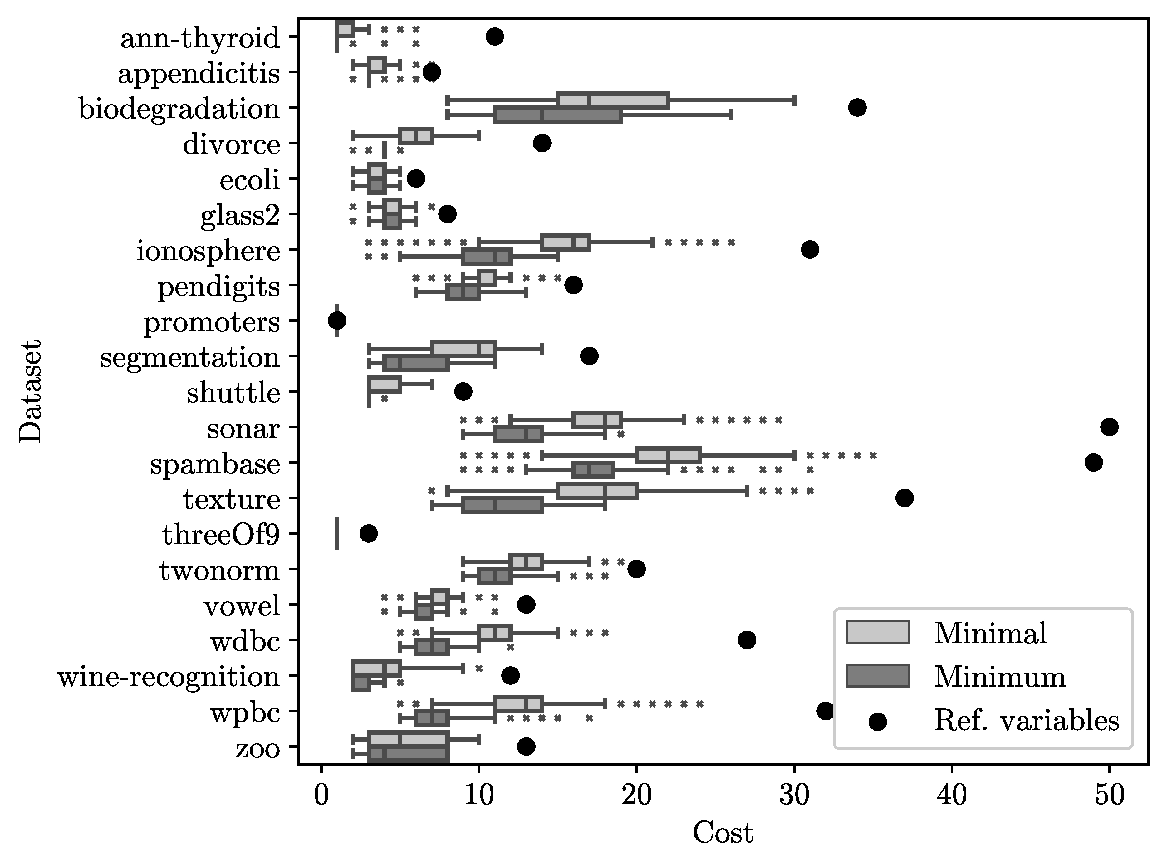
Figure 6: A boxplot illustrating costs of different explanations.

Again, we observe that models with few referenced variables stand out. The threeOf9 model refers to three variables, but all explanations enumerated in our experiments contains a single variable. The promoters model only references a single input variable during prediction, hence all explanations for those prediction cost the same. These are models that provide fewer insights in terms of minimization. The rest of the chart illustrates that significant insights regarding the characteristics of a model can be obtained by performing computations of minimal and minimum explanations. Recall that a circular data point reveals the number of variables in a trivial (verbose) explanation from a model. Then the gap between the circles and the median values for each model reveals that minimization of explanations pays off in terms of verbosity, but the nature of the model dictates the size of the gap. By cross-referencing with Table 3, we can also see that models that yield large numbers of minimal explanations typically have a large spread of the cost associated with them, e.g., the biodegradation and the sonar model. In these cases, we can also see a significant difference in costs when comparing minimal and minimum explanations.

7 Conclusions

When predictions made by machine learning models are used for decision support in critical systems operated by humans, explanations can help the operators to make informed interventions of autonomous actions when explanations appear unjustified. In this context, the explanations must be correct, and preferably without redundant information. The goal of this work has been to provide such explanations efficiently. To this end, we have formalized a sound and complete reasoning engine based on abstract interpretation, tailored specifically for determining the validity of explanations for predictions made by tree ensembles. The reasoning engine is composed of an oracle that can determine the validity of explanations, which is paired with state-of-art algorithms (deletion filter and MARCO) to compute and enumerate minimal explanations. Furthermore, we have presented a novel adaptation of the MARCO algorithm called m-MARCO to compute an explanation that is minimum with respect to a cost function. We demonstrate runtime performance speedups by several orders of magnitude compared to current state-of-the-art. We also show that, in the presence of a highly efficient oracle, it is possible to compute a minimum explanation for several non-trivial tree ensembles. Through enumeration of all minimal explanation, we were able to examine the nature of the obtained explanations. For example, we show that there are typically a large number of minimal explanations to choose from, sometimes exceeding 100,000 for a single prediction. In these cases, we learned that minimum explanations are typically significantly less verbose than minimal explanations, but also more time-consuming to compute. We have also learned that some fundamental algorithms that off-the-shelf constraint solvers rely on can be tailored to narrower classes of problems, in favor of significant increases in runtime performance, thus facilitating computer-aided problem solving that was previously intractable. Our analysis of models in multiple applications from the literature shows that the models in themselves often have superfluous variables, which would appear in explanations without systematic minimization. While some works may aim to improve models by removing unused features, a gap still remains between the features actually used in a model and the least verbose explanations for a given prediction. This gap motivates striving for correct and compact explanations using approaches like ours. As machine learning models mature into well-established and standardized architectures, and their applications become more critical to society, we believe there is a lot to gain by continuing this line of research to include even more types of models and prediction functions, where generic constraint solvers are likely to serve as essential oracles when validating implementations of model-specific ones.

Acknowledgments

This work was partially supported by the Wallenberg AI, Autonomous Systems and Software Program (WASP) funded by the Knut and Alice Wallenberg Foundation. Some computing resources were provided by the Swedish National Infrastructure for Computing (SNIC) and the Swedish National Supercomputer Centre (NSC).

A Oracle for Multi-class Classifiers

For readability, Section 5 only consider explanations for binary classifications. In this section, we define an oracle that reason about collections of tree ensemble, which we used to minimize explanations of predictions made by one-vs-rest classifiers in Section 6. This oracle is formalized as Algorithm 8, and accepts three inputs; a collection of tree ensembles $C$, a set of intervals $\widehat{X}\in\mathcal{I}^{n}$, and the predicted decision $d\in\{1,\ldots,m\}$.

Algorithm 8 Check that a collection of tree ensembles $F_{1},\ldots,F_{m}$ trained on a multi-class classification problem using the one vs. rest paradigm maps all points captured by the abstract input tuple $\widehat{X}=(\widehat{x}_{1},\ldots,\widehat{x}_{n})$ to the label $d\in\{1,\ldots,m\}$, where $m$ is the number of classes.

1:function Multi_Is_Valid($C,\widehat{X},d$)

2:     function $pc_{d}$($\widehat{X}_{d},\widehat{y}_{d}$)

3:         function $pc_{i}$($\widehat{X}_{i},\widehat{y}_{i}$)

4:              $D$ $\leftarrow$ $\gamma(\widehat{y}_{d}>\widehat{y}_{i})$

5:              if $|D|\neq 1$ then

6:                  return $Unsure$

7:              else if $1\in D$ then

8:                  return $Pass$

9:              end if

10:              return $Fail$

11:         end function

12:         for each $i\in\{1\ldots m\}\backslash\{d\}$ do

13:              $o$ $\leftarrow$ VoTE($F_{i},\widehat{X}_{d},pc_{i}$)

14:              if $o\neq Pass$ then

15:                  return $o$

16:              end if

17:         end for

18:         return $Pass$

19:     end function

20:     return VoTE($F_{d},\widehat{X},pc_{d}$) = $Pass$

21:end function

The algorithm defines two nested property checkers ($pc_{d}$ and $pc_{i}$), the latter nested inside the former. Execution of the algorithm starts at line 22, where VoTE is invoked with the $d$-th tree ensemble, the given abstract input tuple $\widehat{X}$, and the outmost property checker $pc_{d}$ (defined on lines 2–18). Once invoked, VoTE will apply its abstraction-refinement approach, and invoke $pc_{d}$ with pairs $(\widehat{X}_{d},\widehat{y}_{d})$ such that $\widehat{X}_{d}\sqsubseteq\widehat{X}$, and $\widehat{y}_{d}=\widehat{f}(\widehat{X}_{d};F_{d})$. Next, execution continues on line 12. Here, all tree ensembles except $F_{d}$ are enumerated, and VoTE is invoked again (line 13), now with each enumerated tree ensemble $F_{i}$, the input region $\widehat{X}_{d}$, and the second property checker $pc_{i}$ (defined on lines 3–11). VoTE will apply its abstraction-refinement approach yet again, but now invoking $pc_{i}$ with pairs $(\widehat{X}_{i},\widehat{y}_{i})$ such that $\widehat{X}_{i}\sqsubseteq\widehat{X}_{d}\sqsubseteq\widehat{X}$, and $\widehat{y}_{i}=\widehat{f}(\widehat{X}_{i};F_{i})$. Inside $pc_{i}$ (lines 3–11), we compare the abstract output of the $i$-th ensemble with $d$-th (line 4). If the comparison is inconclusive, we return $Unsure$, if it is True, we return $Pass$, otherwise we return $Fail$. Back at line 14, we check the outcome the most recent invocation to VoTE. If the outcome is $Fail$, there are some inputs captured by $\widehat{X}$ where the $i$-th tree ensemble predicts a larger value than the $d$-th ensemble, in which case the oracle returns $False$. If the outcome is unsure, we instruct VoTE to further refine $\widehat{X}_{d}$. Otherwise, we continue with the remaining tree ensembles. Figure 7 illustrates a sequence diagram, describing how the different functions in the oracle interact with each other when all property checkers return $Pass$.

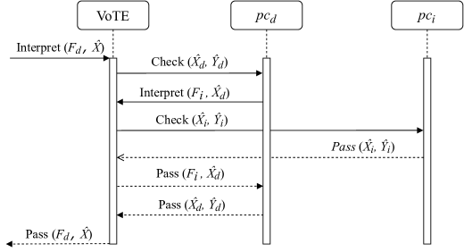
Figure 7: A sequence diagram exemplifying how functions are invoked (solid arrows) and returned from (dashed arrows) in Algorithm 8 when all property checkers return $Pass$. Text associated with arrows describe an action taking place at a particular point in the sequence, with parameters enclosed by parentheses.

B Minimum Explanations using Branch and Bound

In this section, we present an additional algorithm that can compute explanations that are minimum with respect to $g(I;W)=\sum_{i\in I}w_{i}$, where $I\subseteq\{1,\ldots,n\}$ and $W\in\mathbb{R}_{\geq 0}^{n}$. This algorithm is based on a branch and bound approach realized in some SMT solvers (e.g., ?), and recently used for computing a minimum explanation in the context of neural networks (?). Algorithm 9 starts by initializing an explanation $I_{cur}$ with the indices of all variables referenced by the ensemble (line 1). It then initializes a tuple $(\widehat{x}_{1},\ldots,\widehat{x}_{n})$ that captures the entire concrete input domain (line 2). Next, a nested and recursive branch-and-bound procedure is defined (lines 4–16) that takes two input parameters; a set of indices $I$ of explanation variables, and a new index $i$ to be added to this set. In this procedure, we start by adding the index $i$ to the set $I$ (line 5), and then bound the search for explanations to those that cost less than the current candidate $I_{cur}$ using the cost function $g$ (lines 6–8). If the cost $g(I)$ is greater than the cost $g(I_{cur})$, we simply return from the procedure. Otherwise, we refine the $i$-th abstraction to capture precisely the $i$-th concrete input value (line 9). We then query the oracle to see if all concrete values captured by the updated $(\widehat{x}_{1},\ldots,\widehat{x}_{n})$ map to the same label (line 10). If that is the case, we have found a cheaper explanation which we assign to $I_{cur}$ (line 11). Otherwise, we permutate over remaining referenced variable indices not in $I$ by invoking the recursive procedure (lines 13–15). Finally, the abstraction $\widehat{x}_{i}$ is restored (line 17). With the branch-and-bound procedure defined, we start the minimization of the current candidate $I_{cur}$ by sequentially invoking the procedure with indices of variables referenced by the tree ensemble (lines 18–20). Finally, we return $I_{cur}$ (line 22).

Algorithm 9 A branch and bound approach for computing an explanation that is minimum with respect to the cost function $g$ for a tree ensemble $F$ and input sample $c_{1},\ldots,c_{n}$, classified as label $d$.

1:function Minimum_Explanation($F,V_{f},c_{1},\ldots,c_{n},d,W=\{1\}^{n}$)

2:     $I_{cur}$ $\leftarrow$ $V_{f}$ $\triangleright$ Initialize current explanation to the most expensive

3:     $\widehat{x}_{1},\ldots,\widehat{x}_{n}$ $\leftarrow$ $\top,\ldots,\top$ $\triangleright$ Relax all variables

4:     procedure Add_Variable($I,i$) $\triangleright$ Define recursive branch-and-bound procedure

5:         $I$ $\leftarrow$ $I\cup\{i\}$ $\triangleright$ Add index $i$ to set of indices $I$

6:         if $g(I_{cur};W)\leq g(I;W)$ then $\triangleright$ Bound the search

7:              return

8:         end if

9:         $\widehat{x}_{i}$ $\leftarrow$ $\alpha(\{c_{i}\})$ $\triangleright$ Assign value to the $i$-th variable

10:         if Is_Valid($F,(\widehat{x}_{1},\ldots,\widehat{x}_{n}),d$) then $\triangleright$ Query the oracle

11:              $I_{cur}$ $\leftarrow$ $I$ $\triangleright$ Found a cheaper explanation

12:         else

13:              for each $j\in V_{f}\backslash I$ do $\triangleright$ Branch on remaining indices

14:                  Add_Variable($I,j$)

15:              end for

16:         end if

17:         $\widehat{x}_{i}$ $\leftarrow$ $\top$ $\triangleright$ Relax the $i$-th variable again

18:     end procedure

19:     for each $i\in V_{f}$ do $\triangleright$ Start minimizing $I_{cur}$

20:         Add_Variable($\emptyset,i$)

21:     end for

22:     return $I_{cur}$ $\triangleright$ Return the set of indices in the explanation

23:end function

C Detailed Performance Results

In this section, we provide information on the runtime performance of algorithms evaluated in Section 6, but here for each individual model. In particular, Table 4 lists performance of the branch and bound based algorithm for computing a single minimum explanation (Algorithm 9), Table 5 for the m-MARCO approach for computing a single minimum explanation (Algorithm 7), and Table 6 for the standard MARCO approach (Algorithm 3) which enumerates all minimal explanations.

Name of	Input variables		Runtime (s)			Number of
dataset	referenced	total	min	avg	max	timeouts
ann-thyroid	11	21	0.88	18.54	3202.54	10
appendicitis	7	7	0.00	0.02	0.25	0
biodegradation	34	41	–	–	–	200
divorce	14	54	0.33	208.35	914.47	4
ecoli	6	7	0.04	0.35	2.46	0
glass2	8	9	0.00	0.18	1.64	0
ionosphere	31	34	1.31	404.95	3200.84	162
pendigits	16	16	–	–	–	200
promoters	1	58	0.00	0.00	0.00	0
segmentation	17	19	0.13	343.79	3465.32	74
shuttle	9	9	0.04	0.35	1.56	0
sonar	50	60	–	–	–	200
spambase	49	57	–	–	–	200
texture	37	40	–	–	–	200
threeOf9	3	9	0.00	0.00	0.00	0
twonorm	20	20	–	–	–	200
vowel	13	13	35.76	1256.71	3575.15	109
wdbc	27	30	667.14	1094.42	3565.04	173
wine-recognition	12	13	0.03	1.51	18.61	0
wpbc	32	33	387.06	687.63	1729.96	182
zoo	13	16	0.07	101.15	1197.41	11

Table 4: Runtime performance of Algorithm 9 when computing minimum explanations.

Name of	Input variables		Runtime (s)			Number of
dataset	referenced	total	min	avg	max	timeouts
ann-thyroid	11	21	0.02	0.07	0.15	0
appendicitis	7	7	0.00	0.02	0.05	0
biodegradation	34	41	0.02	242.65	3384.13	8
divorce	14	54	0.04	0.17	0.35	0
ecoli	6	7	0.01	0.04	0.08	0
glass2	8	9	0.01	0.03	0.06	0
ionosphere	31	34	0.07	115.58	1395.78	0
pendigits	16	16	0.37	4.16	15.59	0
promoters	1	58	0.00	0.00	0.00	0
segmentation	17	19	0.01	0.26	1.59	0
shuttle	9	9	0.01	0.03	0.10	0
sonar	50	60	0.59	724.90	3246.32	126
spambase	49	57	0.13	501.80	3298.29	108
texture	37	40	3.27	122.20	2140.48	0
threeOf9	3	9	0.00	0.00	0.01	0
twonorm	20	20	0.04	7.90	41.29	0
vowel	13	13	0.08	0.48	1.35	0
wdbc	27	30	0.07	3.03	16.35	0
wine-recognition	12	13	0.01	0.04	0.09	0
wpbc	32	33	0.24	12.79	110.41	0
zoo	13	16	0.01	0.05	0.12	0

Table 5: Runtime performance of Algorithm 7 when computing minimum explanations.

Name of	Input variables		Runtime (s)			Number of
dataset	referenced	total	min	avg	max	timeouts
ann-thyroid	11	21	0.00	0.02	0.18	0
appendicitis	7	7	0.00	0.02	0.05	0
biodegradation	34	41	0.00	277.99	2925.64	42
divorce	14	54	0.02	0.28	0.45	0
ecoli	6	7	0.00	0.03	0.11	0
glass2	8	9	0.00	0.02	0.06	0
ionosphere	31	34	0.00	202.22	3029.13	29
pendigits	16	16	0.61	25.30	92.84	0
promoters	1	58	0.00	0.00	0.01	0
segmentation	17	19	0.03	1.47	11.24	0
shuttle	9	9	0.00	0.04	0.18	0
sonar	50	60	0.00	138.15	3555.12	160
spambase	49	57	0.00	156.06	3310.70	151
texture	37	40	0.00	357.77	3586.91	166
threeOf9	3	9	0.00	0.00	0.00	0
twonorm	20	20	0.00	15.21	155.54	0
vowel	13	13	0.02	0.90	4.85	0
wdbc	27	30	0.01	38.42	420.70	0
wine-recognition	12	13	0.00	0.04	0.16	0
wpbc	32	33	0.00	400.56	3440.58	16
zoo	13	16	0.00	0.04	0.12	0

Table 6: Runtime performance of Algorithm 3 when enumerating minimal explanations.

References

- Audemard et al. Audemard, G., Bellart, S., Bounia, L., Koriche, F., Lagniez, J.-M., and Marquis, P. (2022). Trading complexity for sparsity in random forest explanations. In Proceedings of the Thirty-Sixth AAAI Conference on Artificial Intelligence. AAAI Press.
- Boumazouza et al. Boumazouza, R., Cheikh-Alili, F., Mazure, B., and Tabia, K. (2021). ASTERYX: A Model-Agnostic SaT-BasEd AppRoach for SYmbolic and Score-Based EXplanations, p. 120–129. Association for Computing Machinery, New York, NY, USA.
- Brain et al. Brain, M., Tinelli, C., Rümmer, P., and Wahl, T. (2015). An automatable formal semantics for ieee-754 floating-point arithmetic. In 2015 IEEE 22nd Symposium on Computer Arithmetic, pp. 160–167. IEEE.
- Breiman Breiman, L. (2001). Random forests. Machine learning, 45(1), 5–32.
- Chen and Guestrin Chen, T., and Guestrin, C. (2016). Xgboost: A scalable tree boosting system. In Proceedings of the 22nd ACM SIGKDD International Conference on Knowledge Discovery and Data Mining, KDD ’16, p. 785–794, New York, NY, USA. Association for Computing Machinery.
- Chinneck and Dravnieks Chinneck, J. W., and Dravnieks, E. W. (1991). Locating minimal infeasible constraint sets in linear programs. ORSA Journal on Computing, 3(2), 157–168.
- Cousot and Cousot Cousot, P., and Cousot, R. (1977). Abstract interpretation: A unified lattice model for static analysis of programs by construction or approximation of fixpoints. In Proceedings of the 4th ACM SIGACT-SIGPLAN symposium on Principles of Programming Languages (POPL), pp. 238–252, Los Angeles, California. ACM Press, New York, NY.
- Darwiche and Hirth Darwiche, A., and Hirth, A. (2020). On the reasons behind decisions. In In Proceedings of the 24th European Conference on Artificial Intelligence (ECAI), pp. 712–720. IOS Press.
- Dillig et al. Dillig, I., Dillig, T., McMillan, K. L., and Aiken, A. (2012). Minimum satisfying assignments for smt. In International Conference on Computer Aided Verification, pp. 394–409. Springer.
- Friedman Friedman, J. H. (2001). Greedy function approximation: A gradient boosting machine. The Annals of Statistics, 29(5), 1189–1232.
- Gunning et al. Gunning, D., Vorm, E., Wang, J. Y., and Turek, M. (2021). DARPA’s explainable AI (XAI) program: A retrospective. Applied AI Letters, 2(4).
- Hadji Misheva et al. Hadji Misheva, B., Jaggi, D., Posth, J.-A., Gramespacher, T., and Osterrieder, J. (2021). Audience-dependent explanations for ai-based risk management tools: A survey. Frontiers in Artificial Intelligence, 4.
- Ignatiev et al. Ignatiev, A., Izza, Y., Stuckey, P. J., and Marques-Silva, J. (2022). Using maxsat for efficient explanations of tree ensembles. In Proceedings of the Thirty-Sixth AAAI Conference on Artificial Intelligence. AAAI Press.
- Ignatiev and Marques-Silva Ignatiev, A., and Marques-Silva, J. (2021). Sat-based rigorous explanations for decision lists. In Li, C.-M., and Manyà, F. (Eds.), Theory and Applications of Satisfiability Testing – SAT 2021, pp. 251–269, Cham. Springer International Publishing.
- Ignatiev et al. Ignatiev, A., Narodytska, N., and Marques-Silva, J. (2019). Abduction-based explanations for machine learning models. In Proceedings of the AAAI Conference on Artificial Intelligence, Vol. 33, pp. 1511–1519.
- Ignatiev et al. Ignatiev, A., Previti, A., and Marques-Silva, J. (2016). On finding minimum satisfying assignments. In International Conference on Principles and Practice of Constraint Programming, pp. 287–297. Springer.
- Irsoy et al. Irsoy, O., Yildiz, O. T., and Alpaydin, E. (2012). Soft decision trees. In International Conference on Pattern Recognition. IEEE.
- Izza et al. Izza, Y., Ignatiev, A., and Marques-Silva, J. (2022). On tackling explanation redundancy in decision trees. Journal of Artificial Intelligence Research, 75, 61–321.
- Izza and Silva Izza, Y., and Silva, J. M. (2021). On explaining random forests with sat. In 30th International Joint Conference on Artificial Intelligence. International Joint Conferences on Artifical Intelligence (IJCAI).
- Kaur et al. Kaur, D., Uslu, S., Rittichier, K. J., and Durresi, A. (2022). Trustworthy artificial intelligence: A review. ACM Computing Surveys (CSUR), 55(2), 1–38.
- La Malfa et al. La Malfa, E., Zbrzezny, A., Michelmore, R., Paoletti, N., and Kwiatkowska, M. (2021). On guaranteed optimal robust explanations for nlp models. In 30th International Joint Conference on Artificial Intelligence, pp. 2658–2665. International Joint Conferences on Artifical Intelligence (IJCAI).
- Liffiton and Malik Liffiton, M. H., and Malik, A. (2013). Enumerating infeasibility: Finding multiple MUSes quickly. In International Conference on Integration of Constraint Programming, Artificial Intelligence, and Operations Research, pp. 160–175. Springer.
- Liffiton et al. Liffiton, M. H., Previti, A., Malik, A., and Marques-Silva, J. (2016). Fast, flexible mus enumeration. Constraints, 21(2), 223–250.
- Marques-Silva et al. Marques-Silva, J., Gerspacher, T., Cooper, M. C., Ignatiev, A., and Narodytska, N. (2021). Explanations for monotonic classifiers. In International Conference on Machine Learning, pp. 7469–7479. PMLR.
- Marquis Marquis, P. (1991). Extending abduction from propositional to first-order logic. In International Workshop on Fundamentals of Artificial Intelligence Research, pp. 141–155. Springer.
- Pedregosa et al. Pedregosa, F., Varoquaux, G., Gramfort, A., Michel, V., Thirion, B., Grisel, O., Blondel, M., Prettenhofer, P., Weiss, R., Dubourg, V., et al. (2011). Scikit-learn: Machine learning in Python. Journal of machine learning research, 12, 2825–2830.
- Previti and Marques-Silva Previti, A., and Marques-Silva, J. (2013). Partial mus enumeration. In Twenty-Seventh AAAI Conference on Artificial Intelligence.
- Prokhorenkova et al. Prokhorenkova, L., Gusev, G., Vorobev, A., Dorogush, A. V., and Gulin, A. (2018). Catboost: unbiased boosting with categorical features. In Advances in Neural Information Processing Systems (NIPS).
- Quine Quine, W. V. (1952). The problem of simplifying truth functions. The American mathematical monthly, 59(8), 521–531.
- Ranzato and Zanella Ranzato, F., and Zanella, M. (2020). Abstract interpretation of decision tree ensemble classifiers. In Proceedings of the Thirty-Fourth AAAI Conference on Artificial Intelligence, pp. 5478–5486. AAAI Press.
- Ras et al. Ras, G., Xie, N., van Gerven, M., and Doran, D. (2022). Explainable deep learning: A field guide for the uninitiated. Journal of Artificial Intelligence Research, 73, 329–397.
- Shih et al. Shih, A., Choi, A., and Darwiche, A. (2018). A symbolic approach to explaining bayesian network classifiers. In Proceedings of the 27th International Joint Conference on Artificial Intelligence, pp. 5103–5111.
- Shih et al. Shih, A., Choi, A., and Darwiche, A. (2019). Compiling bayesian network classifiers into decision graphs. In Proceedings of the AAAI Conference on Artificial Intelligence, Vol. 33, pp. 7966–7974.
- Shwartz-Ziv and Armon Shwartz-Ziv, R., and Armon, A. (2022). Tabular data: Deep learning is not all you need. Information Fusion, 81, 84–90.
- Törnblom and Nadjm-Tehrani Törnblom, J., and Nadjm-Tehrani, S. (2019). An abstraction-refinement approach to formal verification of tree ensembles. In International Conference on Computer Safety, Reliability, and Security (SAFECOMP), pp. 301–313. Springer.
- Törnblom and Nadjm-Tehrani Törnblom, J., and Nadjm-Tehrani, S. (2021). Scaling up memory-efficient formal verification tools for tree ensembles. arXiv preprint, arXiv:2105.02595.
- Wang et al. Wang, F., Wang, Q., Nie, F., Yu, W., and Wang, R. (2018). Efficient tree classifiers for large scale datasets. Neurocomputing, 284.