Magnetic-field-induced corner states in quantum spin Hall insulators

Abstract

We address the general problem of magnetic-field-induced corner states in quantum spin Hall insulators (QSHIs). Our analytical findings reveal that when applied to the QSHIs in zinc-blende semiconductor quantum wells (QWs), the presence of corner states extends beyond the anticipated range of meeting edges, surpassing the limitations imposed by crystal symmetry. We clearly demonstrate that, in the most general scenario, magnetic field-induced corner states in QSHIs are not topological. However, we find that the presence of crystal symmetry can stabilize these states only under specific orientations of the in-plane magnetic field and meeting edges. Therefore, contrary to previous assumptions, our research unveils that QSHIs in the presence of a magnetic field cannot be accurately considered as higher-order topological insulators. Furthermore, the lack of an inversion center in zinc-blende semiconductor QWs enables the emergence of corner states through the influence of a perpendicular magnetic field.

Introduction.– Recently, a novel classification of topological systems has led to the discovery of higher-order topological insulators (HOTIs) Benalcazar et al. (2017); Langbehn et al. (2017a); Song et al. (2017); Schindler et al. (2018a); Ezawa (2018a). While conventional (first-order) $m$-dimensional topological insulators Kane and Mele (2005); Bernevig et al. (2006); König et al. (2007); Hasan and Kane (2010); Qi and Zhang (2011); Bansil et al. (2016) exhibit gapless states at their ($m-1$)-dimensional boundaries, $n$th-order $m$-dimensional topological insulator possesses gapless edge states at its ($m-n$)-dimensional boundaries. To date, HOTI state has been observed in bismuth Schindler et al. (2018b), WTe₂ Choi et al. (2020), bismuth-halide chains Noguchi et al. (2021), Bi₄Br₄ Shumiya et al. (2022) and predicted in many other systems including bulk crystals and QWs Wang et al. (2019); Ezawa (2018b); Sheng et al. (2019); Park et al. (2019); Fang and Cano (2020); Krishtopenko (2021). Similarly, the conception of higher-order topology can also be applied to photonic Chen et al. (2019); Hassan et al. (2019); Kim et al. (2020) and acoustic crystals Xue et al. (2019); Ni et al. (2019); He et al. (2019), topoelectrical-circuits Imhof et al. (2018); Serra-Garcia et al. (2019); Bao et al. (2019); Ezawa (2019) and superconductors Langbehn et al. (2017b); Khalaf (2018); Wang et al. (2018); Yan et al. (2018); Yan (2019).

As previously believed, one of the widespread way to construct HOTI state is to consider a conventional topological system of specific crystal symmetry and to break time reversal symmetry. Particularly, such a mechanism of the realization of corner states was demonstrated for QSHIs described within square Ezawa (2018c) and honeycomb Ezawa (2018c); Ren et al. (2020); Chen et al. (2020) lattice models preserving an electron-hole symmetry even in the presence of magnetic field. It is worth noting that electron-hole symmetry, considered one of the most robust symmetries in condensed matter physics, can effectively conceal crystal symmetry-related effects of QSHIs. A striking example of realistic QSHIs without an electron-hole symmetry are the QSHIs based on zinc-blende semiconductor QWs, like HgTe/CdTe Bernevig et al. (2006); König et al. (2007) and InAs/Ga(In)Sb quantum wells (QWs) Liu et al. (2008); Knez et al. (2011); Krishtopenko and Teppe (2018); Krishtopenko et al. (2018, 2019); Schmid et al. (2022); Avogadri et al. (2022) The concrete choice of QSHI is also crucial for the Zeeman field, which depends on the crystal symmetry and may also not possess an electron-hole symmetry.

Within this paper, we provide an analytical solution to the general problem of magnetic field-induced corner states in QSHIs, specifically focusing on scenarios where electron-hole symmetry is absent. Our findings for zinc-blende QSHIs demonstrate the existence of localized states induced by in-plane magnetic field at the corners, including those that do not locally preserve a crystal symmetry. This means that the corner states in the latter case are not topological, and QSHI in the presence of a magnetic field cannot be strictly classified as HOTI. Importantly, due to the absence of an inversion center, the corner states in zinc-blende semiconductor QWs can be also induced by a perpendicular magnetic field. We also note that our analytical results, being applied to the QSHIs treated within the lattice models Ezawa (2018c); Ren et al. (2020); Chen et al. (2020), perfectly reproduce and extend understanding of the results previously obtained by numerical calculations.

Hamiltonian for zinc-blende QSHIs.– First, we focus on prototype zinc-blende semiconductor QW with symmetric heteropotential grown along the $z||[001]$ axis. The low-energy Hamiltonian of such systems for the electron-like $E1$ and heavy-hole-like $H1$ subbands, written in the basis $|E1{\uparrow}\rangle$, $|H1{\uparrow}\rangle$, $|E1{\downarrow}\rangle$, $|H1{\downarrow}\rangle$, has the form Bernevig et al. (2006):

$$H_{\mathrm{2D}}(\mathbf{k})=\begin{pmatrix}H_{\mathrm{BHZ}}(\mathbf{k})&-i\Delta{e^{-2i\theta}}\sigma_{y}\\ i\Delta{e^{2i\theta}}\sigma_{y}&H_{\mathrm{BHZ}}^{*}(-\mathbf{k})\end{pmatrix},$$ (1)

where asterisk stands for complex conjugation, $\mathbf{k}=(k_{x},k_{y})$ is the momentum in the plane, and $H_{\mathrm{BHZ}}(\mathbf{k})=\epsilon_{k}+d_{a}(\mathbf{k})\sigma_{a}$. Here, $\sigma_{a}$ are the Pauli matrices acting in the “basis” space, $\epsilon_{k}=C-\mathbb{D}k^{2}$, $d_{1}(\mathbf{k})=Ak_{x}$, $d_{2}(\mathbf{k})=Ak_{y}$, $d_{3}(k)=M-\mathbb{B}k^{2}$ and $k^{2}=k_{x}^{2}+k_{y}^{2}$. The mass parameter $M$ describes the inversion between the electron-like E1 and the hole-like H1 subbands: $M>0$ corresponds to a trivial state, while $M<0$ is for QSHI Bernevig et al. (2006). The non-diagonal terms in $H_{\mathrm{2D}}(\mathbf{k})$ proportional to $\Delta$ describe the joint effect of bulk inversion asymmetry (BIA) of the unit cell of zinc-blende semiconductors Dresselhaus (1955) and the interface inversion asymmetry (IIA) of the QW Ivchenko et al. (1996); Durnev and Tarasenko (2016). Experimental results known from the literature show that the values of $\Delta$ are small in HgTe/CdTe QWs Büttner et al. (2011); Kadykov et al. (2018); Brüne et al. (2012); Kadykov et al. (2015, 2016); Olshanetsky et al. (2018); Yahniuk et al. (2019); Krishtopenko et al. (2020), while they can be relatively large in InAs/GaInSb-based heterostructures Olesberg et al. (2001); Szmulowicz et al. (2004); Li et al. (2010); Lang and Xia (2011); Dong et al. (2015); Chen et al. (2016).

In $H_{\mathrm{2D}}(\mathbf{k})$, $\theta$ is the angle between the $x$ axis and the (001) crystallographic direction (see Fig. 1). This coordinate system allows one to consider the edge states with different crystallographic orientations of the edge. To obtain $H_{\mathrm{2D}}(\mathbf{k})$ in Eq. (1) from a Hamiltonian with $\theta=0$, together with a clock-wise rotation of the coordinate system along $z$ axis, it is also necessary to perform a unitary transformation of the Hamiltonian given by $U=\exp(-i\theta{J_{\xi}})$. Here, $J_{\xi}$ is a diagonal matrix with the elements $(1/2,3/2,-1/2,-3/2)$ corresponding to the momentum of the basis states $|E1{\uparrow}\rangle$, $|H1{\uparrow}\rangle$, $|E1{\downarrow}\rangle$, $|H1{\downarrow}\rangle$, respectively Bernevig et al. (2006).

In order to take into account effect of in-plane magnetic field $\mathbf{B}$, one has to make the Peierls substitution $\mathbf{k}\rightarrow\mathbf{k}-(e/c\hbar)\mathbf{A}$ in $H_{\mathrm{2D}}(\mathbf{k})$ and to add the Zeeman Hamiltonian:

$$H_{\mathrm{Z}}=\dfrac{\mu_{B}}{2}\begin{pmatrix}0&0&g_{e}^{||}B_{+}&0\\ 0&0&0&g_{h}^{||}e^{-i4\theta}B_{-}\\ g_{e}^{||}B_{-}&0&0&0\\ 0&g_{h}^{||}e^{i4\theta}B_{+}&0&0\end{pmatrix},$$ (2)

where $B_{\pm}=B_{x}{\pm}iB_{y}$, $\mu_{B}$ is the Bohr magneton, $g_{e}^{||}$ and $g_{h}^{||}$ are the in-plane g-factors of the $E1$ and $H1$ subbands, resulting from the bare electron g-factor and the interaction with the remote electron and hole subbands Winkler (2003). Since, one can always choose the vector potential gauge so that $\mathbf{A}||z$ for in-plane magnetic field, we can always restrict ourselves to considering only the Zeeman term omitting the Peierls substitution for $k_{x}$ and $k_{y}$. The angular dependence of $H_{\mathrm{Z}}$ on $\theta$ in the chosen coordinate system is obtained in the same way as for $H_{\mathrm{2D}}(\mathbf{k})$.

As clear, $\Delta$ and $g_{h}^{||}$ are the terms breaking rotational symmetry of $H_{\mathrm{2D}}(\mathbf{k})$ and $H_{\mathrm{Z}}$. They both origin from the contribution of the $\Gamma_{8}$ bulk band of zinc-blende semiconductors Winkler (2003). In the following, we set $\Delta$ and $g_{h}^{||}$ to zero if one needs to “switch off” the crystal symmetry of the prototype (001) QW.

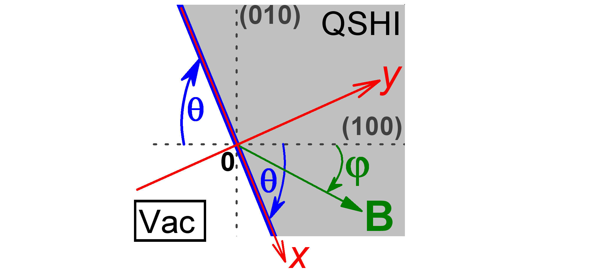
Figure 1: The layout of the coordinate axes (in red) and orientation the magnetic field $B$ (in green) with respect to the main crystallographic axes shown by the vertical and horizontal dashed lines. The QW edge (in blue) considered in the text is oriented along $x$ axis. The positive values of $\theta$ and $\varphi$ correspond to a clockwise rotation around $z$ axis.

Hamiltonian for gapped edge states.– To analyze the existence of corner states, we first need to obtain a 1D edge Hamiltonian. To derive an effective 1D low-energy edge Hamiltonian, we consider a semi-infinite plane $y>0$ with open-boundary conditions at $y=0$ as shown in Fig. 1. Then, we solve the eigenvalue problem for $H_{\mathrm{2D}}(\mathbf{k})$ at $M<0$ to find the edge wave-functions at $k_{x}=0$. Finally, to derive the edge Hamiltonian, one should successively project the part of $H_{\mathrm{2D}}(\mathbf{k})$ with non-zero $k_{x}$ and $H_{\mathrm{Z}}$ onto the calculated edge wave-functions. The procedure described above is fairly standard, so we do not present its details here. Up to our knowledge, in the presence of non-zero $\Delta$, it was first implemented by Durnev et al. Durnev and Tarasenko (2016)

After tedious and routine mathematics, the part of the edge Hamiltonian independent of $\mathbf{B}$ at small values of $k_{x}$ is written as

$$H_{\mathrm{edge}}^{(0)}(k_{x})=\varepsilon_{0}+\hbar{v_{F}}k_{x}{s}_{z}+\mathcal{O}\left(k_{x}^{2}\right),$$ (3)

where $s_{a}$ ($a=x,y,z$) corresponds to the Pauli matrices acting on spin degree of freedom, $\varepsilon_{0}=C-\eta{M}$ and $\hbar{v_{F}}$ is defined as Durnev (2020)

$$\hbar{v_{F}}=A\sqrt{1-\eta^{2}}\Omega,$$ (4)

where $\eta=\mathbb{D}/\mathbb{B}$ and

$$\Omega=\dfrac{|M|\sqrt{1-\eta^{2}}}{\sqrt{\left(1-\eta^{2}\right)M^{2}+\Delta^{2}}}.$$ (5)

Note that the non-linear terms in $k_{x}$ arise in Eq. (3) due to the presence of $\Delta$. They are all vanishing if $\Delta=0$ Durnev (2020).

Similarly, the Zeeman part of the edge Hamiltonian can be presented in the form Durnev and Tarasenko (2016)

$$H_{\mathrm{edge}}^{(\mathbf{B})}=\dfrac{\mu_{B}}{2}\sum_{a,b=x,y}g_{ab}s_{a}B_{\beta},$$ (6)

where the edge g-factor tensor $g_{ab}$ depends on the edge orientation with the following non-zero components:

$$g_{xx}=g_{1}\cos^{2}2\theta+g_{2}\sin^{2}2\theta,~{}$$

$$g_{yy}=g_{1}\sin^{2}2\theta+g_{2}\cos^{2}2\theta,~{}$$

$$g_{xy}=g_{yx}=\dfrac{1}{2}\left(g_{1}-g_{2}\right)\sin{4\theta}.$$ (7)

Here, $g_{1}$ and $g_{2}$ are two constants written as Durnev (2020)

$$g_{1}=g_{e}^{||}\dfrac{1-\eta}{2}+g_{h}^{||}\dfrac{1+\eta}{2},~{}~{}~{}~{}$$

$$g_{2}=\left(g_{e}^{||}\dfrac{1-\eta}{2}-g_{h}^{||}\dfrac{1+\eta}{2}\right)\Omega.$$ (8)

As clear, if one neglects the terms resulting from the crystal symmetry of zinc-blende semiconductors, $g_{1}=g_{2}$, and the g-factor of the edges states becomes independent of the edge orientation.

Assuming that the magnetic field $\mathbf{B}$ is oriented at an angle $\varphi$ to the [100] crystallographic direction as shown in Fig. 1, Eq. (6) is rewritten as

$$H_{\mathrm{edge}}^{(\mathbf{B})}=M_{x}{s}_{x}+M_{y}{s}_{y},$$ (9)

where

$$M_{x}=\dfrac{E_{Z}}{2}\left[g_{+}\cos(\theta-\varphi)+g_{-}\cos(3\theta+\varphi)\right],~{}$$

$$M_{y}=\dfrac{E_{Z}}{2}\left[g_{+}\sin(\theta-\varphi)+g_{-}\sin(3\theta+\varphi)\right]~{}~{}~{}$$ (10)

with $E_{Z}=\mu_{B}g_{1}B/2$ and $g_{\pm}=1\pm{g_{2}/g_{1}}$.

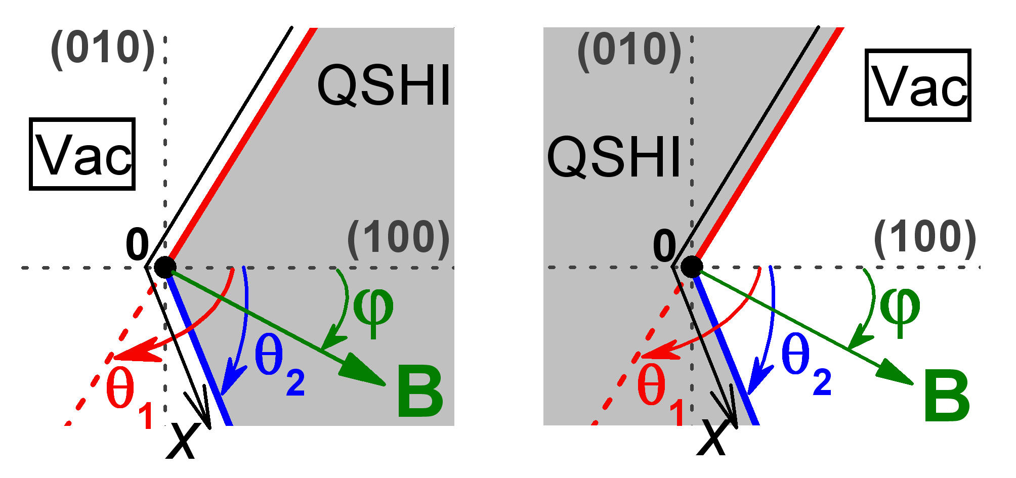
Figure 2: Schematic of orientation of two meeting edges (defined by $\theta_{1}$ and $\theta_{2}$) and magnetic field (defined by $\varphi$) with respect to main crystallographic axes in the QW plane. Here, the “curved” $x$ axis is oriented along the edges so that $x=0$ represents to the meeting corner, while $x<0$ and $x>0$ correspond to $\theta_{1}$ and $\theta_{2}$, respectively. Note that the latter is fulfilled only if $\theta_{1}-\theta_{2}\neq\pm\pi$. The QSHI and external vacuum are shown in grey and white, respectively. The positive values of the angles correspond to a clockwise rotation around $z$ axis. The right and left panels represent the same case considered in the text.

Corner states.– Let us now redefine the coordinate $x$ along the “curved” edge so that $x=0$ corresponds to the meeting corner. The latter means that $M_{x}$ and $M_{y}$ in Eq. (Magnetic-field-induced corner states in quantum spin Hall insulators) are now the functions of $x$, and $\hat{k}_{x}=-i\partial/\partial{x}$. Note that the edge Hamiltonian is defined in disjoint regions out of $x=0$. As a boundary condition at $x=0$, we further assume the continuity of the edge wave-function.

In view of the above, the Schrödinger equation for the corner states takes the form

$$\left({\hbar}v_{F}\hat{k}_{x}{s}_{z}+M_{x}(x){s}_{x}+M_{y}(x){s}_{y}\right)\Psi_{\mathrm{0D}}(x)\\ =\left(E-\varepsilon_{0}\right)\Psi_{\mathrm{0D}}(x).$$ (11)

Let us act by the matrix operator from the left-hand side of Eq. (11) on both sides of this equation. This leads to

$$\bigg{\{}\left({\hbar}^{2}v_{F}^{2}\hat{k}_{x}^{2}+M_{x}^{2}+M_{y}^{2}-\left(E-\varepsilon_{0}\right)^{2}\right)~{}\\ +{\hbar}v_{F}\begin{pmatrix}0&-i{M_{x}}^{\prime}-M_{y}^{\prime}\\ i{M_{x}}^{\prime}-M_{y}^{\prime}&0\end{pmatrix}\bigg{\}}\Psi_{\mathrm{0D}}(x)=0,$$ (12)

where the prime denotes the derivative with respect to $x$.

An exact solution of Eq. (12) can be found in the case of a sharp corner at $x=0$, when

$$M_{x}(x)={\alpha_{x}}\Theta(x)+m_{x},~{}~{}~{}~{}~{}~{}~{}~{}M_{y}(x)={\alpha_{y}}\Theta(x)+m_{y},$$ (13)

where $\Theta(x)$ is a step-function defined as $\Theta(x)=-1$ if $x<0$ and $\Theta(x)=1$ for $x\geq 0$, while the constants ${\alpha_{x}}$, ${\alpha_{x}}$, ${m_{x}}$ and ${m_{y}}$ are written as

$$\alpha_{x,y}=\dfrac{M_{x,y}(+\infty)-M_{x,y}(-\infty)}{2},$$

$$m_{x,y}=\dfrac{M_{x,y}(+\infty)+M_{x,y}(-\infty)}{2}.$$ (14)

Hence, solutions of Eq. (12) is constructed as follows:

$$\Psi_{\mathrm{0D}}(x)={\chi}\psi(x),$$ (15)

where ${\chi}$ is the spin part of the wave function satisfying the equation

$$\begin{pmatrix}0&-\alpha_{y}-i{\alpha_{x}}\\ -\alpha_{y}+i{\alpha_{x}}&0\end{pmatrix}{\chi}=\nu{\chi},$$

with the eigenvalues $\nu=\pm\sqrt{\alpha_{x}^{2}+\alpha_{y}^{2}}$.

By introducing a new variable $\tilde{x}=x/({\hbar}v_{F})$, the equation for the coordinate part $\psi(x)$ can be written as

$$\Bigg{\{}\hat{\tilde{k}}_{x}^{2}+{W}(\tilde{x})^{2}+\sigma{W}(\tilde{x})^{\prime}\Bigg{\}}\psi(\tilde{x})=\varepsilon{\psi}(\tilde{x}),$$ (16)

where $\sigma=\pm{1}$ (the sign of $\sigma$ coincides with those for $\nu$), and $\varepsilon$ and ${W}(\tilde{x})$ are defined as

$$\varepsilon=\left(E-\varepsilon_{0}\right)^{2}-\dfrac{\left(m_{x}\alpha_{y}-m_{y}\alpha_{x}\right)^{2}}{\alpha_{x}^{2}+\alpha_{y}^{2}},$$

$${W}(\tilde{x})=\dfrac{\alpha_{x}M_{x}(\tilde{x})+\alpha_{y}M_{y}(\tilde{x})}{\sqrt{\alpha_{x}^{2}+\alpha_{y}^{2}}}.~{}~{}~{}~{}$$ (17)

Importantly, Eq. (16) mimics the conventional Schrödinger equation with an electrostatic potential being a linear combination of the square and the derivative of the same function ${W}(\tilde{x})$. It possesses a special symmetry and represents the formulation of supersymmetric quantum mechanics Witten (1981), which allows for the factorization:

$$\left(-i\hat{\tilde{k}}_{x}-\sigma{W}(\tilde{x})\right)\left(i\hat{\tilde{k}}_{x}-\sigma{W}(\tilde{x})\right){\psi}(\tilde{x})=\varepsilon{\psi}(\tilde{x}),$$ (18)

If the signs of the asymptotics ${W}(+\infty)$ and ${W}(-\infty)$ are opposite, Eq. (18) always has a localized solution ${\psi}(\tilde{x})$ with $\varepsilon=0$, which converts the second brackets into zero:

$$\left(\dfrac{d}{d\tilde{x}}-\sigma{W}(\tilde{x})\right){\psi}(\tilde{x})=0.$$ (19)

Thus, under this condition, Eq. (11) always has a localized solution at $x=0$ with the wave-function

$$\Psi_{\mathrm{0D}}(x)=\mathcal{C}\begin{pmatrix}\alpha_{y}+i\alpha_{x}\\ -\sigma\sqrt{\alpha_{x}^{2}+\alpha_{y}^{2}}\end{pmatrix}e^{\displaystyle{\frac{\sigma}{{\hbar}v_{F}}\int\limits_{0}^{x}W(z)dz}},$$ (20)

where $\mathcal{C}$ is the normalization constant. The value of $\sigma$ in Eq. (20) should be chosen in accordance with normalized condition of $\Psi_{\mathrm{0D}}(x)$: if $W(+\infty)>0$, $\sigma=-1$, while for $W(+\infty)<0$, $\sigma=1$.

The energy of this 0D corner state always lying in the gap for the edge states is written as

$$E_{\mathrm{0D}}=C-\eta{M}+\dfrac{{\sigma}\left(\alpha_{x}m_{y}-\alpha_{y}m_{x}\right)}{\sqrt{\alpha_{x}^{2}+\alpha_{y}^{2}}},$$ (21)

where we took into account that $\varepsilon_{0}=C-\eta{M}$. As clear from Eq. (20), in the case of two mass parameters, the corner state existence is related to the sign changing of $W(x)$ and not to the band-gap closing upon passing through $x=0$. Therefore, in contrast to the Jackiw-Rebbi mode Jackiw and Rebbi (1976), the state with $\Psi_{\mathrm{0D}}(x)$ in Eq. (20) in has a non-zero energy (“zero energy” in our notations corresponds to $E_{\mathrm{0D}}=C$). We note that a localized state with the energy $E_{0D}$ in Eq. (21) is the only one state arising at the sharp meeting corner SM .

For further analysis, instead of Eq. (Magnetic-field-induced corner states in quantum spin Hall insulators), it is convenient to apply the following parametrization for $M_{x}$ and $M_{y}$:

$$M_{x}=M\cos{\beta},~{}~{}~{}~{}~{}~{}~{}~{}~{}M_{y}=M\sin{\beta},$$ (22)

where $M>0$ and $\beta\in(-\pi,\pi]$ are both functions of $\theta$ and $\varphi$ being defined as $\tan{\beta}=M_{y}/M_{x}$ and

$$M=\sqrt{M_{x}^{2}+M_{y}^{2}}=E_{Z}\sqrt{1-g_{+}g_{-}\sin^{2}\left(\theta+\varphi\right)}.$$ (23)

By means of parametrization (22), the energy and existence condition of the corner states are written in a compact way:

$$E_{\mathrm{0D}}=C-\eta{M}-\dfrac{{\sigma}\sqrt{M_{1}M_{2}}\sin({\beta_{1}-\beta_{2}})}{2\sqrt{\sin^{2}\left(\dfrac{\beta_{1}-\beta_{2}}{2}\right)+\dfrac{\left(M_{1}-M_{2}\right)^{2}}{4M_{1}M_{2}}}},~{}~{}~{}$$

$$W(-\infty)W(+\infty)=-M_{1}M_{2}~{}~{}~{}~{}~{}~{}~{}~{}~{}~{}~{}~{}~{}~{}~{}~{}~{}~{}~{}~{}~{}~{}~{}~{}~{}~{}~{}~{}$$

$$\times\dfrac{\sin^{4}\left(\dfrac{\beta_{1}-\beta_{2}}{2}\right)-\dfrac{\left(M_{1}-M_{2}\right)^{2}}{4M_{1}M_{2}}\cos\left(\beta_{1}-\beta_{2}\right)}{\sin^{2}\left(\dfrac{\beta_{1}-\beta_{2}}{2}\right)+\dfrac{\left(M_{1}-M_{2}\right)^{2}}{4M_{1}M_{2}}},~{}~{}~{}~{}~{}$$ (24)

where indices $1$ and $2$ correspond to the parameters at $x\rightarrow-\infty$ and $x\rightarrow+\infty$, respectively. It can be shown analytically that for $\left(\beta_{1}-\beta_{2}\right)\in(-\pi,\pi]$, the existence condition $W(-\infty)W(+\infty)<0$ is satisfied if

$$\left|\beta_{1}-\beta_{2}\right|>\arccos\left[\dfrac{\min\{M_{1},M_{2}\}}{\sqrt{M_{1}M_{2}}}\right].$$ (25)

Since $\beta$ does not coincide with $\theta-\varphi$ when $g_{h}^{||}$ and $\Delta$ are both non-zero (see Eq. (Magnetic-field-induced corner states in quantum spin Hall insulators)), the existence condition in the general case is fulfilled only for specific orientations of magnetic field and the meeting edges.

Interestly, if we “switch off” the crystal symmetry of the prototype QW by assuming $g_{1}=g_{2}$ (see Eq. (Magnetic-field-induced corner states in quantum spin Hall insulators)), $M=E_{Z}$ and $\beta=\theta-\varphi$, the corner state still exist. Indeed, under such condition, $E_{\mathrm{0D}}$ and $W(-\infty)W(+\infty)$ take the simple form

$$E_{\mathrm{0D}}=C-\eta{M}-\sigma\left|E_{Z}\right|\cos\left(\dfrac{\theta_{1}-\theta_{2}}{2}\right),~{}~{}~{}$$

$$W(-\infty)W(+\infty)=-E_{Z}^{2}\sin^{2}\left(\dfrac{\theta_{1}-\theta_{2}}{2}\right)<0.$$ (26)

The latter is fulfilled if $\theta_{1}\neq\theta_{2}$, that corresponds to the presence of realistic corner in 2D system (see Fig. 2). In this case, the corner state energy is independent of the magnetic field orientation. Obviously, Eqs. (Magnetic-field-induced corner states in quantum spin Hall insulators) are valid for any QSHIs with isotropic g-factor of the edge states.

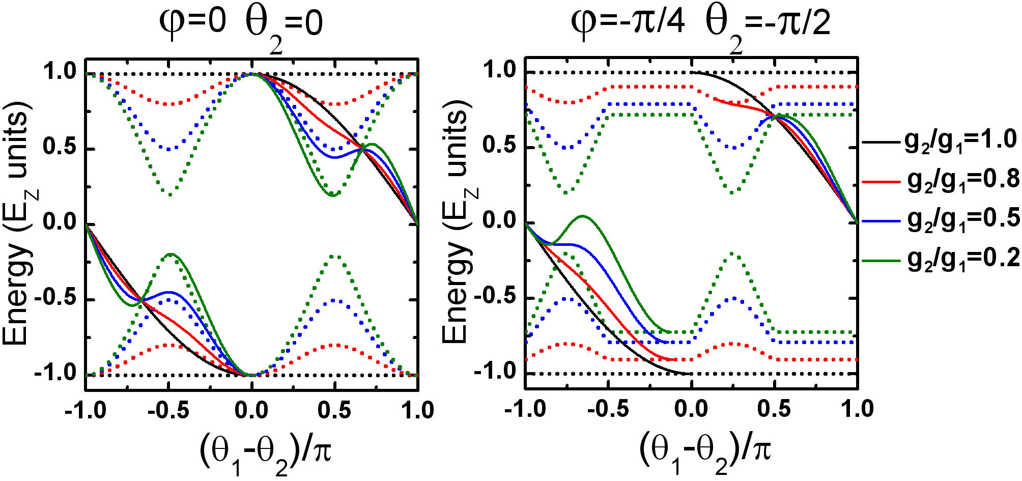
Figure 3: Energy of corner states $E_{\mathrm{0D}}-\varepsilon_{0}$ (solid curves) for different orientations of the magnetic field and edges relative to the main crystallographic axes, calculated for various ratio of $g_{2}/g_{1}$. We remind that $\varepsilon_{0}=C-\eta{M}$. The dotted curves represented by $\pm\min\{M_{1},M_{2}\}$ correspond to the boundaries of 1D edge band states projected onto the corner. The corner state arises as soon as $W(-\infty)W(+\infty)<0$. Note that $\theta_{1}-\theta_{2}\neq 0$ and $\pm\pi$ for physically reasonable edges forming a common corner.

Figure 3 shows the evolution of corner state energy as a function of $\theta_{1}-\theta_{2}$ at various ratio of $g_{2}/g_{1}$, calculated for several orientations of the magnetic field and edges. As seen, the corner state always appears from the gapped 1D edge bands. Each time the corner state merges with 1D edge, $W(-\infty)W(+\infty)$ causes to zero resulting to delocalization of the corner state (see Eq. (20). The boundaries of the 1D edge continuum projected onto the corner are determined by $\pm\min\{M_{1},M_{2}\}$ shown by dotted curves. Since both $H_{\mathrm{2D}}$ in Eq. (1) and $H_{Z}$ in Eq. (2) do not have electron-hole symmetry, the corner state energy $E_{\mathrm{0D}}$ depends on the orientation of the edges and the the magnetic field. Interestly, at specific values of $g_{2}/g_{1}$, $\theta_{1}$, $\theta_{2}$ and $\varphi$, the corner state may have a “zero energy” (which is $E_{\mathrm{0D}}=C$ in our notations) coinciding with the corner state energy in the system with particle-hole symmetry. However, this is the result of an arbitrary coincidence for a specific set of parameters , which are in no way related to any particular geometry of the edge and magnetic field orientations (except the case of $g_{e}^{||}=g_{h}^{||}$ and $\mathbb{D}=0$ SM ).

Our general analytical results represented by Eqs. (Magnetic-field-induced corner states in quantum spin Hall insulators)–(21) can also be applied for other QSHIs, for which the edge g-factor tensor is different from the one in Eq. (Magnetic-field-induced corner states in quantum spin Hall insulators). For instance, the edge g-factor tensor can be derived from the lowest-order in-$\mathbf{k}$ expansion of tight-binding Hamiltonians widely used to describe QSHIs within the lattice models Ezawa (2018c); Ren et al. (2020); Chen et al. (2020). As can be seen from Supplementary Materials SM , the analytical results obtained on the basis of Eq. (21) with the corresponding edge g-factor tensor perfectly reproduce the results of numerical calculations performed on the square lattice Ezawa (2018c).

Out-of-plane magnetic field.– Let us briefly discuss the effect of a perpendicular magnetic field $B_{z}$ in zinc-blende semiconductor QWs. The presence of BIA or IIA leads to the band-gap opening of the edge states even for the small values of $B_{z}$ Durnev and Tarasenko (2016). In this case, the terms describing the band-gap opening are written as

$$H_{\mathrm{edge}\bot}^{(\mathbf{B})}=\dfrac{\mu_{B}B_{z}}{2}\left(g_{xz}{s}_{x}+g_{yz}{s}_{y}\right),$$ (27)

where $g_{xz}$ and $g_{yz}$ have the following form:

$$g_{xz}=g_{3}\sin\theta,~{}~{}~{}~{}~{}~{}g_{yz}=-g_{3}\cos\theta.$$ (28)

Here, $g_{3}\sim\Omega^{3}\Delta$ is a non-zero constant Durnev and Tarasenko (2016) due to the presence of BIA or SIA in the zinc-blende QWs. Note that the diagonal component of the edge g-factor $g_{zz}$ is independent of $\theta$ and, thus, it can be formally nullified using the substitution $\hat{k}_{x}\rightarrow\hat{k}_{x}-g_{zz}\mu_{B}B_{z}/(2{\hbar}v_{F})$.

As clear, the form of $H_{\mathrm{edge}\bot}^{(\mathbf{B})}$ in Eq. (27) coincides with those for Hamiltonian (9). This means that out-of-plane magnetic field also leads to the corner state arising at the intersection of two meeting edges. Indeed, using the previously obtained results, the existence condition and energy of the corner state are directly written as

$$W(-\infty)W(+\infty)=-\dfrac{\mu_{B}^{2}g_{3}^{2}B_{z}^{2}}{4}\sin^{2}\left(\dfrac{\theta_{1}-\theta_{2}}{2}\right)<0,$$

$$E_{\mathrm{0D}\bot}=C-\eta{M}-\sigma\dfrac{\left|\mu_{B}g_{3}B_{z}\right|}{2}\cos\left(\dfrac{\theta_{1}-\theta_{2}}{2}\right).~{}~{}~{}~{}$$ (29)

As clear from Eq. (Magnetic-field-induced corner states in quantum spin Hall insulators), in the presence of BIA or IIA when $g_{3}\neq{0}$, the corner state induced by out-of-plane magnetic field exists for any crystallographic orientations of the meeting edges.

Corner states in the context of bulk band topology.– Finally, we summarize the conditions that dictate the protection of emerging corner states by the crystal symmetry in a 2D system. As discussed in details in Supplementary Materials SM , (001)-grown zinc-blende semiconductor QWs possess two highly symmetrical lines parallel to [$110$] and [$\bar{1}10$] crystallographic direction. When the magnetic field is oriented perpendicular to the one of the highly symmetrical lines, the 2D Hamiltonian is characterized by non-zero mirror-graded winding numbers, which formally indicate a HOTI state Bercioux et al. (2018).

From this perspective, the corners in zinc-blende QWs, whose 0D states are protected by mirror-reflection symmetry, are expected to be formed by the meeting edges that are mirror-symmetric with respect to the ($110$) and ($\bar{1}10$) planes, while magnetic field should be oriented perpendicular to the given mirror-symmetric plane SM . This includes both cases of in-plane and out-of plane magnetic field. Hence, the 0D states observed under the mentioned conditions could formally be classified as the states protected by crystal symmetry.

However, our analytical results reveal the presence of corner states over a much larger range of the meeting edges, including those that do not preserve the mirror-reflection symmetry. Obviously, the 0D states in the latter case are not associated with any symmetries and, therefore, they can not be classified as topological. Similar results are also obtained for QSHI lattice models that intentionally incorporate a broken electron-hole symmetry SM . Contrary to previous assumptions, our findings reveal that QSHIs, when subjected to a magnetic field, cannot be universally categorized as HOTIs, even though they exhibit non-zero mirror-graded winding numbers.

Nevertheless, as found previously in numerical simulations Ren et al. (2020), the presence of an electron-hole symmetry in the system stabilizes all corner states and make them robust, for instance, with respect to electrostatic disorder. The fact that electron-hole symmetry alone turns out to be sufficient for the stabilization of corner states was also recently established for hyperbolic lattices without translational symmetry Liu et al. (2023). However, even when considering the presence of electron-hole symmetry, the emergence of corner states in QSHIs is not inherently tied to the spatial symmetry of the system.

Summary.– We have analytically solved the general problem of magnetic-field-induced corner states in QSHIs without an electron-hole symmetry. The analysis performed within the continuous BHZ model reveals that the gapped edge states are described by the “generalized” 1D Dirac equation with two mass parameters, which nevertheless has a localized state at the intersection of two adjacent edges. Our study, focusing on QSHIs based on zinc-blende QWs, reveals the existence of localized states induced by an in-plane magnetic field at the corners. Remarkably, these states persist even in scenarios where the local preservation of crystal symmetry is absent. This means that the corner states in the latter case are not topological, and QSHI in the presence of a magnetic field cannot be considered as HOTI. Importantly, due to the absence of an inversion center, the corner states in zinc-blende semiconductor QWs can be also induced by a perpendicular magnetic field. Our analytical results, being applied to the QSHIs treated within the lattice models Ezawa (2018c); Ren et al. (2020); Chen et al. (2020), perfectly reproduce and extend understanding of the results previously obtained by numerical calculations Ezawa (2018c).

Supplementary Materials

.1 A. Uniqueness of the corner state energy for a sharp corner

As shown in the main text, the problem of finding the energy of a corner state localized at the intersection of two edges reduces to solving the equation

$$\Bigg{\{}\hat{k}_{x}^{2}+{W}(x)^{2}+\sigma{W}(x)^{\prime}\Bigg{\}}\psi(x)=\varepsilon{\psi}(x),$$ (S1)

where ${W}(x<0)=W_{1}$ and ${W}({x}\geq 0)=W_{2}$. Let us now demonstrate that with this choice of ${W}(x)$, the equation has only one localized solution at $\varepsilon=0$ if $W_{1}W_{2}<0$.

First, we note that Eq. (S1) is the central equation in the supersymmetric (SUSY) formulation of quantum mechanics Witten (1981). This equation has several exact analytical solutions found for specific forms of superpotential $W(x)$ during last decades Gangopadhyaya et al. (World Scientific, Singapore, 2011). Particularly, the one of solvable SUSY cases is represented by the superpotential in the form of Rosen-Morse II model Cooper et al. (World Scientific, Singapore, 2002):

$${W}(x)=A\tanh\left(\dfrac{x}{L}\right)+\dfrac{B}{A},$$ (S2)

where $L$ is dimensional scale, $A$ and $B$ are real constants related by $|B|<A^{2}$. The latter guarantees ${W}(-\infty){W}(+\infty)<0$. As clear, if $L\rightarrow{0}$, $W(x)$ is reduced to the case considered in the main text with $W_{1,2}=\mp{A}+B/A$. For ${W}(x)$ in the form of Eq. (S2), Eq. (S1) has localized solutions with the energies

$$\varepsilon(n_{\sigma})=A^{2}-\left(A-\dfrac{n_{\sigma}}{L}\right)^{2}+\dfrac{B^{2}}{A^{2}}-\dfrac{B^{2}}{\left(A-\dfrac{n_{\sigma}}{L}\right)^{2}},$$ (S3)

where $n_{-}/L=0,1,2,...,n_{max}/L<|A|$ for $\sigma=-1$ and $n_{+}/L=1,2,...,n_{max}/L<|A|$ for $\sigma=1$. Obviously, if $L\rightarrow{0}$, only a zero-energy solution with $n_{-}=0$ survives. The latter case corresponds to form of ${W}(x)$ considered in the main text.

.2 B. Corner states and Zeeman edge Hamiltonian from a lattice model used in Ref. Ezawa (2018)

The analytical theory of the appearance of corner states, developed in the main text, requires knowledge of the edge g-factor tensor, which in turn reflects the crystal symmetry of 2D system. In this section, we emphasize the difference between the edge Hamiltionians and thus the corner states arising in zinc-blende semiconductor QWs and the ones within a lattice model Ezawa (2018). Let us first derive the low-energy edge Hamiltonian obtained through the lowest-order expansion with respect to $\mathbf{k}$ of 2D bulk Hamiltonian used for the quantum spin Hall insulator (QSHI) on a square lattice. The wave-vector expansion of the lattice Hamiltonian used in Ref. Ezawa (2018) leads to the Hamiltonian similar to $H_{\mathrm{2D}}(\mathbf{k})$ in the main text:

$${H_{\mathrm{2D}}}^{\prime}(\mathbf{k})=C-\mathbb{D}k^{2}+\left(\mathbb{M}-\mathbb{B}k^{2}\right)\begin{pmatrix}\sigma_{z}&0\\ 0&\sigma_{z}\end{pmatrix}+A\begin{pmatrix}0&(k_{x}-{i}k_{y})\sigma_{x}\\ (k_{x}+{i}k_{y})\sigma_{x}&0\end{pmatrix},$$ (S4)

where we have added an additional term $-\mathbb{D}k^{2}$ describing the asymmetry between the conduction and valence bands, which is absent in the original paper Ezawa (2018). Other parameters in terms of the notations used in Ref. Ezawa (2018) are written as $M=m-2t$, $\mathbb{D}^{2}=-t|\mathbf{d}_{n}|$, $A=2\lambda|\mathbf{d}_{n}|$. The Zeeman Hamiltonian describing the effect of in-plane magnetic field has the form Ezawa (2018):

$${H_{\mathrm{Z}}}^{\prime}=\dfrac{\mu_{B}g_{0}}{2}\begin{pmatrix}0&0&B_{-}&0\\ 0&0&0&B_{-}\\ B_{+}&0&0&0\\ 0&B_{+}&0&0\end{pmatrix},$$ (S5)

where $B_{\pm}=B_{x}{\pm}iB_{y}$ and $g_{0}$ is a constant representing the in-plane g-factor. Here, $x$ and $y$ axes are oriented along the main crystallographic axes of the square lattice. Importantly, ${H_{\mathrm{Z}}}^{\prime}$ preserve the electron-hole symmetry.

In order to consider the edge of an arbitrary orientation, ${H_{\mathrm{2D}}}^{\prime}(\mathbf{k})$ and ${H_{\mathrm{Z}}}^{\prime}$ should be rewritten in a new coordinate system obtained by rotating clockwise along the $z$ axis by an angle $\theta$ relative to the original one (see Fig. 1 in the main text). To write the Hamiltonians in another coordinate system, one should transform the projections of electron momentum and magnetic field as:

$$\begin{pmatrix}k_{x}\\ k_{y}\end{pmatrix}=\begin{pmatrix}\cos{\theta}&-\sin{\theta}\\ \sin{\theta}&\cos{\theta}\end{pmatrix}\begin{pmatrix}\tilde{k}_{x}\\ \tilde{k}_{y}\end{pmatrix},~{}~{}~{}~{}~{}~{}~{}~{}~{}~{}~{}~{}~{}~{}~{}~{}\begin{pmatrix}B_{x}\\ B_{y}\end{pmatrix}=\begin{pmatrix}\cos{\theta}&-\sin{\theta}\\ \sin{\theta}&\cos{\theta}\end{pmatrix}\begin{pmatrix}\tilde{B}_{x}\\ \tilde{B}_{y}\end{pmatrix},$$ (S6)

where “tilde” denotes projections in the new coordinate system. Simultaneously with the transitions $\left(\tilde{k}_{x},\tilde{k}_{y}\right)\rightarrow\left(k_{x},k_{y}\right)$ and $\left(\tilde{B}_{x},\tilde{B}_{y}\right)\rightarrow\left(B_{x},B_{y}\right)$, one should also apply a unitary transformation to the Hamiltonians:

$${H_{\mathrm{2D}}}^{\prime}(\tilde{k}_{x},\tilde{k}_{y},\theta)=U^{\prime}(\theta){H_{\mathrm{2D}}}^{\prime}(k_{x},k_{y})U^{\prime}(-\theta),~{}~{}~{}~{}~{}~{}~{}~{}~{}~{}~{}~{}~{}~{}~{}~{}{H_{\mathrm{Z}}}^{\prime}(\tilde{B}_{x},\tilde{B}_{y},\theta)=U^{\prime}(\theta){H_{\mathrm{Z}}}^{\prime}(B_{x},B_{y})U^{\prime}(-\theta),$$ (S7)

where

$$U(\theta)=\begin{pmatrix}e^{i\theta/2}&0&0&0\\ 0&e^{i\theta/2}&0&0\\ 0&0&e^{-i\theta/2}&0\\ 0&0&0&e^{-i\theta/2}\end{pmatrix}.$$ (S8)

In contrast to the case of zinc-blende QWs considered in the main text, both ${H_{\mathrm{2D}}}^{\prime}(\tilde{\mathbf{k}})$ in Eq. (S4) and ${H_{\mathrm{Z}}}^{\prime}(\tilde{\mathbf{B}})$ in Eq. (S5) remains invariant under the coordinate system rotation. Further, we omit the tilde marks keeping in mind that orientation of new $x$ and $y$ axis does not coincide with the crystallographic directions in the most general case.

Then, assuming the open-boundary conditions in a semi-infinite plane $y>0$, the edge wave functions for at zero-wave vector along the boundary are written in the form:

$$|+\rangle=\dfrac{1}{\sqrt{2|\mathbb{B}|}}\begin{pmatrix}0\\ \sqrt{\mathbb{B}+\mathbb{D}}\\ \sqrt{\mathbb{B}-\mathbb{D}}\\ 0\end{pmatrix}g(y),~{}~{}~{}~{}~{}~{}~{}|-\rangle=\dfrac{1}{\sqrt{2|\mathbb{B}|}}\begin{pmatrix}-\sqrt{\mathbb{B}-\mathbb{D}}\\ 0\\ 0\\ \sqrt{\mathbb{B}+\mathbb{D}}\end{pmatrix}g(y)$$ (S9)

where $g(y)$ is a coordinate part of the wave-function describing the localization perpendicular to the edge.

By projecting the Zeeman Hamiltonian (S5) onto the obtained basis wave functions in Eq. (S9), one can verify that the edge g-factor tensor (see Eq. (6) in the main text) is independent of $\theta$ and has the following non-zero components:

$$g_{xx}^{\prime}=g_{0}\dfrac{\mathbb{D}}{\mathbb{B}},~{}~{}~{}~{}~{}~{}~{}g_{yy}^{\prime}=g_{0}.$$ (S10)

Finally, assuming the magnetic field is oriented as shown in Fig. 1 in the main text, the low-energy edge Hamiltonian is written as

$$H^{\prime}_{\mathrm{edge}}(k_{x})=\varepsilon_{0}+A\dfrac{\sqrt{\mathbb{B}^{2}-\mathbb{D}^{2}}}{\left|\mathbb{B}\right|}k_{x}{s}_{z}+M^{\prime}_{x}{s}_{x}+M^{\prime}_{y}{s}_{y},$$ (S11)

where $\varepsilon_{0}=C-\mathbb{M}\mathbb{D}/\mathbb{B}$, and

$$M^{\prime}_{x}=\dfrac{E^{\prime}_{Z}}{2}\eta\cos(\theta-\varphi),~{}~{}~{}~{}~{}~{}~{}M^{\prime}_{y}=\dfrac{E^{\prime}_{Z}}{2}\sin(\theta-\varphi)$$ (S12)

with $E^{\prime}_{Z}=\mu_{B}{B}g_{0}/2$ and $\eta=\mathbb{D}/\mathbb{B}$. As seen from Eq. (S12), at $\eta=0$, the edge states are gapless if the magnetic field is parallel to the edge of the 2D system. This reproduces the results of Ref. Ezawa (2018) obtained by numerical calculations of the local density of states within the square lattice model preserving electron-hole symmetry (see Fig. 2 therein). In the presence of electron-hole asymmetry, i.e. when $\eta\neq 0$, there are no gapless edge states, since the gap parameter $M^{\prime}$ for the edge states

$$M^{\prime}=\sqrt{{M^{\prime}}_{x}^{2}+{M^{\prime}}_{y}^{2}}=\sqrt{1-\left(1-\eta^{2}\right)\cos^{2}\left(\theta-\varphi\right)}\geq\left|\eta\right|$$ (S13)

never vanishes.

Let us now apply our general analytical results on the corner states to the edge Hamiltonian $H^{\prime}_{\mathrm{edge}}$ in Eqs. (S11) and (S12). In this case, Eq. (21) from the main text and the corner state existence condition are taking the form:

$$E_{\mathrm{0D}}=C-\eta\mathbb{M}+{E^{\prime}_{Z}}\dfrac{\sigma\eta\cos\left(\dfrac{\theta_{1}-\theta_{2}}{2}\right)}{\sqrt{\cos^{2}\left(\varphi-\dfrac{\theta_{1}+\theta_{2}}{2}\right)+\eta^{2}\sin^{2}\left(\varphi-\dfrac{\theta_{1}+\theta_{2}}{2}\right)}},~{}~{}~{}~{}~{}~{}~{}~{}~{}~{}~{}~{}~{}~{}~{}~{}~{}~{}~{}~{}~{}~{}~{}~{}~{}$$

$$W(-\infty)W(+\infty)={E^{\prime}_{Z}}^{2}\dfrac{\sin\left(\theta_{1}-\varphi\right)\cos\left(\varphi-\dfrac{\theta_{1}+\theta_{2}}{2}\right)+\eta^{2}\cos\left(\theta_{1}-\varphi\right)\sin\left(\varphi-\dfrac{\theta_{1}+\theta_{2}}{2}\right)}{\cos^{2}\left(\varphi-\dfrac{\theta_{1}+\theta_{2}}{2}\right)+\eta^{2}\sin^{2}\left(\varphi-\dfrac{\theta_{1}+\theta_{2}}{2}\right)}~{}~{}~{}~{}~{}~{}~{}~{}~{}~{}$$

$$\times\left[\sin\left(\theta_{2}-\varphi\right)\cos\left(\varphi-\dfrac{\theta_{1}+\theta_{2}}{2}\right)+\eta^{2}\cos\left(\theta_{2}-\varphi\right)\sin\left(\varphi-\dfrac{\theta_{1}+\theta_{2}}{2}\right)\right]<0.$$ (S14)

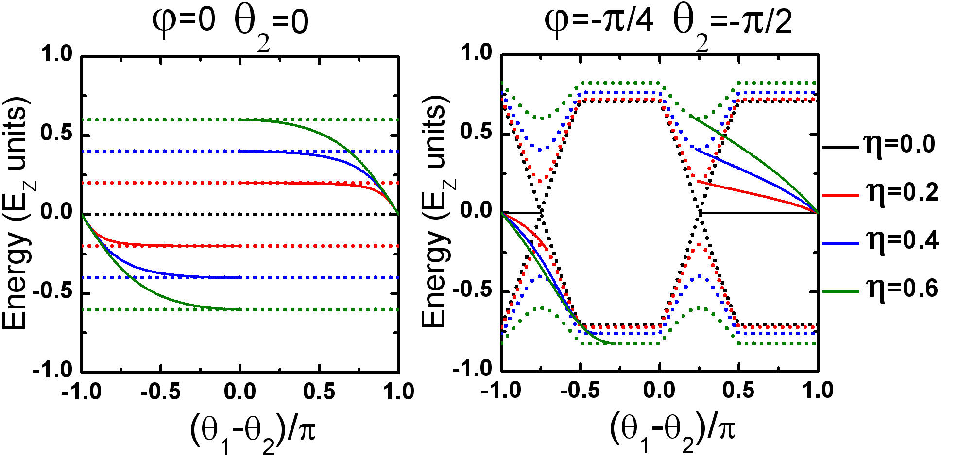
Figure S1: Energy of corner states $E_{\mathrm{0D}}-\varepsilon_{0}$ (solid curves) for different orientations of the magnetic field and edges relative to the main cubic axes, calculated at different values of $\eta$. The dotted curves represented by $\pm\min\{M_{1},M_{2}\}$ correspond to the boundaries of 1D edge band states projected onto the corner. The corner state arises as soon as $W(-\infty)W(+\infty)<0$. Note that $\theta_{1}-\theta_{2}\neq 0$ and $\pm\pi$ for physically reasonable edges forming a common corner.

Figure S1 shows the evolution of corner state energy as a function of $\theta_{1}-\theta_{2}$ at different values of $\eta$, calculated for several orientations of the magnetic field and edges (cf. Fig. 3 from the main text). If the magnetic field is oriented along the edge of 2D system (see the left panel at Fig. S1), a corner state exists only if the asymmetry parameter $\eta$ is nonzero. Otherwise (if $\eta=0$), the edge of 2D system parallel to the magnetic field has a gapless 1D edge spectrum, and there is no localized state in the corner. If the magnetic field is not parallel to each of the two edges, the corner state may appear even at $\eta=0$. Here, we would like to emphasize once again that the difference between Fig. S1 and Fig. 3 from the manin text is due to the difference in the QSHI and Zeeman Hamiltonians used in the lattice model Ezawa (2018) and for zinc-blende semiconductor QWs.

Expressions (.2) take very simple form if 2D system preserves electron-hole symmetry ($\eta$=0):

$$E_{\mathrm{0D}}=C,~{}~{}~{}~{}~{}~{}~{}~{}~{}~{}~{}~{}~{}~{}~{}~{}~{}~{}~{}~{}~{}~{}~{}~{}~{}~{}~{}~{}~{}$$

$$W(-\infty)W(+\infty)={E^{\prime}_{Z}}^{2}\sin\left(\theta_{1}-\varphi\right)\sin\left(\theta_{2}-\varphi\right)<0.$$ (S15)

As expected, the corner state energy $E_{\mathrm{0D}}=C$, which can be set to zero without loss of generality. It is also seen that if the magnetic field is oriented along one of the meeting edges, there is indeed no corner state since $W(-\infty)W(+\infty)=0$.

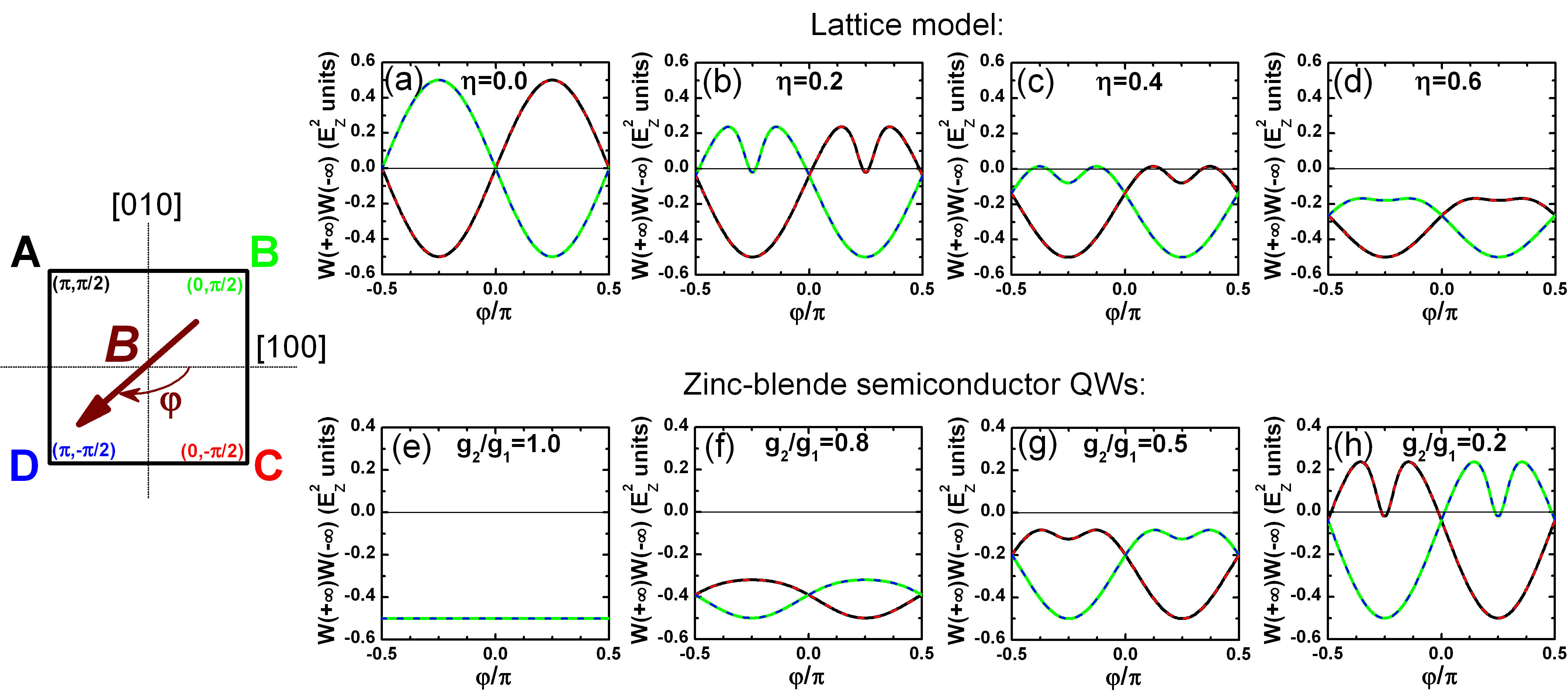
Figure S2: The corner states of a hypothetical sample with the edges along main crystallographic directions as a function of the magnetic field orientation. The numbers near the corners correspond to the values $\left(\theta_{1},\theta_{2}\right)$ that determine the orientations of the meeting edges in the notation used in this work. The direction of the magnetic field is determined by angle $\varphi$ as indicated by a brown arrow at the scheme. The positive values of the angles correspond to a clockwise rotation around $z$ axis. The localized state arises at each corner as soon as $W(-\infty)W(+\infty)<0$. The curves’ colors at the panels are related with the color corners at the scheme. The calculations on the basis on the 1D edge Hamiltonian derived from the lattice model Ezawa (2018) with additional electron-hole asymmetry are presented in panels (a)–(d).

For a more detailed comparison of our analytical results represented by Eqs. (.2) with numerical calculations in the lattice model with $\eta=0$ Ezawa (2018), we consider a hypothetical sample, whose edges are oriented along the main cubic axes (see Fig. S2). Note, however, that in our notations, the directions of the magnetic field considered in Ref. Ezawa (2018) correspond to $\varphi\in[-\pi/2,0]$ (cf. Fig. 2 in Ref. Ezawa (2018)). As seen from Fig. S2(a), the corners A, C always have a localized state if the magnetic field is oriented in the range of $\varphi\in(-\pi/2,0)$, while the corners B and D are stateless. This fully reproduces the results of numerical calculations presented in Fig. 2(b1)–(f1) in Ref. Ezawa (2018).

If there is an electron-hole asymmetry in 2D system (i.e. $\eta\neq{0}$) – this case was not considered in Ref. Ezawa (2018) – the appearance of localized states in all four corners becomes possible. At first, such situation arises at small values of $\eta$ for the directions of the magnetic field $\varphi=\pm\pi/4$, $\pm 3\pi/4$. Note, however, that if $\varphi=-\pi/4$, $3\pi/4$, the states in the corners B and D are localized on a much larger scale than the states at the corners A and C. The localization scale is qualitatively determined by the quantity $W(-\infty)W(+\infty)$. As the parameter $\eta$ increases, the four corner states at once are possible for wider angle $\varphi$ intervals, until eventually the presence of the states localized in the corners A, B, C and D ceases to depend on the direction of the magnetic field when $\eta$ exceeds some critical value $\eta_{c}$.

For comparison, Fig. S2 also shows $W(-\infty)W(+\infty)$ at all four corners calculated for zinc-blende semiconductor QWs at different ratio of $g_{2}/g_{1}$ (see the main text for its definitions).

.3 C. Nontrivial bulk band topology

In the main text and previous section, we have found the energies of 0D state localized at the intersection of two meeting edges, which exists in a wide range of the orientations of the edges and magnetic field. On the other hand, the appearance of such corner states is often related to higher-order topological insulator (HOTI) state, arising due to the crystal symmetry. Indeed, although the presence of the Zeeman field breaks the time-reversal symmetry and thus destroys QSHI state, an in-plane Zeeman field preserves various crystalline symmetries of the system (such as inversion, mirror-reflection, rotation or even particle-hole symmetry), making it possible to exhibit various topological crystalline phases. Below, we discuss the symmetry prerequisites for arising of the corner states in various QSHIs.

.3.1 QSHI with the model considered in Section B

Let us first consider an example of QSHI described by axially symmetric Hamiltonian ${H_{\mathrm{2D}}}^{\prime}(k_{x},k_{y})$ in Eq. (S4). Without loss of generality, we assume that the in-plane magnetic field is oriented along the $y$ axis. In this case, ${H_{\mathrm{2D}}}^{\prime}(k_{x},0)+{H_{\mathrm{Z}}}^{\prime}$ is invariant under mirror-reflection symmetry operation $\mathcal{M}_{y}$ that changes $y$ to $-y$:

$$\mathcal{M}_{y}=\begin{pmatrix}0&\sigma_{z}\\ -\sigma_{z}&0\end{pmatrix}$$ (S16)

By applying $\mathcal{M}_{y}$ twice, one can get $\mathcal{M}_{y}^{2}=-1$, meaning that $\mathcal{M}_{y}$ has two eigenvalues of $\pm{i}$. A unitary transformation consisting of the eigenvectors of the operator $\mathcal{M}_{y}$

$$\mathcal{U}^{\prime}=\dfrac{1}{2}\begin{pmatrix}1&1&-i&-i\\ -1&1&-i&i\\ -i&-i&1&1\\ -i&i&-1&1\end{pmatrix}$$ (S17)

reduces the Hamiltonian ${H_{\mathrm{2D}}}^{\prime}(k_{x},0)+{H_{\mathrm{Z}}}^{\prime}$ to the block-diagonal form

$${\mathcal{U}^{\prime}}^{{\dagger}}\left\{{H_{\mathrm{2D}}}^{\prime}(k_{x},0)+{H_{\mathrm{Z}}}^{\prime}\right\}{\mathcal{U}^{\prime}}=C+\begin{pmatrix}h^{\prime}_{0}+{h^{\prime}}_{x}^{(-)}\sigma_{x}+{h^{\prime}}_{y}^{(-)}\sigma_{y}&0\\ 0&h^{\prime}_{0}+{h^{\prime}}_{x}^{(+)}\sigma_{x}+{h^{\prime}}_{y}^{(+)}\sigma_{y}\end{pmatrix},$$ (S18)

where the upper and lower blocks correspond to $-i$ and $i$ eigenvalues of $\mathcal{M}_{y}$, respectively. Here,

$$h^{\prime}_{0}=-\mathbb{D}k_{x}^{2},~{}~{}~{}~{}~{}~{}~{}~{}~{}{h^{\prime}}_{x}^{(\pm)}=\mathbb{M}\pm\dfrac{\mu_{B}g_{0}{B_{y}}}{2}-\mathbb{B}k^{2}_{x},~{}~{}~{}~{}~{}~{}~{}~{}~{}{h^{\prime}}_{y}^{(\pm)}=-A{k_{x}}.$$ (S19)

Each of the blocks in Eq. (S18) is characterized by mirror-graded winding number (also known as Zak phase), that can be calculated by

$$\nu=\dfrac{1}{2\pi}\int\limits_{-\infty}^{+\infty}d{k_{x}}\dfrac{{h^{\prime}}_{x}\partial_{k_{x}}{{h^{\prime}}_{y}}-{h^{\prime}}_{y}\partial_{k}{{h^{\prime}}_{x}}}{{h^{\prime}}_{x}^{2}+{h^{\prime}}_{y}^{2}}.$$ (S20)

Note that Eq. (S20) is also valid at arbitrary values of $h^{\prime}_{0}$ (see Section D).

Substituting the ${h^{\prime}}_{x}$ and ${h^{\prime}}_{y}$ from Eq. (S19), straightforward calculations lead to the following result

$$\nu^{(\pm)}=-\dfrac{1}{2\pi}\left[\arctan\left\{\dfrac{\mathbb{B}}{A}k_{x}\right\}+\arctan\left\{\dfrac{\mathbb{B}^{2}}{A\left(\mathbb{M}\pm\dfrac{\mu_{B}g_{0}{B_{y}}}{2}\right)}k_{x}^{3}+\left(\dfrac{A}{\mathbb{M}\pm\dfrac{\mu_{B}g_{0}{B_{y}}}{2}}-\dfrac{\mathbb{B}}{A}\right)k_{x}\right\}\right]\Bigg{|}_{-\infty}^{+\infty}.$$ (S21)

We note that the existence condition of QSHI state in the absence of magnetic field requires that $\mathbb{Z}_{2}$ invariant

$$\nu_{\mathbb{Z}_{2}}=-\dfrac{1}{2}\left\{\mathrm{sgn}(\mathbb{M})+\mathrm{sgn}(\mathbb{B})\right\}=1,$$ (S22)

which is fulfilled if $\mathbb{B}$ and $\mathbb{M}$ are both negative Bernevig et al. (2006); Liu et al. (2008). The latter reduces Eq. (S21) at small values of $B_{y}$ to $\nu^{(\pm)}=\mathrm{sgn}(A)$, which is equal $1$ or $-1$ depending on the sign of $A$. This non-zero mirror-graded winding number indicates the system a HOTI with in-gap corner states Bercioux et al. (Springer Nature, Switzerland AG, 2018); Ren et al. (2020).

Since the Hamiltonian ${H_{\mathrm{2D}}}^{\prime}(k_{x},k_{y})+{H_{\mathrm{Z}}}^{\prime}$ is axially symmetric, then any direction perpendicular to the magnetic field will be highly symmetrical, characterized by the non-trivial winding numbers. From this perspective, the corners that are mirror-symmetric with respect to such highly symmetrical line should have topologically stable corner states, which cannot be continuously removed from the gap by the perturbation preserving such mirror reflection symmetry. For the corners shown in Fig. S2, the magnetic field orientation, at which the corner states are protected by mirror symmetry, corresponds to $\varphi=\pm\pi/4$ and $\pm 3\pi/4$. The corner states arising at other magnetic field orientations are, strictly speaking, not topologically stable.

At $\mathbb{D}=0$, the 2D system has an additional electron-hole symmetry, which is preserved even in the presence of in-plane magnetic field due to the form of the Zeeman energy in Eq. (S5). The presence of electron-hole symmetry significantly expands the range of parameters for topological corner states that are protected by this particular symmetry. In this case, considered in Ref. Ezawa (2018); Ren et al. (2020), the corner state, if it exists, it has only the “zero energy” $E_{\mathrm{0D}}=C$ as clear from Eq. (.2). Moreover, the presence of any electrostatic disorder (which breaks the mirror-reflection symmetry in the system but preserves the electron-hole one) is not sufficient to shift the corner state energy from $E_{\mathrm{0D}}=C$ and thus to remove it from the gap. As clear from Eq. (S11), one of the mass terms for 1D states vanishes in this case, and the corner states are uniquely identified as the Jackiw-Rebbi topological domain wall modes Jackiw and Rebbi (1976). The fact that the presence of electron-hole symmetry alone turns out to be sufficient for the stabilization of corner states was recently established for hyperbolic lattices without translational symmetry Liu et al. (2023). In this sense, the corner states that appear in Fig. S2 at $\mathbb{D}=0$ (i.e. $\eta=0$) for any orientations of the magnetic field are topological.

.3.2 QSHIs based on zinc-blende semiconductors

In contrast to the case considered above, the low-energy Hamiltonian of QSHIs based zinc-blende semiconductors is not axially symmetric. However, it preserves mirror-reflection symmetry along some crystallographic directions, which also makes it possible to characterize the bulk states by means of mirror-graded winding numbers, as will be shown below. Assuming the magnetic field is oriented in the same way as in Fig. 1 in the main text, a unitary transformation consisting of the eigenvectors of the operator $\mathcal{M}_{y}$ in Eq. (S16) is conveniently chosen in the form $\mathcal{U}=\mathcal{U}^{\prime}\mathcal{S}$, where

$$\mathcal{S}=\dfrac{1}{\sqrt{2}}\begin{pmatrix}1&-i&0&0\\ -i&1&0&0\\ 0&0&1&-i\\ 0&0&-i&1\end{pmatrix}.$$ (S23)

This transformation brings the Hamiltonian ${H_{\mathrm{2D}}}(k_{x},0)+{H_{\mathrm{Z}}}$ (see Eqs. (1) and (2) in the main text) to the form

$${\mathcal{U}}^{{\dagger}}\left\{{H_{\mathrm{2D}}}(k_{x},0)+{H_{\mathrm{Z}}}\right\}{\mathcal{U}}=C+\begin{pmatrix}h_{0}^{(-)}+h_{x}^{(-)}\sigma_{x}+h_{y}^{(-)}\sigma_{y}&0\\ 0&h_{0}^{(+)}+h_{x}^{(+)}\sigma_{x}+h_{y}^{(+)}\sigma_{y}\end{pmatrix}+\\ \Delta\cos{2\theta}\begin{pmatrix}0&0&i&0\\ 0&0&0&-i\\ -i&0&0&0\\ 0&i&0&0\end{pmatrix}+\dfrac{\mu_{B}{B_{y}}}{4}g_{e}^{||}\cos{(\theta-\varphi)}\begin{pmatrix}0&0&1&1\\ 0&0&1&1\\ 1&1&0&0\\ 1&1&0&0\end{pmatrix}+\dfrac{\mu_{B}{B_{y}}}{4}g_{h}^{||}\cos{(5\theta-\varphi)}\begin{pmatrix}0&0&1&-1\\ 0&0&-1&1\\ 1&-1&0&0\\ -1&1&0&0\end{pmatrix},$$ (S24)

where

$$h_{0}^{(\pm)}=\mp\dfrac{\mu_{B}{B_{y}}}{4}\left[g_{e}^{||}\sin{(\theta-\varphi)}+g_{h}^{||}\sin{(5\theta-\varphi)}\right]-\mathbb{D}k_{x}^{2},~{}$$

$$h_{x}^{(\pm)}=\mathbb{M}\mp\dfrac{\mu_{B}{B_{y}}}{4}\left[g_{e}^{||}\sin{(\theta-\varphi)}-g_{h}^{||}\sin{(5\theta-\varphi)}\right]-\mathbb{B}k^{2}_{x},~{}$$

$$h_{y}^{(\pm)}=\Delta\sin{2\theta}\pm{A{k_{x}}}.~{}~{}~{}~{}~{}~{}~{}~{}~{}~{}~{}~{}~{}~{}~{}$$ (S25)

As clear, Eq. (S24) reduces to a block-diagonal form, with the upper and lower blocks corresponding to $-i$ and $i$ eigenvalues of $\mathcal{M}_{y}$, respectively, if $\theta=\theta^{*}$ and $\varphi=\varphi^{*}$, where $\theta^{*}$ equals to $\pm{\pi}/4$ (or $\pm{3\pi}/4$) and $\varphi^{*}-\theta^{*}=\pm{\pi}/2$ (or $\pm{3\pi}/2$) for a non-zero $\Delta$. As it is seen from Fig 1 in the main text, at these $\theta^{*}$ values, the $k_{y}=0$ plane corresponds to the ($110$) and ($\bar{1}10$) planes. These crystallographic planes are mirror reflection planes for (001)-grown zinc-blende QWs with a $D_{2d}$ symmetry. Note that the magnetic field in this case is oriented perpendicular to the plane of $\theta=\theta^{*}$.

Thus, the highly symmetric lines formed by the intersection of the mirror reflection planes with the growth QW plane are invariant under $\mathcal{M}_{y}$. This allows representation of the Hamiltonian ${H_{\mathrm{2D}}}(k_{x},0)+{H_{\mathrm{Z}}}$ in a block-diagonal form, in which each block corresponds to the given eigenvalue of $\mathcal{M}_{y}$. Similar to the case considered previously, the Hamiltonian (S24) at $\theta=\theta^{*}$ and $\varphi=\varphi^{*}$ is characterized by mirror-graded winding numbers $\nu^{(\pm)}$ calculated in accordance with Eq. (S20) as

$$\nu^{(s)}=-\dfrac{1}{2\pi}\left[\arctan\left\{\dfrac{\mathbb{B}}{sA}k_{x}+\dfrac{\mathbb{B}\Delta\sin 2\theta^{*}}{A^{2}}\right\}+\arctan\left\{\dfrac{sA}{\mathbb{M}^{(s)}}\dfrac{\mathbb{B}^{2}}{A^{2}-\dfrac{\mathbb{B}}{\mathbb{M}^{(s)}}\Delta^{2}\sin^{2}2\theta^{*}}k_{x}^{3}+\mathcal{F}^{(s)}(k_{x})\right\}\right]\Bigg{|}_{-\infty}^{+\infty},$$ (S26)

where

$$\mathcal{F}^{(s)}(k_{x})=\dfrac{\mathbb{B}^{2}\Delta\sin 2\theta^{*}}{A^{2}\mathbb{M}^{(s)}-\mathbb{B}\Delta^{2}\sin^{2}{2\theta^{*}}}k_{x}^{2}+sA\dfrac{A^{2}-\mathbb{B}\mathbb{M}^{(s)}}{A^{2}\mathbb{M}^{(s)}-\mathbb{B}\Delta^{2}\sin^{2}{2\theta^{*}}}k_{x}-\Delta\sin 2\theta^{*}\dfrac{A^{2}+\mathbb{B}\mathbb{M}^{(s)}}{A^{2}\mathbb{M}^{(s)}-\mathbb{B}\Delta^{2}\sin^{2}{2\theta^{*}}},$$

$$\mathbb{M}^{(s)}=\mathbb{M}-s\dfrac{\mu_{B}{B_{y}}}{4}\left[g_{e}^{||}\sin{(\theta-\varphi)}-g_{h}^{||}\sin{(5\theta-\varphi)}\right].~{}~{}~{}~{}~{}~{}~{}~{}~{}~{}~{}~{}~{}~{}~{}~{}~{}~{}~{}~{}~{}~{}~{}~{}~{}~{}~{}~{}~{}~{}~{}~{}~{}$$

Then, assuming both $\mathbb{B}$ and $\mathbb{M}$ to be negative, which guarantees that $\nu_{\mathbb{Z}_{2}}=1$ in the absence of magnetic field (see Eq. (S22)), straightforward calculations lead to $\nu^{(s)}=\mathrm{sgn}(sA)$ at small values of $B_{y}$. Note that the magnetic field $B_{y}$ is assumed to be small in the sense that $\mathrm{sgn}(\mathbb{M})=\mathrm{sgn}(\mathbb{M}^{(s)})$. Thus, depending on the sign of $A$, the non-zero mirror-graded winding number $\nu^{(\pm)}$ is either $+1$ or $-1$, which indicates the system a HOTI with in-gap corner states Bercioux et al. (Springer Nature, Switzerland AG, 2018); Ren et al. (2020). Similarly, one can calculate the mirror-graded winding numbers for the case of out-of-plane magnetic field, briefly outlined in the main text.

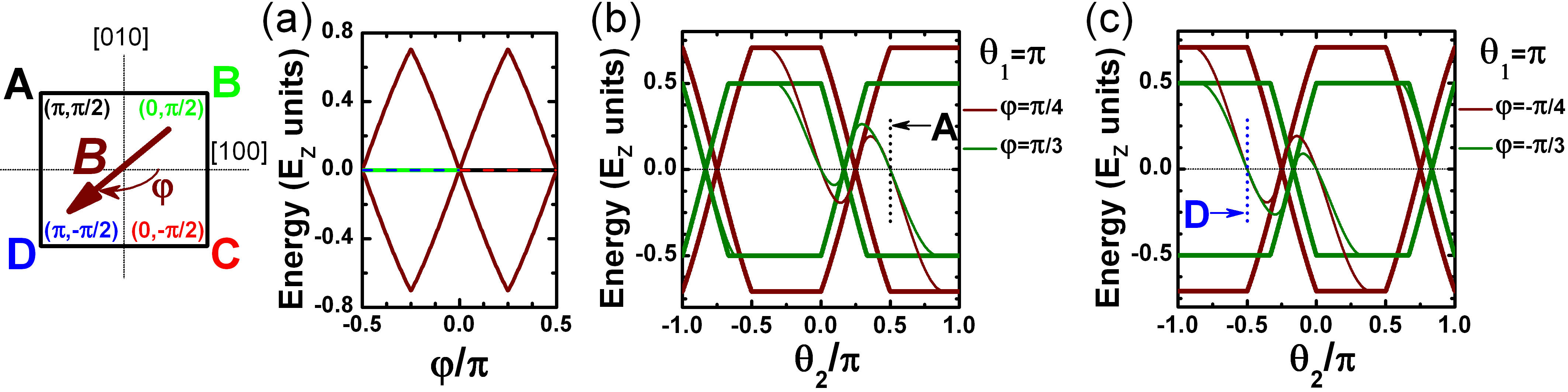
Figure S3: (a) “Zero-energy” corner states $E_{\mathrm{0D}}=C$ in zinc-blende QWs at $\mathbb{D}=0$ and $g_{e}^{||}=g_{h}^{||}$ (the chiral case) of a hypothetical sample with the edges along main crystallographic directions. The brown solid curves correspond to the boundaries of 1D edge band states projected onto the corners. (b,c) Energy of corner states $E_{\mathrm{0D}}-C$ (thin solid curves) for different orientations of the magnetic field and edges relative to the main cubic axes at $\theta_{1}=\pi$. The bold solid curves correspond to the boundaries of 1D edge band states projected onto the corner. The zero-energy corner states arise only for corners whose edges are mirror-symmetric with respect to the ($110$) and ($\bar{1}10$) planes. The values of $\theta_{2}$ corresponding to the angles “A” and “D” of the hypothetical sample are marked with dotted vertical lines. Other notations are the same as in Fig S2. Note that $\theta_{1}-\theta_{2}\neq 0$ and $\pm\pi$ for physically reasonable edges forming a common corner.

In contrast to the QSHI model considered in Ref. Ezawa (2018), the Hamiltonian of zinc-blende semiconductor QWs does not possess an electron-hole symmetry at $\mathbb{D}=0$. However, the transformed Hamiltonian ${H_{\mathrm{2D}}}(k_{x},0)+{H_{\mathrm{Z}}}$ in Eq. (S24) has additional chiral symmetry for along the ($110$) and ($\bar{1}10$) planes if $g_{e}^{||}=g_{h}^{||}$. The presence of such chiral symmetry results in the “zero-energy” corner states with $E_{\mathrm{0D}}={C}$ for the meeting edges that are mirror-symmetric with respect to the ($110$) and ($\bar{1}10$) planes. For other edges, the energy of corner states shifts away from the “zero energy” as displayed in Fig. S3. This is a representative example of the fact that although a chiral symmetry leads to the “zero-energy” corner states, it is primarily associated with mirror symmetry, which holds for only certain corners of zinc-blende QSHIs. Unfortunately, realistic QSHIs based on zinc-blende semiconductors, such as HgTe/CdHgTe QWs and InAs/GaInSb QW heterostructures do not possess the “zero-energy” states, since their existence conditions $\mathbb{D}=0$ and $g_{e}^{||}=g_{h}^{||}$ are fundamentally unattainable therein.

As clear from above, the corner states in zinc-blende QSHIs are protected by mirror-reflection symmetry only for corners that are mirror-symmetric with respect to the ($110$) and ($\bar{1}10$) planes, while the magnetic field should be oriented perpendicular to the given mirror-symmetric line of 2D system. The latter includes both cases of in-plane and out-of plane magnetic field.

.4 D. Winding number in 1D system

It is believed that Eq. (S20) is valid only if the 1D system has chiral symmetry, i.e., when $h_{0}=0$. In this section, we will show that it can also be applied in the absence of chiral symmetry with a non-zero $h_{0}$. Let us consider the most generic Hamiltonian for a two-band 1D system given by

$$H_{\mathrm{1D}}(k)=h_{0}(k)+h_{x}(k)\sigma_{x}+h_{y}(k)\sigma_{y}+h_{z}(k)\sigma_{z},$$ (S27)

which has two eigenvalues $E=h_{0}\pm\sqrt{h_{x}^{2}+h_{y}^{2}+h_{z}^{2}}$. The eigenvectors of $H_{\mathrm{1D}}$ in Eq. (S27) at given energy $E$ can be written as system given by

$$\Psi_{\mathrm{1D}}(k)=\dfrac{1}{\sqrt{2(E-h_{0})(E-h_{0}-h_{z})}}\begin{pmatrix}h_{x}-i{h_{y}}\\ E-h_{0}-h_{z}\end{pmatrix}.$$ (S28)

Knowing the wave functions, a winding number (Zak phase) is calculated in general form as

$$\nu=\dfrac{i}{2\pi}\int\limits_{-\infty}^{+\infty}d{k}\langle\Psi_{\mathrm{1D}}(k)|\partial_{k}|\Psi_{\mathrm{1D}}(k)\rangle.$$ (S29)

The calculation of $\nu$ is greatly simplified if $h_{z}(k)\equiv{0}$, while $h_{0}(k)$ is still an arbitrary function of $k$. In this case, Eq. (S28) is reduced to

$$\Psi_{\mathrm{1D}}(k)=\dfrac{1}{\sqrt{2}}\begin{pmatrix}\dfrac{h_{x}-i{h_{y}}}{\sqrt{h_{x}^{2}+h_{y}^{2}}}\\ \pm{1}\end{pmatrix},$$ (S30)

where “$+$” and “$-$” correspond to the conduction band and valence band, respectively. This allows rewriting Eq. (S29) in the form

$$\nu=\dfrac{1}{2\pi}\int\limits_{-\infty}^{+\infty}d{k}\dfrac{h_{x}\partial_{k}{h_{y}}-h_{y}\partial_{k}{h_{x}}}{h_{x}^{2}+h_{y}^{2}}.$$ (S31)

References

- Witten (1981) E. Witten, Nucl. Phys. B 188, 513 (1981).
- Gangopadhyaya et al. (World Scientific, Singapore, 2011) A. Gangopadhyaya, J. V. Mallow, and C. Rasinariu, Supersymmetric Quantum Mechanics: An Introduction (World Scientific, Singapore, 2011).
- Cooper et al. (World Scientific, Singapore, 2002) F. Cooper, A. Khare, and U. Sukhatme, Supersymmetry in Quantum Mechanics (World Scientific, Singapore, 2002).
- Ezawa (2018) M. Ezawa, Phys. Rev. Lett. 121, 116801 (2018).
- Bernevig et al. (2006) B. A. Bernevig, T. L. Hughes, and S.-C. Zhang, Science 314, 1757 (2006).
- Liu et al. (2008) C. Liu, T. L. Hughes, X.-L. Qi, K. Wang, and S.-C. Zhang, Phys. Rev. Lett. 100, 236601 (2008).
- Bercioux et al. (Springer Nature, Switzerland AG, 2018) D. Bercioux, J. Cayssol, M. G. Vergniory, and M. R. Calvo, Topological Matter: Lectures from the Topological Matter School 2017 (Springer Nature, Switzerland AG, 2018).
- Ren et al. (2020) Y. Ren, Z. Qiao, and Q. Niu, Phys. Rev. Lett. 124, 166804 (2020).
- Jackiw and Rebbi (1976) R. Jackiw and C. Rebbi, Phys. Rev. D 13, 3398 (1976), URL https://link.aps.org/doi/10.1103/PhysRevD.13.3398.
- Liu et al. (2023) Z.-R. Liu, C.-B. Hua, T. Peng, R. Chen, and B. Zhou, Phys. Rev. B 107, 125302 (2023), URL https://link.aps.org/doi/10.1103/PhysRevB.107.125302.