[a,b]A. Corstanje
Prospects for measuring the longitudinal particle distribution of cosmic-ray air showers with SKA
Abstract
We explore the possibilities of measuring the longitudinal profile of individual air showers beyond when using very dense radio arrays such as SKA. The low-frequency part of the Square Kilometre Array, to be built in Australia, features an enormous antenna density of about 50,000 antennas in the inner core region of radius 500 m, with a frequency band from 50 to 350 MHz. From CoREAS simulations, a SKA-Low antenna model plus noise contributions, and adapted LOFAR analysis scripts, we obtain a resolution in the shower maximum and energy that is considerably better than at LOFAR. Already from this setup, we show that at least one additional parameter of the longitudinal profile can be measured. This would improve mass composition analysis by measuring an additional composition-dependent quantity. Moreover, it would offer an opportunity to discriminate between the different predictions of hadronic interaction models, hence contributing to hadronic physics at energy levels beyond man-made accelerators.
1 Introduction
The low-frequency part of the Square Kilometre Array [1] to be built in Australia will feature an unprecedented number and density of antennas. Whereas LOFAR [2] has about 300 usable antennas in a diameter of , SKA will have about in a radius of , and extends the frequency band to . Hence, it is expected to open up new possibilities in measuring air showers into fine detail.
LOFAR has been successful in measuring to an accuracy suitable for cosmic-ray mass composition studies [3, 4]. The longitudinal evolution of the number of particles in an air shower, reaching a maximum at , has two extra parameters containing information about mass composition; moreover, their expected value and distribution varies with hadronic interaction model [5]. Hence, being able to measure these would offer an opportunity to improve mass composition measurements, and to distinguish between hadronic interaction models at high energies.
Here we report a first analysis to reconstruct longitudinal profile parameters.
2 Methods
The longitudinal particle distribution of air showers, of which an example is shown in Fig. 1, can be parametrized by three parameters , , and [6]. The distribution function is
| (1) |
with denoting the number of particles, and the traversed depth in the atmosphere in . In this distribution, is the maximum or mode, is related to the variance (second moment), and to the skewness (third moment). The effect of varying and is demonstrated in Fig. 1.


In radio measurements at LOFAR, we have focused on reconstructing , as this is the parameter to which the radio footprint is most sensitive. To investigate the possibilities of reconstructing and with SKA, we have simulated an ensemble of proton showers at an energy of , coming from east at a zenith angle of 30 degrees. Simulations were done with Corsika and CoREAS 7.7410 [7, 8] at a thinning level of . Using pre-selection of showers with CONEX [9], these showers were selected to have an (from Corsika) of , all within a range of . For this, simulating about 50000 Conex showers and 500 Corsika showers is sufficient for producing the showers with Corsika plus CoREAS. Having effectively taken out the -variations, we can focus on the effect of variations of and on the radio footprint.
The present analysis focuses on two parts: comparing radio footprints directly as a function of and , and doing a more complete reconstruction of , , and using simulated measurements with realistic sky noise.
2.1 Interpolation based on Fourier series
Our simulations have antennas put on a radial grid or ‘star shape’, with radial density higher in the first from the core, then declining outward. For a reconstruction from a dense layout of antennas, an interpolation is needed. We have developed an interpolation method that improves over the radial basis function method [10] used earlier, which does not perform as well on footprints of higher-frequency signals. It makes use of the natural radial structure of the footprint, and of the (mainly) -dependence of the pulse energy from geomagnetic and charge-excess origin combined.
On a radial grid, the energy along the angular direction (at constant radius) can be expressed as a Fourier series, by taking an FFT. In our case, the FFT is done on 8 points (simulated antennas) along a circle at each radius, and for convenience we express the result in cosine and sine amplitudes, here denoted by and for mode at radius . This is a complete representation of the values along a circle, provided it is sampled densely enough (the Nyquist criterion on spatial frequencies).
The interpolated footprint energy at position along a circle of radius is given by
| (2) |
For interpolation in the radial direction, a standard one-dimensional interpolation is used on the angular Fourier components and separately. A cubic spline interpolation was found useful here. After this, Eq. 2 can be used at any position within the radial boundaries of the simulated antennas. Using this method, simulations having on the order of antennas would suffice for producing pulse energy footprints to an accuracy as desired for application to SKA measurements. A dedicated publication on this method and its precision is forthcoming.
2.2 Direct comparison of equal- footprints as a function of and
A direct comparison between footprints is made by determining the mean squared error (MSE) when taking their difference on each simulated antenna position, fitting a constant scale factor. This amounts to
| (3) |
with the best-fit energy scale factor , and the pulse energies in shower . The MSE is the ‘noiseless’ equivalent of the used when fitting simulations to realistic data with noise.
A second way of comparing footprints is to consider the (lowest-order) Fourier amplitudes as a function of distance to shower core. Taking one shower as reference, e.g. around the median value of in the ensemble, we take the difference between showers of the angular-constant and modes, respectively.
2.3 Monte Carlo setup for simulated air shower reconstruction at SKA
To mimic the essential steps of the reconstruction process at SKA, we make use of the simulated ensemble of CoREAS showers to create mock data. The signals at each simulated antenna are passed through the SKALA2 antenna model [11], giving voltages as they would be seen at the AD converters. Realistic levels of (frequency-dependent) sky noise are added to the simulated pulse signal at each antenna on the radial grid. The power spectrum of sky noise is taken from LFMap [12] as was used for calibration of the LOFAR antennas [13]. We scale the simulated pulse amplitudes, to mimic an energy of , to increase the signal-to-noise ratio in a restricted band of 50 to .
The pulse energy is measured in a time window around the pulse maximum, with a width of for the full to bandwidth, or when restricting to to . A (non-tight) trigger criterion of above the noise is used to obtain a trigger probability versus pulse energy. By taking 300 noise realisations, we obtain an uncertainty on measured pulse energy at each antenna position. Now, we use the interpolation method from Sect. 2.1 to obtain pulse energy and its uncertainty at each SKA antenna position in the proposed layout.
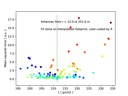
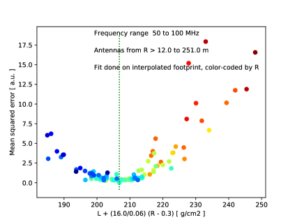
3 Results of direct comparison
We have taken a shower around the median value of in our ensemble, and computed the MSE when fitting each of the other showers to it. We have restricted the frequency range to to as the effects shown below appear most clearly in this lower frequency band. The result is shown in the left panel of Fig. 2, as a function of and color-coded by . It is seen that no clear minimum arises, but there appears to be a non-random variation with .
Therefore, we consider expressing the MSE as a function of a combination of and , obtaining the right panel of Fig. 2. The simplest combination is a linear function of and , with a constant coefficient to put them on the same dimension of . We introduce a sensitive parameter as
| (4) |
where the numbers and are approximately the half-range and the median value of , respectively. The coefficient value of depends on the frequency range, and possibly on other shower parameters such as and zenith angle which were kept constant here. This shows a clear minimum around the correct position, and (to lowest order) a parabolic shape around it, as familiar from reconstructions. We conclude that when comparing footprints in this way, they are sensitive to the parameter rather than to and individually. A way to interpret this is to consider the leading and trailing curves in Fig. 1, noting that the footprint must be sensitive to the region around , hence to a combination of the curve before and after . This combination may well be different from the definitions of and in Eq. 1, depending e.g. on the shower geometry.
3.1 Angular Fourier modes as function of distance to shower core
In Fig. 3 we look at the two leading Fourier modes, being the angular-constant and -mode. The median- shower is taken as baseline, and the difference of all other showers with respect to this shower is plotted, color-coded by the parameter described above. It is seen from the left panel that at low values of , the footprint has relatively more energy in the inner part, at a core distance below about . The right panel shows that additionally, the angular dependence is stronger for these showers as well in the inner part, both in the absolute sense as plotted here, and relative to the (dominant) angular-constant mode.
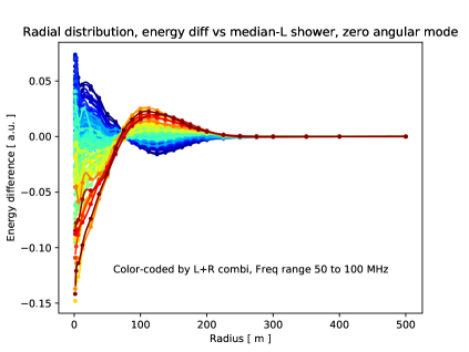
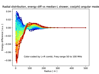
Thus, seeing a clear difference in footprint shape, we conclude that the footprints contain measurable information on at least the parameter . If this is not fully degenerate with the changes in footprint shape from a varying , this must be measurable in practice with a very dense array such as SKA.
4 Result of simulated reconstruction
We show the result of a typical simulated reconstruction of in the full frequency range, and of the parameter . The former is done on an ensemble spanning a range of in ; the latter is done on the ensemble at constant .
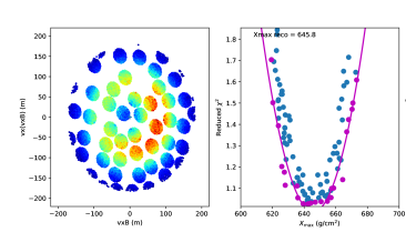
4.1 Reconstruction of in the 50 to 350 MHz frequency band
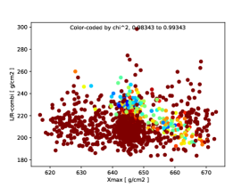
The -reconstruction is shown in Fig. 4. Variations in and have not been used here, as in the LOFAR -reconstruction. It gives a fitted value of that is within of the true value. A typical accuracy for reconstructed in this way is 6 to .
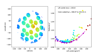
4.2 Reconstruction of a sensitive parameter in the 50 to 100 MHz band
In Fig. 5 we show the result of reconstructing the parameter from equation 4. Note that the reconstruction was done with the fixed- ensemble. Again, the versus shows a clear minimum, well fitted by a parabola. The fitted value is close to the real value of .
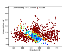
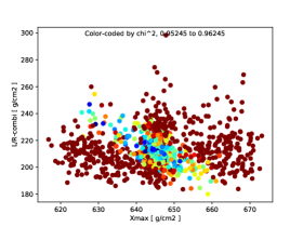
In a realistic measurement, we have to infer , , and (or a combination of them) simultaneously. For a first test of the capabilities to distinguish them, we have simulated additional showers in a wider range, and plotted their value of versus , color-coded by the reduced of their fit. Results for three showers are shown in Fig. 6; the color scale has been capped at a value not far above the minimum, to demonstrate the region where near-optimal fits are found. We find a ‘valley’ along a slanted line in these plots, where a higher and a lower or vice versa can produce nearly the same fit quality close to the optimum. Nevertheless, having determined from the full frequency band to about , we can already distinguish low, medium, and high values of . Extending this analysis to the full bandwidth has the potential of significantly improving on this result.
5 Summary
We have demonstrated cosmic-ray air shower measurement capabilities of SKA beyond what is possible at current radio observatories. To this end we have simulated the measurement process by passing simulated radio signals through the SKALA2 antenna model, adding realistic sky noise levels, and measuring pulse energies around their maximum.
In the three-parameter description of the longitudinal distribution of particles by , , and , we find that the radio footprint is sensitive to (as was already known) and to a linear combination of and which we denoted by . Using an ensemble of showers at a fixed , and restricting the bandwidth to to , we have seen that this combination of and can be reliably reconstructed in the same way as was already done for . Given a wider ensemble and results from the full frequency range, we can in this limited setup already distinguish between low, medium, and high values of .
The present analysis serves as a first exploration of the capabilities of a very densely instrumented radio telescope like SKA. Therefore, the results found here are only a lower bound to the precision that can be achieved. Measuring longitudinal shower parameters beyond , for individual showers, is not readily available at cosmic ray observatories in general. Thus, the ability to do this with SKA would once more demonstrate the value of radio measurements in detailed studies of air showers.
Acknowledgements
We acknowledge funding from the European Research Council under the European Union’s Horizon 2020 research and innovation programme (grant agreement n. 640130). TNGT acknowledges funding from Vietnam National Foundation for Science and Technology Development (NAFOSTED) under grant number 103.01-2019.378. ST acknowledges funding from the Khalifa University Startup grant, project code 8474000237-FSU-2020-13.
References
- [1] G. Tan et al., The square kilometre array baseline design v2.0, in 2015 1st URSI Atlantic Radio Science Conference (URSI AT-RASC), pp. 1–1, 2015.
- [2] M. P. van Haarlem et al., LOFAR: The Low Frequency Array, Astronomy and Astrophysics 556 (2013) A2.
- [3] A. Corstanje et al., Depth of shower maximum and mass composition of cosmic rays from 50 PeV to 2 EeV measured with the LOFAR radio telescope, Phys. Rev. D 103 (May, 2021) 102006.
- [4] S. Buitink et al., A large light-mass component of cosmic rays at electronvolts from radio observations, Nature (Mar, 2016) 70 .
- [5] S. Buitink et al., Constraining the cosmic-ray mass composition by measuring the shower length with SKA, These proceedings (2022).
- [6] S. Andringa, R. Conceição, and M. Pimenta, Mass composition and cross-section from the shape of cosmic ray shower longitudinal profiles, Astroparticle Physics 34 (2011), no. 6 360–367.
- [7] D. Heck et al., CORSIKA: a Monte Carlo code to simulate extensive air showers. Feb., 1998.
- [8] T. Huege, M. Ludwig, and C. W. James, Simulating radio emission from air showers with CoREAS, ARENA 2012, AIP Conf. Proc. 1535 (2013) 128–132.
- [9] T. Bergmann et al., One-dimensional hybrid approach to extensive air shower simulation, Astroparticle Physics 26 (2007), no. 6 420 – 432.
- [10] P. Virtanen et al., SciPy 1.0: Fundamental Algorithms for Scientific Computing in Python, Nature Methods 17 (2020) 261–272.
- [11] E. de Lera Acedo et al., SKALA, a log-periodic array antenna for the SKA-low instrument: design, simulations, tests and system considerations, Experimental Astronomy 39 (2015) 567 – 594.
- [12] E. Polisensky, LFmap: A low frequency sky map generating program, http://www.faculty.ece.vt.edu/swe/lwa/memo/lwa0111.pdf (2007).
- [13] K. Mulrey et al., Calibration of the LOFAR low-band antennas using the Galaxy and a model of the signal chain, Astroparticle Physics 111 (2019) 1–11.
- [14] S. Buitink et al., Method for high precision reconstruction of air shower using two-dimensional radio intensity profiles, Phys. Rev. D 90 (Oct, 2014) 082003.