NAISR: A 3D Neural Additive Model
for Interpretable Shape Representation

Abstract

Deep implicit functions (DIFs) have emerged as a powerful paradigm for many computer vision tasks such as 3D shape reconstruction, generation, registration, completion, editing, and understanding. However, given a set of 3D shapes with associated covariates there is at present no shape representation method which allows to precisely represent the shapes while capturing the individual dependencies on each covariate. Such a method would be of high utility to researchers to discover knowledge hidden in a population of shapes. For scientific shape discovery, we propose a 3D Neural Additive Model for Interpretable Shape Representation (NAISR) which describes individual shapes by deforming a shape atlas in accordance to the effect of disentangled covariates. Our approach captures shape population trends and allows for patient-specific predictions through shape transfer. NAISR is the first approach to combine the benefits of deep implicit shape representations with an atlas deforming according to specified covariates. We evaluate NAISR with respect to shape reconstruction, shape disentanglement, shape evolution, and shape transfer on three datasets: 1) Starman, a simulated 2D shape dataset; 2) the ADNI hippocampus 3D shape dataset; and 3) a pediatric airway 3D shape dataset. Our experiments demonstrate that NAISR achieves excellent shape reconstruction performance while retaining interpretability. Our code is available at https://github.com/uncbiag/NAISR.

1 Introduction

Deep implicit functions (DIFs) have emerged as efficient representations of 3D shapes (Park et al., 2019; Novello et al., 2022; Mescheder et al., 2019; Yang et al., 2021), deformation fields (Wolterink et al., 2022), images and videos (Sitzmann et al., 2020), graphs, and manifolds (Grattarola & Vandergheynst, 2022). For example, DeepSDF (Park et al., 2019) represents shapes as the level set of a signed distance field (SDF) with a neural network. In this way, 3D shapes are compactly represented as continuous and differentiable functions with infinite resolution. In addition to representations of geometry such as voxel grids (Wu et al., 2016; 2015; 2018), point clouds (Achlioptas et al., 2018; Yang et al., 2018; Zamorski et al., 2020) and meshes (Groueix et al., 2018; Wen et al., 2019; Zhu et al., 2019), DIFs have emerged as a powerful paradigm for many computer vision tasks. DIFs are used for 3D shape reconstruction (Park et al., 2019; Mescheder et al., 2019; Sitzmann et al., 2020), generation (Gao et al., 2022), registration (Deng et al., 2021; Zheng et al., 2021; Sun et al., 2022; Wolterink et al., 2022), completion (Park et al., 2019), editing (Yang et al., 2022a) and understanding (Palafox et al., 2022).

Limited attention has been paid to shape analysis with DIFs. Specifically, given a set of 3D shapes with a set of covariates attributed to each shape, a shape representation method is still desired which can precisely represent shapes and capture dependencies among a set of shapes. There is currently no shape representation method that can quantitatively capture how covariates geometrically and temporally affect a population of 3D shapes; neither on average nor for an individual. However, capturing such effects is desirable as it is often difficult and sometimes impossible to control covariates (such as age, sex, and weight) when collecting data. Further, understanding the effect of such covariates is frequently a goal of medical studies. Therefore, it is critical to be able to disentangle covariate shape effects on the individual and the population-level to better understand and describe shape populations. Our approach is grounded in the estimation of a shape atlas (i.e., a template shape) whose deformation allows to capture covariate effects and to model shape differences. Taking the airway as an example, a desired atlas representation should be able to answer the following questions:

• Given an atlas shape, how can one accurately represent shapes and their dependencies?

• Given the shape of an airway, how can one disentangle covariate effects from each other?

• Given a covariate, e.g., age, how does an airway atlas change based on this covariate?

• Given a random shape, how will the airway develop after a period of time?

To answer these questions, we propose a Neural Additive Interpretable Shape Representation (NAISR), an interpretable way of modeling shapes associated with covariates via a shape atlas. Table 1 compares NAISR to existing shape representations with respect to the following properties:

• Implicit relates to how a shape is described. Implicit representations are desirable as they naturally adapt to different resolutions of a shape and also allow shape completion (i.e., reconstructing a complete shape from a partial shape, which is common in medical scenarios) with no additional effort.

• Deformable captures if a shape representation results in point correspondences between shapes, e.g., via a displacement field. Specifically, we care about point correspondences between the target shapes and the atlas shape. A deformable shape representation helps to relate different shapes.

• Disentangleable indicates whether a shape representation can disentangle individual covariate effects for a shape. These covariate-specific effects can then be composed to obtain the overall displacement of an atlas/template shape.

• Evolvable denotes whether a shape representation can evolve the shape based on changes of a covariate, capturing the influence of individual covariates on the shape. An evolvable atlas statistically captures how each covariate influences the shape population, e.g., in scientific discovery scenarios.

• Transferable indicates whether shape changes can be transferred to a given shape. E.g., one might want to edit an airway based on a simulated surgery and predict how such a surgical change manifests later in life.

• Interpretable indicates a shape representation that is simultaneously deformable, disentangleable, evolvable, and transferable. Such an interpretable model is applicable to tasks ranging from the estimation of disease progression to assessing the effects of normal aging or weight gain on shape.

NAISR is the first implicit shape representation method to investigate an atlas-based representation of 3D shapes in a deformable, disentangleable, transferable and evolvable way. To demonstrate the generalizability of NAISR, we test NAISR on a simulated dataset and two realistic medical datasets : 1) Starman, a simulated 2D shape dataset (Bône et al., 2020); 2) the ADNI hippocampus 3D shape dataset (Jack Jr et al., 2008); and 3) a pediatric airway 3D shape dataset. We quantitatively demonstrate superior performance over the baselines.

Method	Implicit	Deformable	Disentangleable	Evolvable	Transferable	Interpretable
ConditionalTemplate (Dalca et al., 2019)	✗	✓	✗	✓	✗	✗
3DAttriFlow (Wen et al., 2022)	✗	✓	✗	✓	✗	✗
DeepSDF (Park et al., 2019)	✓	✗	✗	✗	✗	✗
A-SDF (Mu et al., 2021)	✓	✗	✗	✓	✓	✗
DIT (Zheng et al., 2021), DIF (Deng et al., 2021), NDF (Sun et al., 2022)	✓	✓	✗	✗	✗	✗
NASAM (Wei et al., 2022)	✓	✓	✗	✓	✗	✗
Ours (NAISR)	✓	✓	✓	✓	✓	✓

Table 1: Comparison of shape representations based on the desirable properties discussed in Section 1. A ✓indicates that a model has a property; a ✗indicates that it does not. Only NAISR has all the desired properties.

2 Related Work

We introduce the three most related research directions here. A more comprehensive discussion of related work is available in Section S.1 of the supplementary material.

Deep Implicit Functions.

Compared with geometry representations such as voxel grids (Wu et al., 2016; 2015; 2018), point clouds (Achlioptas et al., 2018; Yang et al., 2018; Zamorski et al., 2020) and meshes (Groueix et al., 2018; Wen et al., 2019; Zhu et al., 2019), DIFs are able to capture highly detailed and complex 3D shapes using a relatively small amount of data (Park et al., 2019; Mu et al., 2021; Zheng et al., 2021; Sun et al., 2022; Deng et al., 2021). They are based on classical ideas of level set representations (Sethian, 1999; Osher & Fedkiw, 2005); however, whereas these classical level set methods represent the level set function on a grid, DIFs parameterize it as a continuous function, e.g., by a neural network. Hence, DIFs are not reliant on meshes, grids, or a discrete set of points. This allows them to efficiently represent natural-looking surfaces (Gropp et al., 2020; Sitzmann et al., 2020; Niemeyer et al., 2019). Further, DIFs can be trained on a diverse range of data (e.g., shapes and images), making them more versatile than other shape representation methods. This makes them useful in applications ranging from computer graphics, to virtual reality, and robotics (Gao et al., 2022; Yang et al., 2022a; Phongthawee et al., 2022; Shen et al., 2021). We therefore formulate NAISR based on DIFs.

Point Correspondences.

Establishing point correspondences is important to help experts to detect, understand, diagnose, and track diseases. Recently, ImplicitAtlas (Yang et al., 2022b), DIF-Net (Deng et al., 2021), DIT (Zheng et al., 2021), and NDF (Sun et al., 2022) were proposed to capture point correspondence within implicit shape representations. Dalca et al. (Dalca et al., 2019) use templates conditioned on covariates for image registration. However, they did not explore covariate-specific deformations, shape representations or shape transfer. Currently no continuous shape representation which models the effects of covariates exists. NAISR will provide a model with such capabilities.

Explainable Artificial Intelligence.

The goal of eXplainable Artificial Intelligence (XAI) is to provide human-understandable explanations for decisions and actions of a AI model. Various flavors of XAI exist, including counterfactual inference (Berrevoets et al., 2021; Moraffah et al., 2020; Thiagarajan et al., 2020; Chen et al., 2022), attention maps (Zhou et al., 2016; Jung & Oh, 2021; Woo et al., 2018), feature importance (Arik & Pfister, 2021; Ribeiro et al., 2016; Agarwal et al., 2020), and instance retrieval (Crabbe et al., 2021). NAISR is inspired by neural additive models (NAMs) (Agarwal et al., 2020) which in turn are inspired by generalized additive models (GAMs) (Hastie, 2017). NAMs are based on a linear combination of neural networks each attending to a single input feature, thereby allowing for interpretability. NAISR extends this concept to interpretable 3D shape representations. This is significantly more involved as, unlike for NAMs and GAMs, we are no longer dealing with scalar values, but with 3D shapes. NAISR will provide interpretable results by capturing spatial deformations with respect to an estimated atlas shape such that individial covariate effects can be distinguished.

3 Method

This section disccuses our NAISR model and how we obtain the desired model properties of Section 1.

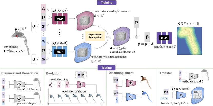
Figure 1: Neural Additive Implicit Shape Representation. During training we learn the template $\mathcal{T}$ and the multi-layer perceptrons (MLPs) $\{g_{i}\}$ predicting the covariate-wise displacement fields $\{\mathbf{d}_{i}\}$. The displacement fields are added to obtain the overall displacement field $\mathbf{d}$ defined in the target space; $\mathbf{d}$ provides the displacement between the deformed template shape $\mathcal{T}$ and the target shape. Specifically the template shape is queried not at its original coordinates $\mathbf{p}$, but at $\tilde{\mathbf{p}}=\mathbf{p}+\mathbf{d}$ effectively spatially deforming the template. At test time we evaluate the trained MLPs for shape reconstruction, evolution, disentanglement, and shape transfer.

3.1 Problem Description

Consider a set of shapes $\mathcal{S}=\{\mathcal{S}^{k}\}$ where each shape $\mathcal{S}^{k}$ has an associated vector of covariates $\mathbf{c}=[c_{1},...,c_{i},...,c_{N}]$ (e.g., age, weight, sex). Our goal is to obtain a representation which describes the entire set $\mathcal{S}$ while accounting for the covariates. Our approach estimates a template shape, $\mathcal{T}$ (the shape atlas), which approximates $\mathcal{S}$. Specifically, $\mathcal{T}$ is deformed based on a set of displacement fields $\{\mathcal{D}^{k}\}$ such that the individual shapes $\{\mathcal{S}^{k}\}$ are approximated well by the transformed template.

A displacement field $\mathcal{D}^{k}$ describes how a shape is related to the template shape $\mathcal{T}$. The factors that cause this displacement may be directly observed or not. For example, observed factors may be covariates such as subject age, weight, or sex; i.e., $\mathbf{c}_{k}$ for subject $k$. Factors that are not directly observed may be due to individual shape variation, unknown or missing covariates, or variations due to differences in data acquisition or data preprocessing errors. We capture these not directly observed factors by a latent code $\mathbf{z}$. The covariates $\mathbf{c}$ and the latent code $\mathbf{z}$ then contribute jointly to the displacement $\mathcal{D}$ with respect to the template shape $\mathcal{T}$.

Inspired by neural additive (Agarwal et al., 2020) and generalized additive (Hastie, 2017) models, we assume the overall displacement field is the sum of displacement fields that are controlled by individual covariates: $\mathcal{D}=\Sigma_{i}\mathcal{D}_{i}$. Here, $\mathcal{D}_{i}$ is the displacement field controlled by the i-th covariate, $c_{i}$. This results by construction in an overall displacement $\mathcal{D}$ that is disentangled into several sub-displacement fields $\{\mathcal{D}_{i}\}$.

3.2 Model Formulation

Figure 1 gives an overview of NAISR. To obtain a continuous atlas representation, we use DIFs to represent both the template $\mathcal{T}$ and the displacement field $\mathcal{D}$. The template shape $\mathcal{T}$ is represented by a signed distance function, where the zero level set $\{\mathbf{p}\in\mathbb{R}^{3}|\mathcal{T}(\mathbf{p})=0\}$ captures the desired template shape. A displacement $\mathcal{D}_{i}$ of a particular point $\mathbf{p}$ can also be represented as a function $\mathbf{d}_{i}=f_{i}(\mathbf{p},c_{i},\mathbf{z})\in\mathbb{R}^{3}$. We use SIREN (Sitzmann et al., 2020) as the backbone for $\mathcal{T}(\cdot)$ and $\{f_{i}(\cdot)\}$. Considering that the not directly observed factors might influence the geometry of all covariate-specific networks, we make the latent code, $\mathbf{z}$, visible to all subnetworks $\{f_{i}(\cdot)\}$. We normalize the covariates so that they are centered at zero. To assure that a zero covariate value results in a zero displacement we parameterize the displacement fields as $\mathbf{d}_{i}=g_{i}(\mathbf{p},c_{i},\mathbf{z})$ where

$$g_{i}(\mathbf{p},c_{i},\mathbf{z})=f_{i}(\mathbf{p},c_{i},\mathbf{z})-f_{i}(\mathbf{p},0,\mathbf{z})\,.$$ (1)

The sub-displacement fields are added to obtain the overall displacement field

$$\mathbf{d}=g(\mathbf{p},\mathbf{c},\mathbf{z})=\sum_{i=1}^{N}g_{i}(\mathbf{p},c_{i},\mathbf{z})\,.$$ (2)

We then deform the template shape $\mathcal{T}$ to obtain an implicit representation of a target shape

$$s=\Phi(\mathbf{p},\mathbf{c},\mathbf{z})=\mathcal{T}(\tilde{\mathbf{p}})=\mathcal{T}(\mathbf{p}+\sum_{i=1}^{N}g_{i}(\mathbf{p},c_{i},\mathbf{z}))\,,$$ (3)

where $\mathbf{p}$ is a point in the source shape space, e.g., a point on the surface of shape $\mathcal{S}_{i}$ and $\tilde{\mathbf{p}}$ represents a point in the template shape space, e.g., a point on the surface of the template shape $\mathcal{T}$. To investigate how an individual covariate $c_{i}$ affects a shape we can simply extract the zero level set of

$$s_{i}=\Phi_{i}(\mathbf{p},c_{i},\mathbf{z})=\mathcal{T}(\mathbf{p}+\mathbf{d}_{i})=\mathcal{T}(\mathbf{p}+g_{i}(\mathbf{p},c_{i},\mathbf{z}))\,.$$ (4)

3.3 Training

Losses.

All our losses are ultimately summed over all shapes of the training population with the appropriate covariates $\mathbf{c}_{k}$ and shape code $\mathbf{z}_{k}$ for each shape $\mathcal{S}^{k}$. For ease of notation, we describe them for individual shapes. For each shape, we sample on-surface and off-surface points. On-surface points have zero signed distance values and normal vectors extracted from the gold standard mesh. Off-surface points have non-zero signed distance values but no normal vectors. Our reconstruction losses follow Sitzmann et al. (2020); Novello et al. (2022). For points on the surface, the losses are

$$\mathcal{L}_{\mathrm{on}}(\Phi,\mathbf{c},\mathbf{z})=\int_{\mathcal{S}}\lambda_{1}\underbrace{\left\|\left|\nabla_{\mathbf{p}}\Phi(\mathbf{p},\mathbf{c},\mathbf{z})\right|-1\right\|}_{\mathcal{L}_{\text{Eikonal}}}\\ +\lambda_{2}\underbrace{\|\Phi(\mathbf{p},\mathbf{c},\mathbf{z})\|}_{\mathcal{L}_{\text{Dirichlet}}}+\lambda_{3}\underbrace{\left(1-\left\langle\nabla_{\mathbf{p}}\Phi(\mathbf{p},\mathbf{c},\mathbf{z}),\mathbf{n}(\mathbf{p})\right\rangle\right)}_{\mathcal{L}_{\text{Neumann}}}d\mathbf{p}\,,$$ (5)

where $\mathbf{n}(\mathbf{p})$ is the normal vector at $\mathbf{p}$ and $\langle\cdot\rangle$ denotes cosine similarity. For off-surface points, we use

$$\mathcal{L}_{\mathrm{off}}(\Phi,\mathbf{c},\mathbf{z})=\int_{\Omega\backslash\mathcal{S}}\lambda_{4}\underbrace{|\Phi(\mathbf{p},\mathbf{c},\mathbf{z})-s_{tgt}(\mathbf{p})|}_{\mathcal{L}_{\text{Dirichlet}}}+\lambda_{5}\underbrace{\left\|\left|\nabla_{\mathbf{p}}\Phi(\mathbf{p},\mathbf{c},\mathbf{z})\right|-1\right\|}_{\mathcal{L}_{\text{Eikonal}}}d\mathbf{p}\,,$$ (6)

where $s_{tgt}(\mathbf{p})$ is the signed distance value at $\mathbf{p}$ corresponding to a given target shape. Similar to (Park et al., 2019; Mu et al., 2021) we penalize the squared $L^{2}$ norm of the latent code $z$ as

$$\mathcal{L}_{\mathrm{lat}}(\mathbf{z})=\lambda_{6}\frac{1}{\sigma^{2}}\left\|\bm{z}\right\|_{2}^{2}\,.$$ (7)

As a result, our overall loss (for a given shape) is

$$\mathcal{L}(\Phi,\mathbf{c},\mathbf{z})=\underbrace{\mathcal{L}_{\mathrm{lat}}(\mathbf{z})}_{\text{as regularizer}}+\underbrace{\mathcal{L}_{\mathrm{on}}(\Phi,\mathbf{c},\mathbf{z})+\mathcal{L}_{\mathrm{off}}(\Phi,\mathbf{c},\mathbf{z})}_{\text{for reconstrution}}\,,$$ (8)

where the parameters of $\Phi$ and $\mathbf{z}$ are trainable.

3.4 Testing

As shown in Figure 1, our proposed NAISR is designed for shape reconstruction, shape disentanglement, shape evolution, and shape transfer. Further, NAISR also allows for shape interpolation, shape completion, and shape correspondence by design as in (Zheng et al., 2021; Sun et al., 2022).

Shape Reconstruction and Generation.

As illustrated in the inference section in Figure 1, a shape $s_{tgt}$ is given and the goal is to recover its corresponding latent code $\mathbf{z}$ and the covariates $\mathbf{c}$. To estimate these quantities, the network parameters stay fixed and we optimize over the covariates $\mathbf{c}$ and the latent code $\mathbf{z}$ which are both randomly initialized (Park et al., 2019; Mu et al., 2021). Specifically, we solve the optimization problem

$$\hat{\mathbf{c}},\hat{\mathbf{z}}=\underset{\mathbf{c},\mathbf{z}}{\arg\min}~{}\mathcal{L}(\Phi,\mathbf{c},\mathbf{z})\,.$$ (9)

In clinical scenarios, the covariates $\mathbf{c}$ might be known (e.g., recorded age or weight at imaging time). In this case, we only infer the latent code $\mathbf{z}$ by the optimization

$$\hat{\mathbf{z}}=\underset{\mathbf{z}}{\arg\min}~{}\mathcal{L}(\Phi,\mathbf{c},\mathbf{z})\,.$$ (10)

A new patient shape with different covariates can be generated by extracting the zero level set of $\Phi(\mathbf{p},\mathbf{c}_{\mathrm{new}},\hat{\mathbf{z}})$.

Shape Evolution.

Shape evolution along covariates $\{c_{i}\}$ is desirable in shape analysis to obtain knowledge of disease progression or population trends in the shape population $\mathcal{S}$. For a time-varying covariate $(c_{i}^{0},...,c_{i}^{t},...,c_{i}^{T})$, we obtain the corresponding shape evolution by $(\Phi_{i}(\mathbf{p},c_{i}^{0},\hat{\mathbf{z}}),...,\Phi_{i}(\mathbf{p},c_{i}^{t},\hat{\mathbf{z}}),...,\Phi_{i}(\mathbf{p},c_{i}^{T},\hat{\mathbf{z}}))$. If some covariates are correlated (e.g., age and weight), we can first obtain a reasonable evolution of the covariates $(\mathbf{c}^{0},...,\mathbf{c}^{t},...,\mathbf{c}^{T})$ and the corresponding shape evolution as $(\Phi(\mathbf{p},\mathbf{c}^{0},\hat{\mathbf{z}}),...,\Phi(\mathbf{p},\mathbf{c}^{t},\hat{\mathbf{z}}),...,\Phi(\mathbf{p},\mathbf{c}^{T},\hat{\mathbf{z}}))$. By setting $\hat{\mathbf{z}}$ to $\mathbf{0}$, one can observe how a certain covariate influences the shape population on average.

Shape Disentanglement.

As shown in the disentanglement section in Figure 1, the displacement for a particular covariate $c_{i}$ displaces point $\mathbf{p}$ in the source space to $\mathbf{p}+\mathbf{d}_{i}$ in the template space for a given or inferred $\hat{\mathbf{z}}$ and $c_{i}$. We obtain the corresponding signed distance field as

$$s_{i}=\Phi_{i}(\mathbf{p},c_{i},\hat{\mathbf{z}})=\mathcal{T}(\mathbf{p}+\mathbf{d}_{i})=\mathcal{T}(\mathbf{p}+g_{i}(\mathbf{p},c_{i},\hat{\mathbf{z}}))\,.$$ (11)

As a result, the zero level sets of $\{\Phi_{i}(\cdot)\}$ represent shapes warped by the sub-displacement fields controlled by $c_{i}$.

Shape Transfer.

We use the following clinical scenario to introduce the shape transfer task. Suppose a doctor has conducted simulated surgery on an airway shape with the goal of previewing treatment effects on the shape after a period of time. This question can be answered by our shape transfer approach. Specifically, as shown in the transfer section in Figure 1, after obtaining the inferred latent code $\hat{\mathbf{z}}$ and covariates $\hat{\mathbf{c}}$ from reconstruction, one can transfer the shape from the current covariates $\hat{\mathbf{c}}$ to new covariates $\hat{\mathbf{c}}+{\Delta\mathbf{c}}$ with $\Phi(\mathbf{p},\hat{\mathbf{c}}+\Delta{\mathbf{c}},\hat{\mathbf{z}})$. As a result, the transferred shape is a prediction of the outcome of the simulated surgery; it is the zero level set of $\Phi(\mathbf{p},\hat{\mathbf{c}}+\Delta{\mathbf{c}},\hat{\mathbf{z}})$. In more general scenarios, the covariates are unavailable but it is possible to infer them from the measured shapes themselves (see Eqs. 9-10). Therefore, in shape transfer we are not only evolving a shape, but may also first estimate the initial state to be evolved.

4 Experiments

We evaluate NAISR in terms of shape reconstruction, shape disentanglement, shape evolution, and shape transfer on three datasets: 1) Starman, a simulated 2D shape dataset used in (Bône et al., 2020); 2) the ADNI hippocampus 3D shape dataset (Petersen et al., 2010); and 3) a pediatric airway 3D shape dataset. Starman serves as the simplest and ideal scenario where sufficient noise-free data for training and evaluating the model is available. While the airway and hippocampus datasets allow for testing on real-world problems of scientific shape analysis, which motivates NAISR.

We can quantitatively evaluate NAISR for shape reconstruction and shape transfer because our dataset contains longitudinal observations. For shape evolution and shape disentanglement, we provide visualizations of shape extrapolations in covariate space to demonstrate that our method can learn a reasonable representation of the deformations governed by the covariates.

Implementation details and ablation studies are available in Section S.3.1 and Section S.3.2 in the supplementary material.

4.1 Dataset and Experimental Protocol

Starman Dataset. This is a synthetic 2D shape dataset obtained from a predefined model as illustrated in Section S.2.1 without additional noise. As shown in Fig. S.4, each starman shape is synthesized by imposing a random deformation representing individual-level variation to the template starman shape. This is followed by a covariate-controlled deformation to the individualized starman shape, representing different poses produced by a starman. 5041 shapes from 1000 starmans are synthesized as the training set; 4966 shapes from another 1000 starmans are synthesized as a testing set.

ADNI Hippocampus Dataset. These hippocampus shapes were obtained from the Alzheimer’s Disease Neuroimaging Initiative (ADNI) database . The dataset consists of 1632 hippocampus segmentations from magnetic resonance (MR) images. We use an 80%-20% train-test split by patient (instead of shapes); i.e., a given patient cannot simultaneously be in the train and the test set, and therefore no information can leak between these two sets. As a result, the training set consists of 1297 shapes while the testing set contains 335 shapes. Each shape is associated with 4 covariates (age, sex, AD, education length). AD is a binary variable indicating whether a person has Alzheimer disease.

Pediatric Airway Dataset. This dataset contains 357 upper airway shapes to evaluate our method. These shapes are obtained from automatic airway segmentations of computed tomography (CT) images of children with a radiographically normal airway. These 357 airway shape are from 263 patients, 34 of whom have longitudinal observations and 229 of whom have only been observed once. We use a 80%-20% train-test split by patient (instead of shapes). Each shape has 3 covariates (age, weight, sex).

More details, including demographic information, visualizations, and preprocessing steps of the datasets are available in Section S.2 in the supplementary material.

Comparison Methods.

For shape reconstruction of unseen shapes, we compare our method on the test set with DeepSDF (Park et al., 2019) A-SDF (Mu et al., 2021) DIT (Zheng et al., 2021) and NDF (Sun et al., 2022). For shape transfer, we compare our method with A-SDF (Mu et al., 2021) because other comparison methods cannot model covariates as summarized in Table  1.

Metrics.

For evaluation, all target shapes and reconstructed meshes are normalized to a unit sphere to assure that large shapes and small shapes contribute equally to error measurements. We use the Hausdorff distance, Chamfer distance, and earth mover’s distance to evaluate the performance of our shape reconstructions. For shape transfer, considering that a perfectly consistent image acquisition process is impossible for different observations (e.g., head positioning might slightly vary across timepoints for the airway data), we visualize the transferred shapes and evaluate based on the difference between the volumes of the reconstructed shapes and the target shapes on the hippocampus and airway dataset.

4.2 Shape Reconstruction

The goal of our shape reconstruction experiment is to demonstrate that NAISR can provide competitive reconstruction performance while providing interpretability. Table  2 shows the quantitative evaluations and demonstrates the excellent reconstruction performance of NAISR. Figure 2 visualizes reconstructed shapes. We observe that implicit shape representations can complete missing shape parts which can benefit further shape analysis. A-SDF (Mu et al., 2021) works well for representing Starman shapes but cannot reconstruct real 3D medical shapes successfully. The reason might be the time span of our longitudinal data for each patient is far shorter than the time span across the entire dataset, mixing individual differences and covariate-controlling differences. A-SDF may fail to disentangle such mixed effects (from individuals and covariates), but instead memorizes training shapes by their covariates $\mathbf{c}$. In contrast, the additive architecture of NAISR prevents the model from memorizing training shapes through covariates $\mathbf{c}$. More discussions are available at Section S.3.3 in the supplementary material.

	Starman						ADNI Hippocampus						Pediatric Airway
	CD $\downarrow$		EMD $\downarrow$		HD $\downarrow$		CD $\downarrow$		EMD $\downarrow$		HD $\downarrow$		CD $\downarrow$		EMD $\downarrow$		HD $\downarrow$
	$\mu$	M	$\mu$	M	$\mu$	M	$\mu$	M	$\mu$	M	$\mu$	M	$\mu$	M	$\mu$	M	$\mu$	M
DeepSDF	0.117	0.105	1.941	1.887	6.482	6.271	0.157	0.140	2.098	2.035	9.762	9.276	0.077	0.052	1.401	1.266	10.765	9.446
A-SDF	0.173	0.092	2.01	1.668	8.806	6.949	1.094	1.162	7.156	7.667	25.092	25.938	2.647	1.178	10.302	9.068	47.172	37.835
A-SDF (c)	0.049	0.043	1.298	1.261	5.388	4.964	0.311	0.294	3.136	3.099	13.852	13.003	0.852	0.226	4.090	2.890	30.848	21.965
DIT	0.281	0.181	2.727	2.497	10.295	8.442	0.156	0.142	2.096	2.054	9.465	9.123	0.094	0.049	1.414	1.262	11.524	10.228
NDF	1.086	0.736	5.364	4.821	21.098	19.705	0.253	0.213	2.699	2.58	11.328	10.947	0.238	0.117	2.174	1.737	14.950	12.516
Ours	0.111	0.072	1.709	1.515	7.951	7.141	0.174	0.153	2.258	2.191	10.019	9.521	0.067	0.039	1.233	1.132	10.333	8.404
Ours (c)	0.049	0.036	1.276	1.156	5.051	4.666	0.126	0.116	1.847	1.81	8.586	8.153	0.084	0.044	1.345	1.190	10.719	8.577

Table 2: Quantitative evaluation of shape reconstruction. $\mathrm{CD}=$ Chamfer distance. $\mathrm{EMD}=$ Earth mover’s distance. $\mathrm{HD}=$ Hausdorff distance. All metrics are multiplied by $10^{2}$. Bold red values indicate the best scores across all methods. Bold black values indicate the 2nd best scores of all methods. Ours means the covariates were inferred during testing (see Equation 9). Ours(c) means the covariates are used as input during inference (see Equation 10). $\mu$ and M indicate the mean and median of the measurements on the testing shapes respectively. NAISR performs well for all three reconstruction tasks while allowing for interpretability.

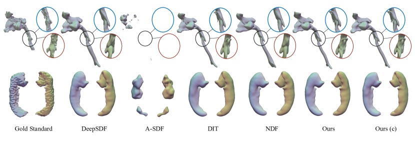
Figure 2: Visualizations of airway and hippocampus reconstruction with different methods. The red and blue circles show the structure in the black circle from two different views. Hippocampus shapes are plotted with two $180^{\circ}$-flipped views. NAISR can produce detailed and accurate reconstructions as well as impute missing airway parts. More visualizations are available in Section S.3.3 of the supplementary material.

4.3 Shape Transfer

Table 4 shows an airway shape transfer example for a cancer patient who was scanned 11 times. We observe that our method can produce complete transferred shapes that correspond well with the measured shapes. Table 3 shows quantitative results for the volume differences between our transferred shapes and the gold standard shapes. Our method performs best on the real datasets while A-SDF (the only other model supporting shape transfer) works slightly better on the synthetic Starman dataset. Our results demonstrate that NAISR is capable of transferring shapes to other timepoints $\mathcal{S}^{t}$ from a given initial state $\mathcal{S}^{0}$.

		Starman						ADNI Hippocampus		Pediatric Airway
	!	CD $\downarrow$		EMD $\downarrow$		HD $\downarrow$		VD $\downarrow$		VD $\downarrow$
!	w.C.	$\mu$	M	$\mu$	M	$\mu$	M	$\mu$	M	$\mu$	M
A-SDF	✗	0	0	0.009	0.008	0.036	0.034	0.518	0.488	81.07	82.92
A-SDF	✓	0	0	0.009	0.009	0.036	0.035	0.215	0.177	41.46	40.96
Ours	✗	0.003	0.002	0.025	0.023	0.094	0.077	0.086	0.063	12.82	8.84
Ours	✓	0.009	0.002	0.031	0.025	0.116	0.083	0.089	0.071	11.23	9.65

Table 3: Quantitative evaluation of shape transfer. Statistics of Volume Difference (VD, $cm^{3}$) between transferred shapes and gold standard shapes. w.C. abbreviates with covariates. A ✓in w.C. indicates the inference follows Equation 10. A ✗in w.C. indicates the inference follows Equation 9. Red bold scores indicate the best performance across all methods and bold scores indicate the 2nd best. NAISR results in significantly improved volume estimates for real medical shapes.

#time	0	1	2	3	4	5	6	7	8	9	10
$\{\mathcal{S}^{t}\}$

# time	0	1	2	3	4	5	6	7	8	9	10
age	154	155	157	159	163	164	167	170	194	227	233
weight	55.2	60.9	64.3	65.25	59.25	59.2	65.3	68	77.1	75.6	75.6
sex	M	M	M	M	M	M	M	M	M	M	M
p-vol	92.5	93.59	94.64	95.45	96.33	96.69	98.4	99.72	109.47	118.41	118.76
m-vol	86.33	82.66	63.23	90.65	98.11	84.35	94.14	127.45	98.81	100.17	113.84

Table 4: Airway shape transfer for a patient. Blue: gold standard shapes; red: transferred shapes with NAISR. The table below lists the covariates (age/month, weight/kg, sex) for the shapes above. P-vol(predicted volume) is the volume ($cm^{3}$) of the transferred shape by NAISR covariates following Equation 9. M-vol (measured volume) is the volume ($cm^{3}$) of the shapes based on the actual imaging. NAISR can capture the trend of growing volume with age and weight while producing clear, complete, and topology-consistent shapes. Note that measured volumes may differ depending on the CT imaging field of view. More visualizations are available in Section S.3.4 in the supplementary material.

4.4 Shape Disentanglement and Evolution

Figure 3 shows that NAISR is able to extrapolate reasonable shape changes when varying covariates. These results illustrate the capabilities of NAISR for shape disentanglement and to capture shape evolutions. A-SDF and NAISR both produce high-quality Starman shapes because the longitudinal data is sufficient for the model to discover the covariate space. However, for real data, only NAISR can produce realistic 3D hippocampi and airways reflecting the covariates’ influences on template shapes. Note that when evolving shapes along a single covariate $c_{i}$, the deformations from other covariates are naturally set to $\mathbf{0}$ by our model construction (see Section 3.2). As a result, the shapes in the yellow and green boxes in Figure 3 represent the disentangled shape evolutions along different covariates respectively. The shapes in the other grid positions can be extrapolated using $\Phi(\cdot)$. By inspecting the volume changes in the covariate space in Figure 3, we observe that age is more important for airway volume than weight, and Alzheimer disease influences hippocampal volume. These observations from our generated shapes are consistent with clinical expectations (Luscan et al., 2020; Gosche et al., 2002), suggesting that NAISR is able to extract hidden knowledge from data and is able to generate interpretable results directly as 3D shapes.

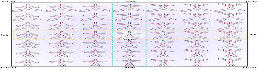
A-SDF, Starman

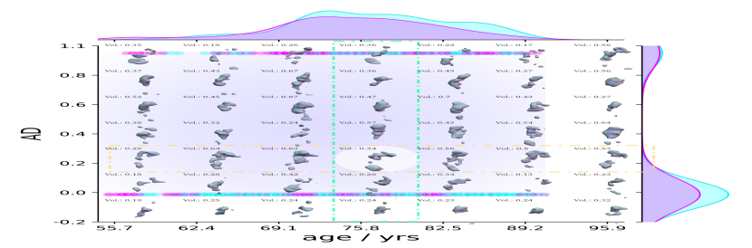
A-SDF, ADNI Hippocampus

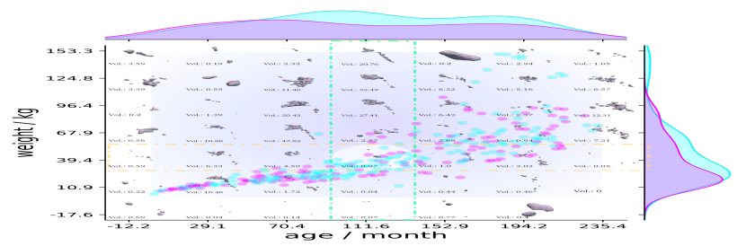
A-SDF, Pediatric Airway

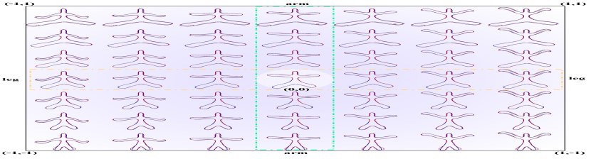
Ours, Starman

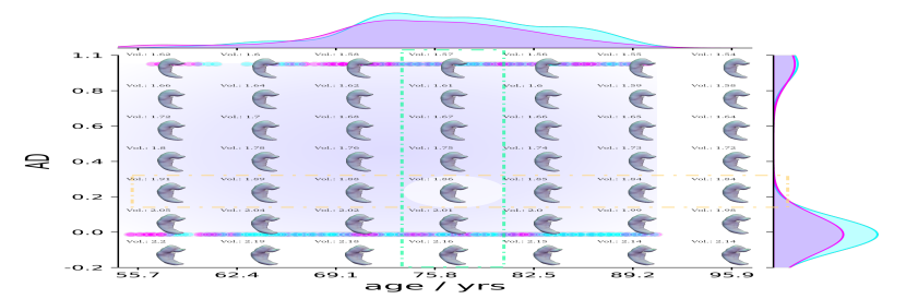
Ours, ADNI Hippocampus

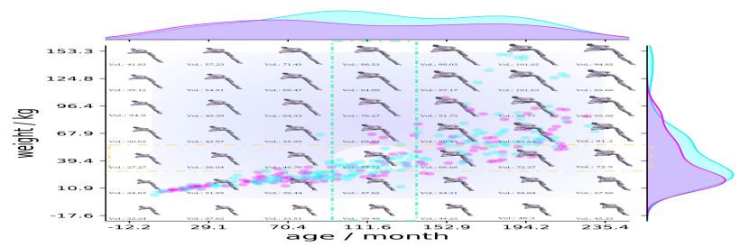
Ours, Pediatric Airway

Figure 3: Template shape extrapolation in covariate space using A-SDF and NAISR on three datasets. For the Starman shape extrapolations, the blue shapes are the groundtruth shapes and the red shapes are the reconstructions. The shapes in the middle white circles are the template shapes. The template shape is generated with zero latent code and is used to create a template covariate space. The shapes in the green and yellow boxes are plotted with $\{\Phi_{i}\}$, representing the disentangled shape evolutions along each covariate respectively. The purple shadows over the space indicate the covariate range that the dataset covers. Cyan points represent male and purple points female patients in the dataset. The points represent the covariates of all patients in the dataset. The colored shades at the boundary represent the covariate distributions stratified by sex. Example 3D shapes in the covariate space are visualized with their volumes ($cm^{3}$) below. NAISR is able to extrapolate the shapes in the covariate space given either an individualized latent code $\mathbf{z}$ or template latent code $\mathbf{0}$, whereas A-SDF struggles. The supplementary material provides more visualizations of individualized covariate spaces in Section S.3.5. (Best viewed zoomed.)

5 Conclusion

In this work, we proposed NAISR, a 3D neural additive model for interpretable shape representation. We tested NAISR on three different datasets and observed particularly good performance on real 3D medical datasets. Compared to other shape representation methods, NAISR 1) captures the effect of individual covariates on shapes; 2) can transfer shapes to new covariates, e.g., to infer anatomy development; and 3) can provide shapes based on extrapolated covariates. NAISR is the first approach combining deep implicit shape representations based on template deformation with the ability to account for covariates. We believe our work is an exciting start for a new line of research: interpretable neural shape models for scientific discovery. We discuss the limitations and future work of NAISR at Section S.4 in the supplementary material.

Reproducibility Statement

We are dedicated to ensuring the reproducibility of NAISR to facilitate more scientific discoveries on shapes. To assist researchers in replicating and building upon our work, we made the following efforts,

• Model & Algorithm: Our paper provides detailed descriptions of the model architectures (See Section 3), implementation details (See Section S.3.1), and ablation studies (See Section S.3.2). We have submitted our source code. The implementation of NAISR will be made publicly available.

• Datasets & Experiments: We provide extensive illustrations and visualizations for the datasets we used. To ensure transparency and ease of replication, the exact data processing steps, from raw data to processed input, are outlined at Section S.2 in the supplementary materials. We expect our thorough supplementary to ensure the reproducibility of our method and the understandability of our experiment results. We submit the code for synthesizing the 2D Starman dataset so that researchers can easily reproduce the results.

Supplementary Material for NAISR

Appendix S.1 Related Work

Deep Implicit Functions.

Point Correspondence.

Establishing point correspondences is important to help experts to detect, understand, diagnose, and track diseases. Recently, ImplicitAtlas (Yang et al., 2022b), DIF-Net (Deng et al., 2021), DIT (Zheng et al., 2021), and NDF (Sun et al., 2022) were proposed to capture point correspondence within implicit shape representations. Dalca et al. (Dalca et al., 2019) use templates conditioned on covariates for image registration. However, they did not explore covariate-specific deformations, shape representations or shape transfer. Currently, no continuous shape representation which models the effects of covariates exists. NAISR provides a model with such capabilities.

Disentangled Representation Learning.

Disentangled representation learning (DRL) has been explored in a variety of domains, including computer vision (Shoshan et al., 2021; Ding et al., 2020; Zhang et al., 2018b; a; Xu et al., 2021; Yang et al., 2020), natural language processing (John et al., 2018), and medical image analysis (Chartsias et al., 2019; Bercea et al., 2022). DRL has also emerged in the context of implicit representations as a promising approach for 3D computer vision. By disentangling the underlying factors of variation, such as object shape, orientation, and texture, DRL can facilitate more effective 3D object recognition, reconstruction, and manipulation (Stammer et al., 2022; Zhang et al., 2018b; a; Xu et al., 2021; Yang et al., 2020; 2022a; Gao et al., 2022; Tewari et al., 2022).

Besides DRL in computer vision, medical data is typically associated with various covariates which should be taken into account during analyses. Taking (Chu et al., 2022) as an example, when observing a tumor’s progression, it is difficult to know whether the variation of a tumor’s progression is due to time-varying covariates or due to treatment effects. Therefore, being able to disentangle different effects is highly useful for a representation to promote understanding and to be able to quantify the effect of covariates on observations. NAISR provides a disentangled representation and allows us to capture the shape effects of covariates.

Articulated Shapes.

There is significant research focusing on articulated shapes, mostly on humans (Palafox et al., 2021; Chen et al., 2021; Tretschk et al., 2020; Deng et al., 2020). There is also a line of work on articulated general objects, e.g., A-SDF (Mu et al., 2021) and NASAM (Wei et al., 2022). A-SDF (Mu et al., 2021) uses articulation as an additional input to control generated shapes, while NASAM (Wei et al., 2022) learns the latent space of articulation without articulation as supervision.

The aforementioned works on articulated objects assume that each articulation affects a separate object part. This is easy to observe, e.g., the angles of the two legs of a pair of eyeglasses. Hence, although A-SDF (Mu et al., 2021) and 3DAttriFlow (Wen et al., 2022) can disentangle articulations from geometry, they do not disentangle different covariates and their disentanglements are not composable. However, in medical scenarios, covariates often affect shapes in a more entangled and complex way, for example, a shape might simultaneously be influenced by sex, age, and weight. NAISR allows us to account for such complex covariate interactions.

Explainable Artificial Intelligence.

The goal of eXplainable Artificial Intelligence (XAI) is to provide human-understanable explanations for decisions and actions of an AI model. Various flavors of XAI exist, including counterfactual inference (Berrevoets et al., 2021; Moraffah et al., 2020; Thiagarajan et al., 2020; Chen et al., 2022), attention maps (Zhou et al., 2016; Jung & Oh, 2021; Woo et al., 2018), feature importance (Arik & Pfister, 2021; Ribeiro et al., 2016; Agarwal et al., 2020), and instance retrieval (Crabbe et al., 2021). NAISR is inspired by neural additive models (NAMs) (Agarwal et al., 2020) which in turn are inspired by generalized additive models (GAMs) (Hastie, 2017). NAMs are based on a linear combination of neural networks each attending to a single input feature. NAISR extends this concept to interpretable 3D shape representations. This is significantly more involved as, unlike for NAMs and GAMs, we are no longer dealing with scalar values, but with 3D shapes. NAISR provides interpretable results by capturing spatial deformations with respect to an estimated atlas shape such that individual covariate effects can be distinguished.

Appendix S.2 Dataset

S.2.1 Starman Dataset

Figure S.4 illustrates how each sample in the dataset is simulated. 5041 shapes from 1000 different starmans are simulated as the training set. 4966 shapes from another 1000 starmans are simulated as a testing set. The number of movements for each individual comes from a uniform distribution $\mathcal{U}_{\{1,...10\}}$.

The deformation for arms can be represented as

$$\mathbf{d}_{i}(\mathbf{p})=\alpha\cdot exp(-\frac{(\mathbf{p}-\mathbf{c}_{i})^{T}(\mathbf{p}-\mathbf{c}_{i})}{2\sigma^{2}})\cdot\mathbf{m}_{0}\,,i=0,1;\sigma=0.5\,.$$ (S.12)

The deformation for legs can be represented as

$$\mathbf{d}_{i}(\mathbf{p})=\beta\cdot exp(-\frac{(\mathbf{p}-\mathbf{c}_{i})^{T}(\mathbf{p}-\mathbf{c}_{i})}{2\sigma^{2}})\cdot\mathbf{m}_{1}\,,i=2,3;\sigma=0.5\,.$$ (S.13)

We sample the covariates $\alpha$ and $\beta$ from a uniform distribution $\mathcal{U}_{[-1,1]}$. The overall deformation $\mathbf{D}$ is the sum of the covariates-controlling deformations $\{\mathbf{d}_{i}\}$ imposed on the individual starman shape, as

$$\mathbf{D}=\Sigma_{i}\mathbf{d}_{i}(\mathbf{d}_{r}(\mathbf{p})+\mathbf{p})\,.$$ (S.14)

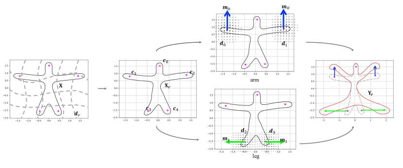
Figure S.4: Visualization of the Starman dataset simulation. The template shape $\mathbf{X}$ is in solid black, the control points $\{\mathbf{c}_{i}\}$ are the five points in magenta. The grey dashed lines represent the individual random deformation $\mathbf{d}_{r}$ to the template and those control points $\{\mathbf{c}_{i}\}$ , yielding an individualized template $\mathbf{X}_{r}$. The moving direction $\mathbf{m}_{0}$ controlling the two arms is in bold blue arrow. The moving direction $\mathbf{m}_{1}$ controlling the two legs is in bold green arrow. The velocity fields $\mathbf{d}_{0}$ and $\mathbf{d}_{1}$ control the upward/downward movement of two arms correspondingly. The velocity fields $\mathbf{d}_{2}$ and $\mathbf{d}_{3}$ controls the splits of two legs correspondingly. The individualized template shape $\mathbf{X}_{r}$ is deformed by $\mathbf{d}=\Sigma_{i}\mathbf{d}_{i}$ to $\mathbf{Y}_{r}$ (the red shape), representing a person moving their arms and legs. The covariates $\alpha$ and $\beta$ decide how much the arm is lifted and how much the legs are split.

S.2.2 ADNI Hippocampus

The ADNI hippocampus dataset consists of 1632 hippocampus segmentations from magnetic resonance (MR) images from the ADNI dataset, 80% (1297 shapes) of which are used for training and 20% (335 shapes) for testing. Each shape is associated with 4 covariates (age, sex, AD, education length). AD is a binary variable that represents whether a person has Alzheimer disease. AD=1 indicates a person has Alzheimer disease. Table S.5 shows the distribution of the number of observations across patients. Table S.6 shows the hippocampus shapes and the demographic information of an example patient. Table S.7 shows the shapes and demographic information at different age percentiles for the whole data set. We observe that the time span of our longitudinal data for each patient is far shorter than the time span across the entire dataset, indicating the challenge of capturing spatiotemporal dependencies over large time spans between shapes while accounting for individual differences between patients.

# observations	1	2	3	4	5	6
# patients	3	10	410	5	7	54

Table S.5: Number of patients for a given number of observations for the ADNI dataset. For example, the 1st column indicates that there are 3 patients who were only observed once.

# time	0	1	2	3	4	5
$\{\mathcal{S}^{t}\}$

	0	1	2	3	4	5
age	75.6	75.7	76.2	76.2	76.7	76.7
AD	No	No	No	No	No	No
sex	F	F	F	F	F	F
edu	20.0	20.0	20.0	20.0	20.0	20.0
m-vol	2.26	2.38	2.2	2.35	2.27	2.16

Table S.6: Visualization and demographic information of observations of a patient in the ADNI hippocampus dataset. Shapes are plotted with their covariates (age/yrs, AD, sex, edu(education length)/yrs) printed in the table. M-vol (measured volume) is the volume ($cm^{3}$) of the gold standard shapes based on the actual imaging.

P-	0	10	20	30	40	50	60	70	80	90	100
$\{\mathcal{S}^{t}\}$

	0	1	2	3	4	5	6	7	8	9	10
age	55.2	68.4	71.2	72.6	74.2	76.2	77.9	79.8	82.0	85.2	90.8
AD	No	No	Yes	No	No	No	Yes	Yes	No	No	No
sex	F	F	F	F	M	F	F	M	M	F	F
edu	18.0	16.0	16.0	15.0	18.0	18.0	17.0	20.0	16.0	7.0	15.0
m-vol	1.91	1.58	1.3	1.48	2.08	2.2	1.66	1.63	2.0	1.64	2.21

Table S.7: Visualization and demographic information of our ADNI Hippocampus 3D shape dataset. Shapes of $\{0,10,20,30,40,50,60,70,80,90,100\}$-th age percentiles are plotted with their covariates (age/yrs, AD, sex, edu(education length)/yrs) printed in the table. M-vol (measured volume) is the volume ($cm^{3}$) of the gold standard shapes based on the actual imaging.

S.2.3 Pediatric Airway

The airway shapes are extracted from computed tomography (CT) images. We use real CT images of children ranging in age from 1 month to $\sim$19 years old. Acquiring CT images is costly. Further, CT uses ionizing radiation which should be avoided, especially in children, due to cancer risks. Hence, it is difficult to acquire such CTs for many children. Instead, our data was acquired by serendipity from children who received CTs for reasons other than airway obstructions (e.g., because they had cancer). This also explains why it is difficult to acquire longitudinal data. E.g., one of our patients has 11 timepoints because a very sick child had to be scanned 11 times. Note that our data is very different from typical CV datasets which can be more readily acquired at scale or may even already exist based on internet photo collections. This is impossible for our task because image acquisition risks always have to be justified by patient benefits.

Our dataset includes 229 cross-sectional observations (where a patient was only imaged once) and 34 longitudinal observations. Each shape has 3 covariates (age, weight, sex) and 11 annotated anatomical landmarks. Errors in the shapes $\{\mathcal{S}^{k}\}$ may arise from image segmentation error, differences in head positioning, missing parts of the airway shapes due to incomplete image coverage, and dynamic airway deformations due to breathing. Table S.8 shows the distribution of the number of observations across patients. Most of the patients in the dataset only have one observation; only 22 patients have $\geq 3$ observation times. Table S.9 shows the airway shapes and the demographic information of an example patient. Table S.10 shows the shapes and demographic information at different age percentiles for the whole data set. Similar to the ADNI hippocampus dataset, the time span of the longitudinal data for each patient is far shorter than the time span across the entire dataset, which poses a significant shape analysis challenge for realistic medical shapes.

# observations	1	2	3	4	5	6	7	9	11
# patients	229	12	6	8	3	2	1	1	1

Table S.8: Number of patients for a given number of observations for the pediatric airway dataset. For example, the 1st column indicates that there are 229 patients who were only observed once.

#time	0	1	2	3	4	5	6	7	8
$\{\mathcal{S}^{t}\}$

#time	0	1	2	3	4	5	6	7	8
age	84.00	85.00	87.00	91.0	95.00	98.00	101.00	104.00	120.00
weight	20.40	20.40	21.00	21.9	22.80	22.90	23.50	24.90	28.50
sex	M	M	M	M	M	M	M	M	M
m-vol	30.07	32.18	48.95	33.8	44.87	42.29	28.42	40.92	61.36

Table S.9: Visualization and demographic information of observations of a patient in our 3D airway shape dataset. Shapes are plotted with their covariates (age/month, weight/kg, sex) printed in the table. M-vol (measured volume) is the volume ($cm^{3}$) of the gold standard shapes based on the actual imaging.

P-	0	10	20	30	40	50	60	70	80	90	100
$\{\mathcal{S}^{t}\}$

P-	0	10	20	30	40	50	60	70	80	90	100
age	1.00	23.00	55.00	71.00	89.00	111.00	129.00	161.00	179.00	199.00	233.00
weight	3.90	14.20	20.10	21.80	19.70	32.85	44.80	21.30	59.00	93.90	75.60
sex	M	M	F	F	M	M	M	F	F	F	M
m-vol	4.56	16.84	29.53	28.91	27.31	70.90	71.23	43.34	78.63	102.35	113.84

Table S.10: Visualization and demographic information of our 3D airway shape dataset. Shapes of $\{0,10,20,30,40,50,60,70,80,90,100\}$-th age percentiles are plotted with their covariates (age/month, weight/kg, sex) printed in the table. M-vol (measured volume) is the volume ($cm^{3}$) of the gold standard shapes based on the actual imaging.

Data Processing.

For the ADNI hippocampus dataset and the pediatric airway dataset, the shape meshes are extracted using Marching Cubes (Lorensen & Cline, 1987; Van der Walt et al., 2014) to obtain coordinates and normal vectors of on-surface points. The hippocapus shapes are rigidly aligned using the ICP algorithm (Arun et al., 1987). The airway shapes are rigidly aligned using the anatomical landmarks. The true vocal cords landmark is set to the origin. We follow the implementation in (Park et al., 2019) to sample 500,000 off-surface points. During training, it is important to preserve the scale information. We therefore scale all meshes with the same constant.

Appendix S.3 Experiments

Section S.3.1 describes implementation details Section S.3.2 describe the ablation study. Section S.3.3, Section S.3.4, and Section S.3.5 show additional experimental results for shape reconstruction, shape transfer, and disentangled shape evolution, respectively.

S.3.1 Implementation Details

Methods	DeepSDF	A-SDF	DIT	NDF	Ours
					Starman	ADNI Hippocampus	Pediatric Airway
#params	2.24M	1.98M	1.92M	0.34M	1.33M	2.26M	1.26M

Table S.11: Number of parameters of the different models.

Each subnetwork, including the template network $\mathcal{T}$ and the displacement networks $\{f_{i}\}$, are all parameterized with an $N_{l}$-layer MLP using $sine$ activations. We use $N_{l}$=8 for Starman and the ADNI hippocampus dataset; we use $N_{l}$=6 for the pediatric airway dataset. The network parameter initialization follows SIREN (Sitzmann et al., 2020). There are 256 hidden units in each layer. The architecture of $\mathcal{T}$ also follows SIREN (Sitzmann et al., 2020). The architecture of the $\{f_{i}\}$ follows DeepSDF (Park et al., 2019), in which a skip connection is used to concatenate the input of $(\mathbf{p},c_{i})$ to the input of the middle layer. We use a latent code $\mathbf{z}$ of dimension 256 ($L=256$). Table S.11 lists the number of model parameters.

For each training iteration, the number of points sampled from each shape is 750 ($N=750$), of which 500 are on-surface points ($N_{on}=500$) and the others are off-surface points ($N_{off}=250$). We train NAISR for 3000 epochs for airway dataset and 300 epochs for the ADNI hippocampus and Starman dataset using Adam (Kingma & Ba, 2014) with a learning rate $5e-5$ and batch size of 64. Also, we jointly optimize the latent code $\mathbf{z}$ with NAISR using Adam (Kingma & Ba, 2014) with a learning rate of $1e-3$.

During training, $\lambda_{1}=\lambda_{5}=\frac{10}{N}$; $\lambda_{2}=\frac{30}{N_{on}}$; $\lambda_{3}=\frac{10}{N_{on}}$, $\lambda_{4}=\frac{100}{N_{off}}$. For $\mathcal{L}_{lat}$, $\lambda_{6}=\frac{2}{L}$; $\sigma=0.01$ (following DeepSDF (Park et al., 2019)). During inference, the latent codes are optimized for $N_{t}$ iterations with a learning rate of $5e-3$. $N_{t}$ is set to 800 for the pediatric airway dataset; $N_{t}$ is set to 200 for the Starman and ADNI Hippocampus datasets.

Comparison Methods.

For shape reconstruction of unseen shapes, we compare our method on the test set with DeepSDF (Park et al., 2019) A-SDF (Mu et al., 2021) DIT (Zheng et al., 2021) and NDF (Sun et al., 2022). For shape transfer, we compare our method with A-SDF (Mu et al., 2021) because other comparison methods cannot model covariates as summarized in Table 1. The original implementations of the comparison methods did not produce satisfying reconstructions on our dataset. We therefore improved them by using our reconstruction losses and by using the SIREN backbone (Sitzmann et al., 2020) in DeepSDF (Park et al., 2019), A-SDF (Mu et al., 2021), and the template networks in DIT (Zheng et al., 2021) and NDF (Sun et al., 2022).

S.3.2 Ablation Study

We conduct an ablation study on the loss terms on the pediatric airway dataset. Airway shapes are more complicated than the Starman shapes and the hippocampi. Further, the number of shape samples is smallest among the three datasets. On this challenging dataset, we aim to observe the model robustness when using varying loss terms and our goal is to determine which loss terms are necessary and what suitable hyperparameter settings are.

Table S.12 and Table S.13 shows the shape reconstruction evaluation for different hyperparameter settings. We see that $\mathcal{L}_{Dirichlet}$ for off-surface points is the most important term. A lower $\lambda_{6}$ for the latent code regularizer $\mathcal{L}_{lat}$ yields better reconstruction results. Table S.14 shows an ablation study for shape transfer. We observe that the reconstruction losses $\mathcal{L}_{Dirichlet}$ and $\mathcal{L}_{Neumann}$ are important for shape transfer.

To sum up, removing any of the reconstruction losses ($\mathcal{L}_{Eikonal}$, $\mathcal{L}_{Dirichlet}$, $\mathcal{L}_{Neumann}$) hurts performance. A smaller $\lambda_{6}$ yields better reconstruction performance, but may hurt shape transfer performance.

			CD $\downarrow$		EMD $\downarrow$		HD $\downarrow$
Methods	variants	influenced term	$\mu$	M	$\mu$	M	$\mu$	M
Ours	$\lambda_{1}=\lambda_{5}=0$	$\mathcal{L}_{Eikonal}$	0.072	0.047	1.447	1.323	10.426	8.716
Ours	$\lambda_{4}=0$	$\mathcal{L}_{Dirichlet\_off\_surf}$	4.323	4.481	1.374	1.244	68.527	69.715
Ours	$\lambda_{3}=0$	$\mathcal{L}_{Neumann}$	0.081	0.051	1.449	1.307	10.269	8.546
Ours	$\lambda_{2}=0$	$\mathcal{L}_{Dirichlet\_on\_surf}$	0.124	0.077	1.912	1.682	10.803	8.916
Ours	$\lambda_{6}=0$	$\mathcal{L}_{lat}$	0.045	0.023	0.980	0.890	8.920	7.028
Ours	$\lambda_{6}*=0.01$	$\mathcal{L}_{lat}$	0.049	0.023	1.053	0.924	9.064	7.041
Ours	$\lambda_{6}*=0.1$	$\mathcal{L}_{lat}$	0.056	0.031	1.126	1.015	9.578	7.831
Ours	$\lambda_{6}*=1$	$\mathcal{L}_{lat}$	0.067	0.039	1.251	1.143	10.333	8.404
Ours	$\lambda_{6}*=10$	$\mathcal{L}_{lat}$	0.075	0.049	1.368	1.270	11.111	9.176
Ours	$\lambda_{6}*=100$	$\mathcal{L}_{lat}$	0.100	0.073	1.607	1.532	13.456	11.853

Table S.12: Ablation study: quantitative evaluation of shape reconstruction. Ours means covariates are not used as additional input to NAISR. The shadowed line is what we report in the main text.

			CD $\downarrow$		EMD $\downarrow$		HD $\downarrow$
Methods	variants	influenced term	$\mu$	M	$\mu$	M	$\mu$	M
Ours (c)	$\lambda_{1}=\lambda_{5}=0$	$\mathcal{L}_{Eikonal}$	0.097	0.052	1.559	1.344	11.178	9.426
Ours (c)	$\lambda_{4}=0$	$\mathcal{L}_{Dirichlet\_off\_surf}$	4.029	4.485	1.454	1.239	68.272	69.356
Ours (c)	$\lambda_{3}=0$	$\mathcal{L}_{Neumann}$	0.089	0.055	1.494	1.313	10.52	8.625
Ours (c)	$\lambda_{2}=0$	$\mathcal{L}_{Dirichlet\_on\_surf}$	0.151	0.09	2.058	1.756	11.354	9.569
Ours (c)	$\lambda_{6}=0$	$\mathcal{L}_{lat}$	0.041	0.019	0.936	0.834	8.677	7.335
Ours (c)	$\lambda_{6}*=0.01$	$\mathcal{L}_{lat}$	0.051	0.025	1.061	0.923	9.301	7.139
Ours (c)	$\lambda_{6}*=0.1$	$\mathcal{L}_{lat}$	0.061	0.031	1.154	1.043	9.875	8.151
Ours (c)	$\lambda_{6}*=1$	$\mathcal{L}_{lat}$	0.084	0.044	1.344	1.182	10.719	8.577
Ours (c)	$\lambda_{6}*=10$	$\mathcal{L}_{lat}$	0.109	0.058	1.554	1.336	11.933	9.705
Ours (c)	$\lambda_{6}*=100$	$\mathcal{L}_{lat}$	0.152	0.088	1.943	1.715	14.37	12.043

Table S.13: Ablation study: quantitative evaluation of shape reconstruction. Ours (c) means covariates are used as additional input to NAISR. $\mu$ indicates the mean value of the measurements; M indicates the median of the measurements. The shadowed line is what we report in the main text.

	ablations		Volume Difference $\downarrow$
			without covariates		with covariates
Methods	variarants	influenced term	$\mu$	M	$\mu$	M
Ours	$\lambda_{1}=\lambda_{5}=0$	$\mathcal{L}_{Eikonal}$	13.977	10.925	8.324	7.214
Ours	$\lambda_{4}=0$	$\mathcal{L}_{Dirichlet\_off\_surf}$	3736.527	3709.001	3693.514	3612.394
Ours	$\lambda_{3}=0$	$\mathcal{L}_{Neumann}$	24.717	24.877	26.094	25.311
Ours	$\lambda_{2}=0$	$\mathcal{L}_{Dirichlet\_on\_surf}$	55.579	57.766	64.845	63.442
Ours	$\lambda_{6}=0$	$\mathcal{L}_{lat}$	14.679	10.306	9.465	7.096
Ours	$\lambda_{6}*=0.01$	$\mathcal{L}_{lat}$	8.766	6.629	8.518	5.105
Ours	$\lambda_{6}*=0.1$	$\mathcal{L}_{lat}$	12.861	8.307	11.518	8.950
Ours	$\lambda_{6}*=1$	$\mathcal{L}_{lat}$	12.820	8.837	11.227	9.653
Ours	$\lambda_{6}*=10$	$\mathcal{L}_{lat}$	8.644	4.676	9.464	5.756
Ours	$\lambda_{6}*=100$	$\mathcal{L}_{lat}$	11.959	8.857	11.939	8.113

Table S.14: Ablation study: quantitative evaluation of shape transfer. $\mu$ indicates the mean value of the measurements; M indicates the median of the measurements. The shadowed line is what we report in the main text.

S.3.3 Shape Reconstruction

Figure S.5 and Figure S.6 visualize more reconstructed hippocampi and airway shapes respectively. We observe that NAISR produces detailed and complete reconstructions from noisy and incomplete observations.

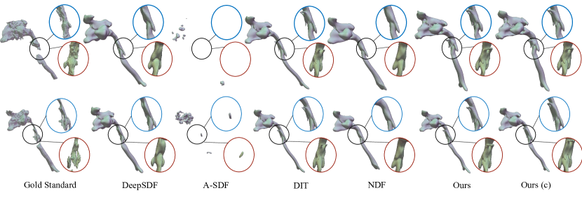
Figure S.5: Visualizations of airway shape reconstructions with different methods. The red and blue circles show the structure in the black circle from two different views. NAISR produces detailed and accurate reconstructions and imputes missing airway parts.

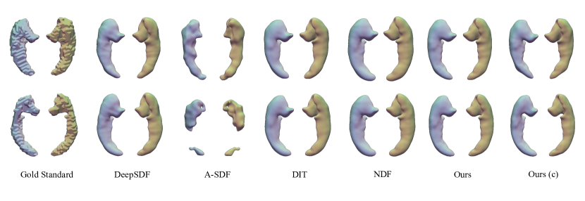
Figure S.6: Visualizations of hippocampus shape reconstructions with different methods. The red and blue circles show the structure in the black circle from two different views. All methods except for A-SDF are able to reconstruct well.

Each shape reconstruction method, except for A-SDF, successfully reconstructs airways and hippocampi. As discussed in Section 4.2, we suspect A-SDF overfits the training set by memorizing shapes with their covariates. We investigate this by evaluating shape reconstruction on the training set for A-SDF and NAISR as shown in Table S.15. From Table S.15, we can see that A-SDF overfits the training set.

	Training Set						Testing Set
	CD $\downarrow$		EMD $\downarrow$		HD $\downarrow$		CD $\downarrow$		EMD $\downarrow$		HD $\downarrow$
Methods	$\mu$	M	$\mu$	M	$\mu$	M	$\mu$	M	$\mu$	M	$\mu$	M
A-SDF	0.014	0.010	0.770	0.699	5.729	4.762	2.647	1.178	10.307	8.992	47.172	37.835
Ours	0.038	0.025	0.975	0.883	8.624	7.538	0.067	0.039	1.246	1.128	10.333	8.404

Table S.15: Comparison of NAISR and A-SDF on the training set. A-SDF performed well on the training set but failed on the testing set.

S.3.4 Shape Transfer

#time	0	1	2	3	4	5	6	7	8	9	10
$\{\mathcal{S}^{t}\}$

# time	0	1	2	3	4	5	6	7	8	9	10
age	154	155	157	159	163	164	167	170	194	227	233
weight	55.2	60.9	64.3	65.25	59.25	59.2	65.3	68	77.1	75.6	75.6
sex	M	M	M	M	M	M	M	M	M	M	M
p-vol	91.08	92.47	93.57	94.26	94.35	94.59	96.28	97.34	102.59	104.75	104.51
m-vol	86.33	82.66	63.23	90.65	98.11	84.35	94.14	127.45	98.81	100.17	113.84

Table S.16: Airway shape transfer without covariates as input for the patient shown in the main text. Blue: gold standard shapes; red: transferred shapes with NAISR. The table below lists the covariates (age/month, weight/kg, sex) for the shapes above. P-vol(predicted volume) is the volume ($cm^{3}$) of the transferred shape by NAISR with covariates following Eq. equation 9. M-vol (measured volume) is the volume ($cm^{3}$) of the shapes based on the actual imaging. The transferred shapes show similar growth trends in pediatric airways as shown in Table. 4.

Table S.16 shows the transferred airways using NAISR without covariates as input (following Equation 10). The predicted shapes from Equation 9 and Equation 10 look consistent in terms of appearance and development tendency. Table S.17 and Table S.18 show the transferred hippocampi. Due to the limited observation time span of patients in the ADNI hippocampus dataset, the volume stays almost constant.

# time	0	1	2	3	4
$\{\mathcal{S}^{t}\}$

# time	0	1	2	3	4
age	64.7	65.2	65.2	65.7	65.7
AD	No	No	No	No	No
sex	F	F	F	F	F
edu	14	14	14	14	14
p-vol	1.55	1.55	1.55	1.55	1.55
m-vol	1.49	1.56	1.55	1.45	1.55

Table S.17: Hippocampus shape transfer with covariates as input. Blue: gold standard shapes; red: transferred shapes with NAISR. The table below lists the covariates (age/yrs, AD, sex, edu(education length)/yrs for the shapes above. P-vol(predicted volume) is the volume ($cm^{3}$) of the transferred shape by NAISR with covariates following Equation 10. M-vol (measured volume) is the volume ($cm^{3}$) of the shapes based on the actual imaging. The transferred shapes stay almost the same in the one-year time period for this patient.

# time	0	1	2	3	4
$\{\mathcal{S}^{t}\}$

# time	0	1	2	3	4
age	64.7	65.2	65.2	65.7	65.7
AD	No	No	No	No	No
sex	F	F	F	F	F
edu	14	14	14	14	14
p-vol	1.6	1.6	1.6	1.6	1.6
m-vol	1.49	1.56	1.55	1.45	1.55

Table S.18: Hippocampus shape transfer without covariates as input. Blue: gold standard shapes; red: transferred shapes with NAISR. The table below lists the covariates (age/yrs, AD, sex, edu(education length)/yrs for the shapes above. P-vol(predicted volume) is the volume ($cm^{3}$) of the transferred shape by NAISR with covariates following Equation 9. M-vol (measured volume) is the volume ($cm^{3}$) of the shapes based on the actual imaging. The transferred shapes stay almost the same in the one-year period space for this patient.

S.3.5 Shape Disentanglement and Evolution

Fig. S.8 shows an example of airway shape extrapolation in covariate space for a patient in the testing set. Fig. S.9 shows an example of hippocampus shape extrapolation in covariate space for a patient in the testing set. We observe that in the range of observed covariates (inside the purple shade), shape extrapolation produces realistic-looking and reasonable growing/shrinking shapes in accordance with clinical expectations. Further, NAISR is able to extrapolate shapes outside this range, but the quality is lower than within the range of observed covariates.

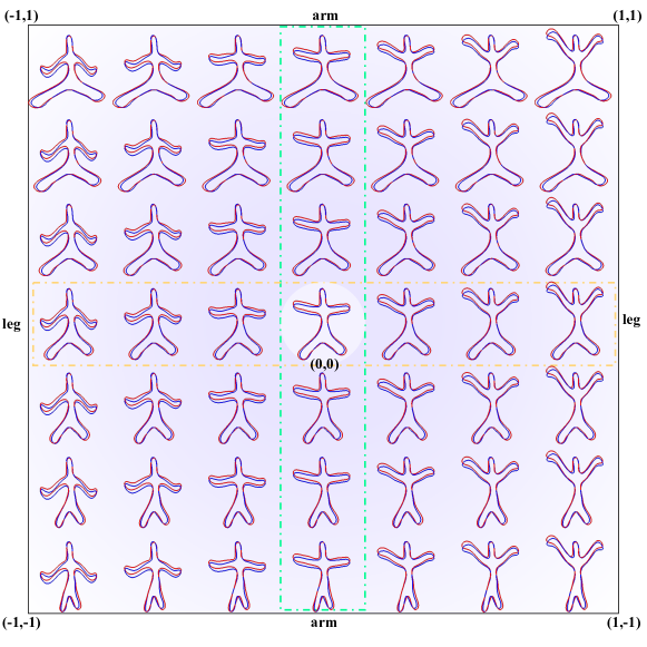
A-SDF, Starman

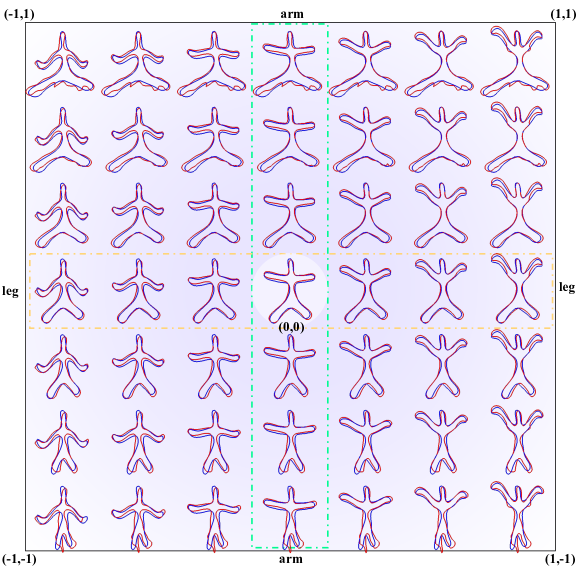
Ours, Starman

Figure S.7: Individualized Starman shape extrapolation in covariate space. The blue shapes are the groundtruth shapes and the red shapes are the reconstructions. The purple shadows over the space indicate the covariate range that the dataset covers. The latent code $\mathbf{z}$ is kept constant to create an individualized covariate shape space. The shapes in the green and yellow boxes are plotted with $\{\Phi_{i}\}$ (see Section 3.4), representing the disentangled shape evolutions along the arm and leg respectively. Shapes extrapolated from $\mathbf{z}_{i}$ look realistic and smooth across different covariates.

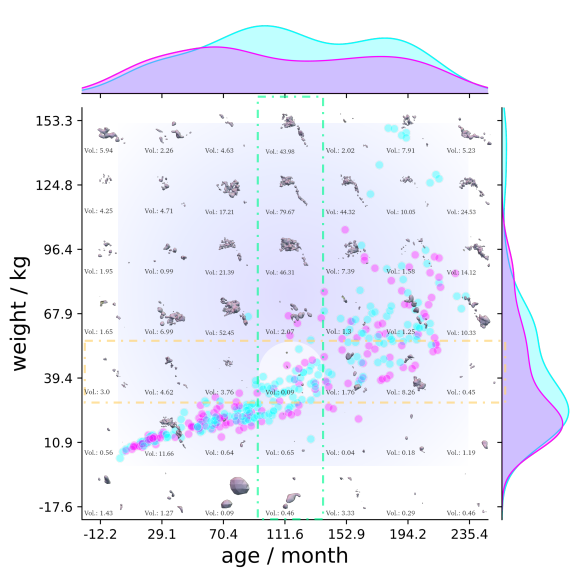
A-SDF, Pediatric Airway

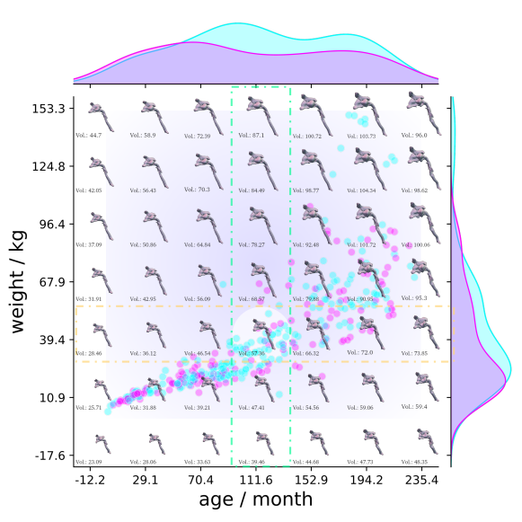
Ours, Pediatric Airway

Figure S.8: Individualized airway shape extrapolation in covariate space. Example shapes in the covariate space are visualized with their volumes ($cm^{3}$) below. Cyan points represent male and purple points female children in the dataset. The points represent the covariates of all children in the dataset. The purple shadows over the space indicate the covariate range that the dataset covers. The colored shades at the boundary represent the covariate distributions stratified by sex. The latent code $\mathbf{z}$ is kept constant to create an individualized covariate shape space. The shapes in the green and yellow boxes are plotted with $\{\Phi_{i}\}$ (see Section 3.4), representing the disentangled shape evolutions along weight and age respectively. Shapes extrapolated from $\mathbf{z}_{i}$ look realistic and smooth across different covariates.

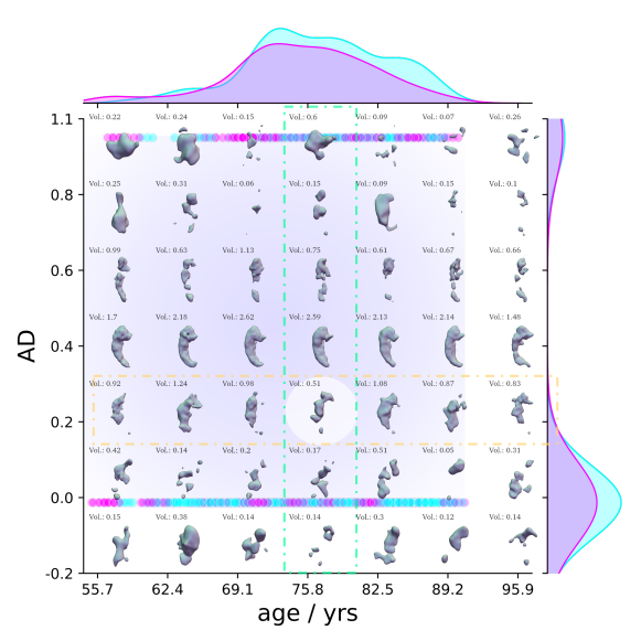
A-SDF, ADNI Hippocampus

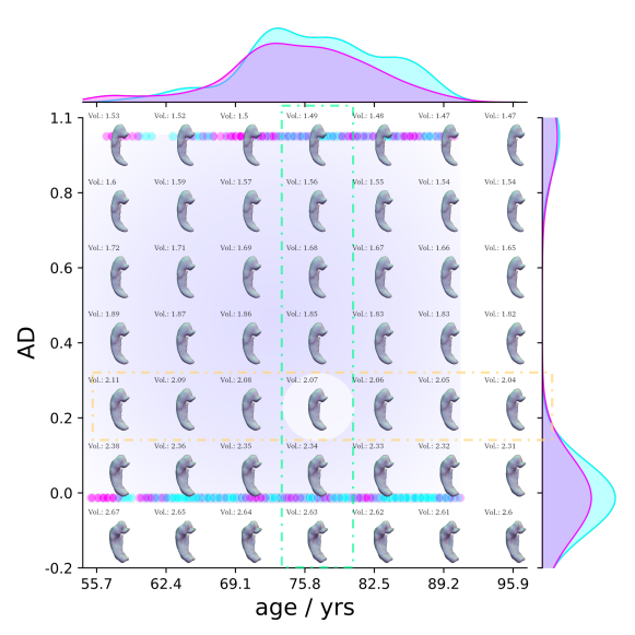
Ours, ADNI Hippocampus

Figure S.9: Individualized hippocampus shape extrapolation in covariate space. Example shapes in the covariate space are visualized with their volumes ($cm^{3}$) below. Cyan points represent male and purple points female patients in the dataset. The points represent the covariates of all patients in the dataset. The purple shadows over the space indicate the covariate range that the dataset covers. The colored shades at the boundary represent the covariate distributions stratified by sex. The latent code $\mathbf{z}$ is kept constant to create an individualized covariate shape space. The shapes in the green and yellow boxes are plotted with $\{\Phi_{i}\}$ (see Section 3.4), representing the disentangled shape evolutions along AD and age respectively. Shapes extrapolated from $\mathbf{z}_{i}$ look realistic and smooth across different covariates.

Appendix S.4 Limitations and Future Work

Invertible transformations are often desirable for shape correspondence. However, our approach cannot guarantee invertibility. Invertibility could be guaranteed by representing deformations via velocity fields instead of directly parameterizing deformation fields. However, velocity field parameterizations are costly as they require numerical integration. Hence, training such velocity field models for implicit shapes would consume more time and GPU resources. In future work, we will develop more efficient invertible representations, which will then assure that shape topology (wrt. the template shape) is preserved by construction. We also do not know the true effects of the covariates on the shapes. We can so far only indirectly assess our model by quantifying reconstruction, evolution, and transfer performance. In future work, we will include patients with airway abnormalities (e.g., with subglottic stenosis, an airway disease affecting airway geometry) in our analyses. This would allow us to further assess our NAISR model by exploring if our estimated model of normal airway shape can be used to detect airway abnormalities.

Appendix E Appendix

You may include other additional sections here.

References

- Achlioptas et al. (2018) Panos Achlioptas, Olga Diamanti, Ioannis Mitliagkas, and Leonidas Guibas. Learning representations and generative models for 3d point clouds. In International conference on machine learning, pp. 40–49. PMLR, 2018.
- Agarwal et al. (2020) Rishabh Agarwal, Nicholas Frosst, Xuezhou Zhang, Rich Caruana, and Geoffrey E Hinton. Neural additive models: Interpretable machine learning with neural nets. arXiv preprint arXiv:2004.13912, 2020.
- Arik & Pfister (2021) Sercan Ö Arik and Tomas Pfister. Tabnet: Attentive interpretable tabular learning. In Proceedings of the AAAI Conference on Artificial Intelligence, volume 35, pp. 6679–6687, 2021.
- Arun et al. (1987) K Somani Arun, Thomas S Huang, and Steven D Blostein. Least-squares fitting of two 3-d point sets. IEEE Transactions on pattern analysis and machine intelligence, (5):698–700, 1987.
- Bercea et al. (2022) Cosmin I Bercea, Benedikt Wiestler, Daniel Rueckert, and Shadi Albarqouni. Federated disentangled representation learning for unsupervised brain anomaly detection. Nature Machine Intelligence, 4(8):685–695, 2022.
- Berrevoets et al. (2021) Jeroen Berrevoets, Ahmed Alaa, Zhaozhi Qian, James Jordon, Alexander ES Gimson, and Mihaela Van Der Schaar. Learning queueing policies for organ transplantation allocation using interpretable counterfactual survival analysis. In International Conference on Machine Learning, pp. 792–802. PMLR, 2021.
- Bône et al. (2020) Alexandre Bône, Olivier Colliot, Stanley Durrleman, and Alzheimer’s Disease Neuroimaging Initiative. Learning the spatiotemporal variability in longitudinal shape data sets. International Journal of Computer Vision, 128(12):2873–2896, 2020.
- Chartsias et al. (2019) Agisilaos Chartsias, Thomas Joyce, Giorgos Papanastasiou, Scott Semple, Michelle Williams, David E Newby, Rohan Dharmakumar, and Sotirios A Tsaftaris. Disentangled representation learning in cardiac image analysis. Medical image analysis, 58:101535, 2019.
- Chen et al. (2022) Kan Chen, Qishuo Yin, and Qi Long. Covariate-balancing-aware interpretable deep learning models for treatment effect estimation. arXiv preprint arXiv:2203.03185, 2022.
- Chen et al. (2021) Xu Chen, Yufeng Zheng, Michael J Black, Otmar Hilliges, and Andreas Geiger. Snarf: Differentiable forward skinning for animating non-rigid neural implicit shapes. In Proceedings of the IEEE/CVF International Conference on Computer Vision, pp. 11594–11604, 2021.
- Chu et al. (2022) Jiebin Chu, Yaoyun Zhang, Fei Huang, Luo Si, Songfang Huang, and Zhengxing Huang. Disentangled representation for sequential treatment effect estimation. Computer Methods and Programs in Biomedicine, 226:107175, 2022.
- Crabbe et al. (2021) Jonathan Crabbe, Zhaozhi Qian, Fergus Imrie, and Mihaela van der Schaar. Explaining latent representations with a corpus of examples. In M. Ranzato, A. Beygelzimer, Y. Dauphin, P.S. Liang, and J. Wortman Vaughan (eds.), Advances in Neural Information Processing Systems, volume 34, pp. 12154–12166. Curran Associates, Inc., 2021. URL https://proceedings.neurips.cc/paper/2021/file/65658fde58ab3c2b6e5132a39fae7cb9-Paper.pdf.
- Dalca et al. (2019) Adrian Dalca, Marianne Rakic, John Guttag, and Mert Sabuncu. Learning conditional deformable templates with convolutional networks. Advances in neural information processing systems, 32, 2019.
- Deng et al. (2020) Boyang Deng, John P Lewis, Timothy Jeruzalski, Gerard Pons-Moll, Geoffrey Hinton, Mohammad Norouzi, and Andrea Tagliasacchi. Nasa neural articulated shape approximation. In Computer Vision–ECCV 2020: 16th European Conference, Glasgow, UK, August 23–28, 2020, Proceedings, Part VII 16, pp. 612–628. Springer, 2020.
- Deng et al. (2021) Yu Deng, Jiaolong Yang, and Xin Tong. Deformed implicit field: Modeling 3d shapes with learned dense correspondence. In Proceedings of the IEEE/CVF Conference on Computer Vision and Pattern Recognition, pp. 10286–10296, 2021.
- Ding et al. (2020) Zheng Ding, Yifan Xu, Weijian Xu, Gaurav Parmar, Yang Yang, Max Welling, and Zhuowen Tu. Guided variational autoencoder for disentanglement learning. In Proceedings of the IEEE/CVF conference on computer vision and pattern recognition, pp. 7920–7929, 2020.
- Gao et al. (2022) Jun Gao, Tianchang Shen, Zian Wang, Wenzheng Chen, Kangxue Yin, Daiqing Li, Or Litany, Zan Gojcic, and Sanja Fidler. Get3d: A generative model of high quality 3d textured shapes learned from images. In Advances In Neural Information Processing Systems, 2022.
- Gosche et al. (2002) KM Gosche, JA Mortimer, CD Smith, WR Markesbery, and DA Snowdon. Hippocampal volume as an index of Alzheimer neuropathology: findings from the nun study. Neurology, 58(10):1476–1482, 2002.
- Grattarola & Vandergheynst (2022) Daniele Grattarola and Pierre Vandergheynst. Generalised implicit neural representations. arXiv preprint arXiv:2205.15674, 2022.
- Gropp et al. (2020) Amos Gropp, Lior Yariv, Niv Haim, Matan Atzmon, and Yaron Lipman. Implicit geometric regularization for learning shapes. arXiv preprint arXiv:2002.10099, 2020.
- Groueix et al. (2018) Thibault Groueix, Matthew Fisher, Vladimir G Kim, Bryan C Russell, and Mathieu Aubry. A papier-mâché approach to learning 3d surface generation. In Proceedings of the IEEE conference on computer vision and pattern recognition, pp. 216–224, 2018.
- Hastie (2017) Trevor J Hastie. Generalized additive models. Routledge, 2017.
- Jack Jr et al. (2008) Clifford R Jack Jr, Matt A Bernstein, Nick C Fox, Paul Thompson, Gene Alexander, Danielle Harvey, Bret Borowski, Paula J Britson, Jennifer L. Whitwell, Chadwick Ward, et al. The Alzheimer’s disease neuroimaging initiative (ADNI): MRI methods. Journal of Magnetic Resonance Imaging: An Official Journal of the International Society for Magnetic Resonance in Medicine, 27(4):685–691, 2008.
- John et al. (2018) Vineet John, Lili Mou, Hareesh Bahuleyan, and Olga Vechtomova. Disentangled representation learning for non-parallel text style transfer. arXiv preprint arXiv:1808.04339, 2018.
- Jung & Oh (2021) Hyungsik Jung and Youngrock Oh. Towards better explanations of class activation mapping. In Proceedings of the IEEE/CVF International Conference on Computer Vision, pp. 1336–1344, 2021.
- Kingma & Ba (2014) Diederik P Kingma and Jimmy Ba. Adam: A method for stochastic optimization. arXiv preprint arXiv:1412.6980, 2014.
- Lorensen & Cline (1987) William E Lorensen and Harvey E Cline. Marching cubes: A high resolution 3d surface construction algorithm. ACM siggraph computer graphics, 21(4):163–169, 1987.
- Luscan et al. (2020) Romain Luscan, Nicolas Leboulanger, Pierre Fayoux, Gaspard Kerner, Kahina Belhous, Vincent Couloigner, Erea-Noël Garabedian, François Simon, Françoise Denoyelle, and Briac Thierry. Developmental changes of upper airway dimensions in children. Pediatric Anesthesia, 30(4):435–445, 2020.
- Mescheder et al. (2019) Lars Mescheder, Michael Oechsle, Michael Niemeyer, Sebastian Nowozin, and Andreas Geiger. Occupancy networks: Learning 3d reconstruction in function space. In Proceedings of the IEEE/CVF conference on computer vision and pattern recognition, pp. 4460–4470, 2019.
- Moraffah et al. (2020) Raha Moraffah, Mansooreh Karami, Ruocheng Guo, Adrienne Raglin, and Huan Liu. Causal interpretability for machine learning-problems, methods and evaluation. ACM SIGKDD Explorations Newsletter, 22(1):18–33, 2020.
- Mu et al. (2021) Jiteng Mu, Weichao Qiu, Adam Kortylewski, Alan Yuille, Nuno Vasconcelos, and Xiaolong Wang. A-sdf: Learning disentangled signed distance functions for articulated shape representation. In Proceedings of the IEEE/CVF International Conference on Computer Vision, pp. 13001–13011, 2021.
- Niemeyer et al. (2019) Michael Niemeyer, Lars Mescheder, Michael Oechsle, and Andreas Geiger. Occupancy flow: 4d reconstruction by learning particle dynamics. In Proceedings of the IEEE/CVF international conference on computer vision, pp. 5379–5389, 2019.
- Novello et al. (2022) Tiago Novello, Guilherme Schardong, Luiz Schirmer, Vinícius da Silva, Hélio Lopes, and Luiz Velho. Exploring differential geometry in neural implicits. Computers & Graphics, 108:49–60, 2022.
- Osher & Fedkiw (2005) Stanley Osher and Ronald P Fedkiw. Level set methods and dynamic implicit surfaces, volume 1. Springer New York, 2005.
- Palafox et al. (2021) Pablo Palafox, Aljaž Božič, Justus Thies, Matthias Nießner, and Angela Dai. Npms: Neural parametric models for 3d deformable shapes. In Proceedings of the IEEE/CVF International Conference on Computer Vision, pp. 12695–12705, 2021.
- Palafox et al. (2022) Pablo Palafox, Nikolaos Sarafianos, Tony Tung, and Angela Dai. Spams: Structured implicit parametric models. In Proceedings of the IEEE/CVF Conference on Computer Vision and Pattern Recognition, pp. 12851–12860, 2022.
- Park et al. (2019) Jeong Joon Park, Peter Florence, Julian Straub, Richard Newcombe, and Steven Lovegrove. Deepsdf: Learning continuous signed distance functions for shape representation. In Proceedings of the IEEE/CVF conference on computer vision and pattern recognition, pp. 165–174, 2019.
- Petersen et al. (2010) Ronald Carl Petersen, Paul S Aisen, Laurel A Beckett, Michael C Donohue, Anthony Collins Gamst, Danielle J Harvey, Clifford R Jack, William J Jagust, Leslie M Shaw, Arthur W Toga, et al. Alzheimer’s disease neuroimaging initiative (adni): clinical characterization. Neurology, 74(3):201–209, 2010.
- Phongthawee et al. (2022) Pakkapon Phongthawee, Suttisak Wizadwongsa, Jiraphon Yenphraphai, and Supasorn Suwajanakorn. Nex360: Real-time all-around view synthesis with neural basis expansion. IEEE Transactions on Pattern Analysis and Machine Intelligence, 2022.
- Ribeiro et al. (2016) Marco Tulio Ribeiro, Sameer Singh, and Carlos Guestrin. "Why should i trust you?" Explaining the predictions of any classifier. In Proceedings of the 22nd ACM SIGKDD international conference on knowledge discovery and data mining, pp. 1135–1144, 2016.
- Sethian (1999) James Albert Sethian. Level set methods and fast marching methods: evolving interfaces in computational geometry, fluid mechanics, computer vision, and materials science, volume 3. Cambridge university press, 1999.
- Shen et al. (2021) Tianchang Shen, Jun Gao, Kangxue Yin, Ming-Yu Liu, and Sanja Fidler. Deep marching tetrahedra: a hybrid representation for high-resolution 3d shape synthesis. Advances in Neural Information Processing Systems, 34:6087–6101, 2021.
- Shoshan et al. (2021) Alon Shoshan, Nadav Bhonker, Igor Kviatkovsky, and Gerard Medioni. GAN-control: Explicitly controllable GANs. In Proceedings of the IEEE/CVF international conference on computer vision, pp. 14083–14093, 2021.
- Sitzmann et al. (2020) Vincent Sitzmann, Julien Martel, Alexander Bergman, David Lindell, and Gordon Wetzstein. Implicit neural representations with periodic activation functions. Advances in Neural Information Processing Systems, 33:7462–7473, 2020.
- Stammer et al. (2022) Wolfgang Stammer, Marius Memmel, Patrick Schramowski, and Kristian Kersting. Interactive disentanglement: Learning concepts by interacting with their prototype representations. In Proceedings of the IEEE/CVF Conference on Computer Vision and Pattern Recognition, pp. 10317–10328, 2022.
- Sun et al. (2022) Shanlin Sun, Kun Han, Deying Kong, Hao Tang, Xiangyi Yan, and Xiaohui Xie. Topology-preserving shape reconstruction and registration via neural diffeomorphic flow. In Proceedings of the IEEE/CVF Conference on Computer Vision and Pattern Recognition, pp. 20845–20855, 2022.
- Tewari et al. (2022) Ayush Tewari, Xingang Pan, Ohad Fried, Maneesh Agrawala, Christian Theobalt, et al. Disentangled3d: Learning a 3d generative model with disentangled geometry and appearance from monocular images. In Proceedings of the IEEE/CVF Conference on Computer Vision and Pattern Recognition, pp. 1516–1525, 2022.
- Thiagarajan et al. (2020) Jayaraman J Thiagarajan, Prasanna Sattigeri, Deepta Rajan, and Bindya Venkatesh. Calibrating healthcare AI: Towards reliable and interpretable deep predictive models. arXiv preprint arXiv:2004.14480, 2020.
- Tretschk et al. (2020) Edgar Tretschk, Ayush Tewari, Vladislav Golyanik, Michael Zollhöfer, Carsten Stoll, and Christian Theobalt. Patchnets: Patch-based generalizable deep implicit 3d shape representations. In Computer Vision–ECCV 2020: 16th European Conference, Glasgow, UK, August 23–28, 2020, Proceedings, Part XVI 16, pp. 293–309. Springer, 2020.
- Van der Walt et al. (2014) Stefan Van der Walt, Johannes L Schönberger, Juan Nunez-Iglesias, François Boulogne, Joshua D Warner, Neil Yager, Emmanuelle Gouillart, and Tony Yu. scikit-image: image processing in python. PeerJ, 2:e453, 2014.
- Wei et al. (2022) Fangyin Wei, Rohan Chabra, Lingni Ma, Christoph Lassner, Michael Zollhoefer, Szymon Rusinkiewicz, Chris Sweeney, Richard Newcombe, and Mira Slavcheva. Self-supervised neural articulated shape and appearance models. In Proceedings IEEE/CVF Conference on Computer Vision and Pattern Recognition (CVPR), 2022.
- Wen et al. (2019) Chao Wen, Yinda Zhang, Zhuwen Li, and Yanwei Fu. Pixel2mesh++: Multi-view 3d mesh generation via deformation. In Proceedings of the IEEE/CVF international conference on computer vision, pp. 1042–1051, 2019.
- Wen et al. (2022) Xin Wen, Junsheng Zhou, Yu-Shen Liu, Hua Su, Zhen Dong, and Zhizhong Han. 3d shape reconstruction from 2d images with disentangled attribute flow. In Proceedings of the IEEE/CVF conference on computer vision and pattern recognition, pp. 3803–3813, 2022.
- Wolterink et al. (2022) Jelmer M Wolterink, Jesse C Zwienenberg, and Christoph Brune. Implicit neural representations for deformable image registration. In International Conference on Medical Imaging with Deep Learning, pp. 1349–1359. PMLR, 2022.
- Woo et al. (2018) Sanghyun Woo, Jongchan Park, Joon-Young Lee, and In So Kweon. Cbam: Convolutional block attention module. In Proceedings of the European conference on computer vision (ECCV), pp. 3–19, 2018.
- Wu et al. (2016) Jiajun Wu, Chengkai Zhang, Tianfan Xue, Bill Freeman, and Josh Tenenbaum. Learning a probabilistic latent space of object shapes via 3d generative-adversarial modeling. Advances in neural information processing systems, 29, 2016.
- Wu et al. (2018) Jiajun Wu, Chengkai Zhang, Xiuming Zhang, Zhoutong Zhang, William T Freeman, and Joshua B Tenenbaum. Learning shape priors for single-view 3d completion and reconstruction. In Proceedings of the European Conference on Computer Vision (ECCV), pp. 646–662, 2018.
- Wu et al. (2015) Zhirong Wu, Shuran Song, Aditya Khosla, Fisher Yu, Linguang Zhang, Xiaoou Tang, and Jianxiong Xiao. 3d shapenets: A deep representation for volumetric shapes. In Proceedings of the IEEE conference on computer vision and pattern recognition, pp. 1912–1920, 2015.
- Xu et al. (2021) Mutian Xu, Junhao Zhang, Zhipeng Zhou, Mingye Xu, Xiaojuan Qi, and Yu Qiao. Learning geometry-disentangled representation for complementary understanding of 3d object point cloud. In Proceedings of the AAAI Conference on Artificial Intelligence, volume 35, pp. 3056–3064, 2021.
- Yang et al. (2022a) Bangbang Yang, Chong Bao, Junyi Zeng, Hujun Bao, Yinda Zhang, Zhaopeng Cui, and Guofeng Zhang. Neumesh: Learning disentangled neural mesh-based implicit field for geometry and texture editing. In Computer Vision–ECCV 2022: 17th European Conference, Tel Aviv, Israel, October 23–27, 2022, Proceedings, Part XVI, pp. 597–614. Springer, 2022a.
- Yang et al. (2021) Guandao Yang, Serge Belongie, Bharath Hariharan, and Vladlen Koltun. Geometry processing with neural fields. Advances in Neural Information Processing Systems, 34:22483–22497, 2021.
- Yang et al. (2022b) Jiancheng Yang, Udaranga Wickramasinghe, Bingbing Ni, and Pascal Fua. ImplicitAtlas: learning deformable shape templates in medical imaging. In Proceedings of the IEEE/CVF Conference on Computer Vision and Pattern Recognition, pp. 15861–15871, 2022b.
- Yang et al. (2020) Jie Yang, Kaichun Mo, Yu-Kun Lai, Leonidas J Guibas, and Lin Gao. Dsm-net: Disentangled structured mesh net for controllable generation of fine geometry. arXiv preprint arXiv:2008.05440, 2(3), 2020.
- Yang et al. (2018) Yaoqing Yang, Chen Feng, Yiru Shen, and Dong Tian. Foldingnet: Point cloud auto-encoder via deep grid deformation. In Proceedings of the IEEE conference on computer vision and pattern recognition, pp. 206–215, 2018.
- Zamorski et al. (2020) Maciej Zamorski, Maciej Zięba, Piotr Klukowski, Rafał Nowak, Karol Kurach, Wojciech Stokowiec, and Tomasz Trzciński. Adversarial autoencoders for compact representations of 3d point clouds. Computer Vision and Image Understanding, 193:102921, 2020.
- Zhang et al. (2018a) Xiuming Zhang, Zhoutong Zhang, Chengkai Zhang, Josh Tenenbaum, Bill Freeman, and Jiajun Wu. Learning to reconstruct shapes from unseen classes. Advances in neural information processing systems, 31, 2018a.
- Zhang et al. (2018b) Yuting Zhang, Yijie Guo, Yixin Jin, Yijun Luo, Zhiyuan He, and Honglak Lee. Unsupervised discovery of object landmarks as structural representations. In Proceedings of the IEEE Conference on Computer Vision and Pattern Recognition, pp. 2694–2703, 2018b.
- Zheng et al. (2021) Zerong Zheng, Tao Yu, Qionghai Dai, and Yebin Liu. Deep implicit templates for 3d shape representation. In Proceedings of the IEEE/CVF Conference on Computer Vision and Pattern Recognition, pp. 1429–1439, 2021.
- Zhou et al. (2016) Bolei Zhou, Aditya Khosla, Agata Lapedriza, Aude Oliva, and Antonio Torralba. Learning deep features for discriminative localization. In Computer Vision and Pattern Recognition, 2016.
- Zhu et al. (2019) Hao Zhu, Xinxin Zuo, Sen Wang, Xun Cao, and Ruigang Yang. Detailed human shape estimation from a single image by hierarchical mesh deformation. In Proceedings of the IEEE/CVF conference on computer vision and pattern recognition, pp. 4491–4500, 2019.

References

- Achlioptas et al. (2018) Panos Achlioptas, Olga Diamanti, Ioannis Mitliagkas, and Leonidas Guibas. Learning representations and generative models for 3d point clouds. In International conference on machine learning, pp. 40–49. PMLR, 2018.
- Agarwal et al. (2020) Rishabh Agarwal, Nicholas Frosst, Xuezhou Zhang, Rich Caruana, and Geoffrey E Hinton. Neural additive models: Interpretable machine learning with neural nets. arXiv preprint arXiv:2004.13912, 2020.
- Arik & Pfister (2021) Sercan Ö Arik and Tomas Pfister. Tabnet: Attentive interpretable tabular learning. In Proceedings of the AAAI Conference on Artificial Intelligence, volume 35, pp. 6679–6687, 2021.
- Arun et al. (1987) K Somani Arun, Thomas S Huang, and Steven D Blostein. Least-squares fitting of two 3-d point sets. IEEE Transactions on pattern analysis and machine intelligence, (5):698–700, 1987.
- Bercea et al. (2022) Cosmin I Bercea, Benedikt Wiestler, Daniel Rueckert, and Shadi Albarqouni. Federated disentangled representation learning for unsupervised brain anomaly detection. Nature Machine Intelligence, 4(8):685–695, 2022.
- Berrevoets et al. (2021) Jeroen Berrevoets, Ahmed Alaa, Zhaozhi Qian, James Jordon, Alexander ES Gimson, and Mihaela Van Der Schaar. Learning queueing policies for organ transplantation allocation using interpretable counterfactual survival analysis. In International Conference on Machine Learning, pp. 792–802. PMLR, 2021.
- Bône et al. (2020) Alexandre Bône, Olivier Colliot, Stanley Durrleman, and Alzheimer’s Disease Neuroimaging Initiative. Learning the spatiotemporal variability in longitudinal shape data sets. International Journal of Computer Vision, 128(12):2873–2896, 2020.
- Chartsias et al. (2019) Agisilaos Chartsias, Thomas Joyce, Giorgos Papanastasiou, Scott Semple, Michelle Williams, David E Newby, Rohan Dharmakumar, and Sotirios A Tsaftaris. Disentangled representation learning in cardiac image analysis. Medical image analysis, 58:101535, 2019.
- Chen et al. (2022) Kan Chen, Qishuo Yin, and Qi Long. Covariate-balancing-aware interpretable deep learning models for treatment effect estimation. arXiv preprint arXiv:2203.03185, 2022.
- Chen et al. (2021) Xu Chen, Yufeng Zheng, Michael J Black, Otmar Hilliges, and Andreas Geiger. Snarf: Differentiable forward skinning for animating non-rigid neural implicit shapes. In Proceedings of the IEEE/CVF International Conference on Computer Vision, pp. 11594–11604, 2021.
- Chu et al. (2022) Jiebin Chu, Yaoyun Zhang, Fei Huang, Luo Si, Songfang Huang, and Zhengxing Huang. Disentangled representation for sequential treatment effect estimation. Computer Methods and Programs in Biomedicine, 226:107175, 2022.
- Crabbe et al. (2021) Jonathan Crabbe, Zhaozhi Qian, Fergus Imrie, and Mihaela van der Schaar. Explaining latent representations with a corpus of examples. In M. Ranzato, A. Beygelzimer, Y. Dauphin, P.S. Liang, and J. Wortman Vaughan (eds.), Advances in Neural Information Processing Systems, volume 34, pp. 12154–12166. Curran Associates, Inc., 2021. URL https://proceedings.neurips.cc/paper/2021/file/65658fde58ab3c2b6e5132a39fae7cb9-Paper.pdf.
- Dalca et al. (2019) Adrian Dalca, Marianne Rakic, John Guttag, and Mert Sabuncu. Learning conditional deformable templates with convolutional networks. Advances in neural information processing systems, 32, 2019.
- Deng et al. (2020) Boyang Deng, John P Lewis, Timothy Jeruzalski, Gerard Pons-Moll, Geoffrey Hinton, Mohammad Norouzi, and Andrea Tagliasacchi. Nasa neural articulated shape approximation. In Computer Vision–ECCV 2020: 16th European Conference, Glasgow, UK, August 23–28, 2020, Proceedings, Part VII 16, pp. 612–628. Springer, 2020.
- Deng et al. (2021) Yu Deng, Jiaolong Yang, and Xin Tong. Deformed implicit field: Modeling 3d shapes with learned dense correspondence. In Proceedings of the IEEE/CVF Conference on Computer Vision and Pattern Recognition, pp. 10286–10296, 2021.
- Ding et al. (2020) Zheng Ding, Yifan Xu, Weijian Xu, Gaurav Parmar, Yang Yang, Max Welling, and Zhuowen Tu. Guided variational autoencoder for disentanglement learning. In Proceedings of the IEEE/CVF conference on computer vision and pattern recognition, pp. 7920–7929, 2020.
- Gao et al. (2022) Jun Gao, Tianchang Shen, Zian Wang, Wenzheng Chen, Kangxue Yin, Daiqing Li, Or Litany, Zan Gojcic, and Sanja Fidler. Get3d: A generative model of high quality 3d textured shapes learned from images. In Advances In Neural Information Processing Systems, 2022.
- Gosche et al. (2002) KM Gosche, JA Mortimer, CD Smith, WR Markesbery, and DA Snowdon. Hippocampal volume as an index of Alzheimer neuropathology: findings from the nun study. Neurology, 58(10):1476–1482, 2002.
- Grattarola & Vandergheynst (2022) Daniele Grattarola and Pierre Vandergheynst. Generalised implicit neural representations. arXiv preprint arXiv:2205.15674, 2022.
- Gropp et al. (2020) Amos Gropp, Lior Yariv, Niv Haim, Matan Atzmon, and Yaron Lipman. Implicit geometric regularization for learning shapes. arXiv preprint arXiv:2002.10099, 2020.
- Groueix et al. (2018) Thibault Groueix, Matthew Fisher, Vladimir G Kim, Bryan C Russell, and Mathieu Aubry. A papier-mâché approach to learning 3d surface generation. In Proceedings of the IEEE conference on computer vision and pattern recognition, pp. 216–224, 2018.
- Hastie (2017) Trevor J Hastie. Generalized additive models. Routledge, 2017.
- Jack Jr et al. (2008) Clifford R Jack Jr, Matt A Bernstein, Nick C Fox, Paul Thompson, Gene Alexander, Danielle Harvey, Bret Borowski, Paula J Britson, Jennifer L. Whitwell, Chadwick Ward, et al. The Alzheimer’s disease neuroimaging initiative (ADNI): MRI methods. Journal of Magnetic Resonance Imaging: An Official Journal of the International Society for Magnetic Resonance in Medicine, 27(4):685–691, 2008.
- John et al. (2018) Vineet John, Lili Mou, Hareesh Bahuleyan, and Olga Vechtomova. Disentangled representation learning for non-parallel text style transfer. arXiv preprint arXiv:1808.04339, 2018.
- Jung & Oh (2021) Hyungsik Jung and Youngrock Oh. Towards better explanations of class activation mapping. In Proceedings of the IEEE/CVF International Conference on Computer Vision, pp. 1336–1344, 2021.
- Kingma & Ba (2014) Diederik P Kingma and Jimmy Ba. Adam: A method for stochastic optimization. arXiv preprint arXiv:1412.6980, 2014.
- Lorensen & Cline (1987) William E Lorensen and Harvey E Cline. Marching cubes: A high resolution 3d surface construction algorithm. ACM siggraph computer graphics, 21(4):163–169, 1987.
- Luscan et al. (2020) Romain Luscan, Nicolas Leboulanger, Pierre Fayoux, Gaspard Kerner, Kahina Belhous, Vincent Couloigner, Erea-Noël Garabedian, François Simon, Françoise Denoyelle, and Briac Thierry. Developmental changes of upper airway dimensions in children. Pediatric Anesthesia, 30(4):435–445, 2020.
- Mescheder et al. (2019) Lars Mescheder, Michael Oechsle, Michael Niemeyer, Sebastian Nowozin, and Andreas Geiger. Occupancy networks: Learning 3d reconstruction in function space. In Proceedings of the IEEE/CVF conference on computer vision and pattern recognition, pp. 4460–4470, 2019.
- Moraffah et al. (2020) Raha Moraffah, Mansooreh Karami, Ruocheng Guo, Adrienne Raglin, and Huan Liu. Causal interpretability for machine learning-problems, methods and evaluation. ACM SIGKDD Explorations Newsletter, 22(1):18–33, 2020.
- Mu et al. (2021) Jiteng Mu, Weichao Qiu, Adam Kortylewski, Alan Yuille, Nuno Vasconcelos, and Xiaolong Wang. A-sdf: Learning disentangled signed distance functions for articulated shape representation. In Proceedings of the IEEE/CVF International Conference on Computer Vision, pp. 13001–13011, 2021.
- Niemeyer et al. (2019) Michael Niemeyer, Lars Mescheder, Michael Oechsle, and Andreas Geiger. Occupancy flow: 4d reconstruction by learning particle dynamics. In Proceedings of the IEEE/CVF international conference on computer vision, pp. 5379–5389, 2019.
- Novello et al. (2022) Tiago Novello, Guilherme Schardong, Luiz Schirmer, Vinícius da Silva, Hélio Lopes, and Luiz Velho. Exploring differential geometry in neural implicits. Computers & Graphics, 108:49–60, 2022.
- Osher & Fedkiw (2005) Stanley Osher and Ronald P Fedkiw. Level set methods and dynamic implicit surfaces, volume 1. Springer New York, 2005.
- Palafox et al. (2021) Pablo Palafox, Aljaž Božič, Justus Thies, Matthias Nießner, and Angela Dai. Npms: Neural parametric models for 3d deformable shapes. In Proceedings of the IEEE/CVF International Conference on Computer Vision, pp. 12695–12705, 2021.
- Palafox et al. (2022) Pablo Palafox, Nikolaos Sarafianos, Tony Tung, and Angela Dai. Spams: Structured implicit parametric models. In Proceedings of the IEEE/CVF Conference on Computer Vision and Pattern Recognition, pp. 12851–12860, 2022.
- Park et al. (2019) Jeong Joon Park, Peter Florence, Julian Straub, Richard Newcombe, and Steven Lovegrove. Deepsdf: Learning continuous signed distance functions for shape representation. In Proceedings of the IEEE/CVF conference on computer vision and pattern recognition, pp. 165–174, 2019.
- Petersen et al. (2010) Ronald Carl Petersen, Paul S Aisen, Laurel A Beckett, Michael C Donohue, Anthony Collins Gamst, Danielle J Harvey, Clifford R Jack, William J Jagust, Leslie M Shaw, Arthur W Toga, et al. Alzheimer’s disease neuroimaging initiative (adni): clinical characterization. Neurology, 74(3):201–209, 2010.
- Phongthawee et al. (2022) Pakkapon Phongthawee, Suttisak Wizadwongsa, Jiraphon Yenphraphai, and Supasorn Suwajanakorn. Nex360: Real-time all-around view synthesis with neural basis expansion. IEEE Transactions on Pattern Analysis and Machine Intelligence, 2022.
- Ribeiro et al. (2016) Marco Tulio Ribeiro, Sameer Singh, and Carlos Guestrin. "Why should i trust you?" Explaining the predictions of any classifier. In Proceedings of the 22nd ACM SIGKDD international conference on knowledge discovery and data mining, pp. 1135–1144, 2016.
- Sethian (1999) James Albert Sethian. Level set methods and fast marching methods: evolving interfaces in computational geometry, fluid mechanics, computer vision, and materials science, volume 3. Cambridge university press, 1999.
- Shen et al. (2021) Tianchang Shen, Jun Gao, Kangxue Yin, Ming-Yu Liu, and Sanja Fidler. Deep marching tetrahedra: a hybrid representation for high-resolution 3d shape synthesis. Advances in Neural Information Processing Systems, 34:6087–6101, 2021.
- Shoshan et al. (2021) Alon Shoshan, Nadav Bhonker, Igor Kviatkovsky, and Gerard Medioni. GAN-control: Explicitly controllable GANs. In Proceedings of the IEEE/CVF international conference on computer vision, pp. 14083–14093, 2021.
- Sitzmann et al. (2020) Vincent Sitzmann, Julien Martel, Alexander Bergman, David Lindell, and Gordon Wetzstein. Implicit neural representations with periodic activation functions. Advances in Neural Information Processing Systems, 33:7462–7473, 2020.
- Stammer et al. (2022) Wolfgang Stammer, Marius Memmel, Patrick Schramowski, and Kristian Kersting. Interactive disentanglement: Learning concepts by interacting with their prototype representations. In Proceedings of the IEEE/CVF Conference on Computer Vision and Pattern Recognition, pp. 10317–10328, 2022.
- Sun et al. (2022) Shanlin Sun, Kun Han, Deying Kong, Hao Tang, Xiangyi Yan, and Xiaohui Xie. Topology-preserving shape reconstruction and registration via neural diffeomorphic flow. In Proceedings of the IEEE/CVF Conference on Computer Vision and Pattern Recognition, pp. 20845–20855, 2022.
- Tewari et al. (2022) Ayush Tewari, Xingang Pan, Ohad Fried, Maneesh Agrawala, Christian Theobalt, et al. Disentangled3d: Learning a 3d generative model with disentangled geometry and appearance from monocular images. In Proceedings of the IEEE/CVF Conference on Computer Vision and Pattern Recognition, pp. 1516–1525, 2022.
- Thiagarajan et al. (2020) Jayaraman J Thiagarajan, Prasanna Sattigeri, Deepta Rajan, and Bindya Venkatesh. Calibrating healthcare AI: Towards reliable and interpretable deep predictive models. arXiv preprint arXiv:2004.14480, 2020.
- Tretschk et al. (2020) Edgar Tretschk, Ayush Tewari, Vladislav Golyanik, Michael Zollhöfer, Carsten Stoll, and Christian Theobalt. Patchnets: Patch-based generalizable deep implicit 3d shape representations. In Computer Vision–ECCV 2020: 16th European Conference, Glasgow, UK, August 23–28, 2020, Proceedings, Part XVI 16, pp. 293–309. Springer, 2020.
- Van der Walt et al. (2014) Stefan Van der Walt, Johannes L Schönberger, Juan Nunez-Iglesias, François Boulogne, Joshua D Warner, Neil Yager, Emmanuelle Gouillart, and Tony Yu. scikit-image: image processing in python. PeerJ, 2:e453, 2014.
- Wei et al. (2022) Fangyin Wei, Rohan Chabra, Lingni Ma, Christoph Lassner, Michael Zollhoefer, Szymon Rusinkiewicz, Chris Sweeney, Richard Newcombe, and Mira Slavcheva. Self-supervised neural articulated shape and appearance models. In Proceedings IEEE/CVF Conference on Computer Vision and Pattern Recognition (CVPR), 2022.
- Wen et al. (2019) Chao Wen, Yinda Zhang, Zhuwen Li, and Yanwei Fu. Pixel2mesh++: Multi-view 3d mesh generation via deformation. In Proceedings of the IEEE/CVF international conference on computer vision, pp. 1042–1051, 2019.
- Wen et al. (2022) Xin Wen, Junsheng Zhou, Yu-Shen Liu, Hua Su, Zhen Dong, and Zhizhong Han. 3d shape reconstruction from 2d images with disentangled attribute flow. In Proceedings of the IEEE/CVF conference on computer vision and pattern recognition, pp. 3803–3813, 2022.
- Wolterink et al. (2022) Jelmer M Wolterink, Jesse C Zwienenberg, and Christoph Brune. Implicit neural representations for deformable image registration. In International Conference on Medical Imaging with Deep Learning, pp. 1349–1359. PMLR, 2022.
- Woo et al. (2018) Sanghyun Woo, Jongchan Park, Joon-Young Lee, and In So Kweon. Cbam: Convolutional block attention module. In Proceedings of the European conference on computer vision (ECCV), pp. 3–19, 2018.
- Wu et al. (2016) Jiajun Wu, Chengkai Zhang, Tianfan Xue, Bill Freeman, and Josh Tenenbaum. Learning a probabilistic latent space of object shapes via 3d generative-adversarial modeling. Advances in neural information processing systems, 29, 2016.
- Wu et al. (2018) Jiajun Wu, Chengkai Zhang, Xiuming Zhang, Zhoutong Zhang, William T Freeman, and Joshua B Tenenbaum. Learning shape priors for single-view 3d completion and reconstruction. In Proceedings of the European Conference on Computer Vision (ECCV), pp. 646–662, 2018.
- Wu et al. (2015) Zhirong Wu, Shuran Song, Aditya Khosla, Fisher Yu, Linguang Zhang, Xiaoou Tang, and Jianxiong Xiao. 3d shapenets: A deep representation for volumetric shapes. In Proceedings of the IEEE conference on computer vision and pattern recognition, pp. 1912–1920, 2015.
- Xu et al. (2021) Mutian Xu, Junhao Zhang, Zhipeng Zhou, Mingye Xu, Xiaojuan Qi, and Yu Qiao. Learning geometry-disentangled representation for complementary understanding of 3d object point cloud. In Proceedings of the AAAI Conference on Artificial Intelligence, volume 35, pp. 3056–3064, 2021.
- Yang et al. (2022a) Bangbang Yang, Chong Bao, Junyi Zeng, Hujun Bao, Yinda Zhang, Zhaopeng Cui, and Guofeng Zhang. Neumesh: Learning disentangled neural mesh-based implicit field for geometry and texture editing. In Computer Vision–ECCV 2022: 17th European Conference, Tel Aviv, Israel, October 23–27, 2022, Proceedings, Part XVI, pp. 597–614. Springer, 2022a.
- Yang et al. (2021) Guandao Yang, Serge Belongie, Bharath Hariharan, and Vladlen Koltun. Geometry processing with neural fields. Advances in Neural Information Processing Systems, 34:22483–22497, 2021.
- Yang et al. (2022b) Jiancheng Yang, Udaranga Wickramasinghe, Bingbing Ni, and Pascal Fua. ImplicitAtlas: learning deformable shape templates in medical imaging. In Proceedings of the IEEE/CVF Conference on Computer Vision and Pattern Recognition, pp. 15861–15871, 2022b.
- Yang et al. (2020) Jie Yang, Kaichun Mo, Yu-Kun Lai, Leonidas J Guibas, and Lin Gao. Dsm-net: Disentangled structured mesh net for controllable generation of fine geometry. arXiv preprint arXiv:2008.05440, 2(3), 2020.
- Yang et al. (2018) Yaoqing Yang, Chen Feng, Yiru Shen, and Dong Tian. Foldingnet: Point cloud auto-encoder via deep grid deformation. In Proceedings of the IEEE conference on computer vision and pattern recognition, pp. 206–215, 2018.
- Zamorski et al. (2020) Maciej Zamorski, Maciej Zięba, Piotr Klukowski, Rafał Nowak, Karol Kurach, Wojciech Stokowiec, and Tomasz Trzciński. Adversarial autoencoders for compact representations of 3d point clouds. Computer Vision and Image Understanding, 193:102921, 2020.
- Zhang et al. (2018a) Xiuming Zhang, Zhoutong Zhang, Chengkai Zhang, Josh Tenenbaum, Bill Freeman, and Jiajun Wu. Learning to reconstruct shapes from unseen classes. Advances in neural information processing systems, 31, 2018a.
- Zhang et al. (2018b) Yuting Zhang, Yijie Guo, Yixin Jin, Yijun Luo, Zhiyuan He, and Honglak Lee. Unsupervised discovery of object landmarks as structural representations. In Proceedings of the IEEE Conference on Computer Vision and Pattern Recognition, pp. 2694–2703, 2018b.
- Zheng et al. (2021) Zerong Zheng, Tao Yu, Qionghai Dai, and Yebin Liu. Deep implicit templates for 3d shape representation. In Proceedings of the IEEE/CVF Conference on Computer Vision and Pattern Recognition, pp. 1429–1439, 2021.
- Zhou et al. (2016) Bolei Zhou, Aditya Khosla, Agata Lapedriza, Aude Oliva, and Antonio Torralba. Learning deep features for discriminative localization. In Computer Vision and Pattern Recognition, 2016.
- Zhu et al. (2019) Hao Zhu, Xinxin Zuo, Sen Wang, Xun Cao, and Ruigang Yang. Detailed human shape estimation from a single image by hierarchical mesh deformation. In Proceedings of the IEEE/CVF conference on computer vision and pattern recognition, pp. 4491–4500, 2019.