Introduction to Renormalization Theory and
Chiral Gauge Theories in Dimensional Regularization with Non-Anticommuting $\gamma_{5}$

Abstract

This review provides a detailed introduction to chiral gauge theories, renormalization theory, and the application of dimensional regularization with the non-anticommuting BMHV scheme for $\gamma_{5}$.

One goal is to show how chiral gauge theories can be renormalized despite the spurious breaking of gauge invariance and how to obtain the required symmetry-restoring counterterms. A second goal is to familiarize the reader with the theoretical basis of the renormalization of chiral gauge theories, the theorems that guarantee the existence of renormalized chiral gauge theories at all orders as consistent quantum theories. Relevant topics include BPHZ renormalization, Slavnov-Taylor identities, the BRST formalism and algebraic renormalization, as well as the theorems guaranteeing that dimensional regularization is a consistent regularization/renormalization scheme. All of these, including their proofs and interconnections, are explained and discussed in detail.

Further, these theoretical concepts are illustrated in practical applications with the example of an Abelian and a non-Abelian chiral gauge theory. Not only the renormalization procedure for such chiral gauge theories is explained step by step, but also the results of all counterterms, including the symmetry-restoring ones, necessary for the consistent renormalization are explicitly provided.

PACS numbers: 11.10.Gh, 11.15.-q, 12.15.Lk, 12.38.Bx

1 Introduction

Except for gravity, all known fundamental particles and interactions in nature are described by quantum gauge theories. The Standard Model (SM) of particle physics combines the theories for electromagnetic, weak and strong interactions. It is based on the gauge group SU(3)$\times$SU(2)$\times$U(1) and includes fermionic fields describing spin 1/2 quarks and leptons and bosonic fields describing the Higgs boson and electroweak symmetry breaking.

Exact solutions for quantum gauge theories rarely exist. Often, SM predictions can be successfully evaluated in a perturbative treatment. Based on known exact solutions of the free non-interacting quantum field theory, higher-order corrections can be evaluated step by step. The higher-order corrections lead to Feynman diagrams with closed loops and momentum integrations which lead to ultraviolet divergences. Therefore, the higher-order amplitudes have to be regularized and renormalized. Equivalently, a mathematically rigorous treatment has to inductively construct higher orders from lower orders, where the construction has to respect fundamental requirements such as causality, Lorentz invariance and unitarity of the time evolution. Practical regularization/renormalization prescriptions that agree with such a rigorous approach are called consistent schemes.

For so-called vector gauge theories, in which left-handed and right-handed fermions have the same gauge interactions, an essentially perfect regularization/renormalization framework is provided by dimensional regularization [1, 2, 3]. It is not only consistent in the sense above, but it also manifestly preserves the fundamental gauge invariance at all steps of calculations. Further, a useful practical tool is provided by the validity of the quantum action principle [4], which enables the straightforward study of symmetries and equations of motion on the level of Green functions. Alternative consistent schemes such as analytic renormalization or Pauli-Villars regularization break gauge invariance. For the status of further modern developments of alternative schemes we refer to Ref. [5].

However, a fundamental discovery of elementary particle physics is that electroweak interactions act on chiral fermions, i.e., they treat left-handed and right-handed fermions differently. Accordingly, the SM and all its extensions for potential new physics are chiral gauge theories, in which left-handed and right-handed fermions interact differently with gauge bosons. The presence of such chiral fermions and chiral interactions is manifested through phenomena such as non-conservation of parity and charge conjugation invariance of the weak interactions. Connected with chiral fermions is the possibility of chiral anomalies [6, 7, 8], i.e. the possibility that classically conserved currents are not conserved in the full quantum theory. Chiral anomalies lead to observed phenomena such as neutral pion decay into two photons. Chiral gauge theories, however, can only be consistently renormalized if chiral anomalies in currents coupling to gauge fields cancel. Although the cancellation is valid in the SM [9, 10, 11], the potential presence of chiral anomalies makes it impossible to define a consistent regularization/renormalization procedure that manifestly preserves all symmetries involving chiral fermions. A particularly transparent analysis can be given in terms of the non-invariance of the fermion path integral measure [12, 13].

Within chiral models, dimensional regularization schemes meet the so-called “$\gamma_{5}$-problem”, which is a consequence of the fact that $\gamma_{5}$ (similarly the Levi-Civita tensor $\epsilon_{\mu\nu\rho\sigma}$) is an intrinsically $4$-dimensional quantity. The three basic properties, anticommutativity of $\gamma_{5}$ with other $\gamma^{\mu}$ matrices, cyclicity of traces, and the non-zero trace of products of $\gamma_{5}$ with four different $\gamma^{\mu}$ matrices, cannot be simultaneously retained without spoiling the consistency of the scheme. The usage of the naive scheme [14], including the $\gamma_{5}$ anticommutativity, is the most common in practical calculations, but it is restricted to subclasses of diagrams [14, 15], and within it the $\gamma_{5}$-matrix is ambiguously defined. Giving up the cyclicity of the trace one has to introduce a consistent reading prescription defining combinations of reading points for evaluations of noncyclic traces [16, 17, 18], which makes the mathematical consistency of higher orders less transparent and questionable. Abandoning the anticommutativity of the $\gamma_{5}$-matrix [1, 19, 2, 20, 21] leads to the mathematically most rigorously established dimensional regularization scheme, the so-called Breitenlohner-Maison/’t Hooft-Veltman (BMHV) scheme, for which all basic quantum field theory properties were proven to be valid [22, 4, 23, 24].

Unfortunately, in the BMHV scheme with non-anticommuting $\gamma_{5}$, some of the advantages of dimensional regularization are lost. In particular gauge invariance is not manifestly valid in chiral gauge theories, reflecting the possibility of anomalies. Even if the actual anomalies cancel, as in the SM, gauge invariance is broken in intermediate steps, and the breaking has to be compensated by a more complicated renormalization procedure. Instead of the typical textbook approach of generating a bare Lagrangian and counterterms by a renormalization transformation of fields and parameters, specific symmetry-restoring counterterms of a more general structure need to be found and included. Several recent works have begun to systematically investigate the practical application of the BMHV scheme to chiral gauge theories and determine such counterterms [25, 26, 27, 28], see also Ref. [29] for a compact summary.

The present review provides a detailed introduction into chiral gauge theories, dimensional regularization, renormalization theory and the application of the BMHV scheme to chiral gauge theories. Its intentions and motivations can be summarized as follows:

• We aim for a pedagogical review, starting at the level of typical quantum field theory textbooks and containing detailed step-by-step explanations and illustrative examples.

• On a practical level, we show how chiral gauge theories can be renormalized employing the BMHV scheme for $\gamma_{5}$ and how the required symmetry-restoring counterterms can be obtained and used. Thus we also provide an introduction to the recent literature mentioned above. The general motivation is an increasing need for high-precision (multi-)loop calculations in the SM and beyond, and an increasing interest in mathematically rigorous treatments which avoid pitfalls such as inconsistencies, ambiguities or incorrect results.

• On a conceptual level, we discuss the theoretical basis of the renormalization of chiral gauge theories. The existence of renormalized quantum gauge theories at all orders, together with their physics interpretation, is a major result in theoretical physics. It is based on a large set of complicated theorems and formalisms, ranging from BPHZ theorems on causal and unitary renormalization to Slavnov-Taylor identities and the BRST formalism, the theorems of algebraic renormalization, and to the theorems guaranteeing that dimensional regularization is a consistent regularization/renormalization scheme. All these relevant theorems, their role and their interconnections are discussed and explained in detail. The proofs are either given or illustrated and explained.

• In line with the pedagogical goals, we use extensive cross-referencing between sections. Wherever possible, introductory sections develop intuition and expectations of later steps, and later sections refer back to simpler, more qualitative explanations and illustrations. In our citations we cite not only original works, but wherever possible we also cite textbooks or other reviews, where further details can be found. References to the remarks made at the beginning of this Introduction can be found in the appropriate sections.

In the following we present an extensive outline of the individual sections.

In Section 2 the basic knowledge necessary for a discussion of chiral gauge theories in dimensional regularization is presented:

• Beginning with key ingredients, first, non-Abelian Yang–Mills gauge theories and spinors, chirality and chiral fermions are introduced, including required notions from Lie group theory and Poincaré group representations. BRST invariance and a corresponding Slavnov-Taylor identity are discussed in detail already at the classical level. Turning to the quantum level, the notions needed for discussions of Green functions and their generating functionals are introduced. Then Slavnov-Taylor identities for Green functions and generating functionals are introduced, derived from the path integral and interpreted in detail. The concluding subsection considers the case of an Abelian gauge theory, and simplifications and additionally valid equations compared to the non-Abelian case are shown.

Section 3 gives a detailed introduction to dimensional regularization as a mathematically well-defined regularization procedure which allows efficient computations and preserves basic properties of quantum field theory:

• As a preview and to set the stage, the general structure of dimensional regularization, renormalization and the counterterms as well as corresponding notations are presented. Then $D$-dimensional extensions of $4$-dimensional quantities are discussed, starting with the notion of the quasi $D$-dimensional space. The core of the method are $D$-dimensional integrals. After listing their properties relevant for practical calculations, they are mathematically constructed in two ways, using parallel and orthogonal spaces as well as via Schwinger parametrization. The definition and properties of the metric tensor and its inverse are given. Of particular importance for chiral gauge theories are the definitions and properties of $D$-dimensional $\gamma$ matrices. Here an explicit construction of quasi-$D$-dimensional $\gamma$ matrices is provided which is optimized for the study of chiral gauge theories. The extension to $D$ dimensions leads to the well-known $\gamma_{5}$ problem; this problem is explained and the BMHV scheme is presented together with its definitions and properties of the $\gamma_{5}$ matrix and the $\epsilon_{\mu\nu\rho\sigma}$ symbol.

• In addition to defining the regularization and constructing its basic elements, the relationship of regularized Feynman rules to Lagrangians in $D$ dimensions via a $D$-dimensional Gell-Mann-Low formula is discussed. Special emphasis is put on the relation between kinetic terms and corresponding propagators and chiral fermion-gauge boson interactions. As an outlook and somewhat orthogonal topic, the variants HV, CDR, DRED and FDH of dimensional regularization schemes are briefly discussed. Their distinctions are of particular importance in the context of infrared divergences and in the context of supersymmetric gauge theories.

In Section 4 the quantum action principle and regularized quantum action principle in dimensional regularization are introduced. This is a set of relations between variations of the classical action and variations of the Green functions of the resulting quantum theory, which allow to express symmetries and symmetry violations of the regularized or renormalized theory:

• First an instructive but formal derivation from the path integral is given, sidestepping the need for regularization and renormalization. Then an exact proof of the regularized quantum action principle within dimensional regularization is presented. This validity constitutes an important advantage of dimensional regularization. Its role is illustrated by proving rigorously the all-order validity of the Slavnov-Taylor identity for QCD, and explaining the extent of the validity of supersymmetry in the DRED scheme.

Section 5 is devoted to general renormalization theory, focusing on aspects not yet specific to gauge theories. One goal is to explain the rigorous theorems guaranteeing that regularization, renormalization and cancellation of divergences is possible and physically sensible quantum field theories can be constructed at all orders. A second goal is to analyze conditions for consistent regularization/renormalization procedures and to show how we know that dimensional regularization is one such consistent procedure:

• Renormalization is introduced as a mathematical construction of time-ordered products of free field operators in agreement with unitarity and causality of the perturbative S-matrix. The “main theorem” of renormalization relates the construction and its ambiguities to reparametrizations. Importantly, the ambiguities and the reparametrizations are local in a well-defined sense. The relationships between the BPH approach and the $R$-operation, the BPHZ approach and the forest formula and the usual counterterm approach are explained. Further, analytic regularization is discussed as a conceptually interesting non-dimensional regularization scheme which can facilitate all-order proofs.

• In the second subsection, the main theorem on dimensional regularization is reviewed. First an extensive discussion of the main statements is given — most important is the applicability of dimensional regularization as a consistent regularization/renormalization framework. Then the proof is sketched in detail. The first steps set up Feynman graph theoretical notions, an organization of the loop integrations and an optimized forest formula. Then the resulting integrals are investigated in detail, and an inductive proof can be given. All steps are explained and illustrated with examples.

With the fundamentals of regularization and renormalization thus established, section 6 goes on to consider the case of quantized gauge theories and their renormalization. It focuses on the compatibility of BRST invariance and Slavnov-Taylor identities, which are vital for the correct physical interpretation of gauge theories, and the regularization/renormalization procedure, which may in general spoil symmetries:

• Revisiting first the familiar textbook case of a symmetry-preserving regularization such as in QED or QCD reminds the reader of practically important concepts such as renormalization transformations and puts into context the symmetry-breaking case which is the central topic of this review.

• Focusing on this case of interest, the theory of algebraic renormalization is reviewed as the framework in which rigorous and elegant proofs of the renormalizability of gauge theories can be carried out, even if regularization procedures break symmetries. The quantum action principle of BPHZ renormalization emerges as the main theoretical tool of this framework; hence a brief exposition of this tool is given, and its connection to the quantum action principle in dimensional regularization is explained. The section then illustrates the inductive all-order proof of the restoration of the spuriously broken symmetry by symmetry-preserving finite counterterms. It also includes a brief discussion of anomalies, their cancellation conditions and an outlook on further applications of algebraic renormalization.

• Finally, coming to the practical goal of this review, the formalism is specialized to dimensional regularization. Here explicit equations for the computation of symmetry-preserving counterterms are derived and the resulting structure of the counterterm Lagrangian is discussed.

Section 7 gives a detailed illustration of the treatment of chiral gauge theories in the BMHV scheme, using concrete examples:

• It focuses mainly on an Abelian example, a chiral QED model, discusses its structure, symmetry breaking as the result of the scheme, and the required counterterm structure. It explains and compares several ways to determine the required symmetry-restoring counterterms in practical calculations.

• The symmetry restoration is illustrated in detail for the photon self-energy case, where it becomes apparent how the quantum action principle and Ward identities have a crucial practical role in the calculations.

• For the chiral QED model, the calculations are generalized to the full one-loop and the full two-loop level, and the new features arising at the two-loop level are discussed.

• Finally, a detailed comparison of the Abelian chiral QED and a chiral non-Abelian Yang-Mills theory is given at the one-loop level.

2 Setup

In this section we collect background information on the main theoretical concepts needed to discuss the renormalization of chiral gauge theories in dimensional regularization. We begin with the general notions of Yang-Mills gauge theories and of spinors, $\gamma^{\mu}$-matrices and chirality. On the level of classical field theory, gauge invariance is then extended to BRST invariance, including gauge fixing and Faddeev-Popov ghosts, and BRST invariance is formulated as a Slavnov-Taylor identity (Secs. 2.1, 2.2, 2.3). In Sec. 2.4 the basic objects of quantized field theories, Green functions and generating functionals, are defined. Sec. 2.5 discusses the role and interpretation of the Slavnov-Taylor identity on the level of the quantum field theory. Finally, Sec. 2.6 discusses the case of abelian gauge theories, which involves additional identities. Much of the material of this section can also be found in standard textbooks such as Refs. [30, 31, 32, 33, 34, 35, 36].

2.1 Yang–Mills Gauge Theories

We begin by summarizing the construction of general Yang-Mills gauge theories with simple gauge group such as SU($N$) or SO($N$) and with generic matter fields.

The first ingredient is the gauge group. It is a Lie group in which all group elements can be written as continuous functions of a certain number $N_{\text{gen}}$ of parameters. The Lie group can be associated with a Lie algebra with $N_{\text{gen}}$ generators, called $t^{a}$, $a=1\ldots N_{\text{gen}}$. The generators satisfy the commutation relations

$$[t^{a},t^{b}] =if^{ab}_{c}t^{c}$$ (2.1)

with antisymmetric structure constants $f^{ab}_{c}$. There exists a set of generators for which the structure constants are totally antisymmetric, such that we write $f^{ab}_{c}\equiv f_{abc}\equiv f^{abc}$. This is the case for sums of simple compact and $U(1)$ subalgebras, see e.g. [32]. Any set of matrices $T^{a}$ which satisfy the relation (2.1) is called a representation of the Lie algebra.

One special representation, the so-called adjoint representation, always exists. It is defined by

$$(T^{a}_{\text{adj}})_{ij} =-if^{aij}$$ (2.2)

and thus a representation in terms of $N_{\text{gen}}\times N_{\text{gen}}$ matrices. The commutation relation (2.1) is fulfilled because of the Jacobi identity of commutators.

For any representation of the Lie algebra, we can form a representation of the Lie group (at least locally in a region around the identity) by exponentiation,

$$U(\theta^{a}) =e^{-ig\theta^{a}T^{a}}\,,$$ (2.3)

where the $\theta^{a}$ are real parameters and where $g$ is the gauge coupling.

Once the Lie group and Lie algebra are defined, we assume the existence of $N_{F}$ so-called matter fields $\varphi_{i}(x)$, $i=1\ldots N_{F}$. We collectively denote them as a tuple $\varphi=(\varphi_{i})$. We further assume that there exists a representation of the Lie algebra in terms of $N_{F}\times N_{F}$ matrices $T^{a}$, and we define (local) gauge transformations of the matter fields as

$$\varphi_{i}(x) \to U(\theta^{a}(x))_{ij}\varphi_{j}(x)\,.$$ (2.4)

The representation may be reducible or irreducible. To simplify the notation we will often suppress the indices and arguments and write the previous equation as

$$\varphi \to U\varphi\,.$$ (2.5)

Next, we introduce the central elements of Yang-Mills gauge theories: the covariant derivative $D_{\mu}$ and the gauge fields $A^{a}_{\mu}$. They are related as

$$D_{\mu} =\partial_{\mu}+igT^{a}A^{a}_{\mu}$$ (2.6)

where $g$ is the gauge coupling. As the notation indicates, there is one vector field $A^{a}_{\mu}$ for each generator $a=1\ldots N_{\text{gen}}$. The relation (2.6) is valid for any representation, and the vector fields $A^{a}_{\mu}$ are independent of the chosen representation. It is often useful to define the matrix-valued and representation-dependent gauge field $A_{\mu}\equiv T^{a}A^{a}_{\mu}$.

The fundamental requirement is that under a gauge transformation the covariant derivative behaves as

$$D_{\mu}\varphi \to UD_{\mu}\varphi\,.$$ (2.7)

This is valid if and only if the matrix-valued gauge field transforms as

$$A_{\mu} \to UA_{\mu}U^{-1}-\frac{1}{ig}[\partial_{\mu}U]U^{-1}\,.$$ (2.8)

Finally, the field strength tensor can be defined as

$$F_{\mu\nu} =\frac{1}{ig}[D_{\mu},D_{\nu}]\,.$$ (2.9)

With this definition the field strength tensor is matrix-valued and dependent on the chosen representation. We can decompose it as $F_{\mu\nu}=T^{a}F^{a}_{\mu\nu}$ and evaluate the previous definition with the result

$$F^{a}_{\mu\nu} =\partial_{\mu}A^{a}_{\nu}-\partial_{\nu}A^{a}_{\mu}-gf^{abc}A^{b}_{\mu}A^{c}_{\nu}\,.$$ (2.10)

Here we see that the field strength tensors $F^{a}_{\mu\nu}$ are independent of the chosen representation and are generalizations of the field strength tensor of electrodynamics.

At this point we collect all gauge transformations in compact and matrix-valued form as

$$\varphi \to U\varphi\,,$$ (2.11a)

$$D_{\mu}\varphi \to UD_{\mu}\varphi\,,$$ (2.11b)

$$A_{\mu} \to UA_{\mu}U^{-1}-\frac{1}{ig}[\partial_{\mu}U]U^{-1}\,,$$ (2.11c)

$$F_{\mu\nu} \to UF_{\mu\nu}U^{-1}\,,$$ (2.11d)

where the last equation directly follows from the definition (2.9). We also record the gauge transformations for the fundamental fields in more explicit form, by taking the parameters $\theta^{a}$ to be infinitesimal, as

$$\varphi \to\varphi-ig\theta^{a}T^{a}\varphi\,,$$ (2.12a)

$$A_{\mu} \to A_{\mu}+\partial_{\mu}\theta-ig[\theta,A_{\mu}]\,,$$ (2.12b)

$$A^{a}_{\mu} \to A^{a}_{\mu}+\partial_{\mu}\theta^{a}+gf^{abc}\theta^{b}A^{c}_{\mu}\,,$$ (2.12c)

where we also set $\theta=T^{a}\theta^{a}$. The last of the previous equations is particularly important. It holds universally for any representation. It also contains the gauge coupling $g$. This is at the heart of the universality of the gauge coupling, i.e. the physical statement that one single gauge coupling governs all interactions of the gauge bosons with other gauge bosons and with any matter fields. Note that this statement relies on the assumption of a simple non-Abelian gauge group.

The renormalizable gauge invariant Lagrangian for this Yang-Mills theory can be written as

$${\cal L}_{\text{inv}} ={\cal L}_{\text{YM}}+{\cal L}_{\text{mat}}\,,$$ (2.13a)

$${\cal L}_{\text{YM}} =-\frac{1}{4}F^{a}{}^{\mu\nu}F^{a}_{\mu\nu}\,,$$ (2.13b)

$${\cal L}_{\text{mat}} ={\cal L}_{\text{mat}}(\varphi,D_{\mu}\varphi)\,.$$ (2.13c)

The concrete form of the matter field Lagrangian depends on details such as the spin of the matter field and interactions between different matter fields.

2.2 Chiral Fermions

In this subsection we introduce the next ingredient — chiral fermions. A fundamental discovery of elementary particle physics is that electroweak interactions fundamentally act on chiral fermions, i.e. they treat left-handed and right-handed fermions differently. Chiral fermions are also fundamental building blocks in many extensions of the Standard Model, such as grand unified theories or supersymmetry.

Here we will first summarize general properties of 4-component, or Dirac or Majorana spinors in 4 dimensions and then define the notion of chirality in this context. Thereafter we also introduce the 2-component Weyl/van der Waerden spinor notation, which allows an efficient understanding of many important relationships. We will then collect such relationships.

2.2.1 General Representation-Independent Relations for $\gamma$ Matrices and 4-Spinors

Spinors are defined via their properties under Lorentz transformations. Therefore, we begin with the reminder that a Lorentz transformation of ordinary 4-vectors is defined by a matrix $\Lambda^{\mu}{}_{\nu}$ that leaves scalar products of 4-vectors invariant. Infinitesimal Lorentz transformations are given by matrices of the form $\Lambda^{\mu}{}_{\nu}=\delta^{\mu}{}_{\nu}+\omega^{\mu}{}_{\nu}$ with an infinitesimal, antisymmetric matrix $\omega_{\mu\nu}$. A representation of the Lorentz group $U(\Lambda)$ is (at least locally) defined by specifying

$$U(\delta+\omega)=1-\frac{i}{2}\omega_{\mu\nu}J^{\mu\nu}$$ (2.14)

with generators $J^{\mu\nu}$ which must satisfy the commutation relations of the corresponding Lie algebra,

$$\left[J^{\mu\nu},J^{\rho\sigma}\right] =i(g^{\nu\rho}J^{\mu\sigma}-g^{\mu\rho}J^{\nu\sigma}+g^{\mu\sigma}J^{\nu\rho}-g^{\nu\sigma}J^{\mu\rho})\,.$$ (2.15)

Now we can turn to spinors. The basic building blocks of 4-component spinor theory are the $\gamma^{\mu}$-matrices. They are $4\times 4$ matrices satisfying the defining Clifford algebra relation

$$\{\gamma^{\mu},\gamma^{\nu}\} =2g^{\mu\nu}\mathbbm{1}\,.$$ (2.16)

Here and everywhere else we use the mostly-minus metric. The fundamental importance of these matrices is that they generate a representation of the Lorentz group. Indeed, setting

$$S^{\mu\nu} =\frac{i}{4}\left[\gamma^{\mu},\gamma^{\nu}\right]\,,$$ (2.17)

one can show that these $S^{\mu\nu}$ satisfy the required commutation relations (2.15). Hence we can now define the notion of a 4-component (Dirac or Majorana) spinor: a 4-component spinor $\psi$ is an object whose Lorentz transformation properties are given by

$$\psi\stackrel{{\scriptstyle\Lambda=\delta+\omega}}{{\longrightarrow}}\left(1-\frac{i}{2}\omega_{\mu\nu}S^{\mu\nu}\right)\psi\,.$$ (2.18)

In addition to the $\gamma^{\mu}$-matrices, the $\gamma_{5}$ matrix and projection operators $P_{L,R}$ are defined as

$$\gamma_{5} =i\gamma^{0}\gamma^{1}\gamma^{2}\gamma^{3}=-\frac{i}{4!}{\epsilon}_{\mu\nu\rho\sigma}{\gamma}^{\mu}{\gamma}^{\nu}{\gamma}^{\rho}{\gamma}^{\sigma}\ , P_{L,R} =\frac{1}{2}(\mathbbm{1}\mp\gamma_{5})\,,$$ (2.19)

with the totally antisymmetric Levi-Civita (pseudo-)tensor $\epsilon_{\mu\nu\rho\sigma}$ with $\epsilon_{0123}=-1$. These matrices satisfy the additional equations

$$\{\gamma^{\mu},\gamma_{5}\} =0\,, (\gamma_{5})^{2} =\mathbbm{1}\,, (P_{L,R})^{2} =P_{L,R}\,, P_{L}P_{R} =0\,.$$ (2.20)

Though not required in general, in many representations (including the chiral representation introduced below) the relations

$$(\gamma^{\mu})^{\dagger} =\gamma^{0}\gamma^{\mu}\gamma^{0}\,, (\gamma^{\mu})^{*} =\gamma^{2}\gamma^{\mu}\gamma^{2}\,, (\gamma^{\mu})^{T} =-C^{-1}\gamma^{\mu}C\,, C =i\gamma^{0}\gamma^{2}$$ (2.21)

hold. In particular $\gamma^{2}$ is the only imaginary matrix. We will assume these relations in the following.

For any 4-spinor $\psi$ we can define an adjoint spinor $\bar{\psi}$ and a charge-conjugated spinor $\psi^{C}$ by

$$\bar{\psi} =\psi^{\dagger}\gamma^{0}\,, \psi^{C} =C\bar{\psi}^{T}\,.$$ (2.22)

In this way, $\psi^{C}$ is also a 4-spinor satisfying the transformation rule (2.18), and $\bar{\psi}$ transforms with the inverse matrix. One can show that bilinear expressions such as $\bar{\psi}_{1}\psi_{2}$, $\bar{\psi}_{1}\gamma^{\mu}\psi_{2}$ transform as Lorentz scalars and 4-vectors, respectively.

2.2.2 Chirality and Chiral Fermions

At the level of 4-component spinors, the concept of chirality is related to the $\gamma_{5}$ matrix and the projectors $P_{L,R}$. Let us define for any 4-spinor $\psi$ so-called left-handed and right-handed spinors by

$$\psi_{L} =P_{L}\psi\,, \psi_{R} =P_{R}\psi\,.$$ (2.23)

Then we can make three observations:

• The matrix $\gamma_{5}^{2}=\mathbbm{1}$. Hence the eigenvalues of $\gamma_{5}$ are $\pm 1$.

• The spinors $\psi_{L}$ and $\psi_{R}$ are eigenspinors of $\gamma_{5}$ with eigenvalues $-1$, $+1$, respectively.

• The matrix $\gamma_{5}$ and the projectors $P_{L,R}$ commute with the Lorentz generators $S^{\mu\nu}$.

Hence the left-handed and right-handed spinors are proper spinors in the sense of Eq. (2.18), and they form two distinct invariant subspaces of the Lorentz representation: the representation defined by Eqs. (2.17,2.18) is reducible.

We refer to the eigenvalue of $\gamma_{5}$ as chirality; the left-handed and right-handed spinors are chiral, or chirality eigenstates. In view of the above, chirality is a Lorentz invariant property and its existence is linked to the structure of the Lorentz group representation theory. For the general analysis we refer to Ref. [37] and, in particular, the textbooks by Weinberg, Srednicki and Ryder [31, 35, 38]. The spaces of the left-handed and right-handed spinors each define an irreducible representation of the Lorentz group — these are the simplest nontrivial representations, which are commonly known as the $(\frac{1}{2},0)$ and $(0,\frac{1}{2})$ representations.

Slightly reformulating the previous statements, we may say that the left-handed and right-handed spinors have different, independent Lorentz transformation properties. Hence in a Lorentz invariant field theory, left-handed or right-handed spinor fields may appear independently. Specifically, gauge theories may be constructed in which left-handed or right-handed spinor fields appear with different gauge group representations. This is precisely what happens in case of the electroweak interactions. Chiral fermions are the fermions described by such field theories based on chiral spinor fields.

2.2.3 Chiral Representation and 2-Component Spinor Formalism

Although many important relationships hold independently of any specific representation of the $\gamma^{\mu}$-matrices, it is useful to introduce here the so-called chiral representation, which is given as follows by $2\times 2$ block matrices,

$$\gamma^{\mu} =\left(\begin{array}[]{cc}0&\sigma^{\mu}\\ \overline{\sigma}^{\mu}&0\end{array}\right), \gamma^{5} =\left(\begin{array}[]{cc}-1&0\\ 0&1\end{array}\right), P_{L}= \left(\begin{array}[]{cc}1&0\\ 0&0\end{array}\right), P_{R}= \left(\begin{array}[]{cc}0&0\\ 0&1\end{array}\right).$$ (2.32)

This representation uses the Pauli matrices

$$\sigma^{1}=\left(\begin{array}[]{cc}0&1\\ 1&0\end{array}\right),\quad\sigma^{2}=\left(\begin{array}[]{cc}0&-i\\ i&0\end{array}\right),\quad\sigma^{3}=\left(\begin{array}[]{cc}1&0\\ 0&-1\end{array}\right)$$ (2.33)

and the following 4-vectors of $2\times 2$ matrices

$$\sigma^{\mu} =(1,\sigma^{k})\,, \overline{\sigma}^{\mu} =(1,-\sigma^{k})\,.$$ (2.34)

In this representation of $\gamma$-matrices, the Lorentz generators (2.17) take the form

$$S^{\mu\nu} =\left(\begin{array}[]{cc}\frac{i}{4}(\sigma^{\mu}\overline{\sigma}^{\nu}-\sigma^{\nu}\overline{\sigma}^{\mu})&0\\ 0&\frac{i}{4}(\overline{\sigma}^{\mu}\sigma^{\nu}-\overline{\sigma}^{\nu}\sigma^{\mu})\end{array}\right)\,.$$ (2.37)

The block structure of all these matrices makes manifest that the Lorentz representation is reducible and that the left-handed and right-handed spinor spaces are invariant under Lorentz transformations.

This block structure of the chiral representation suggests introducing individual 2-component spinors for the left-handed and right-handed parts. In the following we will briefly introduce the corresponding 2-component spinor formalism, which allows a very transparent formulation for many important and useful equations. We mention that a systematic theory of the Lorentz group representations automatically leads first to such 2-component spinors as the natural spinors for the $(\frac{1}{2},0)$ and $(0,\frac{1}{2})$ representations and that in such a context the 4-component spinors appear as secondary objects. We also refer to the review [39] for an excellent account of 2-spinors and relationships between formalisms and relationships between different conventions.

To avoid confusion, in the remainder of the present subsection we will always denote 4-component spinors with capital Greek letters such as $\Psi$ and 2-component spinors with lower-case Greek letters such as $\chi$, $\eta$. The relationship between a 4-component spinor $\Psi$ and 2-component spinors is given by the decomposition

$$\Psi={\chi_{\alpha}\choose\bar{\eta}^{\dot{\alpha}}}\,.$$ (2.38)

Here the indices $\alpha=1,2$ and $\dot{\alpha}=1,2$, and $\chi_{\alpha}$ and $\bar{\eta}^{\dot{\alpha}}$ are two distinct 2-component spinors. For the 2-component spinors we define Hermitian conjugation as

$$\bar{\chi}^{\dot{\alpha}} =(\chi^{\alpha})^{\dagger}\,, \overline{\chi}_{\dot{\alpha}} =(\chi_{\alpha})^{\dagger}\,,$$ (2.39)

and raising and lowering of indices as

$$\chi_{\alpha} =\epsilon_{\alpha\beta}\chi^{\beta}\,, \chi^{\alpha} =\epsilon^{\alpha\beta}\chi_{\beta}\,, \overline{\chi}_{\dot{\alpha}} =\epsilon_{\dot{\alpha}\dot{\beta}}\overline{\chi}^{\dot{\beta}}\,, \overline{\chi}^{\dot{\alpha}} =\epsilon^{\dot{\alpha}\dot{\beta}}\overline{\chi}_{\dot{\beta}}\,,$$ (2.40)

with the antisymmetric symbol

$$\epsilon_{\alpha\beta}=-\epsilon_{\beta\alpha},\quad\epsilon_{\dot{\alpha}\dot{\beta}}=-\epsilon_{\dot{\beta}\dot{\alpha}},\quad\epsilon^{\alpha\beta}=\epsilon_{\beta\alpha},\quad\epsilon^{\dot{\alpha}\dot{\beta}}=\epsilon_{\dot{\beta}\dot{\alpha}},\quad\epsilon^{12}=1,\quad\epsilon^{\dot{1}\dot{2}}=1.$$ (2.41)

The Lorentz transformations of the original 4-spinors induce how the 2-spinors transform. For an infinitesimal Lorentz transformation matrix $\Lambda=\delta+\omega$ we can define the $2\times 2$ matrix

$$M(\delta+\omega)_{\alpha}\ ^{\beta} \equiv 1-\frac{i}{2}\omega_{\mu\nu}\left(\frac{i}{4}(\sigma^{\mu}\overline{\sigma}^{\nu}-\sigma^{\nu}\overline{\sigma}^{\mu})\right)_{\alpha}\ ^{\beta}$$ (2.42)

in accordance with the general Eq. (2.14). The explicit form of $S^{\mu\nu}$ in Eq. (2.37) shows that this is the transformation matrix for 2-spinors $\chi_{\alpha}$. The matrix $M$ is a general complex invertible matrix with $\text{det}(M)=1$, i.e. $M$ is an element of the group SL(2,$\mathbb{C}$). Elementary computations involving raising and lowering of indices and inspection of $S^{\mu\nu}$ show that in total, the four kinds of 2-spinors transform as follows:

$$\chi_{\alpha} \rightarrow(M)_{\alpha}\ ^{\beta}\ \chi_{\beta},$$ (2.43a)

$$\bar{\eta}^{\dot{\alpha}} \rightarrow(M^{-1\dagger})^{\dot{\alpha}}\ _{\dot{\beta}}\ \bar{\eta}^{\dot{\beta}},$$ (2.43b)

$$\chi^{\alpha} \rightarrow\chi^{\beta}\ (M^{-1})_{\beta}\ ^{\alpha},$$ (2.43c)

$$\bar{\eta}_{\dot{\alpha}} \rightarrow\bar{\eta}_{\dot{\beta}}\ (M^{\dagger})^{\dot{\beta}}\ _{\dot{\alpha}}.$$ (2.43d)

These relations highlight explicitly that the four types of spinors have four different Lorentz transformation rules. The efficiency of the 2-component spinor formalism is strongly related to this use of the index notation to denote the different Lorentz representations. The four representations are different but not all inequivalent: The fact that $\epsilon^{\alpha\beta}M_{\beta}\,^{\gamma}\,\epsilon_{\gamma\delta}=(M^{-1})_{\delta}\ ^{\alpha}$ shows that the spinors $\chi_{\alpha}$ and $\chi^{\alpha}$ transform in equivalent (i.e. unitarily related) transformations — the $(\frac{1}{2},0)$ representation. Analogously, the representations for $\bar{\eta}^{{\dot{\alpha}}}$ and $\bar{\eta}_{\dot{\alpha}}$ are both equivalent to the general $(0,\frac{1}{2})$ representation.

The Lorentz transformation properties also suggest the following definitions for an index-free notation for spinor products:

$$\chi\eta =\chi^{\alpha}\eta_{\alpha}\,, \bar{\chi}\bar{\eta} =\bar{\chi}_{\dot{\alpha}}\bar{\eta}^{\dot{\alpha}}\,,$$ (2.44a)

$$\chi\sigma^{\mu}\bar{\eta} =\chi^{\alpha}\sigma^{\mu}_{\alpha{\dot{\alpha}}}\bar{\eta}^{\dot{\alpha}}\,, \bar{\chi}\bar{\sigma}^{\mu}\eta =\bar{\chi}_{\dot{\alpha}}\bar{\sigma}^{\mu}{}^{{\dot{\alpha}}\alpha}\eta_{\alpha}\,.$$ (2.44b)

The expressions in the first line are clearly Lorentz-invariant scalar quantities, and a calculation shows that the expressions in the second line transform as Lorentz 4-vectors. The index-free notation and the conventions to denote the matrix indices of the $\sigma^{\mu}$ and $\bar{\sigma}^{\mu}$-matrices in this way reflect the Lorentz transformation properties of all these objects.

As announced, we will now use the 2-component formalism to write useful spinor relations in a transparent way. We begin with the spinors and their conjugates,

$$\Psi ={\chi_{\alpha}\choose\bar{\eta}^{\dot{\alpha}}}\,, \overline{\Psi} =\left(\eta^{\alpha}\ \overline{\chi}_{\dot{\alpha}}\right)\,, \Psi^{C} ={\eta_{\alpha}\choose\overline{\chi}^{\dot{\alpha}}}\,, \overline{\Psi^{C}} =\left(\chi^{\alpha}\ \bar{\eta}_{\dot{\alpha}}\right)\,,$$ (2.45)

i.e. these conjugations simply exchange the 2-component spinors and the index positions. Chiral spinors take the forms

$$\Psi_{L} ={\chi_{\alpha}\choose 0}\,, \overline{\Psi_{L}} =({0\ \bar{\chi}_{\dot{\alpha}}})\,, \Psi_{R} ={0\choose\bar{\eta}^{\dot{\alpha}}}\,, \overline{\Psi_{R}} =({\eta^{\alpha}\ 0})\,.$$ (2.46)

Examples of useful bilinear expressions for anticommuting spinors (which allow rearrangements such as $\chi\eta=\eta\chi$ in view of $\eta^{\alpha}\chi_{\alpha}=-\chi_{\alpha}\eta^{\alpha}$) are

$$\overline{\Psi}_{1}P_{L}\Psi_{2} = \overline{\Psi^{C}_{2}}P_{L}\Psi^{C}_{1}=\eta_{1}\chi_{2},$$ (2.47)

$$\overline{\Psi}_{1}P_{R}\Psi_{2} = \overline{\Psi^{C}_{2}}P_{R}\Psi^{C}_{1}=\overline{\chi}_{1}\bar{\eta}_{2},$$ (2.48)

$$\overline{\Psi}_{1}\gamma^{\mu}P_{L}\Psi_{2} = \overline{\Psi^{C}_{2}}(-P_{L}\gamma^{\mu})\Psi^{C}_{1}=\overline{\chi}_{1}\overline{\sigma}^{\mu}\chi_{2}=-\chi_{2}\sigma^{\mu}\overline{\chi}_{1},$$ (2.49)

$$\overline{\Psi}_{1}\{1,\gamma_{5},\gamma^{\mu},\gamma^{\mu}\gamma_{5}\}\Psi_{2} = \overline{\Psi}^{C}_{2}\{1,\gamma_{5},-\gamma^{\mu},-\gamma_{5}\gamma^{\mu}\}\Psi^{C}_{1}.$$ (2.50)

Using the Hermiticity relations for 2-spinors

$$\overline{\psi}^{\dot{\alpha}}=(\psi^{\alpha})^{\dagger},\quad\overline{\psi}_{\dot{\alpha}}=(\psi_{\alpha})^{\dagger},\quad(\psi_{1}\psi_{2})^{\dagger}=\overline{\psi}_{2}\overline{\psi}_{1},\quad(\psi_{1}\sigma^{\mu}\overline{\psi}_{2})^{\dagger}=\psi_{2}\sigma^{\mu}\overline{\psi}_{1},$$ (2.51)

directly leads to the following equations for Hermitian conjugation of 4-component bilinears:

$$(\overline{\Psi}_{1}P_{L}\Psi_{2})^{\dagger} = \overline{\Psi}_{2}P_{R}\Psi_{1},$$ (2.52)

$$(\overline{\Psi}_{1}\gamma^{\mu}P_{L}\Psi_{2})^{\dagger} = \overline{\Psi}_{2}P_{R}\gamma^{\mu}\Psi_{1},$$ (2.53)

$$(\overline{\Psi}_{1}\gamma^{\mu}P_{R}\Psi_{2})^{\dagger} = \overline{\Psi}_{2}P_{L}\gamma^{\mu}\Psi_{1},$$ (2.54)

$$(\overline{\Psi}_{1}\{1,\gamma_{5},\gamma^{\mu},\gamma^{\mu}\gamma_{5}\}\Psi_{2})^{\dagger} = \overline{\Psi}_{2}\{1,-\gamma_{5},\gamma^{\mu},-\gamma_{5}\gamma^{\mu}\}\Psi_{1}.$$ (2.55)

At this point we stress again that all equations of this section are valid in strictly 4-dimensional Minkowski spacetime. Later we will use dimensional regularization in which 2-component spinors are not directly defined. However, all equations for 4-component spinors written in this section have been written in such a way that they remain valid on the $D$-dimensional regularized level.

2.3 BRST Invariance and Slavnov-Taylor Identity

Though the construction of the Yang-Mills Lagrangian (2.13) is elegant and predictive, the Lagrangian cannot directly be quantized. On the level of canonical quantization, the canonical conjugate momentum field corresponding to $A^{a}_{0}$ identically vanishes; on the level of path integral quantization, the naively defined path integral is ill-defined due to the integration over infinitely many gauge equivalent field configurations.

The well-known proposal by Faddeev and Popov modifies the path integral definition of the quantum theory by separating off this divergent factor [40]. Via a clever manipulation the path integral can then be written in terms of a modified Lagrangian which contains a gauge fixing term as well as terms with Faddeev-Popov ghost fields. The interactions of the Faddeev-Popov ghosts are determined by the choice of the gauge fixing. This path integral formulation also allowed to derive Slavnov-Taylor identities which could then be used in the first proofs of renormalizability of Yang-Mills theories, as discussed later in Sec. 6.

Historically, it was observed afterwards that the resulting Faddeev-Popov Lagrangian is invariant under a new symmetry, the so-called BRST invariance [41, 42, 43, 44]. Here we will directly start with this BRST invariance, which can be intrinsically motivated and which provides an efficient formalism for setting up the quantization of Yang-Mills theories. Our presentation has similarities to the presentation of the Kugo/Ojima formalism in Ref. [45] and the presentations of the BRST and Batalin/Vilkovisky formalisms in Refs. [46, 32].

The main idea is that the concept of local gauge invariance means that physics is described by equivalence classes. Precisely speaking on the classical level, field configurations which are related by local gauge transformations by definition describe the same physical state. The BRST formalism implements this idea in an elegant way. It first introduces the notion of ghost number $N_{\text{gh}}$. All fields introduced so far have vanishing ghost number, but we shall introduce objects with positive or negative ghost number later. The BRST formalism further postulates the existence of an operator $s$, the BRST operator, which acts on classical fields and has the following properties and interpretations:

• It generalizes gauge invariance in the sense that: a field configuration $X$ with ghost number zero is “physical” if

  $$sX =0\,.$$ (2.56)

• It generalizes gauge transformations and gauge equivalence in the sense that: two “physical” field configurations $X_{1}$, $X_{2}$ with ghost number zero are physically equivalent if some $Y$ exists with

  $$X_{1} =X_{2}+sY\,.$$ (2.57)

  As a side note, objects $X$ which are total BRST transformations,

  $$X =sY\,,$$ (2.58)

  are therefore “unphysical” in the sense that they are equivalent to the trivial field configuration where all fields vanish (even if they also satisfy $sX=0$).

• It is nilpotent,

  $$s^{2} =0\,,$$ (2.59)

  and this nilpotency is important for the consistency of the previous two relations.

• In general, $s$ acts as a fermionic differential operator which increases ghost number by one. Specifically, on products of fermionic and bosonic expressions $F_{i}$, $B_{i}$ it satisfies the product rules corresponding to a so-called graded algebra,

  $$s(B_{1}B_{2}) =(sB_{1})B_{2}+B_{1}(sB_{2}),$$ (2.60a)

  $$s(F_{1}B_{2}) =(sF_{1})B_{2}-F_{1}(sB_{2}),$$ (2.60b)

  $$s(F_{1}F_{2}) =(sF_{1})F_{2}-F_{1}(sF_{2}).$$ (2.60c)

In order to define an operator with these properties, one first introduces ghost fields $c^{a}(x)$, which are scalar fields with fermionic statistics and ghost number $+1$. As for the gauge fields, there is one such ghost field for each gauge group generator $a=1\ldots N_{\text{gen}}$, and we can also write $c=T^{a}c^{a}$ with representation matrices $T^{a}$. On the ordinary fields, the BRST operator is then defined as an infinitesimal gauge transformation, see Eq. (2.12), but with the replacement $\theta^{a}\to c^{a}$,

$$sA_{\mu}(x) =\partial_{\mu}c(x)-ig[c(x),A_{\mu}(x)]\,,$$ (2.61a)

$$sA^{a}_{\mu}(x) =\partial_{\mu}c^{a}(x)+gf^{abc}c^{b}(x)A^{c}_{\mu}(x)=(D_{\mu}c(x))^{a}\,,$$ (2.61b)

$$s\varphi(x) =-igc(x)\varphi(x)\,.$$ (2.61c)

Here we also used the covariant derivative acting on ghost fields, which is defined by using the adjoint representation for the generators. The BRST transformation of the ghost fields themselves is defined via the structure constants of the Lie algebra,

$$sc^{a}(x) =\frac{1}{2}gf^{abc}c^{b}(x)c^{c}(x)\,,$$ (2.62a)

$$sc(x) =-igc(x)^{2}\,.$$ (2.62b)

In this way, the BRST operator is indeed nilpotent if it acts on any combination of these fields, and it clearly generalizes the original gauge transformations.

In this formalism introducing gauge fixing and associated ghost interaction terms becomes very natural and transparent. The existence of two further kinds of fields is postulated, the antighosts $\bar{c}^{a}$ and the Nakanishi-Lautrup auxiliary fields $B^{a}$ (with ghost number $-1$ and $0$, respectively). From the present point of view these fields essentially have the sole purpose of allowing the formulation of a gauge fixing. They form a so-called BRST doublet, which means the following very simple BRST transformations

$$s\bar{c}^{a}(x) =B^{a}(x)\,,$$ (2.63a)

$$sB^{a}(x) =0\,,$$ (2.63b)

which are again consistent with nilpotency. It is known that introducing such a BRST doublet does not change the cohomology classes of the BRST operator [47]. In terms of the interpretation specified above this means that introducing the BRST doublet does not not change the physical content of the theory.

With these ingredients we can discuss Lagrangians of the type

$${\cal L}_{\text{fix,gh}} =s\left[\bar{c}^{a}X^{a}\right]$$ (2.64)

with some ghost-number zero object $X^{a}$. Evaluating the BRST transformation on the right-hand side produces terms of ghost number zero, which are allowed terms in a Lagrangian. Given the interpretations listed above, such Lagrangians are “unphysical” since they are total BRST transformations. Similarly, adding such a Lagrangian to the original gauge invariant Yang-Mills Lagrangian ${\cal L}_{\text{inv}}+{\cal L}_{\text{fix,gh}}$ does not change the physical content.

Hence we may use this possibility to design a Lagrangian of this type that can be used for gauge fixing, allowing straightforward quantization of the theory. The common choice is

$${\cal L}_{\text{fix,gh}} =s\left[\bar{c}^{a}\left((\partial^{\mu}A^{a}_{\mu})+\frac{\xi}{2}B^{a}\right)\right]$$

$$=B^{a}(\partial^{\mu}A^{a}_{\mu})+\frac{\xi}{2}(B^{a})^{2}-\bar{c}^{a}\partial^{\mu}(D_{\mu}c)^{a}\,.$$ (2.65)

The $B$-fields are auxiliary fields in the sense that they have no kinetic term and have purely algebraic equations of motion. They can hence be eliminated by their equations of motion

$$B^{a} =-\frac{1}{\xi}\partial^{\mu}A^{a}_{\mu},$$ (2.66)

$${\cal L}_{\text{fix,gh}} =-\frac{1}{2\xi}(\partial^{\mu}A^{a}_{\mu})^{2}-\bar{c}^{a}\partial^{\mu}(D_{\mu}c)^{a}\,.$$ (2.67)

In this way the Lagrangian contains the usual $\xi$-dependent gauge fixing term, and the way it was constructed led to corresponding ghost kinetic terms and ghost–antighost–gauge boson interactions. The result of this construction is the same as the result of the Faddeev-Popov approach.

Before turning to quantization, there is one final useful extension of the classical Lagrangian. We note that most of the BRST transformations are local products of fields, i.e. constitute non-linear field transformations. In a non-Abelian gauge theory, the only exceptions are the BRST transformations $s\bar{c}^{a}$ and $sB^{a}$, which are linear or zero. In an Abelian theory (where $f^{abc}$ would vanish), also the BRST transformations of $c^{a}$ and $A^{a}_{\mu}$ would be linear. In the quantized theory such field products will define composite operators that require dedicated renormalization. It is useful to introduce “sources” for these composite operators, i.e. classical fields $\rho^{a}{}^{\mu}(x)$, $\zeta^{a}(x)$, $Y_{i}(x)$, which couple to the composite operators in the Lagrangian. We therefore define

$${\cal L}_{\text{ext}} =\rho^{a}{}^{\mu}sA^{a}_{\mu}+\zeta^{a}sc^{a}+{Y}_{i}s{\varphi_{i}}\,.$$ (2.68)

Each source has negative ghost number such that the Lagrangian has total zero ghost number, and each source has the opposite statistics of the original field, such that the Lagrangian is bosonic. The dimensions of the sources are such that the Lagrangian has dimension 4. Specifically, the sources $\rho^{a}{}^{\mu}$ are fermionic with ghost number $-1$ and dimension $3$, the sources $\zeta^{a}$ are bosonic with ghost number $-2$ and dimension $4$. By convention, the BRST transformation of all sources vanishes.

In total, we can then define the full classical Lagrangian, which will be the basis of quantization, as follows:

$${\cal L}_{\text{cl}} ={\cal L}_{\text{inv}}+{\cal L}_{\text{fix,gh}}+{\cal L}_{\text{ext}}\,.$$ (2.69)

Each of the three parts is individually BRST invariant. The first part is the gauge invariant physical Lagrangian. It depends only on ordinary fields, on which BRST transformations act like gauge transformations. The second part contains the gauge fixing and ghost terms which allow quantization of the theory. Together they are a total BRST transformation and hence BRST invariant and unphysical. The third part is BRST invariant in view of the nilpotency $s^{2}=0$. In total,

$$s{\cal L}_{\text{cl}} =0\,.$$ (2.70)

The same statement can be rewritten in functional form. Defining the classical action

$$\Gamma_{\text{cl}} =\int d^{4}x{\cal L}_{\text{cl}}$$ (2.71)

allows to rewrite Eq. (2.70) as the Slavnov-Taylor identity

$$\mathcal{S}(\Gamma_{\text{cl}}) =0$$ (2.72)

with the Slavnov-Taylor operator

$$\mathcal{S}({\cal F})=\int d^{4}x\left(\frac{\delta{\cal F}}{\delta\rho^{a}{}^{\mu}(x)}\frac{\delta{\cal F}}{\delta A^{a}_{\mu}(x)}+\frac{\delta{\cal F}}{\delta\zeta^{a}(x)}\frac{\delta{\cal F}}{\delta c^{a}(x)}+\frac{\delta{\cal F}}{\delta{Y}_{i}(x)}\frac{\delta{\cal F}}{\delta\varphi_{i}(x)}+B^{a}(x)\frac{\delta{\cal F}}{\delta\bar{c}^{a}(x)}\right)\,.$$ (2.73)

The Slavnov-Taylor identity (2.72) is the ultimate reformulation of gauge invariance of the classical action after introducing gauge fixing, ghost terms and external sources for composite operators. This identity will be a crucial ingredient in the renormalization procedure.

2.4 Green Functions in Quantum Field Theory

In this subsection we introduce basic notation for quantum field theory required for our discussion of higher orders and regularization and renormalization. We consider a generic quantum field theory with dynamical fields $\phi_{i}(x)$ (these may be the gauge fields, matter fields, ghost or antighost fields introduced in earlier subsections) and a Lagrangian ${\cal L}$.

Fundamental objects of the full, interacting quantized theory are Green functions, i.e. time-ordered expectation values of Heisenberg-picture field operators $\phi_{i}^{H}$ in the full vacuum $|\Omega\rangle$ of the interacting theory:

$$G_{i_{1}\ldots i_{n}}(x_{1},\ldots,x_{n}) =\langle\Omega|T\phi^{H}_{i_{1}}(x_{1})\ldots\phi^{H}_{i_{n}}(x_{n})|\Omega\rangle\,.$$ (2.74)

We also consider Green functions involving composite local operators $\mathcal{O}$,

$$G_{i_{1}\ldots i_{n}}^{k_{1}\ldots k_{m}}(y_{1},\ldots,y_{m},x_{1},\ldots,x_{n}) =\langle\Omega|T\mathcal{O}^{H}_{k_{1}}(y_{1})\ldots\mathcal{O}^{H}_{k_{m}}(y_{m})\phi^{H}_{i_{1}}(x_{1})\ldots\phi^{H}_{i_{n}}(x_{n})|\Omega\rangle$$

$$\equiv\langle T\mathcal{O}_{k_{1}}(y_{1})\ldots\mathcal{O}_{k_{m}}(y_{m})\phi_{i_{1}}(x_{1})\ldots\phi_{i_{n}}(x_{n})\rangle\,.$$ (2.75)

Here $\phi$ denotes a generic quantum field, and the above expressions may contain different kinds of such fields. Where unambiguous we shall write $\phi_{i_{1}}(x_{1})\equiv\phi_{i_{1}}$. The second line here introduces an alternative short-hand notation for such Green functions, where the explicit symbols for the vacuum state and for the Heisenberg picture are suppressed. We will often use this short-hand notation in the following.

Generally, Green functions are important since they encapsulate the essential information of a given quantum field theory. We briefly remark how they particularly allow constructing important observable quantities. The physical rest masses of one-particle states are reflected in the poles of momentum-space two-point functions, as a result of the Källen-Lehmann representation. S-matrix elements for scattering processes between asymptotically free states are obtained via the Lehmann-Symanzik-Zimmermann reduction formalism, which can be derived from Haag-Ruelle scattering theory (see e.g. the textbooks by Srednicki and Peskin/Schroeder [35, 33] and the monograph by Duncan [49] for a particularly detailed account).

A very useful tool for general discussions is the generating functional $Z(J,K)$ for the most general Green functions with elementary fields and composite operators. It can be written by introducing sources (or “external fields”, i.e. fields which always remain classical and never are quantized) $J_{i}(x)$ for the elementary fields and $K_{i}(x)$ for the composite operators such that

$$G_{i_{1}\ldots i_{n}}^{k_{1}\ldots k_{m}}(y_{1},\ldots,y_{m},x_{1},\ldots,x_{n})$$ (2.76)

$$\hskip 28.45274pt=\frac{1}{Z(0,0)}\ \frac{\delta^{m+n}Z(J,K)}{\delta iK_{k_{1}}(y_{1})\ldots\delta iK_{k_{m}}(y_{m})\ldots\delta iJ_{i_{1}}(x_{1})\ldots\delta iJ_{i_{n}}(x_{n})\ldots}\Bigg{|}_{J=K=0}\,.$$

In perturbation theory the Green functions are given by Feynman diagrams obtained from the well-known Gell-Mann-Low formula. Specifically, in perturbation theory the Lagrangian is split as ${\cal L}={\cal L}_{\text{free}}+{\cal L}_{\text{int}}$, where the free part ${\cal L}_{\text{free}}$ is bilinear in the quantum fields, allowing quantization as a free field theory. This quantization then leads to free field operators which we denote as $\phi_{i}$ without the superscript, and to a free vacuum $|0\rangle$. The Gell-Mann-Low formula for the perturbative evaluation of Green functions then yields an explicit construction of the generating functional:

$$Z(J,K) =\frac{\langle 0|T\exp\left(i\int d^{4}x({\cal L}_{\text{int}}+J_{i}\phi_{i}+K_{i}\mathcal{O}_{i})\right)|0\rangle}{\langle 0|T\exp\left(i\int d^{4}x{\cal L}_{\text{int}}\ \right)|0\rangle}\,.$$ (2.77)

The evaluation of this formula via Wick contractions leads to Feynman rules and Feynman diagrams. In Eq. (2.77) we also introduce a short-hand notation which we will often use: all appearing fields and sources $J_{i},\phi_{i},K_{i},{\cal O}_{i}$ and the Lagrangian ${\cal L}_{\text{int}}$ have the spacetime argument $x$, which is suppressed. Further there is a summation over the index $i$, and the summation range extends over all quantum fields in the term $J_{i}\phi_{i}$ and over all composite operators with sources in the term $K_{i}{\cal O}_{i}$.

Another representation of the generating functional is given by the path integral

$$Z(J,K) =\int{\cal D}\phi\ e^{i\int d^{4}x({\cal L}+J_{i}\phi_{i}+K_{i}\mathcal{O}_{i})}\,,$$ (2.78)

where ${\cal D}\phi$ is the measure of the integration over all field configurations and the quantities in the exponent are number-valued fields (either sources or path integral integration variables). The same short-hand notation suppressing the arguments is used. We stress that both equations (2.77) and (2.78) are formal and not yet fully defined: the literal application of the Gell-Mann-Low formula leads to divergences unless the theory is regularized, and the path integral formula requires a precise definition of the path integral measure. Both formulas will become well-defined via the process of regularization and renormalization (this process can also be regarded as a constructive definition of the path integral measure).

The full Green functions discussed so far are described by the most general Feynman diagrams which are allowed to contain several disconnected components. It is possible to define a second generating functional $Z_{c}$ which directly generates only connected Green functions, i.e. the sums of connected Feynman diagrams. The relation is given by

$$Z(J,K) =e^{iZ_{c}(J,K)}\,.$$ (2.79)

For a proof that this generates precisely the connected Green functions see e.g. Refs. [50, 51].

For renormalization, one-particle irreducible (1PI) Feynman diagrams are most useful since they are the smallest building blocks that suffice to discuss ultraviolet divergences and counterterms. The corresponding 1PI Green functions can also be generated by a generating functional. This 1PI generating functional is called $\Gamma$, or effective action. It is defined by a Legendre transform of $Z_{c}$ which replaces the sources by classical fields.

In order to prepare for the introduction of this 1PI generating functional $\Gamma$ we make two remarks: First we note that there is a mapping between the sources $J_{i}$ and expectation values of field operators $\phi_{i}$. Specifically the first derivatives of the generating functional $Z_{c}$ have the special interpretation as the expectation values of the field operators,

$$\phi_{i}^{\text{class}}(x) \equiv\frac{\delta Z_{c}}{\delta J_{i}(x)}=\langle\phi_{i}(x)\rangle^{J,K}\,.$$ (2.80)

In contrast to Eq. (2.76), we have not set the sources to zero. Each choice of the sources $J_{i}(x)$ (for fixed $K_{i}(x)$) thus defines expectation values of the quantum field operators. These expectation values are number-valued, “classical” fields $\phi_{i}^{\text{class}}(x)$. We may regard these classical fields as functionals of the sources $J_{i}(x)$ (for fixed $K_{i}(x)$), or we may invert the relationship and regard the sources as functionals of the classical fields. In the following we will always assume that the vacuum expectation values of the operators $\phi_{i}$ vanish. Here this means that $J=0$ is mapped to $\phi^{\text{class}}=0$ and vice versa (for $K=0$):

$$\frac{\delta Z_{c}}{\delta J_{i}(x)}\Bigg{|}_{J=K=0} =0\,.$$ (2.81)

The second remark is the following: In the classical limit, the path integral is dominated by the classical field configuration minimizing the classical action. Hence, in the classical limit (“cl.lim.”) and up to an irrelevant constant, we have

$$Z(J,K)=e^{iZ_{c}(J,K)} \stackrel{{\scriptstyle\text{cl.lim.}}}{{\longrightarrow}}e^{i(\Gamma_{\text{cl}}(\phi^{\text{class}},K)+\int d^{4}xJ_{i}\phi_{i}^{\text{class}})}\Big{|}_{0=\frac{\delta\Gamma_{\text{cl}}}{\delta\phi^{\text{class}}}\pm J}\,,$$ (2.82)

where $\Gamma_{\text{cl}}=\int d^{4}x({\cal L}+K_{i}\mathcal{O}_{i})$ is the classical action (including source terms for composite operators), and where the $\pm$ signs apply for bosonic/fermionic fields $\phi$, respectively.

This motivates the definition of a new functional $\Gamma$ via the analogous, exact relation

$$Z_{c}(J,K) =\Gamma(\phi^{\text{class}},K)+\int d^{4}xJ_{i}\phi^{\text{class}}_{i}\Big{|}_{J=\mp\frac{\delta\Gamma}{\delta\phi^{\text{class}}}}\,.$$ (2.83)

This relation is a Legendre transformation, which can be inverted to

$$\Gamma(\phi^{\text{class}},K) =Z_{c}(J,K)-\int d^{4}xJ_{i}\phi^{\text{class}}_{i}\Big{|}_{\phi^{\text{class}}=\frac{\delta Z_{c}}{\delta J}}\,.$$ (2.84)

In the Legendre transformation the sources $K_{i}$ for composite operators act as spectators, such that the relation

$$\frac{\delta\Gamma(\phi^{\text{class}},K)}{\delta K_{i}(x)} =\frac{\delta Z_{c}(J,K)}{\delta K_{i}(x)}$$ (2.85)

holds.

The functional $\Gamma$ defined in this way has two very important properties. First, it is equal to the classical action plus quantum corrections, i.e.

$$\Gamma(\phi^{\text{class}},K) =\Gamma_{\text{cl}}(\phi^{\text{class}},K)+{\cal O}(\hbar)\,,$$ (2.86)

where we reinstate explicit powers of $\hbar$ to count the number of loops. This justifies the name “effective action”. Second, $\Gamma$ generates one-particle irreducible (1PI) Green functions. For the full proofs of these statements see e.g. the textbooks by Zinn-Justin or Itzykson/Zuber [50, 51], and for detailed discussions including subtleties in cases with spontaneous symmetry breaking see e.g. the textbooks by Weinberg or Brown [32, 52].

Let us introduce further useful notation related to Green functions and $\Gamma$. First, in the following and in general we simplify the notation for $\Gamma$ and write only $\phi_{i}$ instead of $\phi_{i}^{\text{class}}$ for its arguments if no misunderstanding is possible.

Next we introduce notation for specific 1PI Green functions. Such concrete 1PI Green functions in position space are obtained from derivatives of $\Gamma$ with respect to the classical fields as

$$\Gamma_{\phi_{i}\phi_{j}\ldots}(x_{1},x_{2},\ldots) =\frac{\delta\Gamma}{\delta\phi_{i}(x_{1})\delta\phi_{j}(x_{2})\ldots}\Big{|}_{\phi=0}=-i\langle\phi_{i}(x_{1})\phi_{j}(x_{2})\ldots\rangle^{\text{\,1PI}}\,.$$ (2.87)

In terms of Feynman diagrams, $i\Gamma_{\phi_{i}\phi_{j}\ldots}$ corresponds to the set of 1PI diagrams with the indicated external fields. When passing to momentum space via a Fourier transform, we split off a $\delta$-function corresponding to momentum conservation; symbolically

$$\Gamma_{\phi_{i}\phi_{j}\ldots}\Big{|}^{\text{F.T.}}(p_{1},p_{2},\ldots) =\Gamma_{\phi_{i}\phi_{j}\ldots}(p_{1},p_{2},\ldots)(2\pi)^{4}\delta^{(4)}({\textstyle\sum_{j=1}^{n}p_{j}})\,.$$ (2.88)

Equations (2.82,2.86) show that naturally the source terms for composite operators combine with the Lagrangian; hence it is motivated to absorb these source terms into the Lagrangian. This is precisely what was done in Sec. 2.3 for certain important operators corresponding to nonlinear BRST transformations, see Eq. (2.68). In this way, the renormalization of such composite operators is fully integrated into the standard renormalization procedure.

Sometimes, special operators need to be considered only in the simpler context of single operator insertions. Let $\mathcal{O}$ be such an operator and $K_{\mathcal{O}}$ the corresponding source, treated as in Eqs. (2.77) or (2.78) or absorbed into the Lagrangian. The sources for all remaining operators are collectively called $K$. Then, for single insertions of $\mathcal{O}$ a special notation is defined:

$${\cal O}(x)\cdot Z(J,K) =\frac{\delta Z(J,K,K_{\mathcal{O}})}{\delta(iK_{\mathcal{O}}(x))}\Big{|}_{K_{\mathcal{O}}=0},$$ (2.89a)

$${\cal O}(x)\cdot\Gamma(\phi,K) =\frac{\delta\Gamma(\phi,K,K_{\mathcal{O}})}{\delta K_{\mathcal{O}}(x)}\Big{|}_{K_{\mathcal{O}}=0}.$$ (2.89b)

For particular 1PI Green functions with a single operator insertion we can write

$$\left(\mathcal{O}(x)\cdot\Gamma\right)_{\phi_{i}\phi_{j}\ldots}(x_{1},x_{2},\ldots) =-i\langle\mathcal{O}(x)\phi_{i}(x_{1})\phi_{j}(x_{2})\ldots\rangle^{\text{\,1PI}}\,.$$ (2.90)

In terms of Feynman diagrams, $i\left(\mathcal{O}(x)\cdot\Gamma\right)_{\phi_{i}\phi_{j}\ldots}$ corresponds to 1PI diagrams with the indicated external fields and one insertion of a vertex corresponding to $i\mathcal{O}(x)$, where the factor $i$ results as usual from the exponential function in the Gell-Mann-Low formula (2.77).

An important consequence is the lowest-order behaviour of the operator insertion into $\Gamma$,

$${\cal O}\cdot\Gamma(\phi) ={\cal O}{}^{\text{class}}+{\cal O}(\hbar)\,,$$ (2.91)

where ${\cal O}^{\text{class}}$ is the classical field product corresponding to the operator ${\cal O}$. This is in line with the interpretation of $\Gamma$ as the effective action.

2.5 Slavnov-Taylor identities for Green functions and their interpretation

In Sec. 2.3 we introduced BRST invariance as a substitute for gauge invariance in presence of a gauge fixing, and we found the BRST invariant classical action. The question is now: How is this BRST invariance reflected in the full quantum theory? The most general answer is that the off-shell Green functions introduced in Sec. 2.4 satisfy so-called Slavnov-Taylor identities. Here, we provide a formal derivation of these Slavnov-Taylor identities. This derivation is simple and elegant and allows an efficient understanding and interpretation of the structure of the Slavnov-Taylor identities. It is however formal in the sense that it ignores the procedure of regularization and renormalization; hence we will later, in Sec. 6, need to discuss how this procedure might change the identities. There, we will also discuss the important role of the Slavnov-Taylor identities in establishing the renormalizability of Yang-Mills theories, including the decoupling of unphysical degrees of freedom and the unitarity of the physical S-matrix.

We start from the BRST invariance of the classical action, which was already expressed by Eq. (2.70) and rewritten as the Slavnov-Taylor identity (2.72). Here we rewrite it as an invariance relation

$$\Gamma_{\text{cl}}(\phi,K) =\Gamma_{\text{cl}}(\phi+\delta\phi,K)$$ (2.92)

where $\phi$ denote all dynamical fields ($A_{\mu}$, $\varphi_{i}$, $c$, $\bar{c}$, $B$) and $K$ denote all sources ($\rho^{\mu}$, $Y_{i}$, $\zeta$) and where the field transformations are given as

$$\delta\phi =\theta s\phi$$ (2.93)

with an infinitesimal fermionic parameter $\theta$ such that $\delta\phi$ always has the same bosonic/fermionic statistics as $\phi$ itself. Eq. (2.92) is meant at first order in $\theta$ and at this order it is clearly equivalent to both Eqs. (2.70,2.72).

Now we use this invariance as a starting point and derive the Slavnov-Taylor identities for the generating functional (2.78) in the path integral formulation. We assume that the path integral measure is invariant under the same symmetry transformation $\phi\to\phi+\delta\phi\equiv\phi^{\prime}$ and therefore write

$$Z(J,K) =\int{\cal D}\phi^{\prime}\ e^{i(\Gamma_{\text{cl}}(\phi^{\prime},K)+\int d^{4}xJ_{i}\phi_{i}^{\prime})}$$

$$=\int{\cal D}\phi\ e^{i(\Gamma_{\text{cl}}(\phi,K)+\int d^{4}xJ_{i}\phi_{i}+J_{i}\delta\phi_{i})}\,.$$ (2.94)

The variation $\delta\phi$ only appears in the exponent. We can expand the right-hand side at first order in $\delta\phi$ and subtract it from the left-hand side to obtain

$$0 =\int{\cal D}\phi\ \left(\int d^{4}xJ_{i}\delta\phi_{i}\right)e^{i(\Gamma_{\text{cl}}(\phi,K)+\int d^{4}xJ_{i}\phi_{i})}\,.$$ (2.95)

This is already one basic version of the Slavnov-Taylor identity. We can rewrite it in several ways to familiarize us with its interpretation.

• A first way is to replace the path integral with its interpretation as an operator expectation value, in line with Eq. (2.80). Then we obtain

  $$0 =\int d^{4}xJ_{i}\langle\delta\phi_{i}\rangle^{J,K}\,.$$ (2.96)

  This can be further rewritten by replacing the sources $J_{i}$ in terms of derivatives of $\Gamma$, the effective action or generating functional of 1PI Green functions, via the Legendre transform (2.83) such that

  $$0 =\int d^{4}x\langle\delta\phi_{i}\rangle^{J,K}\frac{\delta\Gamma}{\delta\phi_{i}}\,,$$ (2.97)

  where again the sum over all fields $i$ is implied and where the order of the factors was exchanged to compensate the $\pm$ signs in the relation for $J_{i}$ in Eq. (2.83). Both of these equations have the forms of typical infinitesimal invariance relations. We may also rewrite the previous equation as

  $$\Gamma(\phi,K) =\Gamma\left(\phi+\langle\delta\phi\rangle^{J,K},K\right)\,,$$ (2.98)

  valid to first order in the variation. This equation is directly analogous to the starting point (2.92). It clarifies the interpretation of the Slavnov-Taylor identity as an invariance relation for the full effective action $\Gamma$ under symmetry transformations given by $\langle\delta\phi_{i}\rangle^{J,K}$. An important distinction can now be made about these symmetry transformations. In general the $\delta\phi_{i}$ are nonlinear products of fields (i.e. composite operators), and generally the expectation value of a product is different from the product of expectation values. In other words the symmetry transformations may receive nontrivial quantum corrections. Hence the symmetry transformation in Eq. (2.98) is in general different from the classical expression $\delta\phi_{i}$ which one might have expected to appear. Only in the case where all $\delta\phi_{i}$ are linear in the dynamical fields, the symmetry relation (2.98) corresponds to the same invariance as Eq.  (2.92).

• A second way to rewrite the Slavnov-Taylor identity (2.95) is by taking derivatives with respect to the sources as in Eq. (2.76) to obtain identities for specific Green functions. In this way, Eq. (2.95) leads to infinitely many identities of the kind

  $$0 =\delta\langle T\phi_{i_{1}}(x_{1})\ldots\phi_{i_{n}}(x_{n})\rangle^{J,K}$$ (2.99)

  $$\equiv\langle T(\delta\phi_{i_{1}}(x_{1}))\ldots\phi_{i_{n}}(x_{n})\rangle^{J,K}+\ldots+\langle T(\phi_{i_{1}}(x_{1}))\ldots\delta\phi_{i_{n}}(x_{n})\rangle^{J,K}\,,$$

  where the first line is defined as an abbreviation for the second line and the uniform $+$ signs of all terms are correct because the transformation $\delta$ as defined by Eq. (2.93) is of bosonic nature. In these identities Green functions involving ordinary fields $\phi_{i}$ and the symmetry transformation composite operators $\delta\phi_{i}$ appear. In this form, Slavnov-Taylor identities may be checked explicitly by computing Feynman diagrams for such Green functions. We can illustrate this with a simple but important example. Taking the Yang-Mills theory of the previous subsections with fermionic matter fields $\psi$, we can consider $\delta\langle\bar{c}\psi_{i}\bar{\psi}_{k}\rangle$ and use the BRST transformations in Eqs. (2.61c,2.63) to obtain

  $$0 =\langle TB\psi_{i}\bar{\psi}_{k}\rangle+ig\langle T\bar{c}(c\psi)_{i}\bar{\psi}_{k}\rangle-ig\langle T\bar{c}\psi_{i}(\bar{\psi}c)_{k}\rangle$$ (2.100)

  where the brackets indicate local composite operators. The auxiliary field $B$ will effectively be replaced by $\partial^{\mu}A_{\mu}$ via Eq. (2.66). In abelian QED, the ghosts are free and can be factored out of the matrix elements. Hence in QED this identity simply leads to the familiar Ward identity between the electron self energy and the electron–electron–photon vertex function. In non-abelian Yang-Mills theories, the identity also relates the fermion self energy and the fermion–fermion–gauge boson three-point function, but the relationship is more complicated and involves nontrivial composite operators which need to be renormalized.

• A final way to rewrite the Slavnov-Taylor identity is to write it as functional equations for the generating functionals $Z$, $Z_{c}$ or $\Gamma$. Since we have coupled the nonlinear classical symmetry transformation (2.93) to the sources $K$ in the classical action (2.68), the expectation values of nonlinear composite operators appearing in the previous equations may be rewritten in terms of functional derivatives with respect to $K$. A slight technical complication is that there are also linear symmetry transformations which we have not coupled to sources, such as the BRST transformations of the $\bar{c}$ and $B$ fields. Precisely we can therefore replace the nonlinear $\delta\phi_{i}$ by $\delta/\delta(iK_{i})$ in the Slavnov-Taylor identity (2.95), but the linear $\delta\phi_{i}$ remain. If we express the path integral in terms of the connected functional, Eq. (2.95) takes the schematic form

  $$0 =\int d^{4}x\sum_{\delta\phi_{i}=\text{nonlinear}}J_{i}\frac{\delta Z_{c}(J,K)}{\delta K_{i}}+\int d^{4}x\sum_{\delta\phi_{i}=\text{linear}}J_{i}\langle\delta\phi_{i}\rangle^{J,K}\,,$$ (2.101)

  where the expectation value in the last term really is a linear combination of expectation values of fundamental fields, i.e. a linear combination of $\phi_{j}^{\text{class}}$ as used in Eq. (2.84) and thus equal to what we mean by $\delta\phi_{i}^{\text{class}}$, where the index ${}^{\text{class}}$ will be dropped again. The previous equation can be rewritten as an equation for the 1PI functional $\Gamma$ by replacing the sources $J_{i}$ via the Legendre transformation to $\Gamma$ and by using that the sources $K$ are unaffected by the Legendre transformation as expressed by Eq. (2.85). In this way we obtain

  $$0 =\int d^{4}x\sum_{\delta\phi_{i}=\text{nonlinear}}\frac{\delta\Gamma(\phi,K)}{\delta K_{i}}\frac{\delta\Gamma(\phi,K)}{\delta\phi_{i}}+\int d^{4}x\sum_{\delta\phi_{i}=\text{linear}}\delta\phi_{i}\frac{\delta\Gamma(\phi,K)}{\delta\phi_{i}}\,.$$ (2.102)

  This is literally the same equation as the Slavnov-Taylor identity for the classical action with the Slavnov-Taylor operator (2.73), but rewritten for the full effective action,

  $$\mathcal{S}(\Gamma) =0\,.$$ (2.103)

  This explains the reason why we rewrote the BRST invariance of the classical action in section 2.3 as the Slavnov-Taylor identity using Eq. (2.73): This equation has the potential of remaining valid without modification in the full quantum theory, provided the above formal manipulations survive the regularization and renormalization procedure.

Finally we comment on the validity of our derivation. The derivation assumed the classical action to be symmetric, the path integral to be well defined and the path integral measure to be invariant under the symmetry. A full treatment must define the quantum theory via the procedure of regularization and renormalization, which may be viewed as a constructive definition of the path integral and its measure, and which might change the action e.g. by counterterms. An essential result of algebraic renormalization theory (see below in Sec. 6) is that the above derivations are essentially correct up to local terms in the following sense: If the above Slavnov-Taylor identity (2.103) is valid at some given loop order, then at the next loop order it can at most be violated by a local functional of the fields. Hence there is a chance that any such local violation can be cancelled by adding local, symmetry-restoring counterterms. If this is possible the Slavnov-Taylor identity indeed can be established at all orders in the renormalized theory.

In the present review we mainly work in dimensional regularization. In this context the above derivation acquires a more literal meaning. In Sec. 4 we will discuss the so-called regularized quantum action principle, which essentially states that all derivations remain literally valid in dimensional regularization if all quantities are defined via regularized Feynman diagrams in $D\neq 4$ dimensions. In that case, however, it becomes questionable whether the $D$-dimensional version of the classical action satisfies the same symmetry (2.92) as the original 4-dimensional version. If this is not the case, there is again a violation of the Slavnov-Taylor identity at the regularized level, which needs to be studied and which may be cancelled by introducing symmetry-restoring counterterms.

2.6 Peculiarities of Abelian Gauge Theories

So far the discussions above focused on the non-Abelian case. However, there are some peculiarities in the Abelian case that will be highlighted in this subsection. Obviously, in an Abelian gauge theory there are less interactions than in the non-Abelian case, with corresponding implications for higher order corrections. However, there are also less restrictions by the gauge group, which leads to the need for an additional symmetry condition to ensure a consistent renormalization of the Abelian coupling constant, as discussed below. For further information of Abelian theories in this context we refer the reader to [42, 53, 54, 55, 56], where they focused, in contrast to the present section, on the Abelian case with spontaneous symmetry breaking, whereas the more general case of the Standard Model and extensions was discussed in Refs. [57, 58, 59]. For a general overview we refer to the textbook by Piguet/Sorella [47].

Starting with the classical Lagrangian of the Abelian gauge theory of quantum electrodynamics; using the notation of section 2.3 we may write it in the same form as in Eq.  (2.69), this time, however, with

$${\cal L}_{\text{inv}} =i\,\overline{\psi}_{i}\not{D}_{ij}\psi_{j}-\frac{1}{4}F^{\mu\nu}F_{\mu\nu}\,,$$ (2.104)

with the covariant derivative $D^{\mu}_{ij}=\partial^{\mu}\delta_{ij}+ieQ_{i}\delta_{ij}A^{\mu}$ and the field strength tensor $F_{\mu\nu}=\partial_{\mu}A_{\nu}-\partial_{\nu}A_{\mu}$, with the gauge-fixing and ghost Lagrangian

$${\cal L}_{\text{fix,gh}} =s\left[\bar{c}\left((\partial^{\mu}A_{\mu})+\frac{\xi}{2}B\right)\right]=B(\partial^{\mu}A_{\mu})+\frac{\xi}{2}B^{2}-\bar{c}\partial^{\mu}\partial_{\mu}c\,,$$ (2.105)

with $B=-(\partial_{\mu}A^{\mu})/\xi$ and with the Lagrangian of the external sources

$${\cal L}_{\text{ext}} =\rho^{\mu}sA_{\mu}+\bar{R}^{i}s\psi_{i}+R^{i}s\overline{\psi}_{i}\,,$$ (2.106)

where we used the concrete name $R^{i}$ for the matter field sources instead of the generic name $Y_{i}$ of Sec. 2.3. The classical action is then again given by (2.71).

The BRST transformations in the Abelian case, already used in (2.105), are provided by

$$sA_{\mu}(x) =\partial_{\mu}c(x)\,,$$ (2.107a)

$$s\psi_{i}(x) =-ieQ_{i}c(x)\psi_{i}(x)\,,$$ (2.107b)

$$s\overline{\psi}_{i}(x) =ieQ_{i}c(x)\overline{\psi}_{i}(x)\,,$$ (2.107c)

$$sc(x) =0\,,$$ (2.107d)

$$s\bar{c}(x) =B(x)\,,$$ (2.107e)

$$sB(x) =0\,.$$ (2.107f)

It can be seen that in the Abelian case, except from the BRST transformations for the fermions $\psi_{i}$ and $\overline{\psi}_{i}$, all other BRST transformations are linear in dynamical fields. Recall that for a linear classical symmetry of the form

$$\delta\phi_{i}(x)=v_{i}(x)+\int d^{4}y\,\,t_{ij}(x,y)\phi_{j}(y)$$ (2.108)

with number-valued kernel $t_{ij}$, its expectation value is identical to the classical symmetry transformation (see also the discussions around Eqs. (2.98,2.101,2.102)), i.e.

$$\langle\delta\phi_{i}(x)\rangle^{J,K}=v_{i}(x)+\int d^{4}y\,\,t_{ij}(x,y)\langle\phi_{j}(y)\rangle^{J,K}=\delta\phi_{i}^{\text{class}}.$$ (2.109)

Hence, on the basis of equations (2.97) and (2.98) from section 2.5, the full effective quantum action $\Gamma$ is invariant under such linear classical symmetries as they do not receive nontrivial quantum corrections. In other words, linear symmetry transformations of the classical action $\Gamma_{\text{cl}}$ are automatically symmetry transformations of the full effective quantum action $\Gamma$.

In particular, the BRST-transformation of the photon $A_{\mu}$ is linear, and hence $sA_{\mu}$ does not receive quantum-corrections and the expectation value $\langle sA_{\mu}\rangle^{J,K}$ is identical with the classical expression $(sA_{\mu})^{\text{class}}$.

Further, $R^{i}$ and $\bar{R}^{i}$ are external sources and the Abelian Fadeev-Popov ghost and antighost completely decouple from the rest of the theory (cf. (2.105)). Hence, neither $R^{i}$ and $\bar{R}^{i}$ nor the ghost $c$ and antighost $\bar{c}$ can occur in loops, they can only appear as external legs, as there are no corresponding interactions and the external sources are not dynamical fields, and thus cannot propagate. Consequently, none of the Abelian BRST transformations obtain quantum corrections, or in other words, in the Abelian case the BRST transformations do not renormalize.

In a theory with a non-Abelian simple gauge group $G$ with gauge coupling $g$, the generators $T^{a}$ are uniquely determined by choosing a representation. For this reason, the couplings of all matter fields to the gauge fields $\propto gT^{a}$ and of all gauge boson self-interactions $\propto gf^{abc}$ are uniquely determined up to one common, universal gauge coupling $g$.

In contrast to this, in an Abelian gauge theory every diagonal matrix would be a representation of the corresponding Lie algebra. Thus, the corresponding charges $Q_{i}$ of the respective fermions could in principle be arbitrary real numbers. Group theory alone would allow these charges to obtain quantum-corrections, i.e. they could renormalize, and could thus even take different values at every order in the perturbation theory. Hence, due to the fact that the group structure of an Abelian gauge group is not as powerful as the one of a non-Abelian gauge group the Abelian couplings need to be determined, in all orders, by an additional symmetry condition to the full effective quantum action, either by the local Ward identity or by the so called antighost equation.

The special simplicity of Abelian gauge theories and the existence of additional all-order identities is technically reflected in several field derivatives of the classical action. We begin with the antighost equation

$$\frac{\delta\Gamma_{\text{cl}}}{\delta c(x)}=\Box\bar{c}(x)+\partial_{\mu}\rho^{\mu}(x)-ieQ_{i}\bar{R}^{i}(x)\psi_{i}(x)+ieQ_{i}\overline{\psi}_{i}(x)R^{i}(x)\,.$$ (2.110)

Additionally, varying $\Gamma_{\text{cl}}$ w.r.t. the antighost and the external source of the photon yields

$$\frac{\delta\Gamma_{\text{cl}}}{\delta\bar{c}(x)} =-\Box c(x)\,, \frac{\delta\Gamma_{\text{cl}}}{\delta\rho_{\mu}(x)} =sA^{\mu}(x)=\partial^{\mu}c(x)\,,$$ (2.111)

which can be combined to obtain the so-called ghost equation

$$\left(\frac{\delta}{\delta\bar{c}}+\partial_{\mu}\frac{\delta}{\delta\rho_{\mu}}\right)\Gamma_{\text{cl}}=0\,.$$ (2.112)

The gauge fixing condition is obtained by varying $\Gamma_{\text{cl}}$ w.r.t. the Nakanishi-Lautrup field $B$

$$\frac{\delta\Gamma_{\text{cl}}}{\delta B(x)}=\xi B(x)+\partial_{\mu}A^{\mu}(x)\,.$$ (2.113)

Importantly, it can be seen that all of the above equations (2.110) to (2.113) are linear in dynamical fields, e.g. $\delta\Gamma_{\text{cl}}/\delta c(x)=(\text{linear expression})$. In contrast, all other functional derivatives of the classical action

$$\frac{\delta\Gamma_{\text{cl}}}{\delta R^{i}(x)} =s\overline{\psi}_{i}(x)=ieQ_{i}c(x)\overline{\psi}_{i}(x)\,,$$ (2.114a)

$$\frac{\delta\Gamma_{\text{cl}}}{\delta\psi_{i}(x)} =i\partial_{\mu}\overline{\psi}_{i}(x)\gamma^{\mu}+eQ_{i}\overline{\psi}_{i}(x)\not{A}(x)+ieQ_{i}\bar{R}^{i}(x)c(x)\,,$$ (2.114b)

$$\frac{\delta\Gamma_{\text{cl}}}{\delta\bar{R}^{i}(x)} =s\psi_{i}(x)=-ieQ_{i}c(x)\psi_{i}(x)\,,$$ (2.114c)

$$\frac{\delta\Gamma_{\text{cl}}}{\delta\overline{\psi}_{i}(x)} =i\not{\partial}\psi_{i}(x)-eQ_{i}\not{A}(x)\psi_{i}(x)-ieQ_{i}R^{i}(x)c(x)\,,$$ (2.114d)

are non-linear in dynamical fields. The special feature of linear equations (2.110) to (2.113) is that there are no quantum corrections expected which could spoil these linear relations. Hence, we may require that these identities hold at all orders as part of the definition of the theory, meaning that they also hold for the full effective quantum action $\Gamma$, i.e.

$$\frac{\delta\Gamma}{\delta c(x)} \stackrel{{\scriptstyle!}}{{=}}\frac{\delta\Gamma_{\text{cl}}}{\delta c(x)}, \frac{\delta\Gamma}{\delta\bar{c}(x)} \stackrel{{\scriptstyle!}}{{=}}\frac{\delta\Gamma_{\text{cl}}}{\delta\bar{c}(x)}, \frac{\delta\Gamma}{\delta\rho_{\mu}(x)} \stackrel{{\scriptstyle!}}{{=}}\frac{\delta\Gamma_{\text{cl}}}{\delta\rho_{\mu}(x)}, \frac{\delta\Gamma}{\delta B(x)} \stackrel{{\scriptstyle!}}{{=}}\frac{\delta\Gamma_{\text{cl}}}{\delta B(x)}.$$ (2.115)

The charges $Q_{i}$ of all fields explicitly occur in the antighost equation (2.110), and (2.115) thus fixes the charges of the fields to all orders.

Additionally, we can derive the aforementioned Ward identity. Starting with the Slavnov-Taylor identity for the abelian case

$$0=\mathcal{S}({\Gamma})=\int d^{4}x\left(\frac{\delta\Gamma}{\delta\bar{R}^{i}}\,\frac{\delta\Gamma}{\delta\psi_{i}}+\frac{\delta\Gamma}{\delta R^{i}}\,\frac{\delta\Gamma}{\delta\overline{\psi}_{i}}+\frac{\delta\Gamma}{\delta\rho^{\mu}}\,\frac{\delta\Gamma}{\delta A_{\mu}}+B\,\frac{\delta\Gamma}{\delta\bar{c}}\right),$$ (2.116)

cf. (2.73) for the non-Abelian case, varying it w.r.t. the Fadeev-Popov ghost $c(x)$, i.e.

$$0 =\frac{\delta\mathcal{S}({\Gamma})}{\delta c(x)}$$

$$=\int d^{4}y\Bigg{[}\left(\frac{\delta}{\delta c(x)}\frac{\delta\Gamma}{\delta\bar{R}^{i}(y)}\right)\frac{\delta\Gamma}{\delta\psi_{i}(y)}+\frac{\delta\Gamma}{\delta\bar{R}^{i}(y)}\left(\frac{\delta}{\delta c(x)}\frac{\delta\Gamma}{\delta\psi_{i}(y)}\right)$$

$$\hskip 39.83368pt+\left(\frac{\delta}{\delta c(x)}\frac{\delta\Gamma}{\delta R^{i}(y)}\right)\frac{\delta\Gamma}{\delta\overline{\psi}_{i}(y)}+\frac{\delta\Gamma}{\delta R^{i}(y)}\left(\frac{\delta}{\delta c(x)}\frac{\delta\Gamma}{\delta\overline{\psi}_{i}(y)}\right)$$

$$\hskip 39.83368pt+\left(\frac{\delta}{\delta c(x)}\frac{\delta\Gamma}{\delta\rho^{\mu}(y)}\right)\frac{\delta\Gamma}{\delta A_{\mu}(y)}-\frac{\delta\Gamma}{\delta\rho^{\mu}(y)}\left(\frac{\delta}{\delta c(x)}\frac{\delta\Gamma}{\delta A_{\mu}(y)}\right)$$

$$\hskip 39.83368pt+B\left(\frac{\delta}{\delta c(x)}\frac{\delta\Gamma}{\delta\bar{c}(y)}\right)\Bigg{]}$$ (2.117)

$$=\int d^{4}y\Bigg{[}\left(\frac{\delta}{\delta\bar{R}^{i}(y)}\frac{\delta\Gamma}{\delta c(x)}\right)\frac{\delta\Gamma}{\delta\psi_{i}(y)}-\frac{\delta\Gamma}{\delta\bar{R}^{i}(y)}\left(\frac{\delta}{\delta\psi_{i}(y)}\frac{\delta\Gamma}{\delta c(x)}\right)$$

$$\hskip 39.83368pt+\left(\frac{\delta}{\delta R^{i}(y)}\frac{\delta\Gamma}{\delta c(x)}\right)\frac{\delta\Gamma}{\delta\overline{\psi}_{i}(y)}-\frac{\delta\Gamma}{\delta R^{i}(y)}\left(\frac{\delta}{\delta\overline{\psi}_{i}(y)}\frac{\delta\Gamma}{\delta c(x)}\right)$$

$$\hskip 39.83368pt-\left(\frac{\delta}{\delta\rho^{\mu}(y)}\frac{\delta\Gamma}{\delta c(x)}\right)\frac{\delta\Gamma}{\delta A_{\mu}(y)}-B\left(\frac{\delta}{\delta\bar{c}(y)}\frac{\delta\Gamma}{\delta c(x)}\right)\Bigg{]}$$

$$=-ieQ_{i}\psi_{i}(x)\frac{\delta\Gamma}{\delta\psi_{i}(x)}+ieQ_{i}\bar{R}^{i}(x)\frac{\delta\Gamma}{\delta\bar{R}^{i}(x)}+ieQ_{i}\overline{\psi}_{i}(x)\frac{\delta\Gamma}{\delta\overline{\psi}_{i}(x)}$$

$$\hskip 12.51927pt-ieQ_{i}R^{i}(x)\frac{\delta\Gamma}{\delta R^{i}(x)}-\partial_{\mu}\frac{\delta\Gamma}{\delta A_{\mu}(x)}-\Box B(x)\,,$$

where we used the fact that fermionic objects anti-commute and that $\delta/\delta c(x)$ is a fermionic functional derivative. After the third equality we have moved $\delta/\delta c(x)$ past the other respective functional derivative and utilized the antighost equation (2.110). We dropped the penultimate term of the second equality, as the RHS of the antighost equation (2.110) does not contain a term depending on $A_{\mu}$. Rearranging the last line we obtain the functional form of the local Abelian Ward identity

$$\left(\partial_{\mu}\frac{\delta}{\delta A_{\mu}(x)}+ieQ_{i}\sum_{\Psi}(-1)^{n_{\Psi}}\,\Psi(x)\frac{\delta}{\delta\Psi(x)}\right)\Gamma=-\Box B(x)\,,$$ (2.118)

with $\Psi\in\{\psi_{i},\overline{\psi}_{i},R^{i},\bar{R}^{i}\}$ and $n_{\Psi}\in\{0,1,0,1\}$. The well known Ward identity for the relation of the electron self energy and the electron-electron-photon interaction vertex may then be deduced from this equation. Again, the charges $Q_{i}$ of all fields are fixed as (2.118) is established to all orders. Consequently, the above statements imply a non-renormalization of the field charges $Q_{i}$, which means that a single counterterm is sufficient to renormalize the Abelian coupling to all orders of the perturbation theory, thus guaranteeing a consistent renormalization of the coupling constant.

The above identities, viewing them as part of the definition of the theory, constrain the regularization and renormalization procedure. On the one hand, symmetry-preserving (field and parameter) renormalization constants are constrained by the equations (meaning in particular that certain combinations such as the gauge fixing term, or terms such as $\bar{R}^{i}s\psi_{i}$ do not renormalize). On the other hand, particularly the local Ward identity (2.118) will be of interest in determining symmetry-restoring counterterms. It can be used to interpret the breaking and restoration of the Slavnov-Taylor identity.

3 Dimensional Regularization

In a perturbative quantum field theory, Feynman diagrams with closed loops correspond to higher orders in $\hbar$. They hence represent genuine quantum corrections and are of fundamental interest. Such loop diagrams, however, are known to give rise to ultraviolet (UV) divergences which need to be handled. The reason for this can easily be understood by imagining a loop made of a propagator with coinciding end points. Since the propagator is a distribution, one may expect this object to be ill-defined, as is the product of distributions at the same space-time point in general. In fact, such loops correspond to the exchange of virtual particles whose momenta are integrated over and which may run up to infinity; hence the possibility of divergent integrals in momentum space. In essence, the purpose of renormalization is to remove all divergences and assign a meaning to such ill-defined expressions and ultimately to define physically meaningful results.

In practice, this means that we first need to isolate the aforementioned divergences before they can be subtracted. In the typical setting, isolating divergences is achieved via regularization, while their subtraction is performed via counterterms which are added to the Lagrangian. The entire procedure constitutes the renormalization. Hence, in order to obtain meaningful results at the quantum level, i.e. including higher order corrections, one needs regularization and renormalization, as already mentioned at the end of Sec. 2.5.

There are several regularization schemes; here we focus on dimensional regularization (DReg). In this present section 3 and the subsequent section 4 we provide an overview of the main properties of DReg and of how to perform calculations using this regularization procedure.

Dimensional regularization and its variants are the most common regularization schemes in relativistic quantum field theories. These schemes have several key advantages that make them particularly useful in practical, concrete computations. The structure of integrals in formally $D$ dimensions is essentially unchanged, allowing efficient integration techniques. The divergent terms appear as $1/(D-4)$ poles and can be isolated in a transparent way. Lorentz invariance and gauge invariance of non-chiral gauge theories is essentially kept manifest. Furthermore, fundamental properties such as equivalence to BPHZ renormalization, consistency with the unitarity and causality of quantum field theory, and consistent applicability at all orders are rigorously established. The key disadvantage is the problematic treatment of the $\gamma_{5}$ matrix and the $\epsilon_{\mu\nu\rho\sigma}$ symbol. As a result, gauge invariance is manifestly broken in chiral gauge theories. The treatment of such theories is the main topic of the present review.

The previous statements are discussed in detail later in Sec. 5. That section will explain that based on DReg, local counterterms exist which can subtract the UV divergences. It will also explain how the regularization/counterterm/renormalization procedure in DReg amounts to a rigorous and physically sensible construction of higher orders. Then in section 6, we will consider DReg applied to gauge theories and see that (under certain conditions where chiral gauge anomalies are absent) the Slavnov-Taylor identity can be established at all orders in the renormalized, finite theory. In case DReg breaks the symmetry in intermediate steps, the existence of symmetry-restoring counterterms is then guaranteed.

The basic idea of DReg is to replace the 4-dimensional spacetime and the 4-dimensional momentum space by formally $D$-dimensional ones. In this way all integrals become formally $D$-dimensional. DReg was put forward in several works by ’t Hooft and Veltman [1], by Bollini and Giambiagi [2] and by Ashmore [3]. Specifically Ref. [1] already highlighted all key advantages and disadvantages mentioned above and showed how to compute 1-loop and 2-loop Feynman diagrams using DReg.

In the following we begin the section by introducing our notation for the dimensionally regularized and renormalized effective quantum action and schematically sketch its construction. This provides a short overview of the general structure of dimensional regularization and renormalization (subsection 3.1).

Then we explain what the properties of $D$-dimensional integrals are and how these integrals can be consistently defined (subsection 3.2). Together with the integrals, many other quantities have to be formally continued to $D$ dimensions, in particular momenta, vector fields, metric tensors, and $\gamma$ matrices. Subsection 3.3 focuses on such quantities and delineate to what extent a purely $D$-dimensional treatment is correct and at which points a distinction of 4-dimensional and $D$-dimensional quantities needs to be made in calculations. In particular, it introduces the BMHV scheme for non-anticommuting $\gamma_{5}$.

Subsection 3.4 describes an important feature of DReg which is not shared by all regularization methods: the precise expressions of regularized Feynman diagrams in $D$ dimensions may be encoded in a formally $D$-dimensional Lagrangian, from which Feynman rules are obtained in the usual way. This relation is obviously useful in the study of symmetries of regularized Feynman diagrams since properties of diagrams can be obtained from properties of the regularized Lagrangian. In subsection 3.5 we discuss several variants of DReg such as regularization by dimensional reduction and further sub-variants. We discuss relationships between the variants on the level of the regularized Lagrangians and on the level of Green functions and S-matrix elements.

3.1 General structure of Dimensional Regularization and Renormalization

Before we discuss properties of $D$-dimensional integrals and how to formally continue certain quantities to $D$ dimensions, and thus perform calculations in DReg, we briefly introduce our notation w.r.t. the dimensionally regularized and renormalized effective quantum action, the key quantity of the theory, and sketch its construction.

As mentioned above, UV divergences in loop integrals are isolated as $1/(D-4)$ poles in DReg. These divergences must be subtracted using counterterms in order to renormalize the theory. In general, such counterterms may not only contain these UV divergent but also finite contributions. Here we sketch the renormalization procedure and introduce useful notation.

The perturbative expansion is organized in terms of orders in $\hbar$, equivalent to orders in loops. The classical action of order $\hbar^{0}$ defining the theory is denoted $S_{0}\equiv\Gamma_{\text{cl}}$, the counterterm action is denoted as $S_{\text{ct}}$; the sum of the two is called the bare action $S_{\text{bare}}$. In the following, symbols without an upper index denote all-order quantities, while for perturbative expressions, an upper index $i$ labels quantities of precisely order $i$, whereas quantities up to and including order $i$ are labelled with an upper index $(i)$. Using this notation, the bare and the counterterm actions may be written as

$$S_{\text{bare}} =S_{0}+S_{\text{ct}}, S_{\text{ct}} =\sum_{i=1}^{\infty}S_{\text{ct}}^{i}, S_{\text{ct}}^{(i)} =\sum_{j=1}^{i}S_{\text{ct}}^{j}.$$ (3.1)

In dimensional regularization and renormalization the perturbative construction of the effective action is performed iteratively at each order of $\hbar$, i.e. at each loop order, starting from the tree-level action $S_{0}$. Then, a counterterm action $S_{\text{ct}}^{i}$ needs to be constructed at each higher order $i\geq 1$ which has to satisfy the two conditions that the renormalized theory is UV finite and in agreement with all required symmetries.

The subrenormalized quantum action of order $i$ is denoted by

$$\Gamma^{i}_{\text{subren}}$$ (3.2)

and obtained at order $i$ by using Feynman rules from the tree-level action and counterterms up to order $i-1$. The counterterms $S_{\text{ct}}^{i}$ to be constructed at the order $i$ are subdivided into singular counterterms (which by definition contain only pole terms in $(D-4)$ and are denoted by subscript ${}_{\text{sct}}$) and finite counterterms (finite in the limit $D\to 4$ and denoted by subscript ${}_{\text{fct}}$). By constructing and including singular counterterms of the order $i$ we obtain

$$\lim_{D\to 4}\,\Big{(}\Gamma^{i}_{\text{subren}}+S_{\text{sct}}^{i}\Big{)}=\text{finite},$$ (3.3)

which determines the singular counterterms unambiguously. If necessary we may then also include additional finite counterterms. Once the finite counterterms are determined, we obtain

$$\Gamma_{\text{DRen}}^{i}\equiv\Gamma^{i}_{\text{subren}}+S_{\text{sct}}^{i}+S_{\text{fct}}^{i}.$$ (3.4)

This quantity $\Gamma_{\text{DRen}}^{i}$ is finite and essentially renormalized, but it may still contain the variable $\epsilon=(4-D)/2$ and so-called evanescent quantities, which vanish in strictly $D=4$ dimensions. Thus, the completely renormalized quantum action is obtained by taking the limit $D\rightarrow 4$ and setting all evanescent quantities to zero. This procedure is denoted by

$$\Gamma^{i}\equiv\mathop{\text{LIM}}_{D\,\to\,4}\,\Gamma_{\text{DRen}}^{i}.$$ (3.5)

Some comments on the finite counterterms are in order. They can have two purposes. On the one hand, it may happen that regularized quantum corrections spoil a symmetry of the theory, such that e.g. the Slavnov-Taylor identity is invalid on the level of Eq. (3.3). If the symmetry is part of the definition of the theory, finite counterterms must be found and added such that the symmetry is valid on the renormalized level (3.5). The purpose of counterterms is then not solely to remove UV divergences but also to restore symmetries if necessary (and if possible). If no finite counterterms can be found that restore the symmetry, the symmetry is lost. This situation is called an anomaly, or anomalous symmetry breaking. It signals an irreconcilable clash of the symmetry and the quantum theory. The later Sec. 6.2.3 will provide a detailed discussion of the symmetry restoration using finite counterterms.

On the other hand, the finite counterterms can also be used in order to fulfil certain renormalization conditions. In general, the choice of the finite counterterms (beyond symmetry restoration) is called a renormalization scheme. Popular examples of renormalization schemes are on-shell or (modified) minimal subtraction schemes. In the present review we will not further discuss renormalization schemes. For textbook-level discussions of this important topic we refer to the books by Böhm/Denner/Joos and Srednicki [34, 35].

Finally, we reiterate that we have only sketched the general procedure and introduced notation, but we have not yet proven that this procedure actually works. This will be done in the later sections 5 and 6, and it is exemplarily illustrated in section 7 for the case where finite symmetry-restoring counterterms are required.

3.2 Integrals in $D$ Dimensions

In this subsection we will discuss momentum integrations in DReg. As explained above, in DReg we replace $4$-dimensional spaces by formally $D$-dimensional ones. In this way all integrals become formally $D$-dimensional and we can schematically write for the loop integration measure

$$\int\frac{d^{4}k}{(2\pi)^{4}} \to\mu^{4-D}\int\frac{d^{D}k}{(2\pi)^{D}}\,,$$ (3.6)

where $\mu$ denotes a new, artificial mass scale, the dimensional regularization scale. Though the basic idea [1, 2, 3] is simple, care is needed to avoid incorrect or inconsistent results. After first detailed discussions in Ref. [61, 62, 22], very systematic definitions and analyses of $D$-dimensional integrals were given by Breitenlohner and Maison [4] and by Collins [63].

3.2.1 Quasi-$D$-Dimensional Space

Before discussing integrals we discuss the simpler concept of a $D$-dimensional space. Let us denote the original 4-dimensional Minkowski space as 4S and the formal, or quasi-$D$-dimensional space as Q$D$S. The question is which properties Q$D$S can have and what its relationship to the original space 4S can be.

Clearly, even on the regularized level we need the usual properties of linear combinations. If two momenta $p^{\mu}$ and $q^{\mu}$ are elements of Q$D$S, then also $ap^{\mu}+bq^{\mu}$ is an element of Q$D$S for any real or complex $a$ and $b$, with the usual properties of linear combinations. Hence Q$D$S must constitute a proper mathematical vector space. However, there do not exist mathematical vector spaces with dimensionality $D$ if $D$ is a non-integer real or complex number.

The crucial observation [61] is that on the regularized level we need to accept that arbitrary sets of momentum vectors may have to be treated as linearly independent. Hence we need to accept that Q$D$S must actually be an infinite dimensional vector space. Correspondingly, what we call $D$-dimensional momentum vectors are actually elements of Q$D$S with infinitely many components (of course, in the case of physical momenta, only four of them will be nonzero). It turns out to be possible to define objects and operations on Q$D$S with the desired properties which resemble $D$-dimensional behavior, justifying the name quasi-$D$-dimensional space.

An important consequence for practical applications is that the original space 4S is always a subspace of Q$D$S,

$$\text{4S}\subset\text{Q$D$S}\,,$$ (3.7)

regardless whether $D>4$ or $D<4$ or $D$ is complex. Assuming the opposite relation leads to mathematical inconsistencies, which will be discussed in the context of dimensional reduction below in Sec. 3.5.

3.2.2 Properties of $D$-Dimensional Integrals

Now we turn to integrals over functions of vectors defined on Q$D$S. Clearly, the plethora of successful calculations and available multi-loop techniques (see e.g. the book [64]) provides ample evidence of the existence of $D$-dimensional integrals and of the consistency of their evaluations. Still, as stressed in Ref. [63], it is important to establish the existence of $D$-dimensional integrals in general, and to prove the uniqueness of the results. In the literature, different constructive definitions have been proposed. Here we will describe the construction by Collins [63], which extends earlier work by Wilson [61].

We begin by listing important properties of $D$-dimensional integration given in Ref. [63]. It is generally sufficient to discuss the case of Euclidean metric. $D$-dimensional Minkowski spacetime can then be treated as one fixed time dimension combined with $(D-1)$-dimensional Euclidean space, and in quantum field theory applications Minkowski space integrals can be converted to Euclidean space integrals via Wick rotation. Depending on the context either Minkowski space or Euclidean space notation can be more convenient. For the following integrals we assume Euclidean space, with Euclidean metric for scalar products of vectors.

Property a)

Linearity: for all functions $f_{1,2}$ and coefficients $a,b$,

$$\int d^{D}k\left(af_{1}(\vec{k})+bf_{2}(\vec{k})\right) =a\int d^{D}kf_{1}(\vec{k})+b\int d^{D}kf_{2}(\vec{k})\,.$$ (3.8)

Property b)

Translation invariance: for all vectors $\vec{p}\in$Q$D$S,

$$\int d^{D}kf_{1}(\vec{k}+\vec{p}) =\int d^{D}kf_{1}(\vec{k})\,.$$ (3.9)

Property c)

Scaling: for all numbers $s$,

$$\int d^{D}kf_{1}(s\vec{k}) =s^{-D}\int d^{D}kf_{1}(\vec{k})\,.$$ (3.10)

Property d)

The $D$-dimensional Gaussian integral in $D$-dimensional Euclidean metric has the value

$$\int d^{D}ke^{-\vec{k}^{2}} =\pi^{D/2}\,.$$ (3.11)

Using $D$-dimensional spherical coordinates to evaluate this rotationally symmetric integral, $\int d^{D}k\to\int d^{D-1}\Omega\int_{0}^{\infty}dkk^{D-1}e^{-k^{2}}$, implies the result for the surface of $D$-dimensional sphere

$$\Omega_{D} \equiv\int d^{D-1}\Omega=\frac{2\pi^{D/2}}{\Gamma(D/2)}$$ (3.12)

which depends on the well-known $\Gamma$-function defined as $\Gamma(z)=\int_{0}^{\infty}t^{z-1}e^{-t}dt$ for $\text{Re}(z)>0$ and by analytic continuation otherwise.

Remark:

Properties a,b,c,d may also be viewed as axioms on the integration. Taken together, they uniquely fix the integration [61].

Property e)

Commutation with differentiation

$$\frac{\partial}{\partial\vec{p}}\int d^{D}kf_{1}(\vec{k},\vec{p}) =\int d^{D}k\frac{\partial}{\partial\vec{p}}f_{1}(\vec{k},\vec{p})\,.$$ (3.13)

Property f)

Partial integration: The previous equation, together with translation invariance (3.9), implies the possibility for partial integration

$$\int d^{D}k\frac{\partial}{\partial\vec{k}}f_{1}(\vec{k}) =0\,.$$ (3.14)

Property g)

Two different integrations can be interchanged

$$\int d^{D}p\int d^{D}kf(\vec{p},\vec{k}) =\int d^{D}k\int d^{D}pf(\vec{p},\vec{k})\,.$$ (3.15)

Property h)

If an integral is finite in 4 dimensions, the $D$-dimensional version is analytic in a region for $D$ around $D=4$ and in the external momenta, and it reproduces the original value for $D=4$.

Remark:

The explicit construction of Refs. [63, 61] guarantees the existence of the $D$-dimensional integration and allow to establish general properties. Uniqueness together with existence implies “consistency” in the sense that one initial expression in DReg will always lead to one unique final expression, no matter how and in which order calculational steps are organized.

3.2.3 Uniqueness and Construction of $D$-Dimensional Integrals Using Parallel and Orthogonal Spaces

For the full proofs of the properties listed above and for further properties we refer to Ref. [63]. In the following we summarize the uniqueness proof and then sketch the integral constructions of Refs. [61, 63].

We begin with the uniqueness of the $D$-dimensional integral. It is sufficient to assume Euclidean metric, such that scalar products are given by $\vec{p}\cdot\vec{k}=p_{1}k_{1}+p_{2}k_{2}+\ldots$ for $D$-dimensional vectors $\vec{p},\vec{k}$. Ref. [61] starts from the observation that any function of the form $f(\vec{p}_{1}\cdot\vec{k},\ldots,\vec{p}_{n}\cdot\vec{k},\vec{k}^{2})$ can be obtained from suitable combinations of derivatives of the generating function

$$g(s,\vec{p},\vec{k}) \equiv e^{-s\vec{k}^{2}+\vec{p}\cdot\vec{k}}\,.$$ (3.16)

Using linearity (3.8) it is sufficient to prove uniqueness of the integral over the generating function $g(s,\vec{p},\vec{k})$. Using translation invariance to complete the square, scaling, and the $D$-dimensional Gaussian integral we obtain

$$\int d^{D}kg(s,\vec{p},\vec{k}) \stackrel{{\scriptstyle(\ref{translationinvariance})}}{{=}}\int d^{D}ke^{-s\vec{k}^{2}+\vec{p}^{2}/4s}$$ (3.17a)

$$\stackrel{{\scriptstyle(\ref{scaling})}}{{=}}s^{-D/2}e^{\vec{p}^{2}/4s}\int d^{D}ke^{-\vec{k}^{2}}$$ (3.17b)

$$\stackrel{{\scriptstyle(\ref{gaussintegral})}}{{=}}s^{-D/2}e^{\vec{p}^{2}/4s}\pi^{D/2}\,.$$ (3.17c)

The integral over the generating function is uniquely fixed given the four properties (3.8, 3.9, 3.10, 3.11), establishing general uniqueness of the integral.

Now we sketch the $D$-dimensional integral construction proposed by Refs. [61, 63]. Suppose the function $f(\vec{p}_{1}\cdot\vec{k},\ldots\vec{p}_{n}\cdot\vec{k},\vec{k}^{2})$ is to be integrated over $\vec{k}$, and we take seriously that all these vectors are elements of Q$D$S, which is actually infinite dimensional. The result will depend on the $n$ “external momenta” $\vec{p}_{1}\ldots\vec{p}_{n}$, and these span a subspace which is at most $n$-dimensional. The basic idea is then that the space of all $\vec{k}$ can be split into a “parallel” space and an “orthogonal” space. The parallel space is defined such that it contains all $n$ external vectors $\vec{p}_{1}\ldots\vec{p}_{n}$. It has a finite, integer dimensionality $n_{p}$. Once the parallel space is fixed we can uniquely decompose any loop momentum and its scalar products as

$$\vec{k} =\vec{k}_{\parallel}+\vec{k}_{\perp} \vec{p}_{i}\cdot\vec{k} =\vec{p}_{i}\cdot\vec{k}_{\parallel} \vec{k}^{2} =\vec{k}_{\parallel}^{2}+\vec{k}_{\perp}^{2}\,.$$ (3.18)

For this reason the $\vec{k}$ dependence of the integrand may be abbreviated as

$$f(\vec{p}_{1}\cdot\vec{k},\ldots\vec{p}_{n}\cdot\vec{k},\vec{k}^{2}) \equiv f(\vec{k}_{\parallel},\vec{k}_{\perp}^{2})\,,$$ (3.19)

i.e. the $\vec{k}$ dependence is separated: the vector $\vec{k}_{\parallel}$ appears explicitly but it is an element of a finite-dimensional vector space where ordinary integrals are defined. The orthogonal components appear only as the square $\vec{k}_{\perp}^{2}$. This is the crucial simplification, which allows the two-step definition where first the integral is split as

$$\int d^{D}kf(\vec{p}_{1}\cdot\vec{k},\ldots\vec{p}_{n}\cdot\vec{k},\vec{k}^{2}) \equiv\int d^{n_{p}}k_{\parallel}\int d^{D-n_{p}}k_{\perp}f(\vec{k}_{\parallel},\vec{k}_{\perp}^{2})$$ (3.20)

and second the $D-n_{p}$-dimensional integral on the right-hand side is defined via spherical coordinates, using Eq. (3.12),

$$\int d^{D-n_{p}}k_{\perp}f(\vec{k}_{\parallel},\vec{k}_{\perp}^{2}) \equiv\Omega_{D-n_{p}}\int_{0}^{\infty}dkk^{D-n_{p}-1}f(\vec{k}_{\parallel},k^{2})\,.$$ (3.21)

In these two steps the original $D$-dimensional integral has been defined in terms of a series of ordinary integrals in one dimension and in $n_{p}$ dimensions. The effect of the regularization becomes manifest as the $D$-dependence in the exponent, which governs the behaviour of the integrand at large $k$ and at small $k$. If the function $f$ has at most a power-like divergence at large/small $k$, there is a range of $D$ for which the $k$-integral is well defined. Its value for arbitrary $D$ is then defined by analytical continuation.

Ref. [63] provides detailed discussions of the independence of the choice of the parallel space and its dimensionality $n_{p}$, of the analytical continuation in the variable $D$, and of more general integrals.

We will now discuss the computation of such integrals with two examples, which will illustrate several important general points. The examples are (we again work in Euclidean space and use a dimensionless integration variable $\vec{k}$)

$$I_{\text{all}}(D) =\int d^{D}k\vec{k}^{2}\delta(\vec{k}^{2}-1)\,,$$ (3.22a)

$$I_{\text{1}}(D) =\int d^{D}kk_{1}^{2}\delta(\vec{k}^{2}-1)\,.$$ (3.22b)

Both integrals only depend on the dimensionality $D$. In both cases we essentially integrate over the surface of the unit sphere, in the first case multiplied by $\vec{k}^{2}$ and in the second case multiplied by $k_{1}^{2}$. Since no direction is special, the second integral would not change if we replaced $k_{1}^{2}$ by any other $k_{i}^{2}$ with a fixed index $i$. We will discover a useful relationship between the two integrals.

The first integral may immediately be computed by treating the entire $\vec{k}$ as $\vec{k}_{\perp}$. We can apply the definition (3.21) and evaluate the integral as

$$I_{\text{all}}(D) =\frac{\Omega_{D}}{2}\,.$$ (3.23)

For the second integral we treat the first component as special and align the parallel space along this first component (the explicit component $k_{1}$ might also be regarded as the scalar product $\vec{p}\cdot\vec{k}$ with a vector that happens to be $\vec{p}=(1,0,0,\ldots)$). Then the integral becomes by definition

$$I_{\text{1}}(D) =\int_{-\infty}^{\infty}dk_{1}k_{1}^{2}\int d^{D-1}k_{\perp}\delta(\vec{k}_{\perp}^{2}-(1-k_{1}^{2}))\,.$$ (3.24)

The $D-1$-dimensional integral is now of the same type as $I_{\text{all}}$ except in reduced dimensionality, and it is only nonzero if $|k_{1}|\leq 1$. Applying standard substitutions we obtain

$$I_{\text{1}}(D) =\int_{-1}^{1}dk_{1}k_{1}^{2}\frac{\Omega_{D-1}}{2}(1-k_{1}^{2})^{(D-3)/2}\,.$$ (3.25)

The remaining integral can be related to the definition of the Beta-function $B(3/2,(D-1)/2)$ by the substitution $x=k_{1}^{2}$, and the result is

$$I_{\text{1}}(D) =\frac{\Omega_{D-1}}{2}\frac{\Gamma(3/2)\Gamma(D/2-1/2)}{\Gamma(D/2+1)}\,.$$ (3.26)

As announced these results illustrate important general points:

• The result (3.26) can be simplified by using the explicit result $\Gamma(3/2)=\sqrt{\pi}/2$, the recursion relation $z\Gamma(z)=\Gamma(z+1)$ and the explicit result for $\Omega_{D}$ in Eq. (3.12). After simplification we obtain

  $$I_{\text{1}}(D) =\frac{\Omega_{D}}{2D}\,,$$ (3.27)

  where the $(D-1)$-dimensional surface volume is replaced by the $D$-dimensional one.

• As a result we simply obtain the relation

  $$I_{\text{all}}(D) =DI_{\text{1}}(D)\,,$$ (3.28)

  which agrees with the naive expectation from a $D$-dimensional space with $D$ vector components despite the construction of Q$D$S as an infinite dimensional vector space.

• These two integrals $I_{\text{all}}$ and $I_{1}$ and their relationships will allow defining metric tensors on the quasi-$D$-dimensional space Q$D$S with appropriate properties resembling $D$-dimensional behavior.

• Similar relationships are also the essence of the proof of the independence of the choice of the parallel space in defining the integrals [63].

3.2.4 Construction of $D$-Dimensional Loop Integrals via Schwinger Parametrization

In addition to the integral construction via parallel and orthogonal spaces, we also sketch a second way to construct $D$-dimensional integrals. This second way was carried out and used in particular in Refs. [22, 4]. It also realizes the four basic properties of linearity, translation invariance, scaling and the generalization of the Gaussian integral (3.8, 3.9, 3.10, 3.11), but otherwise it is formulated specifically for loop integrals in Minkowski space quantum field theory. It is based on the well-understood Schwinger parametrization, which has been developed for arbitrary loop integrals and used e.g. in BPHZ renormalizability proofs in Refs. [65, 66, 67] and in the context of analytical regularization [68]. For general accounts, see also the books Refs. [64, 69]. We present here first a simple example and then indicate the general case.

The example is a standard one-loop two-point function with loop integrand

$$\frac{i^{2}e^{i(u_{1}^{\mu}(k+p)_{\mu}+u_{2}^{\mu}k_{\mu})}}{[(k+p)^{2}-m^{2}+i\varepsilon][k^{2}-m^{2}+i\varepsilon]}\equiv\frac{i^{2}e^{i(u_{1}^{\mu}(k+p)_{\mu}+u_{2}^{\mu}k_{\mu})}}{D_{1}D_{2}}$$ (3.29)

with loop integration momentum $k$ and external momentum $p$, two equal masses and the customary $+i\varepsilon$ prescription. We also allowed for a generating function in the numerator similar to Eq. (3.16) with two vector-like parameters $u_{1}^{\mu}$, $u_{2}^{\mu}$ such that derivatives at $u_{1,2}=0$ can generate arbitrary polynomials of propagator momenta in the numerator. The Schwinger parametrization, or $\alpha$-parametrization, uses the following replacement for generic propagators,

$$\frac{1}{[p^{2}-m^{2}+i\varepsilon]^{\nu}} =\frac{1}{i^{\nu}\Gamma(\nu)}\int_{0}^{\infty}d\alpha\alpha^{\nu-1}e^{i(p^{2}-m^{2}+i\varepsilon)\alpha}\,,$$ (3.30)

which is derived by substitution and by using the definition of the $\Gamma$ function. In this way the integrand (3.29) becomes

$$\int_{0}^{\infty}d\alpha_{1}d\alpha_{2}e^{i(D_{1}\alpha_{1}+D_{2}\alpha_{2})}e^{i(u_{1}\cdot(k+p)+u_{2}\cdot k)}$$ (3.31)

and the appearing exponent is a quadratic polynomial in the loop momentum which, up to the factor $i$, can be written as

$$k^{2}M+2k^{\mu}J_{\mu}+K+K^{\prime}\,,$$ (3.32)

or, by completing the square, as

$$k^{\prime}{}^{2}M-J^{2}M^{-1}+K+K^{\prime}\,,$$ (3.33)

with

$$k^{\prime}_{\mu} =k_{\mu}+M^{-1}J_{\mu}\,,$$ (3.34a)

$$M =\alpha_{1}+\alpha_{2}\,,$$ (3.34b)

$$J_{\mu} =p_{\mu}\alpha_{1}+\frac{1}{2}(u_{1}+u_{2})_{\mu}\,,$$ (3.34c)

$$K =p^{2}\alpha_{1}+u_{1}\cdot p\,,$$ (3.34d)

$$K^{\prime} =(i\varepsilon-m^{2})(\alpha_{1}+\alpha_{2})\,.$$ (3.34e)

Using this rearrangement in the exponent, the loop integral over $k$ becomes essentially a Gaussian integral over $e^{ik^{\prime}{}^{2}M}$. Using translation invariance and the scaling property (3.9,3.10) and employing Minkowski metric we obtain

$$\int\frac{d^{D}k}{(2\pi)^{D}}e^{i(k^{\prime}{}^{2}+i\varepsilon)M} =(4\pi)^{-D/2}i^{1-D/2}M^{-D/2}\,.$$ (3.35)

The previous steps have transformed the integrand (3.29) into a product of a purely Gaussian integrand and a remainder which does not depend on the integration momentum. This leads to the following definition

$$\int\frac{d^{D}k}{(2\pi)^{D}}\frac{i^{2}e^{i(u_{1}\cdot(k+p)+u_{2}\cdot k)}}{D_{1}D_{2}}= (4\pi)^{-D/2}i^{1-D/2}$$

$$\times\int_{0}^{\infty}d\alpha_{1}d\alpha_{2}M^{-D/2}e^{i(-J^{2}M^{-1}+K+K^{\prime})}\,.$$ (3.36)

In this way the $D$-dimensional integral is defined in terms of two standard integrals over $\alpha_{1,2}$. The integrand depends on $\alpha_{1,2}$ via the exponential function and via the term $M^{-D/2}$, where the $D$-dependence enters.

This example can be generalized to arbitrary loop integrals, and it may be generalized to numerator polynomials in the integration momentum. We provide here the result for the general case of a 1PI graph $G$ with $L$ loops, loop momenta $k_{i}$ and $I$ internal lines with momenta $\ell_{k}$, a generating function with parameters $u_{k}$ and a derivative operator $Z(-i\partial/\partial_{u})$ with respect to all the $u_{k}$ in the numerator (see e.g. [4, 64])

$${\cal T}_{G} =\int d^{D}k_{1}\ldots d^{D}k_{L}Z(-i\partial/\partial_{u})\frac{i^{I}e^{iu_{k}\cdot\ell_{k}}}{D_{1}\ldots D_{I}}\Bigg{|}_{u=0}\,.$$ (3.37)

Selecting specific choices of the operator $Z$ and setting $u=0$ after taking the derivative produces specific numerators. Going through similar steps as before the integrand can be rearranged into the form of pure Gaussian integrals, leading to the result and $D$-dimensional definition

$${\cal T}_{G} =c_{D}^{L}\int_{0}^{\infty}d\alpha_{1}\ldots d\alpha_{I}Z(-i\partial/\partial_{u}){\cal U}^{-D/2}e^{iW}\Bigg{|}_{u=0}\,,$$ (3.38a)

$$c_{D} =i^{1-D/2}(4\pi)^{-D/2}\,.$$ (3.38b)

By definition the variables $u$ have to be set to zero before performing the $\alpha$ integration. The formula clearly corresponds to the one-loop example where $L=1$, $I=2$ and $Z=1$ and

$${\cal U} =M=\alpha_{1}+\alpha_{2}\,,$$ (3.39a)

$$W =\frac{p^{2}\alpha_{1}\alpha_{2}-\alpha_{1}u_{2}\cdot p+\alpha_{2}u_{1}\cdot p-\frac{1}{4}(u_{1}+u_{2})^{2}}{{\cal U}}+K^{\prime}\,.$$ (3.39b)

In the general case, the quantities in the result (3.38a) have the following properties:

• ${\cal U}$ is a so-called Symanzik polynomial in the $\alpha$’s of degree $L$. All its terms have unity coefficient, hence inside the $\alpha$-integration range ${\cal U}$ is positive.

• The ultraviolet divergences (including subdivergences) of the original loop integral are mapped to singularities of the $\alpha$ integrals at small $\alpha$. As some of the $\alpha$’s approach zero, ${\cal U}$ vanishes with a certain power-like behavior, depending on the original power counting of the Feynman diagram. The $D$-dependence of ${\cal U}^{-D/2}$ then effectively regularizes the divergences.

• The exponent $W$ is a rational function in the $\alpha$’s and depends on the external momenta, the masses, and the $u_{k}$ variables.

The definition of the general loop integral (3.37) via Eq. (3.38a) provides not only a second constructive definition of $D$-dimensional integration (which is of course equivalent to the one in Sec. 3.2.2 thanks to the uniqueness theorem), but it also provides a starting point for practical computations, and it allows rigorous proofs of renormalizability and further renormalization properties [22, 4].

For completeness we present here briefly the full computation of the one-loop example (3.36) for the scalar numerator case where $u_{1,2}=0$. With the substitutions $\alpha=\alpha_{1}+\alpha_{2}$ and $\beta=\alpha_{1}/\alpha$ we obtain

(3.36) $$=(4\pi)^{-D/2}i^{1-D/2}\int_{0}^{\infty}d\alpha\int_{0}^{1}d\beta\alpha^{1-D/2}e^{-i\alpha Q(\beta)}$$ (3.40)

with

$$Q(\beta) =-p^{2}\beta(1-\beta)+m^{2}-i\varepsilon\,.$$ (3.41)

The $\alpha$-integration is given by the $\Gamma$ function up to a substitution, so we obtain the final expression

(3.36) $$=-i(4\pi)^{-D/2}\Gamma(2-D/2)\int_{0}^{1}d\beta Q(\beta)^{D/2-2}\,,$$ (3.42)

which is the well-known one-dimensional integral representation of the result.

3.3 Metric Tensors, $\gamma$ Matrices, and Other Covariants in $D$ Dimensions

In this subsection we will discuss covariant objects used in DReg calculations, such as momentum vectors $k^{\mu}$, vector fields $A^{\mu}(x)$, $\gamma^{\mu}$ matrices and the metric tensor $g^{\mu\nu}$. We will first provide a summary of the basic properties which are often sufficient in practical calculations. Afterwards we will give details on the explicit construction of the required objects on the quasi-$D$-dimensional space Q$D$S. As in the case of integrals, the explicit construction is important to guarantee the consistency of the calculational rules.

In the context of Eq. (3.7) we have seen that the original 4-dimensional Minkowski space is necessarily a subspace of Q$D$S. Hence strictly 4-dimensional objects always exist in addition to the quasi $D$-dimensional ones, and we will discuss the relevant relationships. At the end of the subsection we will discuss the objects $\gamma_{5}$ and $\epsilon_{\mu\nu\rho\sigma}$, which are tied to strictly four dimensions.

3.3.1 Properties of $D$-Dimensional Covariants and $\gamma$ Matrices

We begin with the main properties that can be used in calculations:

• Vectors or more general objects $X^{\mu}$ on Q$D$S with upper indices such as $k^{\mu}$, $A^{\mu}(x)$, $\gamma^{\mu}$ and $g^{\mu\nu}$ can be defined by the explicit values of their components. The index $\mu$ takes infinitely many values and runs from $0,1,2,\ldots$ to infinity.

• Indices can be lowered and raised with the $D$-dimensional metric tensor $g_{\mu\nu}$ and $g^{\mu\nu}$ as

  $$X_{\mu} =g_{\mu\nu}X^{\nu} X^{\mu} =g^{\mu\nu}X_{\nu}\,.$$ (3.43)

  We reiterate that we use a mostly-minus metric.

• The $D$-dimensional metric tensor with a mostly-minus signature satisfies the expected relations

  $$g^{\mu\nu} =g_{\mu\nu}=\left\{\begin{array}[]{ll}+1&\text{ for }\mu=\nu=0\\ -1&\text{ for }\mu=\nu=1,2,\ldots\\ 0&\text{ for }\mu\neq\nu\end{array}\right.$$ (3.44d)

  $$g_{\mu\nu}g^{\mu\nu} =D\,.$$ (3.44e)

  These two relations extend the most important and obvious properties of the metric tensor to $D$ dimensions. They however seem contradictory since the indices take infinitely many values and naively one might expect the contraction in the second equation to diverge. The solution is to regard a contraction with the lower-index $g_{\mu\nu}$ as a linear mapping, acting on upper-index quantities, instead of defining it via summation over explicit index values. Below we will show in detail how this idea reconciles the two equations (3.44) and gives meaning to general lower-index quantities.

• Contraction with $g_{\mu\nu}$ commutes with $D$-dimensional integration, as e.g. in

  $$g_{\mu\nu}\int d^{D}kk^{\mu}k^{\nu}f(k) =\int d^{D}kg_{\mu\nu}k^{\mu}k^{\nu}f(k)=\int d^{D}kk^{2}f(k)\,,$$ (3.45)

  and if a tensor $T^{\mu\nu}$ has only a finite number of nonvanishing entries, the expected result with an explicit summation is obtained,

  $$g_{\mu\nu}T^{\mu\nu} =\sum_{\mu,\nu=0}^{\infty}g_{\mu\nu}T^{\mu\nu}=T^{00}-\sum_{i=1}^{\infty}T^{ii}\,.$$ (3.46)

• The $\gamma^{\mu}$ matrices may also be defined on Q$D$S, i.e. for $\mu=0,1,2,\ldots$ up to infinity such that they satisfy the basic relations

  $$\{\gamma^{\mu},\gamma^{\nu}\} =2g^{\mu\nu}\mathbbm{1}\,, \gamma_{\mu}\gamma^{\mu} =D\mathbbm{1}\,.$$ (3.47)

  A representation exists which satisfies the same relations for complex conjugation, hermitian conjugation and charge conjugation as the ones of Eqs. (2.21) also for all $\mu$. Hence it is also possible to define spinors on Q$D$S and to use the definitions (2.22) for adjoint and charge conjugated spinors in $D$ dimensions.

  As a result, the following relations hold for bilinear expressions of anticommuting spinors on Q$D$S:

  $$\bar{\psi}_{1}\Gamma\psi_{2} =\overline{\psi_{2}^{C}}\Gamma^{C}\psi_{1}^{C} \Gamma^{C} =-C\Gamma^{T}C$$ with (3.48a)

  $$\left(\bar{\psi}_{1}\Gamma\psi_{2}\right)^{\dagger} =\bar{\psi_{2}}\overline{\Gamma}\psi_{1} \overline{\Gamma} =\gamma^{0}\Gamma^{\dagger}\gamma^{0}$$ with (3.48b)

  and

  $$\{1,\gamma_{5},\gamma^{\mu},\gamma^{\mu}\gamma_{5}\}^{C}=\{1,\gamma_{5},-\gamma^{\mu},-\gamma_{5}\gamma^{\mu}\},$$ (3.49a)

  $$\overline{\{1,\gamma_{5},\gamma^{\mu},\gamma^{\mu}\gamma_{5}\}}=\{1,-\gamma_{5},\gamma^{\mu},-\gamma_{5}\gamma^{\mu}\}.$$ (3.49b)

  For more details on the $\gamma_{5}$ matrix see Sec. 3.3.3.

• The quasi-$D$-dimensional space actually is infinite dimensional and hence contains the original 4-dimensional Minkowski space, as expressed in Eq. (3.7). On the level of covariants we therefore can define the purely 4-dimensional metric tensor ${\bar{g}}^{\mu\nu}$ by the 4-dimensional entries ${\bar{g}}^{00}=-{\bar{g}}^{ii}=+1$ for $i=1,2,3$ and ${\bar{g}}^{\mu\nu}=0$ in all other cases. This tensor acts as a projector on the original Minkowski space. It also allows defining a complementary projector, the metric tensor of the $(D-4)$-dimensional complement as ${\hat{g}}^{\mu\nu}=g^{\mu\nu}-{\bar{g}}^{\mu\nu}$. In summary, all these tensors satisfy the following equations:

  $$\text{$D$-dim.}:\ g^{\mu\nu} ={\bar{g}}^{\mu\nu}+{\hat{g}}^{\mu\nu} \text{$4$-dim.}:\ {\bar{g}}^{\mu\nu} \text{$(D-4)$-dim.}:\ {\hat{g}}^{\mu\nu}$$ (3.50)

  with the dimensionalities expressed by

  $$g_{\mu\nu}g^{\mu\nu} =D\;,\;\; \bar{g}_{\mu\nu}\bar{g}^{\mu\nu} =4\;,\;\; \hat{g}_{\mu\nu}\hat{g}^{\mu\nu} =D-4$$ (3.51)

  and the following contraction rules, expressing the projection and subspace relationships,

  $$\bar{g}_{\mu\nu}\bar{g}^{\nu\rho} =\bar{g}_{\mu\nu}g^{\nu\rho}=g_{\mu\nu}\bar{g}^{\nu\rho}=\bar{g}_{\mu\;}^{\;\rho}\;,\;\;$$ (3.52a)

  $$\hat{g}_{\mu\nu}\hat{g}^{\nu\rho} =\hat{g}_{\mu\nu}g^{\nu\rho}=g_{\mu\nu}\hat{g}^{\nu\rho}=\hat{g}_{\mu\;}^{\;\rho}\;,$$ (3.52b)

  $$\bar{g}_{\mu\nu}\hat{g}^{\nu\rho} =\hat{g}_{\mu\nu}\bar{g}^{\nu\rho}=0\,.$$ (3.52c)

• Since the metric tensors ${\bar{g}}^{\mu\nu}$ and ${\hat{g}}^{\mu\nu}$ act as projectors on the 4-dimensional and $(D-4)$-dimensional subspaces we can generally decompose any vector $X^{\mu}$ as

  $$X^{\mu} =\bar{X}^{\mu}+\hat{X}^{\mu} \bar{X}^{\mu} =\bar{g}^{\mu}_{\;\nu}X^{\nu} \hat{X}^{\mu} =\hat{g}^{\mu}_{\;\nu}X^{\nu}\,,$$ (3.53)

  such that e.g. squares and scalar products behave as

  $$X^{2} =\bar{X}^{2}+\hat{X}^{2} X_{\mu}Y^{\mu} =\bar{X}_{\mu}\bar{Y}^{\mu}+\hat{X}_{\mu}\hat{Y}^{\mu} \bar{X}_{\mu}\hat{Y}^{\mu} =0\,.$$ (3.54)

  Similar relationships can be defined for tensors in obvious ways.

• As in Eq. (3.53) we can define 4-dimensional and $(D-4)$-dimensional versions $\bar{\gamma}^{\mu}$ and $\hat{\gamma}^{\mu}$ respectively, which satisfy

  $$\{\gamma^{\mu},\bar{\gamma}^{\nu}\}=\{\bar{\gamma}^{\mu},\bar{\gamma}^{\nu}\} =2\bar{g}^{\mu\nu}\mathbbm{1} \gamma_{\mu}\bar{\gamma}^{\mu}=\bar{\gamma}_{\mu}\bar{\gamma}^{\mu} =4\,\mathbbm{1}\,,$$ (3.55a)

  $$\{\gamma^{\mu},\hat{\gamma}^{\nu}\}=\{\hat{\gamma}^{\mu},\hat{\gamma}^{\nu}\} =2\hat{g}^{\mu\nu}\mathbbm{1}\,, \gamma_{\mu}\hat{\gamma}^{\mu}=\hat{\gamma}_{\mu}\hat{\gamma}^{\mu} =(D-4)\mathbbm{1}\,,$$ (3.55b)

  $$\{\bar{\gamma}^{\mu},\hat{\gamma}^{\nu}\} =0\,, \bar{\gamma}_{\mu}\hat{\gamma}^{\mu} =0\,.$$ (3.55c)

  Traces of $\gamma$-matrices are defined such that

  $$\text{Tr}(\mathbbm{1}) =4 \text{Tr}(\gamma^{\mu}) =0\,.$$ (3.56)

  With these relations all other traces of products of $\gamma$-matrices can be calculated.

• The properties of $\gamma_{5}$ and $\epsilon_{\mu\nu\rho\sigma}$ are discussed below in Sec. 3.3.3.

• Generally, objects (covariants or operators) which vanish in purely 4 dimensions are called evanescent. Examples of evanescent objects are all contractions with ${\hat{g}}^{\mu\nu}$ such as ${\hat{g}}^{\mu\nu}$ itself, $\hat{\gamma}^{\mu}$, or products such as $\hat{\gamma}^{\mu}\hat{\gamma}^{\nu}$, $\hat{\gamma}^{\mu}\bar{\gamma}^{\nu}$. Later we will see that many objects related to $\gamma_{5}$ or related to Fierz identities are also evanescent.

3.3.2 Construction of $D$-Dimensional Covariants and $\gamma$ Matrices

Now we describe how objects may be defined which satisfy these relations. The main difficulties are to define the lower-index metric tensor and its contraction rules, and the $\gamma^{\mu}$-matrices. We essentially follow Collins [63] in the construction of all these quantities.

As mentioned above, at first sight it appears difficult to reconcile the different properties (3.44) of the $D$-dimensional metric tensor $g_{\mu\nu}$. The basic idea is that fundamentally tensors with lower indices can be viewed as multilinear forms, i.e. mappings of objects with upper indices to numbers. In the case of infinite dimensional vector spaces it is not always sufficient to specify their component values. For Euclidean metric and for a general tensor $T$ with components $T^{ij}$ Collins proposed the definition of $\delta_{ij}T^{ij}$ as an abbreviation of a mapping $\delta(T)$. This mapping can be defined via a $D$-dimensional integral [63]

$$\delta_{ij}T^{ij} =\delta(T)=A\int d^{D}kT^{ij}k_{i}k_{j}\delta(\vec{k}^{2}-1)$$ (3.57)

with normalization constant $A=D\Gamma(D/2)/\pi^{D/2}$. For the integration momentum we simply take $k_{i}=k^{i}$ such that $\delta^{ij}k_{i}k_{j}=\vec{k}^{2}$. The crucial point is that by definition the index contraction is performed before evaluating the integral. As a special case, the definition also contains a definition of the individual components

$$\delta_{ij} =A\int d^{D}kk_{i}k_{j}\delta(\vec{k}^{2}-1)\,.$$ (3.58)

The calculations of the integrals in Eqs. (3.22) leading to Eq. (3.28) then show that

$$\delta^{ij}\delta_{ij} =D\,,$$ (3.59a)

$$\delta_{ij} =\delta^{ij}\,.$$ (3.59b)

The first of these relations demonstrates the effective $D$-dimensional behavior of the metric tensor, and the second holds component-wise and shows that the individual components have the usual values. However, the equations also show again that contraction with $\delta_{ij}$ is not defined by summation over explicit component values but via the integral (3.57), where contraction and integration cannot be interchanged. Clearly,

$$\sum_{i,j=1}^{\infty}\delta^{ij}\delta_{ij} =\infty$$ (3.60)

in contrast to the correct equation (3.59a).

By treating the space-like components of $g_{\mu\nu}$ analogously to the definition of $\delta_{ij}$ discussed above it is clear that we can define a metric tensor which indeed fulfills the announced equations (3.44). General tensor contractions of the form $T^{\mu\nu}g_{\mu\nu}$ are defined via integrals such as Eq. (3.57) and not via explicit summation over component values — in general summation over indices does not commute with integration (which here defines contraction). The exception are cases of tensors with only a finite number of nonvanishing components, in which case Eqs. (3.44d,3.59b) immediately establish the relation (3.46). In addition, the definition via an integral benefits from the fact that different $D$-dimensional integrations can be interchanged, see Eq. (3.15). Therefore, $g_{\mu\nu}$ may be pulled inside or outside integrals as exemplified in Eq. (3.45). In this way we have established all desired properties of the $D$-dimensional metric tensor by explicit construction.

Next, we discuss the construction of $\gamma^{\mu}$-matrices which satisfy the formally $D$-dimensional relations (3.47). We define them similarly to Ref. [63]. We start from any standard representation for the usual 4-dimensional $\gamma^{\mu}$-matrices such as the representation (2.32) and denote these $4\times 4$-matrices now as $\gamma_{[4]}^{\mu}$, $\mu=0,1,2,3$. The usual 4-dimensional $\gamma_{5}$-matrix is now denoted as $\gamma_{[4]}{}_{5}=i\gamma_{[4]}^{0}\gamma_{[4]}^{1}\gamma_{[4]}^{2}\gamma_{[4]}^{3}$. We assume a representation such as (2.32) in which the properties (2.21) hold, such that only $\gamma^{2}$ is imaginary and all others are real.

Then the formally $D$-dimensional $\gamma^{\mu}$-matrices can be defined as infinite-dimensional block matrices. Adapting the construction of Ref. [63], we first set for $\mu=0,1,2,3$

$$\gamma^{\mu} =\left(\begin{array}[]{cccc}\gamma_{[4]}^{\mu}&0&0&\cdots\\ 0&\gamma_{[4]}^{\mu}&0&\cdots\\ 0&0&\gamma_{[4]}^{\mu}&\cdots\\ \lx@intercol\hfil\ldots\hfil\lx@intercol\end{array}\right) (\mu=0,1,2,3)\,,$$ (3.65)

where each entry corresponds to a $4\times 4$ submatrix. To construct $\gamma^{\mu}$ with $\mu>3$, we define the intermediate matrices $\hat{\gamma}_{(4^{k})}$ by

$$\hat{\gamma}_{(4)} =\gamma_{[4]}{}_{5} \hat{\gamma}_{(4^{k+1})} =\begin{pmatrix}\hat{\gamma}_{(4^{k})}&0&0&0\\ 0&-\hat{\gamma}_{(4^{k})}&0&0\\ 0&0&-\hat{\gamma}_{(4^{k})}&0\\ 0&0&0&\hat{\gamma}_{(4^{k})}\end{pmatrix} (k\geq 1)\,.$$ (3.66)

In this way, $\hat{\gamma}_{(4^{k})}$ is a real, hermitian, $4^{k}$-dimensional matrix which consists of $\pm\gamma_{[4]}{}_{5}$-blocks on the diagonal and which satisfies $(\hat{\gamma}_{(4^{k})})^{2}=1$. Using these matrices, we define, for any $\mu\geq 4$, the $2^{2\mu+1}$-dimensional real, anti-hermitian block matrix

$$\gamma^{\mu}_{(2^{(2\mu+1)})} =\begin{pmatrix}0&\hat{\gamma}_{(4^{\mu})}\\ -\hat{\gamma}_{(4^{\mu})}&0\end{pmatrix} (\mu\geq 4)$$ (3.67)

and finally the infinite-dimensional block matrix

$$\gamma^{\mu} =\begin{pmatrix}\gamma^{\mu}_{(2^{2\mu+1})}&0&\ldots\\ 0&\gamma^{\mu}_{(2^{2\mu+1})}&{}\\ \vdots&{}&\ddots\end{pmatrix} (\mu\geq 4)\,.$$ (3.68)

The $\gamma^{\mu}$ matrices defined in Eqs. (3.65,3.68) satisfy all properties announced in Sec. 3.3.1; with the exception of the commutation relations of $\gamma_{5}$ (see below) these are identical to the purely 4-dimensional properties listed in Eqs. (2.16,2.19,2.21,2.22).

3.3.3 Definition of $\gamma_{5}$ and $\epsilon_{\mu\nu\rho\sigma}$ in DReg

A particularly problematic issue is the definition $\gamma_{5}$ and the $\epsilon_{\mu\nu\rho\sigma}$ symbol in DReg — the issue is often referred to as the “$\gamma_{5}$-problem of DReg”. In 4 dimensions, three properties hold for the $\gamma_{5}$-matrix and traces:

$$\{\gamma_{5},\gamma^{\mu}\} =0,$$ (3.69a)

$$\text{Tr}(\gamma_{5}\gamma^{\mu}\gamma^{\nu}\gamma^{\rho}\gamma^{\sigma}) =-4i\epsilon^{\mu\nu\rho\sigma},$$ (3.69b)

$$\text{Tr}(\Gamma_{1}\Gamma_{2}) =\text{Tr}(\Gamma_{2}\Gamma_{1})\,.$$ (3.69c)

The last equality means that traces are cyclic. In $D\neq 4$ dimensions, it is inconsistent to require these properties simultaneously, and one has to give up one of them. To exhibit the problem we consider the trace $t_{\mu_{1}\ldots\mu_{4}}={\rm Tr}(\gamma_{\mu_{1}}\ldots\gamma_{\mu_{4}}\gamma_{5})$ and employ the following series of steps, making use of equations (3.69).

$$Dt_{\mu_{1}\ldots\mu_{4}} =\text{Tr}\big{(}\gamma^{\alpha}\gamma_{\alpha}\gamma_{\mu_{1}}\ldots\gamma_{\mu_{4}}\gamma_{5}\big{)}$$

$$=\text{Tr}\big{(}(2\gamma^{\alpha}g_{\alpha\mu_{1}}-\gamma^{\alpha}\gamma_{\mu_{1}}\gamma_{\alpha})\ldots\gamma_{\mu_{4}}\gamma_{5}\big{)}$$

$$=\ldots$$

$$=8t_{\mu_{1}\ldots\mu_{4}}+\text{Tr}\big{(}\gamma^{\alpha}\gamma_{\mu_{1}}\ldots\gamma_{\mu_{4}}\gamma_{\alpha}\gamma_{5}\big{)}$$

$$=(8-D)t_{\mu_{1}\ldots\mu_{4}}\,.$$ (3.70)

In the first step, the $D$-dimensional contraction rule is used, leading to the factor $D$, in the intermediate steps the $\gamma^{\mu}$ anticommutation rule is used four times, leading to the factor $8$. In the last step cyclicity and the anticommutation relation (3.69a) are used to relate all terms to the initial trace. The outcome is that

$$(4-D)t_{\mu_{1}\ldots\mu_{4}} =0\,,$$ (3.71)

hence either $D=4$ or the trace must vanish. In other words, for $D\neq 4$ two of the equations (3.69) imply that the third equation is wrong. In order to set up a consistent regularization which allows a continuous limit to 4 dimensions we need both $D\neq 4$ and a non-vanishing trace at the same time, and therefore we need to give up the validity of some of the equations (3.69).

As a result there is a plethora of proposals how to treat $\gamma_{5}$. The standard one, which is known to be mathematically well-defined and consistent, is the so-called BMHV scheme [1, 4]. This scheme gives up the anticommutation property of $\gamma_{5}$; it is consistent in the sense that it is compatible with unitarity and causality of quantum field theory, but it does not manifestly lead to the correct conservation/non-conservation properties of currents and does not manifestly preserve gauge invariance of chiral gauge theories.

In the BMHV scheme, $\gamma_{5}$ is defined in the identical way as in four dimensions,

$$\gamma_{5} =i\gamma^{0}\gamma^{1}\gamma^{2}\gamma^{3}\,.$$ (3.72)

This clearly treats the first, original four dimensions differently from the remaining $(D-4)$ dimensions. Accordingly, we obtain the modified anticommutation relations

$$\{\gamma^{\mu},\gamma_{5}\}=\{\hat{\gamma}_{\mu},\gamma_{5}\} =2\hat{\gamma}_{\mu}\gamma_{5}\,,$$ (3.73a)

$$\{\bar{\gamma}_{\mu},\gamma_{5}\} =0\,,$$ (3.73b)

$$[\hat{\gamma}_{\mu},\gamma_{5}] =0\,,$$ (3.73c)

where as in Eq. (3.55) the split $\gamma^{\mu}=\bar{\gamma}^{\mu}+\hat{\gamma}^{\mu}$ into the 4-dimensional and $(D-4)$-dimensional parts was used. Only the original matrices $\bar{\gamma}^{\mu}$ fully anticommute with $\gamma_{5}$. In this way, $D$-dimensional Lorentz invariance is effectively broken by the regularization. Similarly, this modification leads to a breaking of gauge invariance in chiral gauge theories on the regularized level in DReg. This is clearly a drawback and a central topic of the present review.

Similarly, the Levi-Civita $\epsilon_{\mu\nu\rho\sigma}$ symbol, defined as a fully antisymmetric object with four indices is only well defined in purely 4 dimensions. Hence, using the split notation we may write, as stressed in Ref. [4],

$$\epsilon_{\mu\nu\rho\sigma} =\bar{\epsilon}_{\mu\nu\rho\sigma}\,, \hat{\epsilon}_{\mu\nu\rho\sigma} =0\,,$$ (3.74)

and rewrite the definition of $\gamma_{5}$ as

$$\gamma_{5} =-\frac{i}{4!}\bar{\epsilon}_{\mu\nu\rho\sigma}\bar{\gamma}^{\mu}\bar{\gamma}^{\nu}\bar{\gamma}^{\rho}\bar{\gamma}^{\sigma}\,,$$ (3.75)

with the sign convention

$$\epsilon^{0123}=-\epsilon_{0123}=+1\,,$$ (3.76)

which was already used in Eq. (2.19). In practical computations often combinations of two $\epsilon$-symbols appear. The following 4-dimensional identity remains valid,

$$\bar{\epsilon}^{\mu\nu\rho\sigma}\bar{\epsilon}_{\alpha\beta\gamma\delta} =-\bar{g}^{\mu}{}_{\alpha}\bar{g}^{\nu}{}_{\beta}\bar{g}^{\rho}{}_{\gamma}\bar{g}^{\sigma}{}_{\delta}\pm\ldots$$ (3.77)

where the dots denote 23 further similar terms leading to total antisymmetrization in the indices. Some calculations, e.g. the prescription by Larin [70] propose to elevate this identity to the level of $D$ dimensions i.e. to assume the validity of the corresponding identity with formally $D$-dimensional metric tensors, i.e. effectively without the bars. Let us remark that such a $D$-dimensional identity can ultimately lead to inconsistencies in the sense that one initial expression could lead to different answers. To make this inconsistency explicit we denote the right-hand side of Eq. (3.77) in $D$ dimensions as $p^{\mu\nu\rho\sigma}_{\alpha\beta\gamma\delta}$. Then consider the product of four $\epsilon$-symbols

$${\epsilon}^{\mu\nu\rho\sigma}{\epsilon}_{\alpha\beta\gamma\delta}{\epsilon}_{\mu\nu\rho\sigma}{\epsilon}^{\alpha\beta\gamma\delta}\,.$$ (3.78)

This can be evaluated in two ways with the two results

either $$p^{\mu\nu\rho\sigma}_{\alpha\beta\gamma\delta}p_{\mu\nu\rho\sigma}^{\alpha\beta\gamma\delta} p^{\mu\nu\rho\sigma}_{\mu\nu\rho\sigma}p_{\alpha\beta\gamma\delta}^{\alpha\beta\gamma\delta}\,.$$ or (3.79)

In strictly 4 dimensions, both expressions give $24^{2}=576$ so there is no inconsistency. However, assuming validity of these equations in $D$ dimensions and using $D$-dimensional metric tensors in the contractions, the two results are different:

either $$24D(D-1)(D-2)(D-3) [D(D-1)(D-2)(D-3)]^{2}\,.$$ or (3.80)

Hence in an amplitude involving such contractions of $\epsilon$-symbols, the result is ambiguous, except for the leading poles in $1/(D-4)$. For this reason in a fully consistent treatment only the 4-dimensional version of the identity (3.77) is valid [4].

In view of the drawbacks of the BMHV scheme, many alternative versions of DReg have been proposed in the literature. For instance, Ref. [14] has proposed that a fully anticommuting $\gamma_{5}$ may be used in certain Feynman graphs, in spite of the inconsistency between Eqs. (3.69) mentioned above. Similarly, Refs. [71, 72] derived that in specific applications correct results can be also be obtained using a simpler schemes with anticommuting $\gamma_{5}$. A well-known review of the situation was given by Jegerlehner [15], where further arguments were presented that the “naive” anticommuting $\gamma_{5}$ may be used in many cases. Kreimer et al [17] have proposed a different kind of alternative to BMHV: out of the three equations (3.69), the cyclicity of the trace is given up, but the anticommutativity is kept. In this case, special attention must be paid to “subdiagram consistency” as described in Ref. [72]: “It should give unique results independently of whether some diagram is considered as a subdiagram, and independently of the order in which subdiagrams are calculated. Otherwise subdivergences could not be properly subtracted in multiloop diagrams.” Ref. [17] introduces so-called “reading-point” prescriptions to deal with this difficulty.

All these alternative proposals have in common that their general applicability to all cases has not been established; hence the all-order proofs of renormalizability properties of e.g. Refs. [22, 4, 73, 74] do not apply to them.

We also briefly comment on two recent investigations of the $\gamma_{5}$-problem in alternatives to DReg. Ref. [75] considered dimensional schemes in various slightly different implementations (e.g. the so-called four-dimensional helicity (fdh) scheme discussed in more detail below in Sec. 3.5) from the point of view of practical one- and two-loop calculations. At the two-loop level, there is no single scheme that stands out as computationally most efficient. Ref. [76] considered strictly 4-dimensional schemes as alternatives to dimensional regularization, in the hope that these schemes might offer practical advantages with respect to the treatment of $\gamma_{5}$. The considered class of schemes is wide and general but contains only schemes which do not break gauge invariance as immediately as e.g. the Pauli-Villars scheme. This reference showed clearly that all these schemes have very similar problems for $\gamma_{5}$ as dimensional schemes. The reason is that in those schemes the regularization is essentially performed by replacement rules, and those replacement rules do not necessarily commute with applying, e.g., the cyclicity of traces.

3.4 Relation to the Lagrangian in $D$ Dimensions

This subsection is devoted to a seemingly simple statement, which however constitutes another important advantage of DReg. DReg can already be formulated at the level of the Lagrangian, and regularized Feynman diagrams can literally be obtained from a $D$-dimensional version of the Gell-Mann-Low formula with a $D$-dimensional Lagrangian. This fact allows a very efficient investigation of properties of regularized Green functions. Examples are the all-order proof of the regularized quantum action principle (see Sec. 4.2) and the textbook derivation of renormalization group $\beta$ functions and anomalous dimensions from divergences in the counterterm Lagrangian (see e.g. the textbook by Srednicki [35]).

The explicit construction of formally $D$-dimensional objects in DReg provides all objects needed to formulate a $D$-dimensional Lagrangian. Fields $\phi(x)$ are defined as functions of $D$-dimensional vectors $x^{\mu}$, i.e. of elements of the quasi-$D$-dimensional space Q$D$S. Metric tensors, derivatives, vector fields, and $\gamma$-matrices have all been extended to $D$ dimensions as well. The construction of $\gamma$-matrices implies also a definition of $D$-dimensional extensions of 4-spinor fields (which have infinitely many components in view of Eq. (3.65)). For this reason any Lagrangian of a 4-dimensional quantum field theory involving such fields can be naturally extended to $D$ dimensions.

If a Lagrangian involves the $\gamma_{5}$ matrix or the $\epsilon_{\mu\nu\rho\sigma}$ symbol, e.g. in case of chiral fermion interactions, an extension to $D$ dimensions remains possible, but the $D$-dimensional version involves e.g. $\gamma_{5}$ with its modified anticommutation relations (3.73). Hence in such cases the resulting $D$-dimensional Lagrangian will not be invariant under formally $D$-dimensional Lorentz transformations. This, however, does not preclude the application of DReg.

This issue illustrates a more general point. Though there is often a preferred choice, the extension of any Lagrangian to $D$ dimensions is in principle never unique. It is always possible to change so-called evanescent terms in the Lagrangian, i.e. terms that vanish in 4 dimensions. If $\gamma_{5}$ is present, this possibility is obvious. E.g. a 4-dimensional expression $\bar{\psi}\gamma^{\mu}P_{L}\psi$ may be extended to the following three inequivalent $D$-dimensional choices

$$\overline{\psi}\gamma^{\mu}P_{L}\psi\,, \text{ or }\overline{\psi}P_{R}\gamma^{\mu}\psi\,, \text{ or }\overline{\psi}P_{R}\gamma^{\mu}P_{L}\psi\,.$$ (3.81)

In 4 dimensions these terms are all equal but in $D$ dimensions they are different due to the modified anticommutation relations. But even independently of $\gamma_{5}$, one may extend e.g. an interaction term between a vector and a scalar field as

$$\phi^{\dagger}A^{\mu}\partial_{\mu}\phi\,, \text{ or }\phi^{\dagger}\bar{A}^{\mu}\bar{\partial}_{\mu}\phi\,,$$ (3.82)

where the second possibility involves only the purely 4-dimensional part of the derivative.

Despite the non-uniqueness, clearly any field theory Lagrangian can be extended to a $D$-dimensional version. This Lagrangian ${\cal L}^{(D)}$ can then be split into a free part and a remainder (the “interaction” part)

$${\cal L}^{(D)} ={\cal L}^{(D)}_{\text{free}}+{\cal L}^{(D)}_{\text{int}}\,,$$ (3.83)

where the free part must be bilinear in the fields and contain the appropriate kinetic terms. The non-uniqueness affects mainly the “interaction” part; a constraint we will always impose is that the kinetic terms involve strictly $D$-dimensional derivatives. A reason for this constraint will be illustrated below. It essentially fixes the “free” part of the Lagrangian, such that we may schematically write the free Lagrangian as

$${\cal L}^{(D)}_{\text{free}} =\frac{1}{2}\phi_{i}{\cal D}^{(D)}_{ij}\phi_{j}$$ (3.84)

with some differential operator ${\cal D}^{(D)}_{ij}$ involving $D$-dimensional derivatives. The notation is meant in a general sense, including the familiar expressions for complex scalar fields, spinor fields or vector fields. Standard free field theory quantization then leads to the $D$-dimensional propagators

$${\cal P}^{(D)}_{jk} =\langle 0|T\phi_{j}\phi_{k}|0\rangle$$ (3.85)

which are the Green functions of the differential operators, i.e. which satisfy the inverse relation

$$\tilde{\cal D}^{(D)}_{ij}\tilde{\cal P}^{(D)}_{jk} =i\delta_{ik}$$ (3.86)

in momentum space in $D$ dimensions.

Let us exemplify these relations and highlight the related subtleties. E.g. for spinor fields we take the straightforward $D$-dimensional free Lagrangian $\bar{\psi}(i\gamma^{\mu}\partial_{\mu}-m)\psi\equiv\bar{\psi}{\cal D}^{(D)}\psi$, leading to the momentum-space propagator

$$\tilde{\cal P}^{(D)}=\langle 0|T\psi\bar{\psi}|0\rangle^{\text{F.T.}} =\frac{i}{\not{p}-m}=\frac{i(\not{p}+m)}{p^{2}-m^{2}}$$ (3.87)

where F.T. denotes Fourier transformation of the respective expression ($x$-arguments are suppressed); the argument of the Fourier transformation is the momentum $p$; all appearing momenta are $D$-dimensional and the $+i\varepsilon$ prescription in the propagator denominator is suppressed. Such propagator Feynman rules lead to loop integrals such as the ones of Sec. 3.2.4 and denominator structures as in the example (3.29). The propagator (3.87) is indeed the inverse of the momentum-space differential operator of the Lagrangian,

$$\tilde{\cal D}^{(D)} =(\not{p}-m).$$ (3.88)

Taking instead the purely 4-dimensional derivative $\bar{\partial}_{\mu}$ in the free Lagrangian would lead to

$$\langle 0|T\psi\bar{\psi}|0\rangle^{\text{F.T}} =\frac{i}{\bar{\not{p}}-m}=\frac{i(\bar{\not{p}}+m)}{\bar{p}^{2}-m^{2}}\,,$$ (3.89)

which involves only the purely 4-dimensional momentum in the denominator. The problem of this choice is that loop integrals would not be regularized, hence such a choice is not permitted. Similarly, one may propose a recipe where Dirac propagators are regularized as

$$\langle 0|T\psi\bar{\psi}|0\rangle^{\text{F.T}} \to\frac{i(\bar{\not{p}}+m)}{{p}^{2}-m^{2}}\,,$$ (3.90)

which involves the purely 4-dimensional momentum in the numerator and the $D$-dimensional momentum in the denominator. Such a recipe cannot arise from a $D$-dimensional Lagrangian; it will not be used and statements such as the regularized quantum action principle would not necessarily be valid.

As illustrated by this example, the general $D$-dimensional relationships for the free Lagrangian and the propagators (3.84,3.85,3.86) can always be realized, they will always be assumed, and they are nontrivial.

Once the free Lagrangian is chosen in agreement with the mentioned constraint, and the interaction Lagrangian is fixed, $D$-dimensional regularized Feynman diagrams can be defined via the standard Gell-Mann-Low formula, suitably written in $D$ dimensions. One way to write it is to take the original formula (2.77) and replace the integrations by $D$-dimensional ones. In this case the parameters and fields must have appropriately modified dimensionalities, see e.g. [77] for a presentation that makes extensive use of this possibility. A second way is to write

$$Z(J,K) =\frac{\langle 0|T\exp\left(i\mu^{D-4}\int d^{D}x({\cal L}^{(D)}_{\text{int}}+J_{i}\phi_{i}+K_{i}\mathcal{O}_{i})\right)|0\rangle}{\langle 0|T\exp\left(i\mu^{D-4}\int d^{D}x{\cal L}^{(D)}_{\text{int}}\ \right)|0\rangle}\,,$$ (3.91)

where the regularization scale $\mu$ is introduced such that the regularized Lagrangian has mass-dimension 4. Either way, if the Gell-Mann-Low formula is evaluated via Wick contractions and Fourier transformed, the correct DReg expressions for regularized Feynman diagram amplitudes are obtained. The variant (3.91) also generates a factor $\mu^{4-D}$ accompanying each loop integration, as indicated by Eq. (3.6).

As mentioned in the beginning, this relation between the Lagrangian and regularized Feynman diagrams has important consequences, some of which we will discuss in subsequent sections. Here we remark that the present discussion allows the possibility that the Lagrangian contains $1/(D-4)$ poles in coefficients; in particular the discussion is unaffected if the interaction Lagrangian ${\cal L}^{(D)}_{\text{int}}$ is defined to include counterterms that are defined order by order to cancel divergences or to restore symmetries.

3.5 Variants: Dimensional Reduction and cdr, hv, and fdh Schemes

DReg as defined so far still leaves room for different options, and there are other variants of dimensional schemes which share the idea of $D$-dimensional integrals. Here we give a brief overview of several schemes used in the literature. The overview essentially follows the review [5], and we refer to this review for more details and original references.

We remark that the following distinction between the schemes does not have much influence on the discussion of chiral fermions and the treatment of $\gamma_{5}$ in DReg. The remarks of Sec. 3.3.3 apply to all the following schemes, and different alternative treatments of $\gamma_{5}$ have been employed in the literature. In the following discussion we focus on aspects independent of $\gamma_{5}$.

All the following schemes treat integrals always in $D$ dimensions. They differ in their treatment of vector fields. In order to consistently define the different schemes it has turned out useful [78, 79] to introduce the following spaces extending the original 4-dimensional space 4S. In Sec. 3.2.1 we already introduced the quasi-$D$-dimensional space Q$D$S, on which objects such as formally $D$-dimensional momenta $p^{\mu}$ and momentum integrations are defined. The explicit construction showed that this space necessarily is infinite dimensional and contains the original space 4S. Now we introduce an even bigger space Q$D_{s}$S (later, $D_{s}=4$ will be taken, so this is often called a “quasi-4-dimensional” space). It contains Q$D$S and is formally $D_{s}$-dimensional. The relationships are thus

$$\text{4S}\subset\text{Q$D$S}\subset\text{Q$D_{s}$S}$$ (3.92)

regardless of the values of $D$ and $D_{s}$.

Before describing the scheme definitions we note that vector fields can appear in different roles in Feynman diagrams:

• There are vector fields appearing in propagators in loop diagrams or as propagators or external fields in phase space regions which lead to infrared, soft or collinear singularities. We call such vector fields singular vector fields. They may be treated in either 4S, Q$D$S, or Q$D_{s}$S.

• All other vector fields appear outside of 1PI diagrams and outside singular phase space regions. We call them regular, and they may be treated differently from singular vector fields.

To motivate the concrete scheme choices we further list two simple observations.

• Gauge invariance relies on the gauge covariant derivative $D_{\mu}$, which combines the ordinary derivative (which is always $D$-dimensional) and vector fields. In order not to directly break gauge invariance on the regularized level, there should be at least a fully $D$-dimensional covariant derivative. Hence the singular vector fields should be treated at least as $D$-dimensional.

• Supersymmetry relies on an equal number of fermionic and bosonic degrees of freedom. The number of spinor degrees of freedom is essentially fixed via $\text{Tr}\mathbbm{1}=4$. Hence in order not to directly break supersymmetry, singular vector fields should be treated as 4-dimensional.

It appears difficult to reconcile the requirements of gauge invariance and supersymmetry, and the different schemes are motivated by focusing on different aspects.

Now we list the four schemes and refer to Tab. 1 for a summary.

• Dimensional regularization has two subvariants, called hv and cdr (’t Hooft/Veltman and Conventional Dimensional Regularization). Both variants treat singular vector fields as $D$-dimensional, i.e. in Q$D$S. This is in line with $D$-dimensional gauge invariance but leads to a direct breaking of supersymmetry. The hv scheme treats regular vector fields without regularization, i.e. in 4S, and the cdr scheme treats all vector fields in Q$D$S. The space Q$D_{s}$S is not used.

• The other class of choices is dimensional reduction, originally introduced in the context of supersymmetry [80]. It also has two subvariants, called fdh and dred (Four-dimensional helicity scheme and Dimensional Reduction). Singular vector fields are treated as $D_{s}$-dimensional, and in practical calculations $D_{s}$ is eventually set to $D_{s}=4$. Hence singular vector fields are essentially treated as quasi-4-dimensional, but the quasi-4-dimensional space contains the $D$-dimensional subspace, such that both gauge invariance and supersymmetry are not immediately broken. fdh is analogous to hv and treats regular vector fields as strictly 4-dimensional, and dred treats all vector fields in Q$D_{s}$S.

	cdr	hv	fdh	dred
singular vector field	$g_{[D]}{}^{\mu\nu}$	$g_{[D]}{}^{\mu\nu}$	$g_{[D_{s}]}{}^{\mu\nu}$	$g_{[D_{s}]}{}^{\mu\nu}$
regular vector field	$g_{[D]}{}^{\mu\nu}$	$g_{[4]}{}^{\mu\nu}$	$g_{[4]}{}^{\mu\nu}$	$g_{[D_{s}]}{}^{\mu\nu}$

Table 1: Treatment of singular and regular vector fields in the four different schemes. The table indicates which metric tensor is to be used in propagator numerators and polarization sums. This table is adapted from Refs. [79, 5].

Technically the schemes are expressed and summarized by Tab. 1 by specifying which metric tensor is to be used in propagator numerators or in polarization sums for squared matrix elements. In the table and in the remainder of this subsection we use a more explicit notation for metric tensors on the different spaces and use the symbols $g_{[\text{\em dim}]}{}^{\mu\nu}$ where dim denotes the respective space, i.e. $\text{\em dim}=4,D,D_{s}$ or $\text{\em dim}=D-4,D_{s}-D$. Our previous notation is rewritten as

$${\bar{g}}^{\mu\nu} \equiv g^{\mu\nu}_{[4]}\,, {\hat{g}}^{\mu\nu} \equiv g^{\mu\nu}_{[D-4]}\,, g^{\mu\nu} \equiv g^{\mu\nu}_{[D]}\,.$$ (3.93)

The scheme differences for singular vector fields (which are sufficient for 1PI Green functions) can be well explained by comparing the gauge covariant derivatives. In the cdr and hv schemes, a generic covariant derivative is purely $D$-dimensional,

$$D_{[D]}{}^{\mu} =\partial_{[D]}{}^{\mu}+igA_{[D]}{}^{\mu}\,,$$ (3.94)

and the regularized vector field $A_{[D]}{}^{\mu}$ plays the role of a $D$-dimensional gauge field. In contrast, a covariant derivative in the dred and fdh schemes can be split as

$$D_{[D_{s}]}{}^{\mu} =\partial_{[D]}{}^{\mu}+igA_{[D]}{}^{\mu}+ig_{e}A_{[D_{s}-D]}{}^{\mu}\,.$$ (3.95)

From a $D$-dimensional spacetime point of view, only the part $A_{[D]}{}^{\mu}$ acts as a $D$-dimensional gauge and vector field. In contrast, the field components $A_{[D_{s}-D]}{}^{\mu}$ are extra fields which behave like scalar fields in $D$ dimensions; they are often referred to as “$\epsilon$-scalars”. The behavior under renormalization reflects this difference, and in general the two coupling constants $g_{e},g$ renormalize differently.

In practical calculations it is often not required to write the covariant derivative as explicitly as in Eq. (3.95). Often it is sufficient to set $D_{s}=4$ and $g_{e}=g$ such that the vector field in the covariant derivative in dred and fdh behaves essentially 4-dimensionally. If this is possible it constitutes an advantage of these schemes. Specifically in supersymmetric theories the symmetry leads to $g=g_{e}$. In general, however, the split (3.95) is in principle always possible and sometimes required. In the literature, the split was often useful to understand scheme behaviours, to resolve inconsistencies and to derive scheme translation rules (for references to examples see Ref. [5]).

We now give a brief overview of the theoretical status of the dred and fdh schemes. For a more practical description with example calculations in all schemes we refer to Ref. [5]. dred was introduced with the goal to preserve supersymmetry on the regularized level [80, 81]. Over time, however, several inconsistencies were reported in the literature. Ref. [82] found a mathematical inconsistency in the simultaneous application of 4-dimensional and $D$-dimensional algebra. The inconsistency is very similar to Eqs. (3.78,3.80). It turned out that the inconsistency is due to the assumption that the $D$-dimensional space is a proper subspace of the original 4-dimensional space. If one distinguishes between the original 4-dimensional space and the quasi-4-dimensional space Q$D_{s}$S and uses the relationships (3.92), the inconsistency is resolved [78].

An important result is the all-order equivalence between all the schemes [83, 84] (the proof was given for Green functions without infrared divergences and hence does not distinguish cdr/hv or dred/fdh). For this proof, the split (3.95) and the independent renormalization of couplings such as $g_{e}$ and $g$ is essential. In this way, another inconsistency reported in Ref. [85] was resolved. In that reference, couplings such as $g_{e}$ and $g$ were always assumed to be identical and it was shown that unitarity of the S-matrix can be violated at higher orders. This necessity of the split (3.95) and its role for renormalization, finiteness and unitarity has also been stressed and exemplified by explicit calculations in Refs. [86, 87]. In summary, dred is established as a fully consistent and applicable regularization for UV divergences.

The scheme properties for infrared divergences have also been investigated, in particular focusing on the computation of real and virtual higher-order corrections to physical processes. In the context of such calculations the different treatments of regular vector fields becomes important. The schemes hv and, in particular, fdh are motivated by the potential to carry out much of the algebra in strictly 4 dimensions, allowing e.g. powerful spinor and helicity methods. It was shown that the cdr, hv, and fdh schemes are equivalent at the next-to-leading (NLO) level, and elegant scheme transition rules were derived [88, 89, 90]. In a parallel development, several references observed an apparent inconsistency in dred with infrared factorization [91, 92, 93]. The resolution of this inconsistency [95, 79] is again based on the observation that the split (3.95) and a separate treatment of $D$-dimensional gauge fields and $\epsilon$-scalars is in general necessary. Further higher-order extensions of these analyses were presented in Refs. [96, 97, 98].

Finally we comment on the question of supersymmetry preservation. In dimensional regularization (regardless whether cdr or hv) the number of bosonic and fermionic degrees of freedom on the regularized level is different. This immediately leads to a violation of supersymmetry relations already at the one-loop level. Dimensional regularization may still be used, but specific finite supersymmetry-restoring counterterms have to be added to the Lagrangian. Such counterterms were evaluated and documented in Refs. [99, 100, 101].

For dimensional reduction (dred or fdh), many studies have confirmed the compatibility with SUSY and the absence of non-SUSY counterterms. Overviews of results can be found e.g. in Refs. [83, 84, 78, 102]. Refs. [78, 103] made clear that in the consistent versions of dred/fdh, supersymmetry will eventually be broken. The reason is that the regularized Lagrangian is formulated not in the actual 4-dimensional space but in Q$D_{s}$S, where Fierz identities do not hold. The quantum action principle in dred [78] then implies a supersymmetry breaking on the level of Green functions; the reasoning applied in Ref. [78] is essentially the same as the strategy described in the present review for restoring gauge invariance in chiral gauge theories. Because of this general statement, supersymmetry of dred must be investigated on a case-by-case basis, and it has turned out that for a large set of relevant multi-loop calculations, supersymmetry is preserved [102, 86, 104, 105].

4 Quantum Action Principle in DReg

If Green functions of a quantum field theory are defined via the path integral (2.78) or the Gell-Mann-Low formula (2.77), the properties of Green functions clearly reflect the properties of the underlying Lagrangian. Example properties are the Ward or Slavnov-Taylor identities already discussed in Secs. 2.5, 2.6 which reflect symmetry properties of the Lagrangian.

This section is devoted to a related but more general relationship — the so-called quantum action principle, specifically the regularized quantum action principle in DReg. This is a very useful relationship, allowing e.g. rigorous derivations of Slavnov-Taylor identities or their breakings. The quantum action principle might appear obvious or straightforward, and sometimes its validity is taken for granted. However, actually its validity and also its precise meaning depends on the chosen regularization and renormalization procedure. For DReg, it was proven in [4] both on the regularized and on the renormalized level; the proof was extended to the consistent version of dimensional reduction in Ref. [78]. We remark that there is also a regularization-independent quantum action principle, established in the context of BPHZ-renormalization in Refs. [106, 107, 108, 109, 110, 111]. We will discuss it and its relation to the regularized quantum action principle of DReg later in Sec. 6.2.

Here in this section we will begin with a formal derivation to motivate the statement, to highlight its simplicity and to fix its interpretation (Sec. 4.1). Then we will present a full proof of the regularized quantum action principle in DReg (Sec. 4.2). Finally Sec. 4.3 will illustrate how to use this regularized quantum action principle to establish symmetry properties.

4.1 Formal Derivation of the Quantum Action Principle

The quantum action principle is a simple relation between the properties of the Lagrangian and the full Green functions. Here we will present a formal derivation using the path integral (allowing general dimension $D$)

$$Z(J,K) =\int{\cal D}\phi\ e^{i\int d^{D}x({\cal L}+J_{i}\phi_{i})}\,,$$ (4.1)

where possible composite operator terms coupled to sources $K$ have been absorbed into the Lagrangian ${\cal L}$. Similarly to Sec. 2.5 we consider a variable transformation

$$\phi \to\phi+\delta\phi\,,$$ (4.2)

however here we do not assume that the action is invariant, but instead we allow a change of the Lagrangian

$${\cal L} \to{\cal L}+\delta{\cal L}\,.$$ (4.3)

By assuming the path integral measure to be invariant under the transformation, steps analogous to the ones of Sec. 2.5 lead to

$$0 =\int{\cal D}\phi\left(\int d^{D}x\,i(\delta{\cal L}+J_{i}\delta\phi_{i})\right)e^{i\int d^{D}x({\cal L}+J_{i}\phi_{i})}.$$ (4.4)

This is the most important basic version of the quantum action principle.

In an even simpler way one may derive the following relations for derivatives with respect to an external field $K(x)$ or to a parameter $\lambda$ appearing in the Lagrangian:

$$\frac{\delta Z(J,K)}{\delta K(x)} =\int{\cal D}\phi\left(\frac{\delta}{\delta K(x)}\int d^{D}x\,i{\cal L}\right)e^{i\int d^{D}x({\cal L}+J_{i}\phi_{i})}\,,$$ (4.5a)

$$\frac{\partial Z(J,K)}{\partial\lambda} =\int{\cal D}\phi\left(\frac{\partial}{\partial\lambda}\int d^{D}x\,i{\cal L}\right)e^{i\int d^{D}x({\cal L}+J_{i}\phi_{i})}\,.$$ (4.5b)

These are further variants of the quantum action principle.

Similar to Sec. 2.5 it is instructive to rewrite the quantum action principle in various ways. First, identities for explicit Green functions can be obtained by taking suitable derivatives of the above identities with respect to sources $J$. In summary, the three variants of the quantum action principle then read as follows:

• Variation of quantum fields: $\delta=\int d^{D}x\delta\phi_{i}(x)\frac{\delta}{\delta\phi_{i}(x)}$.

  $$i\,\delta\langle T\phi_{1}\ldots\phi_{n}\rangle=\langle T\phi_{1}\ldots\phi_{n}\Delta\rangle\,,$$ (4.6)

  where $\Delta=\int d^{D}x\,\delta{\cal L}$ and the left-hand side is an abbreviation of Green functions involving $\delta\phi_{i}$ as in Eq. (2.99).

• Variation of an external (non-propagating) field $K(x)$:

  $$-i\,\frac{\delta}{\delta K(x)}\langle T\phi_{1}\ldots\phi_{n}\rangle=\langle T\phi_{1}\ldots\phi_{n}\Delta\rangle\,,$$ (4.7)

  with $\Delta=\frac{\delta}{\delta K(x)}\int d^{D}x{\cal L}$.

• Variation of a parameter $\lambda$:

  $$-i\frac{\partial}{\partial\lambda}\langle T\phi_{1}\ldots\phi_{n}\rangle=\langle T\phi_{1}\ldots\phi_{n}\Delta\rangle\,,$$ (4.8)

  with $\Delta=\frac{\partial}{\partial\lambda}\int d^{D}x{\cal L}$.

An important further way to rewrite the quantum action principle is in terms of the generating functional $\Gamma$. By suitable Legendre transformation and expressing $\delta\phi$ in Eq. (4.4) by derivatives with respect to sources $K$ we obtain, in particular, the form

$$\mathcal{S}(\Gamma) =\Delta\cdot\Gamma\,,$$ (4.9)

where $\mathcal{S}(\Gamma)$ is a Slavnov-Taylor operator as in Eq. (2.103) or (2.72) and where $\Delta=\mathcal{S}\left(\int d^{D}x{\cal L}\right)$. Interestingly, this identity relates the Slavnov-Taylor identity for full Green functions on the LHS with the Slavnov-Taylor identity for the action appearing in the path integral on the RHS.

4.2 Proof of the quantum action principle in DReg

The derivation presented above is only heuristic because the path integral measure ${\cal D}\phi$ was assumed to be invariant under the variable transformation. This is precisely the point where the regularization and renormalization enters. Hence, the quantum action principle has to be established separately for each regularization. Here we consider what is called the regularized quantum action principle in DReg and present its proof. The proof was first given in Ref. [4]; here we follow the presentation of Ref. [78], where the proof was extended to dimensional reduction.

Put simply, on the regularized level in DReg, all identities presented above are literally valid, provided all equations are interpreted as identities between Feynman diagrams regularized in DReg in $D$ dimensions. A possible interpretation of this validity is that DReg provides a concrete perturbative definition of the path integral in which the measure is invariant under all field transformations of the form (4.2).

For the proof, we focus on the most basic and most complicated case, Eq. (4.4) equivalently rewritten for explicit Green functions in Eq. (4.6). All other identities can be treated similarly. To precisely formulate the statement we rewrite Eq. (4.6) as an identity of Feynman diagrams regularized in DReg. As stressed in Sec. 3.4 the Feynman diagrams regularized in DReg can be obtained from the Gell-Mann-Low formula in $D$ dimensions. We call the regularized Lagrangian simply ${\cal L}$, omitting the superscript ^(D), and split it again as

$${\cal L} ={\cal L}_{\text{free}}+{\cal L}_{\text{int}}\,,$$ (4.10)

where ${\cal L}_{\text{free}}$ determines the propagators in Feynman diagrams and ${\cal L}_{\text{int}}$ may contain terms coupling composite operators to sources $K$, and it may contain counterterms involving coefficients with $1/(D-4)$ poles. Then Eq. (4.6) is rewritten as

$$\sum_{k=1}^{n}i\,\langle T\phi_{1}\ldots(\delta\phi_{k})\ldots\phi_{n}\exp(i\textstyle\int d^{D}x{\cal L}_{\rm int})\rangle =\langle T\phi_{1}\ldots\phi_{n}\Delta\exp(i\textstyle\int d^{D}x{\cal L}_{\rm int})\rangle\$$ (4.11)

with

$$\Delta =\int d^{D}x(\delta{\cal L}_{\text{free}}+\delta{\cal L}_{\text{int}})\,,$$ (4.12)

where both sides of equation (4.11) are to be evaluated via Wick contractions in dimensional regularization. This is the statement which needs to be proven.

Let us write down the three parts of Eq. (4.11) at some specific order with $N$ powers of ${\cal L}_{\text{int}}$. Each term on the left-hand side becomes

$$\frac{i}{N!}\,\bigg{\langle}T\phi_{1}\ldots(\delta\phi_{k})\ldots\phi_{n}\underbrace{(i\textstyle\int d^{D}x_{1}{\cal L}_{\rm int})\ldots(i\textstyle\int d^{D}x_{N}{\cal L}_{\rm int})}_{\text{$N$ factors}}\bigg{\rangle}$$ (4.13)

and the term involving $\delta{\cal L}_{\text{int}}$ on the right-hand side becomes

$$\frac{1}{(N-1)!}\bigg{\langle}T\phi_{1}\ldots\phi_{n}(\textstyle\int d^{D}x\delta{\cal L}_{\rm int})\underbrace{(i\textstyle\int d^{D}x_{1}{\cal L}_{\rm int})\ldots(i\textstyle\int d^{D}x_{N-1}{\cal L}_{\rm int})}_{\text{$N-1$ factors}}\bigg{\rangle}$$ (4.14)

For the term involving $\delta{\cal L}_{\text{free}}$ the discussion of Sec. 3.4 is crucial. The free Lagrangian in DReg contains fully $D$-dimensional derivative operators and can be schematically written as ${\cal L}_{\text{free}}=\frac{1}{2}\phi_{i}{\cal D}^{(D)}_{ij}\phi_{j}$, such that $\delta{\cal L}_{\text{free}}=\delta\phi_{i}{\cal D}^{(D)}_{ij}\phi_{j}$. Hence the corresponding term in Eq. (4.11) becomes

$$\frac{1}{N!}\,\bigg{\langle}T\phi_{1}\ldots\vbox{\halign{#\cr\vphantom{\hrulefill}\crcr\kern 3.2pt\nointerlineskip\cr\vphantom{\hrulefill}\crcr\kern 3.2pt\nointerlineskip\cr\vphantom{\hrulefill}\crcr\kern 3.2pt\nointerlineskip\cr\vphantom{\hrulefill}\crcr\nointerlineskip\cr$\hfil\textstyle{\vbox to14.0pt{}\hskip 4.525pt}\hfil$\crcr}}\kern-0.2pt\raise 8.94444pt\hbox{\vrule height=8.85558pt,width=0.4pt}\kern-0.2pt\vbox{\halign{#\cr\vphantom{\hrulefill}\crcr\kern 3.2pt\nointerlineskip\cr\vphantom{\hrulefill}\crcr\kern 3.2pt\nointerlineskip\cr\hrulefill\crcr\kern 3.2pt\nointerlineskip\cr\vphantom{\hrulefill}\crcr\nointerlineskip\cr$\hfil\textstyle{\vbox to14.0pt{}\hskip 4.525pt}\hfil$\crcr}}\kern-4.525pt\kern-4.525pt\hbox{$\textstyle{\phi_{k}}$}\vbox{\halign{#\cr\vphantom{\hrulefill}\crcr\kern 3.2pt\nointerlineskip\cr\vphantom{\hrulefill}\crcr\kern 3.2pt\nointerlineskip\cr\hrulefill\crcr\kern 3.2pt\nointerlineskip\cr\vphantom{\hrulefill}\crcr\nointerlineskip\cr$\hfil\textstyle{\vbox to14.0pt{}\ldots\phi_{n}(\textstyle\int d^{D}x}\hfil$\crcr}}\vbox{\halign{#\cr\vphantom{\hrulefill}\crcr\kern 3.2pt\nointerlineskip\cr\vphantom{\hrulefill}\crcr\kern 3.2pt\nointerlineskip\cr\hrulefill\crcr\kern 3.2pt\nointerlineskip\cr\vphantom{\hrulefill}\crcr\nointerlineskip\cr$\hfil\textstyle{\vbox to14.0pt{}\hskip 6.16603pt}\hfil$\crcr}}\kern-0.2pt\raise 8.94444pt\hbox{\vrule height=5.25557pt,width=0.4pt}\kern-0.2pt\vbox{\halign{#\cr\vphantom{\hrulefill}\crcr\kern 3.2pt\nointerlineskip\cr\vphantom{\hrulefill}\crcr\kern 3.2pt\nointerlineskip\cr\hrulefill\crcr\kern 3.2pt\nointerlineskip\cr\hrulefill\crcr\nointerlineskip\cr$\hfil\textstyle{\vbox to14.0pt{}\hskip 6.16603pt}\hfil$\crcr}}\kern-6.16603pt\kern-6.16603pt\hbox{$\textstyle{\delta\phi_{i}}$}\vbox{\halign{#\cr\vphantom{\hrulefill}\crcr\kern 3.2pt\nointerlineskip\cr\vphantom{\hrulefill}\crcr\kern 3.2pt\nointerlineskip\cr\hrulefill\crcr\kern 3.2pt\nointerlineskip\cr\hrulefill\crcr\nointerlineskip\cr$\hfil\textstyle{\vbox to14.0pt{}{\cal D}^{(D)}_{ij}}\hfil$\crcr}}\vbox{\halign{#\cr\vphantom{\hrulefill}\crcr\kern 3.2pt\nointerlineskip\cr\vphantom{\hrulefill}\crcr\kern 3.2pt\nointerlineskip\cr\hrulefill\crcr\kern 3.2pt\nointerlineskip\cr\hrulefill\crcr\nointerlineskip\cr$\hfil\textstyle{\vbox to14.0pt{}\hskip 2.15277pt}\hfil$\crcr}}\vbox{\halign{#\cr\vphantom{\hrulefill}\crcr\kern 3.2pt\nointerlineskip\cr\vphantom{\hrulefill}\crcr\kern 3.2pt\nointerlineskip\cr\hrulefill\crcr\kern 3.2pt\nointerlineskip\cr\hrulefill\crcr\nointerlineskip\cr$\hfil\textstyle{\vbox to14.0pt{}\hskip 2.97917pt}\hfil$\crcr}}\kern-0.2pt\raise 8.94444pt\hbox{\vrule height=5.25557pt,width=0.4pt}\kern-0.2pt\vbox{\halign{#\cr\vphantom{\hrulefill}\crcr\kern 3.2pt\nointerlineskip\cr\vphantom{\hrulefill}\crcr\kern 3.2pt\nointerlineskip\cr\hrulefill\crcr\kern 3.2pt\nointerlineskip\cr\vphantom{\hrulefill}\crcr\nointerlineskip\cr$\hfil\textstyle{\vbox to14.0pt{}\hskip 2.97917pt}\hfil$\crcr}}\kern-2.97917pt\kern-2.97917pt\hbox{$\textstyle{\vphantom{\phi}}$}\vbox{\halign{#\cr\vphantom{\hrulefill}\crcr\kern 3.2pt\nointerlineskip\cr\vphantom{\hrulefill}\crcr\kern 3.2pt\nointerlineskip\cr\hrulefill\crcr\kern 3.2pt\nointerlineskip\cr\vphantom{\hrulefill}\crcr\nointerlineskip\cr$\hfil\textstyle{\vbox to14.0pt{}\hskip 4.29251pt}\hfil$\crcr}}\kern-0.2pt\raise 8.94444pt\hbox{\vrule height=8.85558pt,width=0.4pt}\kern-0.2pt\vbox{\halign{#\cr\vphantom{\hrulefill}\crcr\kern 3.2pt\nointerlineskip\cr\vphantom{\hrulefill}\crcr\kern 3.2pt\nointerlineskip\cr\vphantom{\hrulefill}\crcr\kern 3.2pt\nointerlineskip\cr\vphantom{\hrulefill}\crcr\nointerlineskip\cr$\hfil\textstyle{\vbox to14.0pt{}\hskip 4.29251pt}\hfil$\crcr}}\kern-4.29251pt\kern-4.29251pt\hbox{$\textstyle{\phi_{j}}$}\vbox{\halign{#\cr\vphantom{\hrulefill}\crcr\kern 3.2pt\nointerlineskip\cr\vphantom{\hrulefill}\crcr\kern 3.2pt\nointerlineskip\cr\vphantom{\hrulefill}\crcr\kern 3.2pt\nointerlineskip\cr\vphantom{\hrulefill}\crcr\nointerlineskip\cr$\hfil\textstyle{\vbox to14.0pt{}\hskip 2.97917pt}\hfil$\crcr}}\kern-0.2pt\raise 8.94444pt\hbox{\vrule height=12.45558pt,width=0.4pt}\kern-0.2pt\vbox{\halign{#\cr\vphantom{\hrulefill}\crcr\kern 3.2pt\nointerlineskip\cr\hrulefill\crcr\kern 3.2pt\nointerlineskip\cr\vphantom{\hrulefill}\crcr\kern 3.2pt\nointerlineskip\cr\vphantom{\hrulefill}\crcr\nointerlineskip\cr$\hfil\textstyle{\vbox to14.0pt{}\hskip 2.97917pt}\hfil$\crcr}}\kern-2.97917pt\kern-2.97917pt\hbox{$\textstyle{\vphantom{\phi}}$}\vbox{\halign{#\cr\vphantom{\hrulefill}\crcr\kern 3.2pt\nointerlineskip\cr\hrulefill\crcr\kern 3.2pt\nointerlineskip\cr\vphantom{\hrulefill}\crcr\kern 3.2pt\nointerlineskip\cr\vphantom{\hrulefill}\crcr\nointerlineskip\cr$\hfil\textstyle{\vbox to14.0pt{}\,)}\hfil$\crcr}}\vbox{\halign{#\cr\vphantom{\hrulefill}\crcr\kern 3.2pt\nointerlineskip\cr\hrulefill\crcr\kern 3.2pt\nointerlineskip\cr\vphantom{\hrulefill}\crcr\kern 3.2pt\nointerlineskip\cr\vphantom{\hrulefill}\crcr\nointerlineskip\cr$\hfil\textstyle{\vbox to14.0pt{}\hskip 15.42833pt}\hfil$\crcr}}\kern-0.2pt\raise 9.0pt\hbox{\vrule height=12.40002pt,width=0.4pt}\kern-0.2pt\vbox{\halign{#\cr\vphantom{\hrulefill}\crcr\kern 3.2pt\nointerlineskip\cr\vphantom{\hrulefill}\crcr\kern 3.2pt\nointerlineskip\cr\vphantom{\hrulefill}\crcr\kern 3.2pt\nointerlineskip\cr\vphantom{\hrulefill}\crcr\nointerlineskip\cr$\hfil\textstyle{\vbox to14.0pt{}\hskip 15.42833pt}\hfil$\crcr}}\kern-15.42833pt\kern-15.42833pt\hbox{$\textstyle{\underbrace{(i\textstyle\int d^{D}x_{1}{\cal L}_{\rm int})\ldots(i\textstyle\int d^{D}x_{N}{\cal L}_{\rm int})}_{\text{$N$ factors}}}$}\bigg{\rangle}\,.$$ (4.95)

Each term must be evaluated using Wick contractions. It will be sufficient to consider all possible kinds of Wick contractions for the special field operator $\phi_{j}$ in $\delta{\cal L}_{\text{free}}$ as indicated in Eq. (4.95). This field operator can be Wick contracted either with $\delta\phi_{i}$ at the same spacetime point (contraction (a)), or with an external field operator $\phi_{k}$ (contraction (b)), or with a field operator inside one of the ${\cal L}_{\text{int}}$ factors (contraction (c)).

For each contraction we can use the crucial property (3.86), which means that the Feynman diagram propagators are the inverse of the kinetic operators appearing in the regularized Lagrangian,

$${\cal D}^{(D)}_{ij}{\cal P}^{(D)}_{jk} =i\delta_{ik}\,.$$ (4.96)

This relation establishes the relationship between the Lagrangian and Feynman rules and is the core reason why the quantum action principle holds. Using this relation, contraction (a) produces a single loop integral over ${\cal D}^{(D)}_{ij}$ times the propagator ${\cal P}^{(D)}_{jl}$ from $\phi_{j}$ to some field $\phi_{l}$ within the composite operator $\delta\phi_{i}$. The loop integrand is therefore simply a constant $\delta_{il}$, hence scaleless and therefore zero.

Contraction (b) with the external field $\phi_{k}$ produces the combination ${\cal D}^{(D)}_{ij}{\cal P}^{(D)}_{jk}=i\delta_{ik}$. In this way the $\int d^{D}x$ integral is effectively cancelled and the external field operator $\phi_{k}$ is replaced by $i\delta\phi_{k}$. Hence the contractions of type (b) in Eq. (4.95) yield exactly the same as Eq. (4.13), and we have proven the first required cancellation.

Finally, a contraction of type (c) between $\phi_{j}$ and some field $\phi_{l}$ within one of the ${\cal L}_{\rm int}$ factors results in the product ${\cal D}^{(D)}_{ij}{\cal P}^{(D)}_{jl}\frac{\delta{\cal L}_{\rm int}}{\delta\phi_{l}}$. Using the inverse relation for the propagators again, we find that all contractions of type (c) in Eq. (4.95) lead to

$$\frac{i^{2}N}{N!}\,\bigg{\langle}T\phi_{1}\ldots\phi_{n}(\textstyle\int d^{D}x\delta\phi_{l}\frac{\delta{\cal L}_{\rm int}}{\delta\phi_{l}})\underbrace{(i\textstyle\int d^{D}x{\cal L}_{\rm int})\ldots(i\textstyle\int d^{D}x{\cal L}_{\rm int})}_{\text{$N-1$ factors}}\bigg{\rangle}\,.$$ (4.97)

This is precisely the negative of Eq. (4.14). In total, we have therefore shown the equality (4.13)$=$(4.14)$+$(4.95), and we have established the quantum action principle (4.11).

In the same way it is possible to prove all other identities presented in Sec. 4.1. The essential point in the proof is the possibility to express Feynman diagrams in DReg via the Gell-Mann-Low formula together with the relationship between regularized propagators and the regularized free Lagrangian. Ref. [4] gave the proof using the $\alpha$-representation of all diagrams explained in Sec. 3.2.4, where the relationship for the propagators is less obvious. Ref. [78] extended the proof to the consistent version of dimensional reduction.

4.3 Examples of Applications of the Quantum Action Principle

The quantum action principle is a very powerful tool to study symmetry properties of Green functions. Here we provide two example applications which illustrate this. The examples are very important in their own right, but they also provide a blueprint for the analysis of chiral gauge theories discussed later.

The first example is gauge invariance in non-chiral gauge theories such as QED or QCD. The gauge invariant Lagrangian of QCD with one quark flavour is given by

$${\cal L}_{\text{inv}} =-\frac{1}{4}F^{a}{}^{\mu\nu}F^{a}_{\mu\nu}+\bar{\psi}i\not{D}\psi\,,$$ (4.98a)

$$D_{\mu} =\partial_{\mu}+igT^{a}A^{a}_{\mu}\,,$$ (4.98b)

where the generators $T^{a}$ correspond to the triplet representation of SU(3) and the field strength tensor is defined as in Eq. (2.9). The full Lagrangian including gauge fixing and ghost terms and source terms for BRST transformations is given by

$${\cal L}_{\text{cl}}= {\cal L}_{\text{inv}}+B^{a}(\partial^{\mu}A^{a}_{\mu})+\frac{\xi}{2}(B^{a})^{2}-\bar{c}^{a}\partial^{\mu}(D_{\mu}c)^{a}$$

$$+\rho^{a}{}^{\mu}sA^{a}_{\mu}+\zeta^{a}sc^{a}+{Y}_{\psi}s\psi+Y_{{\overline{\psi}}}s{\overline{\psi}}\,,$$ (4.99)

where the BRST transformations are given as in Sec. 2.3.

All ingredients of the QCD Lagrangian can be interpreted as $D$-dimensional quantities without any changes in the algebraic relations. The $D$-dimensional version of ${\cal L}_{\text{inv}}$ is still fully gauge invariant, and the full BRST invariant classical Lagrangian ${\cal L}_{\text{cl}}$ is BRST invariant in $D$ dimensions. Likewise, the Slavnov-Taylor identity (2.72) is satisfied in $D$ dimensions.

We therefore have

$$\mathcal{S}\left(\int d^{D}x{\cal L}_{\text{cl}}\right) =0\,,$$ (4.100)

for the $D$-dimensional regularized theory. Now we can use the quantum action principle in the form of Eq. (4.9), where now the breaking term $\Delta=0$. Accordingly, the symmetry of the $D$-dimensional classical action implies that the regularized Green functions represented by the generating functional $\Gamma_{\text{DReg}}$ satisfy the Slavnov-Taylor identity $\mathcal{S}(\Gamma_{\text{DReg}})=0$ at all orders.

This is the precise form of the statement that DReg preserves gauge invariance of QCD manifestly. The analogous statement is also true for QED or other non-chiral gauge theories. One can go one step further and discuss the renormalized level. If counterterms are generated from the classical Lagrangian by the standard procedure of field and parameter renormalization, the bare Lagrangian ${\cal L}_{\text{bare}}={\cal L}_{\text{cl}}+{\cal L}_{\text{ct}}$ still satisfies the Slavnov-Taylor identity, $\mathcal{S}(\int d^{D}x{\cal L}_{\text{bare}})=0$. For this reason even the renormalized, finite functional $\Gamma_{\text{DRen}}$ in the notation of Sec. 3.1 which is obtained from ${\cal L}_{\text{bare}}$ satisfies the Slavnov-Taylor identity without the need for special symmetry-restoring counterterms. The manifest preservation of gauge/BRST invariance at all steps of the construction of QCD dramatically simplifies practical calculations as well as all-order proofs.

As our second example we briefly sketch the situation of supersymmetry in regularization by dimensional reduction. As explained in Sec. 3.5, the dimensional reduction scheme treats vector fields in quasi 4 dimensions and should therefore be better compatible with supersymmetry. Without going into the details, supersymmetry can also be expressed in terms of a Slavnov-Taylor identity. If a supersymmetric Lagrangian is defined in dimensional reduction as ${\cal L}_{\text{SUSY}}^{\text{DRed}}$ and this scheme is defined mathematically consistently, it does not remain supersymmetric. Instead, applying the corresponding Slavnov-Taylor operator yields $\mathcal{S}(\int d^{D}x{\cal L}_{\text{SUSY}}^{\text{DRed}})=\Delta\neq 0$. The value of $\Delta$ for a general supersymmetric gauge theory was provided in Ref. [78]. The reason for the non-vanishing value of $\Delta$ is that the quasi-4-dimensional space does not permit using Fierz identities. The non-vanishing value of $\Delta$ implies that ultimately supersymmetry is not preserved by dimensional reduction at all orders.

Nevertheless, dimensional reduction preserves supersymmetry to a very large extent, and the quantum action principle provides a succinct method to check the validity of supersymmetry in concrete cases: The evaluation of concrete Green functions with an insertion of the breaking, $\Delta\cdot\Gamma$, directly determines the potential breaking of the supersymmetric Slavnov-Taylor identity in a concrete sector. This method was used e.g. to verify that supersymmetry indeed is conserved in a variety of important cases, including phenomenologically important 2-loop and 3-loop contributions to the Higgs boson mass prediction in the Minimal Supersymmetric Standard Model [102, 105].

5 Renormalization in the Context of DReg

In this section we review basic renormalization theory in the context of perturbative relativistic quantum field theories, from the point of view of applications of dimensional regularization. Renormalization has both technical and physical aspects. On the most technical level, renormalization is a procedure to remove ultraviolet divergences and generate finite Green functions, S-matrix elements and other quantities of interest. It effectively provides a definition of each term in the Gell-Mann-Low formula (2.77) and may be viewed as a definition of the path integral measure (2.78). The removal of ultraviolet divergences is not arbitrary but subject to important physical constraints such as unitarity and causality. In more physical terms, renormalization can be viewed as a reparametrization. This is reflected by the “main theorem of renormalization” which states that all allowed renormalization procedures differ by nothing but reparametrizations. It is also reflected by the customary practical procedure of first regularizing the theory, then introducing counterterms which depend on the regularization and cancel the divergences. These counterterms can be viewed as arising from reparametrizations, or renormalizations, of Lagrangian parameters and fields.

The need for renormalization and the possibility of renormalization to generate a finite theory also reflect further deep physical properties of quantum field theories. The existence of ultraviolet divergences and the resulting need for subtractions and a renormalization procedure result in the possibility of so-called anomalies. These are breakings of symmetries which are valid in the classical theory but broken on the quantum level via the regularization and renormalization procedure. Fundamentally anomalies arise if the unitarity and causality constraints on renormalization are incompatible with the symmetry in question.

The possibility to successfully carry out the renormalization programme and its relation to reparametrizations reflects the physical phenomenon of decoupling. Physics at a certain distance and energy scale is insensitive to physics at much smaller distance and higher energy scales, leading to the important concepts of effective field theories and the renormalization group. Ultra-short distance details influence long-distance physics only via their effect on long-distance parameters. Since any regularization effectively changes the short-distance behavior of the theory in a cutoff-dependent (but unphysical) way, it is not too surprising that the cutoff-dependencies, including divergences, can be compensated by reparametrizations such that a finite and regularization-independent limit exists.

In the present section, we provide a brief review of the general theorems governing the previous statements; this discussion has a strong focus on the so-called BPHZ approach to renormalization, and an outcome is that the customary regularization/renormalization procedure is correct. Then we review the main theorem stating that dimensional regularization may be employed as one such consistent regularization/renormalization framework.

5.1 General Renormalization Theory and Constraints from Unitarity and Causality

Here we review basic properties of renormalization as a means to eliminate ultraviolet (UV) divergences and to generate finite relativistic quantum field theories. The discussion is organized along four questions: What are required properties of any renormalization procedure? Which procedures satisfy these properties? What are possible differences between different allowed renormalization procedures? And how does the usual procedure of regularization and counterterms fit into the fundamental analysis of renormalization?

As we will discuss, all these questions have rigorous and positive answers, first obtained by Bogoliubov/Parasiuk [113], Hepp [65], with important additional developments by Speer [68, 22, 114] and Zimmermann [115] and Epstein/Glaser [116]. We refer to lectures by Hepp [117] (contained in Ref [118]) for very detailed and pedagogical explanations and to Ref. [119] for an overview.

We begin by explaining the fundamental requirements on any renormalization procedure. A minimal requirement would be that perturbative S-matrix elements become UV finite; a very strong requirement would be the nonperturbative construction of well-defined products of interacting field operators. Following the analysis of the mentioned references we choose an intermediate approach. In this approach a renormalization is a procedure which constructs all possible time-ordered products of free field operators, or equivalently a renormalization is a mapping that maps any Feynman diagram to a well-defined and UV finite expression. In detail, the requirement can be efficiently formulated by writing an interaction Lagrangian

$${\cal L}_{\text{int}}(x) =\sum_{i}W_{i}(x)g_{W_{i}}(x)\,,$$ (5.1)

where $W_{i}(x)$ are all local field monomials of interest (including all monomials appearing in the actual Lagrangian of interest, but also possible further composite operators of interest, similarly to the discussion of composite operators in sections 2.3 and 2.4), and where $g_{W_{i}}(x)$ are number-valued test functions (acting like the sources $K_{i}$ in Sec. 2.3 and 2.4 or in Eq. (2.68) or like localized coupling constants). This Lagrangian generates a perturbative scattering operator $S(g)$, where the argument $g$ denotes the functional dependence on all the $g_{W_{i}}$,

$$S(g) =1+\sum_{n=1}^{\infty}\frac{i^{n}}{n!}\int\sum_{i_{1}\ldots i_{n}}T_{i_{1}\ldots i_{n}}(x_{1},\ldots,x_{n})g_{W_{i_{1}}}(x_{1})\ldots g_{W_{i_{n}}}(x_{n})d^{4}x_{1}\ldots d^{4}x_{n}\,,$$ (5.2)

where formally the appearing $T$-products would be given by

$$T_{i_{1}\ldots i_{n}}(x_{1},\ldots,x_{n}) =T(W_{i_{1}}(x_{1})\ldots W_{i_{n}}(x_{n}))\,.$$ (5.3)

However, the expressions in Eq. (5.3) are in general ill-defined if $n>1$ and several of the $x_{i}$ coincide. Hence a renormalization is a construction of the $T$-products and thus of Eq. (5.2) which satisfies the following properties, adapted from Refs. [116, 112]:

Initial conditions:

$$S(0) =1\,,$$ (5.4a)

$$T_{i}(x) =W_{i}(x)\,.$$ (5.4b)

Unitarity:

$$S(g)^{\dagger}S(g) =S(g)S(g)^{\dagger}=1\$$ (5.5)

for all hermitian $W_{i}g_{W_{i}}$. Here $S(g)^{\dagger}$ must be written in terms of anti-$T$-products $\bar{T}_{i_{i}\ldots i_{n}}$ which also must be constructed.

Translational invariance:

$$U(1,a)S(g)U(1,a)^{\dagger} =S(g_{a})\,,$$ (5.6)

where $U(1,a)$ is the representation of translations on the respective free Fock space and $g_{a}(x)=g(x-a)$.

Causality:

$$S(g+h) =S(g)S(h) \text{if supp}(g)\gtrsim\text{supp}(h)\,,$$ (5.7)

where $\text{supp}(g)\gtrsim\text{supp}(h)$ means that all points in the support of $h$ are outside the support of $g$ and its future lightcone, such that the points in supp$(h)$ cannot be causally influenced by the points in supp$(g)$.

Via the expansion (5.2) these requirements translate into constraints on the $T$-products and $\bar{T}$-products. For instance, the causality requirement is particularly powerful [112] and translates into the relation

$$T_{i_{1}\ldots i_{n}}(x_{1},\ldots,x_{n})= T_{i_{j_{1}}\ldots i_{j_{m}}}(x_{j_{1}},\ldots,x_{j_{m}})T_{i_{j_{m+1}}\ldots i_{j_{n}}}(x_{j_{m+1}},\ldots,x_{j_{n}})$$

$$\text{if }\{x_{j_{1}},\ldots,x_{j_{m}}\}\gtrsim\{x_{j_{m+1}},\ldots,x_{j_{n}}\}$$

$$\text{and }\{{j_{1}},\ldots,{j_{n}}\}=\{1,\ldots,n\}$$ (5.8)

for $T$-products.

A construction fulfilling all these constraints thus amounts to a construction of all $T$-products of possible field monomials $W_{i}$ and thus of all terms appearing in the Gell-Mann-Low formula (2.77) and ultimately of Feynman diagrams and Green functions, including Green functions of composite operators. Similar sets of requirements can also be found in the Bogoliubov/Shirkov textbook [120] and, for Feynman diagrams, in Hepp’s lectures [117].

Let us briefly comment on the central role of unitarity and causality. Both requirements allow expressing $T$-products with a certain number of operator factors in terms of $T$-products (or $\bar{T}$-products) with fewer factors, such as in Eq. (5.8). Hence higher-order $T$-products and thus the entire renormalization procedure are not arbitrary but largely fixed. The only ambiguity arises when all arguments are equal, $x_{i_{1}}=\ldots=x_{i_{n}}$, in which case causality and unitarity do not imply a relation to lower-order $T$-products.

This clarifies that renormalization is not unique and there can be different renormalization schemes with different choices to fix these ambiguities. However it also gives an indication that the ambiguities affect only local terms, such that different schemes differ only by reparametrizations of local terms in the Lagrangian (5.1). Further it is in line with the fact that UV divergences are local in position space and can be cancelled (in the presence of a regularization) by adding local counterterms to the Lagrangian.

The local nature of the ambiguities and possible scheme differences can be formulated as a rigorous theorem: The statement is that any two constructions satisfying all requirements listed above differ only in a finite reparametrization (often called finite renormalization in the original literature); conversely, if an allowed renormalization is changed by a finite reparametrization, another allowed renormalization is obtained. In our formulation, two different renormalizations may be expressed as $S_{T}(g)$ and $S_{T^{\prime}}(G)$, where $T$ and $T^{\prime}$ denote the two different constructions of $T$-products, and $g$ and $G$ represent two different sets of the prefactors $g_{W_{i}}$ in the Lagrangian (5.1). A finite reparametrization may be written as [112]

$$G_{W_{i}}(x) =g_{W_{i}}(x)+\sum_{n=1}^{\infty}G_{W_{i},n}(g,Dg)(x)\,,$$ (5.9)

which is a reparametrization of couplings expressed in terms of $G_{W_{i},n}$, which are local functions of all $g_{W_{j}}(x)$ and their derivatives. The index $n$ denotes the order in perturbation theory. On this level, the statement is that if both $S_{T}(g)$ and $S_{T^{\prime}}(G)$, are allowed renormalizations, then they can be related as

$$S_{T}(g) =S_{T^{\prime}}(G)$$ (5.10)

with a suitable finite reparametrization of the form (5.9), and conversely if $S_{T^{\prime}}(G)$ is allowed, then any finite reparametrization of the form (5.9) effectively defines another allowed renormalization via requiring (5.10). Ref. [112] gave a very general proof based directly on the causality requirement of renormalizations, and Ref. [117] gave a proof on the level of Feynman diagrams.

Since reparametrizations do not change the physical content of a theory, this also shows that any two allowed renormalizations are equivalent, i.e. describe the same physics.

Now we turn to the question about which renormalization procedures exist and how they are related to the counterterm approach often used in practical computations, giving a brief survey of approaches and results. Historically, the BPH theorem constitutes the first rigorous proof that all the above properties can be established [65, 113]. These references used a recursive, so-called $R$-operation and an intermediate regularization. Though successful, Hepp [117] assessed the approach as “hideously” complicated and noted that a cleaner approach is provided by analytic regularization [62, 68]. Working on the level of Feynman diagrams, the idea of analytic regularization is to replace the propagator denominator of any internal line with index $k$ as

$$\frac{1}{\ell_{k}^{2}-m_{k}^{2}+i\varepsilon} \to\frac{1}{(\ell_{k}^{2}-m_{k}^{2}+i\varepsilon)^{\lambda_{k}}}$$ (5.11)

with complex parameters $\lambda_{k}$. Similar to DReg, there is a domain for $\lambda_{k}$ where all integrals are well defined, and analytic continuation leads to poles at the physical value $\lambda_{k}=1$. It is then possible to define the renormalized expressions via Laurent expansion in $(\lambda_{k}-1)$ and keeping only the zeroth-order term.

In this approach the finiteness of the construction as well as the validity of all required properties including causality and unitarity are comparatively easy to prove [117]. The equivalence to the counterterm method was at first only established indirectly by using the equivalence to BPH, but later also directly [68]. A drawback of analytic regularization is that the relation to the Lagrangian is obscured. In contrast to e.g. DReg (see Sec. 3.4) the regularization cannot be expressed in terms of a regularized Lagrangian.

Though technically more complicated, the BPH approach and the BPH theorem are very instructive, most importantly since they establish the connection with the customary procedure of regularization and counterterms. In this approach, first every Feynman diagram is regularized, e.g. using the Pauli-Villars prescription. Then, the renormalization procedure is carried out via the so-called recursive $R$-operation. For any 1PI graph $G$, a subrenormalized amplitude is defined by

$$\overline{\cal R}_{G} =G+\sum_{H_{1}\ldots H_{s}}{G/_{H_{1}\cup\ldots\cup H_{s}}}\cdot C(H_{1})\ldots C(H_{s})\,,$$ (5.12)

where the sum runs over all possible sets of disjoint 1PI subgraphs $H_{i}$ of $G$ (excluding $G$ itself). The object in the sum denotes the amplitude for the graph where all the disjoint subgraphs $H_{1}\ldots H_{s}$ are shrunk to points and replaced by the counterterms $C(H_{1})\ldots C(H_{s})$. The fully renormalized result and the counterterms are defined as

$${\cal R}_{G} =\overline{\cal R}_{G}+C(G)\,,$$ (5.13a)

$$C(G) =-T\overline{\cal R}_{G}\,,$$ (5.13b)

where $T$ denotes the operation to extract the divergent part. In the BPH approach, $T$ is defined via a Taylor expansion in external momenta of a graph and therefore by construction a polynomial in momentum space.

The BPH theorem [65, 113] states that the renormalized graphs ${\cal R}_{G}$ are finite (in the sense of distributions in momentum space) and that all required properties are valid. The difficult part of the proof is the proof of finiteness. The big advantage of the $R$-operation is its relationship to the usual counterterm approach. Indeed it is easy to see that the formula (5.12) combinatorically corresponds to the prescription to add to $G$ all possible counterterm Feynman diagrams with all possible insertions of counterterm vertices; furthermore the counterterms are local in position space and therefore can be obtained from a local counterterm Lagrangian. For a detailed discussion of the $R$-operation and a full proof of its relationship to counterterm diagrams and counterterm Lagrangians we also refer to the monography [63], chap. 5.7.

Since both the BPH procedure and analytic regularization constitute allowed renormalizations they must be physically equivalent in the sense defined above, i.e. they differ only by reparametrizations/finite renormalization. This equivalence has also been directly established in Refs. [117, 68], where it was also shown that the required finite renormalization only involves counterterms whose power-counting degree is bounded by the superficial degree of divergence of the original Feynman diagrams.

A further instructive and important renormalization procedure was developed by Zimmermann [115], leading to the notion of BPHZ renormalization. Its main virtue is that it completely eliminates the need for any regularization but directly constructs finite momentum-space loop integrals. Its technical tool is the famous forest formula, which is a direct solution of the recursive $R$-operation. It allows constructing loop integrals via repeated applications of Taylor subtractions on the integrand level. A technical obstacle is that care must be taken to avoid ambiguities from different loop momentum routings in case the same subdiagram is inserted into different higher-order diagrams. While the proof of the finiteness of the construction is highly nontrivial, the proof of equivalence to the BPH approach is rather straightforward if an intermediate regularization is employed.

Already Ref. [65] on the BPH theorem and Refs. [62, 68, 117] on analytic regularization made essential use of the $\alpha$-parametrization (see Sec. 3.2.4) in their proofs. The idea of using the $\alpha$-parametrization was combined with the forest formula in Refs. [66, 114, 67] to strongly simplify the finiteness proof. These references applied subtractions via Taylor expansions with respect to the $\alpha$’s such that directly finite $\alpha$ integrals were obtained.

5.2 Theorem on Divergences and Renormalization in DReg

5.2.1 Statement of the Theorem

Here we discuss the central theorem of dimensional regularization, most rigorously established as Theorem 1 in the paper by Breitenlohner/Maison, Ref. [4]. In essence it implies the following: renormalization of relativistic quantum field theories can be performed using DReg as an intermediate regularization, the renormalized answer is correct and equivalent to the results from other consistent schemes discussed in the previous subsection, and the required subtractions can be implemented as counterterm Lagrangians.

In more detail it can be formulated as follows. Let $G$ be a 1PI Feynman graph (in Ref. [4] a theory without massless particles is required, Refs. [23, 24] consider the case with massless particles). The corresponding regularized Feynman integral ${\cal T}_{G}$ is defined as discussed in Sec. 3, making use of the consistently constructed formally $D$-dimensional covariants and $D$-dimensional integrals. Ref. [4] specifically employs the $\alpha$-parametrization introduced in Sec. 3.2.4.

Then it is possible to apply a subtraction algorithm to the graph that defines first a subrenormalized Feynman integral $\overline{\cal T}_{G}$ and finally a fully renormalized Feynman integral ${\cal R}_{G}$. Assuming 4-dimensional quantum field theory and writing $D=4-2\epsilon$, these objects have the following properties:

• The regularized but not yet renormalized amplitude ${\cal T}_{G}$ is a meromorphic function of $D$ or equivalently of $\epsilon$.

• The subrenormalized amplitude $\overline{\cal T}_{G}$ may have singularities in $\epsilon$ which are poles of the form

  $$\frac{1}{\epsilon}P_{G}^{(1)}+\ldots+\frac{1}{\epsilon^{L_{G}}}P_{G}^{(L_{G})}\,,$$ (5.14)

  where $L_{G}$ is the number of closed loops in the graph $G$. The coefficients $P_{G}^{(k)}$ are polynomials in the external momenta and the masses appearing in $G$ (corresponding to local terms in position space). The degree of all these polynomials is bounded by the superficial power-counting degree of the graph $\omega_{G}=4L_{G}-2I_{G}+r_{G}$ with $I_{G}$ the number of internal lines in $G$ and $r_{G}$ the power-counting degree of the numerator.

• ${\cal R}_{G}$ is finite, i.e. it is an analytic function of $\epsilon$ in a region around $\epsilon=0$.

The theorem provides several crucial additional details:

• The subtraction is organized according to a forest formula which is equivalent to Bogoliubov’s recursive $R$-operation (we also refer to the monograph [63] for a detailed explanation). For this reason the subtraction algorithm is equivalent to adding counterterm Feynman diagrams.

• The subtractions corresponding to subgraphs $H$ of $G$, called $C_{H}$, are given by $\overline{\cal T}_{H}$ with analogous properties to $\overline{\cal T}_{G}$ as explained above.

• The subtractions corresponding to a subgraph $H$ are independent of the surrounding graph $G$ — they really only depend on $H$ itself (and of course its subgraphs).

• The renormalized results for all graphs ${\cal R}_{G}$ are equivalent to the results obtained in the BPHZ framework (before Ref. [4], this point had been established also in Ref. [22]). This means they differ from BPHZ results at most by finite, local counterterms at each order, in line with the general theorem discussed around Eqs. (5.9,5.10).

The previous rather technical details have very important consequences for practical calculations and physical interpretations:

• The combinations of all subtractions of all graphs can be written as a counterterm Lagrangian which is local and contains only terms of dimensionalities limited by the power-counting of the original graphs.

• The renormalized amplitudes constructed in DReg provide a finite quantum field theory which is consistent with unitarity and causality in the sense analyzed by Refs. [65, 113, 115, 116, 120].

We provide even further details:

• Initially, all propagators in the integrals are defined via the $+i\varepsilon$ prescription in momentum space (which corresponds to time-ordering in position space) with $\varepsilon>0$. As long as $\varepsilon>0$, the dependence of ${\cal R}_{G}$ on external momenta and masses is infinitely differentiable, i.e. of the $C^{\infty}$ type. After the limit $\varepsilon\to 0$ has been taken, the dependencies take the character of tempered distributions. In this regard, DReg behaves identically to e.g. BPHZ [65].

• The setup of the subtractions requires that all $1/\epsilon$ poles are subtracted, even if the coefficients happen to be evanescent in the sense defined in Sec. 3.4. In the coefficients $P_{G}^{(k)}$ in Eq. (5.14) a 4-dimensional limit is not permitted during the subtraction procedure. For the counterterm Lagrangian this implies that evanescent operators (operators that have no 4-dimensional counterpart since they would vanish either in view of Fierz identities or $\gamma_{5}$ identities or because of contractions with ${\hat{g}}^{\mu\nu}$) must be included in case they are needed to cancel $1/\epsilon$ poles.

5.2.2 Overview of the Proof

The full proof of the theorem explained above requires many ingredients which need to be analyzed in detail. Most of them are largely independent of the regularization scheme but related to Feynman graph theory, relationships between graphs and subgraphs and structural properties of the $\alpha$-parametrization. Several key ideas for the proof are common to proofs for BPHZ renormalization. The specific aspects of DReg enter in very localized form.

Here we first list the most important ingredients of the proof:

• The $\alpha$-parametrized integral can be decomposed into sectors.

• A particularly elegant forest formula holds for each sector of the $\alpha$-parametrization.

• In each sector, clever variable substitutions can be made which lead to an explicit general formula for the integral.

• There is a general relationship between the integrand for a certain graph and the integrands for corresponding subgraphs and reduced graphs.

• There are a few simple observations for typical integrals and functions encapsulating the $1/\epsilon$ poles.

The following subsections will illustrate each of these ingredients with the help of suitable examples, and will motivate the general statements, which can all be found in Ref. [4]. A further subsection will sketch the essential steps of the proof by induction.

5.2.3 Ingredient 1: Sectors of the $\alpha$ integration

In Eq. (3.36) we already considered a simple one-loop integral transformed into Schwinger-, or $\alpha$-parametrization. For each internal line of the diagram there is one $\alpha_{l}$ parameter, and all $\alpha_{l}$ are integrated in the range from $0$ to $\infty$. It was easy to compute one integral explicitly, and the second integral could be computed as well. For the general proof of renormalization we neither want nor need an explicit computation of all loop integrals. We rather need to transform all integrals into a uniform structure from which we are able to read off the required properties. It turns out that decomposing the $\alpha$ integrations into sectors is extremely helpful in this regard.

The strategy of similar sector decompositions of the $\alpha$ integrations has been employed also in the important proof of the BPH theorem in Ref. [65] and in simplified proofs of the BPHZ theorem in Refs. [66, 67] and is the basis of modern numerical evaluations of multiloop integrals [121, 122]. For the integral (3.36) the sector decomposition is very simple:

$$\int_{0}^{\infty}d\alpha_{1}d\alpha_{2} =\int_{\text{sector 1}}d\alpha_{1}d\alpha_{2}+\int_{\text{sector 2}}d\alpha_{1}d\alpha_{2}\,,$$ (5.15a)

where the two sectors are defined as

sector 1 $$=\{\alpha_{1}\leq\alpha_{2}\}\,,$$ (5.15b)

sector 2 $$=\{\alpha_{2}\leq\alpha_{1}\}\,.$$ (5.15c)

Let us describe the sector decomposition used for the proof in Ref. [4] with the following 6-loop example diagram,

(5.16)

with line labels and vertex labels as indicated. One particular sector is constructed by the following algorithm. First we choose one particular 1-loop subdiagram. As an example we choose the diagram consisting of the lines $14,15$ and call it $H_{1}$. Next we choose either a second, disjoint 1-loop subdiagram, or a 2-loop subdiagram which contains $H_{1}$. Let us choose the diagram consisting of lines $3,4$ and call it $H_{2}$. Next we choose a subdiagram $H_{3}$ such that $H_{3}$ either contains $H_{1}$ and/or $H_{2}$ or is disjoint and such that overall the union of $H_{1,2,3}$ contain three loops. We might choose $H_{3}$ as the 2-loop diagram with lines $2,3,4,5,6,7$. We continue this way until we reach the 6-loop diagram $H_{6}\equiv G$ itself. An example choice of subgraphs ${\cal C}=\{H_{1},H_{2},\ldots,H_{5},H_{6}\}$ is illustrated in the diagram of Fig. 1.

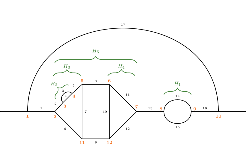
Figure 1: The same diagram as in Eq. (5.16), with additional indications of subdiagrams $H_{i}$ $(i=1\ldots 6)$ which define a example maximal forest.

In this way we can generally construct what is called a maximal forest. In general, the definition of a forest is a set of 1PI subgraphs of $G$ which are non-overlapping, i.e. either disjoint or nested. A maximal forest is thus a maximal set of 1PI subgraphs which are non-overlapping. The above construction illustrates how one can construct all such maximal forests, and it illustrates that each maximal forest contains as many elements as there are loops in $G$.

The example also illustrates that each subgraph $H_{i}$ in a maximal forest contains at least one line that is specific to it, i.e. that is not contained in any smaller subgraphs of the maximal forest. We may define a mapping, called “labelling” in Ref. [4], of the form

$$H_{i} \mapsto\sigma(H_{i})=\text{one of the lines specific to subgraph $H_{i}$.}$$ (5.17)

In the example, we can choose

$$\sigma(H_{1}) =14 \sigma(H_{2}) =3 \sigma(H_{3}) =7$$ (5.18a)

$$\sigma(H_{4}) =11 \sigma(H_{5}) =8 \sigma(H_{6}) =16.$$ (5.18b)

The labelled lines are illustrated in blue colour in the diagram of Fig. 2.

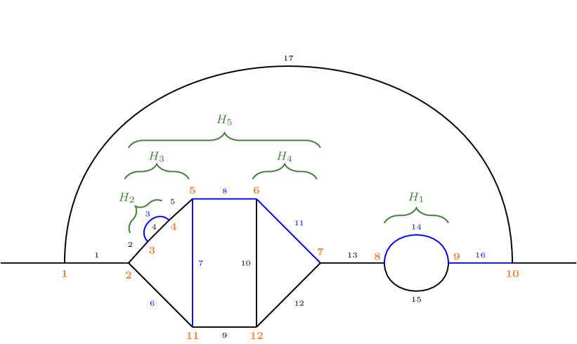
Figure 2: The same diagram as in Fig. 1, with additional indications of the labelled lines $\sigma(H_{i})$ for each subgraph, according to Eq. (5.18).

For any such choice of a maximal forest together with a labelling for specific lines, $(\cal C,\sigma)$, we define an integration sector for the $\alpha_{l}$ variables in the following way: in each subgraph $H_{i}$, the $\alpha$ for the specific labelled line is the largest, i.e.

$$\alpha_{l} \leq\alpha_{\sigma(H_{i})}\ \forall\ l\in H_{i}\,.$$ (5.19)

For the example the integration sector defined by $(\cal C,\sigma)$ is

$$\alpha_{15} \leq\alpha_{14} \alpha_{4} \leq\alpha_{3} \alpha_{2,3,5,6} \leq\alpha_{7}$$ (5.20a)

$$\alpha_{10,12} \leq\alpha_{11} \alpha_{7,11,9} \leq\alpha_{8} \alpha_{1,14,8,13,17} \leq\alpha_{16}\,.$$ (5.20b)

Note that this does not imply a fixed ordering of all the $\alpha_{l}$.

It is elementary to prove a variety of useful properties of maximal forests and labellings. In particular, this way of defining sectors leads to a partitioning of the entire $\alpha$ integration region of any Feynman graph loop integral,

$$\int_{0}^{\infty}d\alpha_{1}\ldots d\alpha_{I} =\sum_{(\cal C,\sigma)}\int_{(\cal C,\sigma)}d\alpha_{1}\ldots d\alpha_{I}\,.$$ (5.21)

Using the notation ${\cal T}_{G}$ for the regularized amplitude of the graph G, we can therefore write

$${\cal T}_{G} =\sum_{(\cal C,\sigma)}{\cal T}_{G,(\cal C,\sigma)}\,,$$ (5.22)

with an obvious meaning and where the sum extends over all maximal forests of $G$ and all possible labellings $(\cal C,\sigma)$. This construction of sectors is the essential content of Lemma 3 in Ref. [4].

5.2.4 Ingredient 2: Forest formula after decomposition into sectors

In the all-order investigation of renormalization, the graphical language of Feynman diagrams with counterterms has to be formalized in terms of subtractions of divergent integrals. In the historical development of the rigorous BPHZ renormalization, this formalization was first performed via Bogoliubov’s recursive definition of the so-called $R$-operation. This recursive definition was later rewritten into Zimmermann’s forest formula [115]. The sector decomposition described above permits a very elegant and powerful alternative version of the forest formula, which simplifies the proof. Such simplified forest formulas were also discussed and applied in the context of BPHZ e.g. in Refs. [66, 114, 123].

To explain these relations we begin with the recursive $R$-operation, defined in Eqs. (5.12,5.13). We recall the main equation, the definition of a subrenormalized amplitude,

$$\overline{\cal R}_{G} =G+\sum_{H_{1}\ldots H_{s}}{G/_{H_{1}\cup\ldots\cup H_{s}}}\cdot C(H_{1})\ldots C(H_{s})\,,$$ (5.23)

where the counterterms are defined as $C(H)=-T\overline{\cal R}_{H}$.

This $R$-operation is recursive because the definition of the subrenormalized amplitude depends on lower-order counterterms which in turn are defined via lower-order subrenormalized amplitudes. One may work out the recursion and obtain a direct, non-recursive formula. To illustrate this, consider the case where the full graph $G$ has one 2-loop subgraph $\gamma_{2}$, which in turn has a 1-loop subgraph $\gamma_{1}$. Then one term in $\overline{\cal R}_{G}$ is given by

$$\overline{\cal R}_{G} =\ldots+{G/_{\gamma_{2}}}\cdot C(\gamma_{2})$$

$$=\ldots+{G/_{\gamma_{2}}}\cdot[-T\overline{\cal R}(\gamma_{2})]$$

$$=\ldots+{G/_{\gamma_{2}}}\cdot[-T({\gamma_{2}}+{\gamma_{2}/_{\gamma_{1}}}\cdot C(\gamma_{1})+\ldots)]$$

$$=\ldots+{G/_{\gamma_{2}}}\cdot[-T{\gamma_{2}}+T({\gamma_{2}/_{\gamma_{1}}}\cdot T{\gamma_{1}})+\ldots]\,.$$ (5.24)

Hence, working out the recursion leads to subtraction operators $T$ acting on unrenormalized (potentially multiloop) graphs like $\gamma_{2}$ and to iterated subtractions. If we introduce a new notation $T_{\gamma}\cdot G\equiv G/_{\gamma}\cdot T\gamma$ for the operation “replace $\gamma$ within $G$ by $T\gamma$”, where products are defined as e.g. $T_{\gamma_{2}}\cdot T_{\gamma_{1}}\cdot G=G/_{\gamma_{2}}\cdot T(T_{\gamma_{1}}\cdot\gamma_{2})$, then we can rewrite the above terms as

$$\ldots+G-T_{\gamma_{2}}\cdot G+T_{\gamma_{2}}\cdot T_{\gamma_{1}}\cdot G\,.$$ (5.25)

We note that both the subgraph $\{\gamma_{2}\}$ as well as the chain of subgraphs $\{\gamma_{1},\gamma_{2}\}$ constitute forests in the sense defined above.

In general, if $\gamma_{1}$ and $\gamma_{2}$ are subgraphs and elements of a forest of $G$, we define

$$\gamma_{2}\supsetneq\gamma_{1} T_{\gamma_{2}}\cdot T_{\gamma_{1}}\cdot G =G/_{\gamma_{2}}\cdot T(T_{\gamma_{1}}\cdot\gamma_{2})$$: (5.26a)

$$\gamma_{1} \gamma_{2} T_{\gamma_{2}}\cdot T_{\gamma_{1}}\cdot G =G/_{\gamma_{1}\cup\gamma_{2}}(T\gamma_{1})(T\gamma_{2})$$, disjoint: (5.26b)

while the product $T_{\gamma_{2}}\cdot T_{\gamma_{1}}$ is undefined for the case when $\gamma_{2}$ is subgraph of $\gamma_{1}$. Working out the recursion formula in general leads to the following forest formula [115]

$${\cal R}(G) =\sum_{\begin{array}[]{c}\scriptstyle{\cal F}=\text{forest}\\ \scriptstyle\text{of $G$}\end{array}}\prod_{\gamma_{i}\in{\cal F}}(-T_{\gamma_{i}})\cdot G\,,$$ (5.29)

where the forests may contain the full graph $G$ and where also the empty set is an allowed forest ${\cal F}=\emptyset$. The formula for $\overline{\cal R}(G)$ is similar but the forests may not contain the full graph $G$. The $T_{\gamma_{i}}$-operators are by definition always ordered as in Eqs. (5.25,5.26) according to nesting. Simply put: operators with bigger subgraphs act on the left, operators with subgraphs contained in the bigger subgraphs on the right. The forest formula can be easily proven by noting that every forest that does not contain $G$ itself has certain disjoint maximal elements $M_{1}\ldots M_{s}$ and can be partitioned into forests of the $M_{1}\ldots M_{s}$. Based on this, the equivalence to the recursive formula can be established by induction over the number of loops.

Now we turn to the announced elegant simplification of the forest formula due to the sector decomposition. We need to know one additional statement about sectors relevant for combinations like

$$T_{\gamma}\cdot G =G/_{\gamma}\cdot T(\gamma)=\sum_{\begin{array}[]{c}(\scriptstyle{\cal C}_{1},\sigma_{1})\\ \scriptstyle\text{for }G/_{\gamma}\end{array}}\sum_{\begin{array}[]{c}\scriptstyle({\cal C}_{2},\sigma_{2})\\ \scriptstyle\text{for }{\gamma}\end{array}}(G/_{\gamma})_{({\cal C}_{1},\sigma_{1})}\cdot T(\gamma_{({\cal C}_{2},\sigma_{2})})\,.$$ (5.34)

The statement is that there is a one-to-one correspondence between such combinations for sectors $({\cal C}_{1},\sigma_{1})$, $({\cal C}_{2},\sigma_{2})$ for the graphs $G/_{\gamma}$ and $\gamma$ and sectors $({\cal C},\sigma)$ for the full graph with the constraint that $\gamma\in{\cal C}$. Then we can split the forest formula into sectors as follows,

$${\cal R}(G) =\sum_{\begin{array}[]{c}\scriptstyle{\cal F}=\text{forest}\\ \scriptstyle\text{of $G$}\end{array}}\sum_{\begin{array}[]{c}\scriptstyle({\cal C},\sigma)\text{ for $G$ which}\\ \scriptstyle\text{contain all $\gamma\in{\cal F}$}\end{array}}\prod_{\gamma_{i}\in{\cal F}}(-T_{\gamma_{i}}|_{\text{subsector }})\cdot G|_{{\text{subsector}}}\,,$$ (5.39)

where it is used that every sector $({\cal C},\sigma)$ with the given constraint generates appropriate subsectors for all subtraction operators $T_{\gamma_{i}}$ and the remaining reduced graph, and that all possible subsectors are generated in this way. Abbreviating slightly we can then rearrange as

$${\cal R}(G) =\sum_{{\cal F}}\quad\sum_{{\cal C}\supseteq{\cal F}}\quad\prod_{\gamma_{i}\in{\cal F}}(-T_{\gamma_{i}})\cdot G$$

$$=\sum_{{\cal C}}\quad\sum_{{\cal F}\subseteq{\cal C}}\quad\prod_{\gamma_{i}\in{\cal F}}(-T_{\gamma_{i}})\cdot G$$

$$=\sum_{{\cal C}}\quad\prod_{\gamma_{i}\in{\cal C}}(1-T_{\gamma_{i}})\cdot G\,.$$ (5.40)

The last step has used that the sum over all possible forests ${\cal F}$ which are contained in ${\cal C}$ effectively generates the power set of ${\cal C}$, i.e. the set of all possible subsets of ${\cal C}$. This simply leads to the last line, which contains only a summation over all maximal forests ${\cal C}$ and the factors $(1-T_{\gamma_{i}})$. In this way the forest formula becomes

$${\cal R}(G) =\sum_{({\cal C},\sigma)}{\cal R}(G)_{({\cal C},\sigma)}\,,$$ (5.41a)

$${\cal R}(G)_{({\cal C},\sigma)} =\prod_{\gamma_{i}\in{\cal C}}(1-T_{\gamma_{i}})\cdot G|_{({\cal C},\sigma)}\,.$$ (5.41b)

The ordering of the $(1-T_{\gamma_{i}})$-operators is as in the original forest formula, according to the nesting of subgraphs.

This represents an important improvement. The operators $(1-T_{\gamma_{i}})$ have the effect of replacing an object by the one without the subdivergences from the subgraph $\gamma_{i}$ (in the appropriate sector). Intuitively, every such operator improves the finiteness. On a more technical level, consider what any specific $T_{\gamma}$ for a multiloop subgraph $\gamma$ acts onto. In the original forest formula, there are terms such as $T_{\gamma}\cdot G$ which lead to $G/_{\gamma}\cdot T(\gamma)$. The $T(\gamma)$ is the divergence of the unrenormalized multiloop graph $\gamma$, which is typically a very complicated expression, non-polynomial in momentum space, or non-local in position space. In contrast, in the forest formula modified for sectors, any such multiloop $T_{\gamma}$ only acts onto expressions where all subdivergences corresponding to subgraphs of $\gamma$ have already been subtracted:

$$T_{\gamma}\prod_{\gamma_{i}\in{\cal C},\gamma_{i}\subsetneq\gamma}(1-T_{\gamma_{i}})\cdot G_{({\cal C},\sigma)} =T\left(\prod_{\gamma_{i}\in{\cal C},\gamma_{i}\subsetneq\gamma}(1-T_{\gamma_{i}})\cdot\gamma\right)\cdot G_{({\cal C},\sigma)}$$ (5.42)

Hence here the left-most $T$ actually acts on the fully subrenormalized expression $\overline{\cal R}(\gamma)$ in the appropriate subsector, which can be hoped to have simpler, polynomial/local divergences. These properties of the forest formula help in setting up an inductive proof of renormalization.

5.2.5 Ingredient 3: Sector Variables and Formula for the Integral

Introducing sectors into the $\alpha$ integrations required for Feynman graph integrals has further important advantages. Besides yielding the simpler forest formula, the sectors allow rewriting the actual integrals such that the power counting and the structure of divergences are isolated in a quite transparent way. Here we illustrate this in a very simple case; then we provide the general result and give comments.

Let us focus on the integral (3.36), $(4\pi)^{-D/2}i^{1-D/2}\int_{0}^{\infty}d\alpha_{1}d\alpha_{2}{\cal U}^{-D/2}e^{iW}$ and consider the sector $\alpha_{1}\leq\alpha_{2}$. In this sector we introduce sector-specific variables: the largest $\alpha$ in the sector is replaced by a new variable $t^{2}$, the other $\alpha$ is rewritten as $t^{2}\beta$ in terms of a scaling variable $\beta$ which runs from 0 to 1. In total we carry out the following substitution of variables and the integration measure in the sector

$$\alpha_{2} =t^{2}\,,$$ (5.43a)

$$\alpha_{1} =t^{2}\beta\,,$$ (5.43b)

$$\int_{0\leq\alpha_{1}\leq\alpha_{2}}d\alpha_{1}d\alpha_{2} =2\int_{0}^{\infty}dtt^{(2I-1)}\int_{0}^{1}d\beta\,,$$ (5.43c)

where $I=2$ is the number of internal lines. The integral (3.36) depends on two functions, the Symanzik polynomial ${\cal U}$ and the exponent $W$ given in Eq. (3.39). After the variable substitution the Symanzik polynomial takes the value

$${\cal U} =M=t^{2}(1+\beta)\,,$$ (5.44)

and we observe that we can factor out the variable $t^{2}$. This is no accident. As already mentioned in Sec. 3.2.4, the behaviour of ${\cal U}$ if some $\alpha$’s vanish reflects the ultraviolet behaviour of the original Feynman integral. If all $\alpha$’s simultaneously vanish $\propto t^{2}$, ${\cal U}$ generally behaves as $t^{2L}$, where $L$ is the number of loops in the graph. We can exhibit this behaviour by defining a new function $\tilde{d}$

$${\cal U} =t^{2}\tilde{d}\,, \tilde{d} =1+\beta\geq 1\,.$$ (5.45)

The indicated inequality provides a very important lower bound on the function $\tilde{d}$.

A second observation is that we can essentially eliminate the $t$-variable from the exponent $W$ by rescaling the physical variables $p$, $u_{1,2}$ and $m$ as

$$\tilde{p} =t\,p\,,$$ (5.46a)

$$\tilde{m} =t\,m\,,$$ (5.46b)

$$\tilde{u}_{1,2} =t^{-1}\,u_{1,2}\,.$$ (5.46c)

The rescaled variables are dimensionless. In terms of these variables we can write the exponent as

$$W =\frac{\tilde{p}^{2}\beta-\beta\tilde{u}_{2}\cdot\tilde{p}+\tilde{u}_{1}\cdot\tilde{p}-\frac{1}{4}(\tilde{u}_{1}+\tilde{u}_{2})^{2}}{(1+\beta)}+(it^{2}\varepsilon-\tilde{m}^{2})(1+\beta)\,,$$ (5.47)

where indeed $t$ does not appear explicitly, except in the product $t^{2}\varepsilon$.

Using all these ingredients we can rewrite the $\alpha$ integral (3.36) in the considered sector as

$$(-i)^{2}(4\pi)^{-D/2}i^{1-D/2}2\int_{0}^{\infty}dtt^{-D+2I-1}\int_{0}^{1}d\beta\tilde{d}^{-D/2}e^{iW}\,,$$ (5.48)

where we record the following observations:

• The power-like behaviour of $\int dtt^{-D+2I-1}$ corresponds to the superficial ultraviolet power counting of the original loop integral (3.36) which behaves like $\int d^{D}kk^{-2I}$.

• The remaining integrand $\tilde{d}^{-D/2}e^{iW}$ has essentially no explicit dependence on $t$ at all; it only depends on $t$ via the rescaled variables (5.46) and via $t^{2}\varepsilon$.

• If $\varepsilon>0$ in the $+i\varepsilon$ prescription, $e^{iW}$ decreases exponentially for large $t$, and the full dependence of the integrand on the rescaled variables (5.46) and on $\beta$ is of $C^{\infty}$-type. The result of the $\beta$ integration is still $C^{\infty}$ in the rescaled variables.

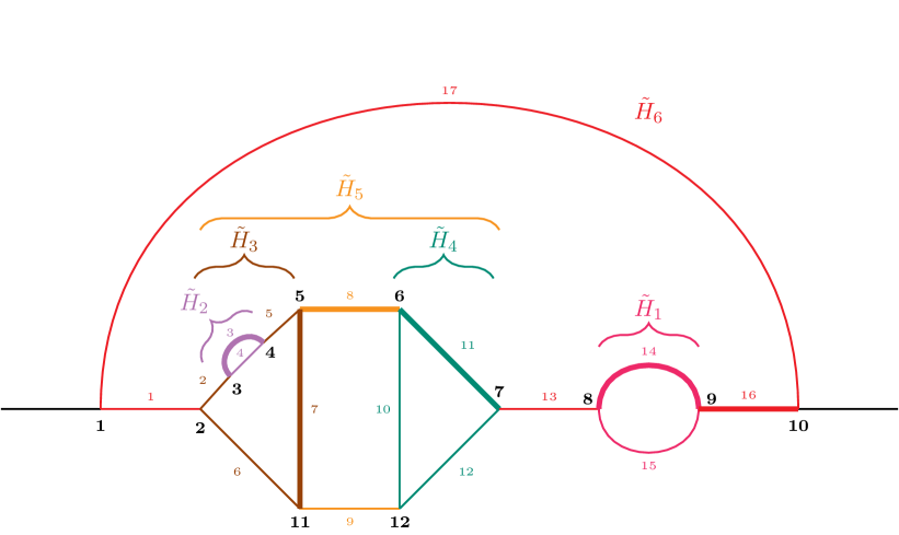
Figure 3: Illustration of sectors and sector variables $t$ and $\beta$ in Eqs. (5.49,5.50). The example is the 6-loop diagram and its subdiagrams already used in Eq. (5.16) and Figs. 1, 2. Here we choose six different colours for the reduced subdiagrams $\bar{H}_{i}$ $(i=1\ldots 6)$ into which the diagram can be partitioned.

We need a second example to shape our understanding of the general case. Let us consider again the 6-loop diagram of Sec. 5.2.3 and fix the same sector $({\cal C},\sigma)$ discussed there, see Eq. (5.20). Which variable substitutions analogous to Eqs. (5.43,5.46) should we now choose? The sector is defined by a maximal forest with six subgraphs, each subgraph contains one specific labelled line, and for each subgraph there is an inequality stating that the labelled $\alpha$ is the largest. The idea, generalizing the 1-loop case, is to introduce one $t_{i}$-variable for each subgraph $H_{i}$ and to define the labelled $\alpha$’s in terms of these $t_{i}$-variables. The $t_{6}\equiv t_{G}$-variable corresponding to the full graph runs from $0$ to $\infty$, and all the other $t_{i}$ run from $0$ to $1$. Then all inequalities for the labelled $\alpha$’s are implemented by the following scheme:

subgraph: label led $$\alpha$$ substitution: re write

$$H_{1} \alpha_{14} =t_{1}^{2}t_{6}^{2} t_{1}^{2}\xi_{1}^{2}$$ (5.49a)

$$H_{2} \alpha_{3} =t_{2}^{2}t_{3}^{2}t_{5}^{2}t_{6}^{2} t_{2}^{2}\xi_{2}^{2}$$ (5.49b)

$$H_{3} \alpha_{7} =\quad t_{3}^{2}t_{5}^{2}t_{6}^{2} t_{3}^{2}\xi_{3}^{2}$$ (5.49c)

$$H_{4} \alpha_{11} =\quad t_{4}^{2}t_{5}^{2}t_{6}^{2} t_{4}^{2}\xi_{4}^{2}$$ (5.49d)

$$H_{5} \alpha_{8} =\quad\quad t_{5}^{2}t_{6}^{2} t_{5}^{2}\xi_{5}^{2}$$ (5.49e)

$$H_{6} \alpha_{16} =\quad\quad\quad t_{6}^{2} t_{6}^{2}\xi_{6}^{2}$$ (5.49f)

where also abbreviation variables $\xi_{i}$ were introduced; they are products of all the “other $t_{i}$”, as appropriate. In the next step we introduce $\beta_{k}$-variables for all the remaining, non-labelled, $\alpha$’s, where the $\beta_{k}$ all run from $0$ to $1$. We remark that $t_{6}\equiv t_{G}$ is dimensionful, while all other $t_{i}$ and $\beta$ variables are dimensionless. In addition we introduce two further useful notations, illustrated in the graph in Fig. 3. First, for each subgraph in ${\cal C}$ we define a reduced subgraph $\bar{H}_{i}=H_{i}/_{{\cal M}(H_{i})}$, where ${\cal M}(H_{i})$ is the set of maximal elements in ${\cal C}$ which are properly contained in $H_{i}$. The lines in $\bar{H}_{i}$ are the lines specific to $H_{i}$, i.e. the lines contained in $H_{i}$ but in no smaller subgraph in ${\cal C}$. Clearly, the full graph is partitioned into $\bar{H}_{i}$, i.e. every line is in one unique $\bar{H}_{i}$. Second, we denote by $\underline{q}_{H_{i}}$ a set of independent external momenta of $\bar{H}_{i}$, where we in principle allow nonzero incoming momenta into all vertices of the graph (the graph is drawn as if it has only two external momenta, but the renormalization procedure becomes more systematic if every graph is generalized to allow arbitrary incoming momenta into all vertices). This leads to the following scheme:

red.  subgraph: $$\alpha$$’s indep. ext. momenta

$$\bar{H}_{1} =H_{1} \{\alpha_{15},\alpha_{14}\} =\{\beta_{15},1\}\times t_{1}^{2}\xi_{1}^{2} p_{8}$$ (5.50a)

$$\bar{H}_{2} =H_{2} \{\alpha_{4},\alpha_{3}\} =\{\beta_{4},1\}\times t_{2}^{2}\xi_{2}^{2} p_{3}$$ (5.50b)

$$\bar{H}_{3} =H_{3}/_{H_{2}} \{\alpha_{2,5,6},\alpha_{7}\} =\{\beta_{2,5,6},1\}\times t_{3}^{2}\xi_{3}^{2} p_{2},p_{5},p_{11}$$ (5.50c)

$$\bar{H}_{4} =H_{4} \{\alpha_{10,12},\alpha_{11}\} =\{\beta_{10,12},1\}\times t_{4}^{2}\xi_{4}^{2} p_{6},p_{7}$$ (5.50d)

$$\bar{H}_{5} =H_{5}/_{H_{3}\cup H_{4}} \{\alpha_{9},\alpha_{8}\} =\{\beta_{9},1\}\times t_{5}^{2}\xi_{5}^{2} p_{6}+p_{7}+p_{12}$$ (5.50e)

$$\bar{H}_{6} =H_{6}/_{H_{5}\cup H_{1}} \{\alpha_{1,13,17},\alpha_{16}\} =\{\beta_{1,13,17},1\}\times t_{6}^{2}\xi_{6}^{2} p_{1},p_{8}+p_{9},p_{10}$$ (5.50f)

The reduced subgraphs $\tilde{H}_{i}$ are formed solely by the lines proper to them, and lines shared amongst the $H_{i}$ are shrunk to a point. The subgraphs $H_{1},H_{2},H_{4}$ are identical to the reduced ones and hence take the obvious form as depicted in Fig. 3. In the case of $H_{3},H_{5},H_{6}$, the reduced subgraphs are obtained by shrinking different subgraphs to a point. Let us illustrate this by specifying the form of these reduced subgraphs as follows:

(5.51)

The crossed dots of order $(n)$ denote the counterterm insertion due to shrinking the respective $n$-loop subgraph to a point. Since we assume that to each vertex $V_{i}$ there is associated an entering momentum $p_{i}$, shrinking a subgraph comprised of vertices $V_{i_{1}},\dots,V_{i_{k}}$, leads to a combination of incoming momenta $p_{i_{1}}+\dots+p_{i_{k}}$ for that counterterm vertex, as indicated in the graphs. In choosing independent momenta, we can make use of momentum conservation. For a reduced subgraph with $n$ vertices, it is sufficient to specify $n-1$ incident momenta to the vertices. They uniquely characterize the momenta of a given reduced subgraph. What is more, all momenta of the graph can be reconstructed by linear combinations of these independent external momenta. A specific choice is given in Eq. (5.50). Clearly, in this way all inequalities of the sector (5.20) are implemented and the combination of all the selected independent incoming momenta of the $\bar{H}_{i}$ span all independent incoming momenta of the full graph and can be used as independent variables in the result. The variable substitution leads to the following replacement of the integration measure, analogous to Eq. (5.43),

$$\int_{({\cal C},\sigma)}d\alpha_{1}\ldots d\alpha_{17} =2^{L}\int_{\begin{subarray}{c}t_{6}=0\ldots\infty\\ t_{1\ldots 5}=0\ldots 1\end{subarray}}\prod_{i=1}^{6}dt_{i}t_{i}^{(2I_{H_{i}}-1)}\int_{0}^{1}\prod_{k}d\beta_{k}\,,$$ (5.52)

where $I_{H_{i}}$ is the number of internal lines in $H_{i}$.

This example provides us with sufficient information to construct the general result for the integral representation of a general 1PI graph $G$ in a specific sector $({\cal C},\sigma)$. As in the example, the sector defines a chain of subgraphs $H_{i}$ (as many as there are loops; one of them is equal to the full graph $G$). The sector also defines a particular replacement of all $\alpha$’s in terms of $t_{i}$ and $\beta_{k}$; for each subgraph $H_{i}$ it is also useful to define the variable $\xi_{i}$ for the product of all the “other $t_{i}$”. All lines of $G$ are partitioned into lines of the reduced graphs $\bar{H}_{i}$, and for each $\bar{H}_{i}$ one can choose a set of independent incoming momenta $\underline{q}_{H_{i}}$, which in total span all incoming momenta of the full graph. Since each line carries one mass variable and one $u$-variable, we can also partition these variables into sets of masses $m_{H_{i}}$ and sets of $u$’s, $u_{H_{i}}$, corresponding to the respective $\bar{H}_{i}$.

With these variables we can rescale physical quantities, generalizing Eq. (5.46), as

$$\tilde{\underline{q}}_{H_{i}} =t_{i}\xi_{i}\underline{q}_{H_{i}}\,,$$ (5.53a)

$$\tilde{m}_{H_{i}} =t_{i}\xi_{i}m_{H_{i}}\,,$$ (5.53b)

$$\tilde{u}_{H_{i}} =(t_{i}\xi_{i})^{-1}u_{H_{i}}\,.$$ (5.53c)

We allow the integral to contain a numerator expressed as a derivative with respect to $u$-variables as in Eqs. (3.37,3.38a), but we assume that the derivative operator $Z$ in the numerator is a product of $Z_{H_{i}}$, where each $Z_{H_{i}}$ only depends on variables specific to $\bar{H}_{i}$. This is always the case in actual Feynman diagrams. For simplicity we follow Ref. [4] and assume that all $Z_{H_{i}}$ are homogeneous polynomials in the variables $\partial/\partial u_{H_{i}}$ and $m_{H_{i}}$ of some degree $r_{\bar{H}_{i}}$. Then we can write

$$\tilde{Z}_{H_{i}} =(t_{i}\xi_{i})^{r_{\bar{H}_{i}}}{Z}_{H_{i}}$$ (5.54)

where $\tilde{Z}_{H_{i}}$ is the same homogeneous polynomial expressed with $\partial/\partial\tilde{u}_{H_{i}}$ and $\tilde{m}_{H_{i}}$. Writing $D=4-2\epsilon$ we can finally define a power-counting degree of each reduced subgraph $\bar{H}_{i}$ and the complete (sub)graphs $H_{i}$ as

$$\omega_{\bar{H}_{i}} =4L_{\bar{H}_{i}}-2I_{\bar{H}_{i}}+r_{\bar{H}_{i}}\,,$$ (5.55a)

$$\omega_{H_{i}} =\sum_{\begin{subarray}{c}H^{\prime}\subseteq H_{i}\\ H^{\prime}\in{\cal C}\end{subarray}}\omega_{\bar{H}^{\prime}}\,.$$ (5.55b)

This clearly corresponds to the superficial power-counting degree of the original momentum integral.

With these building blocks we can formulate the general result for the integral specified in Eqs. (3.37,3.38a). Decomposing the integral in sectors as in Eq. (5.22),

$${\cal T}_{G} =\sum_{({\cal C},\sigma)}{\cal T}_{G,({\cal C},\sigma)}\,,$$ (5.56)

and setting again $D=4-2\epsilon$, the result for each sector can be written as

$${\cal T}_{G,({\cal C},\sigma)} =c_{D}^{L}2^{L}\int_{\begin{subarray}{c}t_{L}=0\ldots\infty\\ t_{1\ldots L-1}=0\ldots 1\end{subarray}}\prod_{i=1}^{L}\frac{dt_{i}}{t_{i}}(t_{i}\xi_{i})^{-\omega_{\bar{H}_{i}}+2\epsilon}\tilde{Z}_{H_{i}}$$

$$\qquad\times\int_{0}^{1}\prod_{k}d\beta_{k}\tilde{d}_{G}^{-D/2}e^{iW_{G}}\Bigg{|}_{u=0}\,.$$ (5.57)

The properties of the appearing objects are:

• All variables $t_{i}$, $\xi_{i}$, $\beta_{k}$ and the rescaled physical variables $\tilde{\underline{q}}_{H_{i}}$, $\tilde{m}_{H_{i}}$, $\tilde{u}_{H_{i}}$, and the power-counting degrees $\omega_{\bar{H}_{i}}$ are defined above.

• The explicit powers of $t_{i}$ correspond to the original superficial power-counting degrees of the momentum integrals over the subdiagrams $H_{i}$. For each $t_{i}$ integral, a factor $(t_{i}\xi_{i})^{2\epsilon}$ was split off which may be viewed as the essence of the $D$-dimensional integration measure.

• The remaining integrand $\tilde{d}_{G}^{-D/2}e^{iW_{G}}$ has no explicit dependence on $t_{L}$ at all. It depends on $t_{L}$ only via the rescaled physical variables. The other $t_{i}$ with $i=1\ldots L-1$ typically appear explicitly, however.

• The function $\tilde{d}_{G}$ is a rescaled Symanzik polynomial which satisfies $\tilde{d}_{G}\geq 1$ in the integration region.

• For $\varepsilon>0$ in the $+i\varepsilon$ prescription, the function $e^{iW_{G}}$ is exponentially decreasing for large $t_{L}$.

• The product $\tilde{d}_{G}^{-D/2}e^{iW_{G}}$, therefore, is analytic in $\epsilon$ and $C^{\infty}$ in $t_{i}$, $\beta_{k}$ and the rescaled physical variables $\tilde{\underline{q}}_{H_{i}}$, $\tilde{m}_{H_{i}}$, $\tilde{u}_{H_{i}}$.

This statement is the starting point for the inductive proof of renormalization in DReg given in Ref. [4], and it is a direct consequence of Lemma 4 of that reference.

5.2.6 Ingredient 4: Integrand Relation between Graphs and Subgraphs

An important step in the proof is the application of subtraction operators $T_{H}$ to a graph $G$. In order to analyze this operation, relationships between the original graph $G$, the reduced graph $G/_{H}$ and the subgraph $H$ are needed. These relationships are again essentially independent of $D$-dimensional treatments. They rely on detailed analysis of the graphs themselves, and the relationships between graphs and the $\alpha$-parametrizations.

The required theory involves incidence matrices and graph theoretical representations of the Symanzik polynomial ${\cal U}$, or $\tilde{d}_{G}$, and the exponent $W_{G}$. Although the theory is very elegant and not too difficult we do not develop it here. Hence we only list several important statements without proof. For the proofs we refer to Ref. [4] and references therein. Further discussions were given e.g. in Refs. [69, 51, 124]

Consider the Symanzik polynomial ${\cal U}_{G}$ for a graph $G$, and let $H$ be a subgraph of $G$. ${\cal U}$ is a homogeneous polynomial in all $\alpha$’s of degree $L$. Consider the case where all $\alpha$’s corresponding to the subgraph $H$ are rescaled by a factor $\rho$, while all other $\alpha$’s remain fixed. Then, for small $\rho$ we have

$${\cal U}_{G}(\text{$\alpha$'s in $H$ rescaled by $\rho$}) =\underbrace{{\cal U}_{G/_{H}}}_{\text{$\rho$-independent}}\quad\underbrace{{\cal U}_{H}}_{\propto\rho^{L_{H}}}+{\cal O}(\rho^{L_{H}+1})\,,$$ (5.58)

i.e. at the lowest non-vanishing order the Symanzik polynomial factorizes into the two individual Symanzik polynomials for the reduced graph and the subgraph. If $G$ and $H$ are part of an integration sector as defined above, then variables $t_{G}$, $t_{H}$ (and possibly further $t_{i}$) and $\beta_{k}$ exist and rescaled Symanzik polynomials $\tilde{d}$ can be defined for each of these graphs. In this case, $\tilde{d}_{G}$ for the full graph cannot depend on $t_{G}$ but it can depend on $t_{H}$, while $\tilde{d}_{G/_{H}}$ and $\tilde{d}_{H}$ can neither depend on $t_{G}$ nor on $t_{H}$. Their relationship is the factorization

$$\tilde{d}_{G}|_{t_{H}=0} =\tilde{d}_{G/_{H}}\tilde{d}_{H}\,.$$ (5.59)

A similar relationship can be established for the exponent $W_{G}$ appearing in the general result of the integral (5.57). Defining $W_{H}$ and $W_{G/_{H}}$ using the same variable transformations for the sector $({\cal C},\sigma)$, suitably adapted to the subgraph and reduced graph, the relationship is

$$W_{G}|_{t_{H}=0} =W_{G/_{H}}+W_{H}|_{t_{H}=0}\,,$$ (5.60)

if all these quantities are expressed in terms of rescaled variables $\tilde{\underline{q}}$, $\tilde{u}$, $\tilde{m}$. This property can be established in an elementary way once the exponents are constructed via incidence matrices.

For the same conditions, a further, more intricate property can also be established and is important. It is the following property involving derivatives,

$$\frac{d}{dt_{H}}\tilde{d}_{G}^{-D/2}e^{iW_{G}}\Bigg{|}_{t_{H}=0} =\xi_{H}U_{H}\left[\frac{d}{dt_{H}}\tilde{d}_{H}^{-D/2}e^{iW_{H}}\right]_{t_{H}=0}\cdot\tilde{d}_{G/_{H}}^{-D/2}e^{iW_{G/_{H}}}\,.$$ (5.61)

Here $U_{H}[X]$ denotes an insertion operator which effectively inserts its argument $X$ as a vertex into a bigger graph. To achieve this insertion, the external momenta of the argument $X$ must become internal momenta of the bigger graph, in this case of $G/_{H}$. Technically, $U_{H}$ acts by shifting in its argument the momentum variables $\tilde{\underline{q}}_{H}$ by terms involving derivatives with respect to $u$-variables for the bigger graph $G/_{H}$.

This is a statement of pivotal importance for the full proof of the theorem stated in Sec. 5.2.1 since it allows relating divergences of a full graph to divergences of counterterm graphs and thus allows making manifest the cancellation of subdivergences. It is essentially the content of Lemma 5 of Ref. [4].

5.2.7 Ingredient 5: Simple Integrals and Non-Analytic Functions of $D-4$

Now we discuss several simple integrals and special functions that arise in DReg due to the $D$-dimensionality of spacetime. They encapsulate how the regularization acts, how divergences arise as $1/(D-4)$ poles and how divergences cancel by adding suitable counterterms. We set again $D=4-2\epsilon$.

First we discuss a simple type of integral, defined as

$$f(z) =\int_{0}^{\infty}dtt^{z-1}g(t)\,,$$ (5.62)

where $z$ is a complex variable and $g(t)$ is a $C^{\infty}$ function which either decreases exponentially for $t\to\infty$ or which involves the step function $\theta(1-t)$ cutting off the integral at $t=1$. This simple integral appears in the general result (5.57) but also in the 1-loop example (5.48). In all these cases the $t$-integration involves one factor which is of the form $t^{n-1+2\epsilon}$, where $n$ is an integer. This corresponds to the above form for $z=n+2\epsilon$. This factor is non-analytic in $t$ around $t=0$. The remaining $t$-dependences in Eqs.  (5.57,5.48) are complicated but are $C^{\infty}$ functions in $t$ which indeed fulfil the requirements on $g(t)$ listed above. In case of the $t_{L}$ integration, the remaining integrand exponentially decreases, in case of all other $t_{i}$ integrations, the integration stops at $t_{i}=1$.

The above function $f(z)$ is a generalization of the $\Gamma$-function, where $g(t)=e^{-t}$. The $\Gamma$-function is known to have simple poles at $z=0$, $z=-1$, $z=-2$, …. It is easy to see that the same is true for the more general $f(z)$. Clearly, when for $\text{Re}(z)>0$ the integral defining $f(z)$ converges and defines an analytic function. To study negative $\text{Re}(t)$ we can add to and subtract from $g(t)$ a Taylor polynomial $\sum g^{(k)}(0)t^{k}/k!$, where $g^{(k)}$ denotes the $k$-th derivative. Integrating this polynomial from $0$ to $1$ we obtain

$$f(z) =\int_{0}^{\infty}dtt^{z-1}\left[g(t)-\theta(1-t)\sum_{k=0}^{n}\frac{g^{(k)}(0)}{k!}t^{k}\right]+\sum_{k=0}^{n}\frac{g^{(k)}(0)}{k!}\frac{1}{z+k}\,.$$ (5.63)

For any non-negative integer $n$ and for $\text{Re}(z)>0$ the value and convergence properties of the integral are not changed. However, the square bracket behaves like $t^{n+1}$ for small $t$, hence the integral now converges even for negative $z$, as long as $\text{Re}(z)>-n-1$. Hence this formula represents an analytic continuation of $f(z)$ onto the entire complex $z$ plane. It makes also manifest that this analytically continued $f(z)$ has single poles at $z=-0$, $z=-1$, $z=-2$, ….

We can rewrite the result in the form of an integration rule for the typical $t$-integrals appearing in DReg by replacing $z=-n+2\epsilon$ with integer non-negative $n$ and $\epsilon\approx 0$. We then have the rule

$$\int_{0}^{\infty}dtt^{-n-1+2\epsilon}g(t) =\frac{1}{n!}\left(\frac{d}{dt}\right)^{n}g(t)\Bigg{|}_{t=0}\frac{1}{2\epsilon}+\text{regular expression}\,,$$ (5.64)

where the form of the regular expression can be read off from Eq. (5.63). The $t$-integrals in the general formula (5.57) are to be analytically continued in this way. Hence this rule immediately shows that any $t$-integration can only lead to single $1/\epsilon$-poles and not to more complicated divergences as $\epsilon\to 0$.

Next, we consider two special simple classes of non-analytic functions of $t$. They are defined as the two kinds of sets (for integer $K,L$)

$$K <L: J_{K}^{L} =\left\{f(t,\epsilon)=\frac{c_{1}t^{2\epsilon}+\ldots+c_{L}t^{2L\epsilon}}{\epsilon^{K}}=\text{finite for }\epsilon\to 0\right\}\,,$$ (5.65a)

$$K \leq L: \tilde{J}_{K}^{L} =\left\{f(t,\epsilon)=\frac{c_{0}+c_{1}t^{2\epsilon}+\ldots+c_{L}t^{2L\epsilon}}{\epsilon^{K}}=\text{finite for }\epsilon\to 0\right\}\,.$$ (5.65b)

In the definitions of the sets, the lower index $K$ refers to the $\epsilon$-power in the denominator, and the upper index $L$ can be thought of as the loop number at which the functions become of interest. The coefficients $c_{i}$ are arbitrary except for the constraint that the defined functions are finite for $\epsilon\to 0$.

Let us illustrate how such functions can appear by considering a 2-loop diagram $G$ with a 1-loop subdiagram $H$. We imagine a calculation not only of the diagrams themselves but of the entire renormalization procedure, taking into account suitable counterterm diagrams cancelling subdivergences. In the imagined calculations we use the general formula (5.57). If the 1-loop diagram $H$ is computed in isolation, it involves one $t_{1}$-integral whose essential non-analytic part is simply

$$t_{1}^{2\epsilon}\in J_{0}^{1}\,,$$ (5.66)

which is an element of the set $J_{0}^{1}$ and which may be attributed to the $D$-dimensional measure. The result of the $t_{1}$-integration via the rule (5.64) then leads particularly to a $1/(2\epsilon)$ pole, and a counterterm for diagram $H$ can be defined that cancels this divergence. In the 2-loop calculation of $G$ the 1-loop diagram $H$ appears as a subdiagram with corresponding $t_{1}$ integration. Here the $t_{1}$ variable is accompanied by $\xi_{1}$, which is here simply $\xi_{1}=t_{2}$. After the $t_{1}$ integration, the non-analytic factor $\xi_{1}^{2\epsilon}$ remains and combines with the $1/(2\epsilon)$ pole. In the corresponding counterterm diagram, where the subdiagram $H$ is replaced by the counterterm cancelling its $1/(2\epsilon)$ pole there is no $t_{1}$ integration and no appearance of the variable $\xi_{1}$. Therefore, after the $t_{1}$ integration and after combining with the counterterm diagram cancelling the subdivergence, a combined function

$$\frac{t_{2}^{2\epsilon}-1}{2\epsilon}\in\tilde{J}_{1}^{1}$$ (5.67)

appears. The finiteness of functions in the set $\tilde{J}_{1}^{1}$ reflects the successful cancellation of the subdivergence. Proceeding with the computation of the 2-loop diagram $G$, this function is combined with the measure factor, such that the interesting non-analytic part of the $t_{2}$-integrand is

$$t_{2}^{2\epsilon}\frac{t_{2}^{2\epsilon}-1}{2\epsilon}\in J_{1}^{2}\,.$$ (5.68)

This example illustrates the general idea: Functions in $J_{K}^{L}$ are the functions that actually appear as the non-analytic factors in the $t_{L}$ integrations at the $L$-loop level during the renormalization procedure. After carrying out a $t_{L}$ integral and after combining with the suitable counterterm contribution, a function in the set $\tilde{J}_{K+1}^{L}$ appears. At the next loop level the integrand needs to be prepared by suitable rearrangements and combined with the measure factor $t_{L+1}^{2\epsilon}$ to produce a function of the set $J_{K+1}^{L+1}$, and so on.

For this reason it is helpful to study the properties of functions in these sets on their own, before tackling the actual loop integrations. Some particularly useful properties are:

$(i)$

any function $f\in J_{K}^{L}$ has the limit $f(t,0)=\text{const}\times(\ln t)^{K}$.

$(ii)$

for a function $f\in J_{K}^{L}$, the integral $\int_{1}^{t}\frac{dt^{\prime}}{t^{\prime}}f(t^{\prime},\epsilon)$ produces an element of the next set $\tilde{J}_{K+1}^{L}$.

$(iii)$

the converse is also true, i.e. every element of $\tilde{J}_{K+1}^{L}$ can be written in terms of such an integral.

$(iv)$

a function $f\in J_{K}^{L}$ where the first argument is a product can be factorized as $f(\xi t,\epsilon)=\sum_{j}f_{1j}(\xi,\epsilon)f_{2j}(t,\epsilon)$ where all functions on the right-hand side are elements of $f_{nj}\in J_{K_{nj}}^{L}$ where $K_{1j}+K_{2j}=K$. This property is obviously important to prepare higher-loop integrands such that $t$ integrals act on isolated functions depending only on $t$, not on $\xi$.

$(v)$

there is a simple product rule $f_{K_{1}}^{L_{1}}f_{K_{2}}^{L_{2}}\in J_{K_{1}+K_{2}}^{L_{1}+L_{2}}$ for functions $f_{K_{i}}^{L_{i}}\in J_{K_{i}}^{L_{i}}$. This property is also important on the multiloop level in case a multiloop diagram contains two disjoint divergent subdiagrams.

The properties can all be proved using elementary integration tricks and l’Hopital’s rule for limits. Such properties of these functions are the content of Lemma 2 of Ref. [4].

5.2.8 Sketch of Proof by Induction

All explained ingredients are important in the full proof of the central Theorem 1 in Ref. [4] and stated in Sec. 5.2.1. Here we give a sketch of this proof. The proof applies the $\alpha$ parametrization of integrals decomposed into sectors as in Eq. (5.22). The renormalization procedure is then expressed in terms of the forest formula (5.41). This formula provides the basis for an inductive proof, where a graph $G$ and a sector are fixed and then all factors $(1-T_{H_{i}})$ in the forest formula are successively applied in the correct ordering. The base case of the induction is provided by the general formula (5.57). The induction step needs to carry out the actual integration over one $t$ variable and some $\beta$ variables corresponding to the next $(1-T_{H_{i}})$ factor. The step uses the properties of the special functions of $\epsilon$ defined in Sec. 5.2.7, and the relationships between the graph, subgraph and reduced graph described in Sec. 5.2.6.

Obtaining the precise form of the induction hypothesis is highly nontrivial, but it can be motivated using all the developed insight. It can be formulated as follows. Consider a 1PI graph $G$ and a sector $({\cal C},\sigma)$. All following quantities are specific to this sector but for brevity we will omit all indices denoting this dependence. The graph has $L_{G}$ loops and the sector contains $L_{G}$ subgraphs $H_{1},\ldots,H_{L_{G}}$. Without loss of generality we assume the labelling such that the subgraphs are already ordered according to their allowed appearance in the forest formula (5.41), such that if $H_{j}\supseteq H_{i}$ then also $j\geq i$ (the ordering is not unique). Then after evaluating $L\leq L_{G}$ factors in the forest formula we obtain the expression (suppressing the dependence on the sector $({\cal C},\sigma)$)

$${\cal R}_{X}(G)\equiv(1-T_{H_{L}})\cdot\ldots\cdot(1-T_{H_{2}})\cdot(1-T_{H_{1}})\cdot G\,.$$ (5.69)

This represents a partially renormalized graph where $L$ loops and $L$ subgraphs have already been treated in previous induction steps. Sec. 5.2.4 gave arguments that this expression should have simple divergence properties when acted upon by further $T_{H_{i}}$ operators. Despite this, the partially renormalized expression on its own clearly can have very complicated analytical structure and can still have non-polynomial divergences which the proof needs to deal with. The label $X$ denotes the set of all subgraphs which have already been treated, and we also define $X_{0}$ as the subset of $X$ which contains only maximal subgraphs, i.e.

$$X =\{H_{1},\ldots,H_{L}\}\,, X_{0} =\{M_{1},\ldots,M_{S},H_{L}\}\,,$$ (5.70)

where it is used that $H_{L}$ itself is necessarily a maximal subgraph in $X$ and where names have been given to all other elements of $X_{0}$.

The induction hypothesis states that after evaluating all $t_{i}$ and $\beta_{k}$ integrals corresponding to lines in the already treated graphs in $X$, we obtain

$${\cal R}_{X}(G)={}$$ sum of terms like

$$\int_{\geq L+1}\prod_{M\in X_{0}}\xi_{M}^{-\omega_{M}}\tilde{f}_{M}(\xi_{M},\epsilon)g_{G,X}\Bigg{|}_{\tilde{u}=0}\,,$$ (5.71)

where the integration factors for the remaining integrals are abbreviated as

$$\int_{\geq L+1}={} c_{D}^{L_{G}-L}\int\prod_{i=L+1}^{L_{G}}\frac{dt_{i}}{t_{i}}(t_{i}\xi_{i})^{-\omega_{\bar{H}_{i}}+2\epsilon}\int\prod_{k\in G/_{X_{0}}}d\beta_{k}\tilde{Z}_{H_{i}}\,.$$ (5.72)

Here the integration boundaries of the $t_{i}$ and $\beta_{k}$ integrals are as in Eq. (5.57), and the notation $k\in G/_{X_{0}}$ corresponds to all indices $k$ corresponding to any line outside the already treated graphs in the set $X$. In the product over the maximal subgraphs $M$ (which includes the case $M=H_{L}$), each $M$ is equal to one particular $H_{j(M)}$ and for simplicity we identify the indices $\xi_{M}\equiv\xi_{{j(M)}}$.

We provide the following comments on the induction hypothesis:

• The “sum of terms like” refers to the expression in the integrand which really is of the form $\sum_{a}\prod_{M}\tilde{f}_{M,a}g_{G,X,a}$. Since the proof can be carried out for each such term we drop the index $a$ and this summation.

• The integration variables $t_{i}$ and $\beta_{k}$ and the $\tilde{u}_{k}$ variable for the already treated graphs do not exist anymore since they have been integrated over/set to zero. Hence the only appearing $t_{i}$, $\beta_{k}$ and $\tilde{u}_{k}$ are the ones for $i=L+1,\ldots,L_{G}$ and for $k\in G/_{X_{0}}$.

• The sets of physical variables $\tilde{\underline{q}}_{H_{i}}$, $\tilde{m}_{H_{i}}$ and the remaining $\tilde{u}_{H_{i}}$ (for $H_{i}\notin X$) are rescaled only by the remaining $t_{i}$’s. I.e. Eq. (5.53) applies in a modified form where on the right-hand side $t_{i}=1\,\forall i\leq L$ and where the $\tilde{u}_{H_{i}}$ for $i\leq L$ do not exist.

• The particularly nontrivial and interesting part of the statement is the integrand in Eq. (5.71). It displays the analytic structure of the partially renormalized graph and the result of all the evaluated $t_{i}$ and $\beta_{k}$ integrals. The result is a product of functions $\tilde{f}_{M}$, which are non-analytic in the remaining $t_{i}$, and the function $g_{G,X}$.

• Each function $\tilde{f}_{M}$ is an element of a set $\tilde{J}_{K}^{L}$ with $K\leq L$. These functions are thus non-analytic in the remaining $t_{i}$ but have a finite limit for $\epsilon\to 0$, reflecting the successful subtraction of subdivergences. The functional form of each $\tilde{f}_{M}$ is further specific to the chain of subgraphs $X_{M}=\{H^{\prime}\subseteq M,H^{\prime}\in{\cal C}\}$, and does not depend on any details of graphs or parts of graphs outside $M$. Only the argument $\xi_{M}$ has a dependence on $t_{i}$ variables corresponding to bigger graphs.

• The function $g_{G,X}$ carries the complicated dependence on all physical variables and all other $t_{i}$ and $\beta_{k}$ variables. $g_{G,X}$ is $C^{\infty}$ in all these remaining integration variables and all the physical variables $\tilde{\underline{q}}_{H_{i}}$, $\tilde{m}_{H_{i}}$ and $\tilde{u}_{H_{i}}$ rescaled as defined above. It is analytic in $\epsilon$, again reflecting the cancellation of subdivergences, and it has no explicit dependence on $t_{L_{G}}$ corresponding to the full graph $G$ (except for the product $t_{L_{G}}^{2}\varepsilon$, similar to Eq. (5.47)). Its functional form is specific to the full graph $G$ and the treated graphs $H_{i}\in X$.

The induction base case is the one where $L=0$ and no subgraph has been treated yet. In this case the sets $X$ and $X_{0}$ are empty and ${\cal R}_{X}(G)$ simply refers to the unrenormalized result ${\cal T}_{G}$. The form of the unrenormalized result is given in Eq. (5.57) and it directly confirms the induction hypothesis (5.71) with $g_{G,\emptyset}=2^{L_{G}}\tilde{d}^{-D/2}e^{iW_{G}}$.

For a sketch of the induction step we assume $L\geq 1$ and assume the partial renormalization was carried out up to loop number $L-1$ and that the induction hypothesis holds at loop number $L-1$. It is then useful to introduce a notation for the previously treated subgraphs and previously treated maximal subgraphs. We write

$$X^{\prime} =\{H_{1},\ldots,H_{L-1}\} X^{\prime}_{0} =\{m_{1},\ldots,m_{s}\}\cup\{M_{1},\ldots,M_{S}\}\,,$$ (5.73)

and we keep the definitions of Eq. (5.70) such that $X=X^{\prime}\cup\{H_{L}\}$ and such that the subgraphs $m_{i}$ are the maximal subgraphs of $H_{L}$. The remaining subgraphs are $H_{L}$ as well as $H_{i}$ with $i\geq L+1$, the lines and $\beta_{k}$ are the ones with $k\in G/_{X^{\prime}_{0}}$ or equivalently the ones with $k\in G/_{X_{0}}$ or with $k\in\bar{H}_{L}$. The induction hypothesis for loop number $L-1$ can therefore be cast into the form

$${\cal R}_{X^{\prime}}(G) =\text{sum of terms like }$$

$$\int_{\geq L+1}\prod_{M\in X_{0}\setminus\{H_{L}\}}\xi_{M}^{-\omega_{M}}\tilde{f}_{M}(\xi_{M},\epsilon)$$

$$\times c_{D}\int\frac{dt_{L}}{t_{L}}(t_{L}\xi_{L})^{-\omega_{\bar{H}_{L}}+2\epsilon}\tilde{Z}_{H_{L}}\int\prod_{k\in\bar{H}_{L}}d\beta_{k}$$

$$\times\prod_{m_{i}}\xi_{m_{i}}^{-\omega_{m_{i}}}\tilde{f}_{m_{i}}(\xi_{m_{i}},\epsilon)g_{G,X^{\prime}}\Bigg{|}_{\tilde{u}=0}\,.$$ (5.74)

In this way of writing the role of the graph $H_{L}$ which is to be treated next is exhibited, while the factors in the first line contain the same integration factors and almost the same $\tilde{f}_{M}$ factors as Eq. (5.71). The physical variables appearing here inside the $\tilde{Z}_{H_{i}}$ and $g_{G,X^{\prime}}$ are rescaled with all $t_{i}$ for $i\leq L$, and all comments made for the induction hypothesis apply with suitable modifications.

In the induction step we need to assume the validity of Eq. (5.74) and carry out the next step, construct ${\cal R}_{X}(G)$ and prove that it takes the form (5.71) with all listed properties. The construction involves the evaluation of all integrals in the last two lines of Eq. (5.74). It also involves the application of the next subtraction operator $(1-T_{H_{L}})$, which also only affects the last two lines of Eq. (5.74) in particular because the integration factors $\int_{L+1}$ stay unchanged if the subgraph $H_{L}$ is replaced by its counterterm.

We begin with several immediate simplifications of the factors in the last two lines of Eq. (5.74). First we observe that all the $\xi_{m_{i}}$ in the last line are all equal to each other, and they are equal to $\xi_{m_{i}}=t_{L}\xi_{L}$. The reason is that the $\xi_{m_{i}}$ are the products of $t_{j}$ for all subgraphs in ${\cal C}$ which contain $m_{i}$ and that the $m_{i}$ are maximal subgraphs of $H_{L}$. One consequence is that the $\omega_{\bar{H}_{L}}$- and $\omega_{m_{i}}$-dependent terms combine simply to $(t_{L}\xi_{L})^{\omega_{H_{L}}}$. A less trivial consequence is that all non-analytic functions and the measure factor for $t_{L}$ can be combined as

$$f_{H_{L}}(t_{L}\xi_{L},\epsilon) =(t_{L}\xi_{L})^{2\epsilon}\prod_{m_{i}}\tilde{f}_{m_{i}}(t_{L}\xi_{L},\epsilon)\,,$$ (5.75)

which is an element of the set $J_{K}^{L}$ for some $K<L$ thanks to the properties of the functions discussed in Sec. 5.2.7. Second, after the $\beta_{k}$ integrations and after applying the derivative operator $\tilde{Z}_{H_{L}}$ and setting $\tilde{u}_{H_{L}}=0$, we obtain

$$\bar{g}_{G,X^{\prime}}=\tilde{Z}_{H_{L}}\int\prod_{k\in\bar{H}_{L}}d\beta_{k}g_{G,X^{\prime}}\Bigg{|}_{\tilde{u}_{H_{L}}=0}\,.$$ (5.76)

This function is still $C^{\infty}$ in the remaining variables and analytic in $\epsilon$. Hence the last two lines of Eq. (5.74) can be written as

$$c_{D}\int\frac{dt_{L}}{t_{L}}(t_{L}\xi_{L})^{-\omega_{H_{L}}}f_{H_{L}}(t_{L}\xi_{L},\epsilon)\bar{g}_{G,X^{\prime}}\,.$$ (5.77)

The more difficult part of the induction step is the evaluation of the $t_{L}$ integral and the application of the $(1-T_{H_{L}})$ subtraction operator. Two cases need to be distinguished. The first case is when the next step is the final step of renormalization, i.e. when $L=L_{G}$ and $H_{L}=G$. The second case is when $L<L_{G}$ and $H_{L}$ is still a proper subgraph of the full graph $G$.

To sketch the first case with $L=L_{G}$ and $H_{L}=G$ we note that in this case the second line of Eq. (5.74) is just the factor 1 since there are no remaining integrations and there are no other maximal subgraphs $M$. Likewise, the remaining $\xi_{L}=1$, and from the induction hypothesis we know that the variable $t_{L}=t_{L_{G}}$ does not appear explicitly in $\bar{g}_{G,X^{\prime}}$ — this variable only enters via rescaled physical variables $\tilde{q}_{H_{i}}$ and $\tilde{m}_{H_{i}}$ i.e. via products of $t_{L}$ and physical momenta and masses. Plugging in the general form of the function $f_{H_{L}}$ yields a sum of terms like

$$\sum_{n}\frac{c_{n}t_{L}^{2n\epsilon}}{\epsilon^{K}}\bar{g}_{G,X^{\prime}}\,,$$ (5.78)

which need to be integrated over $t_{L}$ with the measure $\int dt_{L}t_{L}^{-\omega_{H_{L}}-1}$. This integral is performed via the general rule (5.64). This rule leads to a regular expression and a singular term. The regular expression can be shown to be analytic in $\epsilon$ and $C^{\infty}$ in all other variables. The singular term contains poles in $\epsilon$ and takes the form

$$\sum_{n}\frac{c_{n}}{2n\epsilon^{K+1}}\frac{1}{\omega_{H_{L}}!}\left[\left(\frac{d}{dt_{L}}\right)^{\omega_{H_{L}}}\bar{g}_{G,X^{\prime}}\right]_{t_{L}=0}\,.$$ (5.79)

This singular term can be shown to have all desirable properties. The poles in $\epsilon$ are at most of degree $1/\epsilon^{L_{G}}$. The coefficients are polynomials in the physical variables, masses and momenta, of degree $\omega_{H_{L}}$. It is therefore possible to define the subtraction operator $(1-T_{G})$ for this sector such that it subtracts this polynomial divergence; the resulting finite remainder satisfies all properties listed after the induction hypothesis (5.71). It is further possible to define the full divergent part of the full diagram, $T\overline{\cal R}_{G}$, as the sum of all these singular terms arising in this way in all sectors. This object has all properties required for a possible contribution to a counterterm Lagrangian: in position space it is local, it has the correct power-counting degree, and its value depends only on the graph $G$ and not on its embedding into bigger graphs.

Finally we also sketch the remaining induction step for the case $L<L_{G}$ and $H_{L}\neq G$. Here, evaluating the $t_{L}$ integral and applying the subtraction operator $(1-T_{H_{L}})$ to Eq. (5.77) leads to three terms: the regular expression from the $t_{L}$ integration, the singular expression from the $t_{L}$ integration and the counterterm contribution from $T_{H_{L}}$, where $T_{H_{L}}$ is defined via the full renormalization of the graph $H_{L}$ in isolation. All terms need to be rearranged by using properties of the $f$ functions discussed in Sec. 5.2.7, in particular of the factorization property of these functions. Furthermore, the singular expression of the $t_{L}$ integration has to be rearranged by using properties such as (5.61) for the relationships between graphs, subgraphs and reduced graphs. In these ways it is possible to show that the combination of all terms acquires the form of the induction hypothesis (5.71) and that all announced properties are fulfilled.

In this way all properties announced in Sec. 5.2.1 are established, except for the equivalence to BPHZ. Illustrating this point requires comparing the structure of appearing integrals in the DReg and the BPHZ approaches. For this we refer to the original literature [22, 4].

6 Renormalization and Symmetry

In the preceding section we have seen how the renormalization programme allows to subtract the divergences from Feynman diagrams. Importantly, the subtraction terms are polynomials in momenta constrained by power counting, and the subtraction is equivalent to adding certain counterterms to the Lagrangian. By choosing a certain renormalization scheme, the remaining ambiguities of finite counterterms can be fixed and the Lagrangian supplemented by those counterterms defines a finite $4$-dimensional theory.

In this section we consider the problem of renormalization in the presence of symmetries, specifically gauge invariance. On the one hand, symmetries put additional restrictions on certain quantities which allows for simplifications. On the other hand, we also have to ask about the compatibility of symmetries and regularization and whether they can be restored if intermediately broken. Since regularization may in general spoil the classical symmetry, we shall require its validity as part of the definition of our theory. The symmetry of interest for us is gauge invariance promoted to BRST invariance as described in Sec. 2.3. On the level of Green functions, this symmetry is implemented by the Slavnov-Taylor identity as described in Sec. 2.5. In a more compact notation (cf. Eq. (2.102)), it can be written as

$$\mathcal{S}(\Gamma_{\mathrm{ren}})=\int\,\mathrm{d}^{4}x\,\frac{\delta\Gamma_{\mathrm{ren}}}{\delta\phi(x)}\frac{\delta\Gamma_{\mathrm{ren}}}{\delta K_{\phi}(x)}\stackrel{{\scriptstyle!}}{{=}}0.$$ (6.1)

Here we assumed for simplicity that all symmetry transformations, i.e. both linear and non-linear, are coupled to sources $K_{\phi}$. The Slavnov-Taylor identity is the pivotal tool in the proof of renormalizability of quantized Yang-Mills gauge theories, including the proof that the quantum theory actually is physically sensible.

The first proofs of the renormalizability of non-Abelian gauge theories were given by ’t Hooft, Lee and Zinn-Justin in Refs. [125, 126, 127, 128, 129, 130], all employing various versions of Slavnov-Taylor identities. These proofs establish not only the finiteness and validity of the Slavnov-Taylor identity but also the interpretation of the quantum theory with a unitary and gauge-fixing independent S-matrix defined on a Hilbert space of quantum states with positive norm. Later, the proofs were generalized by Becchi, Rouet, Stora and Tyutin (BRST) to the case where nothing is known about symmetry properties of the employed regularization scheme, establishing the approach of algebraic renormalization [41, 42, 43, 44], see also the reviews by Piguet/Rouet and Piguet/Sorella [119, 47]. A particularly satisfactory formulation is achieved with the Kugo/Ojima formalism [45] where the existence of a nilpotent operator $Q_{B}$ is derived from the Slavnov-Taylor identity. $Q_{B}$ generates BRST transformations on the level of asymptotic states and its role on the level of quantum states is similar to the role of the BRST operator $s$ on the classical level, see Eqs. (2.56–2.59). It may be used to define the physical Hilbert space as the quotient space

$$\mathcal{H}_{\text{phys}}=(\mathrm{ker}\,Q_{B})/(\mathrm{im}\,Q_{B})\,.$$ (6.2)

Hence two states are equivalent if they differ by a total $Q_{B}$-variation. A single state is called physical if $Q_{B}\ket{\psi}=0$, provided it is not some total variation, i.e. $\ket{\psi}\neq Q_{B}\ket{\chi}$ for some $\ket{\chi}$, in which case it would be equivalent to the zero vector. The fields act Lorentz covariantly on the whole space including unphysical states and because of the Slavnov-Taylor identity, $Q_{B}$ commutes with the S-matrix. Hence the physical S-matrix defined on the physical Hilbert space maps physical states to physical states, it is Lorentz invariant, unitary and causal. All these properties can be shown in a very elegant way [45]. We thus see that if we make sure that the Slavnov-Taylor identity is obeyed after renormalization, we are guaranteed a consistent quantum field theory.

Hence the logic now is the following. In section 2 we defined gauge theories which classically satisfy the BRST symmetry. Then we established dimensional regularization as a framework for treating such theories perturbatively in loop orders. Now we are in a position to define our renormalized theory with the fundamental Slavnov-Taylor identity intact and study the possible obstructions posed by regularization. To this end we shall first discuss the counterterm structure for manifestly preserved symmetries during renormalization in Sec. 6.1. Then in Sec. 6.2 we give a brief overview of the field of algebraic renormalization which is the appropriate setting in which to discuss breaking and restoration of symmetries. Finally we discuss how the general analysis of algebraic renormalization can be specialized to the case of dimensional regularization in Sec. 6.3.

6.1 Counterterms in Symmetry-Preserving Regularization

We first recall the simple case where a symmetry is manifestly preserved at all steps of the calculation. This is the standard case often encountered in textbook discussions and practical calculations using DReg in QED and QCD, for reasons described already in Sec. 4.3. There one frequently uses so called renormalization transformations of the generic form

$$g \rightarrow g+\delta g$$ (6.3a)

$$\phi_{i} \rightarrow\sqrt{Z_{ij}}\,\phi_{j},$$ (6.3b)

for coupling constants $g$ and quantum fields $\phi_{i}$ with associated parameter and field renormalization constants $\delta g$ and $\delta Z_{ij}=Z_{ij}-\delta_{ij}$. The renormalization constants are to be understood as power series in loop orders or equivalently in the renormalized parameters.

This procedure is applied onto the classical action $S_{0}$ and thereby defines a bare action $S_{\mathrm{bare}}$, cf. (3.1), itself giving rise to the counterterm action

$$S_{\mathrm{ct}}=S_{\mathrm{bare}}-S_{0}.$$ (6.4)

The divergent parts of these generated counterterms cancel UV divergences of loop diagrams, and the finite parts of the counterterms can be used to fulfil certain renormalization conditions as mentioned in Sec. 3.1.

In terms of the Slavnov-Taylor identities, the standard case is expressed by the statement

$$\mathcal{S}(\Gamma_{\mathrm{reg}})=0,$$ (6.5)

which, as explained in Sec. 4.3, means that the regularized Green functions already satisfy the Slavnov-Taylor identity. If applicable, similar equations should hold for other identities such as the ones discussed in Sec. 2.6 (e.g. ghost equation). This is indeed the case in QED and QCD in DReg at all orders. The basis of this statement was explained in Sec. 4. The manifest symmetry at the regularized level (6.5) has two implications for the structure of renormalization. First, the possible divergences are restricted by Eq. (6.5) which, in turn, also restricts the structure of counterterms needed to cancel divergences. Second, possible finite counterterms are also restricted by Eq. (6.5), together with the ultimate requirement (6.1) for the renormalized theory. Both implications can be simultaneously evaluated as follows. Assuming that the theory has been renormalized up to order $\mathcal{O}(\hbar^{n-1})$, we are interested in the $\mathcal{O}(\hbar^{n})$-order counterterms $\mathcal{L}_{\mathrm{ct}}^{n}$ and the $\mathcal{O}(\hbar^{n})$ divergences of the regularized theory. The renormalized theory at order $\mathcal{O}(\hbar^{n})$ can be written as

$$\Gamma^{(n)}_{\text{ren}}=\Gamma^{(n)}_{\text{reg,fin}}+\Gamma^{n}_{\text{reg,div}}+S^{n}_{\text{ct}}.$$ (6.6)

For further analysis it is customary to introduce the linearized Slavnov-Taylor operator $s_{\Gamma}$, defined by expanding the Slavnov-Taylor operator $\mathcal{S}(\Gamma)$ for both linearly and non-linearly transforming fields $\phi$ and $\Phi$, respectively,

$$\mathcal{S}(\Gamma)=\int\,\mathrm{d}^{4}x\,\frac{\delta\Gamma}{\delta K_{i}(x)}\frac{\delta\Gamma}{\delta\Phi_{i}(x)}+\int\,\mathrm{d}^{4}x\,s\phi_{i}(x)\frac{\delta\Gamma}{\delta\phi_{i}(x)},$$ (6.7)

as follows,

$$\mathcal{S}(\Gamma+\zeta\mathcal{F})=\mathcal{S}(\Gamma)+\zeta s_{\Gamma}\mathcal{F}+\mathcal{O}(\zeta^{2}),$$ (6.8)

for some functional $\mathcal{F}$. Its concrete form is given by

$$s_{\Gamma}=\int\,\mathrm{d}x\,\left(\frac{\delta\Gamma}{\delta K_{i}(x)}\frac{\delta}{\delta\Phi_{i}(x)}+\frac{\delta\Gamma}{\delta\Phi_{i}(x)}\frac{\delta}{\delta K_{i}(x)}+s\phi_{i}(x)\frac{\delta}{\delta\phi_{i}(x)}\right).$$ (6.9)

Of special interest is the case of the classical action $\Gamma_{\text{cl}}$, for which we define

$$b\equiv s_{\Gamma_{\text{cl}}},$$ (6.10)

as the linearized Slavnov-Taylor operator based on the classical action. In agreement with the nilpotency of the BRST operator (2.59), the algebraic structure of the Slavnov-Taylor operator leads to two nilpotency relations

$$s_{\Gamma}\mathcal{S}(\Gamma) =0,$$ (6.11)

$$s_{\Gamma}s_{\Gamma} =0\quad\text{if}\quad\mathcal{S}({\Gamma})=0.$$ (6.12)

Substituting the decomposition of Eq. (6.6) into Eqs. (6.5) and (6.1), we first get

$$b\,\Gamma^{n}_{\text{reg,div}}=0.$$ (6.13)

This establishes the restriction on the possible divergences. Second, we obtain

$$b\,S^{n}_{\text{ct}}=0,$$ (6.14)

both for the divergent and the finite parts. The most general solution of this equation in terms of admissible counterterm actions yields the counterterm structure which is sufficient to cancel the divergences and required to establish the symmetry. The corresponding calculations were carried out in the original references on the renormalization of Yang-Mills theories cited at the beginning of this section; textbook discussions can be found e.g. in the textbooks by Zinn-Justin, Weinberg and Böhm/Denner/Joos [50, 32, 34].

For most theories of interest including the SM, the outcome is the familiar statement cited in the beginning (cf. Eq. (6.3)) that all counterterms can be obtained by renormalization transformation of the classical action. A second related outcome is then that any two consistent regularization/renormalization prescriptions which both fulfil the symmetry requirement (6.1) can only differ by a reparametrization of the form (6.3).

6.2 Broken Symmetries and Algebraic Renormalization

Now we turn to the case of interest for e.g. chiral gauge theories in which the symmetry is not manifestly preserved by the regularization. This case is characterized by

$$\mathcal{S}(\Gamma_{\text{reg}})\neq 0,$$ (6.15)

in contrast to Eq. (6.5). Clearly, the required structure of the counterterms is more complicated. Now, the divergences and required divergent counterterms may be non-symmetric and not fulfil Eq. (6.13). In this case one has to determine them by explicit calculation of the divergences of Green functions instead of reading off their structure from a renormalization transformation such as (6.3). In this way the theory can be rendered finite despite the broken symmetry (6.15).

Even on the finite level, the symmetry breaking (6.15) might still persist. Finite counterterms then have to be determined such that the fully renormalized theory fulfils the basic requirement (6.1). In some cases it can actually be impossible to find such counterterms; the symmetry is then said to be broken by an anomaly. Since we consider the Slavnov-Taylor identity as part of the definition of the theory, an anomalous breaking of the Slavnov-Taylor identity means that the theory is inconsistent and not renormalizable. In cases without an anomaly it is indeed possible to recover the symmetry by appropriately chosen finite counterterms.

Even though the precise form of the symmetry breaking depends on the regularization, it is possible to study the general case of (6.15) in a regularization-independent way. This study is the content of algebraic renormalization, pioneered by BRST [41, 42, 43, 44], see also the reviews [47, 119]. The main insight of the procedure is that the possible breakings are restricted in two ways. On the one hand, they are restricted by the Slavnov-Taylor identity itself, similar to the possible divergent structures in Eq. (6.13). On the other hand, they are restricted by a regularization-independent version of the quantum action principle.

Those two restrictions taken together provide a regularization-independent analysis of the renormalization of gauge theories. In the following we shall first sketch the quantum action principle in the BPHZ framework of renormalization, where it was originally established and subsequently used for algebraic analysis, as well as exhibit a connection to the regularized quantum action principle of DReg. The central point is then to review how the aforementioned restrictions can be used to restore the broken symmetry by suitable counterterms provided there are no anomalies.

6.2.1 The Quantum Action Principle in BPHZ

As discussed in Sec. 5.1, the BPHZ approach to renormalization constituted one of the first full discussions of all-order renormalization, rigorously establishing the possibility to obtain finite Green functions and S-matrix elements in agreement with basic postulates such as causality and unitarity. In this framework Lowenstein and Lam derived various theorems now summarized as the quantum action principle [107, 106, 109, 108, 110]. The theorems are similar to the regularized quantum action principle in DReg discussed in Sec. 4. The difference is that the theorems discussed here are valid in strictly $4$ dimensions, for the fully renormalized theory.

Further, this form of the quantum action principle is generally valid not only in the BPHZ framework but in all regularization/renormalization frameworks that are equivalent; hence it also applies to results obtained using DReg, if the $\text{LIM}_{D\to 4}$ defined in Eq. (3.5) has been taken. The algebraic method is based on this general formulation and its results hold for all such equivalent frameworks. In BPHZ, finite expressions and the Gell-Mann-Low formula are defined by an iterative operation on momentum space integrals whereby Taylor series contributions up to some UV-subtraction degree are subtracted from the integrands giving finite integrals by power counting. Further, normal products, i.e. products of fields and their derivatives at the same space-time point, may be defined as finite parts of certain Wick-ordered insertions into the Green function. One can derive so called Zimmermann-identities which linearly relate over-subtracted normal products, i.e. of higher UV-degree than the canonical operator dimension, to minimally subtracted ones. These prove a powerful tool in e.g. deriving field equations and studying anomalies.

A first version of the quantum action principle can be used to express the relation of some infinitesimal variation of Green functions, or equivalently generating functionals, with the insertion of a normal product. Ref. [107] considers differential vertex operations (DVO) which are insertions of integrated normal ordered local field polynomials into the Gell-Mann-Low formula corresponding to the respective Green function

$$\Delta\cdot G_{i_{1},\dots,i_{n}}(x_{1},\dots,x_{n})=\langle 0|T\int\,\mathrm{d}y\,N[P(y)]\phi^{i_{1}}(x_{1})\dots\phi^{i_{n}}(x_{n})|0\rangle.$$ (6.16)

Then one can connect the variation of the Green function w.r.t. some parameter with those DVO’s, i.e. taking some infinitesimal variation as $\mathcal{L}_{\text{int}}\rightarrow\mathcal{L}_{\text{int}}+\sum_{k}\varepsilon_{k}P_{k}(x)$, it follows

$$\frac{\partial G^{\varepsilon}}{\partial\varepsilon^{k}}\bigg{|}_{\varepsilon=0}=i\Delta\cdot G.$$ (6.17)

This result is valid for BPHZ renormalized disconnected, connected and 1PI Green functions, and therefore also for the corresponding generating functionals.

It can be used to derive the renormalized QAP for a generic parameter of the theory $\lambda$,

$$\frac{\partial\Gamma}{\partial\lambda}=i\Delta_{\lambda}\cdot G,$$ (6.18)

where $\Delta_{\lambda}=\int\,\mathrm{d}x\,N[\frac{\partial\mathcal{L}}{\partial\lambda}]$.

There are several further versions of the quantum action principle with regards to variations of parameters or (external) fields. In particular Refs. [109, 108, 110] established a version of the action principle w.r.t variations of dynamical fields (see e.g. Ref. [108], Eq. (5.4)). The left-hand side being equal to zero due to conservation of some current, the resulting relation corresponds to Eq. (2.99) for the more general case of a non-invariant Lagrangian $\delta\mathcal{L}\neq 0$ under some symmetry transformation. It is rigorously established in terms of the generating functional for general Green functions renormalized in the BPHZ framework, and it can be connected to the generating functional of 1PI Green functions via Legendre transformation.

Thus the finite BPHZ framework is a setting in which formally derived identities among generating functionals such as the ones described in Secs. 4.1 or 2.5 can be given a sensible all-order meaning.

In addition, in any regularization/renormalization procedure in agreement with the basic postulates there is a way to cancel divergences and to obtain finite Green functions. These may differ from the ones obtained in BPHZ (or any other regularization), but in view of the theorems discussed in Sec. 5.1 the differences can only amount to local counterterms at each order.

In the following we summarize important statements of the quantum action principle valid for any such finite Green functions defined via any consistent regularization and subtraction of divergences. The statements can be cast in a variety of forms, similarly to Sec. 4.1. Here we provide the formulation for the effective action $\Gamma$, as reviewed in Ref. [47]. First, equations of motion for the generating functionals can be written as

$$\frac{\delta\Gamma}{\delta\phi_{i}(x)}-\Delta_{i}(x)\cdot\Gamma =0\,.$$ (6.19)

For variations with respect to parameters we have

$$\frac{\partial\Gamma}{\partial\lambda} =\int\mathrm{d}x\,\Delta(x)\cdot\Gamma\,.$$ (6.20)

As discussed in Secs. 2.5 and 2.4, in the case of nonlinear symmetry transformations it is useful to couple the composite operators to some external field, say $\rho^{a}(x)$. Then one can arrive at the following version of the quantum action principle relevant for such nonlinear symmetry transformations,

$$\frac{\delta\Gamma}{\delta\rho_{a}(x)}\frac{\delta\Gamma}{\delta\phi_{i}(x)}=\Delta^{ai}(x)\cdot\Gamma\,.$$ (6.21)

In all previous equations (6.19–6.21), the quantities $\Delta$ denote insertions of local composite field operators, whose dimensions are bounded by power counting and whose tree-level value is fixed in terms of the classical expression $\Gamma_{\text{cl}}$. For example, in case of Eq. (6.19), $\Delta_{i}$ is a local composite field operator whose dimension is bounded by $(D-d_{i})$, where $d_{i}$ denotes the power-counting dimension of the corresponding field $\phi_{i}$, and

$$\Delta_{i}=\frac{\delta\Gamma_{cl}}{\delta\phi_{i}}+\mathcal{O}(\hbar)\,.$$ (6.22)

6.2.2 Comparing Quantum Action Principles in BPHZ and DReg

The quantum action principles discussed in the previous subsection for BPHZ and in Sec. 4 for DReg are similar but different. Here we briefly comment on their relationship. The BPHZ version is valid for any regularization/renormalization procedure, including DReg. However, it is valid for the finite theory, in DReg for the theory after taking $\text{LIM}_{D\,\to\,4}$ as defined in Eq. (3.5). The definition of this limit includes setting evanescent quantities (such as the $(D-4)$-dimensional metric $\hat{g}^{\mu\nu}$) to zero. The insertions $\Delta$ appearing e.g. in Eqs. (6.21) are always finite, $4$-dimensional normal product insertions into the finite Green functions.

In contrast, in the DReg case, the counterpart equation (4.6) is valid for general $D\neq 4$, including evanescent quantities. In addition, if the identity corresponds to a symmetry such as the Slavnov-Taylor identity which is valid at tree level and in $4$ dimensions, then the insertion $\Delta$ appearing in Eq. (4.6) is purely evanescent.

It may not be immediately obvious how this can be reconciled with the purely $4$-dimensional case of BPHZ. This is however important as we shall be making use of general considerations following from the algebraic framework while working in DReg. In fact, both versions of the quantum action principle are valid and useful. The BPHZ version is useful to establish general existence proofs which we can rely on also within DReg, but the DReg version is useful for explicit computations since there the explicit form of the insertion $\Delta$ is known.

The key is provided by the Bonneau identities established in Refs. [73, 74]. These identities precisely state that the insertion of an evanescent operator in DReg as in Eq. (4.6) may in the $\text{LIM}_{D\to 4}$ be rewritten as an insertion of a finite, $4$-dimensional operator as in Eq. (6.21). In this way, the BPHZ quantum action principle can also be rederived from the one in DReg.

On the technical level, the Bonneau relationship also provides the coefficients in the expansion of evanescent operator insertions in terms of $4$-dimensional, finite insertions. They are given by the residue of simple $1/(D-4)$ pole of the insertion of the evanescent operator into Green functions. The proof is essentially achieved by taking dimensionally renormalized amplitudes $\mathcal{R}_{G}$ associated to a graph $G$ and comparing the vertex insertions $\hat{g}^{\mu\nu}[\mathcal{O}_{\mu\nu}\cdot\mathcal{R}_{G}]$ on the one hand with vertex insertions with $[\hat{g}^{\mu\nu}\mathcal{O}_{\mu\nu}]\cdot\mathcal{R}_{G}$ on the other hand.

At the one-loop level, the Bonneau identities are not surprising since evanescent quantities can only contribute in the $\text{LIM}_{D\to 4}$ if they hit $1/(D-4)$ poles, which at the one-loop level have local coefficients which may be interpreted as a $4$-dimensional local operator. However, their validity lies in their all-order nature. We mention here that Bonneau identities can also be used to obtain information on renormalization group equations in the presence of symmetry breakings of the regularization, see e.g. Refs. [131, 25, 28].

6.2.3 Algebraic Renormalization and Symmetry Restoration

With the quantum action principle at our disposal we can now describe the logic of algebraic renormalization of gauge theories. The starting point are possible breakings of the Slavnov-Taylor identity (or similar identities) as given by Eq. (6.15) due to the regularization. The quantum action principle provides a useful tool in restricting the structure of the breaking and in determining whether the symmetry can be restored, i.e. whether there are anomalies. For that we proceed inductively order by order in perturbation theory. The goal is to determine the required finite, symmetry-restoring counterterms $S_{\text{ct}}^{n}$ step by step for each $n$.

At lowest order, at the classical level $n=0$, the Slavnov-Taylor identity is valid by construction. This forms the basis of the inductive procedure. Let us then suppose the theory is renormalized completely, hence it is finite and the Slavnov-Taylor identity is fulfilled at some order $n-1$. In addition, at the next order $n$, the divergences are already cancelled by appropriate singular counterterms. Hence we have

$$\mathcal{S}(\Gamma_{\text{subren}}^{(n),\text{fin}})=\mathcal{O}(\hbar^{n}),$$ (6.23)

where we have introduced the notation

$$\Gamma_{\text{subren}}^{(n),\text{fin}}=\Gamma^{(n)}_{\text{subren}}+S^{n}_{\text{sct}},$$ (6.24)

which denotes the effective action finite at order $n$ after subrenormalization and adding the necessary divergent $n$-loop counterterms. This quantity corresponds to the set of finite Green functions for which the validity of the quantum action principle in BPHZ has been proven, and it can be defined in any other regularization scheme equivalent to BPHZ.

The task is then to study the possible breakings on the RHS of Eq. (6.23) as well as the possible structure of counterterms. As mentioned before the breaking is restricted in two ways. First, we may employ the quantum action principle to find,

$$\mathcal{S}(\Gamma_{\text{subren}}^{(n),\text{fin}})=\hbar^{n}\Delta\cdot\Gamma_{\text{subren}}^{(n),\text{fin}}=\hbar^{n}\Delta+\mathcal{O}(\hbar^{n+1}).$$ (6.25)

The important point is that $\Delta$ is a local polynomial in fields and derivatives, also restricted by power counting. This property was announced in Sec.  2.5, where the Slavnov-Taylor identity was formally derived from the path integral.

Second, applying the linearized BRST operator $s_{\Gamma_{\text{cl}}}\equiv b$ to Eq. (6.25) using Eq. (6.11) and extracting the $\mathcal{O}(\hbar^{n})$ terms, we arrive at a consistency condition (also called the Wess-Zumino consistency condition),

$$b\Delta=0.$$ (6.26)

Hence the possible breaking $\Delta$ is restricted very similarly (cf. Eq. (6.13)) to the possible divergences $\Gamma_{\text{div}}$ in Sec. 6.1. Both $\Gamma_{\text{div}}$ in Eq. (6.13) and $\Delta$ in Eq. (6.26) are local polynomials restricted by power counting which are annihilated by $b$, but $\Gamma_{\text{div}}$ is of ghost number $0$ whereas $\Delta$ has ghost number $1$. Now one can make a distinction. If $\Delta$ is a $b$-exact term, i.e. if there exists another local polynomial $\Delta^{{}^{\prime}}$ with

$$\Delta=b\Delta^{{}^{\prime}},$$ (6.27)

it is called a trivial element of the cohomology of the BRST operator. In this case we can supplement the original action with a new $n$-loop order counterterm

$$S^{n}_{\text{fct}}=S^{n}_{\text{fct,non-inv}}+S^{n}_{\text{fct,inv}}=-\Delta^{{}^{\prime}}+S^{n}_{\text{fct,inv}},$$ (6.28)

where the last term reflects the freedom to add to the action any finite, symmetric counterterm, obeying $b\,S^{n}_{\text{fct,inv}}=0$. Hence, we end up with

$$\mathcal{S}(\Gamma_{\text{subren}}^{(n),\text{fin}}+\hbar^{n}S^{n}_{\text{fct}})=\mathcal{S}(\Gamma_{\text{subren}}^{(n),\text{fin}})+b\,\hbar^{n}S^{n}_{\text{fct}}+\mathcal{O}(\hbar^{n+1})=\mathcal{O}(\hbar^{n+1}),$$ (6.29)

where the last step follows from the induction hypothesis. Compatibility with ghost and gauge fixing equation is shown in Ref. [47].

Hence, under the condition (6.27), we can find a counterterm action $S_{\text{fct,non-inv}}^{n}$ which defines finite, non-invariant counterterms that repair the symmetry. Furthermore, it is possible to add any number of finite, invariant counterterms to the action as they satisfy $b\,S_{\text{fct,inv}}=0$ and hence do not disturb the STI. These invariant counterterms behave like the finite counterterms discussed in Sec. 6.1 and can be used to satisfy certain renormalization conditions.

One task of the algebraic renormalization programme is therefore to determine the most general solution of the equation $b\Delta=0$. If all possible solutions are $b$-exact, then this constitutes a proof that the Slavnov-Taylor identity can be established at all orders in the renormalized theory.

However, if we cannot write the breaking $\Delta$ as a $b$-exact term, the symmetry cannot be repaired. This is an anomaly. In case of the Slavnov-Taylor identity such an anomaly is disastrous since it destroys the interpretation of the theory as a sensible quantum theory, see the discussion at the beginning of the present section. Anomalies are thus non-trivial elements of the cohomology of the $b$-operator, i.e. expressions which are annihilated by $b$ but are not $b$-exact.

The previous remarks constitute crucial insights of the BRST formalism [41, 42, 43, 44]. The analysis of whether a gauge theory is renormalizable, i.e. whether the Slavnov-Taylor identity can be restored at each order, can be made on a purely classical level, by finding all possible solutions of Eq. (6.26) and checking whether they are all $b$-exact.

The actual computation can be found in the original references and in the reviews [119, 47]. It can be sketched as follows. From the Wess-Zumino consistency condition (6.26) and the nilpotency of the BRST operator, one can derive a set of equations, the so called descent equations. Solving these gives a general expression of the possible anomalies of a theory. In the present case of interest for a generic Yang-Mills theory it can be shown that the consistency condition simplifies to $s\Delta(G,c)=0$, see e.g. [47], with dependence on the gauge and the ghost field only. Writing $\Delta$ as an integrated local product and solving the descent equations, it leads to the famous Adler-Bell-Jackiw gauge anomaly first discovered in Refs. [6, 7, 8],

$$\Delta=L\times\varepsilon_{\mu\nu\rho\sigma}\mathrm{Tr}\int\mathrm{d}^{4}x\,c_{a}\partial^{\mu}\left(-gd_{A}^{abc}\partial^{\nu}G_{b}^{\rho}G_{c}^{\sigma}+g^{2}\frac{\mathcal{D}_{A}^{abcd}}{12}G_{b}^{\nu}G_{c}^{\rho}G_{d}^{\sigma}\right),$$ (6.30)

where $L$ is a coefficient that can be determined from explicit calculations and which depends on the theory inputs. The group symbols are given by,

$$d_{A}^{abc}=\mathrm{Tr}\Big{(}T^{a}_{\text{adj}}\big{\{}T^{b}_{\text{adj}},T^{c}_{\text{adj}}\big{\}}\Big{)},$$ (6.31)

and

$$\mathcal{D}_{A}^{abcd}=d_{A}^{nab}f^{ncd}+d_{A}^{nac}f^{ndb}+d_{A}^{nad}f^{nbc},$$ (6.32)

where $T^{a}_{\text{adj}}$ denotes adjoint generators under which ghosts and gauge fields transform, cf. Eq. (2.2). Expression (6.30) must vanish by itself, i.e. cannot be absorbed by counterterms, for the theory to be consistent. In the case of a single left-handed fermion it can be shown by a one-loop calculation that the anomaly is proportional to

$$\frac{1}{2}\,d_{A}^{abc}\,\mathrm{Tr}(T^{a}\{T^{b},T^{c}\}),$$ (6.33)

which means that its cancellation depends on an appropriate choice of the matter content of the theory. The famous Adler-Bardeen theorem guarantees that if the gauge anomaly vanishes at one-loop order, it also vanishes at all orders, cf. [47]. The expression in Eq. (6.33) cannot vanish by itself, but in such a theory with a family of left-handed fermions, their charges may add up to zero as is the case in the SM. For some gauge groups such as SU(2), the above expression vanishes identically due to the vanishing of some group symbols. Hence there can be no anomaly.

In summary we have sketched how algebraic renormalization allows identifying the general structure of the breaking of the Slavnov-Taylor identity. It constitutes a setting in which the restoration of the symmetry can be proven to all orders for trivial elements of the BRST cohomology such as spurious breakings introduced by the BMHV algebra. In the case of non-spurious breakings, e.g. the gauge anomaly, one can derive explicit conditions for its cancellation which a sensible theory must satisfy. Further, nonrenormalization theorems, as in the case of the Adler-Bardeen theorem, can be shown and allow evaluating the gauge anomaly in a simple way. The main technical tool which serves to establish these findings is the general quantum action principle valid in many equivalent subtraction schemes. A key advantage of the algebraic proof is that there is no need for an invariant regularization which for e.g. chiral gauge theories does not exist.

6.2.4 Outlook and Further Remarks on Anomalies and Algebraic Renormalization

At this point we interject a brief outlook on anomalies and further applications of the techniques of algebraic renormalization. Next to the perturbative chiral gauge anomalies discussed above and discovered in Refs. [6, 7, 8] there exist global chiral anomalies [132] and pertubative mixed gauge-gravitational anomalies [133, 134, 135]. A chiral gauge model can be renormalized only if all these chiral anomalies cancel, which may be achieved by a proper choice of fermion representations of for the chiral model, for example see Ref. [11] and references therein. Eq. (6.30) is necessary but not sufficient if gravity and nonperturbative effects are taken into account.

Important theories such as the Standard Model of particle physics, are renormalizable. In particular, the electroweak SM was completely treated in algebraic renormalization in Ref. [57], establishing the SM as a fully all-order consistent, renormalizable theory. Ref. [56] gave a similar proof using the background field gauge (see footnote 3), and Ref. [59] gave a similar proof for the supersymmetric SM. These papers complement earlier extensive discussions of the renormalization of the electroweak SM by e.g. Refs. [136, 60], see also Ref. [137].

The validity of the Slavnov-Taylor identity and the techniques of algebraic renormalization can also be used to establish further interesting physics properties of quantum gauge theories such as the renormalized electroweak SM. E.g. charge universality can be established based on both gauge choices [136, 48], see also Ref. [137] for further discussions. As another example, the renormalization of Higgs vacuum expectation values in spontaneously broken gauge theories can be controlled via a suitable Slavnov-Taylor identity [138, 139].

6.3 Algebraic Symmetry Restoration in the Context of DReg

So far in this section we have studied the role of symmetries in the process of renormalization. If the symmetry is respected by the regularization, it implies a great simplification for the UV counterterms. If it is not, algebraic renormalization constitutes a general setup which allows identifying symmetry violations and restoring the symmetry. Here we specialize the general procedure to the case of DReg. We use the BMHV scheme with non-anticommuting $\gamma_{5}$ in which gauge invariance may be broken.

6.3.1 Formulation of Symmetry and Symmetry Breaking in DReg

The ultimate symmetry requirement is the Slavnov-Taylor identity expressing BRST invariance of the full renormalized theory, Eq. (6.1). In the context of DReg this requirement can be formulated as

$$\mathop{\text{LIM}}_{D\,\to\,4}\,(\mathcal{S}_{D}(\Gamma_{\mathrm{DRen}}))=0.$$ (6.34)

As defined in Sec. 3.1, $\Gamma_{\mathrm{DRen}}$ denotes the renormalized effective action, still in $D$ dimensions but including all counterterms cancelling $1/\epsilon$ divergences and restoring symmetries. The limit refers to the operation of letting $\epsilon\rightarrow 0$ as well as putting evanescent quantites such as $\hat{g}^{\mu\nu}$ to zero.

In order to discuss the inductive procedure, we consider some order $n$ and suppose the theory has been renormalized and all counterterms have been constructed up to the previous order $n-1$. This provides us with

$$\Gamma^{(n)}_{\text{subren}}\,,$$ (6.35)

again using the notation of Sec. 3.1. At this point we know from Sec. 5 that the divergences at the $n$-th order can be cancelled by adding a local counterterm action $S_{\text{sct}}^{n}$. It may or may not be true that the divergences follow the simple pattern described in Sec. 6.1. In general we can always write

$$S_{\text{sct}}^{n} =S_{\text{sct,inv}}^{n}+S_{\text{sct,non-inv}}^{n}\,,$$ (6.36)

where the first term corresponds to symmetric counterterms as described in Sec. 6.1 and the second term corresponds to whatever other divergent counterterms are required.

After subtracting these divergences the theory is finite at the order $n$ and the Slavnov-Taylor identity may be written as

$$\mathcal{S}_{D}(\Gamma_{\mathrm{subren}}^{(n)}+S_{\text{sct}}^{n})=\hbar^{n}\Delta_{D}+\mathcal{O}(\hbar^{n+1})\,,$$ (6.37)

where $\Delta_{D}$ is a possible finite breaking term, still evaluated in $D$ dimensions. The subrenormalized and finite effective action introduced for the algebraic analysis in Eq. (6.24) is now given by $\mathop{\text{LIM}}_{D\,\to\,4}(\Gamma_{\mathrm{subren}}^{(n)}+S_{\text{sct}}^{n})$, and the counterpart of Eq. (6.25) is given by the 4-dimensional limit

$$\mathop{\text{LIM}}_{D\,\to\,4}\,\Delta_{D} =\Delta_{\text{from Eq.\ (\ref{InductionStep})}}\,.$$ (6.38)

This finite quantity $\Delta$ is the one constrained by algebraic renormalization and discussed after Eq.  (6.25). That is, it is a local breaking term which satisfies the Wess-Zumino consistency conditions and which can be cancelled by adding suitable counterterms (we assume that there is no genuine anomaly).

The practical question is then how to obtain first the breaking term $\Delta$ and then the symmetry-restoring counterterms. There are two strategies for this. The first, obvious option is to evaluate all Green functions appearing on the LHS of Eq. (6.37) including their finite parts, plug them into the Slavnov-Taylor identity and determine the potentially non-vanishing breaking. This straightforward procedure is convenient in that it operates on ordinary Green functions. Its drawback is that most finite parts of Green functions — in particular parts that are non-polynomial in the momenta — will be in agreement with the symmetry and hence drop out of Eq. (6.37), such that the calculation can become unnecessarily complicated. Nevertheless this direct approach has been used in the literature, e.g. in Refs. [140, 141, 142, 143, 144] on applications on chiral gauge theories and supersymmetric gauge theories. In the subsequent section 7.4.1 we will also illustrate this approach with a concrete example.

A second, alternative approach is provided by using the regularized quantum action principle in DReg, described in Sec. 4. This theorem guarantees that we can rewrite the LHS of Eq. (6.34) as

$$\mathcal{S}_{D}(\Gamma_{\mathrm{DRen}})=(\widehat{\Delta}+\Delta_{\mathrm{ct}})\cdot\Gamma_{\mathrm{DRen}}.$$ (6.39)

The possible breaking of the Slavnov-Taylor identity is thus rewritten as an operator insertion of the composite operator $\widehat{\Delta}+\Delta_{\mathrm{ct}}$, which is defined as

$$\widehat{\Delta} =\mathcal{S}_{D}(S_{0})\,,$$ (6.40a)

$$\widehat{\Delta}+\Delta_{\text{ct}} =\mathcal{S}_{D}(S_{0}+S_{\text{ct}})\,,$$ (6.40b)

In this approach, the breaking $\Delta$ may be computed in terms of the RHS of (6.39). The advantage lies in significantly restricting possible non-vanishing contributions. In particular, $\widehat{\Delta}$ is evanescent; hence it can contribute in the $\mathrm{LIM}_{D\rightarrow 4}$ only in combination with $1/\epsilon$ singularities of Feynman diagrams.

The RHS of (6.39) can be expanded in loop orders as

$$\widehat{\Delta}+\sum_{i=1}^{\infty}\hbar^{i}\left(\widehat{\Delta}\cdot\Gamma^{i}_{\mathrm{DRen}}+\sum_{k=1}^{i-1}\Delta^{k}_{\mathrm{ct}}\cdot\Gamma^{i-k}_{\mathrm{DRen}}+\Delta^{i}_{\mathrm{ct}}\right).$$ (6.41)

Plugging the previous definitions into Eq. (6.34), we arrive at an equation expressing the symmetry requirement exactly at the order $n$,

$$\mathop{\text{LIM}}_{D\,\to\,4}\,\left(\widehat{\Delta}\cdot\Gamma_{\mathrm{DRen}}^{n}+\sum_{k=1}^{n-1}\Delta^{k}_{\mathrm{ct}}\cdot\Gamma^{n-k}_{\mathrm{DRen}}+\Delta^{n}_{\mathrm{ct}}\right)=0,$$ (6.42)

for all $n\geq 1$. The individual terms in this equation have divergent and finite parts, but by construction the entire expression is finite; hence the cancellation of divergences may be used as a consistency check of practical calculations. For the determination of symmetry-restoring counterterms, Eq. (6.42) should be viewed as follows. At the order $n$ and after subrenormalization and adding divergent $n$-loop counterterms, everything in Eq. (6.42) is already known except the finite counterterms of order $n$. They enter via $\Delta^{n}_{\mathrm{ct}}$, which in turn depends on the to-be-determined counterterms. The following subsubsection will make the dependence explicit. Hence Eq. (6.42) can be regarded as the optimized defining relation for the symmetry-restoring counterterms in DReg.

We close with the remark that Eq. (6.42) does not fully determine all finite counterterms. It only determines the required form of counterterms in order to restore the symmetry. However, Eq. (6.42) is blind to several types of counterterms: finite and symmetric counterterms (which often correspond to a renormalization transformation as described in Sec. 6.1) drop out; such counterterms can therefore still be adjusted at will e.g. to satisfy the renormalization conditions corresponding to an on-shell or a different desirable renormalization scheme. In addition, evanescent and finite counterterms also drop out and may be added to optimize the counterterm action.

6.3.2 Practical Restoration of the Symmetry

Here we illustrate the blueprint for the practical restoration of the symmetry, if Eq. (6.42) is used as a basis.

We begin at the one-loop level and start from the regularized but unrenormalized effective action $\Gamma^{(1)}$. At the one-loop level the regularized action plus counterterms as well as the symmetry breaking induced by the counterterms at one-loop order are given by

$$\Gamma_{\text{DRen}}^{(1)} =\Gamma^{(1)}+S_{\text{sct}}^{1}+S_{\text{fct}}^{1}\,,$$ (6.43a)

$$\Delta_{\text{ct}}^{1} =\mathcal{S}_{D}(S_{0}+S_{\text{ct}})^{1}=b_{D}S_{\text{sct}}^{1}+b_{D}S_{\text{fct}}^{1}\,,$$ (6.43b)

where the last part of the last equation is a specific rearrangement possible at the one-loop level, and where the linearized Slavnov-Taylor operator $b_{D}$ is defined in analogy to $b$ in Eq. (6.10). The general equations establishing the cancellation of divergences and symmetry restoration, (6.42), become

$$S^{1}_{\text{sct}}+\Gamma^{1}_{\text{div}} =0\,,$$ (6.44a)

$$\big{(}\widehat{\Delta}\cdot\Gamma^{1}_{\text{}}+\Delta_{\text{ct}}^{1}\big{)}_{\text{div}} =0\,,$$ (6.44b)

$$\mathop{\text{LIM}}_{D\,\to\,4}\,\big{(}\widehat{\Delta}\cdot\Gamma^{1}_{\text{}}+\Delta_{\text{ct}}^{1}\big{)}_{\text{fin}} =0\,.$$ (6.44c)

Compared to the general Eq. (6.42), terms that vanish at one-loop order were dropped. The quantities that need to be explicitly computed here are the one-loop divergences $\Gamma^{1}_{\text{div}}$ and the one-loop diagrams with one insertion of the evanescent operator $\widehat{\Delta}$, $\widehat{\Delta}\cdot\Gamma^{1}_{\text{}}$. The first of these equations then determines the divergent one-loop counterterms $S_{\text{sct}}^{1}$, and the second equation provides a consistency check of the divergences. In view of Eq. (6.43b), the last line contains $b_{D}S_{\text{fct}}^{1}$ and thus determines the symmetry-restoring one-loop counterterms.

Next we consider the two-loop order. At the two-loop level, the corresponding equations for the effective action and the symmetry breaking of counterterms are

$$\Gamma_{\text{DRen}}^{(2)} =\Gamma_{\text{subren}}^{(2)}+S_{\text{sct}}^{2}+S_{\text{fct}}^{2}\,,$$ (6.45a)

$$\Delta_{\text{ct}}^{2} =\mathcal{S}_{D}(S_{0}+S_{\text{ct}})^{2}=\mathcal{S}_{D}(S_{0}+S_{\text{ct}}^{1})^{2}+b_{D}S_{\text{sct}}^{2}+b_{D}S_{\text{fct}}^{2}\,,$$ (6.45b)

where the upper index ² corresponds to extracting the two-loop terms. The last equation exhibits the appearance of the genuine two-loop counterterms in a way specific to the two-loop level. The equations corresponding to finiteness and symmetry restoration read

$$S^{2}_{\text{sct}}+\Gamma^{2}_{\text{subren,div}} =0\,,$$ (6.46a)

$$\big{(}\widehat{\Delta}\cdot\Gamma_{\text{\text{subren}}}^{2}+\Delta_{\text{ct}}^{1}\cdot\Gamma_{\text{}}^{1}+\Delta_{\text{ct}}^{2}\big{)}_{\text{div}} =0\,,$$ (6.46b)

$$\mathop{\text{LIM}}_{D\,\to\,4}\,\big{(}\widehat{\Delta}\cdot\Gamma_{\text{\text{subren}}}^{2}+\Delta_{\text{ct}}^{1}\cdot\Gamma_{\text{}}^{1}+\Delta_{\text{ct}}^{2}\big{)}_{\text{fin}} =0\,.$$ (6.46c)

Here we have to calculate first the two-loop divergences to obtain the two-loop divergent counterterms. Then we have to calculate diagrams with insertions of $\widehat{\Delta}$ up to the two-loop level (and including one-loop subrenormalization), as well as one-loop diagrams with insertions of $b_{D}$-transformed one-loop counterterms. The second equation must automatically hold and provides a check. The third equation then determines the genuine finite two-loop symmetry-restoring counterterms $b_{D}S_{\text{fct}}^{2}$, which appear via Eq. (6.45b) in $\Delta_{\text{ct}}^{2}$.

In summary the recipe is as follows,

• UV-renormalize the theory, previously renormalized up to order $n-1$, at order $n$ to obtain the singular counterterms,

• calculate genuine $n$-loop Green functions with one-time insertion of $\widehat{\Delta}$ for their divergent and finite part,

• calculate the $k$-loop order insertion into $(n-k)$-loop order graphs and determine their divergent and finite contributions,

• check that the divergences thus obtained sum up to zero,

• collect the finite contributions and choose monomials $X$ such that $b_{D}\,X$ cancels them. This is always possible as discussed in the previous subsections.

6.3.3 The Counterterm Lagrangian in the BMHV Scheme

The output of the regularization/renormalization programme is the renormalized effective action and the required counterterm action consisting of singular and finite counterterms. In the context of the BMHV scheme the previous subsections show that the counterterm action can in general contain five different kinds of terms,

$$S_{\text{ct}}=S_{\text{sct,inv}}+S_{\text{sct,non-inv}}+S_{\text{fct,inv}}+S_{\text{fct,restore}}+S_{\text{fct,evan}}.$$ (6.47)

This equation is a more detailed version of the generic decomposition explained in Sec. 3.1 into singular and finite counterterms. For both the singular and the finite counterterms we may isolate a symmetry-invariant piece, which has the pattern of symmetric counterterms discussed in Sec. 6.1 and typically corresponds to counterterms generated by a renormalization transformation as

$$S_{0}\stackrel{{\scriptstyle\text{ren.\ transf.\ (\ref{RenTrafo})}}}{{\longrightarrow}}S_{0}+S_{\mathrm{sct,inv}}+S_{\text{fct,inv}}.$$ (6.48)

In general, the conditions of Sec. 6.1 are not met and symmetry-violating counterterms are required. Accordingly, the next type of counterterms

$$S_{\text{sct,non-inv}}$$

corresponds to additional singular counterterms needed to cancel additional $1/\epsilon$ poles of loop diagrams that cannot be cancelled by symmetry-invariant counterterms. They may be evanescent and, starting from $2$-loop order, also $4$-dimensional (non-evanescent). They cannot be obtained by renormalization transformations. We note that the subtraction of evanescent $1/\epsilon$ poles is a necessity for the consistency of higher orders (see also Ref. [5] for a review discussing this point).

Next,

$$S_{\text{fct,restore}}$$

corresponds to finite counterterms needed to restore the Slavnov-Taylor identity and thus the underlying gauge invariance. They are the central objects of the present discussion and the outcome of the practical recipe of Sec. 6.3.2. Determining these counterterms is one of the key tasks in the usage of the BMHV scheme. Once those counterterms are found, the theory can be considered to be renormalized.

As mentioned before, the symmetry-restoring counterterms are not unique. Clearly, they may be modified by shifting around any symmetry-invariant counterterm between $S_{\text{fct,inv}}$ and $S_{\text{fct,non-inv}}$, since invariant terms would drop out of Eqs. (6.42,6.44c,6.46c). The overall sum of $S_{\text{fct,inv}}+S_{\text{fct,non-inv}}$ can only be fixed by imposing a renormalization scheme (such as e.g. the on-shell scheme), and the split into $S_{\text{fct,inv}}$ and $S_{\text{fct,non-inv}}$ can only be fixed by picking a convention. To illustrate this point, let us assume the counterterm Lagrangian must contain a non-gauge invariant term $zA^{\mu}\,\square\,A_{\mu}$ where $z$ is a coefficient and $A^{\mu}$ a gauge field. Two different options for the counterterm Lagrangians would then be

$$\mathcal{L}_{\text{fct,non-inv}} =zA^{\mu}\,\square\,A_{\mu}, \mathcal{L}_{\text{fct,inv}} =\delta Z(A^{\mu}\,\square\,A_{\mu}+(\partial A)^{2}),$$ (6.49a)

$$\mathcal{L}_{\text{fct,non-inv}} =-z(\partial A)^{2}, \mathcal{L}_{\text{fct,inv}} =(\delta Z+z)(A^{\mu}\,\square\,A_{\mu}+(\partial A)^{2}).$$ (6.49b)

The invariant counterterm here corresponds to an invariant counterterm generated by a field renormalization from the usual gauge invariant kinetic term $F^{\mu\nu}F_{\mu\nu}$. According to the assumption, both options restore the symmetry, and they lead to the identical renormalized theory. The field renormalization constant $\delta Z$ can be used to adopt a desired renormalization condition.

Finally,

$$S_{\text{fct,evan}}$$

corresponds to additional counterterms that are both finite and evanescent. Adding or changing such counterterms can change e.g. a purely 4-dimensional counterterm $A^{\mu}\bar{\psi}\bar{\gamma}_{\mu}\psi$ to a fully $D$-dimensional counterterm $A^{\mu}\bar{\psi}{\gamma}_{\mu}\psi$. These counterterms vanish in the 4-dimensional limit, but they can affect calculations at higher orders. They also drop out of Eqs. (6.42,6.44c,6.46c). Hence one viable option is that the symmetry-restoring counterterms $S_{\text{fct,restore}}$ are always defined by using strictly 4-dimensional quantities only. However, this is not the only option; in concrete cases elevating 4-dimensional terms to fully $D$-dimensional ones may simplify expressions appearing at higher orders. At any rate, each such choice generates a different, valid, renormalized theory. From a practical point of view it is desirable to make a computationally simple choice.

7 Practical Treatment of Chiral Gauge Theories in the BMHV Scheme of DReg

In recent years, the treatment of chiral gauge theories with the non-anticommuting $\gamma_{5}$ BMHV scheme has received increasing interest. Applications in the SM at the multiloop level and in effective field theories with additional operators involving chiral fermions have become more important, see e.g. the discussions in Refs. [145, 137, 146, 147]. Accordingly the usefulness of regularization/renormalization schemes for which ultimate consistency is fully established is becoming more appreciated. After the pioneering one-loop discussion of gauge theories with chiral fermions in Refs. [131, 148], Ref. [25] extended the analysis to general chiral gauge theories including scalar fields and Yukawa couplings to chiral fermions. Ref. [26] pioneered the application of the BMHV scheme to chiral gauge theories at the two-loop level with a first, abelian example. Ref. [27] extended the one-loop analysis to the case of the background field gauge fixing and to the full gauge–fermion sector of the electroweak SM.

In this section, we give concrete illustrations of how to treat chiral gauge theories in the BMHV scheme with non-anticommuting $\gamma_{5}$. The discussion is based on our results in Refs. [26, 25]. The following subsection 7.1 provides an extended overview of the procedure and a guide for the present section.

7.1 Overview and Guide to the Present Section

In Sec. 2, we discussed the basic defining gauge invariance of gauge theories and reformulated it in terms of BRST symmetry and Slavnov-Taylor and Ward identities. In Sec. 6 we explained how these symmetry identities are elevated to defining properties of the renormalized theory at higher orders. For the gauge theories we study here, it is known that these defining symmetry identities can be fulfilled in any consistent regularization/renormalization procedure, by appropriately defining counterterms. In Sec. 3 we explained the definition of dimensional regularization and the BMHV scheme for $\gamma_{5}$, which in general breaks gauge invariance in the presence of chiral fermions. In Sec. 5 we explained the proof that dimensional regularization constitutes one of the consistent regularization/renormalization procedures.

As a result it is in principle established that the dimensional regularization including BMHV scheme for $\gamma_{5}$ may be used for chiral gauge theories. Further, Sec. 6.3 also provided a blueprint how to determine the required counterterm structure in concrete calculations. In this section, we carry out such concrete calculations and illustrate all required steps in detail.

In the Abelian chiral gauge theory defined below, we expect the validity of simple QED-like Ward identities; the simplest one corresponds to the transversality of the photon self-energy. It turns out that in the BMHV scheme, the actual one-loop self-energy violates this transversality (see Eq. (7.35)). The violation affects both the divergent and the finite part in the BMHV scheme of dimensional regularization. The breaking, however, is a polynomial in the momentum; hence it can be cancelled by adding a local counterterm to the Lagrangian — in line with the general existence statement mentioned above. After adding this counterterm the required transversality is fulfilled. The concrete required form of the counterterm can be found in Eqs. (7.39,7.41).

A question is then what is the most efficient way to determine such symmetry breakings in general. Answers were given in Sec. 6.3.1 and can be illustrated as follows. One way in principle is to explicitly evaluate all Green functions and test the validity of all Ward and Slavnov-Taylor identities between all Green functions. The explicit computation of the non-transverse terms in Eq. (7.35) provides an example. Given that there are in principle infinitely many identities between Green functions and given that the computation of Green functions involves also complicated non-local terms that cannot contribute to the symmetry violation, this strategy is not the most efficient.

Sec. 6.3.1 also explained a shortcut that is based on the regularized quantum action principle of dimensional regularization discussed in Sec. 4. Staying with the example of the photon self-energy, the terms violating the transversality in Eq. (7.35) and then in Eq. (7.37) may be equivalently obtained by computing one special Feynman diagram, shown in Eqs. (7.44,7.45). This diagram involves an insertion of the operator $\widehat{\Delta}$ which reflects the breaking of chiral gauge invariance in $D$ dimensions, and the quantum action principle guarantees that the evaluation of this diagram reproduces directly the breaking of the transversality of the photon self-energy. The simplification is threefold: First and foremost, since $\widehat{\Delta}$ is evanescent, only the ultraviolet divergent part of the diagram can contribute — hence the evaluation is simpler (the degree of simplification dramatically increases for more complicated Green functions and at higher orders). Second, in the general case there are much fewer diagrams with insertions of $\widehat{\Delta}$ than ordinary diagrams. Third, since only divergent parts contribute it is clear that the symmetry breaking/restoration procedure requires only the computation of power-counting divergent diagrams with insertions of $\widehat{\Delta}$.

This more efficient but less obvious strategy based on the quantum action principle was applied to chiral gauge theories at the one-loop level in Refs. [25, 131, 148, 27] with and without scalar sector and to an Abelian chiral gauge theory at the two-loop level in Ref. [26]. It was also applied to the case of supersymmetric gauge theories in the context of dimensional reduction at the two- and three-loop level in Refs. [102, 105].

In the largest part of the present section we focus on the simpler case of an Abelian chiral gauge theory. We begin in Sec. 7.2 by defining the considered model and collecting all relevant symmetry identities. Then we discuss the subtleties in the continuation to $D$ dimensions and determine the insertion operator $\widehat{\Delta}$. Sec. 7.3 provides a more technical overview of the procedure to determine the symmetry-restoring counterterms than the previous remarks. In Sec. 7.4 we then discuss the explicit computations in the abelian model in detail. We begin with the case of the photon self-energy mentioned above and illustrate both strategies to determine the symmetry-restoring counterterms, then we progress to other Green functions and to the two-loop level. Thereafter Sec. 7.5 discusses the case of non-Abelian Yang-Mills theories and presents explicit calculations and results at the one-loop level.

7.2 Definition of an Abelian Chiral Gauge Theory

Here we define a concrete Abelian chiral gauge theory which will be used in explicit calculations. It is first defined in $4$ dimensions along with its symmetry requirements in Sec. 7.2.1; then the definition is extended to $D$ dimensions within the framework of the BMHV $\gamma_{5}$ scheme and resulting BRST symmetry breaking is exhibited in Sec. 7.2.2.

7.2.1 Chiral Electrodynamics in 4 dimensions

Following Sec. 2.6, the 4-dimensional classical Lagrangian for quantum electrodynamics (QED) is given by

$$\mathcal{L}_{\text{QED}}=i\overline{\psi}_{i}\not{D}_{ij}{\psi}_{j}-\frac{1}{4}F^{\mu\nu}F_{\mu\nu}-\frac{1}{2\xi}(\partial_{\mu}A^{\mu})^{2}-\bar{c}\partial^{2}c+\rho^{\mu}s{A_{\mu}}+\bar{R}^{i}s{{\psi}_{i}}+R^{i}s{\overline{\psi}_{i}},$$ (7.1)

with U(1) ghost and external BRST sources included. The only generator in this theory is the real and diagonal charge $Q_{ij}=Q_{i}\delta_{ij}$, so that the covariant derivative reads

$$D_{ij}^{\mu}=\partial^{\mu}\delta_{ij}+ieA^{\mu}{Q}_{ij}\,.$$ (7.2)

We now define a similar, but chiral Abelian gauge theory. We separate the fermionic content into left-handed and right-handed chirality parts,

$$\psi_{R/L}=\mathbb{P}_{R/L}\psi,\quad\mathbb{P}_{R/L}=\frac{\mathbbm{1}\pm\gamma_{5}}{2},$$ (7.3)

and allow only purely right-handed fermions to appear as dynamical fields. The 4-dimensional and purely right-handed classical Lagrangian of the model then reads

$$\mathcal{L}_{\chi\text{QED}}=i\overline{\psi_{R}}_{i}\not{D}_{ij}{\psi_{R}}_{j}-\frac{1}{4}F^{\mu\nu}F_{\mu\nu}-\frac{1}{2\xi}(\partial_{\mu}A^{\mu})^{2}-\bar{c}\partial^{2}c+\rho^{\mu}s{A_{\mu}}+\bar{R}^{i}s{{\psi_{R}}_{i}}+R^{i}s{\overline{\psi_{R}}_{i}},$$ (7.4)

where the interaction, coupling only to the right-handed fermions, is defined by the covariant derivative as

$$D_{ij}^{\mu}=\partial^{\mu}\delta_{ij}+ieA^{\mu}{\mathcal{Y}_{R}}_{ij}\,.$$ (7.5)

Emphasizing the similarity with the U(1)_Y sector of the Standard Model we call the generator ${\mathcal{Y}_{R}}_{ij}={\mathcal{Y}_{R}}_{i}\delta_{ij}$ the hypercharge. It can be seen that the left-handed fermions $\psi_{L}$ are now decoupled from the theory. In order to avoid triangle anomalies we need to impose the following additional anomaly cancellation condition to the hypercharge,

$$\text{Tr}(\mathcal{Y}_{R}^{3})=0\,.$$ (7.6)

Following Sec. 2, the non-vanishing BRST transformations for this model are

$$s{A_{\mu}} =\partial_{\mu}c\,,$$ (7.7a)

$$s{\psi_{i}} =s{{\psi_{R}}_{i}}=-i\,e\,c\,{\mathcal{Y}_{R}}_{ij}{\psi_{R}}_{j}\,,$$ (7.7b)

$${}s{\overline{\psi}_{i}} =s{\overline{\psi_{R}}_{i}}=-i\,e\,\overline{\psi_{R}}_{j}c{\mathcal{Y}_{R}}_{ji}\,$$ (7.7c)

$$s{\overline{c}} =B\equiv-\frac{1}{\xi}\partial A,$$ (7.7d)

where $s$ is the nilpotent generator of the BRST transformations, which acts as a fermionic differential operator. This 4-dimensional tree-level action

$$S_{0}^{(4D)}=\int d^{4}x\,\mathcal{L}_{\chi\text{QED}}$$ (7.8)

satisfies the following Slavnov-Taylor identity

$$\mathcal{S}(S_{0}^{(4D)})=0\,,$$ (7.9)

where the Slavnov-Taylor operator, with the field content we consider, was already given in Eq. (2.116). At this point, we emphasize two additional functional identities that hold in 4 dimensions and that were derived and discussed in Sec. 2.6. The first is the ghost equation,

$$\bigg{(}\frac{\delta}{\delta\bar{c}}+\partial_{\mu}\frac{\delta}{\delta\rho_{\mu}}\bigg{)}S_{0}^{(4D)} =0\,.$$ (7.10)

The second is the functional form of the abelian Ward identity

$$\bigg{(}\partial^{\mu}\frac{\delta}{\delta A^{\mu}(x)}+ie{\mathcal{Y}}_{R}^{j}\sum_{\Psi}(-1)^{n_{\Psi}}\Psi(x)\frac{\delta}{\delta\Psi(x)}\bigg{)}S_{0}^{(4D)} =-\Box B(x)\,,$$ (7.11)

suitably adapted to the present theory $\chi$QED and its field content. The summation extends over the charged fermions and their sources, $\Psi\in\{{\psi_{R}}_{j},\overline{\psi_{R}}_{j},R^{j},\bar{R}^{j}\}$ and $n_{\Psi}\in\{0,1,0,1\}$.

Functional relations such as the ghost equation and the local Ward identity are part of the definition of our theory in 4 dimensions. Once we perform the regularization and renormalization procedure, the requirement that those identities still hold imposes important restrictions as we will soon see in the explicit loop calculations. But first we extend the model to $D$ dimensions and examine the consequences of this extension.

7.2.2 Definition of Chiral Electrodynamics in DReg

We can immediately see that the extension of $\chi$QED to $D$ dimensions is not unique due to the right-handed chiral current $\overline{\psi_{R}}_{i}\gamma^{\mu}{\psi_{R}}_{j}$. The extension to $D$ dimensions of this term has three inequivalent choices, each of them equally correct:

$$\overline{\psi}_{i}\gamma^{\mu}\mathbb{P}_{R}\psi_{j}\,, \overline{\psi}_{i}\mathbb{P}_{L}\gamma^{\mu}\psi_{j}\,, \overline{\psi}_{i}\mathbb{P}_{L}\gamma^{\mu}\mathbb{P}_{R}\psi_{j}\,.$$ (7.12)

They are different because $\mathbb{P}_{L}\gamma^{\mu}\neq\gamma^{\mu}\mathbb{P}_{R}$ in $D$ dimensions. Each of these choices leads to a valid $D$-dimensional extension of the model that is renormalizable using dimensional regularization and the BMHV scheme and is expected to produce the same final results in physical 4 dimensions after the renormalization procedure is performed. However, the intermediate calculations and the $D$-dimensional results will differ, depending on the choice for this interaction term. The third option, which is equal to

$$\overline{\psi}\mathbb{P}_{L}\gamma^{\mu}\mathbb{P}_{R}\psi=\overline{\psi}\mathbb{P}_{L}\overline{\gamma}^{\mu}\mathbb{P}_{R}\psi=\overline{\psi_{R}}\overline{\gamma}^{\mu}\psi_{R}\,,$$ (7.13)

is the most symmetric one and leads to the simplest intermediate expressions. Notice that this choice is actually the most straightforward one since it preserves the information that right-handed fermions were present on the left and on the right sides of the interaction term before the extension, see also the review [15].

The second, more serious problem, is that as it stands the pure fermionic kinetic term $i\overline{\psi_{R}}_{i}\not{\partial}{\psi_{R}}_{i}=i\overline{\psi}_{i}\mathbb{P}_{L}\not{\partial}\mathbb{P}_{R}\psi_{i}$ projects only the purely $4$-dimensional derivative, leading to a purely 4-dimensional propagator

$$\frac{i\,\mathbb{P}_{R}\,\not{p}\,\mathbb{P}_{L}}{\bar{p}^{2}},$$ (7.14)

and to unregularized loop diagrams. As discussed in Sec. 3.4, the only valid choice for the propagator in the $D$-dimensional theory in the context of dimensional regularization is

$$\frac{i\,\not{p}}{p^{2}},$$ (7.15)

so we are thus led to consider the full Dirac fermion $\psi$ with both a left and right-handed component, and use instead the fully $D$ dimensional covariant kinetic term $i\overline{\psi}_{i}\not{\partial}{\psi}_{i}$. It can be re-expressed in terms of projectors as follows:

$$\begin{split}i\overline{\psi}_{i}\not{\partial}{\psi}_{i}&=i\overline{\psi}_{i}\overline{\not{\partial}}{\psi}_{i}+i\overline{\psi}_{i}\widehat{\not{\partial}}{\psi}_{i}\\ &=i(\overline{\psi}_{i}\mathbb{P}_{L}\not{\partial}\mathbb{P}_{R}{\psi}_{i}+\overline{\psi}_{i}\mathbb{P}_{R}\not{\partial}\mathbb{P}_{L}{\psi}_{i})+i(\overline{\psi}_{i}\mathbb{P}_{L}\not{\partial}\mathbb{P}_{L}{\psi}_{i}+\overline{\psi}_{i}\mathbb{P}_{R}\not{\partial}\mathbb{P}_{R}{\psi}_{i})\end{split}$$ (7.16)

Notice that the fictitious, sterile left-chiral field $\psi_{L}$ is introduced, which appears only within the kinetic term and nowhere else, it does not interact so it does not couple in particular to the gauge bosons of the theory, and we enforce it to be invariant under gauge transformations.

Unfortunately, the choice of the $D$-dimensional propagator, crucial for loop regularization, that led to the introduction to the left-handed component in the kinetic term, breaks the gauge invariance of the fermionic part of the Lagrangian, which is evident if we separate it in this way:

$$\mathcal{L}_{\text{fermions}} =\mathcal{L}_{\text{fermions,inv}}+\mathcal{L}_{\text{fermions,evan}}\,,$$ (7.17a)

$$\mathcal{L}_{\text{fermions,inv}} =i\overline{\psi}_{i}\overline{\not{\partial}}{\psi}_{i}-e{\mathcal{Y}_{R}}_{ij}\overline{\psi_{R}}_{i}\not{A}{\psi_{R}}_{j}\,,$$ (7.17b)

$$\mathcal{L}_{\text{fermions,evan}} =i\overline{\psi}_{i}\widehat{\not{\partial}}{\psi}_{i}\,,$$ (7.17c)

where the first term contains purely 4-dimensional derivatives and gauge fields and preserves the gauge and BRST invariance, since the fictitious left-chiral field $\psi_{L}$ is a gauge singlet. The invariant term can also be written as a sum of purely left-chiral and purely right-chiral terms involving the 4-dimensional covariant derivative as

$$\mathcal{L}_{\text{fermions,inv}} =i\overline{\psi_{L}}_{i}\overline{\not{\partial}}{\psi_{L}}_{i}+i\overline{\psi_{R}}_{i}\overline{\not{\partial}}{\psi_{R}}_{i}-e{\mathcal{Y}_{R}}_{ij}\overline{\psi_{R}}_{i}\not{A}{\psi_{R}}_{j}$$ (7.18a)

$$=i\overline{\psi_{L}}_{i}\overline{\not{\partial}}{\psi_{L}}_{i}+i\overline{\psi_{R}}_{i}\overline{\not{D}}{\psi_{R}}_{i}\,,$$ (7.18b)

where the gauge invariance is obvious. The second term in Eq. 7.17a is purely evanescent, i.e. it vanishes in 4-dimensional limit. If we rewrite the evanescent term as

$$\mathcal{L}_{\text{fermions,evan}} =i\overline{\psi_{L}}_{i}\widehat{\not{\partial}}{\psi_{R}}_{i}+i\overline{\psi_{R}}_{i}\widehat{\not{\partial}}{\psi_{L}}_{i}\,,$$ (7.19)

it can be easily seen that it mixes left- and right-chiral fields with different gauge transformation properties. This causes the breaking of gauge and BRST invariance — the central difficulty of the BMHV scheme.

We can summarize this symmetry property and the symmetry breaking as

$$s_{D}\mathcal{L}_{\text{fermions,inv}} =0\,,$$ (7.20a)

$$s_{D}\mathcal{L}_{\text{fermions,evan}} \neq 0\,,$$ (7.20b)

where $s_{D}$ is the obvious extension of the BRST operator (7.7) to $D$ dimensions.

Since the extension of BRST transformation of fields in $D$ dimensions is straightforward, our $D$ dimensional action is then

$$\begin{split}S_{0}=\;&\int d^{D}x\bigg{(}i\overline{\psi}_{i}\not{\partial}{\psi}_{i}+e{\mathcal{Y}_{R}}_{ij}\overline{\psi_{R}}_{i}\not{A}{\psi_{R}}_{j}-\frac{1}{4}F^{\mu\nu}F_{\mu\nu}-\frac{1}{2\xi}(\partial_{\mu}A^{\mu})^{2}\\ &-\bar{c}\partial^{2}c+\rho^{\mu}(\partial_{\mu}c)+i\,e\,\bar{R}^{i}c\,{\mathcal{Y}_{R}}_{ij}{\psi_{R}}_{j}+i\,e\,\overline{\psi_{R}}_{i}c{\mathcal{Y}_{R}}_{ij}R^{j}\bigg{)}\,\\ \equiv\;&\sum_{i}S^{i}_{\overline{\psi}\psi}+\sum_{i}\overline{S^{i}_{\overline{\psi}_{R}A\psi_{R}}}+S_{AA}+S_{\text{g-fix}}+S_{\bar{c}c}+S_{\rho c}+S_{\bar{R}c\psi_{R}}+S_{Rc\overline{\psi_{R}}}\,,\end{split}$$ (7.21)

where also useful abbreviations for the individual terms were introduced. Similar to the fermion Lagrangian, the full $D$-dimensional action may be written as the sum of two parts, an “invariant” and an “evanescent” part,

$$S_{0} =S_{0,\text{inv}}+S_{0,\text{evan}}\,,$$ (7.22a)

$$S_{0,\text{evan}} =\int d^{D}x\,i\overline{\psi}_{i}\widehat{\not{\partial}}{\psi}_{i}\,.$$ (7.22b)

The second part $S_{0,\text{evan}}$ consists solely of one single, evanescent fermion kinetic term, the remnant of the $D$-dimensional propagator.

Now we quantify the symmetry breaking caused by the BMHV scheme, the non-anticommuting $\gamma_{5}$ and the resulting evanescent term in the action. Acting with the $D$-dimensional BRST operator on the $D$-dimensional tree-level action Eq. 7.21 gives:

$$s_{D}S_{0}=s_{D}S_{0,\text{inv}}+s_{D}S_{0,\text{evan}}=0+s_{D}\int d^{D}x\,i\overline{\psi}_{i}\widehat{\not{\partial}}{\psi}_{i}\equiv\widehat{\Delta},$$ (7.23)

where the non-vanishing integrated breaking term $\widehat{\Delta}$ is given by

$$\widehat{\Delta}=-\int d^{D}xe\,{\mathcal{Y}_{R}}_{ij}\,c\,\left\{\overline{\psi}_{i}\left(\overset{\leftarrow}{\widehat{\not{\partial}}}\mathbb{P}_{R}+\overset{\rightarrow}{\widehat{\not{\partial}}}\mathbb{P}_{L}\right)\psi_{j}\right\}\equiv\int d^{D}x\,\widehat{\Delta}(x).$$ (7.24)

Acting with the $D$-dimensional Slavnov-Taylor operator $\mathcal{S}_{D}$ on the tree-level action, we obtain

$$\mathcal{S}_{D}(S_{0})={s}_{D}S_{0,\text{inv}}+{s}_{D}S_{0,\text{evan}}=0+\widehat{\Delta}\,,$$ (7.25)

hence the Slavnov-Taylor identity in $D$ dimensions is violated by the same BRST breaking term at tree-level.

As mentioned in the overview Sec. 7.1, this breaking term will be a crucial tool in practical calculations. This breaking will be used as a composite operator insertion in Feynman diagrams. It generates an interaction vertex whose Feynman rule (with all momenta incoming and derived from the combination $i\widehat{\Delta}$) is:

$$\begin{aligned} &=-\frac{e}{2}\,{\mathcal{Y}_{R}}_{ij}\left((\widehat{\not{p_{1}}}+\widehat{\not{p_{2}}})+(\widehat{\not{p_{1}}}-\widehat{\not{p_{2}}})\gamma_{5}\right)_{\alpha\beta}\\ &=-e\,{\mathcal{Y}_{R}}_{ij}\left(\widehat{\not{p_{1}}}\mathbb{P}_{R}+\widehat{\not{p_{2}}}\mathbb{P}_{L}\right)_{\alpha\beta}\,.\end{aligned}$$

(7.26)

As discussed in the context of Eq. (2.90), in this way the functional derivatives of $i\widehat{\Delta}\cdot\Gamma$ correspond to 1PI Feynman diagrams with one insertion of the Feynman rule (7.26). An analogous Feynman rule is derived for charge-conjugated fermions.

It is important to notice that this breaking $\widehat{\Delta}$ is evanescent, i.e. it vanishes in the 4-dimensional limit. This results from the evanescent original term (7.22b) and has the consequence that insertions of $\widehat{\Delta}$ can only contribute in power-counting divergent Feynman diagrams.

7.3 Symmetry Restoration Requirements

Before beginning the explicit calculations we recall and collect the required symmetry identities and the strategy for symmetry restoration in a more technical way than in the overview Sec. 7.1. We begin by collecting the required symmetry identities.

Symmetry identities expressing gauge/BRST invariance are considered part of the definition of the theory. Hence they are required to be fulfilled at all orders, see Secs. 2.6 and 6.2 for detailed discussions.

The symmetry requirements are defined for the renormalized and finite 4-dimensional effective action of the form

$$\Gamma_{\text{ren}}=S_{0}^{(4D)}+\mathcal{O}(\hbar),$$ (7.27)

where we again highlight that the effective action coincides with the classical action up to higher-order corrections, and that loop corrections are of higher order in $\hbar$, see Eq. (2.86) and Sec. 3. The first symmetry requirement is BRST (and underlying gauge) invariance, which is expressed as the Slavnov-Taylor identity

$$\mathcal{S}(\Gamma_{\text{ren}})=0,$$ (7.28)

for the renormalized theory. Notice that in $\chi$QED the fields $c$, $\bar{c}$ and $\rho^{\mu}$ do not have higher order corrections, so relations

$$\frac{\delta\Gamma_{\text{ren}}}{\delta c(x)} =\frac{\delta S_{0}^{(4D)}}{\delta c(x)}\,, \frac{\delta\Gamma_{\text{ren}}}{\delta\bar{c}(x)} =\frac{\delta S_{0}^{(4D)}}{\delta\bar{c}(x)}\,, \frac{\delta\Gamma_{\text{ren}}}{\delta\rho^{\mu}(x)} =\frac{\delta S_{0}^{(4D)}}{\delta\rho^{\mu}(x)}\,.$$ (7.29)

hold trivially, since the respective derivatives of the tree-level action are linear in the dynamical fields as described in Sec. 2.6. The fact that the ghost does not have higher loop corrections will play a part in reducing the number of diagrams appearing in higher orders, compared to an analogous Yang-Mills theory. The local Ward identity

$$\bigg{(}\partial^{\mu}\frac{\delta}{\delta A^{\mu}(x)}+ie{\mathcal{Y}}_{R}^{j}\sum_{\Psi}(-1)^{n_{\Psi}}\Psi(x)\frac{\delta}{\delta\Psi(x)}\bigg{)}\Gamma_{\text{ren}}=-\Box B(x)\,,$$ (7.30)

is an automatic consequence of the Slavnov-Taylor identity as we have shown in Sec. 2.6.

We record here the application of the Ward identity to the photon self-energy as an example that will later be illustrated in explicit computations. If we rewrite the Ward identity in the momentum-space representation and take a variation with the respect to photon field, we obtain the requirement

$$ip_{\nu}\frac{\delta^{2}{\widetilde{\Gamma}_{\text{ren}}}}{\delta{A_{\mu}(p)}\delta{A_{\nu}(-p)}}=0\,,$$ (7.31)

which corresponds to the transversality of the photon self-energy.

All previous symmetry identities must hold after regularization and renormalization at each loop order. If the symmetries are broken in the intermediate regularization procedure, as is the case when we use the BMHV scheme, they must be restored order by order in perturbation theory, by adding suitable counterterms.

The symmetry identities are covered by the general analysis of algebraic renormalization discussed in Sec. 6.2.3, and the theory has no gauge anomaly, see Eq. (7.6). This guarantees that the procedure of symmetry restoration works at all orders.

Now we recapitulate the practical strategies for the concrete determination of symmetry-restoring counterterms, following the detailed outline given in Sec. 6.3. The application will be discussed in the subsequent subsections, where we treat not only the chiral model $\chi$QED but also compare it with the familiar case of ordinary QED to highlight the features of the BMHV treatment of $\gamma_{5}$.

The first obvious difference is that ordinary QED is a vector-like gauge theory, and DReg preserves all relevant symmetry identities manifestly at each step: the counterpart to the tree-level breaking $\widehat{\Delta}$ in Eq. (7.24) vanishes as already discussed in Sec. 4.3. Hence generating counterterms by a renormalization transformation is sufficient, see the discussion in Sec. 6.1 and Eq. (6.3).

For the case of $\chi$QED, the existence of a tree-level symmetry breaking, $\widehat{\Delta}\neq 0$, necessitates symmetry-restoring counterterms. Hence, generating counterterms by a renormalization transformation is not sufficient, and the general structure is the one discussed in Sec. 6.3.3, i.e. the combination

$$S_{\text{sct,inv}}+S_{\text{sct,non-inv}}+S_{\text{fct,inv}}+S_{\text{fct,restore}}+S_{\text{fct,evan}}\,.$$ (7.32)

Sec. 6.3 presented two basic strategies to carry out the required computations of the crucial symmetry-restoring counterterms $S_{\text{fct,restore}}$. The first is based on the explicit computation of ordinary Green functions and explicitly checking symmetry identities. Its essential equation is Eq. (6.37), which requires computing

$$\mathcal{S}_{D}(\Gamma_{\mathrm{subren}}^{(n)}+S_{\text{sct}}^{n})$$

at each new order $n$. If this expression is non-zero, finite counterterms have to be found and added to the action such that the symmetry breaking is canceled.

The second strategy is based on using the regularized quantum action principle and represented by Eq. (6.42),

$$\mathop{\text{LIM}}_{D\,\to\,4}\,\left(\widehat{\Delta}\cdot\Gamma_{\mathrm{DRen}}^{n}+\sum_{k=1}^{n-1}\Delta^{k}_{\mathrm{ct}}\cdot\Gamma^{n-k}_{\mathrm{DRen}}+\Delta^{n}_{\mathrm{ct}}\right)=0.$$

The computation of full Green functions and evaluating Slavnov-Taylor identities is replaced by the computation of Green functions with insertions of breaking operators such as $\widehat{\Delta}$. This equation is specialized to Eqs. (6.44) and (6.46) at the one- and two-loop level.

In the following subsections we will illustrate Feynman diagrammatic computations for both strategies. The more efficient second strategy is illustrated also at the two-loop level. We will then see how the desired symmetry-restoring counterterms are determined.

7.4 Explicit Calculations and Results in the Abelian Chiral Gauge Theory

In this section explicit calculations in the Abelian chiral gauge theory defined above in Sec. 7.2 are performed in the BMHV scheme of DReg and all necessary counterterms are provided up to the two-loop level. In particular, the evaluation of the photon self-energy at the one-loop (sections 7.4.1 and 7.4.2) and the two-loop level (Sec. 7.4.3) is highlighted and the results are compared to ordinary QED. As announced in Sec. 7.1, there are two different ways of determining symmetry-restoring counterterms. While the method in Sec. 7.4.1 amounts to the explicit evaluation of the full photon self-energy, i.e. a full Green function, including its finite part, Sec. 7.4.2 employs the direct method based on the regularized quantum action principle where the symmetry breaking is determined via special Feynman diagrams with an insertion of the $\widehat{\Delta}$-operator, which reflects the breaking of chiral gauge invariance. Sec. 7.4.2 then concludes by providing the full one-loop counterterm action for chiral QED in the BMHV scheme. Similarly, in Sec. 7.4.3 the two-loop counterterms for the photon self-energy are obtained using the latter method based on the regularized quantum action principle but are verified by comparing with the explicit result for the full photon self-energy including its finite part. Concluding, Sec. 7.4.4 provides the full two-loop renormalization of chiral QED in the BMHV scheme.

7.4.1 One-Loop Photon Self-Energy and Symmetry-Restoring counterterms

To better understand the features of the BMHV scheme, we now focus on explicit loop calculations. We take the photon self-energy and compare its results in ordinary QED and chiral QED. The photon self-energy is subject to the simplest Ward identity (7.31) — it must be transverse, to guarantee the correct physical interpretation of the theory describing a massless spin 1 particle with two transverse polarizations.

The photon self-energy is denoted as

$$\begin{aligned} i\widetilde{\Gamma}_{AA}^{\nu\mu}(p)\,=\,\end{aligned}$$

We use the notation explained in Sec. 2.4, corresponding to the 1-particle irreducible diagrams with external fields and momentum as indicated.

We begin by recalling the well-known one-loop result of ordinary QED with massless fermions as defined in Eq. (7.1),

$$i\widetilde{\Gamma}_{AA}^{\nu\mu}(p)|^{1}_{\text{div,QED}}= \frac{ie^{2}}{16\pi^{2}\epsilon}\frac{4\,\text{Tr}(Q^{2})}{3}(p^{\mu}p^{\nu}-p^{2}g^{\mu\nu})\,,$$ (7.33a)

$$i\widetilde{\Gamma}_{AA}^{\nu\mu}(p)|^{1}_{\text{fin,QED}}= \frac{ie^{2}}{16\pi^{2}}\frac{2\,\text{Tr}(Q^{2})}{3}\left[\left(\frac{10}{3}-2\ln(-p^{2})\right)({p}^{\mu}{p}^{\nu}-{p}^{2}{g}^{\mu\nu})\right]\,.$$ (7.33b)

Here and in all following results we set $D=4-2\epsilon$ and suppress the dimensional regularization scale $\bar{\mu}^{2}=\mu^{2}\,4\pi e^{-\gamma_{E}}$ in dimensionful logarithms. We see that the result is transverse and satisfies the Ward identity (7.31) both in its divergent and finite parts. Adding the counterterm action

$$S_{\text{sct,QED}}^{1}=\; \frac{-\hbar\,e^{2}}{16\pi^{2}\epsilon}\frac{4\text{Tr}(Q^{2})}{3}S_{AA}+\ldots\,,$$ (7.34)

where the dots denote terms unrelated to the photon self-energy, cancels the divergences and preserves the validity of the Ward identity. The factor $\hbar$ was explicitly restored to highlight that the counterterm action is of one-loop order. As is well known, this counterterm action can be generated via a photon field renormalization transformation.

In comparison, the result for the one-loop photon self-energy diagram in $\chi$QED with massless fermions as defined in Eq. (7.4) reads

$$i\widetilde{\Gamma}_{AA}^{\nu\mu}(p)|^{1}_{\text{div,$\chi$QED}}= \frac{ie^{2}}{16\pi^{2}\epsilon}\frac{2\,\text{Tr}(\mathcal{Y}_{R}^{2})}{3}\left[(\overline{p}^{\mu}\overline{p}^{\nu}-\overline{p}^{2}\overline{g}^{\mu\nu})-\frac{1}{2}\widehat{p}^{2}\overline{g}^{\mu\nu}\right]\,,$$ (7.35a)

$$i\widetilde{\Gamma}_{AA}^{\nu\mu}(p)|^{1}_{\text{fin,$\chi$QED}}= \frac{ie^{2}}{16\pi^{2}}\frac{\text{Tr}(\mathcal{Y}_{R}^{2})}{3}\Bigg{[}\left(\frac{10}{3}-2\ln(-p^{2})\right)(\overline{p}^{\mu}\overline{p}^{\nu}-\overline{p}^{2}\overline{g}^{\mu\nu})$$

$$\qquad\qquad\qquad-\bigg{(}\overline{p}^{2}+\widehat{p}^{2}\Big{(}\frac{8}{3}-\ln(-p^{2})\Big{)}\bigg{)}\overline{g}^{\mu\nu}\Bigg{]}\,.$$ (7.35b)

From this illustrative example, we can extract several interesting comments. First, and most obviously, transversality is violated by the last terms in Eqs. (7.35). This will be our main focus. But also the transverse part shows two differences compared to ordinary QED. Since the interaction vertex in $\chi$QED differs from the one given in standard QED by

$$V_{\text{QED}} \to-ie\gamma^{\mu}Q_{ij}, V_{\text{$\chi$QED}} \to-ie\bar{\gamma}^{\mu}\mathbb{P}_{R}\mathcal{Y}_{R,ij},$$ (7.36)

it projects the fermion loop content, so the transverse part becomes purely $4$-dimensional, explaining the appearance of the covariants $\overline{g}^{\mu\nu}$ and $\overline{p}^{\mu}$ in Eqs. (7.35). Further, due to this projection only half the number of fermionic degrees of freedom appear in the loop for the chiral case, resulting in the relative factor of 2 with respect to ordinary QED.

Let us now focus on the breaking of transversality in the photon self-energy. The divergent breaking term in Eq. (7.35a) is proportional to $\widehat{p}^{2}$, i.e. it is evanescent. In contrast, the finite breaking term in Eq. (7.35b) contains finite expressions that do not vanish in the 4-dimensional limit. The finite breaking also contains evanescent terms that vanish in the $\mathop{\text{LIM}}_{D\to 4}$; these will be ignored in the following.

We can exhibit the breaking explicitly by plugging the photon self-energy into the Ward identity (7.31); we obtain

$$ip_{\nu}\widetilde{\Gamma}_{AA}^{\nu\mu}(p)|^{1}_{\text{div+fin,$\chi$QED}} =\frac{ie^{2}}{16\pi^{2}}\frac{\text{Tr}(\mathcal{Y}_{R}^{2})}{3}\Bigg{[}-\frac{1}{\epsilon}\widehat{p}^{2}\overline{p}^{\mu}-\overline{p}^{2}\overline{p}^{\mu}\Bigg{]}\neq 0\,.$$ (7.37)

Here we have ignored the finite, evanescent term, as announced. In line with the derivation of the Ward identity from the Slavnov-Taylor identity via derivatives with respect to a ghost field, see Eq. (2.117), the result is equivalent to the violation of the Slavnov-Taylor identity

$$[\mathcal{S}(\Gamma)]_{A^{\mu}c}^{1} =\frac{ie^{2}}{16\pi^{2}}\frac{\text{Tr}(\mathcal{Y}_{R}^{2})}{3}\Bigg{[}-\frac{1}{\epsilon}\widehat{p}^{2}\overline{p}^{\mu}-\overline{p}^{2}\overline{p}^{\mu}\Bigg{]}\,,$$ (7.38)

where the left hand side denotes functional derivatives in momentum space, similarly to the notation of $\Gamma_{AA}$.

A decisive feature of the breaking terms is their locality — the breaking terms in all the previous equations are polynomials of the momentum in momentum space, and this translates into local expressions on the level of the (effective) action. This locality is in line with the general statement discussed in Sec. 6.2.3 which forms the basis of algebraic renormalization. This means that a local counterterm can be defined that cancels the symmetry breaking.

In view of the explicit results, the required counterterms for the sector of the photon self-energy can be read off as follows. We first discuss the divergent counterterms. The divergent counterterms can be split into an invariant and a non-invariant part as in Eq. (7.32) as $S_{\text{sct}}=S_{\text{sct,inv}}+S_{\text{sct,non-inv}}$ such that the one-loop parts relevant for the photon self-energy in $\chi$QED read

$$S_{\text{sct,inv,$\chi$QED}}^{1} =\frac{-\hbar\,e^{2}}{16\pi^{2}\epsilon}\frac{2\text{Tr}(\mathcal{Y}_{R}^{2})}{3}\overline{S_{AA}}+\ldots\,,$$ (7.39a)

$$S_{\text{sct,non-inv,$\chi$QED}}^{1} =\frac{-\hbar\,e^{2}}{16\pi^{2}\epsilon}\frac{\text{Tr}(\mathcal{Y}_{R}^{2})}{3}\int d^{D}x\,\frac{1}{2}\bar{A}_{\mu}\widehat{\partial}^{2}\bar{A}^{\mu}+\ldots\,,$$ (7.39b)

where the dots denote terms unrelated to the photon self-energy. As in the case of ordinary QED, the divergences are canceled, and the invariant counterterm can be generated via a photon field renormalization transformation. In contrast to ordinary QED, however, the non-invariant term is required, and it cannot be obtained from a renormalization transformation but must be read off by hand.

Obviously, adding these counterterms does not only cancel the divergences of the photon self-energy but it also cancels the divergences in the breaking of the Ward/Slavnov-Taylor identities (7.37,7.38). Specifically adding the counterterms to the action modifies the Slavnov-Taylor identity $\mathcal{S}(\Gamma)$ to $\mathcal{S}(\Gamma+S_{\text{sct,$\chi$QED}}^{1})=\mathcal{S}(\Gamma)+s_{D}S_{\text{sct,$\chi$QED}}^{1}+\ldots$, where the dots denote higher-order terms and where

$$\begin{split}s_{D}S_{\text{sct,$\chi$QED}}^{1}=\Delta_{\text{ct}}^{1}\big{|}_{\text{div}}&=-\frac{\hbar}{16\pi^{2}\epsilon}\frac{e^{2}\text{Tr}(\mathcal{Y}_{R}^{2})}{3}\,\int d^{D}x\,(\overline{\partial}_{\mu}c)\,(\widehat{\partial}^{2}\bar{A}^{\mu})\,.\end{split}$$ (7.40)

In momentum-space, with incoming $A^{\mu}$ momentum $p$, this is precisely the negative of the divergent term in Eq. (7.38). This is an automatic consequence of the finiteness.

Now we discuss the required finite counterterms to the photon self-energy. The explicit result (7.35b) shows that the transversality is restored by the following finite counterterm:

$$S^{1}_{\text{fct,$\chi$QED}} =\frac{\hbar}{16\pi^{2}}\int d^{4}x\frac{-e^{2}\text{Tr}(\mathcal{Y}_{R}^{2})}{6}\bar{A}_{\mu}\overline{\partial}^{2}\bar{A}^{\mu}+\ldots$$ (7.41)

In momentum space this counterterm cancels the non-transverse $\overline{p}^{2}$-term of (7.35b) (we recall that the remaining non-transverse finite terms are evanescent and vanish in the $\mathop{\text{LIM}}_{D\to 4}$). On the level of the Slavnov-Taylor identity, adding the finite counterterm modifies the Slavnov-Taylor identity $\mathcal{S}(\Gamma)$ by the term

$$s_{D}S^{1}_{\text{fct,$\chi$QED}} =-\frac{\hbar}{16\pi^{2}}\int d^{D}x\,\frac{e^{2}\text{Tr}(\mathcal{Y}_{R}^{2})}{3}(\overline{\partial}_{\mu}c)(\overline{\partial}^{2}\bar{A}^{\mu})\,.$$ (7.42)

In momentum space, this is the negative of the finite term in Eq. (7.38).

In total, after adding all counterterms (7.39,7.41) to the photon self-energy and taking the $\mathop{\text{LIM}}_{D\to 4}$, the renormalized one-loop photon self-energy is

$$i\widetilde{\Gamma}_{AA}^{\nu\mu}(p)|^{1}_{\text{ren, $\chi$QED}}= \frac{ie^{2}}{16\pi^{2}}\frac{\text{Tr}(\mathcal{Y}_{R}^{2})}{3}\Bigg{[}\left(\frac{10}{3}-2\ln(-p^{2})\right)(\overline{p}^{\mu}\overline{p}^{\nu}-\overline{p}^{2}\overline{g}^{\mu\nu})\Bigg{]}\,.$$ (7.43)

It is finite, defined in 4 dimensions, and it is properly transverse. One may still add further, finite, symmetric counterterms. These can be derived from usual field and parameter renormalization but are not our focus here.

7.4.2 One-Loop Photon Self-Energy — Direct Computation of Symmetry Breaking

In the previous subsection we determined the required counterterms (7.39,7.41) by carrying out an explicit computation of a Green function, including its finite part, and by explicitly evaluating the breaking of the relevant symmetry identity. We now show how the determination of the counterterms can be performed in a simpler way. We still illustrate it for the one-loop photon self-energy, but the advantage of that simplification will become more and more prominent for higher orders and more complicated Green functions.

Instead of evaluating the full photon self-energy including its finite part (7.35), the following is sufficient: First we need the divergent part of the photon self-energy, i.e. only (7.35a). This of course determines the divergent counterterms (7.39) unambiguously.

Second, we need the violation of the symmetry, expressed in terms of Eq. (7.38). This violation can be obtained in a more direct way, by using the regularized quantum action principle discussed in Sec. 4. This tells us that the violation $\mathcal{S}(\Gamma)\neq 0$ is directly given by diagrams with insertions of the composite operator $\widehat{\Delta}$, corresponding to the tree-level violation of the Slavnov-Taylor identity in $D$ dimensions. For the photon self-energy, the violation (7.38) can be obtained directly by computing the Green function $[\widehat{\Delta}\cdot\widetilde{\Gamma}_{Ac}^{\mu}]$, i.e. the 1-particle irreducible Green function with an insertion of $\widehat{\Delta}$ and external $A^{\mu}$ and $c$ fields.

At one-loop order there is only one diagram.
$$i[\widehat{\Delta}\cdot\widetilde{\Gamma}_{Ac}^{\mu}]^{(1)}\,=$$ (7.44)
The result of this single diagram is

$$i[\widehat{\Delta}\cdot\widetilde{\Gamma}_{Ac}^{\mu}]^{1}_{\text{div}} =\frac{e^{2}}{16\pi^{2}\epsilon}\,\frac{\text{Tr}(\mathcal{Y}_{R}^{2})}{3}\widehat{p_{1}}^{2}\overline{p_{1}}^{\mu}\,,$$ (7.45a)

$$i\,[\widehat{\Delta}\cdot\widetilde{\Gamma}_{Ac}^{\mu}]^{1}_{\text{fin}} =\frac{e^{2}}{16\pi^{2}}\frac{\text{Tr}(\mathcal{Y}_{R}^{2})}{3}\overline{p}_{1}^{2}\overline{p}^{\mu}_{1}\;.$$ (7.45b)

We see that the result of this diagram indeed agrees with the right-hand side of Eq. (7.38), as it is guaranteed by the regularized quantum action principle.

The important point is the technical simplification: the computation of this diagram is technically easier than the computation of the finite part of the photon self-energy since only power-counting divergent parts of the loop integrals are relevant. We reiterate that the technical advantage is much more dramatic at higher orders and for more complicated Green functions.

It is instructive to rewrite the result in coordinate space,

$$[\widehat{\Delta}\cdot\Gamma]^{(1)}_{\text{div}} =\frac{e^{2}}{16\pi^{2}\epsilon}\,\frac{\text{Tr}(\mathcal{Y}_{R}^{2})}{3}\int d^{D}x(\overline{\partial}_{\mu}c)(\widehat{\partial}^{2}\bar{A}^{\mu})+\ldots,$$ (7.46a)

$$[\widehat{\Delta}\cdot\Gamma]^{(1)}_{\text{fin}} =\frac{e^{2}}{16\pi^{2}}\,\frac{\text{Tr}(\mathcal{Y}_{R}^{2})}{3}\int d^{D}x\,(\overline{\partial}_{\mu}c)(\overline{\partial}^{2}\bar{A}^{\mu})+\ldots\,.$$ (7.46b)

The dots denote terms unrelated to the photon self-energy.

The divergent part provides no independent information but a check. As discussed after Eq. (7.40), the expression $s_{D}S_{\text{sct,$\chi$QED}}^{1}$ must automatically cancel the divergent part of the symmetry breaking. Using our new result, this means that $s_{D}S_{\text{sct,$\chi$QED}}^{1}+[\widehat{\Delta}\cdot\Gamma]^{(1)}_{\text{div}}=0$ must automatically hold. Clearly, this is true, and the check is passed.

The important new information is in the finite part of the $\widehat{\Delta}$-insertion diagram Eqs. (7.45,7.46). Its result is equal to the finite part of the violation of the Slavnov-Taylor identity (7.38), thus eliminating the need to explicitly evaluate the Slavnov-Taylor identity.

The finite, symmetry-restoring counterterm may now be obtained from solving the equation

$$s_{D}S^{1}_{\text{fct,$\chi$QED}} =-[\widehat{\Delta}\cdot\Gamma]^{(1)}_{\text{fin}}\,.$$ (7.47)

For the sector of the photon self-energy, the result is the one given in Eq. (7.41). In summary: There, the result was obtained from inspecting the finite part of the photon self-energy; here, the result can be obtained from evaluating Eq. (7.45) and then solving the defining condition (7.47).

To conclude the section we summarize the full one-loop results for the counterterm structure of $\chi$QED. First, all divergences of all one-loop diagrams need to be evaluated, generalizing Eq. (7.35a). The negative of these results define unambiguously the one-loop divergent counterterms, generalizing Eq. (7.39). The result reads

$$\begin{split}S_{\text{sct,$\chi$QED}}^{1}=\;&\frac{-\hbar\,e^{2}}{16\pi^{2}\epsilon}\left(\frac{2\text{Tr}(\mathcal{Y}_{R}^{2})}{3}\overline{S_{AA}}+\xi\,\sum_{j}(\mathcal{Y}_{R}^{j})^{2}\left(\overline{S^{j}_{\overline{\psi}\psi_{R}}}+\overline{S^{j}_{\overline{\psi_{R}}A\psi_{R}}}\right)\right.\\ &\left.+\frac{\text{Tr}(\mathcal{Y}_{R}^{2})}{3}\int d^{D}x\,\frac{1}{2}\bar{A}_{\mu}\widehat{\partial}^{2}\bar{A}^{\mu}\right)\,.\end{split}$$ (7.48)

Most terms are similar to their counterparts in ordinary QED and can be obtained by a renormalization transformation of fields and parameters as in Eq. (6.3), where it is noteworthy that only the physical, right-handed fermion is renormalized, while the sterile left-handed fermion is not. However, this renormalization transformation does not generate the last term involving the $\widehat{\partial}^{2}$ operator, and it generates the full $D$-dimensional photon kinetic term ${S_{AA}}$ instead of its 4-dimensional version $\overline{S_{AA}}$. Hence the $\widehat{\partial}^{2}$-term and the difference $\overline{S_{AA}}-S_{AA}$ correspond to symmetry-breaking singular counterterms. These counterterms become particularly important in the context of two-loop calculations where they are necessary for the proper subrenormalization.

Second, all one-loop symmetry breakings need to be determined, generalizing either Eq.  (7.38) or Eq. (7.46). We use the method based on the regularized quantum action principle. In this case, the full symmetry breaking is given by the complete set of all one-loop diagrams with a $\widehat{\Delta}$ insertion. Since only power-counting divergent diagrams can provide non-vanishing contributions, there are only precisely four contributing diagrams: with external fields $cA$, $cAA$, $cAAA$, or $c\bar{\psi}\psi$. One of them vanishes due to the anomaly cancellation condition (7.6). The full result of the symmetry breaking is

$$\widehat{\Delta}\cdot\Gamma^{1}= \,\frac{1}{16\pi^{2}}\int d^{D}x\bigg{[}\,\frac{e^{2}\text{Tr}(\mathcal{Y}_{R}^{2})}{3}\left(\frac{1}{\epsilon}(\overline{\partial}_{\mu}c)\,(\widehat{\partial}^{2}\bar{A}^{\mu})+(\overline{\partial}_{\mu}c)(\overline{\partial}^{2}\bar{A}^{\mu})\right)$$ (7.49)

$$+\,\frac{e^{4}\text{Tr}(\mathcal{Y}_{R}^{4})}{3}\,c\,\overline{\partial}_{\mu}(\bar{A}^{\mu}\bar{A}^{2})$$

$$-\,\frac{(\xi+5)e^{3}}{6}\sum_{j}(\mathcal{Y}_{R}^{j})^{3}\,c\,\overline{\partial}^{\mu}(\overline{\psi}_{j}\overline{\gamma}_{\mu}\mathbb{P}_{R}\psi_{j})\bigg{]}\,.$$

And using the defining condition (7.47) for the finite, symmetry-restoring counterterms, we obtain

$$\begin{split}S^{1}_{\text{fct}}=\frac{\hbar}{16\pi^{2}}\int d^{4}x&\Bigg{\{}\frac{-e^{2}\text{Tr}(\mathcal{Y}_{R}^{2})}{6}\bar{A}_{\mu}\overline{\partial}^{2}\bar{A}^{\mu}+\frac{e^{4}\text{Tr}(\mathcal{Y}_{R}^{4})}{12}\bar{A}_{\mu}\bar{A}^{\mu}\bar{A}_{\nu}\bar{A}^{\nu}\\ &+\frac{5+\xi}{6}e^{2}\sum_{j}(\mathcal{Y}_{R}^{j})^{2}i\overline{\psi}_{j}\overline{\gamma}^{\mu}\overline{\partial}_{\mu}\mathbb{P}_{R}\psi_{j}\Bigg{\}}\,.\end{split}$$ (7.50)

This is the complete result for the symmetry-restoring counterterms of the $\chi$QED model at the one-loop level. Each of the terms has a clear and simple interpretation. The first finite counterterm restores the transversality of the photon self-energy as discussed before. The second term restores a similar transversality identity for the photon 4-point function. And the last term restores the QED-like Ward identity relating the fermion self-energy with the fermion–photon three-point function.

These three counterterms must be inserted in higher-order calculations. They give additional contributions to loop diagrams compared to the renormalization in vector-like theories or to a naive $\gamma_{5}$ treatment where gauge invariance is manifestly preserved.

7.4.3 Two-Loop Photon Self-Energy and Corresponding Breaking Diagram

Now we illustrate the determination of two-loop counterterms in $\chi$QED using the BMHV scheme. We immediately follow the more direct strategy explained in Sec. 7.4.2 based on diagrams with $\widehat{\Delta}$-insertions.

At the 2-loop level, diagrams contributing to the subrenormalized photon self-energy are on the one hand genuine 2-loop diagrams and on the other hand 1-loop diagrams with counterterm insertions. Both the singular counterterms (7.48) as well as finite symmetry-restoring counterterms (7.50) must be used. The result for the divergent part of the subrenormalized two-loop photon self-energy is given by

$$i\widetilde{\Gamma}_{AA}^{\nu\mu}(p)|^{2}_{\text{div,$\chi$QED}} =\frac{ie^{4}}{256\pi^{4}}\frac{\text{Tr}(\mathcal{Y}_{R}^{4})}{3}\left[\frac{2}{\epsilon}(\overline{p}^{\mu}\overline{p}^{\nu}-\overline{p}^{2}\overline{g}^{\mu\nu})+\left(\frac{17}{24\epsilon}-\frac{1}{2\epsilon^{2}}\right)\widehat{p}^{2}\overline{g}^{\mu\nu}\right]\,,$$ (7.51a)

which can be compared to the result in ordinary QED

$$i\widetilde{\Gamma}_{AA}^{\nu\mu}(p)|^{2}_{\text{div,QED}} =\frac{ie^{4}}{256\pi^{4}\epsilon}2\,\text{Tr}(Q^{4})(p^{\mu}p^{\nu}-p^{2}g^{\mu\nu})\,.$$ (7.51b)

Notice again that the transverse part for QED is fully $D$-dimensional but projected to 4 dimensions in the chiral case, and in the chiral case an evanescent term is present, again spoiling gauge and BRST invariance. Unlike at the 1-loop level, the global factor in front of the chiral transversal part is not half of the QED case, since the additional diagram with finite 1-loop counterterm insertion spoils this relationship.

From this singular part of the two-loop diagrams we reconstruct an equivalent result in coordinate space,

$$\Gamma^{2,AA}_{\text{div}}=\frac{e^{4}}{256\pi^{4}}\frac{\text{Tr}(\mathcal{Y}_{R}^{4})}{3}\Big{[}\frac{1}{\epsilon}\overline{A}_{\mu}(\overline{\partial}^{2}\overline{g}^{\mu\nu}-\overline{\partial}^{\mu}\overline{\partial}^{\nu})\overline{A}_{\nu}+\overline{A}_{\mu}\widehat{\partial}^{2}\overline{A}^{\mu}\Big{(}\frac{1}{4\epsilon^{2}}-\frac{17}{48\epsilon}\Big{)}\Big{]}\,,$$ (7.52)

which results in the required singular countertem of the form

$$S^{2}_{\text{sct}}=-\Bigg{(}\frac{\hbar\,e^{2}}{16\pi^{2}}\Bigg{)}^{2}\frac{\text{Tr}(\mathcal{Y}_{R}^{4})}{3}\left[\frac{2}{\epsilon}\overline{S_{AA}}+\left(\frac{1}{4\epsilon^{2}}-\frac{17}{48\epsilon}\right)\int d^{D}x\overline{A}_{\mu}\widehat{\partial}^{2}\overline{A}^{\mu}\right]+\ldots\,,$$ (7.53)

which cancels the divergences. Clearly, this counterterm also breaks BRST symmetry at the 2-loop level by

$$\begin{split}\Delta_{\text{sct}}^{2}=s_{D}{S_{\text{sct}}^{2}}=&\frac{-\hbar^{2}e^{4}}{256\pi^{4}}\frac{\text{Tr}(\mathcal{Y}_{R}^{4})}{6}\left(\frac{1}{\epsilon^{2}}-\frac{17}{12\epsilon}\right)\int d^{D}x(\overline{\partial}_{\mu}c)(\widehat{\partial}^{2}\overline{A}^{\mu})+\ldots\,.\end{split}$$ (7.54)

Now we use the regularized quantum action principle and determine the symmetry breaking at the two-loop level in the photon self-energy sector. Hence we need to evaluate the Green function $\left([\widehat{\Delta}+\Delta_{\text{ct}}^{1}]\cdot\widetilde{\Gamma}\right)^{2}_{A_{\mu}c}$ at the two-loop level.

Compared to the one-loop level, there are several new features. There are four types of two-loop level diagrams, see Fig. 4. The diagrams in the first column of the figure are genuine two-loop diagrams with one insertion of the tree-level breaking $\widehat{\Delta}$. The diagrams in the second column are one-loop diagrams with one insertion of a one-loop singular counterterm, denoted as a circled cross. The third column contains a one-loop diagram with an insertion of a one-loop symmetry-restoring counterterm obtained from the fermion self-energy operator, denoted by a boxed $F$, and a one-loop diagram with an insertion of the one-loop breaking $\Delta_{\text{ct}}^{1}$.

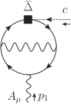
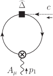
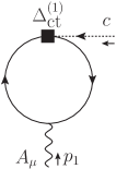
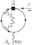
+ loop on the other fermion propagator.

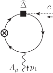
+ fermion counterterm on the other fermion propagator.

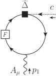
+ fermion finite counterterm on the other fermion propagator.

Figure 4: List of Feynman diagrams for the ghost–photon breaking contribution given in Eq. 7.55.

The total two-loop breaking in this sector, i.e. the result of the diagrams in Fig. 4 is

$$i\left([\widehat{\Delta}+\Delta_{\text{ct}}^{1}]\cdot\widetilde{\Gamma}\right)^{2}_{A_{\mu}c}=\frac{1}{256\pi^{4}}\frac{e^{4}\text{Tr}(\mathcal{Y}_{R}^{4})}{6}\left[\left(\frac{1}{\epsilon^{2}}-\frac{17}{12\epsilon}\right)\hat{p}_{1}^{2}\overline{p}_{1}^{\mu}-\frac{11}{4}\overline{p}_{1}^{2}\overline{p}_{1}^{\mu}+\mathcal{O}(\hat{.})\right]\,.$$ (7.55)

The result contains $1/\epsilon^{2}$ poles and $1/\epsilon$ poles with local, evanescent coefficients and a finite, non-evanescent term.

Like at the one-loop level, we first use the result to check the cancellation of the UV divergences as prescribed by Eq. 6.46. As expected, this cancellation with $s_{D}{S^{2}_{\text{sct}}}$ given in Eq. 7.54 indeed occurs as

$$\Delta_{\text{sct}}^{2}=s_{D}{S^{2}_{\text{sct}}}=-\left([\widehat{\Delta}+\Delta_{\text{ct}}^{1}]\cdot\Gamma\right)^{2}_{\text{div}}\,.$$ (7.56)

The remaining finite part can then be evaluated in strictly 4 dimensions,

$$\begin{split}\Delta_{\text{fct}}^{2}=\;&-\mathop{\text{LIM}}_{D\to 4}\left\{\left([\widehat{\Delta}+\Delta_{\text{ct}}^{(1)}]\cdot{\Gamma}\right)^{(2)}+s_{D}{S^{(2)}_{\text{sct}}}\right\}\\ =&\frac{e^{4}}{256\pi^{4}}\text{Tr}(\mathcal{Y}_{R}^{4})\;s\left(\frac{11}{48}\int d^{4}x\bar{A}_{\mu}\overline{\partial}^{2}\bar{A}^{\mu}\right)+\ldots\,.\end{split}$$ (7.57)

The defining relation for the finite, symmetry-restoring counterterm is then

$$\mathop{\text{LIM}}_{D\to 4}s_{D}S^{2}_{\text{fct}}=-\Delta_{\text{fct}}^{2}\,.$$ (7.58)

From this we reconstruct the corresponding finite counterterm as

$$S^{2}_{\text{fct}}=\left(\frac{\hbar}{16\pi^{2}}\right)^{2}\int d^{4}x\,e^{4}\text{Tr}(\mathcal{Y}_{R}^{4})\frac{11}{48}\bar{A}_{\mu}\overline{\partial}^{2}\bar{A}^{\mu}+\ldots\,.$$ (7.59)

As before we only display terms related to the photon self-energy. Adding this counterterm restores the photon self-energy transversality at the 2-loop level.

At this point the determination of the two-loop counterterms of this sector is complete, and the counterterms of other sectors can be determined analogously. The required computations were the ones of the divergent part of the photon self-energy and of the finite part of the diagrams of Fig. 4.

Nevertheless we now confirm the result by comparing with the explicit result for the finite part of the photon self-energy. The finite part of the photon self-energy at the two-loop level (including one-loop counterterms but excluding two-loop counterterms) is given by

$$\begin{split}\left.i\widetilde{\Gamma}_{AA}^{\mu\nu}(p)\right|^{2}_{\text{fin}}&=\frac{ie^{4}}{256\pi^{4}}\frac{\text{Tr}(\mathcal{Y}_{R}^{4})}{3}\\ &\left[\left(\frac{673}{23}-6\log(-\overline{p}^{2})-24\zeta(3)\right)(\overline{p}^{\mu}\overline{p}^{\nu}-\overline{p}^{2}\overline{g}^{\mu\nu})+\frac{11}{8}\overline{p}^{\mu}\overline{p}^{\nu}\right]\,.\end{split}$$ (7.60)

Similar to the one-loop result (7.35), the non-local $\log(-\overline{p}^{2})$ and transcendental $\zeta(3)$ parts are by themselves transversal and so do not break gauge invariance. The last term breaks the transversality, but this breaking term is local.

Plugging the result into the Ward or Slavnov-Taylor identity we obtain

$$\left.i\,p_{\nu}\,\widetilde{\Gamma}_{A(-p)A(p)}^{\mu\nu}\right|^{2}_{\text{fin}} =\frac{ie^{4}}{256\pi^{4}}\frac{\text{Tr}(\mathcal{Y}_{R}^{4})}{6}\frac{11}{4}\overline{p}^{2}\overline{p}^{\mu}$$ (7.61a)

$$=-\left([\widehat{\Delta}+\Delta_{\text{ct}}^{1}]\cdot\widetilde{\Gamma}\right)^{2}_{\text{fin},\,A_{\mu}(-p)c(p)}\,.$$ (7.61b)

The first of these equations is obtained by direct computation using the finite parts in Eq. (7.60). The second equation is then observed by comparison with Eq. 7.55. Hence we confirm that the violation of the symmetry is restored by our finite counterterm evaluated from breaking diagrams.

7.4.4 Full Two-Loop Renormalization of Chiral QED

In the previous sections we performed the full one-loop renormalization with singular and finite, symmetry-restoring counterterms (7.48) and (7.50), respectively, and studied the photon self-energy and the corresponding breaking at the two-loop level, cf. Sec. 7.4.3. In this section we present the full two-loop renormalization of chiral QED based on our results in Ref. [26].

A list of all divergent 1PI two-loop Green functions together with the individual results is to be found in chapter $7$ of Ref. [26]. From the singular part of these Green functions we obtain the singular counterterm action at the two-loop level

$$S_{\text{sct}}^{2}= -\left(\frac{\hbar e^{2}}{16\pi^{2}}\right)^{2}\frac{\text{Tr}(\mathcal{Y}_{R}^{4})}{3}\bigg{[}\frac{2}{\epsilon}\overline{S_{AA}}+\left(\frac{1}{4\epsilon^{2}}-\frac{17}{48\epsilon}\right)\int d^{D}x\,\bar{A}_{\mu}\widehat{\partial}^{2}\bar{A}^{\mu}\bigg{]}$$

$$+\left(\frac{\hbar e^{2}}{16\pi^{2}}\right)^{2}\sum_{j}(\mathcal{Y}_{R}^{j})^{2}\bigg{[}\left(\frac{1}{2\epsilon^{2}}+\frac{17}{12\epsilon}\right)(\mathcal{Y}_{R}^{j})^{2}-\frac{1}{9\epsilon}\text{Tr}(\mathcal{Y}_{R}^{2})\bigg{]}\left(\overline{S^{j}_{\overline{\psi}\psi_{R}}}+\overline{S^{j}_{\overline{\psi_{R}}A\psi_{R}}}\right)$$

$$-\left(\frac{\hbar e^{2}}{16\pi^{2}}\right)^{2}\sum_{j}\frac{(\mathcal{Y}_{R}^{j})^{2}}{3\epsilon}\bigg{(}\frac{5}{2}(\mathcal{Y}_{R}^{j})^{2}-\frac{2}{3}\text{Tr}(\mathcal{Y}_{R}^{2})\bigg{)}\overline{S^{j}_{\overline{\psi}\psi_{R}}}$$ (7.62)

which cancel the divergences. Comparing (7.4.4) with its one-loop counterpart in Eq. (7.48), we see that its structure is the same up to the term in the last line, which breaks BRST invariance by a non-evanescent amount and is thus a new feature emerging at the two-loop level.

This two-loop counterterm action (7.4.4) generates the BRST breaking

$$\Delta_{\text{sct}}^{2} =s_{D}S_{\text{sct}}^{2}$$

$$=-\frac{\hbar^{2}e^{4}}{256\pi^{4}}\frac{\text{Tr}(\mathcal{Y}_{R}^{4})}{6}\left(\frac{1}{\epsilon^{2}}-\frac{17}{12\epsilon}\right)\int d^{D}x\,(\overline{\partial}_{\mu}c)(\widehat{\partial}^{2}\bar{A}^{\mu})$$ (7.63)

$$\hskip 12.51927pt-\frac{\hbar^{2}e^{5}}{256\pi^{4}}\frac{1}{3\epsilon}\sum_{j}(\mathcal{Y}_{R}^{j})^{3}\bigg{(}\frac{5}{2}(\mathcal{Y}_{R}^{j})^{2}-\frac{2}{3}\text{Tr}(\mathcal{Y}_{R}^{2})\bigg{)}\int d^{D}x\,c\,\overline{\partial}_{\mu}\big{(}\overline{\psi}\bar{\gamma}^{\mu}\mathbb{P}_{R}\psi\big{)}.$$

Compared to the previous section 7.4.3 we this time provided the full two-loop result explicitly and see that, in contrast to the one-loop case (7.40), this BRST breaking contains a non-evanescent contribution given by the last line of (7.4.4).

Following the restoration procedure described in Sections 6.3 or 7.3 and analogous to the ghost–gauge boson contribution (7.55) in the previous Section 7.4.3, we additionally need to calculate $([\widehat{\Delta}+\Delta_{\text{ct}}^{1}]\cdot\widetilde{\Gamma})^{2}$ for the ghost–fermion–fermion, the ghost–double gauge boson, and the ghost–triple gauge boson contributions (i.e. with external fields $c\psi\bar{\psi}$, $cAA$, $cAAA$, respectively). It turns out that the ghost–double gauge boson contribution vanishes and the ghost–triple gauge boson contribution does not contain UV divergences, but only finite terms. In total the result is

$$\left(\big{[}\widehat{\Delta}+\Delta_{\text{ct}}^{1}\big{]}\cdot\Gamma\right)^{2} =\frac{e^{4}}{256\pi^{4}}\int d^{D}x\,$$

$$\bigg{\{}-\frac{\text{Tr}(\mathcal{Y}_{R}^{4})}{6}\bigg{[}\left(\frac{1}{\epsilon^{2}}-\frac{17}{12\epsilon}\right)c\,\overline{\partial}_{\mu}\widehat{\partial}^{2}\bar{A}^{\mu}-\frac{11}{4}c\,\overline{\partial}_{\mu}\overline{\partial}^{2}\bar{A}^{\mu}\bigg{]}$$

$$+e\sum_{j}\frac{(\mathcal{Y}_{R}^{j})^{3}}{3}\bigg{[}\frac{1}{\epsilon}\left(\frac{5}{2}(\mathcal{Y}_{R}^{j})^{2}-\frac{2}{3}\text{Tr}(\mathcal{Y}_{R}^{2})\right)$$ (7.64)

$$\hskip 65.44142pt+\frac{127}{12}(\mathcal{Y}_{R}^{j})^{2}-\frac{1}{9}\text{Tr}(\mathcal{Y}_{R}^{2})\bigg{]}c\,\overline{\partial}_{\mu}\big{(}\overline{\psi}_{j}\bar{\gamma}^{\mu}\mathbb{P}_{R}\psi_{j}\big{)}$$

$$+\frac{3e^{2}\text{Tr}(\mathcal{Y}_{R}^{6})}{2}c\,\overline{\partial}_{\mu}\big{(}\bar{A}^{\mu}\bar{A}_{\nu}\bar{A}^{\nu}\big{)}\bigg{\}}+\mathcal{O}(\hat{.})$$

for the full two-loop breaking of the Slavnov-Taylor identity of two-loop subrenormalized 1PI Green functions. Comparing this with the corresponding one-loop contribution (7.49), we see that the structure of the terms is the same.

For the symmetry restoration at the two-loop level, we first note that $\Delta_{\text{sct}}^{2}$ in Eq. (7.4.4) completely cancels the UV divergent terms in Eq. (7.4.4). In addition to that, we need to determine the finite, symmetry-restoring counterterms at the two-loop as indicated in Eq. (7.57). Thus, our choice for the full finite counterterm action, which restores the Slavnov-Taylor identity at the two-loop level, is

$$S_{\text{fct}}^{2} =\left(\frac{\hbar}{16\pi^{2}}\right)^{2}\int d^{D}x\,e^{4}\bigg{\{}\text{Tr}(\mathcal{Y}_{R}^{4})\frac{11}{48}\bar{A}_{\mu}\overline{\partial}^{2}\bar{A}^{\mu}+3e^{2}\frac{\text{Tr}(\mathcal{Y}_{R}^{6})}{8}\bar{A}_{\mu}\bar{A}^{\mu}\bar{A}_{\nu}\bar{A}^{\nu}$$

$$\hskip 62.59596pt-\sum_{j}(\mathcal{Y}_{R}^{j})^{2}\left(\frac{127}{36}(\mathcal{Y}_{R}^{j})^{2}-\frac{1}{27}\text{Tr}(\mathcal{Y}_{R}^{2})\right)\Big{(}\overline{\psi}_{j}i\bar{\not{\partial}}\mathbb{P}_{R}\psi_{j}\Big{)}\bigg{\}}.$$ (7.65)

Similar to its one-loop counterpart in Eq. (7.50), $S_{\text{fct}}^{2}$ consists of three kinds of terms, or in other words, the same three field monomials are involved. These three terms correspond to the restoration of the Ward identity relations for the photon self-energy, the photon $4$-point function and the fermion self-energy/photon-fermion-fermion interaction. Ref. [26] also gave a discussion of the explicit results for these three Ward identity relations, similar to the discussion at the end of Sec. 7.4.3. In all cases, the breaking terms of the Ward identity are explicitly exhibited and the cancellation with the symmetry-restoring counterterms (7.4.4) is made manifest.

7.5 Non-Abelian Chiral Yang-Mills Theory and Comparison with the Abelian Chiral Theory at the One-Loop Level

In this section we review the application of the BMHV scheme to non-abelian chiral gauge theories and present the differences to the abelian chiral QED discussed above. In particular, we study a massless chiral Yang-Mills theory at the one-loop level based on Refs. [25, 131]. Note that in our publication [25] the considered theory also contained real scalar fields. Here, similar to Ref. [131], scalar fields are omitted in order to focus on the key-points of the BMHV scheme in the framework of chiral gauge theories and the differences compared to the abelian case discussed above.

As discussed in section 2.1, the group generators of Yang-Mills theories satisfy the non-trivial commutation relations (2.1); in particular, they are not simultaneously diagonalizable. These algebraic structures of the non-Abelian gauge group of Yang-Mills theories lead to new effects, such as more interactions terms and non-linear BRST transformations of the gauge fields and the ghosts, compared to the Abelian case, cf. Sec. 2.6. Especially, gauge boson self-interactions, interactions of the Faddeev-Popov ghosts with the rest of the theory and the renormalization of the BRST transformations distinguish non-Abelian Yang-Mills theories from the Abelian case above.

The outline of this section is analogous to the Abelian case discussed above. First, we briefly introduce the Lagrangian of the theory and the BRST transformations using the notations from section 2. Second, we discuss the analytical continuation of the theory to $D$ dimensions in DReg treating $\gamma_{5}$ with the BMHV scheme and comment on the BRST breaking induced by this scheme. Finally, we present the results for the singular and the symmetry restoring counterterms at the one-loop level, cf. [25, 131], necessary to consistently renormalize the theory, and discuss the differences to the Abelian theory.

7.5.1 Definition of the Non-Abelian Chiral Yang–Mills Theory

Following the conventions of Sec. 2.3, the Lagrangian in $4$ dimensions can be written as

$${\cal L}_{\chi\text{YM}}={\cal L}_{\text{inv}}+{\cal L}_{\text{fix,gh}}+{\cal L}_{\text{ext}}\,.$$ (7.66)

The physical part of the Yang-Mills Lagrangian reads

$${\cal L}_{\text{inv}}=-\frac{1}{4}G^{a}_{\mu\nu}G^{a,\mu\nu}+i\,\overline{\psi_{R}}_{i}\not{D}_{ij}{\psi_{R}}_{j}\,,$$ (7.67)

with covariant derivative $D^{\mu}_{ij}=\partial^{\mu}\delta_{ij}+igG^{a,\mu}\,{T^{a}_{R}}_{ij}$ and field strength tensor $G^{a}_{\mu\nu}=\partial_{\mu}G^{a}_{\nu}-\partial_{\nu}G^{a}_{\mu}-gf^{abc}G^{b}_{\mu}G^{c}_{\nu}$, leading to three- and four-point gauge boson self-interactions. The gauge-fixing and ghost Lagrangian, already presented in Eq. (2.65), is

$${\cal L}_{\text{fix,gh}}=s\left[\bar{c}^{a}\left((\partial^{\mu}G^{a}_{\mu})+\frac{\xi}{2}B^{a}\right)\right]=B^{a}(\partial^{\mu}G^{a}_{\mu})+\frac{\xi}{2}B^{a}B^{a}-\bar{c}^{a}\partial^{\mu}D^{ab}_{\mu}c^{b},$$ (7.68)

with $D^{ab}_{\mu}=\partial_{\mu}\delta^{ab}+gf^{abc}G_{\mu}^{c}$, implying ghost-antighost-gauge boson interactions which is a consequence of the nonlinear gauge transformations of the gauge fields $G^{a}_{\mu}$ as shown below in (7.70). The Lagrangian of the external sources, as introduced in Sec. 2.3, is

$${\cal L}_{\text{ext}}=\rho^{a,\mu}sG_{\mu}^{a}+\zeta^{a}sc^{a}+\bar{R}^{i}s{\psi_{R}}_{i}+R^{i}s\overline{\psi_{R}}_{i}\,.$$ (7.69)

The BRST transformations are given by

$$sG^{a}_{\mu}(x) =D_{\mu}^{ab}c^{b}(x)=\partial_{\mu}c^{a}(x)+gf^{abc}c^{b}(x)G^{c}_{\mu}(x)\,,$$ (7.70a)

$$s\psi_{i}(x) =s{\psi_{R}}_{i}(x)=-ig{T^{a}_{R}}_{ij}c^{a}(x){\psi_{R}}_{j}(x)\,,$$ (7.70b)

$$s\overline{\psi}_{i}(x) =s\overline{\psi_{R}}_{i}(x)=-ig\overline{\psi_{R}}_{j}(x)c^{a}(x){T^{a}_{R}}_{ji}\,,$$ (7.70c)

$$sc^{a}(x) =\frac{1}{2}gf^{abc}c^{b}(x)c^{c}(x)\,,$$ (7.70d)

$$s\bar{c}^{a}(x) =B^{a}(x)\,,$$ (7.70e)

$$sB^{a}(x) =0\,.$$ (7.70f)

In contrast to the Abelian case, the BRST transformations of the gauge boson $G^{a}_{\mu}$ and the Faddeev-Popov ghost $c^{a}$ are non-linear, which means that non-trivial quantum corrections are expected.

Hence, the tree-level action of the considered chiral Yang-Mills theory in $4$ dimensions is given by

$$S_{0}^{(4D)}=\int d^{4}x\,{\cal L}_{\chi\text{YM}}$$ (7.71)

and satisfies the tree-level Slavnov-Taylor identity

$$0 =\mathcal{S}\big{(}S_{0}^{(4D)}\big{)}$$

$$=\int d^{4}x\Bigg{(}\frac{\delta S_{0}^{(4D)}}{\delta\rho^{a}{}^{\mu}(x)}\frac{\delta S_{0}^{(4D)}}{\delta G^{a}_{\mu}(x)}+\frac{\delta S_{0}^{(4D)}}{\delta\zeta^{a}(x)}\frac{\delta S_{0}^{(4D)}}{\delta c^{a}(x)}$$ (7.72)

$$\hskip 41.25641pt+\frac{\delta S_{0}^{(4D)}}{\delta\bar{R}^{i}(x)}\frac{\delta S_{0}^{(4D)}}{\delta{\psi_{R}}_{i}(x)}+\frac{\delta S_{0}^{(4D)}}{\delta{R}^{i}(x)}\frac{\delta S_{0}^{(4D)}}{\delta\overline{\psi_{R}}_{i}(x)}+B^{a}(x)\frac{\delta S_{0}^{(4D)}}{\delta\bar{c}^{a}(x)}\Bigg{)},$$

which just manifests the BRST invariance of $S_{0}^{(4D)}$.

The different group invariants, which will be employed in the following results below, follow the notations of [25] and are provided by

$$C_{2}(R)\,\mathbbm{1} =T^{a}_{R}T^{a}_{R}\,, S_{2}(R)\,\delta^{ab} =\text{Tr}\big{(}T^{a}_{R}T^{b}_{R}\big{)},$$ (7.73)

with an irreducible representation $R$ of the gauge group for the right-handed fermions with corresponding Hermitian group generators $T^{a}_{R}$. The adjoint representation of the gauge group is denoted by $G$ and its Casimir index is $C_{2}(G)$.

7.5.2 Chiral Yang–Mills Theory in DReg

To regularize the theory we employ dimensional regularization, treating $\gamma_{5}$ with the BMHV scheme. Analogous to the Abelian case above, there are two problems regarding the continuation of the chiral Yang-Mills theory (7.71) to $D$ dimensions, as already discussed in Sec. 7.2.2 for the Abelian case and extensively discussed in [25] for chiral Yang-Mills theories.

First, there is an ambiguity in extending the fermion-gauge interaction term in Eq. (7.67), which involves the right-handed chiral current $\overline{\psi_{R}}_{i}\gamma^{\mu}{\psi_{R}}_{j}$, to $D$ dimensions. Again, there are three inequivalent choices for the $D$-dimensional version of this chiral current, cf. Eq. (7.12), which are all equally correct. Analogous to the Abelian case above, we resolve this problem by choosing the most symmetric version cf. Eq. (7.13).

Second, the purely fermionic kinetic term $i\overline{\psi_{R}}_{i}\not{\partial}{\psi_{R}}_{i}$ projects only the purely $4$-dimensional derivative, leading to a purely $4$-dimensional propagator and thus to unregularized loop diagrams, as explained above in Sec. 7.2.2. Hence, we again introduce a gauge-singlet left-chiral field $\psi_{L}$ with trivial BRST transformations

$$s{\psi_{L}}_{i}(x) =0, s\overline{\psi_{L}}_{i}(x) =0,$$ (7.74)

which appears solely in the fermionic kinetic term and nowhere else and which is thus completely decoupled from the rest of the theory. Using it we obtain a fully $D$-dimensional covariant kinetic term $i\overline{\psi}_{i}\not{\partial}\psi_{i}$.

Finally, we can again separate the $D$-dimensional fermionic Lagrangian into an invariant and an evanescent part, analogous to Eqs. (7.17a) to (7.20b). Hence, we may write the $D$-dimensional action as

$$S_{0} =S_{0,\text{inv}}+S_{0,\text{evan}}$$

$$=(S_{GG}+S_{GGG}+S_{GGGG})+\sum_{i}\left(S^{i}_{\overline{\psi}\psi}+\overline{S^{i}_{\overline{\psi}_{R}G\psi_{R}}}\right)+S_{\text{g-fix}}$$ (7.75)

$$\hskip 12.51927pt+(S_{\bar{c}c}+S_{\bar{c}Gc})+(S_{\rho c}+S_{\rho Gc}+S_{\zeta cc}+S_{\bar{R}c\psi_{R}}+S_{Rc\overline{\psi_{R}}})\,,$$

having it separated into an “invariant” and an “evanescent” part in the first line, cf. Eq. (7.22) in Sec. 7.2.2, and having used the notation of [26, 25] and of Eq. (7.21) to present the $D$-dimensional action as a sum of its integrated field monomials in the last two lines.

Similar to the Abelian case in Sec. 7.2.2, we quantify the symmetry breaking caused by the BMHV scheme, the non-anticommuting $\gamma_{5}$ and the evanescent term $S_{0,\text{evan}}$ by acting with the $D$-dimensional BRST operator $s_{D}$ on the $D$-dimensional tree-level action $S_{0}$. Thus, for the BRST breaking we obtain

$$s_{D}S_{0}=s_{D}S_{0,\text{inv}}+s_{D}S_{0,\text{evan}}=0+s_{D}\int d^{D}x\,i\overline{\psi}_{i}\widehat{\not{\partial}}{\psi}_{i}\equiv\widehat{\Delta}\,,$$ (7.76)

which leads to a breaking of the Slavnov-Taylor identity of the form

$$\mathcal{S}_{D}\big{(}S_{0}\big{)} =\widehat{\Delta}\,,$$ (7.77)

with the non-vanishing integrated breaking

$$\widehat{\Delta}=-\int d^{D}xg\,{T^{a}_{R}}_{ij}\,c^{a}\,\left\{\overline{\psi}_{i}\left(\overset{\leftarrow}{\widehat{\not{\partial}}}\mathbb{P}_{R}+\overset{\rightarrow}{\widehat{\not{\partial}}}\mathbb{P}_{L}\right)\psi_{j}\right\}\equiv\int d^{D}x\,\widehat{\Delta}(x).$$ (7.78)

As in the Abelian case, this breaking term will be a crucial tool in practical calculations and will be used as a composite operator insertion in Feynman diagrams. It generates an interaction vertex whose Feynman rule (with all momenta incoming) is:

$$\begin{aligned} &=-\frac{g}{2}\,{T^{a}_{R}}_{ij}\left((\widehat{\not{p_{1}}}+\widehat{\not{p_{2}}})+(\widehat{\not{p_{1}}}-\widehat{\not{p_{2}}})\gamma_{5}\right)_{\alpha\beta}\\ &=-g\,{T^{a}_{R}}_{ij}\left(\widehat{\not{p_{1}}}\mathbb{P}_{R}+\widehat{\not{p_{2}}}\mathbb{P}_{L}\right)_{\alpha\beta}\,.\end{aligned}$$

(7.79)

For charge-conjugated fermions an analogous Feynman rule can be derived.

7.5.3 One-Loop Singular Counterterm and Symmetry-Restoring Counterterm Action in Chiral Yang–Mills Theory

In this subsection, we present the results of the one-loop renormalization of the above introduced chiral Yang-Mills theory based on the results of [25], but also already discussed in [131].

The basic renormalization procedure is the same as in the Abelian theory discussed above. The difference is that there are more interaction terms; in particular, the gauge bosons interact with themselves and with the Faddeev-Popov ghosts. The fact that the ghosts now participate in interactions, and thus may propagate as internal particles in loop diagrams, leads to a non-trivial renormalization of the field monomials including external sources. Besides this, the renormalization procedure is also more demanding than in an Abelian theory, due to the larger number of loop diagrams and the more complicated algebraic structures of the non-Abelian gauge group.

After computing all UV divergent one-loop 1PI Feynman diagrams, which can be found in section $5$ of [25] with detailed individual results, the singular one-loop counterterm action is given by

$$S_{\text{sct}}^{(1)} =\frac{\hbar g^{2}}{16\pi^{2}\epsilon}\bigg{\{}-\frac{2S_{2}(R)}{3}\big{(}\overline{S_{GG}}+\overline{S_{GGG}}+\overline{S_{GGGG}}\big{)}-\xi C_{2}(R)\big{(}\overline{S_{\overline{\psi}\psi_{R}}}+\overline{S_{\overline{\psi}G\psi_{R}}}\big{)}$$

$$\hskip 14.22636pt+\frac{13-3\xi}{6}C_{2}(G)S_{GG}+\frac{17-9\xi}{12}C_{2}(G)S_{GGG}+\frac{2-3\xi}{3}C_{2}(G)S_{GGGG}$$

$$\hskip 14.22636pt-\frac{3+\xi}{4}C_{2}(G)\overline{S_{\overline{\psi}G\psi_{R}}}+\frac{3-\xi}{4}C_{2}(G)\big{(}S_{\bar{c}c}+S_{\rho c}\big{)}$$ (7.80)

$$\hskip 14.22636pt-\frac{\xi C_{2}(G)}{2}\big{(}S_{\bar{c}Gc}+S_{\rho Gc}+S_{\zeta cc}+S_{\bar{R}c\psi_{R}}+S_{Rc\overline{\psi_{R}}}\big{)}\bigg{\}}$$

$$\hskip 14.22636pt-\frac{\hbar g^{2}}{16\pi^{2}\epsilon}\frac{S_{2}(R)}{3}\int d^{4}x\,\frac{1}{2}\bar{G}^{a,\mu}\widehat{\partial}^{2}\bar{G}^{a}_{\mu},$$

such that it cancels all UV-divergences. The structure has similarities with the Abelian counterpart, Eq. (7.48). Again, most terms can be obtained by a renormalization transformation of the kind (6.3), and only the right-handed fermions renormalize. But again also non-symmetric singular counterterms appear.

Comparing Eqs. (7.5.3) and (7.48) in detail, we can see many additional contributions. Only the $\overline{S_{GG}}$, $\overline{S_{\overline{\psi}\psi_{R}}}$ and $\overline{S_{\overline{\psi}G\psi_{R}}}$ terms in the first line of the RHS of (7.5.3) as well as the explicit evanescent operator in last line of (7.5.3) have Abelian counterparts. All other terms in (7.5.3) do not appear in the Abelian theory, and are thus new effects of the non-Abelian Yang-Mills theory due to additional interaction terms, as mentioned above. In particular, we can see new contributions to the field monomials including the Faddeev-Popov ghosts and the external sources in the last term of the third line and the penultimate line of (7.5.3), as announced at the beginning of this subsection.

Similar to the Abelian result (7.48), we have just one explicit evanescent operator in the last line of (7.5.3) in the considered Yang-Mills theory, generating the Feynman rule $-i\widehat{p}^{2}\overline{g}_{\mu\nu}\delta^{ab}$. This is specific to our choice for the fermion-gauge interaction term, corresponding to the most symmetric version of Eq. (7.13). We would have obtained many more evanescent operators, if we used another $D$-dimensional choice instead.

Following the algebraic renormalization procedure described in section 6, as well as in section $6$ of [25] specifically for the considered case, we need to check that

$$0=\mathop{\text{LIM}}_{D\,\to\,4}\,\bigg{(}\big{[}\widehat{\Delta}\cdot\Gamma^{(1)}\big{]}_{\text{div}}^{(1)}+b_{D}S_{\text{sct}}^{(1)}+\big{[}\widehat{\Delta}\cdot\Gamma^{(1)}\big{]}_{\text{fin}}^{(1)}+b_{D}S_{\text{fct,restore}}^{(1)}\bigg{)}.$$ (7.81)

In other words, we need to check that the $b_{D}$-variation of the singular counterterms (7.5.3) cancels the divergent part of the symmetry breaking $[\widehat{\Delta}\cdot\Gamma^{(1)}]_{\text{div}}^{(1)}$ and we need to determine finite symmetry-restoring counterterms $S_{\text{fct,restore}}^{(1)}$ whose $b_{D}$-variation cancel the finite part of the symmetry breaking $[\widehat{\Delta}\cdot\Gamma^{(1)}]_{\text{fin}}^{(1)}$.

The $b_{D}$-variation of the singular counterterms (7.5.3), calculated in [25], is provided by

$$b_{D}S_{\text{sct}}^{(1)}=\frac{-\hbar}{16\pi^{2}\epsilon}\bigg{\{}g^{2}\frac{\xi C_{2}(G)}{2}\widehat{\Delta}+g^{2}\frac{S_{2}(R)}{3}b_{D}\int d^{D}x\,\frac{1}{2}\bar{G}^{a,\mu}\widehat{\partial}^{2}\bar{G}^{a}_{\mu}\bigg{\}},$$ (7.82)

where, in the last term, $b_{D}$ acts like the BRST transformation, leading to

$$b_{D}\int d^{D}x\,\frac{1}{2}\bar{G}^{a,\mu}\widehat{\partial}^{2}\bar{G}^{a}_{\mu} =\int d^{D}x\,\big{(}s_{D}\bar{G}^{a,\mu}\big{)}\widehat{\partial}^{2}\bar{G}^{a}_{\mu}$$

$$=\int d^{D}x\,\Big{(}\overline{\partial}^{\mu}c^{a}-gf^{abc}\bar{G}^{b,\mu}c^{c}\Big{)}\widehat{\partial}^{2}\bar{G}^{a}_{\mu}\,.$$ (7.83)

Indeed, (7.82) is a pure $1/\epsilon$ singular term and perfectly cancels the non-vanishing contribution

$$\big{[}\widehat{\Delta}\cdot\Gamma\big{]}_{\text{div}}^{(1)}=\frac{1}{16\pi^{2}\epsilon}\bigg{\{}g^{2}\frac{\xi C_{2}(G)}{2}\widehat{\Delta}+g^{2}\frac{S_{2}(R)}{3}\int d^{D}x\,\Big{(}\overline{\partial}^{\mu}c^{a}-gf^{abc}\bar{G}^{b,\mu}c^{c}\Big{)}\widehat{\partial}^{2}\bar{G}^{a}_{\mu}\bigg{\}},$$ (7.84)

as explicitly shown in [25].

Now, the finite symmetry-restoring counterterms $S_{\text{fct,restore}}^{(1)}$ need to be determined following (7.81) in order to cancel the remaining finite part of the symmetry breaking, which was explicitly performed in section $6$ of [25] with the result

$$S_{\text{fct, restore}}^{(1)} =\frac{\hbar}{16\pi^{2}}\bigg{\{}g^{2}\frac{S_{2}(R)}{6}\bigg{(}5S_{GG}-\int d^{4}x\,G^{a,\mu}\partial^{2}G^{a}_{\mu}\bigg{)}$$

$$\hskip 12.51927pt+g^{2}\frac{(T_{R})^{abcd}}{3}\int d^{4}x\,\frac{g^{2}}{4}G^{a}_{\mu}G^{b,\mu}G^{c}_{\nu}G^{d,\nu}+g^{2}\bigg{(}1+\frac{\xi-1}{6}\bigg{)}C_{2}(R)S_{\overline{\psi}\psi}$$

$$\hskip 12.51927pt+g^{2}\frac{S_{2}(R)}{6}S_{GGG}-g^{2}\frac{\xi C_{2}(G)}{4}\big{(}S_{\bar{R}c\psi_{R}}+S_{Rc\overline{\psi_{R}}}\big{)}\bigg{\}},$$ (7.85)

where $(T_{R})^{a_{1}\cdots a_{n}}\equiv\text{Tr}[T^{a_{1}}_{R}\cdots T^{a_{n}}_{R}]$. Comparing (7.85) with the Abelian result (7.50), we can again see that only the first two lines of (7.85) have Abelian counterparts, whereas the terms in the last line of (7.85) do not appear in an Abelian theory. The new terms in the last line of (7.85) are due to triple gauge boson contributions and contributions including external sources. The latter implies that again Green functions with external sources have to been evaluated, this time with a $\widehat{\Delta}$-vertex insertion, which stands in contrast to the Abelian case.

These finite counterterms (7.85) are necessary and sufficient to restore the BRST symmetry at the one-loop level in the BMHV scheme, if the (non-spurious) anomalies cancel, which are given by [25]

$$-\frac{g^{2}}{16\pi^{2}}\bigg{(}-\frac{S_{2}(R)}{3}d_{R}^{abc}\int d^{4}x\,g\epsilon^{\mu\nu\rho\sigma}c^{a}\big{(}\partial_{\rho}G^{b}_{\mu}\big{)}\big{(}\partial_{\sigma}G^{c}_{\nu}\big{)}$$

$$\hskip 68.28644pt+\frac{\mathcal{D}_{R}^{abcd}}{3\times 3!}\int d^{4}x\,g^{2}c^{a}\epsilon^{\mu\nu\rho\sigma}\partial_{\sigma}\Big{(}G^{b}_{\mu}G^{c}_{\nu}G^{d}_{\rho}\Big{)}\bigg{)},$$ (7.86)

with fully symmetric $d_{R}^{abc}\equiv\text{Tr}[T_{R}^{a}\{T_{R}^{b},T_{R}^{c}\}]$ and fully antisymmetric $\mathcal{D}_{R}^{abcd}\equiv(-i)3!\text{Tr}[T_{R}^{a}T_{R}^{[b}T_{R}^{c}T_{R}^{d]}]$ for the $R$-representation. This result of course agrees with the general result (6.30) obtained by the analysis of algebraic renormalization, and it provides an explicit result for the coefficient $L$ appearing there. To ensure the renormalizability of the theory the fermionic content and their associated group representations have to be chosen such that these anomalies cancel, i.e. such that the expression (6.33) vanishes, which equivalently means that $d_{R}^{abc}$ vanishes. This then also implies the vanishing of $\mathcal{D}_{R}^{abcd}$, see Eq. (6.32). It becomes apparent that also the possible anomalies are more complex than in the Abelian model.

These finite counterterms (7.85), purely $4$-dimensional and non-evanescent, are not gauge-invariant. They modify all self-energies, as well as some specific interactions: the gauge-boson self-interactions and the interactions between gauge-bosons and fermions.

Concluding, we see that the resulting counterterm action, not only for the Abelian case at the one- and two-loop level, but also for non-Abelian Yang-Mills theories, may be written in a relatively compact way. Thus, treating $\gamma_{5}$ rigorously in the BMHV scheme does not lead to extraordinarily lengthy or complicated results, but in fact to counterterms which can easily be implemented in computer algebra systems.

8 Acknowledgments

A.I., H.B. and M.M. acknowledge financial support from the Croatian Science Foundation (HRZZ) under the project “PRECIOUS” (“Precise Computations of Physical Observables in Supersymmetric Models”) number HRZZ-IP-2016-06-7460. P.K., D.S. and M.W. acknowledge financial support by the German Science Foundation DFG, grant STO 876/8-1.

References

- [1] G. ’t Hooft and M. J. G. Veltman, “Regularization and Renormalization of Gauge Fields,” Nucl. Phys. B, vol. 44, pp. 189–213, 1972.
- [2] C. G. Bollini and J. J. Giambiagi, “Dimensional Renormalization: The Number of Dimensions as a Regularizing Parameter,” Nuovo Cim. B, vol. 12, pp. 20–26, 1972.
- [3] J. F. Ashmore, “A Method of Gauge Invariant Regularization,” Lett. Nuovo Cim., vol. 4, pp. 289–290, 1972.
- [4] P. Breitenlohner and D. Maison, “Dimensional Renormalization and the Action Principle,” Commun. Math. Phys., vol. 52, pp. 11–38, 1977.
- [5] C. Gnendiger et al., “To , or not to : recent developments and comparisons of regularization schemes,” Eur. Phys. J. C, vol. 77, no. 7, p. 471, 2017.
- [6] S. L. Adler, “Axial vector vertex in spinor electrodynamics,” Phys. Rev., vol. 177, pp. 2426–2438, 1969.
- [7] J. S. Bell and R. Jackiw, “A PCAC puzzle: in the model,” Nuovo Cim. A, vol. 60, pp. 47–61, 1969.
- [8] S. L. Adler and W. A. Bardeen, “Absence of higher order corrections in the anomalous axial vector divergence equation,” Phys. Rev., vol. 182, pp. 1517–1536, 1969.
- [9] C. Bouchiat, J. Iliopoulos, and P. Meyer, “An Anomaly Free Version of Weinberg’s Model,” Phys. Lett. B, vol. 38, pp. 519–523, 1972.
- [10] D. J. Gross and R. Jackiw, “Effect of anomalies on quasirenormalizable theories,” Phys. Rev. D, vol. 6, pp. 477–493, 1972.
- [11] C. Q. Geng and R. E. Marshak, “Uniqueness of Quark and Lepton Representations in the Standard Model From the Anomalies Viewpoint,” Phys. Rev. D, vol. 39, p. 693, 1989.
- [12] K. Fujikawa, “Path Integral Measure for Gauge Invariant Fermion Theories,” Phys. Rev. Lett., vol. 42, pp. 1195–1198, 1979.
- [13] K. Fujikawa, “Path Integral for Gauge Theories with Fermions,” Phys. Rev. D, vol. 21, p. 2848, 1980. [Erratum: Phys.Rev.D 22, 1499 (1980)].
- [14] M. S. Chanowitz, M. Furman, and I. Hinchliffe, “The Axial Current in Dimensional Regularization,” Nucl. Phys. B, vol. 159, pp. 225–243, 1979.
- [15] F. Jegerlehner, “Facts of life with gamma(5),” Eur. Phys. J. C, vol. 18, pp. 673–679, 2001.
- [16] D. Kreimer, “The (5) Problem and Anomalies: A Clifford Algebra Approach,” Phys. Lett. B, vol. 237, pp. 59–62, 1990.
- [17] J. G. Korner, D. Kreimer, and K. Schilcher, “A Practicable gamma(5) scheme in dimensional regularization,” Z. Phys. C, vol. 54, pp. 503–512, 1992.
- [18] D. Kreimer, “The Role of gamma(5) in dimensional regularization,” 12 1993.
- [19] G. M. Cicuta and E. Montaldi, “Analytic renormalization via continuous space dimension,” Lett. Nuovo Cim., vol. 4, pp. 329–332, 1972.
- [20] D. A. Akyeampong and R. Delbourgo, “Dimensional regularization and PCAC,” Nuovo Cim. A, vol. 18, pp. 94–104, 1973.
- [21] D. A. Akyeampong and R. Delbourgo, “Dimensional regularization, abnormal amplitudes and anomalies,” Nuovo Cim. A, vol. 17, pp. 578–586, 1973.
- [22] E. R. Speer, “Renormalization and ward identities using complex space-time dimension,” J. Math. Phys., vol. 15, pp. 1–6, 1974.
- [23] P. Breitenlohner and D. Maison, “Dimensionally Renormalized Green’s Functions for Theories with Massless Particles. 1.,” Commun. Math. Phys., vol. 52, p. 39, 1977.
- [24] P. Breitenlohner and D. Maison, “Dimensionally Renormalized Green’s Functions for Theories with Massless Particles. 2.,” Commun. Math. Phys., vol. 52, p. 55, 1977.
- [25] H. Bélusca-Maïto, A. Ilakovac, M. Mađor-Božinović, and D. Stöckinger, “Dimensional regularization and Breitenlohner-Maison/’t Hooft-Veltman scheme for applied to chiral YM theories: full one-loop counterterm and RGE structure,” JHEP, vol. 08, no. 08, p. 024, 2020.
- [26] H. Bélusca-Maïto, A. Ilakovac, P. Kühler, M. Mađor-Božinović, and D. Stöckinger, “Two-loop application of the Breitenlohner-Maison/’t Hooft-Veltman scheme with non-anticommuting 5: full renormalization and symmetry-restoring counterterms in an abelian chiral gauge theory,” JHEP, vol. 11, p. 159, 2021.
- [27] C. Cornella, F. Feruglio, and L. Vecchi, “Gauge Invariance and Finite Counterterms in Chiral Gauge Theories,” 5 2022.
- [28] H. Bélusca-Maïto, “Renormalisation Group Equations for BRST-Restored Chiral Theory in Dimensional Renormalisation: Application to Two-Loop Chiral-QED,” 8 2022.
- [29] H. Bélusca-Maïto, A. Ilakovac, M. Mađor-Božinović, P. Kühler, and D. Stöckinger, “Gamma5 in dimensional regularization - a no-compromise approach using the BMHV scheme,” PoS, vol. LL2022, p. 011, 2022.
- [30] T. P. Cheng and L. F. Li, Gauge theory of elementary particle physics. Oxford, UK: Oxford University Press, 1984.
- [31] S. Weinberg, The Quantum theory of fields. Vol. 1: Foundations. Cambridge University Press, 6 2005.
- [32] S. Weinberg, The quantum theory of fields. Vol. 2: Modern applications. Cambridge University Press, 8 2013.
- [33] M. E. Peskin and D. V. Schroeder, An Introduction to quantum field theory. Reading, USA: Addison-Wesley, 1995.
- [34] M. Bohm, A. Denner, and H. Joos, Gauge theories of the strong and electroweak interaction. 2001.
- [35] M. Srednicki, Quantum field theory. Cambridge University Press, 1 2007.
- [36] M. D. Schwartz, Quantum Field Theory and the Standard Model. Cambridge University Press, 2018, 10th printing.
- [37] E. P. Wigner, “On Unitary Representations of the Inhomogeneous Lorentz Group,” Annals Math., vol. 40, pp. 149–204, 1939.
- [38] L. H. Ryder, QUANTUM FIELD THEORY. Cambridge University Press, 6 1996.
- [39] H. K. Dreiner, H. E. Haber, and S. P. Martin, “Two-component spinor techniques and Feynman rules for quantum field theory and supersymmetry,” Phys. Rept., vol. 494, pp. 1–196, 2010.
- [40] L. D. Faddeev and V. N. Popov, “Feynman Diagrams for the Yang-Mills Field,” Phys. Lett. B, vol. 25, pp. 29–30, 1967.
- [41] C. Becchi, A. Rouet, and R. Stora, “The Abelian Higgs-Kibble Model. Unitarity of the S Operator,” Phys. Lett. B, vol. 52, pp. 344–346, 1974.
- [42] C. Becchi, A. Rouet, and R. Stora, “Renormalization of the Abelian Higgs-Kibble Model,” Commun. Math. Phys., vol. 42, pp. 127–162, 1975.
- [43] C. Becchi, A. Rouet, and R. Stora, “Renormalization of Gauge Theories,” Annals Phys., vol. 98, pp. 287–321, 1976.
- [44] I. V. Tyutin, “Gauge Invariance in Field Theory and Statistical Physics in Operator Formalism,” 1975.
- [45] T. Kugo and I. Ojima, “Local Covariant Operator Formalism of Nonabelian Gauge Theories and Quark Confinement Problem,” Prog. Theor. Phys. Suppl., vol. 66, pp. 1–130, 1979.
- [46] M. Henneaux and C. Teitelboim, Quantization of gauge systems. 1992.
- [47] O. Piguet and S. P. Sorella, Algebraic renormalization: Perturbative renormalization, symmetries and anomalies, vol. 28. 1995.
- [48] A. Denner, G. Weiglein, and S. Dittmaier, “Application of the background field method to the electroweak standard model,” Nucl. Phys. B, vol. 440, pp. 95–128, 1995.
- [49] A. Duncan, The Conceptual Framework of Quantum Field Theory. Oxford University Press, 8 2012.
- [50] J. Zinn-Justin, Quantum field theory and critical phenomena, vol. 77 of International Series of Monographs on Physics. Oxford University Press, 4 2021.
- [51] C. Itzykson and J. B. Zuber, Quantum Field Theory. International Series In Pure and Applied Physics, New York: McGraw-Hill, 1980.
- [52] L. S. Brown, Quantum Field Theory. Cambridge University Press, 1992.
- [53] E. Kraus and K. Sibold, “Rigid invariance as derived from BRS invariance: The Abelian Higgs model,” Z. Phys. C, vol. 68, pp. 331–344, 1995.
- [54] R. Haussling and E. Kraus, “Gauge parameter dependence and gauge invariance in the Abelian Higgs model,” Z. Phys. C, vol. 75, pp. 739–750, 1997.
- [55] R. Haussling, E. Kraus, and K. Sibold, “Gauge parameter dependence in the background field gauge and the construction of an invariant charge,” Nucl. Phys. B, vol. 539, pp. 691–719, 1999.
- [56] P. A. Grassi, “The Abelian anti-ghost equation for the standard model in the ’t Hooft background gauge,” Nucl. Phys. B, vol. 537, pp. 527–548, 1999.
- [57] E. Kraus, “Renormalization of the Electroweak Standard Model to All Orders,” Annals Phys., vol. 262, pp. 155–259, 1998.
- [58] P. A. Grassi, “Renormalization of nonsemisimple gauge models with the background field method,” Nucl. Phys. B, vol. 560, pp. 499–550, 1999.
- [59] W. Hollik, E. Kraus, M. Roth, C. Rupp, K. Sibold, and D. Stockinger, “Renormalization of the minimal supersymmetric standard model,” Nucl. Phys. B, vol. 639, pp. 3–65, 2002.
- [60] M. Bohm, H. Spiesberger, and W. Hollik, “On the One Loop Renormalization of the Electroweak Standard Model and Its Application to Leptonic Processes,” Fortsch. Phys., vol. 34, pp. 687–751, 1986.
- [61] K. G. Wilson, “Quantum field theory models in less than four-dimensions,” Phys. Rev. D, vol. 7, pp. 2911–2926, 1973.
- [62] E. R. Speer and M. J. Westwater, “GENERIC FEYNMAN AMPLITUDES,” 6 1970.
- [63] J. C. Collins, Renormalization: An Introduction to Renormalization, the Renormalization Group and the Operator-Product Expansion. Cambridge Monographs on Mathematical Physics, Cambridge University Press, 1984.
- [64] V. A. Smirnov, “Evaluating Feynman integrals,” Springer Tracts Mod. Phys., vol. 211, pp. 1–244, 2004.
- [65] K. Hepp, “Proof of the Bogolyubov-Parasiuk theorem on renormalization,” Commun. Math. Phys., vol. 2, pp. 301–326, 1966.
- [66] S. A. Anikin, M. K. Polivanov, and O. I. Zavyalov, “SIMPLE PROOF OF THE BOGOLYUBOV-PARASIUK THEOREM,” Theor. Math. Phys., vol. 17, p. 1082, 1973.
- [67] M. C. Bergere and J. B. Zuber, “Renormalization of feynman amplitudes and parametric integral representation,” Commun. Math. Phys., vol. 35, pp. 113–140, 1974.
- [68] E. R. Speer, “On the structure of analytic renormalization,” Commun. Math. Phys., vol. 23, pp. 23–36, 1971. [Erratum: Commun.Math.Phys. 25, 336 (1972)].
- [69] N. Nakanishi, Graph Theory and Feynman Integrals. Mathematics and its applications : a series of monographs and texts, Gordon and Breach, 1971.
- [70] S. A. Larin, “The Renormalization of the axial anomaly in dimensional regularization,” Phys. Lett. B, vol. 303, pp. 113–118, 1993.
- [71] T. L. Trueman, “Spurious anomalies in dimensional renormalization,” Z. Phys. C, vol. 69, pp. 525–536, 1996.
- [72] K. G. Chetyrkin, M. Misiak, and M. Munz, “ nonleptonic effective Hamiltonian in a simpler scheme,” Nucl. Phys. B, vol. 520, pp. 279–297, 1998.
- [73] G. Bonneau, “Trace and Axial Anomalies in Dimensional Renormalization Through Zimmermann Like Identities,” Nucl. Phys. B, vol. 171, pp. 477–508, 1980.
- [74] G. Bonneau, “ZIMMERMANN IDENTITIES AND RENORMALIZATION GROUP EQUATION IN DIMENSIONAL RENORMALIZATION,” Nucl. Phys. B, vol. 167, pp. 261–284, 1980.
- [75] C. Gnendiger and A. Signer, “ in the four-dimensional helicity scheme,” Phys. Rev. D, vol. 97, no. 9, p. 096006, 2018.
- [76] A. M. Bruque, A. L. Cherchiglia, and M. Pérez-Victoria, “Dimensional regularization vs methods in fixed dimension with and without ,” JHEP, vol. 08, p. 109, 2018.
- [77] M. Neubert, “Renormalization Theory and Effective Field Theories,” 1 2019.
- [78] D. Stockinger, “Regularization by dimensional reduction: consistency, quantum action principle, and supersymmetry,” JHEP, vol. 03, p. 076, 2005.
- [79] A. Signer and D. Stockinger, “Using Dimensional Reduction for Hadronic Collisions,” Nucl. Phys. B, vol. 808, pp. 88–120, 2009.
- [80] W. Siegel, “Supersymmetric Dimensional Regularization via Dimensional Reduction,” Phys. Lett. B, vol. 84, pp. 193–196, 1979.
- [81] D. M. Capper, D. R. T. Jones, and P. van Nieuwenhuizen, “Regularization by Dimensional Reduction of Supersymmetric and Nonsupersymmetric Gauge Theories,” Nucl. Phys. B, vol. 167, pp. 479–499, 1980.
- [82] W. Siegel, “Inconsistency of Supersymmetric Dimensional Regularization,” Phys. Lett. B, vol. 94, pp. 37–40, 1980.
- [83] I. Jack, D. R. T. Jones, and K. L. Roberts, “Dimensional reduction in nonsupersymmetric theories,” Z. Phys. C, vol. 62, pp. 161–166, 1994.
- [84] I. Jack, D. R. T. Jones, and K. L. Roberts, “Equivalence of dimensional reduction and dimensional regularization,” Z. Phys. C, vol. 63, pp. 151–160, 1994.
- [85] R. van Damme and G. ’t Hooft, “Breakdown of Unitarity in the Dimensional Reduction Scheme,” Phys. Lett. B, vol. 150, pp. 133–138, 1985.
- [86] R. V. Harlander, D. R. T. Jones, P. Kant, L. Mihaila, and M. Steinhauser, “Four-loop beta function and mass anomalous dimension in dimensional reduction,” JHEP, vol. 12, p. 024, 2006.
- [87] W. B. Kilgore, “Regularization Schemes and Higher Order Corrections,” Phys. Rev. D, vol. 83, p. 114005, 2011.
- [88] Z. Kunszt, A. Signer, and Z. Trocsanyi, “One loop helicity amplitudes for all 2 — 2 processes in QCD and N=1 supersymmetric Yang-Mills theory,” Nucl. Phys. B, vol. 411, pp. 397–442, 1994.
- [89] S. Catani, M. H. Seymour, and Z. Trocsanyi, “Regularization scheme independence and unitarity in QCD cross-sections,” Phys. Rev. D, vol. 55, pp. 6819–6829, 1997.
- [90] S. Catani, S. Dittmaier, and Z. Trocsanyi, “One loop singular behavior of QCD and SUSY QCD amplitudes with massive partons,” Phys. Lett. B, vol. 500, pp. 149–160, 2001.
- [91] W. Beenakker, H. Kuijf, W. L. van Neerven, and J. Smith, “QCD Corrections to Heavy Quark Production in p anti-p Collisions,” Phys. Rev. D, vol. 40, pp. 54–82, 1989.
- [92] W. Beenakker, R. Hopker, and P. M. Zerwas, “SUSY QCD decays of squarks and gluinos,” Phys. Lett. B, vol. 378, pp. 159–166, 1996.
- [93] J. Smith and W. L. van Neerven, “The Difference between n-dimensional regularization and n-dimensional reduction in QCD,” Eur. Phys. J. C, vol. 40, pp. 199–203, 2005.
- [94] Z. Bern and D. A. Kosower, “The Computation of loop amplitudes in gauge theories,” Nucl. Phys. B, vol. 379, pp. 451–561, 1992.
- [95] A. Signer and D. Stockinger, “Factorization and regularization by dimensional reduction,” Phys. Lett. B, vol. 626, pp. 127–138, 2005.
- [96] W. B. Kilgore, “The Four Dimensional Helicity Scheme Beyond One Loop,” Phys. Rev. D, vol. 86, p. 014019, 2012.
- [97] A. Broggio, C. Gnendiger, A. Signer, D. Stöckinger, and A. Visconti, “Computation of in and : renormalization, operator mixing, and explicit two-loop results,” Eur. Phys. J. C, vol. 75, no. 9, p. 418, 2015.
- [98] A. Broggio, C. Gnendiger, A. Signer, D. Stöckinger, and A. Visconti, “SCET approach to regularization-scheme dependence of QCD amplitudes,” JHEP, vol. 01, p. 078, 2016.
- [99] S. P. Martin and M. T. Vaughn, “Regularization dependence of running couplings in softly broken supersymmetry,” Phys. Lett. B, vol. 318, pp. 331–337, 1993.
- [100] L. Mihaila, “Two-loop parameter relations between dimensional regularization and dimensional reduction applied to SUSY-QCD,” Phys. Lett. B, vol. 681, pp. 52–59, 2009.
- [101] D. Stockinger and P. Varso, “FeynArts model file for MSSM transition counterterms from DREG to DRED,” Comput. Phys. Commun., vol. 183, pp. 422–430, 2012.
- [102] W. Hollik and D. Stockinger, “MSSM Higgs-boson mass predictions and two-loop non-supersymmetric counterterms,” Phys. Lett. B, vol. 634, pp. 63–68, 2006.
- [103] L. V. Avdeev, G. A. Chochia, and A. A. Vladimirov, “On the Scope of Supersymmetric Dimensional Regularization,” Phys. Lett. B, vol. 105, pp. 272–274, 1981.
- [104] R. V. Harlander, L. Mihaila, and M. Steinhauser, “The SUSY-QCD beta function to three loops,” Eur. Phys. J. C, vol. 63, pp. 383–390, 2009.
- [105] D. Stöckinger and J. Unger, “Three-loop MSSM Higgs-boson mass predictions and regularization by dimensional reduction,” Nucl. Phys. B, vol. 935, pp. 1–16, 2018.
- [106] J. H. Lowenstein, “Normal product quantization of currents in Lagrangian field theory,” Phys. Rev. D, vol. 4, pp. 2281–2290, 1971.
- [107] J. H. Lowenstein, “Differential vertex operations in Lagrangian field theory,” Commun. Math. Phys., vol. 24, pp. 1–21, 1971.
- [108] Y.-M. P. Lam, “Perturbation Lagrangian theory for scalar fields: Ward-Takahasi identity and current algebra,” Phys. Rev. D, vol. 6, pp. 2145–2161, 1972.
- [109] Y. M. P. Lam, “Perturbation lagrangian theory for dirac fields - ward-takahashi identity and current algebra,” Phys. Rev. D, vol. 6, pp. 2161–2167, 1972.
- [110] Y.-M. P. Lam, “Equivalence theorem on Bogolyubov-Parasiuk-Hepp-Zimmermann renormalized Lagrangian field theories,” Phys. Rev. D, vol. 7, pp. 2943–2949, 1973.
- [111] T. E. Clark and J. H. Lowenstein, “Generalization of Zimmermann’s Normal-Product Identity,” Nucl. Phys. B, vol. 113, pp. 109–134, 1976.
- [112] G. Popineau and R. Stora, “A pedagogical remark on the main theorem of perturbative renormalization theory,” Nucl. Phys. B, vol. 912, pp. 70–78, 2016.
- [113] N. N. Bogoliubov and O. S. Parasiuk, “On the Multiplication of the causal function in the quantum theory of fields,” Acta Math., vol. 97, pp. 227–266, 1957.
- [114] E. R. Speer, “The Convergence of BPH renormalization,” Commun. Math. Phys., vol. 35, pp. 151–154, 1974.
- [115] W. Zimmermann, “Convergence of Bogolyubov’s method of renormalization in momentum space,” Commun. Math. Phys., vol. 15, pp. 208–234, 1969.
- [116] H. Epstein and V. Glaser, “The Role of locality in perturbation theory,” Ann. Inst. H. Poincare Phys. Theor. A, vol. 19, pp. 211–295, 1973.
- [117] K. Hepp, “Renomalization theory,” in Les Houches Summer School of Theoretical Physics: Statistical mechanics and quantum field theory, pp. 429–500, 1971.
- [118] C. DeWitt and R. Stora, eds., Mécanique statistique et théorie quantique des champs: Proceedings, Ecole d’Eté de Physique Théorique, Les Houches, France, July 5-August 29, 1970, vol. 20 of Les Houches Summer School, (New York, NY), Gordon and Breach, 1971.
- [119] O. Piguet and A. Rouet, “Symmetries in Perturbative Quantum Field Theory,” Phys. Rept., vol. 76, p. 1, 1981.
- [120] N. Bogolyubov and D. Shirkov, Introduction to the Theory of Quantized fields. John Wiley & Sons, 1980.
- [121] T. Binoth and G. Heinrich, “An automatized algorithm to compute infrared divergent multiloop integrals,” Nucl. Phys. B, vol. 585, pp. 741–759, 2000.
- [122] T. Binoth and G. Heinrich, “Numerical evaluation of multiloop integrals by sector decomposition,” Nucl. Phys. B, vol. 680, pp. 375–388, 2004.
- [123] M. C. Bergere and Y.-M. P. Lam, “Bogolyubov-Parasiuk Theorem in the alpha Parametric Representation,” J. Math. Phys., vol. 17, pp. 1546–1557, 1976.
- [124] N. Bogolyubov and D. Shirkov, Quantum Fields. Benjamin-Cummings Publishing Company, 1982.
- [125] G. ’t Hooft, “Renormalizable Lagrangians for Massive Yang-Mills Fields,” Nucl. Phys. B, vol. 35, pp. 167–188, 1971.
- [126] G. ’t Hooft, “Renormalization of Massless Yang-Mills Fields,” Nucl. Phys. B, vol. 33, pp. 173–199, 1971.
- [127] B. W. Lee and J. Zinn-Justin, “Spontaneously Broken Gauge Symmetries Part 1: Preliminaries,” Phys. Rev. D, vol. 5, pp. 3121–3137, 1972.
- [128] B. W. Lee and J. Zinn-Justin, “Spontaneously Broken Gauge Symmetries Part 2: Perturbation Theory and Renormalization,” Phys. Rev. D, vol. 5, pp. 3137–3155, 1972. [Erratum: Phys.Rev.D 8, 4654 (1973)].
- [129] B. W. Lee and J. Zinn-Justin, “Spontaneously Broken Gauge Symmetries Part 3: Equivalence,” Phys. Rev. D, vol. 5, pp. 3155–3160, 1972.
- [130] B. W. Lee and J. Zinn-Justin, “Spontaneously Broken Gauge Symmetries Part 4: General Gauge Formulation,” Phys. Rev. D, vol. 7, pp. 1049–1056, 1973.
- [131] C. P. Martin and D. Sanchez-Ruiz, “Action principles, restoration of BRS symmetry and the renormalization group equation for chiral nonAbelian gauge theories in dimensional renormalization with a nonanticommuting gamma(5),” Nucl. Phys. B, vol. 572, pp. 387–477, 2000.
- [132] E. Witten, “An SU(2) Anomaly,” Phys. Lett. B, vol. 117, pp. 324–328, 1982.
- [133] R. Delbourgo and A. Salam, “The gravitational correction to pcac,” Phys. Lett. B, vol. 40, pp. 381–382, 1972.
- [134] T. Eguchi and P. G. O. Freund, “Quantum Gravity and World Topology,” Phys. Rev. Lett., vol. 37, p. 1251, 1976.
- [135] L. Alvarez-Gaume and E. Witten, “Gravitational Anomalies,” Nucl. Phys. B, vol. 234, p. 269, 1984.
- [136] K. I. Aoki, Z. Hioki, M. Konuma, R. Kawabe, and T. Muta, “Electroweak Theory. Framework of On-Shell Renormalization and Study of Higher Order Effects,” Prog. Theor. Phys. Suppl., vol. 73, pp. 1–225, 1982.
- [137] A. Denner and S. Dittmaier, “Electroweak Radiative Corrections for Collider Physics,” Phys. Rept., vol. 864, pp. 1–163, 2020.
- [138] M. Sperling, D. Stöckinger, and A. Voigt, “Renormalization of vacuum expectation values in spontaneously broken gauge theories,” JHEP, vol. 07, p. 132, 2013.
- [139] M. Sperling, D. Stöckinger, and A. Voigt, “Renormalization of vacuum expectation values in spontaneously broken gauge theories: Two-loop results,” JHEP, vol. 01, p. 068, 2014.
- [140] P. A. Grassi, T. Hurth, and M. Steinhauser, “Practical algebraic renormalization,” Annals Phys., vol. 288, pp. 197–248, 2001.
- [141] P. A. Grassi, T. Hurth, and M. Steinhauser, “The Algebraic method,” Nucl. Phys. B, vol. 610, pp. 215–250, 2001.
- [142] W. Hollik, E. Kraus, and D. Stockinger, “Renormalization and symmetry conditions in supersymmetric QED,” Eur. Phys. J. C, vol. 11, pp. 365–381, 1999.
- [143] W. Hollik and D. Stockinger, “Regularization and supersymmetry restoring counterterms in supersymmetric QCD,” Eur. Phys. J. C, vol. 20, pp. 105–119, 2001.
- [144] I. Fischer, W. Hollik, M. Roth, and D. Stockinger, “Restoration of supersymmetric Slavnov-Taylor and Ward identities in presence of soft and spontaneous symmetry breaking,” Phys. Rev. D, vol. 69, p. 015004, 2004.
- [145] A. Blondel et al., “Standard model theory for the FCC-ee Tera-Z stage,” in Mini Workshop on Precision EW and QCD Calculations for the FCC Studies : Methods and Techniques, vol. 3/2019 of CERN Yellow Reports: Monographs, (Geneva), CERN, 9 2018.
- [146] J. Fuentes-Martín, M. König, J. Pagès, A. E. Thomsen, and F. Wilsch, “Evanescent Operators in One-Loop Matching Computations,” 11 2022.
- [147] A. Carmona, A. Lazopoulos, P. Olgoso, and J. Santiago, “Matchmakereft: automated tree-level and one-loop matching,” SciPost Phys., vol. 12, no. 6, p. 198, 2022.
- [148] D. Sanchez-Ruiz, “BRS symmetry restoration of chiral Abelian Higgs-Kibble theory in dimensional renormalization with a nonanticommuting gamma(5),” Phys. Rev. D, vol. 68, p. 025009, 2003.