Focus on Your Target: A Dual Teacher-Student Framework
for Domain-adaptive Semantic Segmentation

Abstract

We study unsupervised domain adaptation (UDA) for semantic segmentation. Currently, a popular UDA framework lies in self-training which endows the model with two-fold abilities: (i) learning reliable semantics from the labeled images in the source domain, and (ii) adapting to the target domain via generating pseudo labels on the unlabeled images. We find that, by decreasing/increasing the proportion of training samples from the target domain, the ‘learning ability’ is strengthened/weakened while the ‘adapting ability’ goes in the opposite direction, implying a conflict between these two abilities, especially for a single model. To alleviate the issue, we propose a novel dual teacher-student (DTS) framework and equip it with a bidirectional learning strategy. By increasing the proportion of target-domain data, the second teacher-student model learns to ‘Focus on Your Target’ while the first model is not affected. DTS is easily plugged into existing self-training approaches. In a standard UDA scenario (training on synthetic, labeled data and real, unlabeled data), DTS shows consistent gains over the baselines and sets new state-of-the-art results of 76.5% and 75.1% mIoUs on GTAv$\rightarrow$Cityscapes and SYNTHIA$\rightarrow$Cityscapes, respectively.

1 Introduction

Deep neural networks [28] have been proven effective in learning from labeled, in-domain visual data, but their ability to adapt to unlabeled data or unknown domains is often not guaranteed. We delve into this topic by studying the unsupervised domain adaptation (UDA) problem for semantic segmentation, where densely (pixel-wise) labeled data are available for the source domain but only unlabeled images are provided for the target domain. The setting is useful in real-world applications where new domains emerge frequently but annotating them is a major burden.

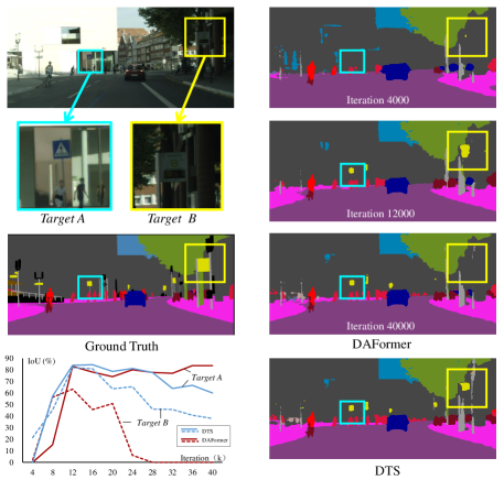
Figure 1: Segmentation results on a test image from Cityscapes (the model is trained on GTAv). There are two traffic signs with different styles, where Target A is similar to the training data in the source domain while Target B is not. The baseline (DAFormer) gradually improves the accuracy on Target A but achieves the best accuracy on Target B in the midst (at $12\mathrm{K}$ iterations). Our method, DTS, achieves good accuracy for both targets and the trend is more stable throughout the training process (see the curves).

The state-of-the-art UDA approaches for semantic segmentation are mostly built upon a self-training framework. It first learns semantics from labeled data in the source domain and then generates pseudo labels in the target domain, so that the model adapts to the target domain by fitting the pseudo labels. Conceptually, the two steps of self-training endow the model with two-fold abilities, namely, learning knowledge (semantics) from the source domain and adapting the knowledge to the target domain.

However, these two abilities can conflict with each other. Figure 1 shows an example of two targets of the same class (traffic sign), where Target A is close to the typical training samples in the source domain, while Target B has a quite different appearance. Using the default setting of DAFormer [19] (a UDA baseline), the recognition accuracy of Target A gradually increases while that of Target B grows first but eventually drops to 0. Interestingly, if one increases the proportion of training samples from the target domain, the recognition quality of Target B will be better while the recognition accuracy of some unexpected classes (e.g., sidewalk) may drop significantly (see details in Appendix A). The conflict sets an obstacle to achieving higher UDA accuracy.

The above analysis prompts us to design a dual teacher-student (DTS) framework. The key is to train two individual models (with different network weights) so that the aforementioned conflict is alleviated. DTS can be built upon most existing self-training approaches in three steps: (1) making two copies of the original teacher-student model, (2) increasing the proportion of training data from the target domain in the second group, and (3) applying a bidirectional learning strategy so that two models supervise each other via pseudo labels. DTS allows the system to pursue a stronger adapting ability (with the second model) meanwhile the learning ability (guaranteed by the first model) is mostly unaffected.

We conduct semantic segmentation experiments with the standard UDA setting. Two synthetic datasets with dense labels, GTAv [37] and SYNTHIA [38], are used as the source domains, and a real dataset with only images, Cityscapes [5], is used as the target domain. We establish the DTS framework upon three recent self-training baselines, namely, DAFormer [19], HRDA [20], and MIC [21]. DTS improves the segmentation accuracy in every single trial, demonstrating its generalized ability across baselines and datasets. In particular, when integrated with MIC, the prior state-of-the-art, DTS reports $76.5\%$ and $67.8\%$ mIoUs on GTAv$\rightarrow$Cityscapes and SYNTHIA$\rightarrow$Cityscapes, respectively, setting new records for both benchmarks.

2 Related Work

Unsupervised domain adaptation (UDA), the task of transferring semantics from labeled source domains to unlabeled target domains, has been widely studied for many computer vision fields, e.g., classification [32, 51, 47], object detection [15, 24, 41], face recognition [25, 18, 40], semantic segmentation [17, 53], etc.

We briefly review two representative UDA approaches for semantic segmentation. Adversarial learning [43, 45] reduces the gap between the source and target domains by confusing a discriminator trained to judge which domain the extracted visual features come from. It is closely related to style transfer methods [16, 49, 11, 50] that synthesize data to simulate the target domain. Self-training instead generates pseudo labels for the unlabeled target images and fits the model accordingly. There is a specific class of self-training methods [44, 9, 55] which further bridge the domain gap by creating mixed images that cover both domains [36], inheriting benefits from style transferring. Many follow-up works [19, 20, 21], including this paper, were based on the self-training framework. Besides UDA, other data-efficient learning scenarios such as semi-supervised [22, 39] and few-shot [31, 35] learning also made use of self-training. Generating high-quality pseudo labels is crucial for self-training. Researchers developed various strategies, such as entropy minimization [3], class-balanced training [30], consistency regularization [21], auxiliary task learning [23, 48], etc., for this purpose.

A fundamental concept in self-training is teacher-student optimization, a concept closely related to knowledge distillation [14, 12, 34]. The methodology was first applied to train a (smaller) student model which acquires stronger abilities by mimicking a (larger) teacher model. To boost the effect of teacher-student optimization, efforts were made in generating high-quality pseudo labels with stronger teacher models [42, 27, 29, 10] and/or preventing error transmission from the teacher model to the student model [26, 56, 22, 4]. There are also other improvements including using multiple student models [54], designing a better loss function [10], etc.

3 Our Approach

We investigate the task of unsupervised domain adaptation (UDA) for semantic segmentation, where a labeled source domain $\mathbb{S}$ and an unlabeled target domain $\mathbb{T}$ are available. We denote the source dataset as $\mathcal{D}^{\mathbb{S}}=\{(\mathbf{x}_{n}^{\mathbb{S}},\mathbf{y}_{n}^{\mathbb{S}})\}_{n=1}^{N_{\mathbb{S}}}$, where $\mathbf{x}_{n}^{\mathbb{S}}$ is an image and $\mathbf{y}_{n}^{\mathbb{S}}$ is the corresponding dense label map. The target dataset $\mathcal{D}^{\mathbb{T}}$ is another set of images without labels, denoted as $\{(\mathbf{x}_{n}^{\mathbb{T}})\}_{n=1}^{N_{\mathbb{T}}}$. The two domains share the same set of categories. The goal of UDA is to train a segmentation network $f(\mathbf{x};\boldsymbol{\theta})$ that eventually works well in the target domain.

We first introduce a self-training baseline where a single teacher-student framework is established (Section 3.1). Then, we reveal a conflict when the model is facilitated to focus on the target domain (Section 3.2), which drives us to propose a dual teacher-student framework towards better UDA performance (Section 3.3).

3.1 Single Teacher-Student Baseline

We start with a standard self-training (i.e., teacher-student) baseline which trains a teacher model and a student model denoted as $f^{\mathrm{te}}(\mathbf{x};\boldsymbol{\theta}^{\mathrm{te}})$ and $f^{\mathrm{st}}(\mathbf{x};\boldsymbol{\theta}^{\mathrm{st}})$, respectively. The teacher model is updated using the exponential moving average (EMA) strategy [42]:

$$\boldsymbol{\theta}^{\mathrm{te}}\leftarrow\boldsymbol{\theta}^{\mathrm{te}}\times\lambda+\boldsymbol{\theta}^{\mathrm{st}}\times(1-\lambda),$$ (1)

where $\lambda$ is a constant coefficient which is often close to $1$. The student model is trained for segmentation in both the source and target domains. For the source images, semantic labels are available for supervised learning:

$$\mathcal{L}^{\mathbb{S}}=\mathcal{L}_{\mathrm{CE}}(f^{\mathrm{st}}(\mathbf{x}^{\mathbb{S}}),\mathbf{y}^{\mathbb{S}}),$$ (2)

where $\mathcal{L}_{\mathrm{CE}}$ denotes the pixel-wise cross-entropy loss. For the target images, the teacher model is used to generate a pseudo label $\tilde{\mathbf{y}}^{\mathbb{T}}$ for $\mathbf{x}^{\mathbb{T}}$, and the pixel-wise loss function is computed in a similar way:

$$\mathcal{L}^{\mathbb{T}}=\mathcal{L}_{\mathrm{CE}}(f^{\mathrm{st}}(\mathbf{x}^{\mathbb{T}}),\tilde{\mathbf{y}}^{\mathbb{T}}).$$ (3)

The overall loss is written as $\mathcal{L}=\mathcal{L}^{\mathbb{S}}+\mathcal{L}^{\mathbb{T}}$. In practice, a balancing mechanism is applied [44, 19]: all pixel-wise loss terms computed on the target domain is multiplied by a factor of $\gamma$, which is the proportion of the pseudo-label confidence surpassing a given threshold, $\tau$.

Recently, a series of methods [44, 19, 20, 21] validated that introducing a mixed domain between the source and target domains is helpful for domain adaptation. A typical operation is named ClassMix [36] which samples mixed images by computing

$$\mathbf{x}_{i,j}^{\langle\mathbb{S},\mathbb{T}\rangle}=\mathcal{M}(\mathbf{x}_{i}^{\mathbb{S}},\mathbf{x}_{j}^{\mathbb{T}})=\mathbf{x}_{i}^{\mathbb{S}}\odot\mathbf{M}_{i}^{\mathbb{S}}+\mathbf{x}_{j}^{\mathbb{T}}\odot(\mathbf{1}-\mathbf{M}_{i}^{\mathbb{S}}),$$ (4)

where $\langle\mathbb{S,T}\rangle$ denotes a mixed domain, $\odot$ is element-wise multiplication, and $\mathbf{M}^{\mathbb{S}}$ is a mask generated by randomly a few class-level masks from the $\mathbf{y}^{\mathbb{S}}$. Accordingly, the target domain in Eqn (3) and the overall loss is replaced with the mixed domain. Note that pseudo labels are only computed for the target portion of the mixed images – we refer the reader to [36] for technical details.

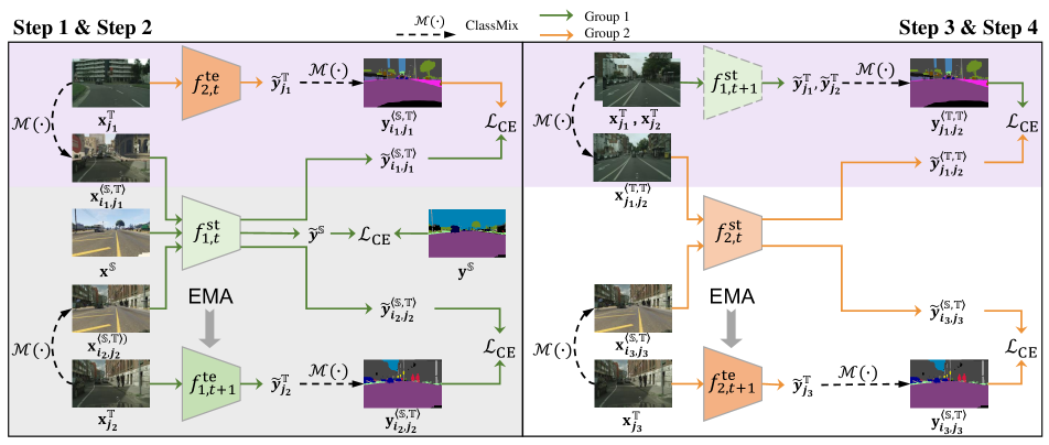
Figure 2: An illustration of the proposed DTS framework, where we use Setting B as an example. The left and right parts describe the optimization of the first and second group models, respectively. The bottom-left part (in gray) corresponds to a single teacher-student framework where ClassMix is used for domain mixing, and the top part (in purple) shows the bidirectional learning strategy, i.e., models from the other group are used for pseudo label generation.

3.2 Conflict between Learning and Adapting

Although domain mixing improves the accuracy of UDA segmentation on several benchmarks, we observe that the trained model is easily biased towards the source domain and thus ignores the target domain to some extent. A typical example is shown in Figure 1.

We conjecture that it is the ‘over-focus’ on the source domain that prevents the model from achieving higher segmentation accuracy. To reveal this, we revisit the working mechanism of ClassMix. Compared to the original strategy that directly generates pseudo labels on the target images, ClassMix increases the proportion of data from the source domain (in a default setting of Eqn (4), an average of half target-domain pixels are replaced with source-domain pixels). This brings two differences. On the one hand, the quality of pseudo labels is improved because part of them are inherited from the labels in the source domain; on the other hand, the focus on the target domain is weakened, increasing the risk of domain adaptation.

Label	$\langle\mathbb{S},\mathbb{T}\rangle$	$\langle\mathbb{T},\mathbb{T}\rangle$	Supervised
w/ pseudo labels	68.3	67.2	–
(pseudo acc.)	64.9	64.2	–
w/ ground-truth	74.4	76.9	77.8

Table 1: UDA segmentation mIoU (%) using DAFormer [19] on the GTAv$\rightarrow$Cityscapes benchmark with different options. An italic number indicates a result that uses target-domain labels. The pseudo accuracy is computed on the training set of Cityscapes.

The above analysis prompts us to perform the ‘Focus on Your Target’ trail towards higher UDA accuracy. We replace the mixed domain of ClassMix, $\langle\mathbb{S},\mathbb{T}\rangle$, with another domain, $\langle\mathbb{T},\mathbb{T}\rangle$, in which the mixed samples are generated using two target images:

$$\mathbf{x}_{j_{1},j_{2}}^{\langle\mathbb{T},\mathbb{T}\rangle}=\mathcal{M}(\mathbf{x}_{j_{1}}^{\mathbb{T}},\mathbf{x}_{j_{2}}^{\mathbb{T}})=\mathbf{x}_{j_{1}}^{\mathbb{T}}\odot\mathbf{M}_{j_{1}}^{\mathbb{T}}+\mathbf{x}_{j_{2}}^{\mathbb{T}}\odot(\mathbf{1}-\mathbf{M}_{j_{1}}^{\mathbb{T}}),$$ (5)

and the pseudo label is adjusted accordingly.

In Table 1, we run DAFormer [19] with either $\langle\mathbb{S},\mathbb{T}\rangle$ or $\langle\mathbb{T},\mathbb{T}\rangle$ for UDA segmentation on GTAv$\rightarrow$Cityscapes. Compared to $\langle\mathbb{S},\mathbb{T}\rangle$, $\langle\mathbb{T},\mathbb{T}\rangle$ achieves an inferior mIoU of $67.2\%$ (a $1.3\%$ drop). But, interestingly, when ground-truth labels are used for the mixed images, the mIoU surpasses the original option by $2.5\%$, with merely a $0.9\%$ mIoU lower than the supervised baseline. In other words, ‘Focus on Your Target’ improves the upper bound, but the models cannot achieve the upper bound because the pseudo labels deteriorate: it is a side effect of decreasing the proportion of training data from the source domain.

In summary, a strong algorithm for UDA shall be equipped with two critical abilities: (i) learning reliable semantics from the source domain, and (ii) adapting the learned semantics to the target domain. However, in the above self-training framework where a single teacher-student model is used, there seems a conflict between these two abilities, e.g., increasing the proportion of target-domain data strengthens the ‘adapting ability’ but weakens the ‘learning ability’, setting an obstacle to better performance. In what follows, we offer a solution by training two teacher-student models simultaneously.

3.3 Dual Teacher-Student Framework

The proposed dual teacher-student (DTS) framework is illustrated in Figure 2. We denote the models used in the two teacher-student groups as $f_{1}^{\mathrm{te}}(\mathbf{x};\boldsymbol{\theta}_{1}^{\mathrm{te}})$, $f_{1}^{\mathrm{st}}(\mathbf{x};\boldsymbol{\theta}_{1}^{\mathrm{st}})$ and $f_{2}^{\mathrm{te}}(\mathbf{x};\boldsymbol{\theta}_{2}^{\mathrm{te}})$, $f_{2}^{\mathrm{st}}(\mathbf{x};\boldsymbol{\theta}_{2}^{\mathrm{st}})$, respectively, where we use a subscript (1 or 2) to indicate the group ID. As described above, we expect the first teacher-student model to stick to learning reliable semantics from the source domain, while the second teacher-student model learns to ‘Focus on Your Target’ to enhance the adapting ability.

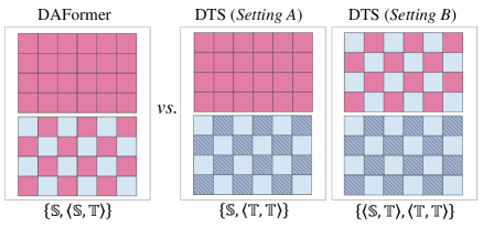
Figure 3: An illustration of different combinations of training data. We use magenta to represent source-domain patches and two types of blue to represent target-domain patches from different images. In practice, the images are not partitioned into regular grids, but into semantic regions according to the (real or pseudo) labels.

We achieve the goal by using different data proportions for the two groups. An illustration is provided in Figure 3. The first group remains the same as in the baseline, i.e., half of the training samples are simply source images and another half are ClassMix-ed images covering the source and target domains. Using the previously defined notations, we denote the combination as $\{\mathbb{S},\langle\mathbb{S},\mathbb{T}\rangle\}$. To increase the proportion of the target-domain data, we first change the mixture of data from $\langle\mathbb{S},\mathbb{T}\rangle$ to $\langle\mathbb{T},\mathbb{T}\rangle$ (i.e., same as that used in the ‘Focus on Your Target’ trial), and then replace the pure source domain with $\langle\mathbb{S},\mathbb{T}\rangle$. That said, we create two settings for data combination, $\{\mathbb{S},\langle\mathbb{T},\mathbb{T}\rangle\}$ and $\{\langle\mathbb{S},\mathbb{T}\rangle,\langle\mathbb{T},\mathbb{T}\rangle\}$. We name them Setting A and Setting B of the second group throughout the remainder of this paper. Intuitively, the proportion of the target-domain data is increased from around $25\%$ in the first group (as well as the baselines) to around $50\%$/$75\%$ using Setting A/Setting B in the second group.

There are two teacher models and two student models to be optimized. We perform iterative optimization and propose a bidirectional learning strategy so that each teacher-student model propagates information to the other by contributing to the generation of pseudo labels. In the $t$-th iteration, we perform the following steps orderly:
 
(1) Updating $f_{1,t+1}^{\mathrm{te}}(\cdot)$ using the EMA of $f_{1,t}^{\mathrm{st}}(\cdot)$.
(2) Updating $f_{1,t+1}^{\mathrm{st}}(\cdot)$. This is done by generating a batch of images in the domain of $\langle\mathbb{S},\mathbb{T}\rangle$, feeding half of them into $f_{1,t+1}^{\mathrm{te}}(\cdot)$ and another half to $f_{2,t}^{\mathrm{te}}(\cdot)$ for generating pseudo labels. $f_{1,t+1}^{\mathrm{st}}(\cdot)$ is updated with gradient back-propagation using the pseudo labels and the true labels in $\mathbb{S}$.
(3) Updating $f_{2,t+1}^{\mathrm{te}}(\cdot)$ using the EMA of $f_{2,t}^{\mathrm{st}}(\cdot)$.
(4) Updating $f_{2,t+1}^{\mathrm{st}}(\cdot)$. This is done by generating a batch of images in the domain of $\langle\mathbb{T},\mathbb{T}\rangle$ (and also $\langle\mathbb{S},\mathbb{T}\rangle$ if Setting B is used), feeding half of them into $f_{2,t+1}^{\mathrm{te}}(\cdot)$ and another half to $f_{1,t+1}^{\mathrm{st}}(\cdot)$ for generating pseudo labels. $f_{2,t+1}^{\mathrm{st}}(\cdot)$ is updated with gradient back-propagation using the pseudo labels and the true labels in $\mathbb{S}$. The idea of using $f_{1,t+1}^{\mathrm{st}}(\cdot)$ (a model from the next iteration) for generating pseudo labels is known as ‘learning from future’ [7] which improves the quality of pseudo labels for the current iteration.
  Finally, after a total of $T$ training iterations, $f_{2,T}^{\mathrm{st}}(\cdot)$ is chosen as the final model for inference.

Note that, if $f_{2,t}^{\mathrm{te}}(\cdot)$ is not used in Step 2 (i.e., all pseudo labels are generated using $f_{1,t+1}^{\mathrm{te}}(\cdot)$), the information is only propagated from the first teacher-student model to the second one, hence the optimization strategy is degenerated from bidirectional to unidirectional. The advantage of the bidirectional strategy, as well as other design choices, will be diagnosed in the experimental section.

Method	Road	Sidewalk	Building	Wall	Fence	Pole	Light	Sign	Veg	Terrain	Sky	Person	Rider	Car	Truck	Bus	Train	Motor	Bike	mIoU
AdaptSegNet [45]	86.5	36.0	79.9	23.4	23.3	23.9	35.2	14.8	83.4	33.3	75.6	58.5	27.6	73.7	32.5	35.4	3.9	30.1	28.1	42.4
PatchAligne [46]	92.3	51.9	82.1	29.2	25.1	24.5	33.8	33.0	82.4	32.8	82.2	58.6	27.2	84.3	33.4	46.3	2.2	29.5	32.3	46.5
FDA [50]	92.5	53.3	82.4	26.5	27.6	36.4	40.6	38.9	82.3	39.8	78.0	62.6	34.4	84.9	34.1	53.1	16.9	27.7	46.4	50.5
DACS [44]	89.9	39.7	87.9	39.7	39.5	38.5	46.4	52.8	88.0	44.0	88.8	67.2	35.8	84.5	45.7	50.2	0.0	27.3	34.0	52.1
ProDA [52]	87.8	56.0	79.7	46.3	44.8	45.6	53.5	53.5	88.6	45.2	82.1	70.7	39.2	88.8	45.5	50.4	1.0	48.9	56.4	57.5
DAP [23]	94.5	63.1	89.1	29.8	47.5	50.4	56.7	58.7	89.5	50.2	87.0	73.6	38.6	91.3	50.2	52.9	0.0	50.2	63.5	59.8
CPSL [30]	92.3	59.9	84.9	45.7	29.7	52.8	61.5	59.5	87.9	41.6	85.0	73.0	35.5	90.4	48.7	73.9	26.3	53.8	53.9	60.8
DAFormer [19]	95.7	70.2	89.4	53.5	48.1	49.6	55.8	59.4	89.9	47.9	92.5	72.2	44.7	92.3	74.5	78.2	65.1	55.9	61.8	68.3
DAFormer+FST [7]	95.3	67.7	89.3	55.5	47.1	50.1	57.2	58.6	89.9	51.0	92.9	72.7	46.3	92.5	78.0	81.6	74.4	57.7	62.6	69.3
DAFormer+CAMix [55]	96.0	73.1	89.5	53.9	50.8	51.7	58.7	64.9	90.0	51.2	92.2	71.8	44.0	92.8	78.7	82.3	70.9	54.1	64.3	70.0
DAFormer+DTS (ours)	96.8	76.0	90.0	56.5	50.1	51.9	57.4	65.1	90.5	50.5	92.4	73.5	46.9	93.0	80.4	85.2	74.0	58.7	63.5	71.2
HRDA [20]	96.4	74.4	91.0	61.6	51.5	57.1	63.9	69.3	91.3	48.4	94.2	79.0	52.9	93.9	84.1	85.7	75.9	63.9	67.5	73.8
HRDA+DTS (ours)	96.7	76.3	91.3	60.7	55.9	59.9	67.3	72.5	91.8	50.1	94.4	80.7	56.8	94.4	86.0	86.0	73.9	65.7	68.4	75.2
MIC [21]	97.4	80.1	91.7	61.2	56.9	59.7	66.0	71.3	91.7	51.4	94.3	79.8	56.1	94.6	85.4	90.3	80.4	64.5	68.5	75.9
MIC+DTS (ours)	97.0	80.4	91.8	60.6	58.7	61.7	67.9	73.2	92.0	45.4	94.3	81.3	58.7	95.0	87.9	90.7	82.2	65.7	69.0	76.5

Table 2: UDA segmentation accuracy (mIoU, %) on the GTAv$\rightarrow$Cityscapes benchmark. The highest number in each column is marked with bold. The results in the first group are obtained on a ResNet101 backbone and the others are obtained on a MiT-B5 backbone.

3.4 Technical Details

Choosing the proper option for data combination. We compute the averaged confidence of pseudo labels generated by the corresponding teacher models, $f_{1}^{\mathrm{st}}(\cdot)$ and $f_{2}^{\mathrm{te}}(\cdot)$. Following [44, 19], $\gamma$ is defined as the proportion of pixels with the max class score surpassing a given threshold, $\tau$. For each training image $\mathbf{x}$, we use $\gamma_{1}^{\mathrm{st}}(\mathbf{x})$ and $\gamma_{2}^{\mathrm{te}}(\mathbf{x})$ to denote the average $\gamma$ values over all pixels when the teacher models are $f_{1}^{\mathrm{st}}(\cdot)$ and $f_{2}^{\mathrm{te}}(\cdot)$, respectively. Then, we estimate the chance that $f_{2}^{\mathrm{te}}(\cdot)$ generates better pseudo labels than $f_{1}^{\mathrm{st}}(\cdot)$:

$$\mathrm{Prob}=\mathbb{E}_{\mathbf{x}\sim\mathcal{D}^{\mathbb{T}}}\left[\mathbb{I}({\gamma}_{2}^{\mathrm{te}}(\mathbf{x})>{\gamma}_{1}^{\mathrm{st}}(\mathbf{x}))\right],$$ (6)

where $\mathbb{I}(\cdot)$ is the indicator function that outputs $1$ if the statement is true and $0$ otherwise. Note that the estimation is performed individually for two training procedures using Setting A and Setting B. Finally, we choose the setting with a higher chance that $f_{2}^{\mathrm{te}}(\cdot)$ is more confident because $f_{2}^{\mathrm{st}}(\cdot)$ is eventually used for inference. We shall see in Section 4.3 that this criterion always leads to the better choice.

Generating the mask. In the domain mixing operation, we compute the mask $\mathbf{M}$ by choosing the class label of one image. If the $\langle\mathbb{S},\mathbb{T}\rangle$ is used, the source image with ground-truth is chosen; if $\langle\mathbb{T},\mathbb{T}\rangle$ is used, the image with a larger average value of $\gamma$ is chosen.

Generating pseudo labels. The details are slightly different between Setting A and Setting B. When the batch size is $k$, the number of target images used for the second group in Setting A and Setting B are $2k$ and $3k$, respectively. For Setting A, $k$ pseudo labels used are generated by $f_{1,t+1}^{\mathrm{st}}(\cdot)$ and other $k$ by $f_{2,t+1}^{\mathrm{te}}(\cdot)$. For Setting B, the $2k$ pseudo labels used in $\langle\mathbb{T},\mathbb{T}\rangle$ are generated by $f_{1,t+1}^{\mathrm{st}}(\cdot)$ and the $k$ labels used in $\langle\mathbb{S},\mathbb{T}\rangle$ are generated by $f_{2,t+1}^{\mathrm{te}}(\cdot)$.

4 Experiments

4.1 Datasets and Settings

Datasets. We train the models on a labeled source domain and an unlabeled target domain and test them on the target domain. We follow the convention to set the source domain to be a synthesized dataset (either GTAv [37] which contains $24\rm{,}966$ densely labeled training images at a resolution of $1914\times 1052$ or SYNTHIA [38] which contains $9\rm{,}400$ densely labeled training images at a resolution of $1280\times 760$), and the target dataset to be a real dataset (Cityscapes [5] where only the finely-annotated subset is used, containing $2\rm{,}975$ training images and $500$ validation images at a resolution of $2048\times 1024$). Following the convention to report the mean IoU (mIoU) over $19$ classes when GTAv is used as the source domain, and $13$ or $16$ classes when SYNTHIA is the source domain.

Training details. Our framework is applied to different self-training frameworks. Specifically, we follow the DAFormer series [19, 20, 21] where the encoder is a MiT-B5 model pre-trained on ImageNet-1K [6] and the decoder involves a context-aware feature fusion module. We train the framework on a single NVIDIA Tesla-V100 GPU for $40\mathrm{K}$ iterations with a batch size of $2$ for both groups. We use an AdamW optimizer [33] with learning rates of $6\times 10^{-5}$ for the encoder and $6\times 10^{-4}$ for the decoder, a weight decay of $0.01$, and linear warm-up of the learning rate for the first $1.5\mathrm{K}$ iterations. The input image size is always $512\times 512$. During the training phase, we apply random rescaling and cropping to the source and target data, as well as color jittering and Gaussian blur as strong augmentations for the mixed data. The EMA coefficient, $\lambda$, is set to be $0.999$. The pseudo-label confidence threshold, $\tau$, is $0.968$ as in [44].

Method	Road	Sidewalk	Building	Wall*	Fence*	Pole*	Light	Sign	Veg	Sky	Person	Rider	Car	Bus	Motor	Bike	mIoU	mIoU*
PatchAlign [46]	82.4	38.0	78.6	8.7	0.6	26.0	3.9	11.1	75.5	84.6	53.5	21.6	71.4	32.6	19.3	31.7	40.0	46.5
AdaptSegNet [45]	84.3	42.7	77.5	–	–	–	4.7	7.0	77.9	82.5	54.3	21.0	72.3	32.2	18.9	32.3	–	46.7
FDA [50]	79.3	35.0	73.2	–	–	–	19.9	24.0	61.7	82.6	61.4	31.1	83.9	40.8	38.4	51.1	–	52.5
DACS [44]	80.6	25.1	81.9	21.5	2.9	37.2	22.7	24.0	83.7	90.8	67.6	38.3	82.9	38.9	28.5	47.6	48.3	54.8
ProDA [52]	87.8	45.7	84.6	37.1	0.6	44.0	54.6	37.0	88.1	84.4	74.2	24.3	88.2	51.1	40.5	45.6	55.5	62.0
DAP [23]	84.2	46.5	82.5	35.1	0.2	46.7	53.6	45.7	89.3	87.5	75.7	34.6	91.7	73.5	49.4	60.5	59.8	64.3
CPSL [30]	87.2	43.9	85.5	33.6	0.3	47.7	57.4	37.2	87.8	88.5	79.0	32.0	90.6	49.4	50.8	59.8	57.9	65.3
DAFormer [19]	84.5	40.7	88.4	41.5	6.5	50.0	55.0	54.6	86.0	89.8	73.2	48.2	87.2	53.2	53.9	61.7	60.9	67.4
DAFormer+FST [7]	88.3	46.1	88.0	41.7	7.3	50.1	53.6	52.5	87.4	91.5	73.9	48.1	85.3	58.6	55.9	63.4	61.9	68.7
DAFormer+CAMix [55]	87.4	47.5	88.8	–	–	–	55.2	55.4	87.0	91.7	72.0	49.3	86.9	57.0	57.5	63.6	–	69.2
DAFormer+DTS (ours)	88.5	51.4	88.0	37.2	4.8	51.4	59.4	59.0	88.1	92.7	71.3	51.3	89.2	67.7	58.4	62.8	63.8	71.4
HRDA [20]	85.2	47.7	88.8	49.5	4.8	57.2	65.7	60.9	85.3	92.9	79.4	52.8	89.0	64.7	63.9	64.9	65.8	72.4
HRDA+DTS (ours)	88.5	53.1	88.7	44.0	5.8	59.2	68.3	60.7	87.7	93.4	79.5	46.4	91.3	64.2	66.8	65.9	66.5	73.4
MIC [21]	86.6	50.5	89.3	47.9	7.8	59.4	66.7	63.4	87.1	94.6	81.0	58.9	90.1	61.9	67.1	64.3	67.3	74.0
MIC+DTS (ours)	89.1	54.9	89.0	39.1	8.7	61.6	67.4	64.3	88.8	94.0	82.2	60.7	89.6	62.6	68.5	64.9	67.8	75.1

Table 3: UDA segmentation accuracy (mIoU, %) on the SYNTHIA$\rightarrow$Cityscapes benchmark. The highest number in each column is marked with bold. The results in the first group are obtained on a ResNet101 backbone and the others are obtained on a MiT-B5 backbone. The mIoU and mIoU* columns denote the averaged IoU over $16$ and $13$ classes, where the latter does not contain the classes marked with *.

4.2 Comparison to the State-of-the-art Methods

We compare DTS to state-of-the-art UDA approaches on the GTAv$\rightarrow$Cityscapes and SYNTHIA$\rightarrow$Cityscapes benchmarks. Results are summarized in Table 2 and Table 3, respectively. We establish DTS upon three recently published works, namely, DAFormer [19], HRDA [20], and MIC [21].

DTS reports consistent gains in terms of segmentation accuracy beyond all three baselines. On GTAv$\rightarrow$Cityscapes and SYNTHIA$\rightarrow$Cityscapes ($13$ classes), the mIoU gains over DAFormer, HRDA, MIC are $2.9\%$, $1.4\%$, $0.6\%$ and $4.0\%$, $1.0\%$, $1.1\%$ respectively. The gain generally becomes smaller when the baseline is stronger, which is as expected. Specifically, when added to MIC, the previous best approach, DTS achieves new records on these benchmarks: a $76.5\%$ mIoU on GTAv$\rightarrow$Cityscapes and $67.8\%$ and $75.1\%$ mIoUs on SYNTHIA$\rightarrow$Cityscapes with $16$ and $13$ classes, respectively.

Comparison to FST. We compare DTS to another plug-in approach, FST [7]. On DAFormer, the gains brought by FST on the two benchmarks (SYNTHIA using $13$ classes) are $1.0\%$ and $1.3\%$, while the numbers for DTS are $2.9\%$ and $4.0\%$, respectively. That said, besides the contribution of FST that allows us to ‘learn from future’, the higher accuracy also owes to the design of the DTS framework that alleviates the conflict of learning and adapting.

Class-level analysis. We investigate which classes are best improved by DTS. On GTAv$\rightarrow$Cityscapes, we detect two classes, sign and truck, on which the IoU gain on the three baselines is always higher than the mIoU gain. In Appendix B, we show that these classes suffer larger variations between the source-domain and target-domain appearances, and hence the learned features are more difficult to transfer. They are largely benefited by the ‘Focus on Your Target’ ability of DTS.

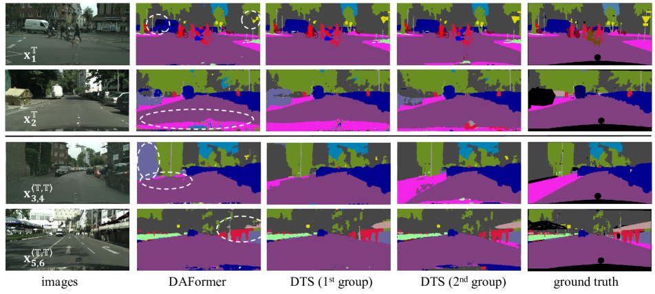
Figure 4: Visualization of the segmentation results of DAFormer [19] and DTS. The top two rows display two real images and the bottom two rows display two synthesized images from $\langle\mathbb{T},\mathbb{T}\rangle$. In each group, the first example is from GTAv$\rightarrow$Cityscapes and the second one is from SYNTHIA$\rightarrow$Cityscapes. The white, dashed circles highlight the regions that are significantly improved by DTS.

Visualization. We visualize the segmentation results of DAFormer and DAFormer+DTS in Figure 4. For the real images, the advantage of DTS is significant on the classes that are easily confused with others (e.g., sidewalk which is visually similar to road) or suffer large domain shifts (e.g., sign or truck). For the mixed images, we find that the baseline model is easily confused by the unusual stitching and/or discontinuous textures because it has never seen such patterns in the source domain – in such cases, the model of the second group is generally better and sometimes it can propagate the advantages to the model of the first group, revealing the advantage of bidirectional learning.

4.3 Diagnostic Studies

Setting	Choice and Accuracy
Dual Teacher-Student			✓	✓	✓
‘Focus on Your Target’		✓	✓		✓
Bidirectional Learning				✓	✓
GTA$\rightarrow$Cityscapes	68.3	67.2	69.7	68.6	71.2
SYNTHIA$\rightarrow$Cityscapes	60.9	58.4	63.3	61.2	63.7

Table 4: Ablative studies of DTS with respect to the UDA segmentation accuracy (mIoU, %) on both benchmarks. All these experiments are based on DAFormer [19]. For SYNTHIA$\rightarrow$Cityscapes, the mIoUs are computed over $16$ classes.

Ablative studies. We first diagnose the proposed approach by ablating the contribution of three components, namely, applying the dual teacher-student (DTS) framework, increasing the proportion of data from the target domain (i.e., ‘Focus on Your Target’), and adopting the bidirectional learning strategy. Results are summarized in Table 4. Note that some combinations are not valid, e.g., solely applying DTS (without adjusting the proportion of training data nor applying bidirectional learning) does not make any difference from the baseline; also, bidirectional learning must be built upon DTS.

From Columns 1–3, one can learn the importance of the DTS framework. When DTS is not established, simply increasing the proportion of target data (Col 2) incurs an accuracy drop on both GTA$\rightarrow$Cityscapes and SYNTHIA$\rightarrow$Cityscapes. This validates our motivation, i.e., there is a conflict between the learning and adapting abilities. However, after the dual teacher-student framework is established (Col 3, where the first teacher-student group focuses on learning and the second group focuses on adapting), the conflict is weakened and the accuracy gain becomes clear ($1.6\%$ on GTA$\rightarrow$Cityscapes and $2.4\%$ on SYNTHIA$\rightarrow$Cityscapes).

From Columns 3–5, one can observe the contribution of ‘Focus on Your Target’ (i.e., increasing the proportion of target data) and bidirectional learning on top of the DTS framework. The best practice is obtained when all the modules are used (Col 5), aligning with the results reported in Tables 2 and 3. Interestingly, when bidirectional learning is adopted alone (Col 4), the accuracy gain is much smaller than that of using ‘Focus on Your Target’ alone, because the two groups are using the same proportion of data mixing, and thus the bidirectional learning carries limited complementary information.

Baseline		DAFormer	HRDA	MIC
GTAv	Setting A	70.3	74.7	76.5
	Setting B	71.2	75.2	76.2
SYNTHIA	Setting A	63.8	66.5	67.8
	Setting B	61.2	66.0	67.2

Table 5: The results of DTS with different data mixing options. For SYNTHIA$\rightarrow$Cityscapes, the mIoUs are computed over $16$ classes.

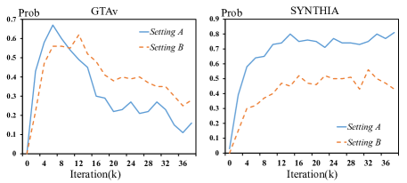
Figure 5: The curves of $\mathrm{Prob}$ computed on the GTAv$\rightarrow$Cityscapes and SYNTHIA$\rightarrow$Cityscapes benchmarks. DAFormer is used as the baseline. These curves suggest that, on DAFormer, Setting B is better for GTAv$\rightarrow$Cityscapes while Setting A is better for SYNTHIA$\rightarrow$Cityscapes.

Choose the option for data combination. We validate that the data combination option can be chosen by comparing the pseudo-label confidence, as described in Section 3.4. We plot the $\mathrm{Prob}$ curves throughout training procedure of Setting A and Setting B in Figure 5. On GTAv$\rightarrow$Cityscapes, the $\mathrm{Prob}$ value of Setting B is eventually higher than that of Setting A, and DTS with Setting B outperforms DTS with Setting A by a $0.9\%$ mIoU (see Table 5). However, on SYNTHIA$\rightarrow$Cityscapes, the $\mathrm{Prob}$ value of Setting A is always higher than that of Setting B, and DTS with Setting A outperforms DTS with Setting B by a $2.4\%$ mIoU. Table 5 also shows the segmentation accuracy on the other two baselines. All choices of advantageous results align with the aforementioned criterion.

Group #1		Group #2		mIoU
$f_{2,t}^{\mathrm{st}}(\cdot)$	$f_{2,t}^{\mathrm{te}}(\cdot)$	$f_{1,t+1}^{\mathrm{st}}(\cdot)$	$f_{1,t+1}^{\mathrm{te}}(\cdot)$
	✓		✓	68.5†
✓			✓	69.0
	✓		✓	69.5
✓		✓		70.2
	✓	✓		71.3

Table 6: UDA segmentation accuracy (mIoU, %) using different models to generate pseudo labels on GTAv$\rightarrow$Citysacpes. ^†: In the first row, each group only uses the teacher model from the other group; in other cases, each group also uses its own teacher models (not presented in the table).

Models for pseudo label generation. We study the impact of different models for generating pseudo labels. Results are summarized in Table 6. When each teacher-student group only uses the teacher model from another group (the first row), there is almost no accuracy gain (the baseline is $68.3\%$), indicating the necessity of the supervision signals from its own teacher.

Then, we discuss the situations where each group uses its teacher and one model from the other group. For the second teacher-student group, using $f_{1,t+1}^{\mathrm{st}}(\cdot)$ as the teacher is superior to using $f_{1,t+1}^{\mathrm{te}}(\cdot)$, because the former model is optimized one more iteration and thus produces better semantics (i.e., ‘learning from future’). For the first teacher-student group, only models from the current iteration of the second group can be used, and $f_{2,t}^{\mathrm{te}}(\cdot)$ always works better than $f_{2,t}^{\mathrm{st}}(\cdot)$, implying the advantage of EMA.

Method	GTAv$\rightarrow$City.		SYNTHIA$\rightarrow$City.
	DACS	DAFormer	DACS	DAFormer
w/o DTS	53.9	56.0	54.2	53.5
w DTS	55.2	59.9	56.6	56.9

Table 7: UDA segmentation accuracy (mIoU, %) on two CNN-based backbones and two benchmarks.

DTS applied to other backbones. To show that DTS adapts to different network backbones (e.g., CNNs), we follow the previous approaches [50, 44, 23] to inherit a ResNet101 [13] pre-trained on ImageNet and MSCOCO and train it using DeepLabV2 [1]. The other settings remain unchanged. Results are listed in Table 7. Still, DTS brings consistent accuracy gains, improving DACS and DAfromer by $1.3\%$ and $3.9\%$ on GTAv$\rightarrow$Cityscapes, and by $2.4\%$ and $3.4\%$ on SYNTHIA$\rightarrow$Cityscapes. Class-wise comparison can refer to Appendix C. These experiments validate that DTS is a generalized UDA framework that does not rely on specific network architectures.

Application to semi-supervised semantic segmentation. As a generalized self-training framework, DTS can also be applied to semi-supervised segmentation. We conduct experiments on PASCAL VOC [8] and follow the conventional settings to train a DeepLabV3+ model with ResNet101 as the backbone. Other settings remain unchanged; please refer to Appendix E for details. We report the segmentation results in Table 8. Using $1/16$, $1/8$, $1/4$ labeled data, DTS produces consistent accuracy gains of $3.5\%$, $1.7\%$, $0.8\%$ over the MeanTeacher approach [42], and $1.5\%$, $1.3\%$, $1.0\%$ over the re-implemented FST baseline [7]. This validates that semi-supervised learning also benefits from bidirectional learning which effectively improves the ability to learn from the pseudo labels generated from other groups.

Methods	1/16 (662)	1/8 (1323)	1/4 (2646)
Mean Teacher [42]	71.3	75.4	76.5
FST [7]	73.9	76.1	78.1
FST*	73.3	75.8	76.3
DTS (ours)	74.8	77.1	77.3

Table 8: Semi-supervised segmentation mIoU (%) on PASCAL VOC. *: This is our re-implementation of FST.

5 Conclusions

In this paper, we study the UDA segmentation problem from the perspective of endowing the model with two-fold abilities, i.e., learning from the reliable semantics, and adapting to the target domain. We show that these two abilities can conflict with each other in a single teacher-student model, and hence we propose a dual teacher-student (DTS) framework, where the two models stick to the ‘learning ability’ and ‘adapting ability’, respectively. Specifically, the second model learns to ‘focus on your target’ to improve its accuracy in the target domain. We further design a bidirectional learning strategy to facilitate the two models to communicate via generating pseudo labels. We validate the effectiveness of DTS and set new records on two standard UDA segmentation benchmarks.

As the accuracy on the two benchmarks fast approaches the supervised baseline (e.g., a $77.8\%$ mIoU on Cityscapes), we look forward to building larger and higher-quality synthesized datasets to break through the baseline. This is of value to real-world applications, as synthesized data can be generated at low costs. We expect that the proposed methodology can be applied to other scenarios such as domain generalization, with the second group focusing on a generic, unbiased feature space.

Method	Road	Sidewalk	Building	Wall	Fence	Pole	Light	Sign	Veg	Terrain	Sky	Person	Rider	Car	Truck	Bus	Train	Motor	Bike	mIOU
DACS	95.3	67.9	87.5	33.7	30.5	40.2	50.2	56.4	87.7	45.3	87.0	67.4	29.7	89.5	48.0	50.5	2.2	23.0	32.0	53.9
DACS + DTS	96.1	72.2	88.2	38.1	33.6	41.6	52.1	61.4	88.6	50.0	89.1	68.5	38.0	90.6	59.1	58.0	0.2	8.6	14.5	55.2
DAFormer	94.7	66.3	87.9	40.7	33.9	37.2	50.2	52.9	87.9	46.5	88.2	69.8	44.2	89.1	43.1	55.8	0.7	24.7	50.7	56.0
DAFormer+DTS	96.4	73.9	88.6	40.0	39.8	42.2	52.2	63.5	88.8	49.6	89.3	70.6	45.6	90.8	61.1	57.0	0.4	33.1	55.4	59.9
DACS	81.3	38.9	84.6	15.3	1.7	40.2	45.2	50.3	85.0	–	85.3	70.4	41.9	84.6	–	44.8	–	39.8	57.5	54.2
DACS + DTS	88.7	52.7	85.5	7.2	2.5	40.5	48.9	52.1	86.0	–	87.8	72.5	46.8	83.9	–	43.4	–	46.6	60.9	56.6
DAFormer	66.8	29.3	85.0	19.1	2.3	38.7	45.9	51.6	80.8	–	85.9	70.2	41.9	84.9	–	46.0	–	48.9	58.4	53.5
DAFormer+DTS	88.9	52.5	85.1	7.5	2.4	39.7	49.5	52.7	85.6	–	87.0	72.8	47.0	85.0	–	48.0	–	47.7	58.9	56.9

Table 9: Segmentation accuracy (IOU, %) of baselines [44, 19] and DTS based on ResNet101 backbone. The top part shows the transfer results for GTAv$\rightarrow$Cityscapes and the bottom part shows the results for SYNTHIA$\rightarrow$Cityscapes, where mIoU is computed over 16 classes. All results are averaged over $3$ runs.

Appendix A Examples of the Conflict in Learning

We provide an example of the conflict between the learning and adapting abilities, which we discussed in Section 1 of the main article. This is tested using a single teacher-student framework. We use the same test case as in Figure 1, which has two targets of traffic sign with different appearances. When trained on the original data combination, $\{\mathbb{S},\langle\mathbb{S},\mathbb{T}\rangle\}$, the baseline method (DAFormer [19]) shows that Target B (an object with a larger transfer difficulty) gradually grows but eventually drops to $0$, resulting in an overall mIoU of $50.5\%$. When the proportion of the target domain is increased using the combination of $\{\mathbb{S},\langle\mathbb{T},\mathbb{T}\rangle\}$, the model has a better performance on Target B but reports a lower mIoU of $48.1\%$, as shown in Figure 6. Therefore, improving the adaptability of Target B in this framework can potentially deteriorate the learning of other semantic concepts. However, the proposed DTS performs well on Target B without harming the recognition of other classes, hence improving the overall mIoU to $55.2\%$.

Appendix B Statistical Differences between Domains

To make a clear and distinct comparison between the source and target domains, we compute the occurrence frequency of each class in GTAv and Cityscapes. This is done by simply dividing the number of images including a given category by the total number of images – we believe that better metrics can be defined. The comparison of $19$ classes is presented in Figure 7. We can see that the traffic sign and truck classes exhibit a large difference between the two datasets, which is consistent with the difficulties during transfer (see the analysis in Section 4.2 of the main article). Except for these two representative classes, we also find that the fence, traffic light, rider, and bike classes are statistically improved by DTS on three strong baselines (see Table 2), despite them having substantial differences between GTAv and Cityscapes.

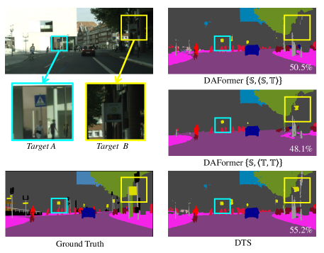
Figure 6: Qualitative and quantitative comparisons of the single teacher-student model trained on different data combination strategies. The numbers shown in the bottom-right corner denote the mIoU of the overall image.

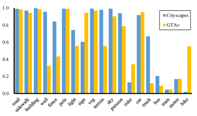
Figure 7: Frequency of subclass occurrence in the source dataset (GTAv) and target dataset (Cityscapes).

Appendix C Results on the CNN-based Backbones

We present the class-wise segmentation accuracy of the CNN-based backbones on both the GTAv$\rightarrow$Cityscapes and SYNTHIA$\rightarrow$Cityscapes benchmarks in Table 9. The proposed DTS approach achieves significant improvements in the traffic sign and truck categories when GTAv is used as the source data, which is consistent with the results obtained using a transformer backbone (see the analysis in the previous section). In the case of using SYNTHIA as the source data, our approach outperforms other methods in the road, sidewalk, person, and rider classes, which are easily confused with each other (road vs. sidewalk, person vs. rider).

Options	GTAv	SYNTHIA
$\{\langle\mathbb{T},\mathbb{T}\rangle\}$	69.1	61.1
$\{\langle\mathbb{S},\mathbb{T}\rangle\}$	69.3	59.4
$\{\mathbb{S},\langle\mathbb{T},\mathbb{T}\rangle\}$	70.3	63.8
$\{\langle\mathbb{S},\mathbb{T}\rangle,\langle\mathbb{T},\mathbb{T}\rangle\}$	71.2	61.2

Table 10: The results of DTS with more data mixing options. We show the mIoU of the $16$ classes in SYNTHIA and make this comparison based on the DAFormer baseline.

Appendix D More Data Combination Options

We propose two data combinations to tune the proportion of target data in our method: $\{\mathbb{S},\langle\mathbb{T},\mathbb{T}\rangle\}$ and $\{\langle\mathbb{S},\mathbb{T}\rangle,\langle\mathbb{T},\mathbb{T}\rangle\}$. While there are two other options to increase the focus on the target domain as well, namely $\{\langle\mathbb{T},\mathbb{T}\rangle\}$ and $\{\langle\mathbb{S},\mathbb{T}\rangle\}$. The two options only include one type of data and have a disadvantage compared to the previous two combinations (see Table 10). $\{\langle\mathbb{T},\mathbb{T}\rangle\}$ means that the second teacher-student group achieves the ability of learning only from the pseudo labels provided by $f_{1}^{\mathrm{st}}(\mathbf{x};\boldsymbol{\theta}_{1}^{\mathrm{st}})$. As a result, noise can easily persist without accurate supervision from the source data. $\{\langle\mathbb{S},\mathbb{T}\rangle\}$ has a similar data proportion as $\{\mathbb{S},\langle\mathbb{T},\mathbb{T}\rangle\}$ but cannot solve the problem of inconsistency between the training and testing data. Using $\langle\mathbb{T},\mathbb{T}\rangle$ as the training domain is an effective way to bridge the gap between the training and testing phases. Therefore, the two combinations containing two different types of data used in DTS are more suitable for balancing the learning and adapting abilities.

Appendix E Details of Semi-supervised Segmentation

Dataset. We perform semi-supervised segmentation on the widely used PASCAL VOC dataset [8], which comprises $20$ object classes and a background class. The training, validation, and testing sets contain $1\rm{,}464$, $1\rm{,}449$, and $1\rm{,}456$ images, respectively. To align with prior works, we use the augmented set, which contains $10\rm{,}582$ images, as the complete training set. During the training, we apply random flipping and cropping to augment the image data and resize the image to $513\times 513$ before feeding it to the models.

Implementation. We perform all experiments using the DeepLabV3+ [2] network with a ResNet-101 backbone pre-trained on ImageNet. An SGD optimizer, with a learning rate of $0.0001$ for the encoder and $0.001$ for the decoder, and a weight decay of $0.0001$, is used. The batch size of both labeled and unlabeled data is $16$ for each group teacher-student. We train the models for $40$ epochs and report the average of three runs for all the results. Since there is no domain gap between the labeled and unlabeled parts, only a dual teacher-student framework and bidirectional learning are applied in the semi-supervised experiments.

References

- [1] Liang-Chieh Chen, George Papandreou, Iasonas Kokkinos, Kevin Murphy, and Alan L Yuille. Deeplab: Semantic image segmentation with deep convolutional nets, atrous convolution, and fully connected crfs. IEEE Transactions on Pattern Analysis and Machine Intelligence, 40(4):834–848, 2017.
- [2] Liang-Chieh Chen, Yukun Zhu, George Papandreou, Florian Schroff, and Hartwig Adam. Encoder-decoder with atrous separable convolution for semantic image segmentation. In Proceedings of the European conference on computer vision (ECCV), pages 801–818, 2018.
- [3] Minghao Chen, Hongyang Xue, and Deng Cai. Domain adaptation for semantic segmentation with maximum squares loss. In Proceedings of the IEEE/CVF International Conference on Computer Vision, pages 2090–2099, 2019.
- [4] Xiaokang Chen, Yuhui Yuan, Gang Zeng, and Jingdong Wang. Semi-supervised semantic segmentation with cross pseudo supervision. In Proceedings of the IEEE/CVF Conference on Computer Vision and Pattern Recognition, pages 2613–2622, 2021.
- [5] Marius Cordts, Mohamed Omran, Sebastian Ramos, Timo Rehfeld, Markus Enzweiler, Rodrigo Benenson, Uwe Franke, Stefan Roth, and Bernt Schiele. The cityscapes dataset for semantic urban scene understanding. In Proceedings of the IEEE Conference on Computer Vision and Pattern Recognition, pages 3213–3223, 2016.
- [6] Jia Deng, Wei Dong, Richard Socher, Li-Jia Li, Kai Li, and Li Fei-Fei. Imagenet: A large-scale hierarchical image database. In In Proceedings of the IEEE Conference on Computer Vision and Pattern Recognition, pages 248–255. IEEE, 2009.
- [7] Ye Du, Yujun Shen, Haochen Wang, Jingjing Fei, Wei Li, Liwei Wu, Rui Zhao, Zehua Fu, and Qingjie Liu. Learning from future: A novel self-training framework for semantic segmentation. arXiv preprint arXiv:2209.06993, 2022.
- [8] Mark Everingham, SM Ali Eslami, Luc Van Gool, Christopher KI Williams, John Winn, and Andrew Zisserman. The pascal visual object classes challenge: A retrospective. International Journal of Computer Vision, 111:98–136, 2015.
- [9] Li Gao, Jing Zhang, Lefei Zhang, and Dacheng Tao. Dsp: Dual soft-paste for unsupervised domain adaptive semantic segmentation. arXiv preprint arXiv:2107.09600, 2021.
- [10] Yixiao Ge, Dapeng Chen, and Hongsheng Li. Mutual mean-teaching: Pseudo label refinery for unsupervised domain adaptation on person re-identification. arXiv preprint arXiv:2001.01526, 2020.
- [11] Rui Gong, Wen Li, Yuhua Chen, and Luc Van Gool. Dlow: Domain flow for adaptation and generalization. In Proceedings of the IEEE/CVF conference on Computer Vision and Pattern Recognition, pages 2477–2486, 2019.
- [12] Jianping Gou, Baosheng Yu, Stephen J Maybank, and Dacheng Tao. Knowledge distillation: A survey. International Journal of Computer Vision, 129:1789–1819, 2021.
- [13] Kaiming He, Xiangyu Zhang, Shaoqing Ren, and Jian Sun. Deep residual learning for image recognition. In Proceedings of the IEEE Conference on Computer Vision and Pattern Recognition, pages 770–778, 2016.
- [14] Geoffrey Hinton, Oriol Vinyals, and Jeff Dean. Distilling the knowledge in a neural network. arXiv preprint arXiv:1503.02531, 2015.
- [15] Judy Hoffman, Sergio Guadarrama, Eric S Tzeng, Ronghang Hu, Jeff Donahue, Ross Girshick, Trevor Darrell, and Kate Saenko. Lsda: Large scale detection through adaptation. Proceedings of the Advances in Neural Information Processing Systems, 27, 2014.
- [16] Judy Hoffman, Eric Tzeng, Taesung Park, Jun-Yan Zhu, Phillip Isola, Kate Saenko, Alexei Efros, and Trevor Darrell. Cycada: Cycle-consistent adversarial domain adaptation. In Proceedings of the Proceedings of the International Conference on Machine Learning, pages 1989–1998. Pmlr, 2018.
- [17] Judy Hoffman, Dequan Wang, Fisher Yu, and Trevor Darrell. Fcns in the wild: Pixel-level adversarial and constraint-based adaptation. arXiv preprint arXiv:1612.02649, 2016.
- [18] Sungeun Hong, Woobin Im, Jongbin Ryu, and Hyun S Yang. Sspp-dan: Deep domain adaptation network for face recognition with single sample per person. In Proceedings of the IEEE International Conference on Image Processing, pages 825–829. IEEE, 2017.
- [19] Lukas Hoyer, Dengxin Dai, and Luc Van Gool. Daformer: Improving network architectures and training strategies for domain-adaptive semantic segmentation. In Proceedings of the IEEE/CVF Conference on Computer Vision and Pattern Recognition, pages 9924–9935, 2022.
- [20] Lukas Hoyer, Dengxin Dai, and Luc Van Gool. Hrda: Context-aware high-resolution domain-adaptive semantic segmentation. arXiv preprint arXiv:2204.13132, 2022.
- [21] Lukas Hoyer, Dengxin Dai, Haoran Wang, and Luc Van Gool. Mic: Masked image consistency for context-enhanced domain adaptation. arXiv preprint arXiv:2212.01322, 2022.
- [22] Xinyue Huo, Lingxi Xie, Jianzhong He, Zijie Yang, Wengang Zhou, Houqiang Li, and Qi Tian. Atso: Asynchronous teacher-student optimization for semi-supervised image segmentation. In Proceedings of the IEEE/CVF conference on Computer Vision and Pattern Recognition, pages 1235–1244, 2021.
- [23] Xinyue Huo, Lingxi Xie, Hengtong Hu, Wengang Zhou, Houqiang Li, and Qi Tian. Domain-agnostic prior for transfer semantic segmentation. In Proceedings of the IEEE/CVF Conference on Computer Vision and Pattern Recognition, pages 7075–7085, 2022.
- [24] Naoto Inoue, Ryosuke Furuta, Toshihiko Yamasaki, and Kiyoharu Aizawa. Cross-domain weakly-supervised object detection through progressive domain adaptation. In Proceedings of the IEEE Conference on Computer Vision and Pattern Recognition, pages 5001–5009, 2018.
- [25] Meina Kan, Shiguang Shan, and Xilin Chen. Bi-shifting auto-encoder for unsupervised domain adaptation. In Proceedings of the IEEE International Conference on Computer Vision, pages 3846–3854, 2015.
- [26] Zhanghan Ke, Di Qiu, Kaican Li, Qiong Yan, and Rynson WH Lau. Guided collaborative training for pixel-wise semi-supervised learning. In Computer Vision–ECCV: 16th European Conference, Glasgow, UK, August 23–28, 2020, Proceedings, Part XIII 16, pages 429–445. Springer, 2020.
- [27] Zhanghan Ke, Daoye Wang, Qiong Yan, Jimmy Ren, and Rynson WH Lau. Dual student: Breaking the limits of the teacher in semi-supervised learning. In Proceedings of the IEEE/CVF International Conference on Computer Vision, pages 6728–6736, 2019.
- [28] Yann LeCun, Yoshua Bengio, and Geoffrey Hinton. Deep learning. Nature, 521(7553):436–444, 2015.
- [29] Kang Li, Shujun Wang, Lequan Yu, and Pheng-Ann Heng. Dual-teacher: Integrating intra-domain and inter-domain teachers for annotation-efficient cardiac segmentation. In Proceedings of the Medical Image Computing and Computer Assisted Intervention: 23rd International Conference, Lima, Peru, October 4–8, 2020, Proceedings, Part I 23, pages 418–427. Springer, 2020.
- [30] Ruihuang Li, Shuai Li, Chenhang He, Yabin Zhang, Xu Jia, and Lei Zhang. Class-balanced pixel-level self-labeling for domain adaptive semantic segmentation. In Proceedings of the IEEE/CVF Conference on Computer Vision and Pattern Recognition, pages 11593–11603, 2022.
- [31] Xinzhe Li, Qianru Sun, Yaoyao Liu, Qin Zhou, Shibao Zheng, Tat-Seng Chua, and Bernt Schiele. Learning to self-train for semi-supervised few-shot classification. Proceedings of the Advances in Neural Information Processing Systems, 32, 2019.
- [32] Mingsheng Long, Han Zhu, Jianmin Wang, and Michael I Jordan. Deep transfer learning with joint adaptation networks. In Proceedings of the International Conference on Machine Learning, pages 2208–2217. PMLR, 2017.
- [33] Ilya Loshchilov and Frank Hutter. Decoupled weight decay regularization. arXiv preprint arXiv:1711.05101, 2017.
- [34] Seyed Iman Mirzadeh, Mehrdad Farajtabar, Ang Li, Nir Levine, Akihiro Matsukawa, and Hassan Ghasemzadeh. Improved knowledge distillation via teacher assistant. In Proceedings of the AAAI Conference on Artificial Intelligence, volume 34, pages 5191–5198, 2020.
- [35] Subhabrata Mukherjee and Ahmed Awadallah. Uncertainty-aware self-training for few-shot text classification. Advances in Neural Information Processing Systems, 33:21199–21212, 2020.
- [36] Viktor Olsson, Wilhelm Tranheden, Juliano Pinto, and Lennart Svensson. Classmix: Segmentation-based data augmentation for semi-supervised learning. In Proceedings of the IEEE/CVF Winter Conference on Applications of Computer Vision, pages 1369–1378, 2021.
- [37] Stephan R Richter, Vibhav Vineet, Stefan Roth, and Vladlen Koltun. Playing for data: Ground truth from computer games. In European conference on computer vision, pages 102–118. Springer, 2016.
- [38] German Ros, Laura Sellart, Joanna Materzynska, David Vazquez, and Antonio M Lopez. The synthia dataset: A large collection of synthetic images for semantic segmentation of urban scenes. In Proceedings of the IEEE Conference on Computer Vision and Pattern Recognition, pages 3234–3243, 2016.
- [39] Chuck Rosenberg, Martial Hebert, and Henry Schneiderman. Semi-supervised self-training of object detection models. 2005.
- [40] Kihyuk Sohn, Sifei Liu, Guangyu Zhong, Xiang Yu, Ming-Hsuan Yang, and Manmohan Chandraker. Unsupervised domain adaptation for face recognition in unlabeled videos. In Proceedings of the IEEE International Conference on Computer Vision, pages 3210–3218, 2017.
- [41] Yuxing Tang, Josiah Wang, Boyang Gao, Emmanuel Dellandréa, Robert Gaizauskas, and Liming Chen. Large scale semi-supervised object detection using visual and semantic knowledge transfer. In Proceedings of the IEEE Conference on Computer Vision and Pattern Recognition, pages 2119–2128, 2016.
- [42] Antti Tarvainen and Harri Valpola. Mean teachers are better role models: Weight-averaged consistency targets improve semi-supervised deep learning results. arXiv preprint arXiv:1703.01780, 2017.
- [43] Marco Toldo, Umberto Michieli, Gianluca Agresti, and Pietro Zanuttigh. Unsupervised domain adaptation for mobile semantic segmentation based on cycle consistency and feature alignment. Image and Vision Computing, 95:103889, 2020.
- [44] Wilhelm Tranheden, Viktor Olsson, Juliano Pinto, and Lennart Svensson. Dacs: Domain adaptation via cross-domain mixed sampling. In Proceedings of the IEEE/CVF Winter Conference on Applications of Computer Vision, pages 1379–1389, 2021.
- [45] Yi-Hsuan Tsai, Wei-Chih Hung, Samuel Schulter, Kihyuk Sohn, Ming-Hsuan Yang, and Manmohan Chandraker. Learning to adapt structured output space for semantic segmentation. In Proceedings of the IEEE Conference on Computer Vision and Pattern Recognition, pages 7472–7481, 2018.
- [46] Yi-Hsuan Tsai, Kihyuk Sohn, Samuel Schulter, and Manmohan Chandraker. Domain adaptation for structured output via discriminative patch representations. In Proceedings of the IEEE/CVF International Conference on Computer Vision, pages 1456–1465, 2019.
- [47] Eric Tzeng, Judy Hoffman, Trevor Darrell, and Kate Saenko. Simultaneous deep transfer across domains and tasks. In Proceedings of the IEEE International Conference on Computer Vision, pages 4068–4076, 2015.
- [48] Tuan-Hung Vu, Himalaya Jain, Maxime Bucher, Matthieu Cord, and Patrick Pérez. Dada: Depth-aware domain adaptation in semantic segmentation. In Proceedings of the IEEE/CVF International Conference on Computer Vision, pages 7364–7373, 2019.
- [49] Zuxuan Wu, Xintong Han, Yen-Liang Lin, Mustafa Gokhan Uzunbas, Tom Goldstein, Ser Nam Lim, and Larry S Davis. Dcan: Dual channel-wise alignment networks for unsupervised scene adaptation. In Proceedings of the European Conference on Computer Vision, pages 518–534, 2018.
- [50] Yanchao Yang and Stefano Soatto. Fda: Fourier domain adaptation for semantic segmentation. In Proceedings of the IEEE/CVF Conference on Computer Vision and Pattern Recognition, pages 4085–4095, 2020.
- [51] Werner Zellinger, Thomas Grubinger, Edwin Lughofer, Thomas Natschläger, and Susanne Saminger-Platz. Central moment discrepancy (cmd) for domain-invariant representation learning. arXiv preprint arXiv:1702.08811, 2017.
- [52] Pan Zhang, Bo Zhang, Ting Zhang, Dong Chen, Yong Wang, and Fang Wen. Prototypical pseudo label denoising and target structure learning for domain adaptive semantic segmentation. In Proceedings of the IEEE/CVF Conference on Computer Vision and Pattern Recognition, pages 12414–12424, 2021.
- [53] Yang Zhang, Philip David, and Boqing Gong. Curriculum domain adaptation for semantic segmentation of urban scenes. In Proceedings of the IEEE International Conference on Computer Vision, pages 2020–2030, 2017.
- [54] Ying Zhang, Tao Xiang, Timothy M Hospedales, and Huchuan Lu. Deep mutual learning. In Proceedings of the IEEE Conference on Computer Vision and Pattern Recognition, pages 4320–4328, 2018.
- [55] Qianyu Zhou, Zhengyang Feng, Qiqi Gu, Jiangmiao Pang, Guangliang Cheng, Xuequan Lu, Jianping Shi, and Lizhuang Ma. Context-aware mixup for domain adaptive semantic segmentation. IEEE Transactions on Circuits and Systems for Video Technology, 2022.
- [56] Yuliang Zou, Zizhao Zhang, Han Zhang, Chun-Liang Li, Xiao Bian, Jia-Bin Huang, and Tomas Pfister. Pseudoseg: Designing pseudo labels for semantic segmentation. arXiv preprint arXiv:2010.09713, 2020.