Node Subsampling for Multilevel Meshfree Elliptic PDE Solvers

Abstract

Subsampling of node sets is useful in contexts such as multilevel methods, computer graphics, and machine learning. On uniform grid-based node sets, the process of subsampling is simple. However, on node sets with high density variation, the process of coarsening a node set through node elimination is more interesting. A novel method for the subsampling of variable density node sets is presented here. Additionally, two novel node set quality measures are presented to determine the ability of a subsampling method to preserve the quality of an initial node set. The new subsampling method is demonstrated on the test problems of solving the Poisson and Laplace equations by multilevel radial basis function-generated finite differences (RBF-FD) iterations. High-order solutions with robust convergence are achieved in linear time with respect to node set size.

Keywords: node set, point cloud, subsampling, elimination, thinning, agglomeration, coarsening, multilevel, multicloud, multiresolution, meshfree, RBF, RBF-FD, Laplace equation, Poisson equation.

Mathematical Subject Classification: Primary: 65N50,65N22; Secondary: 65F10,65N06,65N55.

1 Introduction

Subsampling of variable density node sets has applications in polynomial approximation, numerical integration, artificial intelligence, machine learning, multilevel methods, and computer graphics. For each of these applications, algorithms exist in 1D, 2D, and even $N$-D space, but their utility is often application specific.

Subsampling methods have been specifically developed to choose points optimized for global polynomial approximation and numerical integration [10, 32, 35, 41]. Node sets have been optimized for global RBF collocation methods using multi-objective optimization [36]. However, the coarse node sets these algorithms produce do not, in general, preserve the variable density of the initial, fine node sets.

In the context of data driven artificial intelligence and machine learning, the process of tuning data rather than tuning model parameters has driven research on subsampling [25, 30, 38, 40]. With the exception of the generalized diversity subsampling algorithm in [38], these algorithms are either designed for uniform subsampling or statistical learning techniques such that they are not well-suited to the preservation of variable density data sets.

Research in computer graphics has led to considerable developments in the area of Poisson disk sampling which serves to subsample variable density node sets, producing resultant node sets with desirable statistical and minimum spacing properties [9, 11]. The process of Poisson disk sampling is recast as a weighted sample elimination or weighted subsampling problem in [53]. Other efforts have employed Poisson disk sampling to produce heirarchical node sets for multilevel methods using RBFs [27], albeit on uniform density node sets.

Use of a geometric multilevel method over a variable density node set requires a subsampling routine which maintains the variable density of the original node set. Algebraic multilevel algorithms coarsen the operators themselves and the coarse levels have no intuitive geometric meaning or interpretation [39, 45, 13]. As such, coarsening methods for algebraic multilevel algorithms are not useful for geometric multilevel schemes [37].

Algebraic multilevel methods (AMM) provide robust and scalable linear solvers for a wide class of problems. They are in principle a natural choice for meshfree discretizations since the hierarchical levels are a natural byproduct of the inter-level transfer and coarse level operators. In the context of meshfree systems, AMM has been applied to methods that don’t use RBF-FD [33] [31] and those that do [52]. For solvers which use RBFs, it has been shown that geometric multilevel methods (GMM) converge in fewer iterations [52]. Additionally, the set-up time for AMM is higher overall [48] [47]. The construction of the coarse levels themselves is higher in GMM, but that cost is reduced for a meshfree domain and motivates the need for a fast subsampling algorithm as explored in the following sections. Tests run in [47] demonstrate that AMM is sensitive to the mesh variation and resolution on the coarsest level. The proper choice of parameters (the strength parameter in particular) for AMM can reduce the total computation time by 15–40%, per [47]. The GMMs have no such parameter sensitivity and have less sensitivity to mesh variation. According to [34], when using MGM and AGM as preconditioners for Krylov methods, the scheme will converge more quickly for preconditioned matrices for which the spectrum is more heavily clustered toward one. This corresponds to coefficient matrices with spectra clustered at zero. In the problems considered in [52], the spectra for MGM were more clustered around one than the compared AMM method (PyAMG [3]) in all cases. For these reasons, algebraic multigrid methods or the coarsening methods therein are not considered here.

The combination of geometric multilevel methods with meshfree solvers for partial differential equations have become increasingly popular. Meshfree methods such as radial basis function-generated finite differences (RBF-FD) discretize at scattered (quasi-uniform) nodes rather than with meshes. RBF-FD methods, in particular, allow for high geometric flexibility and can benefit from high density variation but require the underlying node sets to meet certain quality constraints in order to ensure stability and accuracy of the solution [19, 20, 29]. Robust algorithms for generating such node sets exist [18, 44, 46] and are utilised in this paper. The application of meshfree partial differential equation (PDE) solvers within a multilevel scheme requires a similarly robust algorithm for coarsening node sets [15, 16]. When implementing a multilevel algorithm, one typically starts with the initial, fine node set. Given a desired level of refinement, the task of producing a coarse node set from a fine node set can be accomplished in one of two ways: one can either select a subset of the fine node set or generate a node set that is independent of the fine node set. Many methods exist to create coarse node sets which are not subsets of the initial, fine node set [12, 43, 42]. However, the operators to coarsen and refine between independent node sets can introduce numerical instabilities and require more memory. Alternatively, selecting a subset simplifies the coarsening and refining operators and requires less memory. The combination of a multilevel scheme with RBFs has been explored before, however, primarily on uniform (Cartesian grid) or uniformly distributed scattered node sets [14, 27, 49, 50, 51, 33, 31]. The use of multilevel techniques on RBF-FD meshfree solvers for PDEs over variable density node sets is explored in [54], however the subsampling routine used therein, based on [24], is not adjustable to coarse node sets of any size; it is limited to coarsening by factors of $1/n,n\in\mathbb{N}$. Due to this limitation, it is not considered in this paper. Though not applicable in it’s original form (as it relies on information from a mesh at the fine level), an extension of the algorithm found in [22] can be applied to meet the outlined needs for a variable density node set subsampling algorithm. However, it also suffers from inflexible coarsening factors and, as such, is not considered here. The multilevel meshfree PDE solver presented here achieves high-order solutions with robust convergence in linear time with respect to node set size.

In contrast to the process of generating coarser node set from an initial fine node set, one might consider an initial coarse node set and the generation of finer node sets. Most refining algorithms use some residual function to determine if refinement should take place [6, 7, 55]. Most refinement techniques require user-supplied criteria in the form of a residual or principle function [28] at which some set of test nodes are evaluated based on the residual to determine where an how to refine. These function evaluations are an increased computational cost. Additionally, the goodness of the refinement depends heavily on the proposed test nodes. Simple ways of determining these nodes, such as using the halfway points between existing nodes [8], may not apply well enough to variable density node sets. On the other hand, more robust methods such as determining the Voronoi nodes [2] or the centroids of a node and it’s $K$ nearest neighbors [23] may still be ill suited for variable density refinement and introduce more significant increases in computational cost. Other refinement methods are limited to uniform refinement which is not appropriate for our current applications [43, 42]. Ultimately, refinement techniques will not be considered here.

Throughout this paper, the terms subsampling and coarsening will be used to refer to the process of selecting a subset from a collection of nodes or points. The subsampling algorithms considered in this paper are outlined in Section 2, boundary considerations for subsampling routines are covered in Section 3, numerical tests and comparisons between those presented earlier are presented in Section 4. Additionally, Section 5 includes two examples of a meshfree multilevel RBF-FD PDE solver utilizing the novel moving front node subsampling method from Section 2.1.

2 Subsampling Algorithms

This section surveys the methodology of four subsampling algorithms. In addition to a novel moving front method presented in Section 2.1, a weighted subsampling method based on [53], a method based on Poisson disk sampling, and the generalized diversity subsampling method found in [38] are presented in Sections 2.2, 2.3, and 2.4 respectively.

2.1 Moving Front

The novel subsampling algorithm presented here is a streamlined application of a ’moving front’ strategy akin to those found in the node generation algorithms in [46] and [18]. Algorithm 1 begins by sorting all nodes in the fine node set according to an arbitrary direction; for example, from the bottom to the top. Then, the $k$ (e.g. $k=10$) nearest neighbors to each node are determined. For each node in the fine node set and working in the chosen direction, first check if the node has already been marked. If it has been marked, continue on to the next node. If it has not been marked, mark each of the $k$ nearest neighbors that is within a distance $c$ (for example $c=1.5$) of the present node’s original nearest neighbor and above the present node in the sort. All marked nodes are then removed to produce the coarse node set. The moving front algorithm generalizes immediately to any number of space dimensions. A Python code for the moving front algorithm can be found in Appendix A.1.

Algorithm 1 Moving Front Algorithm

1:function MFSub($X\_fine=\{\bm{x_{1},...,x_{N}}\},c,k$)

2:    Sort the nodes in $X\_fine$

3:    Find the indices and distances of the $k$ nearest neighbors for each point in $X\_fine$

4:    for $i=1:N$ do

5:         if the node $\bm{x_{i}}$ has not already been marked then

6:             Determine which nearest neighbors are within a radius of $c$ times the distance to the nearest neighbor

7:             Of those, determine which are ’above’ $\bm{x_{i}}$ in the sort order

8:             Mark these nodes

9:         end if

10:    end for

11:    Remove the marked nodes from $X\_fine$ to produce $X\_coarse$ return $X\_coarse$

12:end function

It should be reiterated that intrinsic to the moving front algorithm is a directional bias. More specifically, as the algorithm proceeds across a node set, the resultant node set will differ based on the direction in which the moving front travels. The effects of this directional bias are insignificant, however, as shown in the Sections 3.2 and 5.3.

In summary, the most efficient approach depends on the size of the input data and the available hardware resources. It’s recommended to test both approaches on a subset of the data and compare their performance to determine the most efficient approach for a given problem.

2.2 Weighted Subsampling

The weighted subsampling compared with here is based on the work presented in [53], but modified for variable density node sets. Each node is assigned a weight based on its distance to its nearest neighbors. The algorithm then iterates to remove the node with the highest weight, adjust the remaining weights accordingly, and repeat until the desired number of nodes remain. The code for this implementation can be found on the author’s GitHub, [26].

2.3 Poisson Disk Subsampling

Given a radius of exclusion for each node (such that the radii of exclusion are spatially variable), a node is randomly selected from the fine node set and accepted into the coarse node set if its radius of exclusion does not overlap that of any of the previously accepted nodes. The first node in the coarse node set is chosen randomly. The radii of exclusion are the product of the distance of the nearest neighbor in the fine node set and a hyperparameter $h$, $r(x_{i})=c*r_{min}(x_{i})$. This algorithm is similar to the thinning method presented in [44] and the Poisson thinning method presented in [27]. The use of a nearest neighbor search to support spatially variable radii of exclusion limits the computational complexity to being no better than $O(N\log{N})$ in contrast to the $O(N)$ algorithm in [4]. The code for this implementation can be found on the author’s GitHub, [26].

2.4 Generalized Diversity Subsampling

The generalized Diversity Subsampling algorithm as found in [38] selects a subsample from the fine node set according to an arbitrary, specified distribution. The distribution utilized in this paper is a function of the distance to the nearest neighbor of each node.

3 Boundary Considerations

The purpose of this section is to illustrate the potential pitfalls that can occur if boundary nodes are included in the domain node set without being handled separately and to propose methods for overcoming those pitfalls. For the sake of demonstration, only the moving front algorithm is considered in this section. Initial node sets are generated by [46] and nodes near the boundary have been repelled prior to any subsampling.

3.1 Subsample Boundary with Domain

When applying the moving front algorithm naively to a set for which the boundary nodes are included in the domain, the top boundary nodes are undesirably subsampled faster than the ones at the lower boundary, as demonstrated in Figure 1(a). One way to reduce the subsampling inconsistencies is to include nodes interior and exterior to each boundary as seen in Figure 1(b).

(a) Naive algorithm

(b) Nodes included interior and exterior to boundaries

Figure 1: The moving front subsampling algorithm applied to a test node set with two boundaries. The initial node set is subsampled three times. The boundary node set is included in the domain node set such that they are subsampled collectively and simultaneously. Subsampling performance along the boundary is improved by including nodes interior and exterior to all boundaries.

Another way to reduce the inconsistencies in subsampling which may be due to the inherent directional bias of the moving front algorithm is to alternate the direction between subsampling iterations. This technique of alternating direction is unsatisfactory, however, because an ideal method would be effective independent any inherent directional bias. To further improve robustness of the moving front method in the presence of boundaries, the following section considers subsampling boundaries separately.

3.2 Subsample Boundary Separately

First, the given boundary nodes are subsampled. Then, any domain nodes within a prescribed distance of the boundary nodes are removed. Finally, the domain nodes are subsampled. The effects of this two-step process can be seen in Figure 2. Figure 2(a) alternates direction of the moving front algorithm while Figure 2(b) does not. A significant improvement in how consistently the algorithm behaves across the node set is apparent, independent of any direction bias in the subsampling algorithm.

(a) Alternating direction

(b) No alternating direction

Figure 2: The moving front subsampling algorithm applied to a test node set with two boundaries. The initial node set is subsampled three times. In these figures, the boundary node set is subsampled separately from the domain node set. Subsampling performance along the boundary is improved by subsampling boundary nodes independently. Additionally, no directional bias is detectable even when the algorithm does not alternate direction.

4 Comparisons of Subsampling Methods

This section compares the performance in preserving node density variation through iterative coarsening of the four subsampling algorithms found in Section 2. For each example, the primary node set has been generated from the trui image, see Figure 3(a), using the node generation algorithm from [46], see Figure 3(b). While this initial node set does not have immediate application to solving PDEs, its radically varying node densities make the trui image a good test problem for visually spotting any algorithmic artifacts. The trui image also contains regions of uniform density, thus illustrating subsampling capabilities on regions of both locally variable and locally uniform node densities.

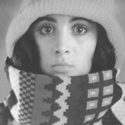
(a) Original trui.png image

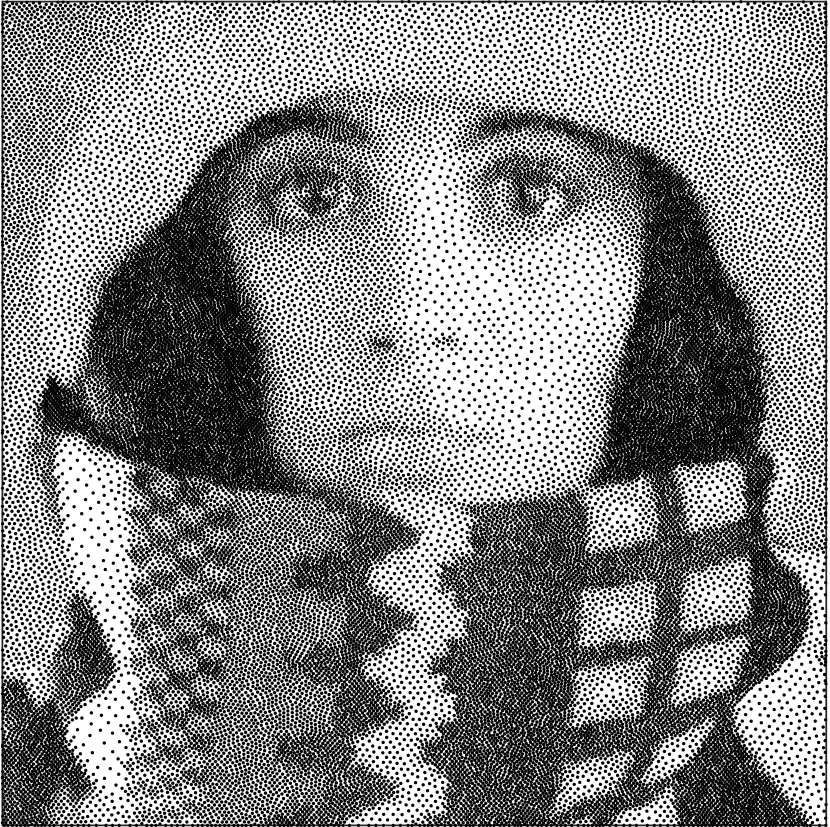
(b) Dithered trui image

Figure 3: The original trui.png image and a dithered version with 36,303 nodes, obtained by the algorithm in [46].

4.1 Heuristic Comparison

This section provides visualizations of the subsampled node sets of each algorithm. Each algorithm is applied twice to the dithered trui image as seen in Figure 4. The original node set contains 36303 nodes, the first subsample contains 10553 nodes, and the second subsample contains 3404 nodes. Each algorithm discussed, excluding the generalized diversity subsampling algorithm, requires a parameter, $c$, to control the level of coarsening. To reproduce the subsamples in Figure 4, the values of $c$ used in each algorithm are listed in Table 1. The moving front algorithm also relies on a choice of nearest neighbors which was $k=10$ for these tests.

Method	First Subsampling	Second Subsampling
MF	1.5101	1.518
W	3.44	3.1
PD	1.4931	1.5394

Table 1: The parameters, $c$, for reproducing the node sets in Figure 4 for the moving front (MF), weighted (W), and Poisson disk (PD) subsampling algorithms. The generalized diversity subsampling algorithm explicitly relies on the desired number of nodes in the coarse node set and thus has no parameter listed here. The moving front algorithm also relies on a choice of nearest neighbors which was $k=10$ for these tests.

A heuristic comparison between the subsamplings iterations primarily demonstrates the visual goodness of the first three algorithms over the generalized diversity subsampling algorithm. Among the remaining three, the woman’s nostrils are more distinct in the moving front and Poisson disk algorithms than in the weighted subsampling while the Poisson disk algorithm seems to preserve the mouth slightly more clearly by the second subsampling. Additionally, the moving front and Poisson disk algorithms preserve a higher level of clarity in the patterns in the trui scarf than the weighted subsampling algorithm. Again, the moving front and Poisson disk subsampling algorithms each better preserve the density disparity between areas of low and high node density in the original dithering than do the weighted or generalized diversity subsampling algorithms. Finally, the Poisson disk algorithm may have a tendency to subsample too aggressively in places. It should be noted that no direction bias of the moving front algorithm is visible.

Moving Front

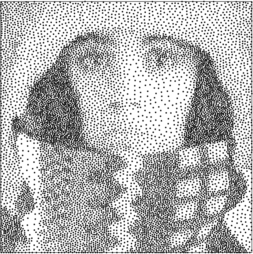
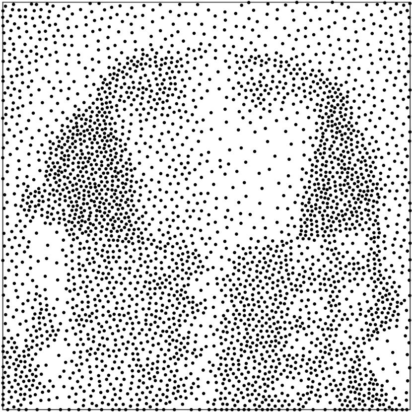
Weighted

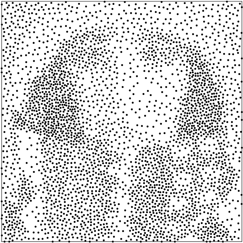
Poisson Disk

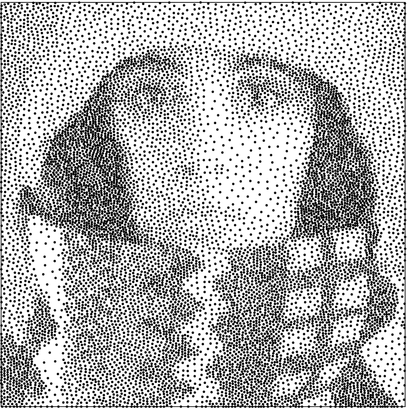
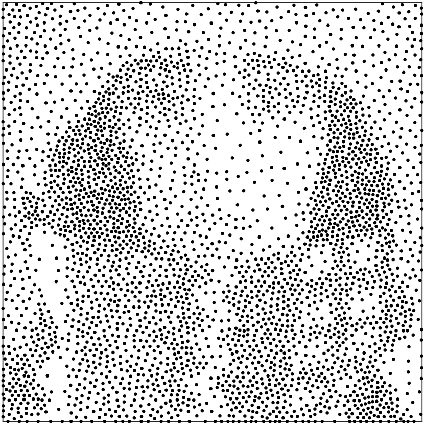
Generalized Diversity

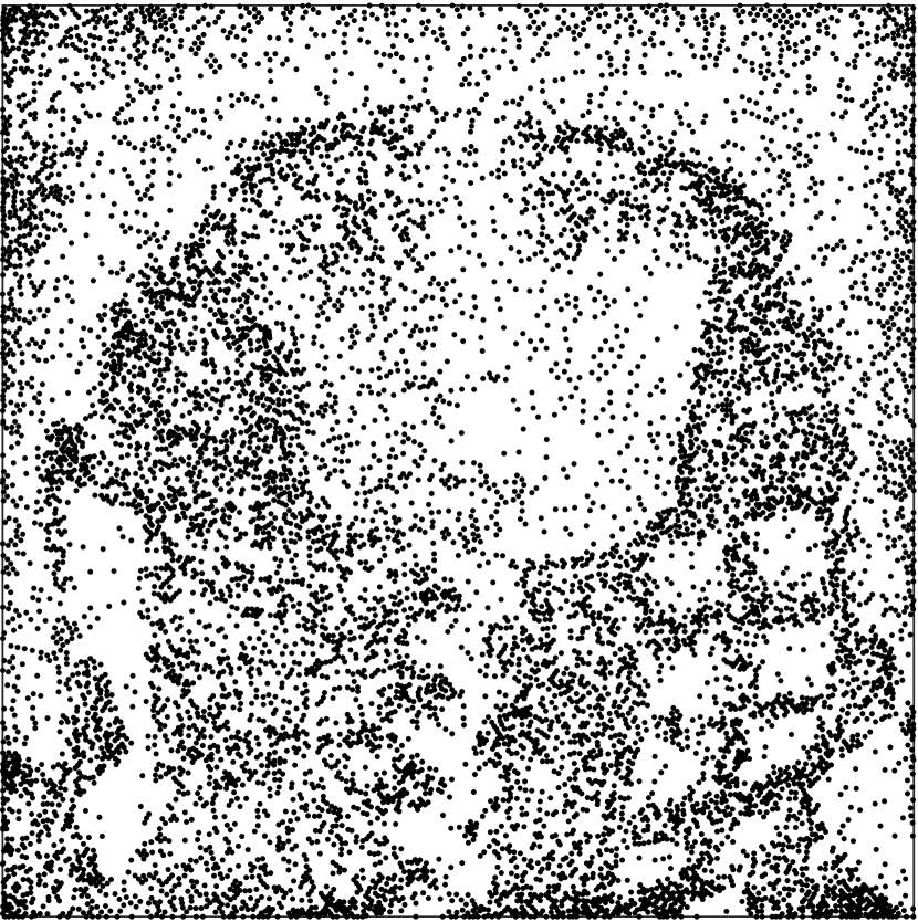
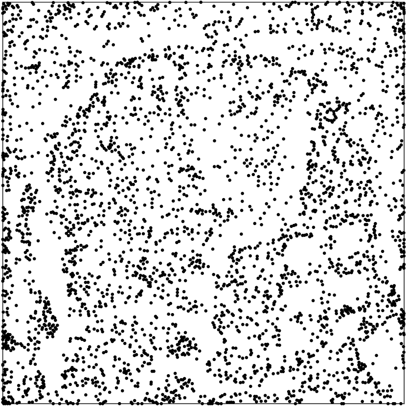
Figure 4: A visualization of the initial dithered trui image (36303 nodes), the first subsampling (10553 nodes), and the second subsampling (3404 nodes). From top to bottom, the rows demonstrate the moving front, weighted, Poisson disk, and generalized diversity subsampling algorithms. The first column of the figure contains a redundant image of the initial dithering for convenience in comparison.

4.2 Node Quality Measures

While visually comparing the results of each algorithm is useful, ultimately a more rigorous and quantitative comparison is desirable. As such, a variety of node quality measures are commonly discussed when comparing uniform subsampling methods [46, 38]. However, metrics which describe the quality of spatially variable node densities are less common [46]. One way of evaluating the quality of a variable density node set on its own is through local regularity distribution of distance to the nearest $k$ neighbors $\delta_{i,j}$, $i=1,2,...k$ for each node $x_{j}$.

It is here considered sufficient to expect the node generation algorithm to produce an initial node set which is sufficiently good. The responsibility of a subsampling algorithm is then to preserve the characteristics of the original node set. A natural way to determine how well any subsampling preserves the quality of the initial node set is to measure the coarse node set in comparison to the fine node set.

The two novel measures presented here are straightforward extensions of the commonly accepted measures of local regularity for evaluating the quality of variable density node sets and are referred to as measures of comparative local regularity (CLR). These CLRs contrast the average or standard deviation of distances to the $k$ nearest neighbors of the fine node set from those of the coarse node set. For each node set $X$, the Euclidian distance between each node $x_{j}\in X$ and its $k$ nearest neighbors is calculated as $\delta_{i,j}=\|x_{j}-x_{i,j}\|$. The average $\overline{\delta}_{j}$ or standard deviation $\sigma_{j}$ of these distances is then found for each node $x_{j}inX$. These are typical measures of local regularity. However, the present goal is measure how similar the initial and subsampled node sets are. To this end, the distributions of $\overline{\delta}_{j}^{\ \text{fine}}$ and $\overline{\delta}_{j}^{\ \text{coarse}}$ over each of the fine and coarse node sets, respectively, are first normalized to be between 0 and 1. Then the difference between these distributions is calculated at each of the nodes in the coarse node set and each of the collocated nodes in the fine node set. Finally, the standard $L_{2}$ norm is taken to produce a measure of CLR. The same process can be applied using the standard deviation $\sigma_{j}$ of those distances $\delta_{i,j}$.

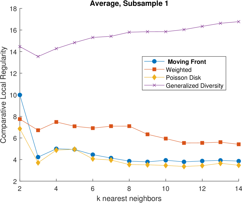
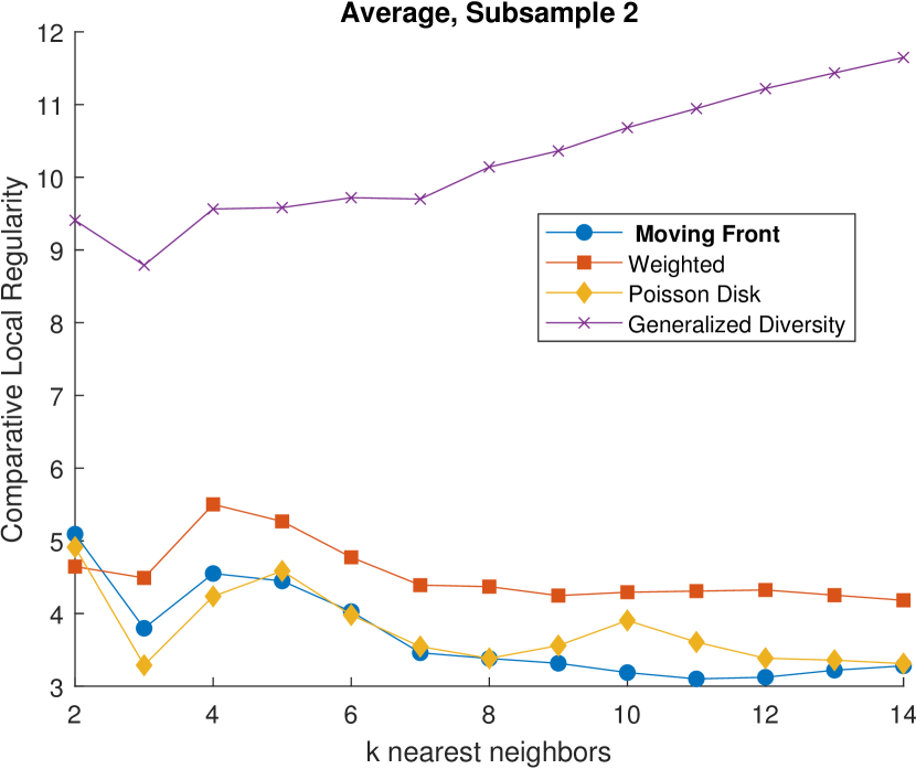
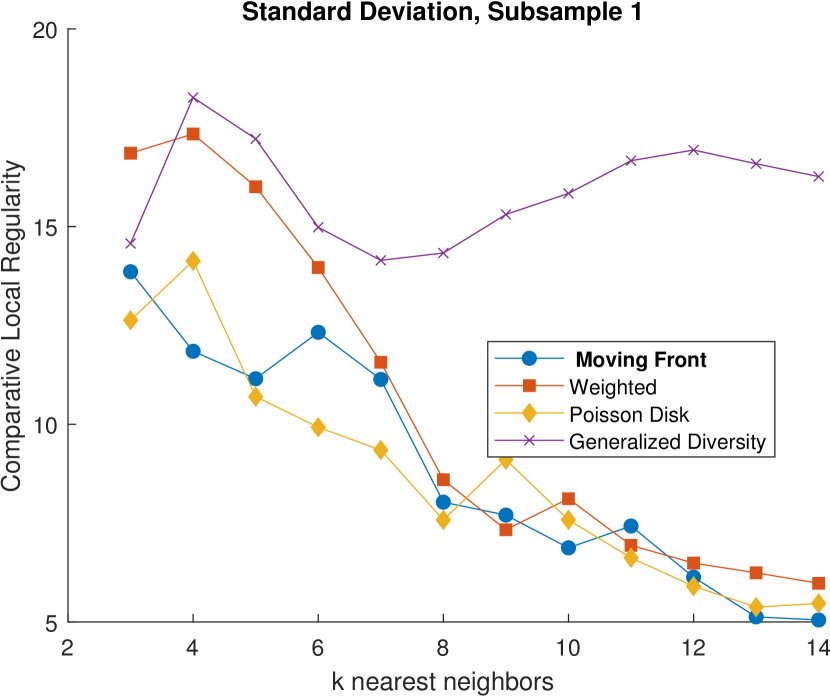
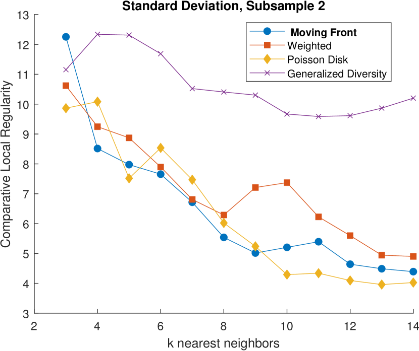
Figure 5: The comparative local regularity (CLR) of the average distance and standard deviation of distances for $k=2,3,...,14$ nearest neighbors of various subsampling methods (weighted, moving front, Poisson disk, and generalized diversity subsampling) applied once and twice to the dithered trui image. For both measures of CLR, a lower value is better.

Given that these CLRs measure the difference between a given initial node set and a subsampling of it, it is ideal to minimize these measures across algorithms. The presented CLRs should only be compared between subsamplings of the same size and from the same initial node set. Upon comparison of the average and standard deviation CLRs for each algorithm across various values of nearest neighbors as seen in Figure 5, it is clear that the moving front and Poisson disk algorithms preserve the characteristics of the initial dithered trui image better than the other two algorithms. This behavior is consistent across various sizes of node sets. Between them, however, it is not clear which one is qualitatively better.

4.3 Computational Cost

When evaluating any numerical scheme, computational cost must be considered as much as any other aspect of performance. The moving front, weighted, and Poisson disk subsampling algorithms presented in this paper were coded in MATLAB The generalized diversity subsampling algorithm is coded in Python as presented in [38]. A comparison of the computational complexity can be found in Figure 6. The average execution times in Figure 6 are calculated based on ten repetitions of each algorithm subsampling from the node set size of the previous data point to the node set size for the given point using the timeit commands native to MATLAB and Python. The moving front algorithm is clearly the fastest algorithm of those compared here. The significant computational cost savings secures the moving front algorithm as the best overall performing algorithm.

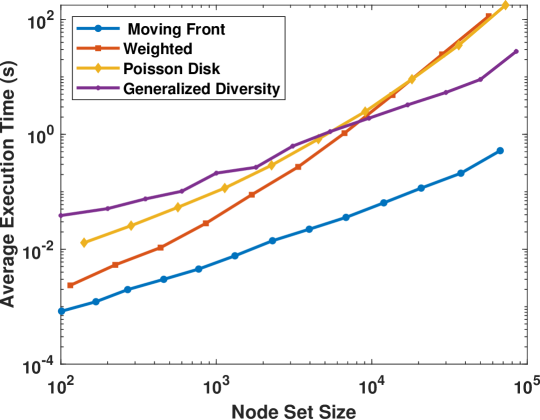
Figure 6: The computation time of each subsampling algorithm. The node set size is that of resultant subsample. Each subsample is subsequent such that the coarse node set of the previous iteration is the fine node set of the next. The execution time was averaged over ten iterations of the moving front, weighted, Poisson disk, and generalized diversity subsampling algorithms. Note the logarithmic scales. The moving front algorithm is significantly faster than any of the other algorithms.

5 Meshfree multilevel RBF-FD solver

Traditionally, multigrid solvers have been used to accelerate the solution of large systems of equations [5, 45]. Multigrid methods, however, require structured grids as the name indicates. In this section, it is illustrated how to utilize the geometric flexibility of RBF-FD in combination with the proposed node subsampling strategy to setup a geometric multilevel solver. Each example uses spatially varying node sets that seek to match the solutions. Consider the two-dimensional Poisson problem,

$$\mathcal{\nabla}^{2}u =f,\hskip 7.11317pt\bm{x}\in\Omega$$ (1)

$$u =g,\hskip 7.11317pt\bm{x}\in\partial\Omega$$

where $u=u(\bm{x})=u(x,y)\in\mathbb{R}$ is the exact solution in a disk with unit diameter, i.e., $\Omega=\{(x,y),x^{2}+y^{2}\leq 0.5\}$, $g=g(\bm{x})\in\mathbb{R}$ specifies Dirichlet boundary conditions on $\partial\Omega$ and $f=f(\bm{x})\in\mathbb{R}$ specifies the source term. Two different problems are solved using variable density node sets in order to test the applicability of the proposed node subsampling strategy. The first problem considered is the Poisson problem for which $g=0$ and $f=200e^{-100r}\left(100r-1\right)/r$ such that the solution given in polar coordinates is $u(r,\theta)=2\exp(-r/0.01)$, while the other is a Laplace problem (i.e. $f=0$) for which $g=\cos(10\theta)$ such that the solution given is $u(r,\theta)=1024\cos(10\theta)r^{10}$ (see Figure 7).

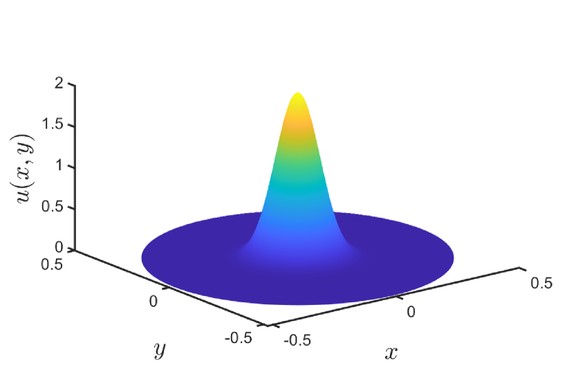
(a) $u(r,\theta)=2\exp(-r/0.01)$

(b) $u(r,\theta)=1024\cos(10\theta)r^{10}$

Figure 7: The analytical solutions used for the (a) Poisson and (b) Laplace test problems.

5.1 Radial basis function-generated finite differences

To discretize the problem in (1) using RBF-FD [1, 17, 20] we introduce the polyharmonic spline (PHS) radial basis functions $\phi_{i}(r)=\phi\left(\|\bm{x}-\bm{x}_{i}\|_{2}\right)=\|\bm{x}-\bm{x}_{i}\|_{2}^{2k+1}$ and bivariate monomials $p_{j}(\bm{x})$ to approximate the exact solution to (1) as

$$u(\bm{x})\approx u_{h}(\bm{x})=\sum_{i=1}^{n}\kappa_{i}\phi\left(\|\bm{x}-\bm{x}_{i}\|_{2}\right)+\sum_{j=1}^{\ell}\gamma_{j}p_{j}(\bm{x})$$ (2)

which we require to match at $n$ nodes, i.e., spatial points $\{\bm{x}_{i}\}_{i=1}^{n}$,

$$u(\bm{x}_{i})=u_{h}(\bm{x}_{i}),\hskip 7.11317pt\text{for}\hskip 7.11317pti=1,2,...,n,$$ (3)

while enforcing the additional constraints,

$$\sum_{i=1}^{n}\kappa_{i}p_{j}(\bm{x}_{i})=0,\hskip 7.11317pt\text{for}\hskip 7.11317ptj=1,2,...,\ell,$$ (4)

where $\ell=(m+1)(m+2)/2$ is the number of monomial terms in a bivariate polynomial of degree $m$. The above equations can be arranged in a linear system of equations,

$$\tilde{A}\begin{bmatrix}\bm{\kappa}\\ \bm{\gamma}\end{bmatrix}=\begin{bmatrix}A&P\\ P^{T}&0\end{bmatrix}\begin{bmatrix}\bm{\kappa}\\ \bm{\gamma}\end{bmatrix}=\begin{bmatrix}\bm{u}\\ \bm{0}\end{bmatrix},$$ (5)

where $\bm{\kappa},\bm{u}\in\mathbb{R}^{n}$, $\bm{\gamma}\in\mathbb{R}^{\ell}$, $A_{ij}=\phi\left(\|\bm{x}_{i}-\bm{x}_{j}\|_{2}\right)$ is an entry of the RBF collocation matrix $A\in\mathbb{R}^{n\times n}$ and $P_{ij}=p_{j}(\bm{x}_{i})$ is an entry of the supplementary polynomial matrix $P\in\mathbb{R}^{n\times\ell}$. Now, the linear operation $\mathcal{L}$ can be approximated at an evaluation point $\bm{x}_{e}$ as,

$$\mathcal{L}u|_{\bm{x}_{e}}\approx\sum_{i=1}^{n}\kappa_{i}\mathcal{L}\phi\left(\|\bm{x}-\bm{x}_{i}\|_{2}\right)|_{\bm{x}_{e}}+\sum_{j=1}^{\ell}\gamma_{j}\mathcal{L}p_{j}(\bm{x})|_{\bm{x}_{e}},$$ (6)

which again can be arranged in matrix-vector format,

$$\mathcal{L}u|_{\bm{x}_{e}}\approx\left[\bm{a}^{T}\hskip 5.69046pt\bm{b}^{T}\right]\begin{bmatrix}\bm{\kappa}\\ \bm{\gamma}\end{bmatrix}=\left[\bm{a}^{T}\hskip 5.69046pt\bm{b}^{T}\right]\tilde{A}^{\text{-}1}\begin{bmatrix}\bm{u}\\ \bm{0}\end{bmatrix}=\left[\bm{w}^{T}\hskip 5.69046pt\bm{v}^{T}\right]\begin{bmatrix}\bm{u}\\ \bm{0}\end{bmatrix}=\bm{w}^{T}\bm{u}$$ (7)

where $a_{i}=\mathcal{L}\phi\left(\|\bm{x}-\bm{x}_{i}\|_{2}\right)|_{\bm{x}_{e}}$ corresponds to the $i$th entry of $\bm{a}\in\mathbb{R}^{n}$ and $b_{j}=\mathcal{L}p_{j}(\bm{x})|_{\bm{x}_{e}}$ corresponds to the $j$th entry of $\bm{b}\in\mathbb{R}^{\ell}$. The weights necessary for the multilevel solver, i.e. $\bm{w}\in\mathbb{R}^{n}$, can equivalently be computed by solving the linear system,

$$\begin{bmatrix}A&P\\ P^{T}&0\end{bmatrix}\begin{bmatrix}\bm{w}\\ \bm{v}\end{bmatrix}=\begin{bmatrix}\bm{a}\\ \bm{b}\end{bmatrix}.$$ (8)

5.2 Geometric multilevel elliptic solver

The meshfree geometric multilevel solver introduced here is based on similar ideas as the meshfree geometric multilevel method [52] used for solving PDEs on surfaces, although some parts differ. In this study, no Krylov subspace methods will be used to increase the rate of convergence [21]. Furthermore, the coarse grid difference operators are computed explicitly on each node set level. Finally, all restriction operations are performed as injection (i.e. directly using values from the fine node set). For further details on multilevel methods, the reader is referred to literature on the topics of multilevel approximation [14, 49] and multilevel solvers [52, 54].

A pseudocode for the proposed geometric multilevel solver is given in Algorithm 2, where $u_{1}$ is the solution at the finest node set level, $L=\{L_{j}\}_{j=1}^{p}$ are the difference operators computed for each level, $I=\{I_{j+1}^{j}\}_{j=1}^{p-1}$ are the interpolation operators for each level and $R=\{R_{j}^{j+1}\}_{j=1}^{p-1}$ are the restriction (injection) operators for each level. The multilevel solver performs up to $i_{max}$ iterations (V-cycles) unless the relative residual $||r_{1}^{i}||_{2}/||r_{1}^{0}||_{2}=||f_{1}-L_{1}u_{1}^{i}||_{2}/||f_{1}-L_{1}u_{1}^{0}||_{2}$ of the $i$th iteration becomes less than a predefined tolerance $tol$.

The basis of the geometric multilevel solver is the geometric multilevel V-cycle, which is described in Algorithm 3. During the V-cycles, pre- and post smoothing operations are performed using $(\nu_{1},\nu_{2})$ Gauss-Seidel relaxations, respectively. At the coarsest node set level, a sparse LU solver is used.

The pseudocode for performing the geometric multilevel preprocessing, i.e., establishing all the different subsets of nodes, $X=\{X_{j}\}_{j=1}^{p}$, and the discrete operators $L,I,R$, is given in Algorithm 4. The necessary input for this algorithm are two node sets, $\{X_{bg},X_{b}\}$, which describe the scattered node set covering $\Omega$ and boundary nodes on $\partial\Omega$ at the finest node set level, respectively. Finally, the parameter $N_{\text{min}}$ is used to control the minimum number of boundary nodes at the coarsest node set level.

Algorithm 2 Geometric multilevel solver

1:function mlsolver($u_{1},f_{1},L,I,R,\nu_{1},\nu_{2},tol,i_{max}$)

2:    while $i<i_{max}$ and $||r_{1}||_{2}<||f_{1}||_{2}\cdot tol$ do

3:         $i\leftarrow i+1$

4:         $u_{1}\leftarrow\textsc{mlvcyc}(u_{1},f_{1},L,I,R,\nu_{1},\nu_{2})$

5:    end while

6:    return u

7:end function

Algorithm 3 Geometric multilevel V-cycle

1:function mlvcyc($u_{1},f_{1},L,I,R,\nu_{1},\nu_{2}$)

2:    $u_{1}\leftarrow\textsc{relax}(u_{1},f_{1},L_{1},\nu_{1})$

3:    $r_{2}\leftarrow R_{1}^{2}(f_{1}-L_{1}u_{1})$

4:    for $j=2$ to $p-1$ do

5:         $e_{j}\leftarrow\textsc{relax}(0,r_{j},L_{j},\nu_{1})$

6:         $r_{j+1}\leftarrow R_{j}^{j+1}(r_{j}-L_{j}e_{j})$

7:    end for

8:    $e_{p}=\textsc{lusolve}(L_{p},r_{p})$

9:    for $j=p-1$ to $2$ do

10:         $e_{j}\leftarrow e_{j}+I_{j+1}^{j}e_{j+1}$

11:         $e_{j}\leftarrow\textsc{relax}(e_{j},r_{j},L_{j},\nu_{2})$

12:    end for

13:    $u_{1}\leftarrow u_{1}+I_{2}^{1}e_{2}$

14:    $u_{1}\leftarrow\textsc{relax}(u_{1},f_{1},L_{1},\nu_{2})$

15:    return $u_{1}$

16:end function

Algorithm 4 Geometric multilevel preprocessing

1:function mlpre($X_{bg},X_{b},N_{\text{min}}$)

2:    $[X,R,p]\leftarrow\textsc{mlmfsub}(X_{bg},X_{b},N_{\text{min}})$

3:    $L_{1}\leftarrow\textsc{rbffd}(X_{1},X_{1})$

4:    for $j=1$ to $p-1$ do

5:         $I_{j+1}^{j}\leftarrow\textsc{rbffd}(X_{j+1},X_{j})$

6:         $L_{j+1}\leftarrow\textsc{rbffd}(X_{j+1},X_{j+1})$

7:    end for

8:    return $X,L,I,R,p$

9:end function

The multilevel solver is tested on node sets that have been generated with variable node densities as illustrated in Figure 8, where $N_{\text{min}}=60$ for the Poisson problem and $N_{\text{min}}=120$ for the Laplace problem. The node density function used in this study is defined by a linear transition between two prescribed node densities as,

$$\rho(d)=\begin{cases}\rho_{\text{1}},&d<d_{\text{lim}}\\ \rho_{\text{1}}+(\rho_{\text{2}}-\rho_{\text{1}})(d-d_{\text{lim}})/d_{\text{bl}},&d_{\text{lim}}\leq d\leq d_{\text{lim}}+d_{\text{bl}}\\ \rho_{\text{2}},&\text{otherwise}\end{cases}$$ (9)

where $d=||\bm{x}||_{2}$ is the distance to the origin according to Figure 7, $\rho_{\text{1}}$ is the node density in region 1, $d_{\text{lim}}$ is a distance within which $\rho_{\text{1}}$ is kept constant, whereas $d_{\text{bl}}$ is the distance over which $\rho_{\text{1}}$ linearly blends into $\rho_{\text{2}}$. It should be noted that the nodes in the vicinity of boundary have been adjusted by means of repulsion only at the finest node set level [18]. It should be noted that the node density function, $\rho(d)$, is chosen such that node density can be matched with the characteristics of the solutions.

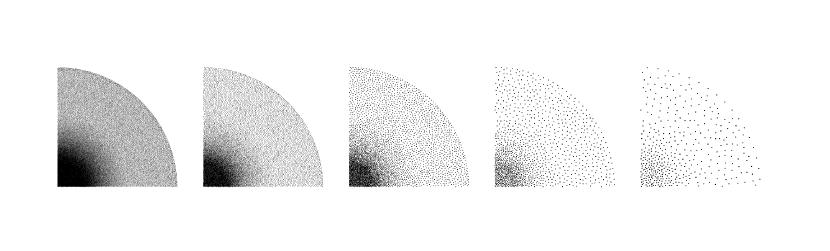
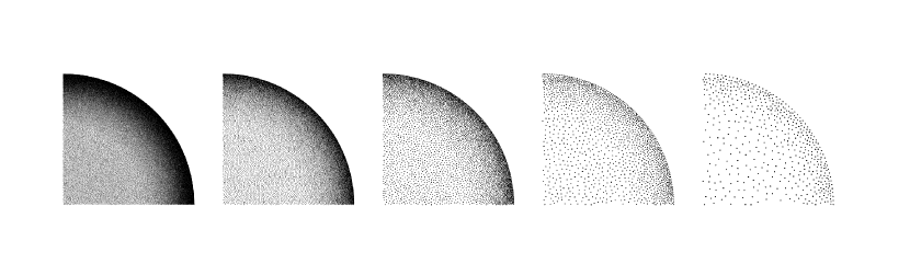
Figure 8: Example of the multilevel node subsampling process for the Poisson problem node set (top) and the Laplace problem node set (bottom). Only nodes within the first quadrant of the Cartesian coordinate system are shown.

The numerical test setups have been chosen to showcase the applicability of the node subsampling strategy for multilevel solvers using RBF-FD and to test whether the high-order accuracy will still be dictated by the degree of the augmented polynomials as shown, e.g., in [1]. Thus, the parameters used for computing the difference operators, $L$, of polynomial degree $m_{L}$ are chosen to be $(k,n)=(1,2\ell)$, while the parameters $(m_{I},k,n)=(0,0,5)$ are used for computing the interpolation operators, $I$. The parameters for the interpolation operators are kept fixed for all choices of $m_{L}$. Finally, the multilevel solver settings are defined as $(\nu_{1},\nu_{2},i_{max},tol)=(2,1,50,10^{-16})$ for both test problems, whereas the polynomial degree $m_{L}$ ranges from 2 to 8.

5.3 Poisson Equation Test Problem

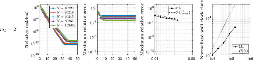
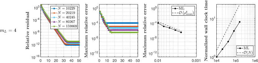
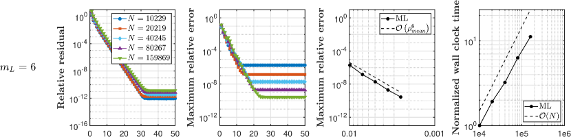
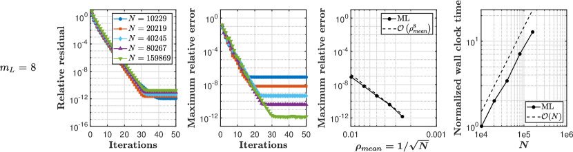
Figure 9: Poisson problem performance indicators of the implemented geometric multilevel solver for polynomial degrees of $m_{L}=\{2,4,6,8\}$ from top to bottom. The mean node density is defined as $\rho_{mean}=1/\sqrt{N}$.

First, it can be seen from Figure 9 that the wall clock time scales linearly with the number of nodes, which is in accordance with expectations for any multigrid or multilevel solver [5, 45, 52]. Furthermore, the maximum relative error ($||u-u_{h}||_{\infty}/||u||_{\infty}$) decreases as function of node set resolution ($\rho_{mean}=1/\sqrt{N}$) and the slope is dictated by the polynomial degree of the difference operator, $m_{L}$. This is in agreement with previous RBF-FD studies [1].

In this study, the low-order interpolation operators are chosen in order to accelerate the convergence of the multilevel solver. However, this choice is not aligned with the rule of thumb for the transfer operators, i.e. $m_{I}+m_{R}>2$, which is used in traditional multigrid methods for the Poisson problem [45]. In this work, the order of the restriction operators are $m_{R}=0$ because injection is used as the restriction operation between all node set levels. Nevertheless, no detrimental effects have been noticed in any of the numerical tests conducted.

Finally, the proposed multilevel solver should provide solutions without any directional bias. Hence, to identify whether any directional bias is present, the relative errors for all node set resolutions have been normalized and depicted in Figure 10. Thus, the scale factors used in Figure 10 refer to the plateau of the maximum relative error plots in Figure 9. As no particular directional pattern is noticed in Figure 10, it can be concluded that the subsampling process used for setting up the multilevel solver does not introduce any directional bias.

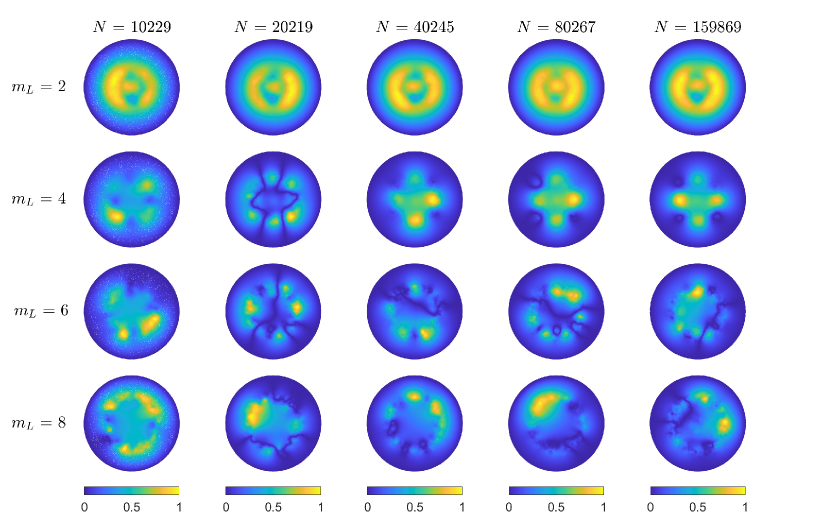
Figure 10: Normalized relative error distributions for various orders of the difference operators and node set resolutions for the Poisson problem. The color scale factors refer to the plateau of the maximum relative error plots in figure 9.

5.4 Laplace Equation Test Problem

The performance indicators of the multilevel solver for the Laplace problem are illustrated in Figure 11. The same overall conclusions that were made for the Poisson problem can be made for the Laplace problem, i.e. high-order accuracy and linear scaling of the computation time. For $m_{L}=8$, note that the convergence factor ($||r_{1}^{i}||_{2}/||r_{1}^{i-1}||_{2}$) of the multilevel solver is less for $N=14419$ and $N=28279$ compared with the other values of $N$. The decrease in convergence factors is most likely caused by a stencil size that is too large as compared to the relatively low node density near the boundary since localized error peaks are present for both $N=14419$ and $N=28279$ ($m_{L}=8$) in Figure 12. This decrease in convergence factor does not occur if the node resolution is increased to $N=55966$ or above. Furthermore, if the multilevel V-cycle is used as a preconditioner for a Krylov subspace method, e.g. the generalized minimal residual method or biconjugate gradient stabilized method, fewer iterations will be needed for the solution to converge and the solver will be more robust compared to the standalone multilevel solver. However, each iteration will become more computational expensive. Thus, whether the multilevel V-cycle should be used as a standalone solver or a preconditioner is a trade-off between computational cost and robustness.

The normalized relative error distributions in Figure 12 illustrate that no directional bias seems to be introduced by the subsampling process, which is the same conclusion as for the Poisson problem.

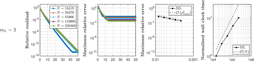
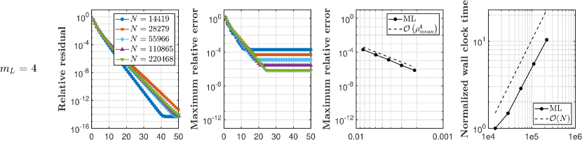
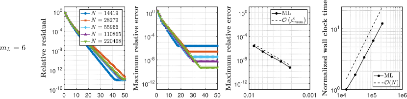
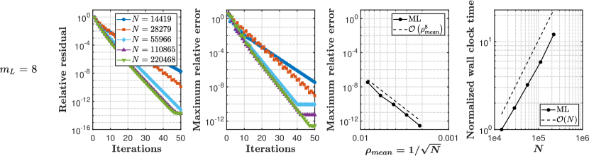
Figure 11: Laplace problem performance indicators of the implemented geometric multilevel solver for polynomial degrees of $m_{L}=\{2,4,6,8\}$ from top to bottom. The mean node density is defined as $\rho_{mean}=1/\sqrt{N}$.

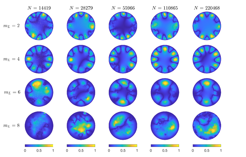
Figure 12: Normalized relative error distributions for various orders of the difference operators and node set resolutions for the Laplace problem. The color scale factors refer to the plateau of the maximum relative error plots in figure 11.

6 Conclusion

A novel method for subsampling quasi-uniform node sets of highly variable density with sharp gradients is presented along with boundary preservation techniques and two novel measures for evaluating node quality of subsamplings. The moving front subsampling algorithm demonstrates the capability to coarsen a node set with high contrast and detail. Additionally, the moving front algorithm maintains the characteristics of the original node set as outlined by the comparative local regularity of the average distance and standard deviation of distances to the $k$ nearest nodes. It is also faster, both by a constant and in the limit as node set size increases, than any other algorithm considered in this paper for subsampling variable density node sets.

The utility of the moving front algorithm for the purpose of subsampling node sets in a meshfree multilevel PDE solver is demonstrated by solving both the Poisson and Laplace problems on variable density node sets. In both test cases, the meshfree PDE solver with the multilevel method and the proposed subsampling algorithm achieves the fast linear scaling of computational cost with node set size expected from a multilevel scheme. At the same time, this combination has no adverse impact on the expected high-order accuracy of the RBF-FD method. The meshfree multilevel PDE solver has been tested up through eighth order convergence and also demonstrates very robust performance.

Acknowledgments: Andrew Lawrence acknowledges support from the US Air Force.

Appendix A Subsampling Algorithms

A.1 Moving Front Subsampling

The Python code for the moving front subsampling algorithm. The code can also be found on the author’s GitHub repository in both MATLAB and Python along with examples of implementation [26].

import numpy as np
from sklearn.neighbors import NearestNeighbors

def MFNUS(xy, fc=1.5, K=10):
    """
    Moving Front Non-Uniform Subsampling

    Args:
        xy (array): initial node set to be subsample
        c (float): coarsening factor
        K (float): number of nerarest neighbors to check in algorithm

    Returns:
        xy_sub (array): subsampled node set
    """
    if xy.shape[0] < xy.shape[1]:
        xy = xy.T

    # algorithm
    N = xy.shape[0]  # Get the number of its dots
    sort_ind = np.lexsort(xy.T,axis=0)
    xy = xy[sort_ind, :]  # Sort dots from bottom and up

    # Create nearest neighbor pointers and distances
    nbrs = NearestNeighbors(n_neighbors=K+1, algorithm=’auto’).fit(xy)
    distances, indices = nbrs.kneighbors(xy)

    for k in range(N):  # Loop over nodes from bottom and up
        if indices[k, 0] != N+1:  # Check if node already eliminated
            ind = np.where(distances[k, 1:] < fc*distances[k, 1])[0]
            ind2 = indices[k, ind+1]
            ind2 = np.delete(ind2,ind2 < k)   # Mark nodes above present one, and which
            indices[ind2, 0] = N+1        # are within the factor fc of the closest one

    elim_ind_sorted = indices[:, 0] != N+1
    xy_sub = xy[elim_ind_sorted]

    return xy_sub

References

- Bayona et al. [2017] V. Bayona, N. Flyer, B. Fornberg, and G. A. Barnett. On the role of polynomials in RBF-FD approximations: II. Numerical solution of elliptic PDEs. Journal of Computational Physics, 332:257–273, 2017.
- Behrens et al. [2001] J. Behrens, A. Iske, and S. Pöhn. Effective node adaption for grid-free semi-lagrangian advection. Discrete modelling and discrete algorithms in continuum mechanics, pages 110–119, 2001.
- [3] N. Bell, L. Olson, and J. Schroder. PyAMG: Algebraic Multigrid Solvers in Python. URL https://github.com/pyamg/pyamg.
- Bridson [2007] R. Bridson. Fast poisson disk sampling in arbitrary dimensions. SIGGRAPH sketches, 10(1):1, 2007.
- Briggs et al. [2000] W. L. Briggs, V. E. Henson, and S. F. McCormick. A Multigrid Tutorial. SIAM, second edition, 2000. doi: 10.1137/1.9780898719505.
- Cavoretto and De Rossi [2019] R. Cavoretto and A. De Rossi. Adaptive meshless refinement schemes for RBF-PUM collocation. Applied Mathematics Letters, 90:131–138, 2019.
- Cavoretto and De Rossi [2020] R. Cavoretto and A. De Rossi. A two-stage adaptive scheme based on RBF collocation for solving elliptic PDEs. Computers & Mathematics with Applications, 79(11):3206–3222, 2020.
- Cavoretto and De Rossi [2023] R. Cavoretto and A. De Rossi. An adaptive residual sub-sampling algorithm for kernel interpolation based on maximum likelihood estimations. Journal of Computational and Applied Mathematics, 418:114658, 2023.
- Cook [1986] R. L. Cook. Stochastic sampling in computer graphics. ACM Trans. Graph., 5(1):51–72, 01 1986. ISSN 0730-0301. doi: 10.1145/7529.8927.
- De Marchi et al. [2015] S. De Marchi, F. Piazzon, A. Sommariva, and M. Vianello. Polynomial meshes: Computation and approximation. In Proceedings of the 15th International Conference on Computational and Mathematical Methods in Science and Engineering, 2015.
- Dippé and Wold [1985] M. A. Z. Dippé and E. H. Wold. Antialiasing through stochastic sampling. SIGGRAPH Comput. Graph., 19(3):69–78, 07 1985. ISSN 0097-8930. doi: 10.1145/325165.325182.
- Drumm et al. [2008] C. Drumm, S. Tiwari, J. Kuhnert, and H.-J. Bart. Finite pointset method for simulation of the liquid–liquid flow field in an extractor. Computers & Chemical Engineering, 32(12):2946–2957, 2008.
- Falgout [2006] R. D. Falgout. An introduction to algebraic multigrid. Computing in Science and Engineering, vol. 8, no. 6, November 1, 2006, pp. 24-33, 4 2006.
- Fasshauer [2007] G. E. Fasshauer. Meshfree Approximation Methods with MATLAB, volume 6. World Scientific, 2007.
- Floater and Iske [1996] M. S. Floater and A. Iske. Multistep scattered data interpolation using compactly supported radial basis functions. Journal of Computational and Applied Mathematics, 73(1-2):65–78, 1996.
- Floater and Iske [1998] M. S. Floater and A. Iske. Thinning algorithms for scattered data interpolation. BIT Numerical Mathematics, 38:705–720, 1998.
- Flyer et al. [2016] N. Flyer, G. A. Barnett, and L. J. Wicker. Enhancing finite differences with radial basis functions: Experiments on the Navier-Stokes equations. Journal of Computational Physics, 316:39–62, 2016. ISSN 0021-9991. doi: https://doi.org/10.1016/j.jcp.2016.02.078.
- Fornberg and Flyer [2015a] B. Fornberg and N. Flyer. Fast generation of 2-D node distributions for mesh-free PDE discretizations. Computers & Mathematics with Applications, 69(7):531–544, 2015a. ISSN 0898-1221. doi: https://doi.org/10.1016/j.camwa.2015.01.009.
- Fornberg and Flyer [2015b] B. Fornberg and N. Flyer. Solving PDEs with radial basis functions. Acta Numerica, 24:215–258, 2015b. doi: 10.1017/S0962492914000130.
- Fornberg and Flyer [2015c] B. Fornberg and N. Flyer. A Primer on Radial Basis Functions with Applications to the Geosciences. SIAM, Philadelphia, PA, 2015c. doi: 10.1137/1.9781611974041.
- Ghai et al. [2019] A. Ghai, C. Lu, and X. Jiao. A comparison of preconditioned Krylov subspace methods for large-scale nonsymmetric linear systems. Numerical Linear Algebra with Applications, 26(1):e2215, 2019. doi: https://doi.org/10.1002/nla.2215. e2215 nla.2215.
- Ha and Choi [2021] S. T. Ha and H. G. Choi. A meshless geometric multigrid method based on a node-coarsening algorithm for the linear finite element discretization. Computers & Mathematics with Applications, 96:31–43, 2021.
- Kaennakham and Chuathong [2019] S. Kaennakham and N. Chuathong. An automatic node-adaptive scheme applied with a RBF-collocation meshless method. Applied Mathematics and Computation, 348:102–125, 2019.
- Katz and Jameson [2009] A. Katz and A. Jameson. Multicloud: Multigrid convergence with a meshless operator. Journal of Computational Physics, 228(14):5237–5250, 2009. ISSN 0021-9991. doi: https://doi.org/10.1016/j.jcp.2009.04.023.
- Kennard and Stone [1969] R. W. Kennard and L. A. Stone. Computer aided design of experiments. Technometrics, 11(1):137–148, 1969. doi: 10.1080/00401706.1969.10490666.
- [26] A. P. Lawrence. Subsampling algorithms. URL https://github.com/andplaw/Subsampling.
- Le Borne and Wende [2020] S. Le Borne and M. Wende. Multilevel interpolation of scattered data using H-matrices. NUMERICAL ALGORITHMS, 85(4):1175–1193, 12 2020. ISSN 1017-1398. doi: 10.1007/s11075-019-00860-1.
- Ling [2012] L. Ling. An adaptive-hybrid meshfree approximation method. International journal for numerical methods in engineering, 89(5):637–657, 2012.
- Liu and Platte [2021] T. Liu and R. B. Platte. Node generation for RBF-FD methods by QR factorization. Mathematics, 9(16), 2021. ISSN 2227-7390. doi: 10.3390/math9161845.
- Meng et al. [2022] X. Meng, Y. Li, D. Shi, S. Hu, and F. Zhao. A method of power flow database generation base on weighted sample elimination algorithm. Frontiers in Energy Research, 10, 2022.
- Metsch et al. [2020] B. Metsch, F. Nick, and J. Kuhnert. Algebraic multigrid for the finite pointset method. Computing and Visualization in Science, 23:1–14, 2020.
- Narayan and Xiu [2013] A. Narayan and D. Xiu. Constructing nested nodal sets for multivariate polynomial interpolation. SIAM Journal on Scientific Computing, 35(5):A2293–A2315, 2013. doi: 10.1137/12089613X.
- Nick [2020] F. P. Nick. Algebraic Multigrid for Meshfree Methods. PhD thesis, Universitäts-und Landesbibliothek Bonn, 2020.
- Oosterlee and Washio [1998] C. W. Oosterlee and T. Washio. An evaluation of parallel multigrid as a solver and a preconditioner for singularly perturbed problems. SIAM Journal on Scientific Computing, 19(1):87–110, 1998. doi: 10.1137/S1064827596302825.
- Piazzon et al. [2016] F. Piazzon, A. Sommariva, and M. Vianello. Caratheodory-Tchakaloff subsampling. Dolomites Research Notes on Approximation, 10, 11 2016.
- Roque et al. [2014] C. Roque, J. Madeira, and A. Ferreira. Node adaptation for global collocation with radial basis functions using direct multisearch for multiobjective optimization. Engineering Analysis with Boundary Elements, 39:5–14, 2014. ISSN 0955-7997. doi: https://doi.org/10.1016/j.enganabound.2013.10.012.
- Seibold [2010] B. Seibold. Performance of algebraic multigrid methods for non-symmetric matrices arising in particle methods. Numerical Linear Algebra with Applications, 17(2-3):433–451, 2010.
- Shang et al. [2022] B. Shang, D. W. Apley, and S. Mehrotra. Diversity subsampling: Custom subsamples from large data sets. 2022.
- Shapira [2008] Y. Shapira. Matrix-based multigrid: theory and applications. Springer, 2008.
- Silveira and Barbeira [2022] A. L. Silveira and P. J. S. Barbeira. A fast and low-cost approach for the discrimination of commercial aged cachaças using synchronous fluorescence spectroscopy and multivariate classification. Journal of the Science of Food and Agriculture, 102(11):4918–4926, 2022. doi: https://doi.org/10.1002/jsfa.11857.
- Sommariva and Vianello [2009] A. Sommariva and M. Vianello. Computing approximate Fekete points by QR factorizations of Vandermonde matrices. Computers & Mathematics with Applications, 57(8):1324–1336, 2009. ISSN 0898-1221. doi: https://doi.org/10.1016/j.camwa.2008.11.011.
- Suchde [2021] P. Suchde. A meshfree lagrangian method for flow on manifolds. International Journal for Numerical Methods in Fluids, 93(6):1871–1894, 2021.
- Suchde and Kuhnert [2019] P. Suchde and J. Kuhnert. A fully Lagrangian meshfree framework for PDEs on evolving surfaces. Journal of Computational Physics, 395:38–59, 2019.
- Suchde et al. [2022] P. Suchde, T. Jacquemin, and O. Davydov. Point cloud generation for meshfree methods: An overview. Archives of Computational Methods in Engineering, pages 1–27, 2022.
- Trottenberg et al. [2000] U. Trottenberg, C. W. Oosterlee, and A. Schuller. Multigrid. Elsevier, 2000.
- van der Sande and Fornberg [2021] K. van der Sande and B. Fornberg. Fast variable density 3-D node generation. SIAM Journal on Scientific Computing, 43(1):A242–A257, 2021.
- Volkov et al. [2016] K. N. Volkov, V. N. Emel’yanov, and I. V. Teterina. Geometric and algebraic multigrid techniques for fluid dynamics problems on unstructured grids. Computational Mathematics and Mathematical Physics, 56:286–302, 2016.
- Watanabe et al. [2005] K. Watanabe, H. Igarashi, and T. Honma. Comparison of geometric and algebraic multigrid methods in edge-based finite-element analysis. IEEE transactions on magnetics, 41(5):1672–1675, 2005.
- Wendland [2004] H. Wendland. Scattered Data Approximation, volume 17. Cambridge University Press, 2004.
- Wendland [2010] H. Wendland. Multiscale analysis in Sobolev spaces on bounded domains. Numerische Mathematik, 116:493–517, 2010.
- Wendland [2017] H. Wendland. Multiscale radial basis functions. In Frames and other bases in abstract and function spaces. Springer, 2017.
- Wright et al. [2023] G. B. Wright, A. Jones, and V. Shankar. MGM: A meshfree geometric multilevel method for systems arising from elliptic equations on point cloud surfaces. SIAM Journal on Scientific Computing, 45(2):A312–A337, 2023.
- Yuksel [2015] C. Yuksel. Sample elimination for generating Poisson disk sample sets. Computer Graphics Forum, 34:25–32, 5 2015. ISSN 1467-8659. doi: 10.1111/CGF.12538.
- Zamolo et al. [2019] R. Zamolo, E. Nobile, and B. Šarler. Novel multilevel techniques for convergence acceleration in the solution of systems of equations arising from RBF-FD meshless discretizations. Journal of Computational Physics, 392:311–334, 2019.
- Zhang et al. [2017] Q. Zhang, Y. Zhao, and J. Levesley. Adaptive radial basis function interpolation using an error indicator. Numerical Algorithms, 76:441–471, 2017.