Tuning Higher Order Structure in Colloidal Fluids

Abstract

Colloidal particles self assemble into a wide range of structures under AC electric fields due to induced dipolar interactions [Yethiraj and Van Blaaderen Nature 421 513 (2003)]. Tuning the external field drives structural transitions in the system. Here we consider colloidal fluids comprised of such dipolar particles in experiment and simulation and investigate their 2-body and higher-order structure using a variety of probes. The higher–order structure we probe using three-body spatial correlation functions and a many–body approach based on minimum energy clusters of a related system. These clusters exhibit a cascade of geometric transitions upon increasing the strength of the dipolar interaction, which are echoed in the higher–order structure of the concentrated fluids we study here.

I Introduction

Particles with a dipolar interaction are of great fundamental importance in the study of fluids and disordered materials. They are among the simplest models which describe long range directional interactions, which are exhibited by molecules  [1, 2]. Colloidal dispersions provide suitable models of atomistic and molecular systems as they exhibit phase behavior following the same rules of statistical mechanics, yet are amenable to real space observation using optical microscopy  [3, 4, 5]. Rather than spontaneous or intrinsic dipolar interactions as is often the case for atoms and molecules, in colloidal systems, dipoles are typically induced by an external electric or magnetic field  [4, 5, 6]. This has the consequence that the dipolar interactions are aligned in the direction of the electric field. In addition to their fundamental interest, such dipolar colloidal systems may find application as electrorheological fluids  [7, 8], hydraulic valves and photonic materials [9].

Among the attractions of dipolar colloidal systems is the ease with which the dipolar interactions can be tuned with the external field. Indeed real space studies of such systems led to the discovery of many crystal structures including fcc, hcp, bcc, body-centered tetragonal (bct) and body-centered orthorhombic (bco) structures  [10, 11, 5], along with a transient labyrinthine structure  [8]. Tuning the electric field in–situ enables the control of phenomena such as a martensitic transition  [12].

Adding softness  [13] or attractions  [14] to the interaction potential further increases the range of structures into which the system may self–assemble. In addition to the rich crystalline phase behavior, dipolar colloids feature a fluid phase at lower colloid volume fraction and electric field strength than those at which the crystals are found. In the colloidal fluid, as the field strength is increased, the symmetry–breaking dipolar interaction leads to a “string fluid” of particles organized in vertical lines [8, 10, 15], which can form the basis for producing “colloidal polymers” [16]. The emergence of this string fluid suggests a rather rich structure in the fluid. If characterized, such fluid structure could provide information on mechanisms by which nucleation in the polymorphic system might occur, due to the relation between fluid structure and crystallization [17, 18, 19].

Characterizing structure in the fluid state beyond pair correlations is challenging, although not impossible [20], and theoretical treatments have been developed for the higher–order structural of hard spheres [21, 22]. In experiment, particle–resolved studies of colloidal systems are ideal for studying higher–order structural correlations since particle–resolved data is amenable to the same kind of structural analyses as that of computer simulation, for which a number of methods have been developed [4].

Such methods include three–body correlation functions such as $g_{3}$ [21, 23, 24], and higher–order correlations such as common neighbor analysis (CNA)  [25] and Voronoi face analysis  [26] have shown to be successful in studying structures of fluids and glasses  [27, 28]. Another strategy, the bond orientation order (BOO) parameters developed by Steinhardt et al. steinhardt1983 [29], focuses on the local symmetry around a central particle. This method has been shown to be most successful in the study of crystallization, especially in identification of small crystalline clusters in a supercooled liquid[30, 31] and also in the characterization of fivefold symmetric order in amorphous systems  [32].

With the popularity of research in machine learning rising, it has been applied effectively to local structure in amorphous materials, for example by combining many structural metics such as the local pair correlation function  [33]. Other examples include combining it with local descriptors such as CNA and BOO to better characterize the local environment around a single particle in disordered materials  [34, 35]. Both supervised  [36] and unsupervised learning  [37] have been used to further our understanding of supercooled liquid and glass forming systems.

The methods listed above are geometric in nature. An alternative approach, which takes into account the interactions between the constituent particles of the system, has its roots in the work of Sir Charles Frank  [38], who postulated that since the minimum potential energy configuration of 13 Lennard-Jones atoms corresponds to an icosahedron, that this would be a common structure in (supercooled) liquids. With the advent of energy landscape calculations  [39], it has become possible to determine the structure of minimum potential energy clusters for a wide range and size of systems including the Lennard-Jones  [40] and Stockmayer  [41] models. The latter is a Lennard–Jones interaction with an additional dipolar interaction, which is not constrained to lie in any particular direction and thus corresponds to a molecular, rather than colloidal dipolar system in the context of the discussion above. While it is possible to determine minimum energy clusters, identifying local arrangements of particles in bulk systems whose bond network is identical to such clusters can be carried out using the topological cluster classification (TCC)  [42, 43]. The TCC has been used to identify locally favored structures or minimum energy clusters in systems undergoing dynamic arrest  [44], colloid-polymer mixtures interacting via Morse potential  [45], colloidal suspensions undergoing attractive interactions  [46], colloidal gels  [24, 47] and the liquid–gas interface  [48].

The colloidal dipolar system is interesting from the perspective of using minimum energy clusters to characterize the local structure because, unlike the systems mentioned above, the interaction potential is anisotropic and changes as a function of electric field strength. Some of us have recently determined the minimum energy clusters for the colloidal dipolar system [43], which opens the possibility to use this method to probe the higher–order structure of this system.

Herein, we report a combined experimental and computer simulation study of dipolar (nearly) hard sphere colloids in 3d with a range of methods of quantifying structure. We consider pair correlations in the form of radial distribution functions $g_{2}(r)$ and three-body correlations in the form of order parameters to determine “string-like” configurations and also a triplet correlation function $g_{3}(r,r^{\prime},\theta)$. Finally the we use the topological cluster classification  [42, 43] to explore higher–order spatial correlations. We find a good match between our experiment and simulation results. We also compared the Lennard-Jones–dipolar cluster populations present in experimental and simulation data with theoretical predictions from energy minimization calculations, since the topology of minimum energy clusters changes as a function of applied field strength [43].

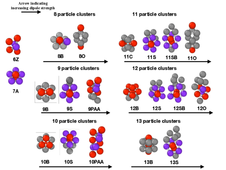
Figure 1: Minimum energy clusters of the dipolar–Lennard-Jones system for various sizes. Different geometries corresponds to a change in strength of the dipolar contribution.  [43].

II Dipolar Interactions in Colloidal Systems

The colloids in our experiments are immersed in an index-matching solvent with added salt, as described in Sec: III.1. The interaction between such colloids can be effectively modeled by a combination of a hard core Yukawa interaction [49, 50] and dipolar interaction [10]. The Yukawa term takes the from:

$$\beta u_{\mathrm{yuk}}(r) =\begin{cases}\infty&\mathrm{for}\ r\leq\sigma\\[2.00749pt] \beta\varepsilon_{\mathrm{yuk}}\frac{\exp\left(-\kappa(r_{ij}-\sigma\right)}{r/\sigma}&\mathrm{for}\ r>\sigma\end{cases}$$ (1)

where $\beta$ is the inverse of the thermal energy $k_{B}T$ with $k_{B}$ the Boltzmann constant, $T$ temperature, $u_{\mathrm{yuk}}$ the Yukawa interaction potential, $r$ the separation between two particles, $\sigma$ the hard-core particle diameter and $\kappa$ the inverse of the Debye screening length ($\kappa^{-1}=1/\sqrt{8\pi\lambda_{B}c}$ for monovalent salt).$\beta\varepsilon_{\mathrm{yuk}}$ is the potential at contact and can be expressed as:

$$\beta\varepsilon_{\mathrm{yuk}}=\frac{Z^{2}}{(1+\kappa\sigma/2)}\frac{\lambda_{B}}{\sigma}$$ (2)

where Z is the particle charge and $\lambda_{B}=e^{2}/4\pi\varepsilon_{0}\varepsilon_{m}k_{B}T$, the Bjerrum length of the suspending medium with dielectric constant $\varepsilon_{m}$. When colloids are subjected to external electric field, a dipole-dipole interaction is induced and the dipolar interaction takes the form

$$\beta u_{\mathrm{dip}}=\frac{\gamma_{\mathrm{exp}}}{2}\left(\frac{\sigma}{r}\right)^{3}\left(1-3{\left(\cos{\theta}\right)}^{2}\right)$$ (3)

where $u_{\mathrm{dip}}$ is the dipolar interaction, the $\theta$ is the angle made by $\mathbf{r}$ and the $z$-axis and $\gamma_{\mathrm{exp}}$ is a dimensionless prefactor that depends on the strength of the local external field.

$$\gamma_{\mathrm{exp}}=\frac{\mathbf{p}^{2}}{2\pi\varepsilon_{m}\varepsilon_{0}\sigma^{3}k_{B}T}$$ (4)

where

$$\mathbf{p}=\frac{\pi}{2}\beta\varepsilon_{m}\varepsilon_{0}\sigma^{3}\mathbf{E}_{\mathrm{loc}}$$ (5)

is the dipole moment. $\varepsilon_{m}$ is the dielectric constant of the suspending medium, $\varepsilon_{0}$ is the permittivity of vacuum and $\mathbf{E}_{\mathrm{loc}}$ is the local electric field.

Combining with the Yukawa interaction Eq. 1 the total interaction between two colloids under the electric field becomes:

$$\beta u_{\mathrm{total}}=\beta u_{\mathrm{dip}}+\beta u_{\mathrm{yuk}}.$$ (6)

III Methods

III.1 Experimental

The colloidal suspension used in this experiment was prepared by adding sterically-stabilized polymethyl methacrylate (PMMA) spheres (synthesized following reference  [51, 52]) ($\rho$ = 1.196 gcm^-3) [53] of diameter 1.73 $\mu$m (polydispersity=6.8%) in a mixture of density and refractive index matched organic solvents. The organic solvents consist of cis-decalin ($\rho$ = 0.897 gcm^-3) and cyclohexyl-Bromide (CHB) ($\rho$ = 1.32 gcm^-3). Tetrabutylammonium bromide (TBAB) was dissolved in the solvent to make up for a solution with TBAB salt concentration of 260 $\mu$M. This corresponds to a Debye length $\kappa^{-1}$ of around 100 nm  [54]. While more sophisticated treatments may be carried out to match the interaction potential  [54, 55], here we use a slightly soft potential in the computer simulations and presume this to be sufficient to match the experimental system, noting that the effects we seek to study are dominated by the dipolar interactions, rather than the hard core or precise colloid volume fraction (which we determine by weighing out the samples) [56].

In order to construct the electric cell to hold the colloidal suspension, two indium tin oxide glass slides were separated with spacer silica particles of approximately 60 $\mu$m in diameter to create a transparent, electrically conductive cell. The electrodes were connected to a signal generator that supplies alternating currents across the electrical cell.

A Leica SP8 confocal microscope was used to monitor colloidal assembly under the applied electric field. During each measurement, an entire stack of 3D confocal image of at least 200 “slices” of $xy$ images along the $z$ direction were taken with 256$\times$256 pixels with at least ten pixels per particle diameter in all directions. Only particles at least ten diameters from the wall were analyzed, to ensure that there were no significant wall effects. In each measurement, the applied voltage and the thickness of the electrical cell was measured in order to allow electric field strength comparison across different experiments. Before each measurement, the system is allowed to equilibrate for at least 20min. To obtain sufficient statistics at least 50 independent 3d images were taken.

III.2 Particle Tracking

The particle tracking was done via a custom written script to improve tracking accuracy of small particles in 3D (especially along the $z$-axis). It is effective in improving resolution of images that suffered from blurring in the axial direction [57]. The algorithm works by first finding some particles from a 3D image and obtaining their coordinates. From their coordinates, the average shape of the particles can be measured. With information on both positions and shape, the algorithm simulates some artificial images of the particles and compare them with the real images to identify previously unfound particles. Further details may be found in Ref.  [58]. can be tracked.

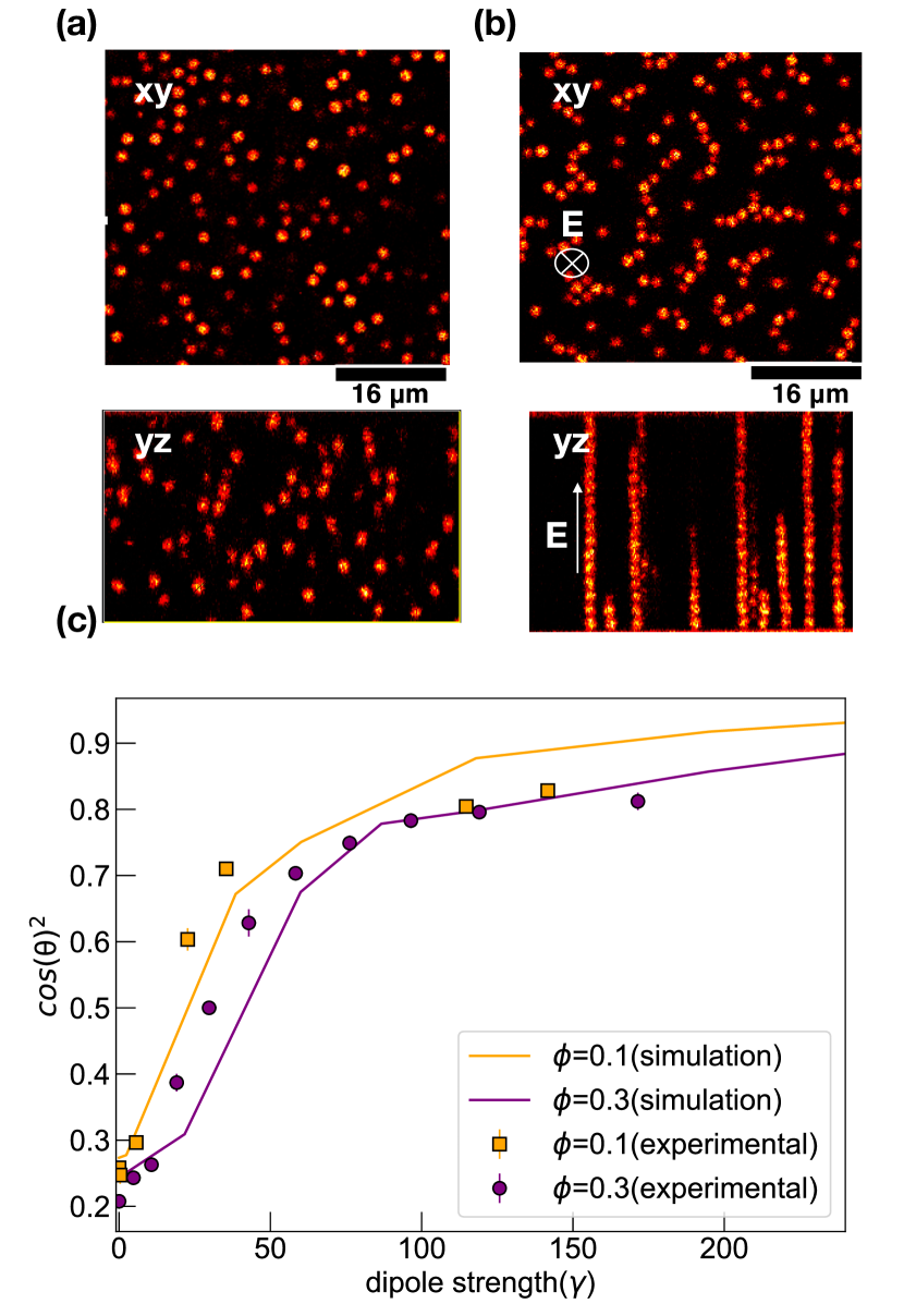
Figure 2: The colloidal dipolar system. (a) Representative images using confocal microscopy in the horizontal $xy$ and vertical $yz$ planes with no field, $\mathbf{E}=0$. Here volume fraction $\phi$=0.1. (b) Confocal microscopy images of a system at the same volume fraction at the maximum electric field strength 200 VMm^-1. (c) Bond order parameters (bop) (${\cos{\theta}}^{2}$) as a function of external electric field strength $E$. Data are shown for experiments and simulations as indicated in the legend.

III.3 Computer Simulation

We employed molecular dynamics simulations using the LAMMPS package at constant volume, in the NVT ensemble [59]. Similarly to reference [11], Ewald summation was used to compute long range dipole interactions in periodic boundary conditions. The system was evolved according to Brownian dynamics [60, 61]. Here we quote simulation results in reduced Lennard-Jones units. Each simulation run includes at least 3000 particles and was equilibrated for 1000 Lennard–Jones time units and sampled a further 100 time units. Effective volume fractions were determined with the Barker–Henderson effective hard sphere diameter.

We use a Weeks-Chandler-Anderson(WCA) interaction and added a dipole-dipole interaction shown in Eq. 3 to reproduce interactions in the experimental system. The WCA interaction takes the form:

$$\beta u_{\mathrm{wca}}(r_{ij}) =\begin{cases}\beta 4\varepsilon_{\mathrm{wca}}[(\frac{\sigma}{r})^{12}-(\frac{\sigma}{r})^{6}]+\varepsilon_{\mathrm{wca}}&\ r\leq 2^{\frac{1}{6}}\sigma\\[2.00749pt] 0&\ r>2^{\frac{1}{6}}\sigma\end{cases}$$ (7)

where $\varepsilon_{\mathrm{wca}}$ is the interaction energy. The interaction potential used in the computer simulations is then

$$\beta u_{\mathrm{sim}}=\beta u_{\mathrm{dip}}+\gamma_{\mathrm{sim}}\beta u_{\mathrm{wca}}.$$ (8)

where $\gamma_{\mathrm{sim}}$ controls the relative strength of the dipolar contribution and models the electric field strength in the experiments.

III.4 Bond order parameters for dipolar colloids

One method to quantify the angular correlation between particles as a function of external electric field strength is the bond order parameter (BOP). This has already been shown to be sensitive to variation in field strength by Li et al. [15]. These are calculated by finding the angle made by a reference particle with two of its nearest neighbor. For a system consisting of perfect chains, ${\cos^{2}\theta}$ = 1.

III.5 Two– and three–body correlation functions

The method described in the previous section offers a way of quantifying a change in structure for more dilute fluids. At higher concentration, we appeal at first to the two–body spatial correlation function, the radial distribution function $g_{2}(r)$. We also consider the 3–body spatial correlation function $g_{3}$. Now this is dependent on the correlations in positions of three particles, i.e. three vectors, eg $g_{3}(\mathbf{r}_{12},\mathbf{r}_{23},\mathbf{r}_{31})$ with the numbers reflecting the three particles. Here however we elect to simplify our representation to the case where we fix two of the distances (to the particle diameter $\sigma$) and vary the third separation between the particles, so that the 3–body correlation function is plotted as a function of angle between them $g_{3}(r_{12}=\sigma,{r}_{23}=\sigma,\eta)$ where $\eta$ is the angle between $\mathbf{r}_{12}$ and $\mathbf{r}_{23}$.

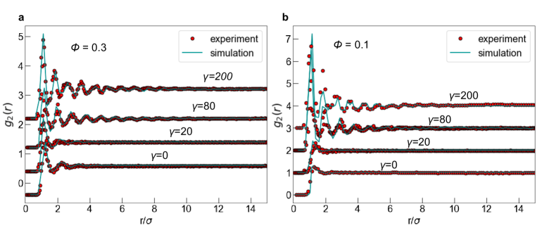
Figure 3: Radial distribution function ($g_{2}(r)$). Data are shown for both

experiment and computer simulations at volume fraction (a) $\phi=0.3$ and (b) $\phi=0.1$. Lines show different field strengths expressed through the parameter $\gamma$ as indicted. Data are offset for clarity.

III.6 Topological Cluster Classification

As discussed in the introduction, the topological cluster classification identifies local geometric motifs whose bond topology (defined here through a modified Voronoi decomposition) is identical to that of minimum energy clusters of a specific size [42]. These clusters are calculated from the energy optimization algorithm GMIN which uses basin-hoping to find local energetic minimum that corresponds to a specific configuration for an isolated number of particles[40]. Now such minimum energy clusters require an attractive interaction, and therefore to investigate the effect of the dipolar interaction, clusters were determined for a dipole added to a Lennard–Jones interaction  [43]. That is to say, the interaction potential for which the minimum energy clusters were determined was

$$\beta u_{\mathrm{tcc}}=\beta u_{\mathrm{li}}+\gamma_{\mathrm{tcc}}\beta u_{\mathrm{dip}}.$$ (9)

where $u_{\mathrm{lj}}$ is the Lennard–Jones interaction.

Those resulting clusters which turned out to be rigid  [43] are shown in Fig. 1 The clusters ending with PAA consist of 6Z clusters plus additional particles (9PAA and 10PAA). Whereas the S-clusters are built based on the 7A clusters (9S,10S,11S and 12S). The dipolar rigid clusters 8O, 9S, 9PAA, 10S, 10PAA, 11S, 11SB, 11O, 12S, 12SB, 12O and finally 13S are the minimum energy rigid clusters of particles interacting according to Eq. 9. In our analysis of the TCC clusters, we set the Voronoi parameter $f_{c}=0.82$ [42].

III.7 Orientation of anisotropic clusters

Since the dipolar interaction is anisotropic, the clusters found by the TCC may have a preferred orientation with respect to the direction of the electric field. We first isolated individual clusters found in both experiments and simulations. We calculated the principle axis of each cluster and determine the angle made by its principle axis with respect to the direction of the electric field. To quantify this angle distribution, we use an order parameter commonly used for liquid crystals,

$$\langle P_{2}(\cos\alpha)\rangle=\left\langle\frac{3}{2}\cos^{2}\alpha-\frac{1}{2}\right\rangle.$$ (10)

where $\alpha$ is the angle made by the principle axis of each cluster with the direction of the electric field  [62]. In the isotropic case when field is switched off, there should be no preferred orientation. In the perfectly aligned state, all the clusters should lie parallel to the electric field so this order parameter is $1$.

IV Results

We now present both experimental and simulation results for colloidal dipolar fluids at volume fractions $\phi=0.1$ and $\phi=0.3$. We investigate the bond order parameters, two and three body correlation functions, and populations of minimum energy clusters and the orientations of these clusters. These quantities are considered as a function of dipole strength $\gamma$. We convert external field strength to the dipole strength $\gamma$ using Eq. 4, which we use across experiments (Eq. 5), simulations (Eq. 8) and minimum energy clusters (Eq. 9).

IV.1 Bond order parameter analysis of the string fluid

In our study, with the bond order parameter (see Sec. III.6) we explored slightly higher volume fraction (0.1 and 0.3) than some previous work [15]. Our results are shown in Fig. 2 and we find rather good agreement between experiment and simulation. These show that at the range of volume fraction we are exploring the bond–order parameter analysis is not massively sensitive towards the change in volume fraction, with slightly higher values for the lower volume fraction system. However the BOP is highly sensitive to changes in external field strength. The general trend follows a sigmoid curve that exhibits a plateau at value close to unity.

IV.2 Two and three body correlation functions

Figure. 3 shows the $g(r)$ of both the computer simulations and experiments. We see that there is a good match between the two. As the dipole strength increases, the $g(r)$ reveals the emergence of relatively long range order.

In Fig. 4, we again show experimental and simulation results for the three–body correlation function $g_{3}$. Here the agreement between simulation and experiment is not as good as for the 2-body data described above, but we note that $g_{3}$ is of course higher order and more sensitive to small differences between the two.

At low field strength, a large and broad peak appears at approximately 60^∘ which is consistent with an isotropic system where interaction is angle independent[63]. As the field strength increases, peaks can be seen at approximately 60^∘, 120^∘ and 180^∘, with most triplets having angle close to 180^∘. This happens when the particles start to form strings.

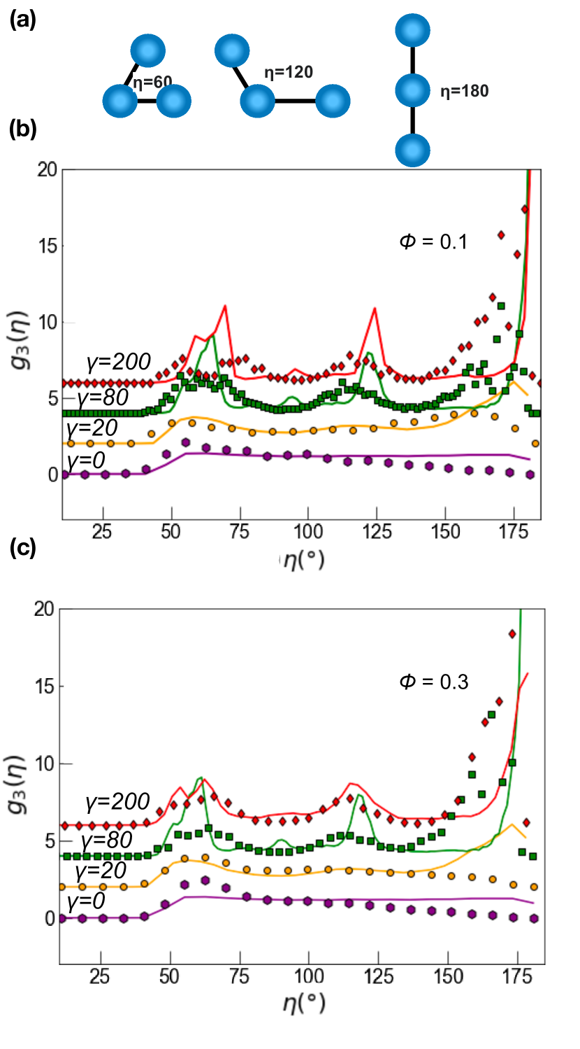
Figure 4: The three–body correlation function $g_{3}(\eta)$. (a) Schematic indications of geometries of interest, with values of the bond angle $\eta=$60^∘.120^∘ and 180^∘ (b) $g_{3}(\eta)$ is plotted for volume fraction $\phi=0.1$. (c) $g_{3}(\eta)$ for volume fraction $\phi=0.1$. In (b) and (c), data points are experimental data and lines are simulation data.

IV.3 Populations of minimum energy clusters

We now move to still higher–order spatial correlations and consider the minimum energy cluster geometric motifs identified by the topological cluster classification [43]. To facilitate comparison between experiment and simulation, we fix the number of particles in the cluster in question. Now the topology of the minimum energy cluster changes upon increasing the dipolar contribution [43]. In Fig. 5, we consider 8, 9 and 10–membered clusters, while in Fig. 6, data for larger 10 and 11–membered clusters is shown. Naively, one might expect that zero and low field strength would correspond to minimum energy clusters for the Lennard–Jones interaction as shown in Fig. 1 and known from studies with hard spheres [54, 47], and that upon increasing the field strength might lead to a cascade of clusters of increasing elongation as indicated in Fig. 1(b). Remarkably, this turns out to be the case.

For the smallest size of cluster which exhibits a non–trivial cascade of such clusters, $m=8$, indeed we see this trend with the Lennard–Jones minimum energy cluster 8B giving way to the dipolar cluster 8O for both volume fractions [Fig. 5(a,b)]. Notably, experiment and simulation appear rather well–matched here.

In the case of 9-particle clusters, a similar trend is found. In Fig. 5(c,d), we see clusters of 9B (the cluster expected for zero dipole strength) from $\gamma=0$ to $\gamma=29$, 9S from ($\gamma=29$ to $\gamma=50$), 9PAA from ($\gamma=50$ to $\gamma=87$ and finally strings at $\gamma>150$. The experimental and simulation work follow the same trends, with 9B peaking at $\gamma=0$, followed by 9S and finally 9PAA. Strings (which of course are non–rigid) overtake as the dominant cluster when $\gamma>150$. The analysis for strings is already considered in Sec. IV.1 where the maximum populations of strings occurred at the highest field strength with $\gamma>150$. Here, we see rather more clusters in the experimental data.

For the 10–membered clusters, again a cascade of cluster topologies is seen as a function of reduced field strength. In particular in Fig. 5(e,f), we see a transformation from the Lennard–Jones cluster 10B through 10S to 10PAA. The change in population correlates well with the values of dipole strength at which the topology of the minimum energy cluster varies. Here the agreement between experiment and simulation is less good, however the poorer statistics for these larger clusters as a source for this discrepancy cannot be ruled out.

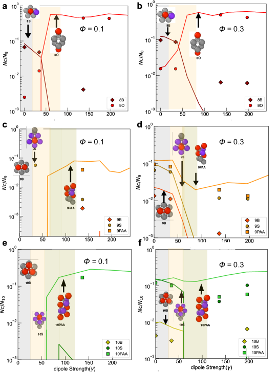
Figure 5: Populations of smaller minimum energy clusters detected by the topological cluster classification as a function of dipole strength. The number of particles detected in a given cluster $N_{c}$ is scaled by the number of particles in a cluster of that size. Shading denotes the change in cluster topology which minimizes the energy at different vales of the dipole strength $\gamma$ as indicated [43]. White regions of graphs denote values of $\gamma$ where the minimum energy clusters are not rigid. Data are shown for different cluster sizes $m$ and volume fractions as follows. (a) Cluster size $m=8$, volume fraction $\phi=0.1$. (b) $m=8$, $\phi=0.3$. (c) $m=9$, $\phi=0.1$. (d) $m=9$, $\phi=0.3$. (e) $m=10$, $\phi=0.1$. (f) $m=10$, $\phi=0.3$.

We now consider larger clusters in Fig. 6(a,b) for volume fraction 0.1 and 0,3 respectively. Data for $m=11$ are shown and here again the cascade of the Lennard–Jones 11C cluster being favored at zero and small field strength is found. This cluster topology gives way to 11S, 11SB and 11O upon increasing the dipole strength. For $m=11$ clusters, slightly more statistics are obtained for the experiments. Finally, for the $m=12$ data, the statistics are rather better for volume fraction $\phi=0.3$ in Fig. 6(d) than for $\phi=0.1$ in Fig. 6(c) and therefore we focus on $\phi=0.3$. Upon increasing the field strength, our simulations show a cascade from 12B (Lennard–Jones), through 12S, 12SB to 12O at higher field strength.

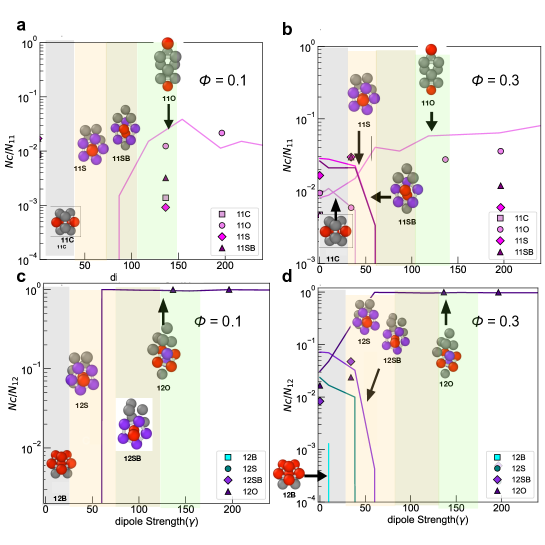
Figure 6: Populations of larger minimum energy clusters detected by the topological cluster classification as a function of dipole strength. As in Fig. 6, the number of particles detected in a given cluster $N_{c}$ is scaled by the number of particles in a cluster of that size. Shading denotes the change in cluster topology which minimizes the energy at different vales of the dipole strength $\gamma$ as indicated [43]. White regions of graphs denote values of $\gamma$ where the minimum energy clusters are not rigid. Data are shown for different cluster sizes $m$ and volume fractions as follows. (a) Cluster size $m=11$, volume fraction $\phi=0.1$. (b) $m=11$, $\phi=0.3$. (c) $m=12$, $\phi=0.1$. (d) $m=12$, $\phi=0.3$.

IV.4 Cluster Orientation

It is an interesting observation that even at zero dipole strength some minimum energy of dipolar clusters (such as 10PAA at $\phi=0.3$) are present in our system (Fig. 7). This enables us to investigate further into the orientation of these clusters using our method described above in Sec. III.7. Since the dipolar interactions of the individual particles are aligned along the direction of the electric field it is reasonable that the anisotropic clusters found by the TCC algorithm also show preferred orientation after the field is switched on. This we find for all the anisotropic clusters for which we have sufficient statistics, 8O, 9PAA, 9S, 10PAA, 11O and 12O as shown in Fig. 7.

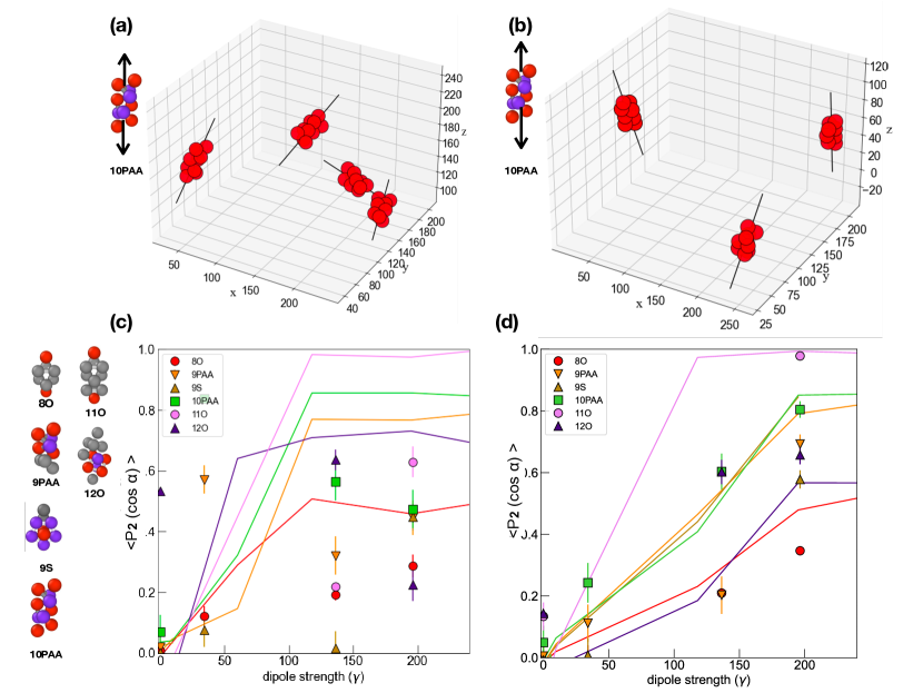
Figure 7: Orientation of anisotropic clusters with the electric field. (a) shows a 3D plot of the clusters (10PAA) found in the experimental dipolar colloids at $\phi=0.3$ at zero field, where the principal axis (shown in black line) of each cluster do not aligned with the electric field. Whereas in (b) these 10PAA clusters showed higher degree of alignment along E-field (z-axis) as field is switched on to $\gamma=240$. (c,d) $\langle P_{2}(\cos\alpha)\rangle$ of the principle axis is plotted as a function of reduced field strength, for the anisotropic clusters 8O, 9PAA, 9S , 10PAA, 11O and 12O. for the two volume fractions under consideration. (c) $\phi=0.1$ and (d) $\phi=0.3$. Data points are experimental data and lies are computer simulation.

V Discussion

We now discuss our findings figure by figure.

(i) Figure 2 shows confocal microscopy images of colloidal suspension of volume fraction, $\phi$=0.1, taken along the $xy$ plane (perpendicular to the direction of the electric field) and $yz$ plane (along the direction of field) for both zero dipole strength and at maximum dipole strength at $\gamma$=200. The dipolar colloids at $\gamma$=200 shows some structures with colloids forming strings along the direction of the field. Across the $xy$ plane, dipolar colloids show signs of aggregation, forming an almost labyrinth-like structure. Such a labyrinth-like structure has been found in some dipolar systems, especially in higher volume fraction, but is transient  [8], while our systems are in equilibrium to the best of our knowledge. Figure 2(c) shows a plot of bond order parameters of string from both our experiment and simulation results, similar to the study published by Li et al. [15]. Again, our simulations (line) and experiments (data points) show excellent agreement. As field strength increases, more dipolar colloids form strings and the angle made by colloids tends towards 180^∘. As indicated in Fig. 2(c), the degree of string formation increased gradually as opposed to a sharp increase like a step function.

(ii) In Fig. 3 we plot $g_{2}(r)$. This is generally in excellent agreement between computer simulations and experiments at for both $\phi$=0.3 and $\phi$=0.1 (with the only exception at $\phi$=0.1, $\gamma$=200). We can therefore be rather confident that the simulation model used in our work is a good reflection of our experimental system. The graphs also show the emergence of long range order as field strength is increased. This is expected since the confocal images show that as the fluid becoming more structured as the colloids aligned along the field when it is switched on. The height of the first peak of $g_{2}(r)$ also increases as field strength is increases, this means that the number of neighbors of each colloidal particle also increases as field is switched on. However, the above-mentioned changes in the plots are only applicable to higher field strength. At low field strength, between $\gamma$=0 to $\gamma$=50, there is barely any change in $g_{2}(r)$. The $g_{2}(r)$ is not able to distinguish minute changes to fluid. This is an important for our discussion below concerning the higher–order correlations detected by on $g_{3}$ and the TCC.

(iii) We now consider three–body correlations in Fig. 4. As the dipolar strength increases, the peak at 180^∘ increases as expected since more dipolar colloids form strings. However, we also observe peaks at 60^∘ and 120^∘ increasing with respect to field strength. This could correspond to the particle arrangements across the $xy$ plane where the labyrinth-like structure emerged. Even though $g_{3}$ is more sensitive than $g_{2}$ towards small structural variations in fluids, there is still very little variations between graphs at lower field strength. To identify small structural variation at lower field strength, we turn to the topological cluster classification.

(iv) The plots in Figures 5 and 6 show the population of dipolar clusters of different geometries and sizes analyzed with the TCC. In particular Fig. 5(a) and (b) show the population of clusters made of 8 particles; (c) and (d) show the population clusters made of 9 particles; (e) and (f) for 10 particle clusters. Figure 6 (a) and (b) shows data for 11 particle clusters while (c) and (d) concerns 12 particle cluster. In most cases, the cluster population found in experiment and simulation match.

Another observation which can be made from the graph is that the cluster topology changes at the dipole strength which corresponds to the minimum energy calculation  [43]. Minimum energy dipolar clusters are by definition at zero temperature, and are determined by the interaction energy. However, at finite temperature, entropy plays a role in many colloidal systems and its phase behavior is determined by a combination of energy and entropy. The fact that the cluster population trends largely follow the minimum energy clusters indicates that the behavior of dipolar colloids is influenced by energetics. This is in stark – and surprising – contrast to earlier work which suggested that energy plays only a very limited role in cluster populations  [45]. Presumably the strength of the dipolar interactions (which are much larger than eg Lennard–Jones interactions   [45]) is important here.

(v). Figure 7 shows that the anisotropic dipolar clusters tend to align along the $z$-axis (parallel with direction of the field) when it switched on. The $P_{2}(\cos{\theta})$ plot in Fig. 7(c) shows that as the field strength increases, so does the orientational order parameter $P_{2}$. $P_{2}$ has a maximum value of 1 which indicates when principle axes of clusters are parallel to the electric field. Our result also shows that more anisotropic, elongated clusters (e.g. 11O) have higher orientational order parameter $P_{2})$ than shorter clusters (e.g. 9S) at the same field strength.

Finally, we wish to discuss the importance of our results on the higher order fluid structures. A small variation in dipolar strength between $\gamma=0$ and $\gamma=30$ does not show up in $g_{2}(r)$ or even $g_{3}(r)$. Whereas, even at low field strength, dipolar clusters such as 8B and 8O populations vary drastically between different field strength (see Fig. 5). We can therefore conclude that higher order analysis such as that presented here is much more sensitive to small variation in structure and interactions. For instance, the TCC has already shown to be useful in analysis of glass transition and gel formation  [20, 44, 64].

Coupling our study with other previously published work on TCC analysis of gels and glasses  [64, 65], we can conclude that higher order structural analysis may be better at capturing the onset of phase transition than the standard $g_{2}(r)$. Furthermore the results showed that the string formation is not instantaneous. In fact, the degree of string formation increases gradually with field strength. This finding could be relevant for studies on electrorheological fluid where its structure is directly correlated with its physical properties such as viscosity and yield stress  [66]. Our result shows that potentially the external field strength could be used to control this fluid’s physical property to produce smart materials that respond to environmental changes reversibly.

VI Conclusion

We have performed a detailed analysis of the fluid structure in dipolar colloids and found good agreement between our experimensl and computer simulation data across a wide range of interactions tuned with the electric field. We found both bond–order parameter analysis of strings and the three–body correlation function $g_{3}$ to be suitable to quantify the degree of string formation in dipolar colloids but with $g_{3}$ offering more detailed information and can be used as a form of “colloidal finger-print” (analogous to infrared spectroscopy). With the topological cluster classification methods, not only can we identify clusters relevant to the dipolar colloids system but also isolate them to quantify their orientations with respect to field strength. Finally, our experimental and simulation work agrees with expectations from minimum energy clusters of a dipolar-Lennard-Jones system [43].

Data Availability Statement

Data and code available upon reasonable requests.

References

- Israelachvili [2011] J. N. Israelachvili, Intermolecular and Surface Forces, 3rd ed. (Academic Press, 2011).
- Gebbie et al. [2017] M. A. Gebbie, A. M. Smith, H. A. Dobbs, A. A. Lee, G. G. Warr, X. Banquy, M. Valtiner, M. W. Rutland, J. N. Israelachvili, S. Perkin, and R. Atkin, Chemical Communication 54, 1214 (2017).
- Evans et al. [2019] R. Evans, D. Frenkel, and M. Dijkstra M., Physics Today 72, 38 (2019).
- Ivlev et al. [2012] A. Ivlev, H. Löwen, G. E. Morfill, and C. P. Royall, Complex Plasmas and Colloidal Dispersions: Particle-resolved Studies of Classical Liquids and Solids (World Scientific Publishing Co., Singapore Scientific, 2012).
- Bharti and Velev [2015] B. Bharti and O. D. Velev, Langmuir 31, 7897 (2015).
- Donaldson et al. [2017] J. G. Donaldson, P. Linse, and S. S. Kantorovich, Nanoscale 9, 6448 (2017).
- Winslow [1949] Winslow, Journal of Applied Physics 20, 1137 (1949).
- Dassanayake et al. [2000] U. Dassanayake, S. Fraden, and A. van Blaaderen, J. Chem. Phys. 112, 3851 (2000).
- van Blaaderen [2004] A. van Blaaderen, MRS Bulletin 29, 85?90 (2004).
- Yethiraj and van Blaaderen [2003] A. Yethiraj and A. van Blaaderen, Nature 421, 513 (2003).
- Hynninen and Dijkstra [2005] A.-P. Hynninen and M. Dijkstra, Physical review letters 94, 138303 (2005).
- Yethiraj et al. [2004] A. Yethiraj, A. Wouterse, B. Groh, and van Blaaderen Alfons, Phys. Rev. Lett. 92, 058301 (2004).
- Colla et al. [2018] P. S. Colla, T. Mohanty, S. Nöjid, A. Riede, P. Schurtenberger, and C. Likos, ACS Nano (2018).
- Semwal et al. [2022] S. Semwal, C. Clowe-Coish, I. Saika-Voivod, and A. Yethiraj, Phys. Rev. X 12, 041021 (2022).
- Li et al. [2010] N. Li, H. Newman, M. Valera, I. Saika-Voivod, and A. Yethiraj, Soft Matter 6, 10.1039/B909953K (2010).
- Vutukuri et al. [2012] H. R. Vutukuri, A. F. Demirörs, B. Peng, P. D. J. van Oostrum, A. Imhof, and A. van Blaaderen, Angewandte Chemie International Edition 51, 11249 (2012).
- Gasser [2009] U. Gasser, J. Phys.: Condens. Matter 21, 203101 (2009).
- Russo and Tanaka [2012] J. Russo and H. Tanaka, Sci. Rep. 2, 505 (2012).
- Schillng et al. [2010] T. Schillng, H. J. Schoepe, M. Oettel, G. Opletal, and I. Snook, Phys. Rev. Lett. 105, 025701 (2010).
- Royall and Williams [2015] C. P. Royall and S. R. Williams, Phys. Rep. 560, 1 (2015).
- Hansen and McDonald [2006] J.-P. Hansen and I. R. McDonald, Theory of Simple Liquids, 3rd ed. (Chichester : Wiley, 2006).
- Robinson et al. [2019] J. F. Robinson, F. Turci, R. Roth, and C. P. Royall, Phys. Rev. Lett. 122, 068004 (2019).
- Russ et al. [2003] C. Russ, K. Zahn, and H. von Gruenberg, Journal of Physics:Condensed Matter 15 (2003).
- Royall et al. [2015a] C. P. Royall, J. Eggers, A. Furukawa, and H. Tanaka, Phys. Rev. Lett. 114, 258302 (2015a).
- Honeycutt and Andersen [1987] J. D. Honeycutt and H. C. Andersen, J. Phys. Chem. 91, 4950 (1987).
- Tanemura et al. [1977] M. Tanemura, Y. Hiwatari, H. Matsuda, T. Ogawa, N. Ogita, and A. Ueda, Progress of Theoretical Physics 58, 1079?1095 (1977).
- Jónsson and Andersen [1988] H. Jónsson and H. C. Andersen, Physical Review Letters 60, 2295 (1988).
- Bailey et al. [2004] N. P. Bailey, J. Schiøtz, and K. W. Jacobsen, Phys. Rev. B 69, 144205 (2004).
- Steinhardt et al. [1983] P. J. Steinhardt, D. R. Nelson, and M. Ronchetti, Phys. Rev. B 28, 784 (1983).
- Auer and Frenkel [2004] S. Auer and D. Frenkel, The Journal of Chemical Physics 120, 3015 (2004), https://doi.org/10.1063/1.1638740 .
- Kawasaki and Tanaka [2010] T. Kawasaki and H. Tanaka, Proceedings of the National Academy of Sciences 107, 14036 (2010).
- van Blaaderen and Wiltzius [1995] A. van Blaaderen and P. Wiltzius, Science 270, 1177 (1995).
- Cubuk et al. [2015] E. D. Cubuk, S. S. Schoenholz, J. M. Rieser, B. D. Malone, J. Rottler, D. J. Durian, E. Kaxiras, and A. J. Liu, Phys. Rev. Lett. 114, 108001 (2015).
- Boattini et al. [2020] E. Boattini, S. Marin-Aguilar, S. Mitra, G. Foffi, F. Smallenburg, and L. Filion, Nature Communication 11, 5479 (2020).
- Boattini et al. [2019] E. Boattini, M. Dijkstra, and L. Filion, Journal of Chemical Physics 151, 154901 (2019).
- Campos-Villalobos et al. [2021] G. Campos-Villalobos, E. Boattini, L. Filion, and M. Dijkstra, The Journal of Chemical Physics 155, 174902 (2021).
- Paret et al. [2020] J. Paret, R. L. Jack, and D. Coslovich, The Journal of Chemical Physics 152, 144502 (2020).
- Frank [1952] F. C. Frank, Proc. R. Soc. A. 215, 43 (1952).
- Wales [2004] D. J. Wales, Energy Landscapes: Applications to Clusters, Biomolecules and Glasses (Cambridge University Press, Cambridge, 2004).
- Wales and Doye [1997] D. J. Wales and J. P. K. Doye, Journal of Physical Chemistry A 101, 5111?5116 (1997).
- Miller and Wales [2005] M. A. Miller and D. Wales, J. Phys. Chem. B 109, 23109 (2005).
- Malins et al. [2013] A. Malins, S. R. Williams, J. Eggers, and C. P. Royall, Journal of Chemical Physics 139, 234506 (2013).
- Skipper et al. [2023] K. Skipper, F. J. Moore, and C. P. Royall, in preparation (2023).
- Royall et al. [2008] C. P. Royall, S. R. Williams, T. Ohtsuka, and H. Tanaka, Nature Mater. 7, 556 (2008).
- Taffs et al. [2010a] J. Taffs, A. Malins, S. R. Williams, and C. P. Royall, J. Phys.: Condens. Matter 22, 104119 (2010a).
- Taffs et al. [2010b] J. Taffs, A. Malins, S. R. Williams, and C. P. Royall, J. Chem. Phys. 133, 244901 (2010b).
- Royall et al. [2018] C. P. Royall, S. R. Williams, and H. Tanaka, J. Chem. Phys. 148, 044501 (2018).
- Godogna et al. [2010] M. Godogna, A. Malins, S. R. Williams, and C. P. Royall, Mol. Phys. 109, 1393 (2010).
- Royall et al. [2003] C. P. Royall, M. E. Leunissen, and A. van Blaaderen, J. Phys.: Condens. Matter 15, S3581 (2003).
- Royall et al. [2006] C. P. Royall, M. E. Leunissen, A.-P. Hyninnen, M. Dijkstra, and A. van Blaaderen, J. Chem. Phys. 124, 244706 (2006).
- Campbell and Bartlett [2002] A. I. Campbell and P. Bartlett, J. Coll. Interf. Sci. 256, 325 (2002).
- Hollingsworth et al. [2006] A. Hollingsworth, W. Russel, C. van Kats, and A. van Blaaderen, in APS March Meeting Abstracts, APS Meeting Abstracts (2006) p. G21.005.
- Royall et al. [2005] C. P. Royall, R. van Roij, and A. van Blaaderen, J. Phys.: Condens. Matter 17, 2315 (2005).
- Taffs et al. [2012] J. Taffs, S. R. Williams, H. Tanaka, and C. P. Royall, Soft Matter 9, 297 (2012).
- Royall et al. [2013] C. P. Royall, W. C. K. Poon, and E. R. Weeks, Soft Matter 9, 17 (2013).
- Poon et al. [2012] W. C. K. Poon, E. R. Weeks, and C. P. Royall, Soft Matter 8, 21 (2012).
- Cole et al. [2011] R. W. Cole, T. Jinadasa, and C. M. Brown, Nature Protocols 6, 1929?1941 (2011).
- Yang [2021] Y. Yang, nplocate, https://github.com/yangyushi/nplocate (2021).
- Plimpton [1995] S. Plimpton, Journal of Computational Physics 117, 1 (1995).
- Moore et al. [2021] F. J. Moore, C. P. Royall, T. B. Liverpool, and J. Russo, The European Physical Journal E 44, 121 (2021).
- Moore et al. [2023] F. J. Moore, R. J., T. B. Liverpool, and C. P. Royall, J. Chem. Phys. 158, 104907 (2023).
- Selinger [2016] J. V. Selinger, Liquid crystals, in Introduction to the Theory of Soft Matter: From Ideal Gases to Liquid Crystals (Springer International Publishing, Cham, 2016) pp. 131–182.
- Coslovich [2013] D. Coslovich, The Journal of Chemical Physics 138, 12A539 (2013), https://doi.org/10.1063/1.4773355 .
- Royall et al. [2015b] C. P. Royall, A. Malins, A. J. Dunleavy, and R. Pinney, Journal of Non-Crystalline Solids 407, 34 (2015b).
- Royall and Malins [2012] C. P. Royall and A. Malins, Faraday Discussion 158, 301 (2012).
- Wen et al. [2003] W. Wen, X. Huang, K. L. Shihe Yang, and P. Sheng, Nature Materials 2, 727 (2003).