Robust Data-Driven Safe Control
using Density Functions

Abstract

This paper presents a tractable framework for data-driven synthesis of robustly safe control laws. Given noisy experimental data and some priors about the structure of the system, the goal is to synthesize a state feedback law such that the trajectories of the closed loop system are guaranteed to avoid an unsafe set even in the presence of unknown but bounded disturbances (process noise). The main result of the paper shows that for polynomial dynamics, this problem can be reduced to a tractable convex optimization by combining elements from polynomial optimization and the theorem of alternatives. This optimization provides both a rational control law and a density function safety certificate. These results are illustrated with numerical examples.

1 Introduction

The goal of this paper is to develop a tractable framework for data-driven synthesis of safe control laws that are robust to $L_{\infty}$-bounded noise in both data-collection and during execution. Specifically, given noisy experimental data generated by an unknown system and some priors about its structure, the objective is to synthesize a state feedback law such that the trajectories of the closed loop system starting in a given initial condition set $\mathcal{X}_{0}$ are guaranteed to avoid an unsafe set $\mathcal{X}_{u}$, even in the presence of unknown but bounded disturbances. Our main result shows that, for polynomial dynamics, the safe Data Driven Control (DDC) problem can be posed as the feasibility of a Sum of Squares (SOS) program. A substantial reduction in the number of variables involved (and hence computational complexity) is achieved by exploiting the theorem of alternatives, leading to a Semidefinite Program (SDP) that provides both a density-function based control law and a robust safety certificate.

Safety verification and synthesis of safe control laws have been the subject of intense research during the past decade. Level-set methods separate the initial and unsafe set by the $0$-contour of a solved function. Barrier functions [1] are a level-set method to certify the safety of trajectories, given that the superlevel sets of the barrier function are invariant. This superlevel invariance can be relaxed through slack (class-$\mathcal{K}$) conditions, while ensuring that the $0$-level set is invariant [2, 3]. The level-set certificate of stability may be solved jointly with a safety-guaranteeing control policy $u(\cdot)$ ( Control Barrier Function (CBF)). When a barrier function is given, the min-norm controller will ensure safety of trajectories, and can be found through quadratic programming [4]. Robustness of given barrier functions to disturbances may be analyzed using input-to-state stability [5]. Barrier functions and funnels [6] contain bilinearities when jointly synthesizing controllers and barriers. An alternative level-set certificate is Density [7] functions, which are based on Dual Lyapunov methods for stability [8]. Controllers and density functions can be simultaneously solved in a convex manner. In some systems, density functions may exist and provide improved performance as compared to barrier functions [9].

We briefly compare against other methods of safety-constrained control. Interval analyses, such as Mixed Monotonicity [10], offer real-time performance at the expense of conservatism in safe generation. Hamilton-Jacobi reachability [11] performs forward and backward reachable set analysis based on level sets of a differential games’ value function, whose computation could require solving PDEs or neural net approximations. Reinforcement Learning necessitates training and prior information of safety properties (e.g. Lipschitz bounds on dynamics), and does not generally exploit physical principles and model structure [12]. Koopman methods leverage the predictive capabilities of nonlinear models, but they contain error bounds that can conflict against safety certification [13].

DDC is a methodology that synthesizes control laws directly from acquired system observations and skips a system-identification/robust-synthesis pipeline [14]. Amongst the vast literature in DDC, the closest approaches related to the present paper are those that pursue a set membership approach, which seeks to find a controller that stabilizes the set of all plants compatible with the observed data (the consistency set) [15, 16, 17, 18, 19, 20, 21, 22]. These approaches provide a controller together with a stability certificate, usually in the form of a common Lyapunov function. Further, the methods can be extended to provide worst case performance bounds (e.g. the $H_{2},H_{\infty}$ or $L_{\infty}$ sense), over the set of data-consistent plants. However, these approaches cannot handle safety constraints beyond those expressed in terms of these norms.

Recent work on DDC under safety constraints includes [23, 24, 25]. The method in [23] performs iterative model predictive control for a discrete-time system by constraining state trajectories to always lie in a sampled safe set (using integer programming). The work in [24] uses contraction methods to form robust adaptive CBFs under a set membership approach, but assumes that the input relation $g(\cdot)$ is known. The approach in [25] uses a disturbance observer to provide robust CBFs by separating known and unknown dynamics. In our setting, we assume only prior knowledge of the system model (polynomial up to a specified degree) and cannot generally provide this separation. Our work involves continuous-time dynamics and interpretable (density) certificates of robust safety. To the best of our knowledge, our approach is the first DDC method under safety constraints that simultaneously considers data-collection and online-dynamics noise.

Contributions of this work are,

• A DDC framework for density-based robust safe control.

• Tractable synthesis of robustly safe density functions by exploiting the theorem of alternatives.

• Numerical examples demonstrating robustly safe control on polynomial systems.

This paper has the following structure: Section 2 reviews preliminaries such as notation, density functions for safety, and SOS polynomials. Section 3 performs data-driven synthesis of safe controllers using density functions and SOS methods in the case where $L_{\infty}$-bounded noise occurs at data collection and the dynamics are subject to unknown but bounded disturbances. Section 4 demonstrates the effectiveness of our approach on several example systems. Section 5 concludes the paper.

2 Preliminaries

CBF

Control Barrier Function

DDC

Data Driven Control

LMI

Linear Matrix Inequality

LP

Linear Program

SDP

Semidefinite Program

SOS

Sum of Squares

2.1 Notation

$\mathbb{R}^{n}$	Set of $n$-tuples of real numbers
$x,{{\mathbf{x}}},{{\mathbf{X}}}$	Scalar, vector, matrix
$\mathbf{1,0},{{\mathbf{I}}}$	Vector/matrix of all 1s, 0s, identity matrix
$\left\|{{\mathbf{x}}}\right\|_{\infty}$	$L_{\infty}$-norm of vector ${{\mathbf{x}}}$
${{\mathbf{X}}}\succeq 0$	${{\mathbf{X}}}$ is positive semi-definite
$\otimes$	Kronecker product
vec$({{\mathbf{X}}})$	Vectorized matrix along columns:
	$\text{vec}({{\mathbf{X}}})=\left[{{\mathbf{X}}}(\colon,1)^{T},\ldots,{{\mathbf{X}}}(\colon,n)^{T}\right]^{T}$
$\rho\in C^{d}$	$\rho$ has a continuous $d^{th}$ derivative
$\nabla\rho$	Gradient of scalar function $\rho$
$\nabla\cdot f$	Divergence of vector function $f$

2.2 Sum-of-Squares

We briefly review the concept of SOS polynomials and proofs of nonnegativity [26]. A polynomial $p\in\mathbb{R}[{{\mathbf{x}}}]$ is SOS (and hence nonnegative) if there exist polynomials $\{q_{\ell}\in\mathbb{R}[{{\mathbf{x}}}]\}_{\ell=1}^{L}$ such that $p({{\mathbf{x}}})=\sum_{\ell=1}^{L}q_{\ell}({{\mathbf{x}}})^{2}$.

The cone of SOS polynomials is $\Sigma[{{\mathbf{x}}}]$, and its up to degree $2d$ restriction is $\Sigma_{d}[{{\mathbf{x}}}]$. The cone $\Sigma_{d}[{{\mathbf{x}}}]$ is semidefinite representable as $p({{\mathbf{x}}})={{\mathbf{v}}}({{\mathbf{x}}})^{T}{{\mathbf{Q}}}{{\mathbf{v}}}({{\mathbf{x}}})$ where ${{\mathbf{v}}}({{\mathbf{x}}})$ is the monomial vector up to degree $d$ and ${{\mathbf{Q}}}\succeq 0$ is the Gram matrix. A sufficient condition for a polynomial $p$ to be nonnegative over the semialgebraic region $\{{{\mathbf{x}}}\mid h_{i}({{\mathbf{x}}})\geq 0,\ i=1..N_{c}\}$ is that $p$ is contained in the quadratic module formed by $h_{i}$ (there exists $\sigma_{0..N_{c}}\in\Sigma[{{\mathbf{x}}}]$ such that $p({{\mathbf{x}}})=\sigma_{0}+\sum_{i=1}^{N_{c}}\sigma_{i}h_{i}$).

2.3 Level-Set-Based Safety Certification

Consider a continuous-time system of the form

$$\dot{{{\mathbf{x}}}}=f({{\mathbf{x}}},{{\mathbf{w}}})$$ (1)

where ${{\mathbf{x}}}\in\mathbb{R}^{n}$ is the state and ${{\mathbf{w}}}\in\mathcal{W}\subseteq\mathbb{R}^{n}$ is a disturbance. Further, assume that ${{\mathbf{w}}}(t)$ is such that the trajectories of (1) are well defined for any initial condition ${{\mathbf{x}}}_{0}\in\mathcal{X}_{0}$. In the sequel, we will denote these trajectories as ${{\mathbf{x}}}(t,{{\mathbf{w}}},{{\mathbf{x}}}_{0})$.

Definition 1.

Given an initial condition set $\mathcal{X}_{0}\subseteq\mathbb{R}^{n}$ and an unsafe set $\mathcal{X}_{u}\subseteq\mathbb{R}^{n}$, system (1) is robustly safe if, for all $t$, all initial conditions ${{\mathbf{x}}}_{0}\in\mathcal{X}_{0}$ and all ${{\mathbf{w}}}(t)\in\mathcal{W}$, ${{\mathbf{x}}}(t,{{\mathbf{w}}},{{\mathbf{x}}}_{0})\not\in\mathcal{X}_{u}$.

Typically, safety is certified through the use of barrier functions, defined as:

Definition 2.

A differentiable function $B({{\mathbf{x}}}):\mathbb{R}^{n}\to\mathbb{R}$ is a robust barrier function for (1) with respect to $\mathcal{X}_{0}$ and $\mathcal{X}_{u}$ if

$$B({{\mathbf{x}}}) \leq 0,\;\forall{{\mathbf{x}}}\in\mathcal{X}_{0},\;B({{\mathbf{x}}})>0,\;\forall{{\mathbf{x}}}\in\mathcal{X}_{u}$$ (2)

$$\frac{\partial B}{\partial{{\mathbf{x}}}}f({{\mathbf{x}}},{{\mathbf{w}}}) <0,\;\forall{{\mathbf{w}}}\in\mathcal{W}\quad\text{whenever $B({{\mathbf{x}}})=0$.}$$ (3)

As shown for instance in [1], existence of a barrier function is a sufficient condition to certify safety. Note however that the conditions above are non-convex, even when ${{\mathbf{w}}}\equiv 0$, due to the constraint (3). For instance, in the case of polynomial dynamics and semialgebraic $\mathcal{X}_{0}$ and $\mathcal{X}_{u}$, if $B({{\mathbf{x}}})$ is also polynomial, this constraint can be enforced by introducing a polynomial multiplier $h({{\mathbf{x}}})$ and imposing that

$$-\frac{\partial B}{\partial{{\mathbf{x}}}}f({{\mathbf{x}}},{{\mathbf{w}}})+h({{\mathbf{x}}})B({{\mathbf{x}}})\in\Sigma[{{\mathbf{x}}}].$$ (4)

The condition above cannot be written as a single semi-definite optimization due to the multiplication of the coefficients of the two unknown polynomials, $h$ and $B$. Possible relaxations include choosing a fixed multiplier $h$, or simply dropping the $B({{\mathbf{x}}})=0$ quantifier [2]. An alternative, convex approach based on the use of densities was proposed in [7].

Theorem 1 ([7]).

Given $\mathcal{X}_{0}$ and $\mathcal{X}_{u}$, system (1) is safe if there exists a scalar function $\rho({{\mathbf{x}}})\in C^{1}$ such that

$$\nabla\cdot[\rho({{\mathbf{x}}})f({{\mathbf{x}}})] >0,\ \forall{{\mathbf{x}}}\in\mathbb{R}^{n}$$ (5a)

$$\rho({{\mathbf{x}}}) \geq 0,\ \forall{{\mathbf{x}}}\in\mathcal{X}_{0},\;\rho({{\mathbf{x}}})<0,\ \forall{{\mathbf{x}}}\in\mathcal{X}_{u}.$$ (5b)

The advantage of this approach is that it leads to a convex problem in $\rho$. On the other hand, imposing that the divergence condition holds everywhere can be unnecessarily conservative.

The concepts above can be easily extended to the case where the goal is to synthesize a control action that keeps a system safe by introducing the concept of CBFs.

Definition 3.

A function $B({{\mathbf{x}}})$ is a CBF for the system $\dot{{{\mathbf{x}}}}=f({{\mathbf{x}}},u,{{\mathbf{w}}})$ if there exists a control law $u({{\mathbf{x}}})$ such that $B({{\mathbf{x}}})$ is a barrier function for the closed loop dynamics $\dot{{{\mathbf{x}}}}=f({{\mathbf{x}}},u({{\mathbf{x}}}),{{\mathbf{w}}})$.

In principle, a CBF and associated control law can be found by modifying (4) to

$$-\frac{\partial B}{\partial{{\mathbf{x}}}}f({{\mathbf{x}}},u({{\mathbf{x}}}),{{\mathbf{w}}})+h({{\mathbf{x}}})B({{\mathbf{x}}})\in\Sigma[{{\mathbf{x}}}].$$ (6)

Problem (6) is bilinear in the coefficients of $B,u$ even when restricted to polynomial dynamics and control laws and a fixed multiplier $h$, necessitating the use of relaxations. On the other hand, as shown in [7], the density based formulation can be easily modified to lead to problems that are jointly convex in $\rho$ and $\psi\doteq\rho u$.

3 Data-Driven Safe Control

3.1 Problem Statement

The goal of this paper is to design a safe control law based on (noisy) experimental measurements for unknown polynomial systems where only minimal a-priori information is available. Specifically, we consider control affine nonlinear systems of the form

$$\dot{{{\mathbf{x}}}}(t)=f({{\mathbf{x}}})+g({{\mathbf{x}}})u(t)+{{\mathbf{w}}}(t),$$ (7)

where $u\in\mathbb{R}$ is the control and the input ${{\mathbf{w}}}$ satisfying $\forall t\geq 0\colon{{\mathbf{w}}}\in\mathcal{W}$ represents an unknown random but bounded disturbance. The only information available about the dynamics is that they can be expressed in terms of known dictionaries ${{\mathbf{\phi}}}({{\mathbf{x}}})\in\mathbb{R}^{d_{f}},{{\mathbf{\gamma}}}({{\mathbf{x}}})\in\mathbb{R}^{d_{g}}$, that is

$$f({{\mathbf{x}}})={{\mathbf{F}}}{{\mathbf{\phi}}}({{\mathbf{x}}});\;g({{\mathbf{x}}})={{\mathbf{G}}}{{\mathbf{\gamma}}}({{\mathbf{x}}})$$ (8)

for some unknown system parameter matrices ${{\mathbf{F}}}\in\mathbb{R}^{n\times d_{f}}$ and ${{\mathbf{G}}}\in\mathbb{R}^{n\times d_{g}}$. In this context, the problem under consideration can be formally stated as:

Problem 1.

Given a data-collection noise bound $\epsilon>0$, a process disturbance description ${{\mathbf{w}}}\in\mathcal{W}$ (e.g. $L_{\infty}$-bounded input), noisy derivative-state-input data $\mathcal{D}=\{(\dot{{{\mathbf{x}}}}_{s},{{\mathbf{x}}}_{s},u_{s})\}_{s=t_{1}..t_{T}}$ under the relation $\lVert\dot{{{\mathbf{x}}}}_{s}-f({{\mathbf{x}}}_{s})-g({{\mathbf{x}}}_{s})u_{s}\rVert_{\infty}\leq\epsilon$, and basic semialgebraic sets $\mathcal{X}_{0}$, $\mathcal{X}_{u}$, find a state-feedback control law $u({{\mathbf{x}}})$ that renders all closed-loop systems consistent with the observed data and priors robustly safe with respect to $\mathcal{X}_{0}$ and $\mathcal{X}_{u}$, for all ${{\mathbf{w}}}\in\mathcal{W}$.

3.2 Model Based Safety

In order to solve Problem 1, in this section we first develop a convex condition, less conservative than (5), that guarantees robust controlled safety of a model of the form (7) assuming that $f(.)$ and $g(.)$ are known.

Lemma 1.

Assume that the set $\mathcal{X}_{u}$ has a description of the form:

$$\mathcal{X}_{u}\doteq\left\{{{\mathbf{x}}}\colon h_{i}({{\mathbf{x}}})\geq 0,\ i=1..N_{c}\right\}.$$

Then, if there exist scalar functions $\rho({{\mathbf{x}}}),\psi({{\mathbf{x}}})\in C^{1}$ such that: (i) $u({{\mathbf{x}}})\doteq\frac{\psi({{\mathbf{x}}})}{\rho({{\mathbf{x}}})}$ is well defined over the safe region $\rho({{\mathbf{x}}})\geq 0$, (ii) for all ${{\mathbf{w}}}\in\mathcal{W}$ and initial condition ${{\mathbf{x}}}_{0}\in\mathcal{X}_{0}$, the trajectories of (7) are well defined, and (iii) the following conditions hold:

$$\nabla\cdot[\rho({{\mathbf{x}}})\left(f({{\mathbf{x}}})+{{\mathbf{w}}}\right)+\psi({{\mathbf{x}}})g({{\mathbf{x}}})]-\rho({{\mathbf{x}}})h({{\mathbf{x}}})>0$$ (9a)

$$\forall{{\mathbf{x}}}\in\mathbb{R}^{n} {{\mathbf{w}}}\in\mathcal{W}$$ and

$$\rho({{\mathbf{x}}})\geq 0,\ \forall{{\mathbf{x}}}\in\mathcal{X}_{0},\;\rho({{\mathbf{x}}})<0,\ \forall{{\mathbf{x}}}\in\mathcal{X}_{u}.$$ (9b)

where $h\doteq\min_{i}\left\{h_{i}({{\mathbf{x}}})\right\}$, then the control law $u({{\mathbf{x}}})$ renders the closed loop system robustly safe with respect to $\mathcal{X}_{u}$.

Proof.

Since by assumption $\rho,\psi\in C^{1}$ and $u$ is well defined, (9a) is equivalent to (omit ${{\mathbf{x}}}$):

$$\frac{\partial\rho}{\partial{{\mathbf{x}}}}(f+gu+{{\mathbf{w}}})+\rho\left(\nabla\cdot(f+gu)-h\right)>0$$ (10)

where we used the fact that $\psi=\rho u$. Hence, for all ${{\mathbf{w}}}\in\mathcal{W}$,

$$\frac{d\rho}{dt}+\rho\left(\nabla\cdot(f+gu)-h\right)>0$$

along the closed loop trajectories, which implies that $\frac{d\rho}{dt}>0$ when $\rho[{{\mathbf{x}}}(t)]=0$. Assume that there exists a trajectory ${{\mathbf{x}}}(t,{{\mathbf{x}}}_{0},{{\mathbf{w}}})$ that starts at ${{\mathbf{x}}}_{0}\in\mathcal{X}_{0}$ and such that ${{\mathbf{x}}}(T,{{\mathbf{x}}}_{0},{{\mathbf{w}}})\in\mathcal{X}_{u}$. By continuity, there exists some $0<t_{1}<T$ and some $dt$ such that $\rho(t_{1})=0$ and $\rho(t)<0$ for all $t\in[t_{1},t_{1}+dt]$. However, this contradicts the fact that $\frac{d\rho}{dt}\left|{}_{t=t_{1}}>0\right.$. ∎

Remark 1.

Since $\min_{i}\left\{h_{i}({{\mathbf{x}}})\right\}$ has a semialgebraic representation, finding polynomial functions $\rho$ and $\psi$ reduces to SOS SOS optimization via standard arguments.

Remark 2.

Problem (9) is an infinite-dimensional Linear Program (LP) in the values of $(\rho,\psi)$ at each ${{\mathbf{x}}}$, possessing both strict and non-strict inequality constraints. When compared against (6), this formulation has two advantages: (i) it avoids using an arbitrary, fixed multiplier $h({{\mathbf{x}}})$, and (ii) it leads to jointly convex (in $\rho$ and $\psi$) optimization problems when searching for a control barrier and associated control action. On the other hand, (9), while retaining the desirable convexity properties of (5), is less conservative: since the second term in (9a) is nonnegative over the safe region, it does not require the first term to be positive everywhere, as is the case with (5). Note that any feasible solution to (5) is also feasible for (9).

3.3 Safe Data Driven Control

This section presents the main result of the paper: a tractable, convex reformulation of Problem 1. In order to present these results, we begin by presenting a tractable characterization of all systems that could have generated the observed data.

Assume the sample data $\mathcal{D}\doteq\left\{(\dot{{{\mathbf{x}}}}_{s},{{\mathbf{x}}}_{s},u_{s})\right\}$ is corrupted by a sample (offline) noise bounded by $\epsilon$. The consistency set $\mathcal{C}$, which contains all systems that are consistent with the data, is defined as:

$$\mathcal{C}\doteq\left\{f,g\colon\|\dot{{{\mathbf{x}}}}_{s}-f({{\mathbf{x}}}_{s})-g({{\mathbf{x}}}_{s})u_{s}\|_{\infty}\leq\epsilon,s=t_{1}..t_{T}\right\}.$$ (11)

Recall that $f={{\mathbf{F}}}{{\mathbf{\phi}}}$, $g={{\mathbf{G}}}{{\mathbf{\gamma}}}$. Exploiting the following property of the Kronecker product [27]

$$\text{vec}({{\mathbf{P}}}^{T}{{\mathbf{X}}}{{\mathbf{Q}}}^{T})=({{\mathbf{Q}}}\otimes{{\mathbf{P}}}^{T})\text{vec}({{\mathbf{X}}}),$$

leads to the equivalent representation

$$\mathcal{C}=\left\{{{\mathbf{f}}},{{\mathbf{g}}}\colon\begin{bmatrix}{{\mathbf{A}}}&{{\mathbf{B}}}\\ -{{\mathbf{A}}}&-{{\mathbf{B}}}\end{bmatrix}\begin{bmatrix}{{\mathbf{f}}}\\ {{\mathbf{g}}}\end{bmatrix}\leq\begin{bmatrix}\epsilon\mathbf{1}+{{\mathbf{\xi}}}\\ \epsilon\mathbf{1}-{{\mathbf{\xi}}}\end{bmatrix}\right\},$$ (12)

where ${{\mathbf{f}}}=\text{vec}({{\mathbf{F}}}^{T})$, ${{\mathbf{g}}}=\text{vec}({{\mathbf{G}}}^{T})$ and

$${{\mathbf{A}}}\doteq\begin{bmatrix}{{\mathbf{I}}}\otimes{{\mathbf{\phi}}}^{T}(t_{1})\\ \vdots\\ {{\mathbf{I}}}\otimes{{\mathbf{\phi}}}^{T}(t_{T})\end{bmatrix},{{\mathbf{B}}}\doteq\begin{bmatrix}{{\mathbf{I}}}\otimes u{{\mathbf{\gamma}}}^{T}(t_{1})\\ \vdots\\ {{\mathbf{I}}}\otimes u{{\mathbf{\gamma}}}^{T}(t_{T})\end{bmatrix},{{\mathbf{\xi}}}\doteq\begin{bmatrix}\dot{{{\mathbf{x}}}}(t_{1})\\ \vdots\\ \dot{{{\mathbf{x}}}}(t_{T})\end{bmatrix}.$$ (13)

In order to establish robust safety, we need to add to this representation a description of all admissible disturbances. In the sequel, we will assume that this set has a polytopic description of the form $\mathcal{W}\doteq\left\{{{\mathbf{w}}}\colon{{\mathbf{W}}}{{\mathbf{w}}}\leq{{\mathbf{d}}}_{{\mathbf{w}}}\right\}$. Combining this description with the description of $\mathcal{C}$ leads to an augmented consistency set describing the set of all possible plants and disturbances:

$$\mathcal{P}_{1}\doteq\left\{{{\mathbf{f,g,w}}}\colon\begin{bmatrix}{{\mathbf{A}}}&{{\mathbf{B}}}&\mathbf{0}\\ -{{\mathbf{A}}}&-{{\mathbf{B}}}&\mathbf{0}\\ \mathbf{0}&\mathbf{0}&{{\mathbf{W}}}\end{bmatrix}\begin{bmatrix}{{\mathbf{f}}}\\ {{\mathbf{g}}}\\ {{\mathbf{w}}}\end{bmatrix}\leq\begin{bmatrix}\epsilon\mathbf{1}+{{\mathbf{\xi}}}\\ \epsilon\mathbf{1}-{{\mathbf{\xi}}}\\ {{\mathbf{d}}}_{{\mathbf{w}}}\\ \end{bmatrix}\right\}.$$ (14)

It follows that a pair $(\rho,\psi)$ solves Problem 1 if

$$\nabla\cdot[\rho f({{\mathbf{x}}})+\psi g({{\mathbf{x}}})+\rho{{\mathbf{w}}}]-\rho({{\mathbf{x}}})h({{\mathbf{x}}})>0$$ (15)

holds for all ${{\mathbf{x}}}$ and all $({{\mathbf{f}}},{{\mathbf{g}}},{{\mathbf{w}}})\in\mathcal{P}_{1}$. In principle, this condition can be reduced to an SOS optimization over the coefficients of $\rho,\psi$ by a straight application of Putinar’s Positivstellensatz [28]. However, this approach quickly becomes intractable. As we show next, computational complexity can be substantially reduced by exploiting duality.

For a given pair $(\rho,\psi)$, consider the set of all systems of the form (7) that are rendered safe by the control action $u=\frac{\psi}{\rho}$, along with the corresponding admissible perturbations, that is, the set of all $({{\mathbf{f}}},{{\mathbf{g}}},{{\mathbf{w}}})$ such that (15) holds for all ${{\mathbf{x}}}\in\mathbb{R}^{n}$. For each ${{\mathbf{x}}}$, this set is a polytope of the form:

$$\mathcal{P}_{2}\doteq\left\{{{\mathbf{f}}},{{\mathbf{g}}},{{\mathbf{w}}}\colon-\begin{bmatrix}(\nabla\cdot(\rho{{\mathbf{\phi}}}^{T}))^{T}\\ (\nabla\cdot(\psi{{\mathbf{\gamma}}}^{T}))^{T}\\ (\nabla\rho)^{T}\end{bmatrix}^{T}\begin{bmatrix}{{\mathbf{f}}}\\ {{\mathbf{g}}}\\ {{\mathbf{w}}}\end{bmatrix}<-\rho h\right\}.$$ (16)

It follows that (15) holds for all admissible disturbances ${{\mathbf{w}}}\in\mathcal{W}$ and all plants in the consistency $\mathcal{C}$ set if and only if $\mathcal{P}_{1}\subseteq\mathcal{P}_{2}$. This inclusion can be enforced through duality as follows:

Lemma 2.

Assume that the data and priors are consistent (e.g. $\mathcal{C}\not=\emptyset$) and that enough data has been collected so that $\mathcal{C}$ is compact. Then $\mathcal{P}_{1}\subseteq\mathcal{P}_{2}$ if and only if there exists a vector function ${{\mathbf{y}}}({{\mathbf{x}}})\geq 0,{{\mathbf{y}}}({{\mathbf{x}}})\in\mathbb{R}^{2nT+2n}$ such that the following functional set of affine constraints is feasible:

$${{\mathbf{y}}}^{T}({{\mathbf{x}}}){{\mathbf{N}}}={{\mathbf{r}}}({{\mathbf{x}}})\;\text{and}\;{{\mathbf{y}}}^{T}({{\mathbf{x}}}){{\mathbf{e}}}<-\rho({{\mathbf{x}}})h({{\mathbf{x}}})$$ (17)

where

$${{\mathbf{N}}}\doteq\begin{bmatrix}{{\mathbf{A}}}&{{\mathbf{B}}}&\mathbf{0}\\ -{{\mathbf{A}}}&-{{\mathbf{B}}}&\mathbf{0}\\ \mathbf{0}&\mathbf{0}&{{\mathbf{W}}}\\ \end{bmatrix},\;{{\mathbf{e}}}\doteq\begin{bmatrix}\epsilon\mathbf{1}+{{\mathbf{\xi}}}\\ \epsilon\mathbf{1}-{{\mathbf{\xi}}}\\ {{\mathbf{d}}}_{{\mathbf{w}}}\end{bmatrix},$$ (18)

$${{\mathbf{r}}}({{\mathbf{x}}})\doteq-\begin{bmatrix}\nabla\cdot(\rho{{\mathbf{\phi}}}^{T})&\nabla\cdot(\psi{{\mathbf{\gamma}}}^{T})&\nabla\rho\end{bmatrix}.$$

Proof.

Since $\mathcal{C}$ is compact, from section 5.8.3 in [29] it follows that the systems of inequalities

$$\begin{bmatrix}{{\mathbf{N}}}\\ -{{\mathbf{r}}}\end{bmatrix}\begin{bmatrix}{{\mathbf{f}}}\\ {{\mathbf{g}}}\\ {{\mathbf{w}}}\end{bmatrix}\leq\begin{bmatrix}{{\mathbf{e}}}\\ \rho h\end{bmatrix}\;\textrm{and}\;\begin{array}[]{r}{{\mathbf{y}}}^{T}{{\mathbf{N}}}-\mu{{\mathbf{r}}}=0\\ {{\mathbf{y}}}^{T}{{\mathbf{e}}}+\mu\rho h<0\\ {{\mathbf{y}}}\geq 0,\;\mu\geq 0\end{array}$$ (19)

are strong alternatives. Further, since $\mathcal{C}\not=\emptyset$ and $\mu>0$, we can take $\mu=1$ without loss of generality. Thus (17) holds if and only if the left set of inequalities in (19) is infeasible. This implies that if (17) holds, a triple $({{\mathbf{f,g,w}}})\in\mathcal{P}_{1}$ if and only if $\begin{bmatrix}{{\mathbf{f}}}^{T}\;{{\mathbf{g}}}^{T}\;{{\mathbf{w}}}^{T}\end{bmatrix}{{\mathbf{r}}}^{T}<-\rho h$, that is $({{\mathbf{f,g,w}}})\in\mathcal{P}_{2}$. ∎

Remark 3.

Proceeding as in Theorem 2 in [16], it can be shown that if ${{\mathbf{\phi}}}({{\mathbf{x}}}),{{\mathbf{\gamma}}}({{\mathbf{x}}})$ are continuous functions, then ${{\mathbf{y}}}({{\mathbf{x}}})$ can be chosen to be continuous.

Combining the observations above leads to the main result of this paper:

Theorem 2.

A sufficient condition for the existence of a state-feedback control law $u({{\mathbf{x}}})$ such that all systems in the consistency set $\mathcal{C}$ are rendered robustly safe, is that there exists a continuous vector function ${{\mathbf{y}}}({{\mathbf{x}}})\geq 0$ and functions $\rho\in C^{1}$, $\psi\in C^{1}$ such that

$${{\mathbf{y}}}^{T}({{\mathbf{x}}}){{\mathbf{N}}} ={{\mathbf{r}}}({{\mathbf{x}}}),\ \forall{{\mathbf{x}}}\in\mathbb{R}^{n}$$ (20a)

$${{\mathbf{y}}}^{T}({{\mathbf{x}}}){{\mathbf{e}}} <-\rho({{\mathbf{x}}})h({{\mathbf{x}}}),\ \forall{{\mathbf{x}}}\in\mathbb{R}^{n}$$ (20b)

$$|\psi({{\mathbf{x}}})| \leq-\rho({{\mathbf{x}}})h({{\mathbf{x}}}),\ \forall{{\mathbf{x}}}\in\mathbb{R}^{n}$$ (20c)

$$\rho({{\mathbf{x}}}) \geq 0,\ \forall{{\mathbf{x}}}\in\mathcal{X}_{0}$$ (20d)

$$\rho({{\mathbf{x}}}) <0,\ \forall{{\mathbf{x}}}\in\mathcal{X}_{u}.$$ (20e)

The control law $u$ can then be extracted by the division $u({{\mathbf{x}}})=\psi({{\mathbf{x}}})/\rho({{\mathbf{x}}})$.

Proof.

The proof follows from the fact that from Lemma 2, (20a) and (20b) guarantee that (15) holds for all plants in $\mathcal{C}$ and all admissible disturbances ${{\mathbf{w}}}\in\mathcal{W}$. Hence the conditions in Lemma 1 hold for all plants that could have generated the observed data. ∎

Remark 4.

Note that (20c) is a convex tightening of the condition that $\psi=0$ when $\rho=0$ in the safe region $\rho({{\mathbf{x}}})\geq 0$.

3.4 Sum-of-Squares Safety Program

In order to solve the infinite-dimensional Problem (20) in a tractable manner, we restrict the variables $\rho,\psi,{{\mathbf{y}}}$ to be polynomials. Under this polynomial restriction, the extracted controller $u({{\mathbf{x}}})=\psi({{\mathbf{x}}})/\rho({{\mathbf{x}}})$ is then a rational function.

Let $\mathcal{X}_{0}\doteq\{{{\mathbf{x}}}\colon k({{\mathbf{x}}})\geq 0\}$ and $\mathcal{X}_{u}\doteq\{{{\mathbf{x}}}\colon h({{\mathbf{x}}})\geq 0\}$ denote the initial condition and unsafe sets, respectively. Algorithm 1 is SOS SOS-based finite-degree tightening of (20) for robustly safe control. Successful execution of algorithm 1 is sufficient for finding a robustly safe control law.

Input: sample data $\mathcal{D}$, and degrees $d_{f},d_{g},d_{\rho},d_{\psi}$

Let $2d_{1}\geq\text{max}\left\{d_{f}+d_{\rho},d_{g}+d_{\psi}\right\},2d_{2}\geq\text{max}\left\{d_{\rho},d_{\psi}\right\}$

Solve: the feasibility problem

$$\begin{array}[]{rcl}\textrm{coeff}_{{\mathbf{x}}}({{\mathbf{y}}}^{T}{{\mathbf{N}}}-{{\mathbf{r}}})&=0\lx@algorithmicx@hfill(A.1)\\ -\rho h-{{\mathbf{y}}}^{T}{{\mathbf{e}}}-c_{1}&\in\Sigma_{d_{1}}[{{\mathbf{x}}}]\hskip 28.45274pt\lx@algorithmicx@hfill(A.2)\\ -\rho h-\psi&\in\Sigma_{d_{2}}[{{\mathbf{x}}}]\lx@algorithmicx@hfill(A.3)\\ -\rho h+\psi&\in\Sigma_{d_{2}}[{{\mathbf{x}}}]\lx@algorithmicx@hfill(A.4)\\ \rho-s_{1}k&\in\Sigma_{d_{2}}[{{\mathbf{x}}}]\lx@algorithmicx@hfill(A.5)\\ -\rho-s_{2}h-c_{2}&\in\Sigma_{d_{2}}[{{\mathbf{x}}}]\lx@algorithmicx@hfill(A.6)\\ {{\mathbf{y}}}_{i}&\in\Sigma_{d_{1}}[{{\mathbf{x}}}]\lx@algorithmicx@hfill(A.7)\\ s_{1},s_{2}&\in\Sigma_{d_{2}}[{{\mathbf{x}}}]\lx@algorithmicx@hfill(A.8)\\ c_{1},c_{2}&>0\lx@algorithmicx@hfill(A.9)\\ \end{array}$$

Output: the safe control law $u=\psi/\rho$ or a certificate of infeasibility at degree $(d_{1},d_{2})$

Algorithm 1 Data-Driven Safe Control Design

3.5 Computational Complexity Analysis

A straightforward application of Putinar’s Positivstellensatz to solve (15) requires considering polynomials in the indeterminates $({{\mathbf{x}}},{{\mathbf{f}}},{{\mathbf{g}}},{{\mathbf{w}}})$ with a total dimension $d_{p}=d_{f}+d_{g}+2n$. Thus, for an SOS relaxation of order $d_{r}$, the total number of variables (hence the maximal size of Gram matrices) in the optimization is $\binom{d_{r}+d_{p}}{d_{r}}$. In contrast, by exploiting duality, Algorithm 1 only requires Gram matrices of maximal size $\binom{2+d_{r}}{d_{r}}$.

As an example, for a second order system with polynomial dynamics of degree 2, we have $d_{f}=d_{g}=6$. If $\rho$ and $\psi$ are also limited to degree 2 polynomials, for a relaxation of order $d_{r}=3$, the maximal Gram matrix size drops from $\binom{19}{3}=969$ to $\binom{5}{3}=10$.

4 Numerical Examples

The proposed algorithm is tested on a pair of examples. Both experiments are implemented in MATLAB 2020b with Yalmip [30] and solved by Mosek [31]. Code to generate experiments and plots is publicly available at https://github.com/J-mzz/ddc-safety.

Example 1.

Consider the Flow system [7] with

$$f =\begin{bmatrix}x_{2}\\ -x_{1}+\frac{1}{3}x_{1}^{3}-x_{2}\end{bmatrix}, g =\begin{bmatrix}0\\ 1\end{bmatrix}.$$ (21)

The initial and unsafe sets are the (unions of) disks:

$$\mathcal{X}_{0}=\{{{\mathbf{x}}}\mid 0.25-x_{1}^{2}-(x_{2}+3)^{2}\geq 0\},$$

$$\mathcal{X}_{u}=\{{{\mathbf{x}}}\mid h_{1}({{\mathbf{x}}})=0.16-(x_{1}+1)^{2}-(x_{2}+1)^{2}\geq 0\ ,$$

OR $$h_{2}({{\mathbf{x}}})=0.16-(x_{1}+1)^{2}-(x_{2}-1)^{2}\geq 0\}.$$

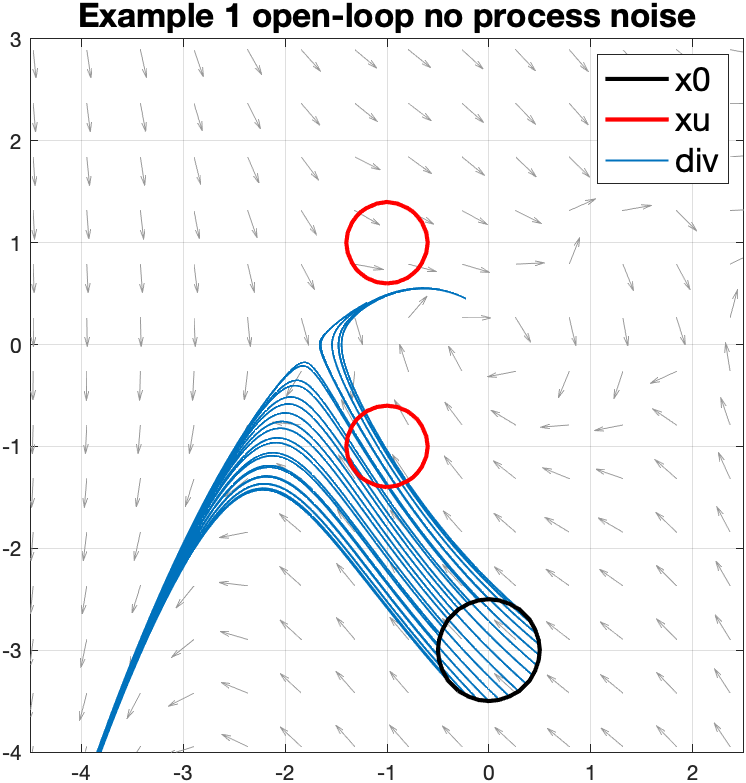
(a) open-loop

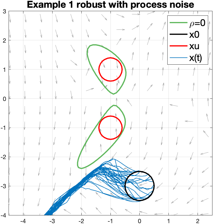
(b) robust closed-loop

Figure 1: Flow (21) simulations for Example 1

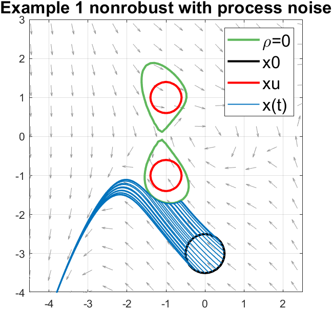
(a) no process noise

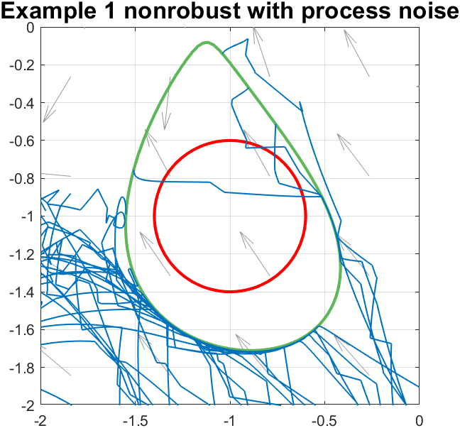
(b) with process noise

Figure 2: Safe controllers synthesized without process noise may be unsafe when process noise is applied

Results of the control design for Example 1 are shown in Fig. 1 and 2. In each figure, 30 trajectories (blue curves) start from within the initial set $\mathcal{X}_{0}$ (black circle). The unsafe set $\mathcal{X}_{u}$ is the pair of red disks, implemented as $h({{\mathbf{x}}})=-h_{1}({{\mathbf{x}}})h_{2}({{\mathbf{x}}})\geq 0$. Some of the open-loop trajectories in Fig. 1(a) enter the unsafe set $\mathcal{X}_{u}$ when starting in $\mathcal{X}_{0}$.

The prior knowledge of the system model is that $f$ is a two-dimensional cubic polynomial vector with $f(\mathbf{0})=\mathbf{0}$ and that $g$ is a two-dimensional constant vector, where the cubic polynomials in $f$ and the constant terms in $g$ are both unknown. 80 datapoints were collected and used to design a robustly safe controller under a sampling noise and a process noise bound of $\epsilon=\epsilon_{{\mathbf{w}}}=2$, yielding a polytope $\mathcal{P}_{2}$ from (14) with 22 dimensions ($\text{dim}({{\mathbf{f}}})=18,\ \text{dim}({{\mathbf{g}}})=2,\ \text{dim}({{\mathbf{w}}})=2$) and 324 faces (91 of the faces $\mathcal{P}_{2}$ are nonredundant [32]). Algorithm 1 was used to find $\rho,\psi\in\mathbb{R}[{{\mathbf{x}}}]_{\leq 4}$, yielding 99 Gram matrices of maximal size $\binom{6}{4}=15$ and the rational control law $u=\psi/\rho$. Fig. 1(b) plots trajectories associated with this safe control law, and also features the $\rho=0$ level set in green.

Fig. 2 highlights the importance of robustness in execution as well as in data-collection. The controller in Fig. 2 was computed with the same noisy observed data as in Fig. 1 but with $\epsilon_{{\mathbf{w}}}=0$. The left plot in Fig. 2(a) shows that the control is safe under noiseless trajectory execution. The right plot is zoomed into the lower red disk, and demonstrates that some controlled trajectories pass through the $\rho=0$ contour and enter $\mathcal{X}_{u}$ when process noise $\lVert{{\mathbf{w}}}\rVert_{\infty}\leq 2$ is applied in execution (trajectories are terminated when $u\geq 10^{4}$, which is caused by numerical issues near the $\rho=0$ contour).

To summarize this example, $\rho\geq 0$ is an invariant set for all consistent systems under online noise when the robust controller is applied. The level set $\rho=0$ will separates initial set $\mathcal{X}_{0}$ and the unsafe set $\mathcal{X}_{u}$. Uncontrolled (Fig. 1(a)) and non-robustly-safe (Fig. 2(b)) trajectories may enter $\mathcal{X}_{u}$.

Example 2.

Consider the Twist system [33] with:

$$f =\begin{bmatrix}-2.5x_{1}+x_{2}-0.5x_{3}+2x_{1}^{3}+2x_{3}^{3}\\ -x_{1}+1.5x_{2}+0.5x_{3}-2x_{2}^{3}-2x_{3}^{3}\\ 1.5x_{1}+2.5x_{2}-2x_{3}-2x_{1}^{3}-2x_{2}^{3}\end{bmatrix}, g =\begin{bmatrix}0\\ 0\\ 1\end{bmatrix}.$$ (22)

The initial and unsafe sets are the spheres:

$$\mathcal{X}_{0} =\{{{\mathbf{x}}}\mid 0.01-(x_{1}+0.5)^{2}-x_{2}^{2}-x_{3}^{2}\geq 0\},$$

$$\mathcal{X}_{u} =\{{{\mathbf{x}}}\mid 0.01-(x_{1}+0.1)^{2}-x_{2}^{2}-x_{3}^{2}\geq 0\}.$$

Results of Example 2 are are shown in Fig. 3. Trajectories start within the initial set $\mathcal{X}_{0}$ (black sphere), and some of the open-loop trajectories in Fig. 3(a) will enter the unsafe set $\mathcal{X}_{u}$ (red sphere). The prior knowledge of the system model is that $f$ is a three-dimensional cubic polynomial vector with $f(\mathbf{0})=\mathbf{0}$ and that $g$ is a three-dimensional constant vector. 80 datapoints were collected and used to design a robust safe controller under a sampling noise and a process noise bound of $\epsilon=\epsilon_{{\mathbf{w}}}=1$, yielding a polytope $\mathcal{P}_{2}$ with 63 dimensions ($\text{dim}({{\mathbf{f}}})=38,\ \text{dim}({{\mathbf{g}}})=3,\ \text{dim}({{\mathbf{w}}})=3$) and 304 faces (all of them are nonredundant). Using Algorithm 1 to find $\rho,\psi\in\mathbb{R}[{{\mathbf{x}}}]_{\leq 4}$ yields a rational control law $u=\psi/\rho$. Fig. 3(b) features the $\rho=0$ level set surface in green.

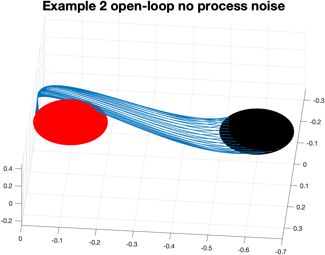
(a) open-loop

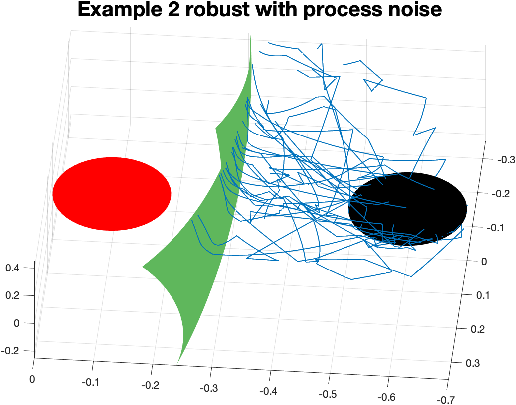
(b) robust closed-loop

Figure 3: Twist (22) simulations for Example 2.

5 Conclusion

This paper uses density functions to find provably safe controllers for systems whose data-observations and executions are both corrupted by $L_{\infty}$-bounded noise. The output of Algorithm 1 (if successful) is a rational controller $u$, along with a density certificate $\rho$ that guarantees robust safety of all trajectories starting in the initial set. Future work involves steering safe trajectories to a destination set (e.g. reach avoid, asymptotic stability), adding performance objectives, and extension to other noise and disturbance models (e.g. $L_{2}$ or semidefinite bounded signals).

References

- [1] S. Prajna and A. Jadbabaie, “Safety Verification of Hybrid Systems Using Barrier Certificates,” in HSCC, vol. 2993. Springer, 2004, pp. 477–492.
- [2] A. D. Ames, S. Coogan, M. Egerstedt, G. Notomista, K. Sreenath, and P. Tabuada, “Control Barrier Functions: Theory and Applications,” in 2019 18th European control conference (ECC). IEEE, 2019, pp. 3420–3431.
- [3] W. Xiao and C. Belta, “Control Barrier Functions for Systems with High Relative Degree,” in 2019 IEEE 58th conference on decision and control (CDC). IEEE, 2019, pp. 474–479.
- [4] A. D. Ames, J. W. Grizzle, and P. Tabuada, “Control Barrier Function Based Quadratic Programs with Application to Adaptive Cruise Control,” in 53rd IEEE Conference on Decision and Control. IEEE, 2014, pp. 6271–6278.
- [5] X. Xu, P. Tabuada, J. W. Grizzle, and A. D. Ames, “Robustness of Control Barrier Functions for Safety Critical Control,” IFAC-PapersOnLine, vol. 48, no. 27, pp. 54–61, 2015, analysis and Design of Hybrid Systems ADHS.
- [6] A. Majumdar, A. A. Ahmadi, and R. Tedrake, “Control Design along Trajectories with Sums of Squares Programming,” in 2013 IEEE International Conference on Robotics and Automation. IEEE, 2013, pp. 4054–4061.
- [7] A. Rantzer and S. Prajna, “On Analysis and Synthesis of Safe Control Laws,” in 42nd Allerton Conference on Communication, Control, and Computing. University of Illinois, 2004, pp. 1468–1476.
- [8] A. Rantzer, “A dual to Lyapunov’s stability theorem,” Systems & Control Letters, vol. 42, no. 3, pp. 161–168, 2001.
- [9] Y. Chen, M. Ahmadi, and A. D. Ames, “Optimal Safe Controller Synthesis: A Density Function Approach,” in 2020 American Control Conference (ACC), 2020, pp. 5407–5412.
- [10] S. Coogan, “Mixed Monotonicity for Reachability and Safety in Dynamical Systems,” in 2020 59th IEEE Conference on Decision and Control (CDC). IEEE, 2020, pp. 5074–5085.
- [11] S. Bansal, M. Chen, S. Herbert, and C. J. Tomlin, “Hamilton-Jacobi Reachability: A Brief Overview and Recent Advances,” in 2017 IEEE 56th Annual Conference on Decision and Control (CDC). IEEE, 2017, pp. 2242–2253.
- [12] L. Brunke, M. Greeff, A. W. Hall, Z. Yuan, S. Zhou, J. Panerati, and A. P. Schoellig, “Safe Learning in Robotics: From Learning-Based Control to Safe Reinforcement Learning,” Annual Review of Control, Robotics, and Autonomous Systems, vol. 5, pp. 411–444, 2022.
- [13] C. Folkestad, Y. Chen, A. D. Ames, and J. W. Burdick, “Data-Driven Safety-Critical Control: Synthesizing Control Barrier Functions with Koopman Operators,” IEEE Control Systems Letters, vol. 5, no. 6, pp. 2012–2017, 2020.
- [14] S. Formentin, K. Van Heusden, and A. Karimi, “A comparison of model-based and data-driven controller tuning,” International Journal of Adaptive Control and Signal Processing, vol. 28, no. 10, pp. 882–897, 2014.
- [15] T. Dai and M. Sznaier, “A Moments Based Approach to Designing MIMO Data Driven Controllers for Switched Systems,” in 2018 IEEE Conference on Decision and Control (CDC). IEEE, 2018, pp. 5652–5657.
- [16] T. Dai and M. Sznaier, “A Semi-Algebraic Optimization Approach to Data-Driven Control of Continuous-Time Nonlinear Systems,” IEEE Control Systems Letters, vol. 5, no. 2, pp. 487–492, 2020.
- [17] H. J. van Waarde, M. K. Camlibel, and M. Mesbahi, “From Noisy Data to Feedback Controllers: Nonconservative Design via a Matrix S-Lemma,” IEEE Trans. Automat. Contr., 2020.
- [18] T. Martin and F. Allgöwer, “Data-driven system analysis of nonlinear systems using polynomial approximation,” arXiv preprint arXiv:2108.11298, 2021.
- [19] J. Berberich, J. Köhler, M. A. Müller, and F. Allgöwer, “Data-Driven Model Predictive Control With Stability and Robustness Guarantees,” IEEE Trans. Automat. Contr., vol. 66, no. 4, pp. 1702–1717, 2021.
- [20] A. Bisoffi, C. De Persis, and P. Tesi, “Data-driven control via Petersen’s lemma,” Automatica, vol. 145, p. 110537, 2022.
- [21] J. Miller and M. Sznaier, “Data-Driven Gain Scheduling Control of Linear Parameter-Varying Systems using Quadratic Matrix Inequalities,” IEEE Control Systems Letters, 2022.
- [22] J. Miller, T. Dai, and M. Sznaier, “Data-Driven Superstabilizing Control of Error-in-Variables Discrete-Time Linear Systems,” in 2022 61st IEEE Conference on Decision and Control (CDC), 2022, pp. 4924–4929.
- [23] U. Rosolia and F. Borrelli, “Learning Model Predictive Control for Iterative Tasks. A Data-Driven Control Framework,” IEEE Transactions on Automatic Control, vol. 63, no. 7, pp. 1883–1896, 2018.
- [24] B. T. Lopez, J.-J. E. Slotine, and J. P. How, “Robust Adaptive Control Barrier Functions: An Adaptive and Data-Driven Approach to Safety,” IEEE Control Systems Letters, vol. 5, no. 3, pp. 1031–1036, 2021.
- [25] E. Daş and R. M. Murray, “Robust Safe Control Synthesis with Disturbance Observer-Based Control Barrier Functions,” in 2022 IEEE 61st Conference on Decision and Control (CDC). IEEE, 2022, pp. 5566–5573.
- [26] P. A. Parrilo, Structured Semidefinite Programs and Semialgebraic Geometry Methods in Robustness and Optimization. California Institute of Technology, 2000.
- [27] K. B. Petersen, M. S. Pedersen et al., “The Matrix Cookbook,” Technical University of Denmark, vol. 7, no. 15, p. 510, 2008.
- [28] M. Putinar, “Positive Polynomials on Compact Semi-algebraic Sets,” Indiana University Mathematics Journal, vol. 42, no. 3, pp. 969–984, 1993.
- [29] S. Boyd, S. P. Boyd, and L. Vandenberghe, Convex Optimization. Cambridge University Press, 2004.
- [30] J. Lofberg, “YALMIP : A toolbox for modeling and optimization in MATLAB,” in ICRA (IEEE Cat. No.04CH37508), 2004, pp. 284–289.
- [31] M. ApS, The MOSEK optimization toolbox for MATLAB manual. Version 9.2., 2020. [Online]. Available: https://docs.mosek.com/9.2/toolbox/index.html
- [32] R. Caron, J. McDonald, and C. Ponic, “A degenerate extreme point strategy for the classification of linear constraints as redundant or necessary,” Journal of Optimization Theory and Applications, vol. 62, no. 2, pp. 225–237, 1989.
- [33] J. Miller and M. Sznaier, “Bounding the Distance of Closest Approach to Unsafe Sets with Occupation Measures,” in 2022 IEEE 61st Conference on Decision and Control (CDC). IEEE, 2022, pp. 5008–5013.