Imitation and Transfer Learning for LQG Control

Abstract

In this paper we study an imitation and transfer learning setting for Linear Quadratic Gaussian (LQG) control, where (i) the system dynamics, noise statistics and cost function are unknown and expert data is provided (that is, sequences of optimal inputs and outputs) to learn the LQG controller, and (ii) multiple control tasks are performed for the same system but with different LQG costs. We show that the LQG controller can be learned from a set of expert trajectories of length $n(l+2)-1$, with $n$ and $l$ the dimension of the system state and output, respectively. Further, the controller can be decomposed as the product of an estimation matrix, which depends only on the system dynamics, and a control matrix, which depends on the LQG cost. This data-based separation principle allows us to transfer the estimation matrix across different LQG tasks, and to reduce the length of the expert trajectories needed to learn the LQG controller to $2n+m-1$ with $m$ the dimension of the inputs (for single-input systems with $l=2$, this yields approximately a $50\%$ reduction of the required expert data).

I Introduction

Imitation and transfer learning are popular techniques to learn optimal policies while reducing the amount of labeled data. In imitation learning, an agent is given access to samples of expert (optimal) behavior and seeks to learn a policy that mimics this behavior. In transfer learning, a model trained on one task is used as the starting point for a model on a second related task. The key idea is that certain features learned by the model on the first task can be used as a general-purpose set of features for the second task, allowing the model to learn the second task efficiently. While these techniques have proven useful in multiple learning scenarios, including image classification and natural language processing, their use and utility in control settings have mostly escaped scrutiny.

In this paper we investigate the use of imitation and transfer learning for Linear Quadratic Gaussian (LQG) control, which seeks a control policy for a stochastic linear system that minimizes the expected value of a quadratic function of the state and input [1]. We consider multiple control tasks, where the system dynamics are fixed but the quadratic cost function varies. We assume that the system dynamics, noise statistics, and cost functions are unknown, and that datasets are available containing optimal input and output trajectories for the different cost functions (source tasks). The questions that we answer include whether it is possible to learn the LQG controllers from expert data, the required size of the dataset, and whether the source datasets can be leveraged to learn the controller for a target task. We show that our data-based controller enjoys a separation property similar to the well-known separation principle [1], and that the lower-dimensional data-based estimation module can be transferred upon changes of the cost function to reduce the amount of expert data required for control design.

Related work. A number of approaches to direct and indirect data-driven control have recently been proposed. Most approaches focus on learning optimal policies from open-loop data for a fixed task and cost, e.g., see [2, 3, 4]. Differently from these works, this paper considers an imitation and transfer learning framework, where control policies are constructed by imitating expert demonstrations and transferring information across multiple, similar control tasks. Multi-task scenarios have received less attention, with [5, 6] and [7] being recent exceptions for system identification and control design, respectively. In [7], in particular, the notion of a common lower-dimensional representation among the tasks is used to reduce the amount of data required for control design across tasks. Similarly to [7], this paper also exploits a lower-dimensional representation for efficient transfer learning. However, differently from [7] and leveraging [8], this paper focuses on the LQG control problem and provides a precise, quantitative characterization of the lower-dimensional representation for multi-task LQG design from expert demonstrations, as well as tight bounds on the required data. This paper also differs from [9, 10], which study the sample complexity of learning LQG controllers in state-space form from open-loop data.

Contribution of the paper. The main contributions of this paper are as follows. First, we formalize an imitation and transfer learning setting for LQG control. We show that the LQG controller can be learned using an optimal input-output trajectory of length $n(l+2)-1$, where $n$ denotes the dimension of the system and $l$ the number of outputs. Further, we show that the proposed LQG controller is unique for the case of single-input systems, while it admits multiple representations for multi-input systems. Second, we prove the existence of a data-based separation principle since the data-based LQG controller can be written as the product of two matrices: the estimation matrix, which depends only on the system dynamics, and the controller matrix, which depends on the system dynamics and the quadratic cost function. Further, for the case of single-input systems, we show how the estimation matrix can be learned uniquely using the expert datasets (we also discuss and validate a procedure for the multi-input case). Third, we show how the data-based separation principle can be used for transfer learning because the estimation matrix remains invariant upon changes of the LQG cost function. By doing so, we show that an expert dataset of length $2n+m-1$ is sufficient to learn the LQG controller, thus confirming the benefits of transfer learning also for control design (for instance, for single input systems with $l=2$, our transfer learning technique reduces the amount of expert data by about $50\%$). As minor results, we show that the estimation matrix is of full row rank, thus suggesting the minimality of the internal representation, and that the system dimension can be learned using a single expert input-output trajectory of finite length.

II Problem formulation and preliminary results

Consider the discrete-time, linear, time-invariant system

$$x(t+1) =Ax(t)+Bu(t)+w(t),$$ (1)

$$y(t) =Cx(t)+v(t),\qquad t\geq 0,$$

where $x(t)\in{}^{n}$ denotes the state, $u(t)\in{}^{m}$ the control input, $y(t)\in{}^{l}$ the measured output, $w(t)$ the process noise, and $v(t)$ the measurement noise. We assume that the process and measurement noise sequences are independent at all times and satisfy $w(t)\sim\mathcal{N}(0,W)$ and $v(t)\sim\mathcal{N}(0,V)$, with $W\succeq 0$ and $V\succ 0$. Further, we assume that $(A,B)$ and $(A,W^{\frac{1}{2}})$ are controllable, and that $(A,C)$ is observable.

For the system (1), the Linear Quadratic Gaussian (LQG) control problem asks for an input that minimizes the cost

$$\lim_{T\rightarrow\infty}\mathbb{E}\left[\frac{1}{T}\Big{(}\sum_{t=0}^{T-1}x(t)^{\mathsf{T}}Qx(t)+u(t)^{\mathsf{T}}Ru(t)\Big{)}\right],$$ (2)

where $Q\succeq 0$, $R\succ 0$ are weight matrices and $T$ is the control horizon. We assume that $(A,Q^{\frac{1}{2}})$ is observable.

As a classic result [1], the optimal input that solves the LQG problem can be generated by a dynamic controller:

$$\hat{x}(t+1) =E\hat{x}(t)+Fu(t)+Gy(t+1),$$ (3)

$$u(t) =H\hat{x}(t),$$

where the controller matrices $E\in\mathbb{R}^{n\times n}$, $F\in\mathbb{R}^{n\times m}$, $G\in\mathbb{R}^{n\times l}$ and $H\in\mathbb{R}^{m\times n}$ can be obtained by combining the Kalman filter for (1) with the static controller that solves the Linear Quadratic Regulator (LQR) problem for (1) with weight matrices $Q$ and $R$ (separation principle). In this case, $\hat{x}(t)\in\mathbb{R}^{n}$ denotes the estimate of $x(t)$ generated by the Kalman filter and the controller matrices that satisfy

$$E =(I-L_{\text{f}}C)A, F=(I-L_{\text{f}}C)B,$$ (4)

$$G =L_{\text{f}}, H=K_{\text{LQR}},$$

where $K_{\text{LQR}}$ and $L_{\text{f}}$ are the LQR and Kalman gains, respectively. Although different choices are possible, we assume that the controller (3) uses the matrices (4) for simplicity and to further highlight the connections between our results and the classic separation-based solution to the LQG control problem. Additionally, we make the following technical assumption.

Assumption II.1

(Observability and controllability of the controller) Let $K_{\text{LQR},i}$ be the $i$-th row of the LQR gain ${K}_{\textup{LQR}}$. Then, the pair $(E,K_{\text{LQR},i})$ is observable for every $i\in\{1,\dots,m\}$, and the pair $(E,{L}_{\textup{f}})$ is controllable. $\square$

The optimal inputs generated by the dynamic controller (3) can also be obtained using a static gain and a finite window of past inputs and outputs [8]. In particular, the optimal LQG inputs $u^{*}$ satisfy the following relation:

$$u^{*}(t+n)={K}_{\textup{LQG}}\begin{bmatrix}U_{n}(t)\\ Y_{n}(t+1)\end{bmatrix},$$ (5)

where

$${K}_{\textup{LQG}} =H\begin{matrix}\begin{bmatrix}F_{u}+E^{n}F_{x}^{\dagger}(I-M_{u})&F_{y}-E^{n}F_{x}^{\dagger}M_{y}\end{bmatrix},\end{matrix}$$ (6)

and $U_{n}(t)$, $Y_{n}(t+1)$ are constructed as follows from $u^{*}$ and its corresponding output $y^{*}$ from the system (1),

$$U_{n}(t)=\begin{bmatrix}u^{*}(t)\\ \vdots\\ u^{*}(t+n-1)\end{bmatrix},Y_{n}(t+1)=\begin{bmatrix}y^{*}(t+1)\\ \vdots\\ y^{*}(t+n)\end{bmatrix},$$ (7)

and

$$M_{u} =\begin{bmatrix}0&\\ HF&&\\ \vdots&\ddots&&\\ HE^{n-2}F&\cdots&HF&0\end{bmatrix},F_{x}=\begin{bmatrix}H\\ HE\\ \vdots\\ HE^{n-1}\end{bmatrix},$$

$$F_{u} =\begin{bmatrix}E^{n-1}F&\cdots&F\end{bmatrix},$$

with $M_{y}$ and $F_{y}$ constructed in the same way as $M_{u}$ and $F_{u}$ by replacing $F$ by $G$. The expression (5) is convenient for learning purposes and it will be at the basis of our approach. The next technical result will be useful for our derivations (a proof can be found in the Appendix).

Lemma II.2

(Properties of input-output matrices) Let

$$H_{r,c}=\begin{bmatrix}U_{r}(t)&\cdots&U_{r}(t+c-1)\\ Y_{r}(t+1)&\cdots&Y_{r}(t+c)\end{bmatrix},$$ (8)

with $r\in\mathbb{N}_{\geq 0}$, $t\in\mathbb{N}_{\geq 0}$, and $U_{r}(t)$, $Y_{r}(t+1)$ as in (7). Then

$$\text{Rank}(H_{r,c})=\min\{mr+lr,c,n+lr\}.$$

The static LQG controller ${K}_{\textup{LQG}}$ can be computed using the static relation (5) and a sufficiently long, yet finite, optimal input-output trajectory. In fact, using optimal input and output sequences, the LQG gain (5) can be written as

$${K}_{\textup{LQG}}=\underbrace{\begin{bmatrix}u^{*}(t+n)&\cdots&u^{*}(t+n+c-1)\end{bmatrix}}_{\bar{U}_{c}}H_{n,c}^{\dagger},$$ (9)

with $c\geq n(l+1)$. Lemma II.2 implies that the data matrix $H_{n,c}$ in (9) is of full row rank for single-input systems. In this case, the gain ${K}_{\textup{LQG}}$ is unique and can be reconstructed exactly from data. On the other hand, $H_{n,c}$ in (9) loses rank for multi-input systems, in which case there exists multiple static LQG gains that satisfy the relation (5).

The design of the LQG compensator (3) or (5) is typically done using the system model (1), the noise statistics $W$ and $V$, and the cost matrices $Q$ and $R$. Instead, in this paper we are interested in solving the LQG problem in a data-driven setting and without identifying the system matrices. In particular, we consider an imitation and transfer learning scenario, where an expert provides a sequence of inputs $u^{*}$ minimizing the LQG cost (2) and the corresponding outputs $y^{*}$ of the system (1), for different choices of the weight matrices $Q$ and $R$. The question that we address is to quantify the sample complexity of learning the LQG controller. We show that, after sufficient training with different weight matrices, as little as ${2n+m-1}$ expert samples are sufficient to learn new LQG controllers.

To formalize the considered problem, let $D_{i}=\{u_{i}^{*},y_{i}^{*}\}_{t}^{t+T}$ be the sequence of expert (optimal) inputs solving the LQG problem from time $t$ up to time $t+T$ for the matrices $Q_{i}$ and $R_{i}$, and the corresponding outputs of the system (1). We assume that an expert provides optimal sequences for $N$ source LQG tasks, that is, $D_{1},\dots,D_{N}$, and one optimal sequence $D_{\text{target}}=\{u^{*}_{\text{target}},y^{*}_{\text{target}}\}_{t}^{t+\bar{T}}$ of length $\bar{T}$, with $(\bar{T}<T)$, for the target LQG task with matrices $Q_{\text{target}}$ and $R_{\text{target}}$. The objective is to learn the gain ${K}_{\textup{LQG}}$ for the target task using the data $D_{1},\dots,D_{N}$ and $D_{\text{target}}$. In particular, how large should $T$, $\bar{T}$ and $N$ be for this design to be feasible? We remark that the system dynamics and noise statistics are unknown and remain unchanged across all source and target tasks, and that the weight matrices associated with the source and target tasks are not known nor provided by the expert.

III Separation principle for data-driven LQG control and optimal internal representations

The separation principle states that the LQG controller can be designed by combining the solution to two separate simpler problems, namely, an optimal estimation problem and a deterministic optimal control problem with quadratic cost [1]. This insight is at the basis of the model-based design of the LQG controller. On the other hand, equation (5) shows that the LQG controller can assume a much simpler, static, form, but the expression lacks interpretability and does not hint to any separation of estimation and control. The next result bridges this gap by revealing a decomposition of ${K}_{\textup{LQG}}$ into independent controller and estimation matrices.

Theorem III.1

(Data-driven separation principle) Let ${K}_{\textup{LQG}}$ be as in (5). Then, using the notation in Equation (3),

$$\begin{aligned} {K}_{\textup{LQG}}=\underbrace{\begin{bmatrix}{K}_{\textup{LQR}}&I_{m}\end{bmatrix}}_{K}\underbrace{\begin{bmatrix}F_{u}-(a\otimes I_{n})\tilde{M}_{u}\!\!&\!\!F_{y}-(a\otimes I_{n})\tilde{M}_{y}\\ a\otimes I_{m}\!\!&\!\!0\end{bmatrix}}_{L_{\text{est}}},\end{aligned}$$

where

$$\tilde{M}_{u}=\begin{bmatrix}0\\ F&0\\ \vdots&\ddots&\ddots\\ E^{n-2}F&\cdots&F&0\end{bmatrix},\tilde{M}_{y}=\begin{bmatrix}0\\ G&0\\ \vdots&\ddots&\ddots\\ E^{n-2}G&\cdots&G&0\end{bmatrix},$$ (10)

and $a=\begin{bmatrix}a_{0}&\dots&a_{n-1}\end{bmatrix}$ such that

$$E^{n}=a_{0}I+a_{1}E+\cdots+a_{n-1}E^{n-1}.$$

Theorem III.1 shows how the LQG gain ${K}_{\textup{LQG}}$ can be decomposed as the product of ${L}_{\textup{est}}$, which depends only on the system matrices, and $K$, which depends on the LQR gain. Thus, Theorem III.1 shows that the separation principle also holds when representing the LQG controller as a function of the input and output sequences. While also interesting as a standalone result, Theorem III.1 becomes particularly useful in our imitation and transfer learning scenario. In fact, since ${L}_{\textup{est}}$ is independent of the LQR gain, it is also independent of the weight matrices $Q$ and $R$. Thus, ${L}_{\textup{est}}$ acts as an invariant component of the LQG controllers across different LQG tasks, which can reduce the amount of expert data required to construct LQG controllers (since ${L}_{\textup{est}}$ is common to all LQG tasks, only the matrix $K$ needs to be reconstructed for the LQG controller of the target task). We postpone the proof of Theorem III.1 to the Appendix.

The estimation matrix ${L}_{\textup{est}}$ is connected to the Kalman filter. To see this, notice that the optimal LQG inputs satisfy

$$u^{*}(t)={K}_{\textup{LQR}}\hat{x}(t),$$

where $\hat{x}(t)$ denotes the Kalman estimate of the state $x(t)$. Similarly, using Theorem III.1 and (5) we obtain

$$\begin{bmatrix}{K}_{\textup{LQR}}&I_{m}\end{bmatrix}\underbrace{{L}_{\textup{est}}\begin{bmatrix}U_{n}(t-n)\\ Y_{n}(t-n+1)\end{bmatrix}}_{z(t)}={K}_{\textup{LQR}}\hat{x}(t).$$

Thus, as the Kalman estimate provides an $n$-dimensional internal representation $\hat{x}(t)$ that can be used to generate optimal LQG inputs via the LQR gain in a model-based setting, the estimation matrix ${L}_{\textup{est}}$ provides an $(n+m)$-dimensional internal representation, $z(t)$, that can be used to generate optimal LQG inputs in a data-driven setting (given the matrix $K$). Yet, while the Kalman filter uses the whole history of inputs and outputs to generate an optimal internal representation (encoded in the state of the dynamic Kalman filter), the estimator ${L}_{\textup{est}}$ uses only a finite window of past inputs and outputs. Finally, as we show in the proof of Theorem III.5, the matrix ${L}_{\textup{est}}$ is of full row rank, thus suggesting that the internal representation $z(t)$ is of minimal dimension to compute LQG inputs from data.

Theorem III.1 provides a model-based expression of the control and estimation components that form the LQG controller. Next, we provide an expression of the estimation matrix ${L}_{\textup{est}}$ given data from a set of source LQG tasks. We start with the case of single-input systems and discuss the general case afterwards. We make the following technical assumption.

Assumption III.2

(Number and diversity of source tasks) Let $D_{1},\dots,D_{N}$ be the expert trajectories from the source LQG tasks with weight matrices $\{Q_{i},R_{i}\}_{i=1}^{N}$. Let ${K}_{\textup{LQG}}^{i}=K^{i}{L}_{\textup{est}}$ be the LQG gain of the $i$-th source task. Then,

$$\bigcap_{i=1}^{N}\operatorname{Ker}(K^{i})=\{0\}.$$

$\square$

We observe that the above condition is typically satisfied in practice when $N\geq n+m$ and for generic choices of the weight matrices, as it simply requires the LQR gains to be independent for different choices of the weight matrices.

Theorem III.3

(Learning ${L}_{\textup{est}}$ when $m=1$) Let $D_{1},\dots,D_{N}$ be the expert trajectories of length $T\geq n(l+2)-1$. Then,

$$\operatorname{Ker}({L}_{\textup{est}})=\;\bigcap_{i=1}^{N}\;\operatorname{Ker}(\bar{U}^{i}_{c_{s}}{H^{i^{\dagger}}_{n,c_{s}}}),$$ (11)

where $\bar{U}^{i}_{c_{s}}$ and $H^{i}_{n,c_{s}}$ are constructed as in (8) using the expert dataset $D_{i}$ with $c_{s}=T-n+1$.

Proof:

Let ${K}_{\textup{LQG}}^{i}$ be the LQG controller of the $i$-th task. From Theorem III.1 we have that ${K}_{\textup{LQG}}^{i}=K^{i}{L}_{\textup{est}}$. Then,

$$\operatorname{Ker}({K}_{\textup{LQG}}^{i}) =\operatorname{Ker}({L}_{\textup{est}})+{L}_{\textup{est}}^{\dagger}\left(\operatorname{Im}({L}_{\textup{est}})\cap\operatorname{Ker}(K^{i})\right)$$

$$=\operatorname{Ker}(\bar{U}^{i}_{c_{s}}H^{i^{\dagger}}_{n,c_{s}}),$$

where the last equality is due to Lemma II.2 (since $m=1$, $H^{i}_{n,c_{s}}$ is of full row rank and ${K}_{\textup{LQG}}^{i}=\bar{U}^{i}_{c_{s}}H^{i^{\dagger}}_{n,c_{s}}$. The claimed statement now follows from Assumption III.2. ∎

From Theorem III.3, the kernel of the estimation matrix ${L}_{\textup{est}}$ can be learned from a finite number of LQG datasets, with each dataset comprising optimal input and output trajectories of finite length. Hence, the estimation matrix ${L}_{\textup{est}}$ can also be learned up to multiplication by an invertible matrix using a basis of the orthogonal complement to $\operatorname{Ker}({L}_{\textup{est}})$. That is,

$${L}_{\textup{est}}=P\cdot\underbrace{\text{Basis}\left(\left(\bigcap_{i=1}^{N}\;\operatorname{Ker}(\bar{U}^{i}_{c_{s}}H^{i^{\dagger}}_{n,c_{s}})\right)^{\perp}\right)^{\mathsf{T}}}_{{\hat{L}}_{\textup{est}}},$$

for some invertible matrix $P$. Then, using Theorem III.1 and for any choice of the weight matrices $Q$ and $R$, the LQG controller for (1) can always be written as the product $KP^{-1}{\hat{L}}_{\textup{est}}$, where only the matrix $\hat{K}=KP^{-1}$ depends on the weight matrices $Q$ and $R$ and, from Theorem III.3, the estimation matrix ${\hat{L}}_{\textup{est}}$ can be learned given a sufficiently large and diverse dataset of expert trajectories. These observations imply that the controller for the target LQG task can be computed by simply learning the control matrix ${\hat{K}}_{\textup{target}}$ as a solution to the linear system

$${\bar{U}}^{\text{target}}_{c_{t}}={\hat{K}}_{\textup{target}}{\hat{L}}_{\textup{est}}H^{\text{target}}_{n,{c_{t}}},$$ (12)

where $\bar{U}_{c_{t}}^{\text{target}}$ and $H^{\text{target}}_{n,c_{t}}$ are constructed as in (8) from the target dataset ${D}_{\textup{target}}$, with $c_{t}=\bar{T}-n+1$. The next result quantifies the length of the expert trajectory $D_{\text{target}}$. We make the following assumption on the target dataset

Assumption III.4

(Persistency of excitation) For every value of $c_{t}$, the target dataset satisfies

$$\operatorname{Ker}({L}_{\textup{est}})\cap\operatorname{Im}(H^{\text{target}}_{n,c_{t}})=\{0\}.$$

$\square$

We remark that Assumption III.4 is generically satisfied since the entries of $H^{\text{target}}_{n,c_{t}}$ are driven by the system noise.

Theorem III.5

(Length of expert trajectory to learn the target LQG controller) Let $\bar{T}$ be the length of the expert trajectory in $D_{\text{target}}$. The LQG controller for the target task can be learned whenever $\bar{T}\geq 2n+m-1$.

Proof:

We first show that $\text{Rank}(F_{y}-(a\otimes I_{n})\tilde{M}_{y})=n$, which implies that ${L}_{\textup{est}}$ is of full row rank. With standard manipulation, the matrix $F_{y}-(a\otimes I_{n})\tilde{M}_{y}$ can be rewritten as

$$\underbrace{\begin{bmatrix}E^{n-1}&\cdots&I\end{bmatrix}}_{J}\underbrace{\begin{bmatrix}1\\ -a_{n-1}&1\\ \vdots&\ddots&\ddots\\ -a_{1}&\cdots&-a_{n-1}&1\end{bmatrix}}_{S}\underbrace{\begin{bmatrix}G\\ &\ddots&\\ &&G\end{bmatrix}}_{O}.$$

​​Notice that $S$ is invertible and that $\text{Rank}(JO)=\text{Rank}(F_{y})=n$ due to Assumption II.1. Then, $\text{Rank}(F_{y}-(a\otimes I_{n})\tilde{M}_{y})=\text{Rank}(JSO)=\text{Rank}(JO)=n$. Due to Assumption III.4 and Lemma II.2, the matrix $H^{\text{target}}_{n,{c_{t}}}$ has full column rank $n+m$ ($n+m\leq n(l+1)$) when $c_{t}=n+m$ (equivalently, $\bar{T}=2n+m-1$) and $\operatorname{Ker}({L}_{\textup{est}})\cap\operatorname{Im}(H^{\text{target}}_{n,c_{t}})=\{0\}$. Thus, ${L}_{\textup{est}}H^{\text{target}}_{n,{c_{t}}}$ is invertible, and finally ${K}_{\textup{target}}={\bar{U}}_{\textup{target}}({L}_{\textup{est}}{H}_{n,c_{t}}^{\text{target}})^{-1}$. ∎

Using (9), we notice that the LQG controller can be learned uniquely from a single trajectory of length $T\geq n(l+2)-1$ for the single-input case, since the data matrix in (9) becomes of full row rank. This bound reflects the complexity of learning the LQG controller in an imitation learning framework. On the other hand, leveraging the separation principle in Theorem III.1, the matrix ${\hat{L}}_{\textup{est}}$ can be learned from $N\geq n+1$ expert datasets and used to learn the LQG controller of any target task. By doing so, Theorem III.5 states that the expert trajectory of the target task needs only to be of length $2n$ for the single-input case. This reduced bound reflects the benefits of the imitation and transfer learning setting, where data from earlier tasks is used to solve future LQG tasks. For instance, when $m=1$ and $l=2$, the imitation and transfer approach requires about $50\%$ less expert data compared to the imitation approach alone.

Remark 1

(Learning the dimension of the system from data) The reconstruction of the LQG gain in (9) and of the estimation matrix in Theorem III.3 requires the knowledge of the dimension of the system to properly construct the required matrices. If unknown, the dimension of the system can be learned by solving the following minimization problem:

$$n=\min\{r\in\mathbb{N}\;:\;\text{Rank}(H_{r,r})=\text{Rank}(H_{r+1,r+1})\}.$$

This follows from Lemma II.2, since the rank of $H_{r,r}$ equals $n(l+1)$ when $r=n$ and the value of $l$ can be easily inferred from the expert data ($l$ equals the dimension of $y^{*}$). We note that this remark is also valid for multi-input systems. $\square$

Remark 2

(Learning ${L}_{\textup{est}}$ when $m>1$) Lemma II.2 implies that the data matrix in (9) is not full row rank when $m>1$ and that the LQG gain in (5) is not unique. Although the decomposition in Theorem III.1 still holds, the computation of ${L}_{\textup{est}}$ from data is more involved than the procedure presented in Theorem III.3. Here we discuss two different ways for this computation but, in the interest of space and clarity, we leave a detailed treatment for future research. First, let ${K}_{\textup{LQG}}^{i}$ be the LQG controller of the $i$-th source task. Then,

$${K}_{\textup{LQG}}^{i}=\bar{U}^{i}_{c_{s}}H^{i^{\dagger}}_{n,c_{s}}+X_{i}Z_{i}=K^{i}{L}_{\textup{est}}$$ (13)

for some matrix $X_{i}$, where $Z_{i}$ is a basis of the left null space of ${H^{i}_{n,c_{s}}}$. By stacking these expressions together we obtain

$$\begin{bmatrix}K^{1}\\ \vdots\\ K^{N}\end{bmatrix}{L}_{\textup{est}}=\begin{bmatrix}\bar{U}^{1}_{c_{s}}H^{i^{\dagger}}_{n,c_{s}}+X_{1}Z_{1}\\ \vdots\\ \bar{U}^{N}_{c_{s}}H^{N^{\dagger}}_{n,c_{s}}+X_{N}Z_{N}.\end{bmatrix}.$$ (14)

Since ${L}_{\textup{est}}$ has $n+m$ rows, where $n$ is obtained from Remark 1, the row space of every gain ${K}_{\textup{LQG}}^{i}$ must belong to the same $(n+m)$-dimensional subspace. Then, the matrix on the right hand side of (14) must have a left null space of dimension at least $mN-(n+m)$ for an appropriate choice of the matrices $X_{1},\dots,X_{N}$. This condition can be used to find the matrices $X_{1},\dots,X_{N}$ that satisfy (13) for a sufficiently large number $N$. Finally, similar to Theorem III.3,

$$\operatorname{Ker}({L}_{\textup{est}})\!=\;\bigcap_{i=1}^{N}\operatorname{Ker}(U^{i}_{n,c_{s}}H^{i^{\dagger}}_{n,c_{s}}+X_{i}Z_{i}).$$ (15)

Second, using the notation in Theorem III.3 and (12) and the fact that $\text{vec}(U^{i}_{c_{s}})=(H^{i^{\mathsf{T}}}_{n,c_{s}}\otimes K^{i})\text{vec}({L}_{\textup{est}})$, ${L}_{\textup{est}}$ can also be computed by solving the following bi-linear problem:

$$\min_{L,K^{1},\dots,K^{N}}\sum_{i=1}^{N}\|\text{vec}(\bar{U}^{i}_{c_{s}})-(H^{i^{\mathsf{T}}}_{n,c_{s}}\otimes K^{i})\text{vec}(L)\|.$$ (16)

The convergence properties of the two approaches above deserve a full discussion that is beyond the scope of this letter; in the next section we provide some numerical evidence. $\square$

IV Illustrative example

We use the following model of a batch reactor system that is open-loop unstable:

$$\begin{split}A&=\begin{bmatrix}[r]1.178&0.001&0.511&-0.403\\ -0.051&0.661&-0.011&0.061\\ 0.076&0.335&0.560&0.382\\ 0&0.335&0.089&0.849\end{bmatrix},B=\begin{bmatrix}[r]0.004\\ 0.467\\ 0.213\\ 0.213\end{bmatrix},\\ C&=\begin{bmatrix}[r]-0.44&-0.51&0.09&0.44\end{bmatrix},\end{split}$$ (17)

with process and measurement noise covariance $W=1.5I_{4}$ and $V=0.6$. The weight matrices of the target task are

$$Q_{\text{target}} =\begin{bmatrix}[r]6&1&1&-3\\ 1&1&0&-1\\ 1&0&3&0\\ -3&-1&0&2\\ \end{bmatrix},\text{ and }R_{\text{target}}=1.$$

We compare the model-based approach in Theorem III.1 with the data-driven approach in Theorem III.3. Using (6) we obtain

$${K}_{\textup{LQG}}^{\text{target}}\!=\!\begin{bmatrix}-0.01\!\!&\!\!0.16\!\!&\!\!-0.54\!\!&\!\!1.02\!\!&\!\!2.6\!\!&\!\!-13.34\!\!&\!\!21.25\!\!&\!\!-10.60\end{bmatrix}\!.$$

For our data-based approach, we have collected expert trajectories $D_{1},\dots,D_{N}$ of length $T=11$ from $N=5$ source tasks, with weighting matrices $Q_{i}=iI_{4}$ and $R_{i}=I_{2}$ respectively. Using Theorem III.3, we compute the estimation matrix ${\hat{L}}_{\textup{est}}$ as

$$\begin{bmatrix}[r]-0.01\!\!&\!0.09\!\!&\!-0.30\!\!&\!0.45\!\!&\!0.08\!\!&\!-0.42\!\!&\!0.65\!\!&\!-0.30\\ 0.02\!\!&\!-0.18\!\!&\!0.54\!\!&\!-0.61\!\!&\!0.07\!\!&\!-0.30\!\!&\!0.42\!\!&\!-0.19\\ 0.05\!\!&\!-0.34\!\!&\!0.57\!\!&\!0.56\!\!&\!0.12\!\!&\!-0.28\!\!&\!-0.10\!\!&\!0.38\\ -0.04\!\!&\!0.23\!\!&\!-0.32\!\!&\!-0.29\!\!&\!0.32\!\!&\!-0.60\!\!&\!-0.17\!\!&\!0.52\\ -0.05\!\!&\!0.17\!\!&\!0.03\!\!&\!-0.04\!\!&\!-0.43\!\!&\!0.26\!\!&\!0.54\!\!&\!0.65\end{bmatrix}$$

It can be verified that ${{K}_{\textup{LQG}}^{\text{target}}}^{\mathsf{T}}\in\operatorname{Im}({{\hat{L}}_{\textup{est}}}^{\mathsf{T}})$, that is, there exists a matrix ${\hat{K}}_{\textup{target}}$ such that ${K}_{\textup{LQG}}^{\text{target}}={\hat{K}}_{\textup{target}}{\hat{L}}_{\textup{est}}$. This verifies that the estimation matrix ${\hat{L}}_{\textup{est}}$ generates an internal representation from which the LQG inputs can be computed.

Consider now the same system (17) with two inputs, where the new input matrix and its corresponding cost matrix are:

$$B=\begin{bmatrix}[r]0.004&-0.087\\ 0.467&0.001\\ 0.213&-0.235\\ 0.213&-0.016\end{bmatrix},\text{ and }R_{\text{target}}=\begin{bmatrix}[r]1&0\\ 0&4\end{bmatrix}.$$

We follow the same steps as in the single input case to compute ${K}_{\textup{LQG}}^{\text{target}}$ using the model-based approach in (6), and then following the procedures in Remark (2), we compute ${\hat{L}}_{\textup{est}}$ using (15) and (16) respectively. In Fig. 1 we plot the error $\|{K}_{\textup{LQG}}^{\text{target}}(I-{\hat{L}}_{\textup{est}}^{\dagger}{\hat{L}}_{\textup{est}})\|$ for both approaches as the number of source tasks increases. The convergence of the error implies that ${\hat{L}}_{\textup{est}}$ obtained using the methods in Remark (2) becomes the correct estimation matrix for the target LQG controller.

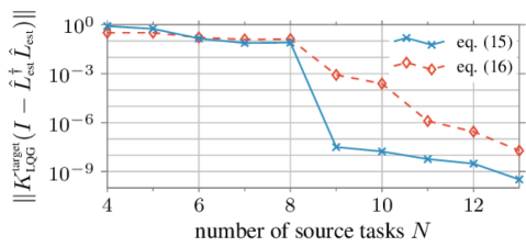
Figure 1: This figure shows the error $\|{K}_{\textup{LQG}}^{\text{target}}(I-{\hat{L}}_{\textup{est}}^{\dagger}{\hat{L}}_{\textup{est}})\|$ as a function of the number of source tasks. The error converges for (15) and (16) as the number of the source tasks increases, which implies that both approaches in Remark (2) reconstruct exactly the estimation matrix.

V Conclusion

In this paper we study an imitation and transfer learning setting for LQG control, where expert input-output trajectories are used to learn a data-based LQG controller. We show how the LQG controller can be computed from data, quantify the length of the expert trajectories needed to learn the controller, and show how the controller can be decomposed as the product of an estimation matrix, which depends only on the system dynamics, and a controller matrix, which depends also on the LQG cost. This separation principle allows us to reuse the estimation matrix across different LQG tasks, thus reducing the length of the required expert trajectories. Aspects of this research requiring additional investigation include a detailed treatment of the multi-input case, the study of transfer methods when the system dynamics also change, the extension to more general optimal control problems, and a proof of the minimality of the proposed internal representation.

-A Proof of Lemma II.2

Proof:

From (3) and (7) we have

$$U_{r}(t) =\underbrace{\begin{bmatrix}H\\ H\bar{E}\\ \vdots\\ H\bar{E}^{r-1}\end{bmatrix}}_{\bar{F}_{x}}\hat{x}(t)+\underbrace{\begin{bmatrix}0&0&\cdots&0\\ HG&0&\cdots&0\\ \vdots&\ddots&\ddots&\vdots\\ H\bar{E}^{r-2}G&\cdots&HG&0\end{bmatrix}}_{\bar{F}_{y}}Y_{r}(t+1),$$

where $\bar{E}=E+FH$. Then, we obtain

$$H_{r,c}=\underbrace{\begin{bmatrix}\bar{F}_{x}&\bar{F}_{y}\\ 0&I\end{bmatrix}}_{M}\underbrace{\begin{bmatrix}\hat{x}(t)&\!\!\cdots\!\!&\hat{x}(t+c-1)\\ Y_{r}(t+1)&\!\!\cdots\!\!&Y_{r}(t+c)\end{bmatrix}}_{N}.$$

Further, $\text{Rank}(H_{r,c})\leq\min\{\text{Rank}(M),\text{Rank}(N)\}$, and $\text{Rank}(H_{r,c})=\text{Rank}(M)$ whenever $N$ is of full row rank [11]. Notice that $\text{Rank}(M)\leq\min\{mr+lr,n+lr\}$, and $\text{Rank}(M)=n+lr$ if $mr\geq n$ and the pair $(\bar{E},H)$ is observable. To conclude, [12, Corollary 2] implies that $\text{Rank}(N)=\min\{n+lr,c\}$. ∎

-B Proof of Theorem III.1

We start with an alternative expression for ${K}_{\textup{LQG}}$.

Lemma .1

(Alternative expression for ${K}_{\textup{LQG}}$) Let $K_{\text{LQG},i}$ and $K_{\text{LQR},i}$ be the $i$-th row of ${K}_{\textup{LQG}}$ and ${K}_{\textup{LQR}}$, respectively, and define the matrices $P_{i}$ such that

$$P_{i}\underbrace{\begin{bmatrix}{K}_{\textup{LQR}}\\ {K}_{\textup{LQR}}E\\ \vdots\\ {K}_{\textup{LQR}}E^{n-1}\end{bmatrix}}_{F_{x}}=\underbrace{\begin{bmatrix}K_{\text{LQR},i}\\ K_{\text{LQR},i}E\\ \vdots\\ K_{\text{LQR},i}E^{n-1}\end{bmatrix}}_{F_{x}^{i}}.$$

for all $i\in\{1,\dots,m\}$. Then,

$$K_{\text{LQG},i}=K_{\text{LQR},i}\begin{bmatrix}F_{u}+E^{n}{F_{x}^{i}}^{\dagger}(P_{i}-M_{u}^{i})&F_{y}-E^{n}{F_{x}^{i}}^{\dagger}M_{y}^{i}\end{bmatrix},$$ (18)

where $F_{x}^{i}=P_{i}F_{x}$, $M_{u}^{i}=P_{i}M_{u}$, and $M_{y}^{i}=P_{i}M_{y}$.

Proof:

Using the compensator dynamics (3) we obtain

$$U_{n}(t) =F_{x}\hat{x}(t)+M_{u}U_{n}(t)+M_{y}Y_{n}(t+1),$$

and

$$\hat{x}(t+n) =E^{n}\hat{x}(t)+F_{u}U_{n}(t)+F_{y}Y_{n}(t+1).$$ (19)

Due to Assumption II.1, ${F}_{x}^{i}$ is invertible so that

$$\hat{x}(t)={F_{x}^{i}}^{\dagger}\left((P_{i}-M_{u}^{i})U_{n}(t)-M_{y}^{i}Y_{n}(t+1)\right),$$

for any $i\in\{1,\dots,m\}$ and, consequently,

$$\begin{split}\hat{x}(t+n)=E^{n}{F_{x}^{i}}^{\dagger}\big{(}(P_{i}-M_{u}^{i})U_{n}(t)&-M_{y}^{i}Y_{n}(t+1)\big{)}\\ +F_{u}U_{n}(t)+F_{y}Y_{n}(t+1).\end{split}$$ (20)

Notice that the gain $K_{\text{LQR},i}$ must satisfy, at all times,

$$K_{\text{LQR},i}\hat{x}(t+n)=K_{\text{LQG},i}\begin{bmatrix}U_{n}(t)\\ Y_{n}(t+1)\end{bmatrix}.$$

Substituting (20) into $\hat{x}(t+n)$ in (19) yields the result. ∎

We are now ready to prove Theorem III.1.

Proof of Theorem III.1:   Notice that (18) can be rewritten as

$$K_{\text{LQG},i}=\begin{bmatrix}K_{\text{LQR},i}&K_{\text{LQR},i}\end{bmatrix}\begin{bmatrix}F_{u}&F_{y}\\ E^{n}{F_{x}^{i}}^{\dagger}(I-M_{u}^{i})&-E^{n}{F_{x}^{i}}^{\dagger}M_{y}^{i}\end{bmatrix}.$$

Further, using the Cayley-Hamilton Theorem, we have

$$K_{\text{LQR},i}E^{n} =K_{\text{LQR},i}\left(a_{0}I_{n}+a_{1}E+\cdots+a_{n-1}E^{n-1}_{1}\right)$$

$$=\underbrace{\begin{bmatrix}a_{0}&a_{1}&\dots&a_{n-1}\end{bmatrix}}_{a}F_{x}^{i},$$

where $a_{0},\dots,a_{n-1}$ are the negative coefficients of the characteristic polynomial of $E$. Then, since $F_{x}^{i}$ is invertible (Assumption II.1), we have $K_{\text{LQR},i}E^{n}{F_{x}^{i}}^{\dagger}(P_{i}-M_{u}^{i})=a(P_{i}-M_{u}^{i})$ and $K_{\text{LQR},i}E^{n}{F_{x}^{i}}^{\dagger}M_{y}^{i}=aM_{y}^{i}$, and (18) becomes

$$K_{\text{LQG},i}=\begin{bmatrix}K_{\text{LQR},i}&1\end{bmatrix}\begin{bmatrix}F_{u}&F_{y}\\ a(P_{i}-M_{u}^{i})&-aM_{y}^{i}\end{bmatrix}.$$ (21)

Notice that

$$M_{u}^{i}\!=\!\underbrace{\begin{bmatrix}K_{\text{LQR},i}\!\!&\!\!\\ \!\!&\!\!\ddots\\ \!\!&\!\!\!\!&\!\!K_{\text{LQR},i}\end{bmatrix}}_{{K}_{\textup{diag}}}\tilde{M}_{u},\;M_{y}^{i}\!=\!\begin{bmatrix}K_{\text{LQR},i}\!\!&\!\!\\ \!\!&\!\!\ddots\\ \!\!&\!\!\!\!&\!\!K_{\text{LQR},i}\end{bmatrix}\tilde{M}_{y},$$

where $\tilde{M}_{u}$ and $\tilde{M}_{y}$ are defined in (10), and

$$a{K}_{\textup{diag}} =\begin{bmatrix}a_{0}K_{\text{LQR},i}&\cdots&a_{n-1}K_{\text{LQR},i}\\ \end{bmatrix}=K_{\text{LQR},i}\left(a\otimes I_{n}\right),$$

Thus, (21) becomes

$$K_{\text{LQG},i}=\begin{bmatrix}K_{\text{LQR},i}&1\end{bmatrix}\begin{bmatrix}F_{u}-(a\otimes I_{n})\tilde{M}_{u}&F_{y}-(a\otimes I_{n})\tilde{M}_{y}\\ aP_{i}&0\end{bmatrix}.$$

By using $\begin{bmatrix}(aP_{1})^{\mathsf{T}}&\cdots&(aP_{m})^{\mathsf{T}}\end{bmatrix}^{\mathsf{T}}=a\otimes I_{m},$ we obtain

$$\begin{bmatrix}K_{\text{LQG},1}\\ \vdots\\ K_{\text{LQG},m}\end{bmatrix}\!=\!\begin{bmatrix}{K}_{\textup{LQR}}\!\!&\!\!I_{m}\end{bmatrix}\begin{bmatrix}F_{u}-(a\otimes I_{n})\tilde{M}_{u}\!\!&\!\!F_{y}-(a\otimes I_{n})\tilde{M}_{y}\\ a\otimes I_{m}\!\!&\!\!0\end{bmatrix}.$$

This concludes the proof of Theorem III.1. $\blacksquare$

References

- [1] K. Zhou, J. C. Doyle, and K. Glover. Robust and Optimal Control. Prentice Hall, 1996.
- [2] B. Recht. A tour of reinforcement learning: The view from continuous control. Annual Review of Control, Robotics, and Autonomous Systems, 2:253–279, 2019.
- [3] K. Zhang, B. Hu, and T. Basar. Policy optimization for linear control with robustness guarantee: Implicit regularization and global convergence. In Learning for Dynamics and Control, volume 120 of Proceedings of Machine Learning Research, pages 179–190, Virtual, Jun. 2020. PMLR.
- [4] I. Markovsky and F. Dörfler. Behavioral systems theory in data-driven analysis, signal processing, and control. Annual Reviews in Control, 52:42–64, 2021.
- [5] L. Xin, L. Ye, G. Chiu, and S. Sundaram. Identifying the dynamics of a system by leveraging data from similar systems. In American Control Conference, pages 818–824, Atlanta, GA, USA, June 2022.
- [6] Y. Chen, A. M. Ospina, F. Pasqualetti, and E. Dall’Anese. Multi-task system identification of similar linear time-invariant dynamical systems. In IEEE Conf. on Decision and Control, Marina Bay Sands, Singapore, December 2023. Submitted. arXiv preprint arXiv:2301.01430.
- [7] T. T. Zhang, K. Kang, B. D. Lee, C. Tomlin, S. Levine, S. Tu, and N. Matni. Multi-task imitation learning for linear dynamical systems. arXiv preprint arXiv:2212.00186, 2022.
- [8] A. A. Al Makdah, V. Krishnan, V. Katewa, and F. Pasqualetti. Behavioral feedback for optimal LQG control. In IEEE Conf. on Decision and Control, Cancún, Mexico, December 2022.
- [9] S. Lale, K. Azizzadenesheli, B. Hassibi, and A. Anandkumar. Logarithmic regret bound in partially observable linear dynamical systems. In Advances in Neural Information Processing Systems, volume 33, pages 20876–20888, Virtual, Dec. 2020. Curran Associates, Inc.
- [10] Y. Zheng, L. Furieri, M. Kamgarpour, and N. Li. Sample complexity of linear quadratic gaussian (LQG) control for output feedback systems. In Learning for Dynamics and Control, volume 144 of Proceedings of Machine Learning Research, pages 559–570, Virtual, Jun. 2021. PMLR.
- [11] R. A. Horn and C. R. Johnson. Matrix Analysis. Cambridge University Press, 1985.
- [12] J. C. Willems, P. Rapisarda, I. Markovsky, and B. L. M. De Moor. A note on persistency of excitation. Systems & Control Letters, 54(4):325–329, 2005.