Physics-Informed Neural Networks
for Time-Domain Simulations:
Accuracy, Computational Cost, and Flexibility

Abstract

The simulation of power system dynamics poses a computationally expensive task. Considering the growing uncertainty of generation and demand patterns, thousands of scenarios need to be continuously assessed to ensure the safety of power systems. Physics-Informed Neural Networks (PINNs) have recently emerged as a promising solution for drastically accelerating computations of non-linear dynamical systems. This work investigates the applicability of these methods for power system dynamics, focusing on the dynamic response to load disturbances. Comparing the prediction of PINNs to the solution of conventional solvers, we find that PINNs can be 10 to 1’000 times faster than conventional solvers. At the same time, we find them to be sufficiently accurate and numerically stable even for large time steps. To facilitate a deeper understanding, this paper also present a new regularisation of Neural Network (NN) training by introducing a gradient-based term in the loss function. The resulting NNs, which we call dtNNs, help us deliver a comprehensive analysis about the strengths and weaknesses of the NN based approaches, how incorporating knowledge of the underlying physics affects NN performance, and how this compares with conventional solvers for power system dynamics.

(0.0cm,2.5cm) Manuscript published in journal
DOI: https://doi.org/10.1016/j.epsr.2023.109748
Received 16 March 2023, Revised 7 July 2023, Accepted 3 August 2023
© 2023. This manuscript version is made available under the CC-BY-NC-ND 4.0 license https://creativecommons.org/licenses/by-nc-nd/4.0

1 Introduction

Time-domain simulations form the backbone in many power system analyses such as transient or voltage stability analyses. However, even the simplest set of governing Differential-Algebraic Equations (DAEs) which can describe the system dynamics sufficiently accurate, can impose a significant computational burden during the analysis. Ways to reduce this computational cost while maintaining a sufficiently high level of accuracy is of paramount importance across all applications in the power systems industry.

Since, generally speaking, there is no closed form analytical solution for DAEs [1], we revert to numerical methods to approximate the dynamic response. Refs. [2, 3] provide a good overview on general solution approaches and the modelling in the power system context, and [4, 5, 6] summarise important developments, mostly relying on model simplification, decompositions, pre-computing partial solutions, and parallelisations.

A new avenue to solve ordinary and partial differential equations emerged recently through so-called Scientific Machine Learning (SciML)– a field, which combines scientific computing with Machine Learning (ML). SciML has been receiving a lot of attention due to the significant potential speed-ups it can achieve for computationally expensive problems, such as the solution of differential equations. More specifically, the authors in [7], already 25 years ago, introduced the idea of using artificial Neural Networks (NNs) to approximate such solutions. The idea is that NNs learn from a set of training data to interpolate the solution for data points that lie between the training data with high accuracy. Ref. [8] has revived this effort, now named Physics-Informed Neural Networks (PINNs), which has developed into a growing field within SciML as [9] reviews. The key idea of PINNs is to directly incorporate the domain knowledge into the learning process. We do so by evaluating if the NN output satisfies the set of DAEs during training. If it does not, the parameters of the NN are adjusted in the next training iteration until the NN output satisfies the DAEs. This approach reduces the need for large training datasets and hence the associated costs for simulating them. Ref. [10] introduced PINNs in the field of power systems.

Our ultimate goal is to develop PINNs as a solution tool for time-domain simulations in power systems. This paper takes a first step, and identifies the strengths and weaknesses of such a method in comparison with existing solution methods with respect to the application specific requirements on the solution method. Stott elaborated nearly half a century ago that, among others, sufficient accuracy, numerical stability, and flexibility were important characteristics that need to be weighed against the solution speed [2]. In an ideal world, we are looking for tools that are highly accurate, numerically stable, and flexible, and at the same time very fast. Several approaches have been proposed to deal with this trade-off, aiming at being faster (at least during run-time) while maintaining accuracy, numerical stability, and flexibility to the extent possible. Some of the promising ones are based on pre-computing parts of the solution of DAEs. For example, Semi-Analytical Solution (SAS)-methods adopt this approach [11, 12, 13]. We can push this idea of pre-computing the solution even further: PINNs, and NNs in general, pre-compute – learn – the entire solution, hence, the computation at run-time is extremely fast. Related works in [14, 15, 16] introduce alternative NN architectures and problem setups, primarily driven by considerations on the achieved accuracy. In contrast, our focus lies on assessing PINNs from a perspective of a numerical solution method in which accuracy has to be weighed against other numerical characteristics namely speed, numerical stability and flexibility. The contributions of this work are the following:

1. We apply Physics-Informed Neural Networks (PINNs)to multi-machine systems and show that PINNs can be 10 to 1’000 times faster than conventional methods for time-domain simulations, while achieving sufficient accuracy.

2. We demonstrate that the trade-off between speed and accuracy for PINNs, and NNs in general, does not directly relate to power system size but rather to the complexity of the dynamics. Hence, NNs can solve larger systems equally fast as small ones, if the complexity of the dynamics is comparable. This is contrary to conventional methods, where the solution time is closely linked to the system size.

3. We examine further numerical properties of NNs for solving DAEs. Besides speed, one of their key benefits is that NNs do not suffer from numerical instability as they solve without any iterative procedure. We also discuss the challenges of flexibility in different parameter settings and we outline concrete directions for future work to resolve them.

4. Having shown that NNs do have significant benefits and desirable properties, we carry out a comprehensive analysis on the performance and training of NNs and PINNs that can be helpful for future applications. In this context, we introduce dtNNs, a regularised form of NNs. dtNNs are an intermediate methodological step between NNs and PINNs as they are regularised by the time derivatives at the training data points.

Section 2 describes the construction of a NN-based approximation for DAEs and how to incorporate physical knowledge in dtNNs and PINNs. Section 3 presents the case study and the training setup. Section 4 shows the results, on which basis we discuss the route forward in Section 5. Section 6 concludes.

2 Methodology

This section lays out how we train a NN that shall be used in time-domain simulations, how the physical equations can be incorporated transforming the NN to a dtNN and a PINN, and how the resulting approximation is assessed.

2.1 Approximating the solution to a dynamical system

A dynamical system is characterised by its temporal evolution being dependent on the system’s state variables $\bm{x}$, the algebraic variables $\bm{y}$ and the control inputs $\bm{u}$:

$$\frac{d}{dt}\bm{x} =\bm{f}_{\text{DAE}}\left(\bm{x}(t),\bm{y}(t),\bm{u}\right)$$ (1a)

$$\bm{0} =\bm{g}_{\text{DAE}}\left(\bm{x}(t),\bm{y}(t),\bm{u}\right).$$ (1b)

For clarity and ease of implementation, we express 1a and 1b as

$$\bm{M}\frac{d}{dt}\bm{x} =\bm{f}(\bm{x}(t),\bm{u}).$$ (2)

by incorporating $\bm{y}$ into $\bm{x}$ and adding $\bm{M}$, which is a diagonal matrix to distinguish if a state $x_{i}$ is differential $(M_{ii}\neq 0)$ or algebraic $(M_{ii}=0)$. We will use a NN to define an explicit function $\hat{\bm{x}}(t)$ that shall approximate the solution $\bm{x}(t)$ for all $t\in[t_{0},t^{\max}]$, i.e., for the entire trajectory, starting from the initial condition $\bm{x}(t_{0})=\bm{x}_{0}$.

2.2 Neural network as function approximator

We use a standard feed-forward NN with $K$ hidden layers that implements a sequence of linear combinations and non-linear activation functions $\sigma(\cdot)$. In theory, a NN with a single hidden layer already constitutes a universal function approximator [17] if it is wide enough, i.e., the hidden layer consists of enough neurons $N_{K}$. In practice, restrictions on the width and the process of determining the NN’s parameters might limit this universality as [18] elaborates. Still, a multi-layer NN in the form of (3) provides us with a powerful function approximator:

$$[t,\bm{x}_{0}^{\top},\bm{u}^{\top}]^{\top} =\bm{z}_{0}$$ (3a)

$$\bm{z}_{k+1} =\sigma{(\bm{W}_{k+1}\bm{z}_{k}+\bm{b}_{k+1})} \quad\forall k=0,1,...,K-1$$ (3b)

$$\hat{\bm{x}} =\bm{W}_{K+1}\bm{z}_{K}+\bm{b}_{K+1}.$$ (3c)

The NN output $\hat{\bm{x}}$ is the system state at the prediction time $t$. The input $\bm{z}_{0}$ is composed of the prediction time $t$, the initial condition $\bm{x}_{0}$ and the control input $\bm{u}$. The weight matrices $\bm{W}_{k}$ and bias vectors $\bm{b}_{i}$ form the adjustable parameters $\bm{\theta}$ of the NN.

For the training process, we compile a training dataset $\mathcal{D}_{\text{train}}$, that maps $\bm{z}_{0}\mapsto\bm{x}$ for a chosen input domain $\mathcal{Z}$ and contains $N=|\mathcal{D}_{\text{train}}|$ points. For our purposes, the input domain is a discrete set of the prediction time, e.g. from $0\text{\,}\mathrm{s}$ until $10\text{\,}\mathrm{s}$ with a step size of $0.2\text{\,}\mathrm{s}$, and a set of different initial conditions and control inputs, e.g. different power disturbances. The output domain is the rotor angle and frequency at each of the prediction time steps and for each of the studied disturbances.

$$\mathcal{D}_{\text{train}}:\bm{z}_{0}\mapsto\bm{x}\qquad\bm{z}_{0}\in\mathcal{Z}.$$ (4)

During training we adjust the NN’s parameters $\bm{\theta}$ with an iterative gradient-based optimisation algorithm to minimise the so-called loss $\mathcal{L}$ for $\mathcal{D}_{train}$

$$\min_{\bm{\theta}}\quad \mathcal{L}(\mathcal{D}_{\text{train}})$$ (5a)

s.t. $$\eqref{eq:NN_input}-\eqref{eq:NN_output}.$$ (5b)

We do not aim for optimality of 5 – this would lead to over-fitting – but rather search for parameters $\bm{\theta}$ (i.e., values of the weights and biases) and hyper-parameters (e.g., number of layers $K$ and neurons per layer $N_{K}$) that yield a low generalisation error $\mathcal{L}(\mathcal{D}_{\text{test}})$ which we assess on a separate test dataset $\mathcal{D}_{\text{test}}$. During training we use a validation dataset $\mathcal{D}_{\text{validation}}$ to obtain an estimate of the generalisation error, so that the final evaluation with $\mathcal{D}_{\text{test}}$ remains unbiased. It is important, that all three datasets stem from the same sampling procedure and input domain $\mathcal{Z}$.

2.3 Loss function and regularisation: NNs, dtNNs, and PINNs

2.3.1 Loss Function for Neural Networks

The simplest loss function for such a problem is to define the loss as the mismatch between the NN prediction $\hat{\bm{x}}$ and the ground truth or target $\bm{x}$, and measure it using the L2-norm. To account for different orders of magnitude (for example, the voltage angles in radians are often much larger than frequency deviations expressed in $\mathrm{p.u.}$) and levels of variations of the individual states $\bm{x}$, we first apply a scaling factor $\xi_{x,i}$ to the error computed per state $i$. A physics-agnostic choice of $\xi_{x,i}$ could be to use the state’s standard deviation in the training dataset; for more details please see Section 3.2. We then apply the squared L2-norm for each data point $j$ and take the average across the dataset $\mathcal{D}_{\text{}}$ to obtain the loss $\mathcal{L}_{x}$

$$\mathcal{L}_{x}(\mathcal{D}_{\text{}}) =\frac{1}{|\mathcal{D}_{\text{}}|}\sum_{j=1}^{|\mathcal{D}_{\text{}}|}\left\lVert\left(\frac{\hat{x}_{i}^{j}-x_{i}^{j}}{\xi_{x,i}{}}\right)\right\rVert_{2}^{2}.$$ (6)

2.3.2 dtNNs

As an intermediate step between standard NNs and PINNs, in this subsection we introduce a new regularisation term to loss function (6). We do so to avoid the previously mentioned over-fitting and improve the generalisation performance of the NNs. To the best of our knowledge, this paper is the first to introduce a regularisation term based on the update function $\bm{f}$($\bm{x}$) from (2). Using the tool of Automatic Differentiation (AD) [19], we can compute the derivative of the NN, i.e., the time derivative of the approximated trajectory, $\frac{d}{dt}\hat{\bm{x}}{}$ and compute a loss analogous to (6) (with a scaling factor $\xi_{dt,i}$):

$$\mathcal{L}_{dt}(\mathcal{D}_{\text{}}) =\frac{1}{|\mathcal{D}_{\text{}}|}\sum_{j=1}^{|\mathcal{D}_{\text{}}|}\left\lVert\left(\frac{\frac{d}{dt}\hat{x}_{i}^{j}-\frac{d}{dt}x_{i}^{j}}{\xi_{dt,i}{}}\right)\right\rVert_{2}^{2}$$ (7)

2.3.3 PINNs

As [7, 8] introduced generally, and [10] for power systems, we can also regularise such a NN by comparing the derivative of the NN $\frac{d}{dt}\hat{\bm{x}}{}$ with the update function evaluated based on the estimated state $\bm{f}$($\hat{\bm{x}}$):

$$\mathcal{L}_{f}(\mathcal{D}_{f}) =\frac{1}{|\mathcal{D}_{f}|}\sum_{j=1}^{|\mathcal{D}_{f}|}\left\lVert\left(\frac{M_{ii}\frac{d}{dt}\hat{x}_{i}^{j}-f_{i}(\hat{\bm{x}}^{j})}{\xi_{f,i}{}}\right)\right\rVert_{2}^{2}$$ (8)

This physics-loss does not require the ground truth state $\bm{x}$ or its derivative. Quite the contrary, this loss can be queried for any desired point without requiring any form of simulation. We therefore can evaluate a dataset $\mathcal{D}_{f}$ of randomly sampled or ordered collocation points that map to 0

$$\mathcal{D}_{f}:\bm{z}_{0}\mapsto\bm{0}\qquad\bm{z}_{0}\in\mathcal{Z}.$$ (9)

to essentially assess how well the NN approximation follows the physics - any point where this physics loss equals zero is in line with the governing physics of (2). However, (9) defines a mapping that is not bijective, hence, $\mathcal{L}_{f}(\mathcal{D}_{f})=0$ does not imply that the desired trajectory is perfectly matched, only that a trajectory complying with (2) is matched. As an example, an exact prediction of the steady state of the system will yield $\mathcal{L}_{f}(\mathcal{D}_{f})=0$ even though the target trajectory in $\mathcal{D}_{\text{train}}$ is different.

2.3.4 Combined loss function during training

To obtain a single objective or loss value for the training problem (5), we weigh the three terms as follows:

$$\mathcal{L} =\mathcal{L}_{x}+\lambda_{dt}\mathcal{L}_{dt}+\lambda_{f}\mathcal{L}_{f},$$ (10)

where $\lambda_{dt}$ and $\lambda_{f}$ are hyper-parameters of the problem. Subsequently, we refer to a NN trained with $\lambda_{dt}{}=0,\lambda_{f}{}=0$ as vanilla NN, with $\lambda_{dt}{}\neq 0$, $\lambda_{f}{}=0$ as dtNN, and with $\lambda_{dt}{}\neq 0,\lambda_{f}{}\neq 0$ as PINN.

2.4 Accuracy metrics

To compare across the different methods and setups, we monitor the loss $\mathcal{L}_{x}$ in (6) as the comparison metric throughout the training and evaluation process and as an accuracy metric for the performance assessment. To get a more detailed picture, we also consider the loss value of single points, i.e., before calculating the mean in 6. However, the loss is dependent on the chosen values for $\xi_{x,i}{}$ and does not provide an easily interpretable meaning. Therefore, we use the maximum absolute error

$$\max AE_{\mathcal{S}} =\max_{i\in\mathcal{S},j\in\mathcal{D}_{\text{test}}}\left(\left|\hat{x}_{i}^{j}-x_{i}^{j}\right|\right)$$ (11)

as an additional metric for assessment purposes, i.e., based on $\mathcal{D}_{\text{test}}$, but not during training. Whereas a state-by-state metric would capture most details, we opt to compute the maximum absolute error across meaningful groups of states $i\in\mathcal{S}$ that are of the same units and magnitudes. This aligns with the engineering perspective on the desired accuracy of a method.

3 Case study

This section introduces the test cases and the details of the NN training.

3.1 Power system - Kundur 11-bus and IEEE 39-bus system

As a study setup, we investigate the dynamic response of a power system to a load disturbance. We use a second order model to represent each of the generators in the system. The update equation 2 formulates for generator buses as

$$\begin{bmatrix}1&0\\ 0&2H_{i}\omega_{0}\end{bmatrix}\frac{d}{dt}\begin{bmatrix}\delta_{i}\\ \Delta\omega_{i}\end{bmatrix} =\begin{bmatrix}\Delta\omega_{i}\\ P_{mech,i}-D_{i}\Delta\omega_{i}+P_{e,i}\end{bmatrix}$$ (12)

and for load buses as

$$\begin{bmatrix}d_{i}\omega_{0}\end{bmatrix}\frac{d}{dt}\begin{bmatrix}\delta_{i}\end{bmatrix} =\begin{bmatrix}P_{mech,i}+P_{e,i}\end{bmatrix}$$ (13)

where $P_{mech,i}=P_{set,i}+P_{dist,i}$ at bus $i$, with $P_{set,i}$ representing the power setpoint and $P_{dist,i}$ the disturbance . The states $\bm{x}$ are the bus voltage angle $\delta_{i}$ and the frequency deviation $\Delta\omega_{i}$ for generator buses, and the bus voltage angle $\delta_{i}$ for the load buses. The buses are linked through the active power flows in the network defined by the admittance matrix $\bar{\bm{Y}}_{bus}$ and the vector of complex voltages $\bar{\bm{V}}=\bm{V}_{m}e^{j\bm{\delta}}$, where the vector $\bm{V}_{m}$ collects the voltage magnitudes and $\bm{\delta}$ the bus voltage angles:

$$\bm{P}_{e} =\Re\left(\bar{\bm{V}}(\bar{\bm{Y}}_{bus}\bar{\bm{V}})^{*}\right).$$ (14)

The $*$ indicates the complex conjugate and $P_{e,i}$ corresponds to the $i$-th entry of vector $\bm{P}_{e}$, i.e., the active power balance at bus $i$. In Section 4, we demonstrate the methodology on the Kundur 2-area system (11 buses, 4 generators) and the IEEE 39-bus test system (39 buses, 10 generators). For both systems we are using the base power of $100\text{\,}\mathrm{M}\mathrm{V}\mathrm{A}$ and $\omega_{0}=$60\text{\,}\mathrm{Hz}$$. The network parameters and set-points stem from the case description of Kundur [21, p. 813] and the IEEE 39-bus test case in Matpower [22]. The values for the inertia of the generators $H_{i}$ are [6.5, 6.5, 6.175, 6.175] $\mathrm{p.u.}$ for the 11-bus case and [500.0, 30.3, 35.8, 38.6, 26.0, 34.8, 26.4, 24.3, 34.5, 42.0] $\mathrm{p.u.}$ for the 39-bus case. The damping factor was set to $D_{i}=0.05\frac{\omega_{0}}{P_{set,i}}$ in both cases and for the loads to $d_{i}=1.0\frac{P_{set,i}}{\omega_{0}}$ and $d_{i}=0.2\frac{P_{set,i}}{\omega_{0}}$ respectively.

3.2 NN training implementation

The entire workflow is implemented in Python 3.8 and available under [23]. When we use the conventional numerical approaches to carry out the time-domain simulations for this system, the dynamical system is simulated using the Assimulo package [24] which implements various solution methods for systems of DAEs. The training process utilises PyTorch [25] for the learning process and WandB [26] for monitoring and processing the workflow. The implementation builds on [27] for the steps of the workflow.

All datasets comprise the simulated response of the system over a period of $20\text{\,}\mathrm{s}$ to a disturbance. The tested disturbance is the step response to an instantaneous loss of load $|P_{dist,i}|$ at bus $i$ with a magnitude between $0\text{\,}\mathrm{p.u.}$ and $10\text{\,}\mathrm{p.u.}$, where $i=7$ for the 11-bus system and $i=20$ for the 39-bus system. We record these data in increments of $\Delta t$ and $\Delta P$. The test dataset $\mathcal{D}_{\text{test}}$ which shall serve as a ground truth uses $\Delta t=$0.05\text{\,}\mathrm{s}$$ and $\Delta P=$0.05\text{\,}\mathrm{p.u.}$$, resulting in $|\mathcal{D}_{\text{test}}|=401\times 201=80601$ points. This large size of $\mathcal{D}_{\text{test}}$ is chosen as it densely covers the input domain, hence, we obtain a reliable estimate of the maximum absolute error 11. For the training datasets $\mathcal{D}_{\text{train}}$ used in Section 4.2 we create datasets with $\Delta t\in[$0.2$,$1.0$,$2.0$]$\mathrm{s}$$ and $\Delta P\in[$0.2$,$1.0$,$2.0$]$\mathrm{p.u.}$$. The validation datasets $\mathcal{D}_{\text{validation}}$ for those scenarios are offset by $\frac{\Delta t}{2}$ and $\frac{\Delta P}{2}$.

For the scalings $\xi_{x,i}$ in (6), we calculate the average standard deviation $\sigma$ across all voltage angle differences $\delta_{ij}$ and all frequency deviations $\Delta\omega_{i}$, here the relevant groups of states $\mathcal{S}$:

$$\xi_{x,i}{} =\frac{1}{|\mathcal{S}|}\sum_{i\in\mathcal{S}}\sigma(x_{i}(\mathcal{D}_{\text{}}))$$ (15)

Thereby, we aim for equal levels of error within all $\delta_{ij}$ and $\Delta\omega_{i}$ states and account for the difference in magnitude between them. $\xi_{dt,i}$ and $\xi_{f,i}$ are all set to 1.0 to avoid adding further hyperparameters, more elaborate choices based on system analysis or the database are conceivable. During training and testing $\xi_{x,i}$ is based on $\mathcal{D}_{\text{train}}$ and $\mathcal{D}_{\text{test}}$ respectively.

The regularisation weights $\lambda_{dt}$ and $\lambda_{f}$ are hyperparameters. For the latter, we incorporate a fade-in dependent on the current epoch $E$ :

$$\lambda_{f}{}(E)=\min{\left(\lambda_{f,\max}{};\lambda_{f,0}{}\;10^{E/E^{\prime}}\right)},$$ (16)

where $\lambda_{f,\max}$ is the maximum and $\lambda_{f,0}$ the initial regularisation weight and $E^{\prime}$ determines the “speed” of the fade-in. The fade-in causes that $\mathcal{L}_{x}$ and $\mathcal{L}_{dt}$ are first minimised and then $\mathcal{L}_{f}$ helps for “fine-tuning” and better generalisation. We apply the limited-memory Broyden-Fletcher-Goldfarb-Shanno (L-BFGS) algorithm implemented in PyTorch in the training process, a standard optimiser for PINNs as [28] reviews. The set of hyperparameters comprises $K$, $N_{K}$, $\lambda_{dt}$, $\lambda_{f,\max}$, $\lambda_{f,0}$ $E^{\prime}$, and additional L-BFGS parameters. Table 1 reports the used hyperparameters for the scenarios (letters A-E) in Section 4.2, Section 4.1 is based on scenario E for vanilla NNs.

Table 1: Overview of the tuning range and the selected values of the involved hyperparameters.

		vanilla NN		dtNN		PINN
Hyper-parameter	Tuning range	A-D	E	A-D	E	A-D	E
Number of layers $K$	[2, 3, 4, 5]	5	5	5	5	5	5
Nodes per layer $N_{K}$	[16, 32, 64, 128]	32	32	32	32	32	32
dt regularisation $\lambda_{dt}$	[0.01 - 2.0]	-	-	0.3	1.0	0.01	0.01
Physics regularisation $\lambda_{f,\max}$	[0.005 - 10]	-	-	-	-	0.5	0.01
Fade-in speed $E^{\prime}$	[10 - 50]	-	-	-	-	15	15
Initial learning rate	[0.1 - 2.0]	1.0	1.6	0.5	2.0	1.2	1.0
History size	[100 - 150]	140	140	120	120	120	120
Maximum iterations	[18 - 28]	22	22	23	20	20	19

The hyperbolic tangent ($\tanh{}$) is selected as the activation function $\sigma$ as it is continuously differentiable. We initialise the NN weights and biases with samples from the distribution described in [29] and achieve different initial values by altering the seed of the random number generator. All training and timing was performed on the High Performance Computing (HPC) cluster at the Technical University of Denmark (DTU) with nodes of 2xIntel Xeon Processor 2650v4 (12 core, 2.20GHz) and 256 GB memory of which we used 4 cores per training run.

4 Results

We first show in this section an assessment of NNs at run-time that highlights their methodological advantages compared to conventional solvers. We then perform a comprehensive analysis of the required training phase and the effect of physics regularisation.

4.1 NNs at run-time - opportunities for accuracy and computational cost

The primary motivation for the use of NN-based solution approaches is their extremely fast evaluation. Figure 1 shows the run-time for different prediction times. The NNs return the value of the states at prediction time $t$ between 10 and 1’000 times faster than the conventional solvers depending on three factors: the prediction time, the power system size, and the solver/NN settings.

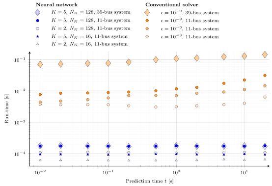
Figure 1: Run-time as a function of the prediction time $t$ for NNs of different size and a conventional solver with varied tolerance settings $\epsilon$. Tests for the 11-bus and 39-bus system with a disturbance $P_{i}=$6.09\text{\,}\mathrm{p.u.}$$.

First, for NNs the run-time is independent of the prediction time as the prediction only requires a single evaluation of the NN. In contrast, the conventional solver’s run-time increases with larger prediction times as more internal time steps are required. Second, the power system size strongly affects the conventional solver’s run-time as shown by the increase when moving from the 11-bus to the 39-bus system. For the NN, it causes only a negligible change in run-time as only the last layer of the NN changes in size according to the number of states of the system, see 3c. Third, the solver settings play an important role; for conventional solvers, the internal tolerance setting $\epsilon$ governs its evaluation speed, while for the NN the size, i.e., its number of layers $K$ and number of neurons per layer $N_{K}$, determine the run-time.

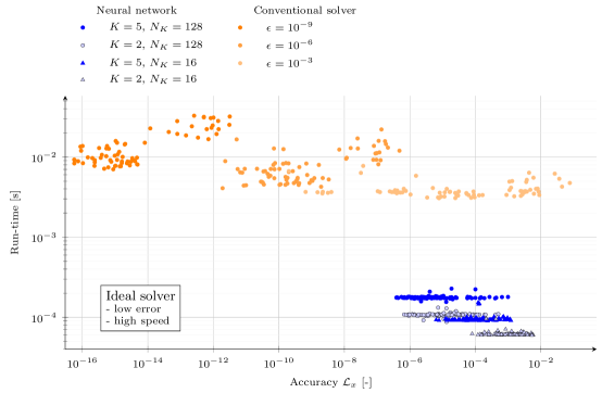
Figure 2: Evaluation of run-time and accuracy for the 11-bus system for varied solver tolerances $\epsilon$ and NN sizes ($K$ layers and $N_{K}$ neurons per layers). Point-wise evaluation for 10 disturbance sizes $P_{7}$ and prediction time as in Fig. 1.

Figure 2 sets the above results in relation to the achieved accuracy. The points represent different disturbance sizes and prediction times and the accuracy is measured as the associated loss. If a solver yielded points in the lower left corner of the plot, it could be called an ideal solver – fast and accurate. Conventional solvers can be very accurate when the internal tolerance $\epsilon$ is set low enough, but at the price of being slower to evaluate. Allowing larger tolerances accelerates the solution process slightly at the expense of less accurate solutions. However, this trade-off is limited by the numerical stability of the used scheme; for too high tolerances the results would be considered as non-converged. In case of NNs, their superior speed is weighed against less accurate solutions. The accuracy of NNs is not only controlled by their size but also, very importantly, by the training process. The achievable accuracy is therefore determined before run-time, in contrast to the tolerance of a conventional solver, which is set at run-time. As a final remark related to Figure 2, we need to highlight that while less adjustable, in contrast to conventional solvers, NNs do not face issues of numerical stability as their evaluation is a single and explicit function call.

We lastly want to show how the accuracy, here expressed as the maximum absolute error across all voltage angle states $\max\text{AE}_{\delta}$ for better intuition, relates to the NN size and the power system size. The boxplots in Fig. 3 represent the evaluation of 20 NNs with the same training setup but with different random initialisations of their parameters. We observe that deeper and wider NNs usually perform better on this metric. However, the largest NNs for the 11-bus system ($N_{K}=128$ and $K=4$ or $K=5$) show a larger variation than the smaller NN which means that the initialisation of the NNs affect their performance on the test dataset. This arises in models with a large representational capacity, loosely speaking models with many parameters, hence multiple parameter sets can lead to a low training loss but not all of them generalise well, i.e., have low error on the test dataset. The other, at first sight counter-intuitive, observation is that the 39-bus system performs better on the metric than the smaller 11-bus system. This can be attributed to the complexity of the target function, i.e., of the dynamic responses. The 11-bus system exhibits faster and more intricate dynamics for the presented cases, hence, it is more difficult to approximate their evolution. We could therefore achieve the same level accuracy for the 39-bus system with a smaller NN than for the 11-bus system. In terms of run-time, this would mean that the 39-bus system could be faster to evaluate than the 11-bus system. This characteristic of NNs effectively overcomes the relationship seen for conventional solvers that larger systems cause longer run-times as we have seen in Fig. 1.

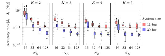
Figure 3: Maximum absolute error of angle $\delta$ on the test dataset for the 11-bus and 39-bus system with varying NN sizes, i.e., number of layers $K$ and neurons per layer $N_{K}$.

4.2 NNs at training time - a trade-off between accuracy and computational cost

The benefits of NNs compared to conventional solvers at run-time become possible by shifting the computational burden to the NN training stage, i.e., the pre-computation of the solution. In this stage, we examine the trade-off between accuracy and the computational cost of the training. This trade-off is influenced by several factors; here, we consider 1) the used training dataset, 2) the type of regularisation, and 3) the optimisation algorithm.

Table 2: Overview of the scenarios with different training datasets.

Scenario	Time increment $\Delta t$	Power disturbance increment $\Delta P$	Training dataset size $|\mathcal{D}_{\text{train}}|$	Dataset creation cost
A	$2\text{\,}\mathrm{s}$	$2\text{\,}\mathrm{p.u.}$	66	$0.413\text{\,}\mathrm{s}$
B	$1\text{\,}\mathrm{s}$	$2\text{\,}\mathrm{p.u.}$	126	$0.412\text{\,}\mathrm{s}$
C	$2\text{\,}\mathrm{s}$	$1\text{\,}\mathrm{p.u.}$	121	$0.812\text{\,}\mathrm{s}$
D	$1\text{\,}\mathrm{s}$	$1\text{\,}\mathrm{p.u.}$	231	$0.814\text{\,}\mathrm{s}$
E	$0.2\text{\,}\mathrm{s}$	$0.2\text{\,}\mathrm{p.u.}$	5151	$3.880\text{\,}\mathrm{s}$

To investigate the influence of the training dataset and the regularisation, we use the 11-bus system with a NN of size $K=5$ and $N_{K}=32$. We consider five scenarios as shown in Table 2 with different numbers of training data points $|\mathcal{D}_{\text{train}}|$ and the three flavours of NNs which we introduced in Section 2: vanilla NN, dtNN, PINN. The datasets are created by sampling with different increments of time $\Delta t$ and the power disturbance $\Delta P$. As expected, more data points incur a higher dataset creation cost, however, it also depends what kind of additional data points we generate. When we halve the time increment $\Delta t$, e.g., from scenario A to B or from scenario C to D, the dataset generation cost remains approximately the same. However, this does not hold if we halve the power increment $\Delta P$. When simulating a certain trajectory, it is basically free to evaluate additional points, i.e., reduce $\Delta t$, since interpolation schemes can be used for intermediate points. In contrast, any additional trajectory that needs to be simulated adds to the total cost. Similarly for free, we can obtain the necessary values for the dtNN regularisation as this only requires the evaluation of the right hand side in (2). The PINN regularisation also incurs only negligible dataset generation cost, as it is a mere sampling of the collocation points $|\mathcal{D}_{f}|$ without the need for any simulation (here, we use 5151 collocation points that are equally spaced and coincide with the data points from Scenario E). Hence, the additional regularisation comes at no or negligible cost compared to generating more data points unless they lie on trajectories that are evaluated anyways.

Figure 4a shows the resulting $\max\text{AE}_{\delta}$ across 20 training runs with different initialisations of the NN parameters. Unsurprisingly, the error metric improves with more data points, i.e., from scenario A to E, and additional regularisation, i.e., from a vanilla NN to a dtNN and a PINN. In scenario E, which has the largest dataset, all three network types perform on a similar level, whereas PINNs otherwise clearly deliver the best performance. Furthermore, the performance becomes more consistent, i.e., less variance, towards scenario E. A very sensitive issue is the point when to stop the training process to prevent over-fitting. In this study, we use the best validation loss as the indicator to determine the best epoch and Fig. 4b shows the results. PINNs consistently train for more epochs and only for scenario E the three NN types train for approximately the same number of epochs.

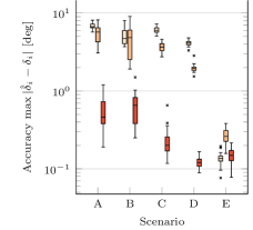
(a) Accuracy on the test dataset $\mathcal{D}_{\text{Test}}$

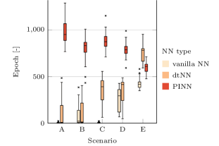
(b) Epoch with lowest $\mathcal{L}_{x}(\mathcal{D}_{\text{Validation}})$

Figure 4: Training characteristic for different scenarios (for scenario definition, see Table 2)

In Fig. 5 we plot the validation loss over the training epoch. In scenario D, we can clearly see, that while the vanilla NNs and the dtNNs do not improve much further after about 100 epochs, PINNs still see a significant improvement in terms of accuracy. From around this point onward, the physics-based loss $\mathcal{L}_{f}$ drives the optimisations, the other training loss terms are already very small. This behaviour partly stems from the fade-in of $\mathcal{L}_{f}$ but also from the fact that $\mathcal{L}_{x}$ and $\mathcal{L}_{dt}$ are based on much smaller datasets except for scenario E, in which the improvement of the accuracy progresses at similar speeds for all three NN types.

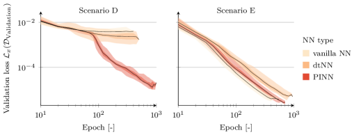
Figure 5: Validation loss as a function of trained epochs. The shadings signify the range from 20 randomly initialised runs.

PINNs offer us therefore the ability to achieve accuracy improvements for more epochs but we can also terminate them early if the achieved accuracy is sufficient to reduce the computational burden. By multiplying the number of epochs with the computational cost per epoch, we can estimate the total computational cost of the training. The vanilla NN and dtNN required about $0.17\text{\,}\mathrm{s}$ and $0.18\text{\,}\mathrm{s}$ per epoch for scenarios A-D and $0.40\text{\,}\mathrm{s}$ and $0.43\text{\,}\mathrm{s}$ for scenario E while the PINN constantly needs $0.66\text{\,}\mathrm{s}$ per epoch due to the collocation points. These numbers are very implementation and setup dependent, but show the trend that PINNs have higher cost per epoch due to the computation of $\mathcal{L}_{f}$ while the dtNN is only slightly more expensive than a vanilla NN. The total up-front cost, comprised of data generation cost and training cost, has then to be evaluated against the desired accuracy to find an efficient setup. This trade-off is again very dependent on the case study. For the 39-bus system the dataset generation cost is 2.5 times more while the cost per epoch only increases by a few percentage points.

Figures 3 and 4a displayed the maximum absolute errors on the test dataset as the accuracy metric, which is a critical metric of any solution approach. However, the accuracy of a NN must also be seen in dependence of the input domain, i.e., the input variables time $t$ and the disturbance size $P_{7}$.

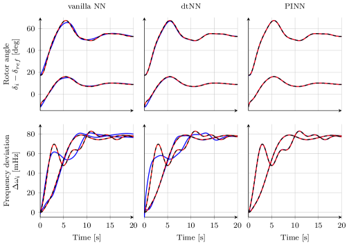
Figure 6: Trajectory of the angle and the frequency deviation at different buses (not the same for $\delta_{i}$ and $\Delta\omega_{i}$) based on a training with scenario A (blue) and scenario E (red). Ground truth is shown as the black dashed line and the three columns correspond to the three NN types.

To illustrate this dependence, we show in Fig. 6 predictions for the trajectories at two buses resulting from a disturbance of $P_{7}=$9.1\text{\,}\mathrm{p.u.}$$. The different NN types are trained based on scenario A (blue) and E (red) and the black dashed line represents ground truth. In the case of scenario A, NNs and dtNNs still show notable errors, whereas scenario E results in highly accurate predictions. For PINNs, already scenario A yields accurate results, which aligns with the observations in Fig. 4a.

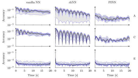
(a) Distribution of $\mathcal{L}_{x}(\mathcal{D}_{\text{Test}})$ as a function of the prediction time $t$

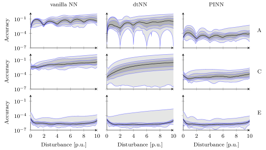
(b) Distribution of $\mathcal{L}_{x}(\mathcal{D}_{\text{Test}})$ as a function of the power disturbance size $P_{7}$

Figure 7: Distribution of $\mathcal{L}_{x}(\mathcal{D}_{\text{Test}})$ for different NN flavours (vanilla NN, dtNN, PINN) and scenarios (A,C,E). The shaded areas correspond to 100%, 80%, 50% of the errors and the black line represents the median. (for the definition of scenarios A, C, E, see Table 2)

Instead of considering a single disturbance size, we now analyse the prediction performance across the entire test dataset. To this end, we show in Fig. 7 the resulting distribution of the loss values as a function of the two input variables, i.e., the prediction time $t$ and the disturbance size $\Delta P_{i}$, for scenarios A, C, and E and the NN types. The plots clearly show that for a majority of points in the test dataset, the predictions are much more accurate than the maximum values. This is true in particular around the data points. These are clearly visible in scenario A by the indents. The panel for the dtNN and scenario C in Fig. 7a shows an extreme case where the prediction at the available data points is very accurate but the interpolation in between produces high errors. In comparison with the vanilla NN, the additional regularisation of the dtNN leads to a more unbalanced error distribution. In contrast, the PINN shows overall higher levels of accuracy but also more balanced error distributions thanks to the evaluation of the collocation points. We observe two more trends: Smaller prediction times are associated with higher errors due to the faster dynamics; and secondly, larger disturbances tend to show larger errors as they include larger variations of the output variables. These results show the importance of the dataset and the regularisation on the overall characteristics of a NN-based predictor, which must be considered for assessing the trade-off between training time and accuracy.

We lastly touch upon the effect of the optimiser on the training process, in this case the L-BFGS algorithm. The hyper-parameters of the algorithm strongly influence the required training time but also the achieved accuracy which is shown in Fig. 8. The points represent the outcome from random hyper-parameter settings and they clearly show a strong relationship between training time and accuracy. Furthermore, the optimiser’s internal tolerance setting (coloured) strongly influences this relationship.

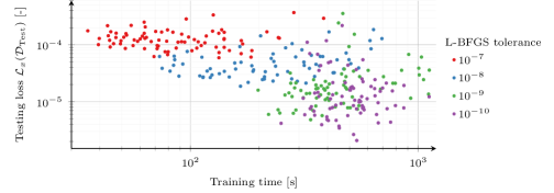
Figure 8: Influence of hyper-parameters of the L-BFGS-optimser on the trade-off between training time and achieved accuracy. The tolerance level of the optimiser has a large influence as shown by the coloured clusters of points.

5 Discussion

The results in the previous Section illustrate how NN-based approaches for solving DAEs offer a number of advantages at run-time: 10 to 1’000 times faster evaluation speed, no issues of numerical instability, and, in contrast to conventional solvers, their solution time does not increase with a growing power system size. These properties come at the cost of training the NNs. To assess an overall benefit in terms of computational time we, therefore, have to consider the total cost as the sum of up-front cost $C_{\text{up-front}}$ for the dataset generation and training and the run-time cost $C_{\text{run-time}}$ per evaluation $n$:

$$C_{\text{total}}=C_{\text{up-front}}+C_{\text{run-time}}\cdot n.$$ (17)

Figure 9 shows a graphical representation of 17 for classical solvers and NNs. It is clear, that NN-based approaches need to pass a critical number of evaluations $n_{\text{critical}}$ to be useful in terms of overall cost, unless other considerations like numerical stability or real-time applicability outweigh the cost consideration. The results in Sections 4.1 and 4.2 discussed the various settings that affect run and training time - in Fig. 9 they would correspond to the dashed lines. For classical solvers, changing these settings affects the slope, whereas for NNs they mostly impact the y-intercept, i.e., $C_{\text{up-front}}$; in either case, as expected, a different setting will change $n_{\text{critical}}$. Hence, the decision for using NN-based methods largely hinges around whether we expect sufficiently many evaluations $n$. Here, it is important to point out that the NN will be trained for a specific problem setup and a change in the setup, e.g., another network configuration, requires a new training process. In this aspect of flexibility, classical solvers have an important advantage over NN-based approaches.

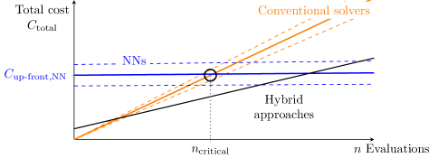
Figure 9: Total cost of different approaches in dependence of the number of evaluations.

Addressing this lack of flexibility is of paramount importance for adopting NNs-based simulation methods and we see three routes forward for this challenge: 1) Reducing the up-front cost $C_{\text{up-front}}$ by tailoring for example the learning algorithms, the used NN architectures, and regularisation schemes to the applications; this can largely be seen in the context of actively controlling the trade-off between accuracy and training time. 2) Finding use cases with large $n$, i.e., highly repetitive tasks. 3) Designing hybrid setups – similar to SAS-based methods – in which repetitive sub-problems are solved by NNs and classical solvers handle computations that require a lot of flexibility.

6 Conclusion

This paper presented a comprehensive analysis of the use of Physics-Informed Neural Network (PINN)for power system dynamic simulations. We show that PINNs (i) are 10 to 1’000 times faster than conventional solvers, (ii) do not face issues of numerical instability unlike conventional solvers, and, (iii) achieve a decoupling between the power system size and the required solution time. However, PINNs are less flexible (i.e. they do not easily handle parameter changes), and require an up-front training cost. Overall, this makes PINN-based solutions well-suited for repetitive tasks as well as task where run-time speed is crucial, such as for screening.

Besides the comparison between conventional and NN-based methods, this paper conducts a deeper analysis on the parameters that affect the performance of the NN solutions. In that respect, we introduce a new NN regularisation, called dtNN, as a intermediate step between NNs and PINNs. We show that PINNs achieve overall higher levels of accuracy, and more balanced error distributions thanks to the evaluation of the collocation points.

References

- [1] K. E. Brenan, S. L. Campbell, L. R. Petzold, Numerical Solution of Initial-Value Problems in Differential-Algebraic Equations, Society for Industrial and Applied Mathematics, 1995.
- [2] B. Stott, Power system dynamic response calculations, Proceedings of the IEEE 67 (2) (1979) 219–241. doi:10.1109/PROC.1979.11233.
- [3] P. W. Sauer, M. A. Pai, Power system dynamics and stability, Prentice Hall, Upper Saddle River, N.J, 1998.
- [4] G. Gurrala, et al., Parareal in Time for Fast Power System Dynamic Simulations, IEEE Transactions on Power Systems 31 (3) (2016) 1820–1830. doi:10.1109/TPWRS.2015.2434833.
- [5] Y. Liu, K. Sun, Solving Power System Differential Algebraic Equations Using Differential Transformation, IEEE Transactions on Power Systems 35 (3) (2020) 2289–2299. doi:10.1109/TPWRS.2019.2945512.
- [6] P. Aristidou, Time-domain simulation of large electric power systems using domain-decomposition and parallel processing methods, Ph.D. thesis, Université de Liège, Liège, Belgium (2015).
- [7] I. Lagaris, A. Likas, D. Fotiadis, Artificial neural networks for solving ordinary and partial differential equations, IEEE Transactions on Neural Networks 9 (5) (1998) 987–1000. doi:10.1109/72.712178.
- [8] M. Raissi, P. Perdikaris, G. E. Karniadakis, Physics-informed neural networks, Journal of Computational Physics 378 (C) (Nov. 2018). doi:10.1016/j.jcp.2018.10.045.
- [9] G. E. Karniadakis, et al., Physics-informed machine learning, Nature Reviews Physics 3 (6) (2021) 422–440. doi:10.1038/s42254-021-00314-5.
- [10] G. S. Misyris, A. Venzke, S. Chatzivasileiadis, Physics-Informed Neural Networks for Power Systems, in: 2020 IEEE Power & Energy Society General Meeting (PESGM), IEEE, Montreal, QC, Canada, 2020, pp. 1–5. doi:10.1109/PESGM41954.2020.9282004.
- [11] G. Gurrala, et al., Large Multi-Machine Power System Simulations Using Multi-Stage Adomian Decomposition, IEEE Transactions on Power Systems 32 (5) (2017) 3594–3606. doi:10.1109/TPWRS.2017.2655300.
- [12] N. Duan, K. Sun, Power System Simulation Using the Multistage Adomian Decomposition Method, IEEE Transactions on Power Systems 32 (1) (2017) 430–441. doi:10.1109/TPWRS.2016.2551688.
- [13] B. Wang, N. Duan, K. Sun, A Time–Power Series-Based Semi-Analytical Approach for Power System Simulation, IEEE Transactions on Power Systems 34 (2) (2019) 841–851. doi:10.1109/TPWRS.2018.2871425.
- [14] C. Moya, G. Lin, DAE-PINN: a physics-informed neural network model for simulating differential algebraic equations with application to power networks, Neural Computing and Applications 35 (5) (2023) 3789–3804. doi:10.1007/s00521-022-07886-y.
- [15] J. Li, M. Yue, Y. Zhao, G. Lin, Machine-Learning-Based Online Transient Analysis via Iterative Computation of Generator Dynamics, in: 2020 IEEE SmartGridComm, IEEE, Tempe, AZ, USA, 2020, pp. 1–6. doi:10.1109/SmartGridComm47815.2020.9302975.
-
[16]
W. Cui, W. Yang, B. Zhang, Predicting
Power System Dynamics and Transients: A Frequency Domain
Approach (Nov. 2021).
URL http://arxiv.org/abs/2111.01103 - [17] G. Cybenko, Approximation by superpositions of a sigmoidal function, Mathematics of Control, Signals, and Systems 2 (4) (1989) 303–314. doi:10.1007/BF02551274.
- [18] I. Goodfellow, Y. Bengio, A. Courville, Deep learning, Adaptive computation and machine learning, The MIT Press, Cambridge, Massachusetts, 2016.
- [19] A. G. Baydin, B. A. Pearlmutter, A. A. Radul, J. M. Siskind, Automatic Differentiation in Machine Learning: a Survey, Journal of Machine Learning Research 18 (153) (2018) 1–43.
- [20] T. Hastie, R. Tibshirani, J. Friedman, The Elements of Statistical Learning, Springer Series in Statistics, Springer, New York, NY, 2009.
- [21] P. Kundur, N. J. Balu, M. G. Lauby, Power system stability and control, The EPRI power system engineering series, McGraw-Hill, New York, 1994.
- [22] R. D. Zimmerman, C. E. Murillo-Sanchez, R. J. Thomas, MATPOWER: Steady-State Operations, Planning, and Analysis Tools for Power Systems Research and Education, IEEE Transactions on Power Systems 26 (1) (2011) 12–19. doi:10.1109/TPWRS.2010.2051168.
-
[23]
J. Stiasny, Publicly available implementation
(2023).
URL https://github.com/jbesty - [24] C. Andersson, C. Führer, J. Åkesson, Assimulo: A unified framework for ODE solvers, Mathematics and Computers in Simulation 116 (2015) 26–43. doi:10.1016/j.matcom.2015.04.007.
- [25] A. Paszke, et al., PyTorch: An Imperative Style, High-Performance Deep Learning Library, in: Advances in Neural Information Processing Systems, Vol. 32, Curran Associates, Inc., 2019, pp. 8024–8035.
-
[26]
L. Biewald, Experiment Tracking with Weights
and Biases, software available from wandb.com (2020).
URL https://www.wandb.com/ - [27] J. Stiasny, et al., Closing the Loop: A Framework for Trustworthy Machine Learning in Power Systems, in: Proceedings of the 11th Bulk Power Systems Dynamics and Control Symposium (IREP 2022), Banff, Canada, 2022, pp. 1–21. doi:10.48550/ARXIV.2203.07505.
- [28] S. Cuomo, et al., Scientific Machine Learning Through Physics–Informed Neural Networks: Where we are and What’s Next, Journal of Scientific Computing 92 (3) (2022) 88. doi:10.1007/s10915-022-01939-z.
-
[29]
X. Glorot, Y. Bengio,
Understanding the
difficulty of training deep feedforward neural networks, in: Proceedings of
the Thirteenth International Conference on Artificial Intelligence
and Statistics, JMLR Workshop and Conference Proceedings, 2010, pp.
249–256, iSSN: 1938-7228.
URL https://proceedings.mlr.press/v9/glorot10a.html