Reinforce Data, Multiply Impact: Improved Model Accuracy and Robustness with Dataset Reinforcement

Abstract

We propose Dataset Reinforcement, a strategy to improve a dataset once such that the accuracy of any model architecture trained on the reinforced dataset is improved at no additional training cost for users. We propose a Dataset Reinforcement strategy based on data augmentation and knowledge distillation. Our generic strategy is designed based on extensive analysis across CNN- and transformer-based models and performing large-scale study of distillation with state-of-the-art models with various data augmentations. We create a reinforced version of the ImageNet training dataset, called ImageNet⁺, as well as reinforced datasets CIFAR-100⁺, Flowers-102⁺, and Food-101⁺. Models trained with ImageNet⁺ are more accurate, robust, and calibrated, and transfer well to downstream tasks (e.g., segmentation and detection). As an example, the accuracy of ResNet-50 improves by 1.7% on the ImageNet validation set, 3.5% on ImageNetV2, and 10.0% on ImageNet-R. Expected Calibration Error (ECE) on the ImageNet validation set is also reduced by 9.9%. Using this backbone with Mask-RCNN for object detection on MS-COCO, the mean average precision improves by 0.8%. We reach similar gains for MobileNets, ViTs, and Swin-Transformers. For MobileNetV3 and Swin-Tiny, we observe significant improvements on ImageNet-R/A/C of up to 20% improved robustness. Models pretrained on ImageNet⁺ and fine-tuned on CIFAR-100⁺, Flowers-102⁺, and Food-101⁺, reach up to 3.4% improved accuracy. The code, datasets, and pretrained models are available at https://github.com/apple/ml-dr.

1 Introduction

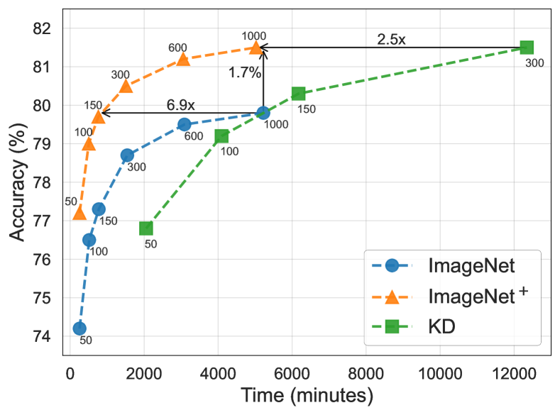
Figure 1: Reinforced ImageNet, ImageNet⁺, improves accuracy at similar iterations/wall-clock. ImageNet validation accuracy of ResNet-50 is shown as a function of training duration with (1) ImageNet dataset, (2) knowledge distillation (KD), and (3) ImageNet⁺ dataset (ours). Each point is a full training with epochs varying from 50-1000. An epoch has the same number of iterations for ImageNet/ImageNet⁺.

Model	+Data	+Reinforced	ImageNet	CIFAR-100	Flowers-102	Food-101
	Augmentation	Dataset(s)
MobileNetV3-Large	✗	✗	75.8	84.4	92.5	86.1
	✗	✓	77.9	87.5	95.3	89.5
ResNet-50	RandAugment	✗	80.4	88.4	93.6	90.0
	AutoAugment	✗	80.2	87.9	95.1	89.0
	TrivialAugWide	✗	80.4	87.9	94.8	89.3
	✗	✓	82.0	89.8	96.3	92.1
SwinTransformer-Tiny	RandAugment	✗	81.3	90.7	96.3	92.3
	✗	✓	84.0	91.2	97.0	92.9

Table 1: Training/fine-tuning on reinforced datasets improve accuracy for a variety of architectures. We reinforce each dataset once and train multiple models with similar cost as training on the original dataset. For datasets other than ImageNet, we fine-tune ImageNet/ImageNet⁺ pretrained models. Dataset reinforcement significantly benefits from efficiently reusing the knowledge of a teacher.

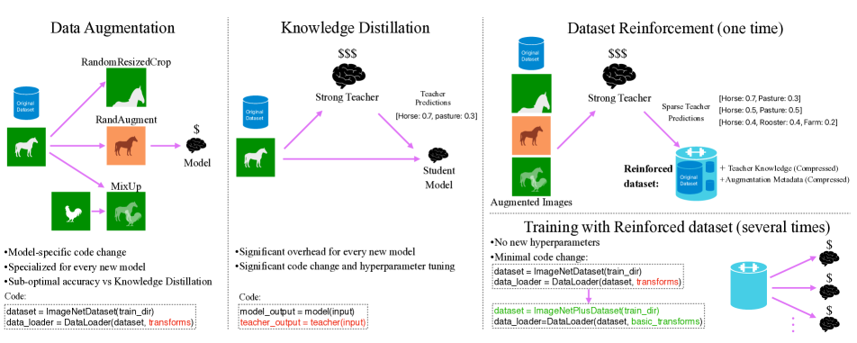
Figure 2: Illustration of Dataset Reinforcement. Data augmentation and knowledge distillation are common approaches to improving accuracy. Dataset reinforcement combines the benefits of both by bringing the advantages of large models trained on large datasets to other datasets and models. Training of new models with a reinforced dataset is as fast as training on the original dataset for the same total iterations. Creating a reinforced dataset is a one-time process (e.g., ImageNet to ImageNet⁺) the cost of which is amortized over repeated uses.

With the advent of the CLIP [47], the machine learning community got increasingly interested in massive datasets whereby the models are trained on hundreds of millions of samples, which is orders of magnitude larger than the conventional ImageNet [15] with 1.2M samples. At the same time, models have gradually grown larger in multiple domains [1]. In computer vision, the state-of-the-art models have upwards of $300$M parameters according to the Timm [63] library (e.g., BEiT [3], DeiT III [60], ConvNeXt [39]) and process inputs at up to $800\times 800$ resolution (e.g., EfficientNet-L2-NS [65]). Recent multi-modal vision-language models have up to 1.9B parameters (e.g., BeiT-3 [62]).

On the other side, there is a significant demand for small models that satisfy stringent hardware requirements. Additionally, there are plenty of tasks with small datasets that are challenging to scale because of the high cost associated with collecting and annotating new data. We seek to bridge this gap and bring the benefits of large models to any large, medium, or small dataset. We use knowledge from large models [47, 16, 7] to enhance the training of new models.

In this paper, we introduce Dataset Reinforcement (DR) as a strategy that improves the accuracy of models through reinforcing the training dataset. Compared to the original training data, a method for dataset reinforcement should satisfy the following desiderata:

• No overhead for users: Minimal increase in the computational cost of training a new model for similar total iterations (e.g., similar wall-clock time and CPU/GPU utilization).

• Minimal changes in user code and model: Zero or minimal modification to the training code and model architecture for the users of the reinforced dataset (e.g., only the dataset path and the data loader need to change).

• Architecture independence: Improve the test accuracy across variety of model architectures.

To understand the importance of the DR desiderata, let us discuss two common methods for performance improvements: data augmentation and knowledge distillation. Illustration in Fig. 2 compares these methods and our strategy for dataset reinforcement.

Data augmentation is crucial to the improved performance of machine learning models. Many state-of-the-art vision models [21, 27, 25] use the standard Inception-style augmentation [57] (i.e., random resized crop and random horizontal flipping) for training. In addition to these standard augmentation methods, recent models [59, 38] also incorporate mixing augmentations (e.g., MixUp [72] and CutMix [70]) and automatic augmentation methods (e.g., RandAugment [14] and AutoAugment [13]) to generate new data. However, data augmentation fails to satisfy all the desiderata as it does not provide architecture independent generalization. For example, light-weight CNNs perform best with standard Inception-style augmentations [25] while vision transformers [59, 38] prefer a combination of standard as well as advanced augmentation methods.

Knowledge distillation (KD) refers to the training of a student model by matching the output of a teacher model [35]. KD has consistently been shown to improve the accuracy of new models independent of their architecture significantly more than data augmentations [59]. However, knowledge distillation is expensive as it requires performing the inference (forward-pass) of an often significantly large teacher model at every training iteration. KD also requires modifying the training code to perform two forward passes on both the teacher and the student. As such, KD fails to satisfy minimal overhead and code change desiderata.

This paper proposes a dataset reinforcement strategy that exploits the advantages of both knowledge distillation and data augmentation by removing the training overhead of KD and finding generalizable data augmentations. Specifically, we introduce the ImageNet⁺ dataset that provides a balanced trade-off between accuracies on a variety of models and has the same wall-clock as training on ImageNet for the same number of iterations (Figs. 1 and 1). To train models using the ImageNet⁺ dataset, one only needs to change a few lines of the user code to use a modified data loader that reinforces every sample loaded from the training set.

Summary of contributions:

• We present a comprehensive large scale study of knowledge distillation from 80 pretrained state-of-the-art models and their ensembles. We observe that ensembles of state-of-the-art models trained on massive datasets generalize across student architectures (Sec. 2.1).

• We reinforce ImageNet by efficiently storing the knowledge of a strong teacher on a variety of augmentations. We investigate the generalizability of various augmentations for dataset reinforcement and find a tradeoff controlled by the reinforcement difficulty and model complexity (Sec. 2.2). This tradeoff can further be alleviated using curriculums based on the reinforcements (Sec. C.4).

• We introduce ImageNet⁺, a reinforced version of ImageNet, that provides up to 4% improvement in accuracy for a variety of architectures in short as well as long training. We show that ImageNet⁺ pretrained models result in 0.6-0.8 improvements in mAP for detection on MS-COCO and 0.3-1.3% improvement in mIoU for segmentation on ADE-20K (Sec. 3.1).

• Similarly, we create CIFAR-100⁺, Flowers-102⁺, and Food-101⁺, and demonstrate their effectiveness for fine-tuning (Sec. 2.3). ImageNet⁺ pretrained models fine-tuned on CIFAR-100⁺, Flowers-102⁺, and Food-101⁺ show up to 3% improvement in transfer learning on CIFAR-100, Flowers-102, and Food-101.

• To further investigate this emergent transferablity we study robustness and calibration of the ImageNet⁺ trained models. They reach up to 20% improvement on a variety of OOD datasets, ImageNet-(V2, A, R, C, Sketch), and ObjectNet (Sec. 3.2). We also show that models trained on ImageNet⁺ are well calibrated compared to their non-reinforced alternatives (Sec. 3.3).

Our ImageNet⁺, CIFAR-100⁺, Flowers-102⁺, and Food-101⁺ reinforcements along with code to reinforce new datasets are available at https://github.com/apple/ml-dr.

2 Dataset Reinforcement

Our proposed strategy for dataset reinforcement (DR) is efficiently combining knowledge distillation and data augmentation to generate an enhanced dataset. We precompute and store the output of a strong pretrained model on multiple augmentations per sample as reinforcements. The stored outputs are more informative and useful for training compared with ground truth labels. This approach is related to prior works, such as Fast Knowledge Distillation (FKD) [55]) and ReLabel [71], that aim to improve the labels. Beyond these works, our goal is to find generalizable reinforcements that improve the accuracy of any architecture. First we perform a comprehensive study to find a strong teacher (Sec. 2.1) then find generalizable reinforcements on ImageNet (Sec. 2.2). To demonstrate the generality of our strategy and findings, we further reinforce CIFAR-100, Flowers-102, and Food-101 (Sec. 2.3).

The reinforced dataset consists of the original dataset plus the reinforcement meta data for all training samples. During the reinforcement process, for each sample a fixed number of reinforcements is generated using parametrized augmentation operations and evaluating the teacher predictions. To save storage, instead of storing the augmented images, the augmentation parameters are stored alongside the sparsified output of the teacher. As a result, the extra storage needed is only a fraction of the original training set for large datasets. Using our reinforced dataset has no computational overhead on training, requires no code change, and provides improvements for various architectures.

2.1 What is a good teacher?

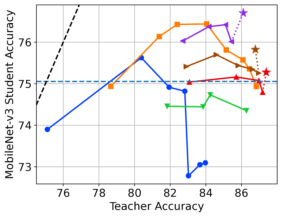
(a) Light-weight CNN (MobileNetV3)

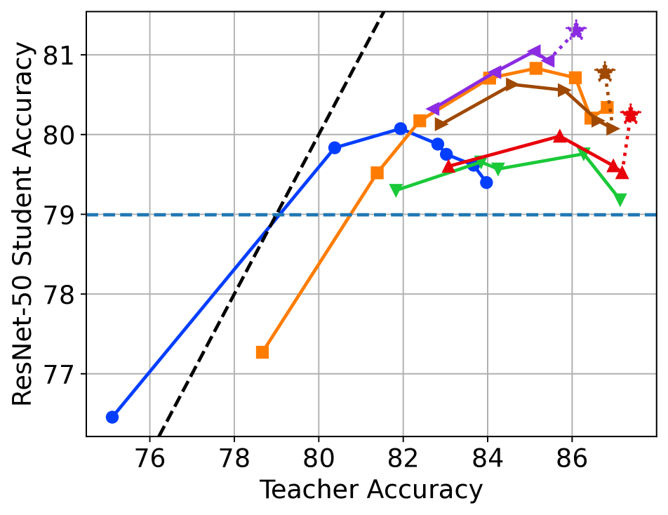
(b) Heavy-weight CNN (ResNet-50)

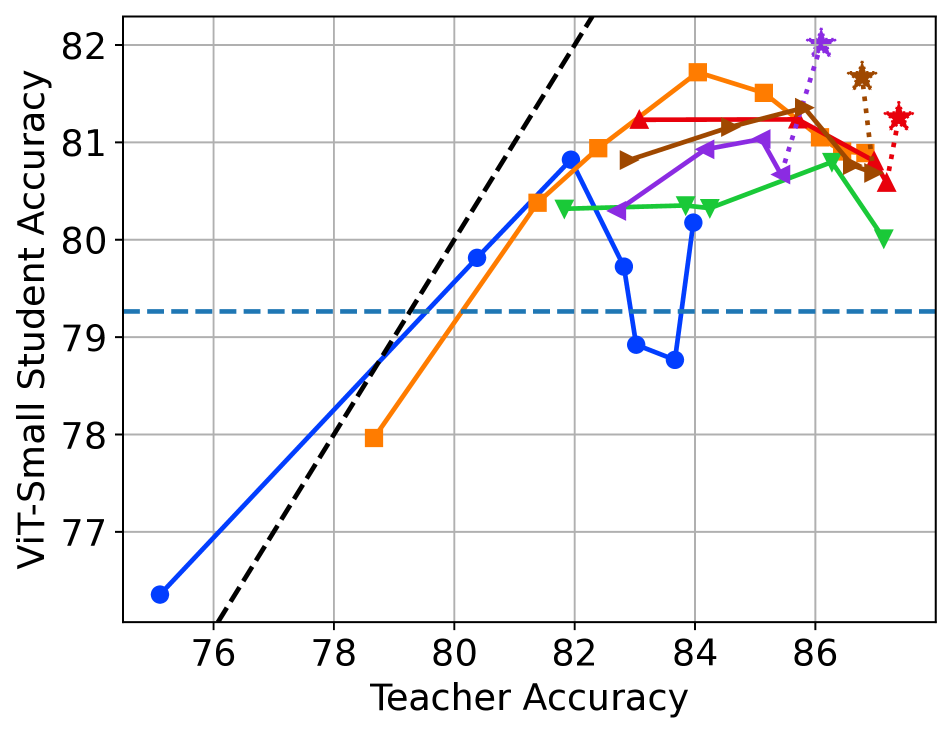
(c) Transformer (ViT-Small)

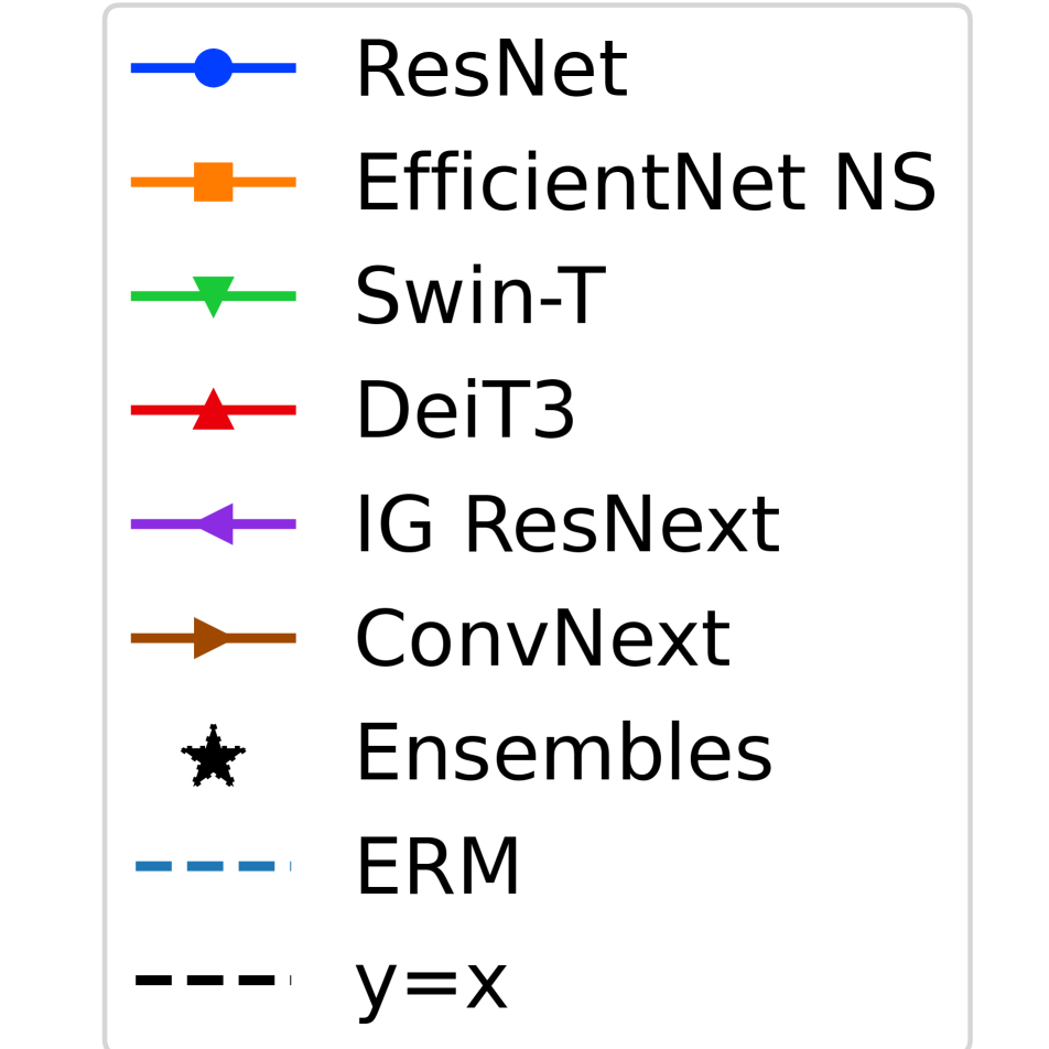
Figure 3: Knowledge Distillation with models and ensembles from Timm library. We observe the validation accuracy of students saturates or drops as the accuracy of teachers within an architecture family increases. We also observe that ensembles (marked by asterisks) are better teachers. Ensemble of IG-ResNext models performs best as teachers across student architectures. ERM (Empirical Risk Minimization) is standard training without knowledge distillation. Similar results for 150 epoch training in Fig. 7.

Knowledge distillation (KD) refers to training a student model using the outputs of a teacher model [9, 2, 35]. The training objective is as follows:

$$\min_{\theta}\,\mathbb{E}_{{\bm{x}}\sim\mathcal{D},\hat{{\bm{x}}}\sim\mathcal{A}({\bm{x}})}\mathcal{L}(f_{\theta}(\hat{{\bm{x}}}),g(\hat{{\bm{x}}}))\,,$$ (1)

where, $\mathcal{D}$ is the training dataset, $\mathcal{A}$ is augmentation function, $f_{\theta}$ is the student model parameterized with $\theta$, $g$ is the teacher model, and $\mathcal{L}$ is the loss function between student and teacher outputs. Throughout this paper, we use the KL loss without a temperature hyperparameter and no mixing with the cross-entropy loss. We teach the student to imitate the output of the teacher on all augmentations consistent with [6].

It is common to use a fixed teacher because repeating experiments and selecting the best teacher is expensive [6, 19]. The teacher is often selected based on the state-of-the-art test accuracy of available pretrained models. However, it has been observed that most accurate models do not necessarily appear to be the best teachers [12, 43]. Ensemble models on the other hand, have been shown to be promising teachers from the early work of [9] until recent works in various domains [10, 68, 54, 56] and with techniques to boost the their performance [52, 17, 41]. None of these works have comprehensively studied finding the best teacher along with the necessary augmentations that result in consistent improvements over multiple student architectures.

To understand what makes a good teacher to reinforce datasets, we perform knowledge distillation with a variety of pretrained models in the Timm library [63] distilled to three representative student architectures MobileNetV3-large [25], ResNet-50 [21], and ViT-Small [16]. MobileNetV3 represents light-weight CNNs that often prefer easier training. ResNet-50 represents heavy-weight CNNs that can benefit from difficult training regimes but do not heavily rely on it because of their implicit inductive bias of the architecture. ViT-small represents the transformer architectures that have less implicit bias compared with CNNs and learn better in the presence of complex and difficult datasets. We consider various families of models as teachers including ResNets (34–152 and type d variants) [21], ConvNeXt family pretrained on the ImageNet-22K and fine-tuned on ImageNet-1K [39], DeiT-3 pretrained on the ImageNet-21K and fine-tuned on ImageNet-1K, IG-ResNext pretrained on the Instagram dataset [40], EfficientNets with Noisy Student training [65], and Swin-TransformersV2 pretrained with and without ImageNet-22K and fine-tuned on ImageNet-1K [37]. This collection covers a variety of vision transformers and CNNs pretrained on a wide spectrum of dataset sizes. We train all students with $224\times 224$ inputs and follow [6] to match the resolution of teachers optimized to take larger inputs by passing the large crop to the teacher and resize it to $224\times 224$ for the student.

We present the accuracies of students trained for 300 epochs as a function of the teacher accuracy in Fig. 3. Focusing first on the single (non-ensemble) networks (marked by circles), consistent with prior work, we observe that the most accurate models are not usually the best teachers [43]. For CNN model families (ResNets, EfficientNets, ResNexts, and ConvNeXts), the student accuracy is generally correlated with the teacher accuracy. When increasing the teacher accuracy, the student first improves but then it starts to saturate or even drops with the most accurate member of the family. Vision Transformers (Swin-Transformers, and DeiT-3) as teachers do not show the same trend as the accuracy of the students flattens across different teachers. Recently,[36] suggested that temperature tuning can help in KD from larger teachers. We do not adopt such hyperparameter tuning strategies in favor of architecture-independence and generalizability of dataset reinforcement.

On the other side, ensembles of state-of-the-art models (marked by asterisks) are consistently better teachers compared with any individual member of the family. We create 4-member ensembles of the best models from IG-ResNexts, ConvNeXts, and DeiT3 to cover CNNs, vision transformers, and extra data models. We find IG-ResNext teacher to provide a balanced improvement across all students. IG-ResNext models are also trained with $224\times 224$ inputs while, for example, the best teacher from EfficientNet-NS family, EfficientNet-L2-NS, performs best at larger resolutions that is significantly more expensive to train with.

One of the benefits of dataset reinforcement paradigm is that the teacher can be expensive to train and use as long as we can afford to run it once on the target dataset for reinforcement. Also, the process of dataset reinforcement is highly parallelizable because performing the forward-pass on the teacher to generate predictions on multiple augmentations does not depend on any state or any optimization trajectory. For these reasons, we also considered significantly scaling knowledge distillation to super large ensembles with up to 128 members. We discuss our findings in Sec. B.2. Full table of accuracies for this section are in Sec. B.1.

2.2 ImageNet⁺: What is the best combination of reinforcements?

	Sparse teacher prob.	Random Resize Crop + Horizontal Flip	Random Augment + Random Erase	MixUp + CutMix
ImageNet+ variant	All	All	+RA/RE, +M*+R*	+Mixing, M*+R*
Apply probability	1	1, 0.5	1, 0.25	0.5, 0.5
Parameters	$10\times$ (Index, Prob)	$4\times$ Coords + Flip bit	$2\times$ (Op Id, Magnitude) + $4\times$ Coords	(Img Id, $\lambda$) + (Img Id, $4\times$ Coords)
Storage space (in bytes)	$10\times(2\times 4)$	$4\times 4+1$	$2\times 2\times 4+4\times 4$	$2\times 4+(1+4)\times 4$
Total storage space ($400$ samples per image)	38 GB	8 GB	15 GB	13 GB

Table 2: Additional storage in ImageNet⁺ variants. Total additional storage for ImageNet⁺ (RRC$+$RA/RE) is 61 GBs.

MobileNetV1	MobileNetV2	MobileNetV3	ImageNet+ Variants

(a) Light-weight CNNs

ResNet	EfficientNet

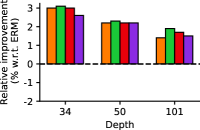
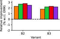
(b) Heavy-weight CNNs

ViT	SwinTransformer

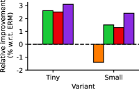
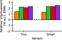
(c) Transformers

Figure 4: Improvements across architectures with ImageNet⁺ variants compared with ImageNet. Top-1 accuracy of different models on the ImageNet validation set consistently improves when trained with the proposed datasets as compared to the standard ImageNet training set (Epochs=150). Our proposed dataset variant with RRC$+$RA/RE, ImageNet⁺, provides balanced improvements of 1-4% across architectures. Further improvements with longer training (300-1000 epochs) in Tab. 4.

In this section, we introduce ImageNet⁺, a reinforcement of ImageNet. We create ImageNet⁺ using the IG-ResNext ensemble (Sec. 2.1). Following [55], we store top $10$ sparse probabilities for $400$ augmentations per training sample in the ImageNet dataset [15]. We consider the following augmentations: Random-Resize-Crop (RRC), MixUp [72] and CutMix [70] (Mixing), and RandomAugment [14] and RandomErase (RA/RE). We also combine Mixing with RA/RE and refer to it as M^∗$+$R^∗. We add all augmentations on top of RRC and for clarity add + as shorthand for RRC$+$. We provide a summary of the reinforcement data stored for each ImageNet⁺ variant in Tab. 2.

Models

We study light-weight CNN-based (MobileNetV1 [26]/ V2 [50]/ V3[25]), heavy-weight CNN-based (ResNet [21] and EfficientNet [58]), and transformer-based (ViT [16] and SwinTransformer [38]) models. We follow [42, 64] and use state-of-the-art recipes, including optimizers, hyperparameters, and learning schedules, specific to each model on the ImageNet. We perform no hyperparameter tuning specific to ImageNet⁺ and achieve improvements with the same setup as ImageNet for all models.

Better accuracy

We evaluate the performance of each model in terms of top-1 accuracy on the ImageNet validation set. Figure 4 compares the performance of different models trained using ImageNet and ImageNet⁺ datasets. Fig. 4(a) shows that light-weight CNN models do not benefit from difficult reinforcements. This is expected because of their limited capacity. On the other side, both heavy-weight CNN (Fig. 4(b)) and transformer-based (Fig. 4(c)) models benefit from difficult reinforcements (RRC$+$Mixing, RRC$+$RA/RE, and RRC$+$M^∗ $+$R^∗). However, transformer-based models deliver best performance with the most difficult reinforcement (RRC$+$M^∗ $+$R^∗). This concurs with previous works that show transformer-based models, unlike CNNs, benefit from more data regularization as they do not have inductive biases [16, 59].

Overall, RRC$+$RA/RE provides a balanced trade-off between performance and model size across different models. Therefore, in the rest of this paper, we use RRC$+$RA/RE as our reinforced dataset and call it ImageNet⁺. In the rest of the paper, we show results for three models that spans different model sizes and architecture designs (MobileNetV3-Large, ResNet-50, and SwinTransformer-Tiny).

We note that our observations are consistent across different architectures and recommend to see Appendix A for comprehensive results on 25 architectures. We provide expanded ablation studies in Appendix C using a cheaper teacher, ConvNext-Base-IN22FT1K. For example, we find 1) The number of stored samples can be $3\times$ fewer than intended training epochs, 2) Additional augmentations on top of ImageNet⁺ are not useful. 3) Tradeoff in reinforcement difficulty can be further reduced with curriculums. 4) Curriculums are better than various sample selection methods at the time of reinforcing the dataset. We provide all hyperparameters and training recipes in Appendix G.

2.3 CIFAR-100⁺, Flowers-102⁺, Food-101⁺: How to reinforce other datasets?

We reinforced ImageNet due to its popularity and effectiveness as a pretraining dataset for other tasks (e.g., object detection). Our findings on ImageNet are also useful for reinforcing other datasets and reduce the need for exhaustive studies. Specifically, we suggest the following guidelines: 1) use ensemble of strong teachers trained on large diverse data 2) balance reinforcement difficulty and model complexity.

In this section, we extend dataset reinforcement to three other datasets, CIFAR-100 [31], Flowers-102 [45], and Food-101 [8], with 50K, 1K, and 75K training data respectively. We build a teacher for each dataset by fine-tuning ImageNet⁺ pretrained ResNet-152 that reaches the accuracy of 90.6%, 96.6%, and 91.8%, respectively. By repeating fine-tuning 4 times, we get three teacher ensembles of 4xResNet-152. Next we generate reinforcements using similar augmentations to ImageNet⁺, that is RRC$+$RA/RE. We store 800, 8000, and 800 augmentations per original sample. After that, we train various models on the reinforced data at similar training time to standard training. To achieve the best performance, we use pretrained models on ImageNet/ImageNet⁺ and fine-tune on each dataset for varying epochs up to 1000, 10000, and 1000 (for CIFAR-100, Flowers-102, and Food-101, respectively) and report the best result.

Table 3 shows that MobileNetV3-Large pretrained and fine-tuned with reinforced datasets reaches up to 3% better accuracy. We observe that pretraining and fine-tuning on reinforced datasets together give the largest improvements. We provide results for other models in Appendix D.

Pretraining Dataset	CIFAR-100		Flowers-102		Food-101
	Orig.	+	Orig.	+	Orig.	+
None	80.2	83.6	68.8	87.5	85.1	88.2
ImageNet	84.4	87.2	92.5	94.1	86.1	89.2
ImageNet+ (Ours)	86.0	87.5	93.7	95.3	86.6	89.5

Table 3: Pretraining and fine-tuning on reinforced datasets is up to 3.4% better than using non-reinforced datasets. Top-1 accuracy on the test set for MobileNetV3-Large is shown. On Food-101, 86.1% is improved to 89.5%, demonstrating composition of reinforced datasets.

3 Experiments

Baseline methods

We compare the performance of models trained using ImageNet⁺ with the following baseline methods: (1) KD [35, 6] (Online distillation): A standard knowledge distillation method with strong teacher models and model-specific augmentations, (2) MEALV2 [54] (Fine-tuning distillation): Distill knowledge to student with good initialization from multiple teachers, (3) FunMatch [6] (Patient online distillation): Distill for significantly many epochs with strong augmentations, (4) ReLabel [71] (Offline label-map distillation): Pre-computes global label maps from the pre-trained teacher, and (5) FKD [55] (Offline distillation): Pre-computes soft labels using multi-crop knowledge distillation. We consider FKD as the baseline approach for dataset reinforcement.

Longer training

Recent works have shown that models trained for few epochs (e.g., 100 epochs) are sub-optimal and their performance improves with longer training [64, 16, 59]. Following these works, we train different models at three epoch budgets, i.e., 150, 300, and 1000 epochs, using both ImageNet and ImageNet⁺ datasets. Table 4 shows models trained with ImageNet⁺ dataset consistently deliver better accuracy in comparison to the ones trained on ImageNet. An epoch of ImageNet⁺ consists of exactly one random reinforcement per sample in ImageNet.

Model	Dataset	Training Epochs
		150	300	1000
MobileNetV3-Large	ImageNet	74.7	74.9	75.1
	ImageNet+ (Ours)	76.2	77.0	77.9
ResNet-50	ImageNet	77.4	78.8	79.6
	ImageNet+ (Ours)	79.6	80.6	81.7
SwinTransformer-Tiny	ImageNet	79.9	80.9	80.9
	ImageNet+ (Ours)	82.0	83.0	83.8

Table 4: ImageNet⁺ models consistently outperform ImageNet models when trained for longer. Top-1 accuracy on the ImageNet validation set is shown. An epoch has the same number of iterations for ImageNet/ImageNet⁺.

Training and reinforcement time

Table 4 shows ImageNet⁺ improves the performance of various models. A natural question that arises is: Does ImageNet⁺ introduce computational overhead when training models? On average, training MobileNetV3-Large, ResNet-50, and SwinTransformer-Tiny is $1.12\times$, $1.01\times$, and $0.99\times$ the total training time on ImageNet. The extra time for MobileNetV3 is because there is no data augmentations in our baseline. ImageNet⁺ took 2205 GPUh to generate using 64xA100 GPUs, which is highly parallelizable. For comparison, training ResNet-50 for 300 epochs on 8xA100 GPUs takes 206 GPUh. The reinforcement generation is a one-time cost that is amortized over many uses. The time to reinforce other datasets and the storage is discussed in Appendix F.

Model	Dataset	Offline	Random	Epochs	Accuracy
		KD?	Init.?
	ImageNet [25]	NA	✓	600	75.2
MobileNetV3	FunMatch [6]*	✗	✓	1200	76.3
-Large	MEALV2 [54]	✗	✗	180	76.9
	ImageNet+ (Ours)	✓	✓	300	77.0
ResNet-50	ImageNet [64]	NA	✓	600	80.4
	ReLabel [71]	✓	✓	300	78.9
	FKD [55]	✓	✓	300	80.1
	MEALV2 [54]	✗	✗	180	80.6
	ImageNet+ (Ours)	✓	✓	300	80.6
	ImageNet+ (Ours)	✓	✓	1000	81.7
	FunMatch [6]*	✗	✓	1200	81.8
ResNet-101	ImageNet [64]	NA	✓	1000	81.5
ViT-Tiny	ImageNet [59]	NA	✓	300	72.2
	DeiT [59]	✗	✓	300	74.5
	FKD [55]	✓	✓	300	75.2
	ImageNet+ (Ours)	✓	✓	300	75.8
ViT-Small	ImageNet [59]	NA	✓	300	79.8
	DeiT [59]	✗	✓	300	81.2
	ImageNet+ (Ours)	✓	✓	300	81.4
ViT-Base$\uparrow$384	ImageNet [59]	NA	✓	300	83.1
	DeiT [59]	✗	✓	300	83.4
	ImageNet+ (Ours)	✓	✓	300	84.5

Table 5: Comparison with state-of-the-art methods on the ImageNet validation set. Models trained with ImageNet⁺ dataset deliver similar or better performance than existing methods. Importantly, unlike online KD methods (e.g., FunMatch or DeiT), ImageNet⁺ does not add computational overhead to standard ImageNet training (Fig. 1). Here, NA denotes standard supervised ImageNet training with no online/offline KD. $\uparrow$384 denotes training at 384 resolution. An epoch has the same number of iterations for ImageNet/ImageNet⁺.

Comparison with state-of-the-art methods

Table 5 compares the performance of models trained with ImageNet⁺ and existing methods. We make following observations: (1) Compared to the closely related method, i.e., FKD, models trained using ImageNet⁺ deliver better accuracy. (2) We achieve comparable results to online distillation methods (e.g., FunMatch), but with fewer epochs and faster training (Fig. 1). (3) Small variants of the same family trained with ImageNet⁺ achieve similar performance to larger models trained with ImageNet dataset. For example, ResNet-50 (81.7%) with ImageNet⁺ achieves similar performance as ResNet-101 with ImageNet (81.5%). We observe similar phenomenon across other models, including light-weight CNN models. This enables replacing large models with smaller variants in their family for faster inference across devices, including edge devices, without sacrificing accuracy.

3.1 Transfer Learning

To evaluate the transferability of models pre-trained using ImageNet⁺ dataset, we evaluate on following tasks: (1) semantic segmentation with DeepLabv3 [11] on the ADE20K dataset [74], (2) object detection with Mask-RCNN [20] on the MS-COCO dataset [34], and (3) fine-grained classification on the CIFAR-100 [31], Flowers-102 [45], and Food-101 [8] datasets.

Tables 6 and 8 show models trained on the ImageNet⁺ dataset have better transferability properties as compared to the ImageNet dataset across different tasks (detection, segmentation, and fine-grained classification). To analyze the isolated impact of ImageNet⁺ in this section, the fine-tuning datasets are not reinforced. We present all combinations of training with reinforced/non-reinforced pretraining/fine-tuning datasets in Appendix D.

Model	Pretraining dataset	Task
		ObjDet	SemSeg
MobileNetV3-Large	ImageNet	35.5	37.2
	ImageNet+ (Ours)	36.1	38.5
ResNet-50	ImageNet	42.2	42.8
	ImageNet+ (Ours)	42.5	44.2
SwinTransformer-Tiny	ImageNet	45.8	41.2
	ImageNet+ (Ours)	46.5	42.5

Table 6: Transfer learning for object detection and semantic segmentation. For object detection (ObjDet), we report standard mean average precision on MS-COCO dataset while for sementic segmentation (SemSeg), we report mean intersection accuracy on ADE20K dataset. Task datasets are not reinforced.

3.2 Robustness analysis

To evaluate the robustness of different models trained using the ImageNet⁺ dataset, we evaluate on three subsets of the ImageNetV2 dataset [48], which is specifically designed to study the robustness of models trained on the ImageNet dataset. We also evaluate ImageNet models on other distribution shift datasets, ImageNet-A [24], ImageNet-R [22], ImageNet-Sketch [61], ObjectNet [4], and ImageNet-C [23]. We measure the top-1 accuracy except for ImageNet-C. On ImageNet-C, we measure the mean corruption error (mCE) and report 100 minus mCE.

Tab. 7 shows that models trained using ImageNet⁺ dataset are up to 20% more robust. Overall, these robustness results in conjunction with results in Tab. 4 highlight the effectiveness of the proposed dataset.

Model	Dataset	ImageNet-V2			ImageNet-A	ImageNet-R	ImageNet-Sketch	ObjectNet	ImageNet-C	Avg.
		V2-A	V2-B	V2-C
MobileNetV3-Large	ImageNet	71.5	62.9	76.8	4.5	32.4	20.6	32.8	21.8	30.4
	ImageNet+ (Ours)	75.1	66.3	80.5	7.6	42.0	29.0	38.1	32.0	37.1
ResNet-50	ImageNet	76.3	67.4	81.3	11.9	38.1	27.4	41.6	33.2	37.9
	ImageNet+ (Ours)	79.3	71.3	83.8	15.1	48.1	34.9	46.8	39.0	43.7
SwinTransformer-Tiny	ImageNet	77.0	69.3	81.6	21.0	37.7	25.4	40.5	36.9	39.6
	ImageNet+ (Ours)	81.5	74.1	85.3	30.2	58.0∗	40.8	50.6	46.6	51.1

Table 7: ImageNet⁺ models are up to 20% more robust on ImageNet distribution shifts. All models are trained for 1000 epochs. We report on ImageNetV2 variations Threshold-0.7 (V2-A), Matched-Frequency (V2-B), and Top-Images (V2-C). We report accuracy on all datasets except for ImageNet-C where we report 100 minus mCE metric. ^∗ Largest improvement.

Model	Pretraining dataset	Fine-tuning dataset
		CIFAR-100	Flowers-102	Food-101
MobileNetV3-Large	ImageNet	84.4	92.5	86.1
	ImageNet+ (Ours)	86.0	93.7	86.6
ResNet-50	ImageNet	88.4	93.6	90.0
	ImageNet+ (Ours)	88.8	95.0	90.5
SwinTransformer-Tiny	ImageNet	90.6	96.3	92.3
	ImageNet+ (Ours)	90.9	96.6	93.0

Table 8: Transfer learning for fine-grained object classification. Only pretraining dataset is reinforced and fine-tuning datasets are not reinforced. Reinforced pretraining/fine-tuning results in Tab. 1.

3.3 Calibration: Why are ImageNet⁺ models robust and transferable?

To understand why ImageNet⁺ models are significantly more robust than ImageNet models we evaluate their Expected Calibration Error (ECE) [32] on the validation set. Fig. 5 shows that ImageNet⁺ models are well-calibrated and significantly better than ImageNet models. This matches recent observations about ensembles that out-of-distribution robustness is better for well-calibrated models [33]. Full calibration results are presented in Appendix E.

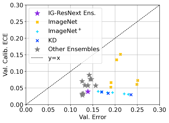
Figure 5: ImageNet⁺ models are well-calibrated. We plot the Expected Calibration Error (ECE) on the ImageNet validation set over the validation error (normalized by 100 to range $[0,1]$) for MobileNetV3/ResNet-50/Swin-Tiny architectures trained for 300 and 1000 epochs on ImageNet and ImageNet⁺. ImageNet⁺ models are significantly more calibrated, even matching or better than their teacher (IG-ResNext Ensemble). We also observe that the IG-ResNext model is one of the best calibrated models on the validation set from our pool of teachers.

3.4 Comparison with FKD and ReLabel.

We reproduce FKD and ReLabel with our training recipe as well as regenerate the dataset of FKD. We compare the accuracy on ImageNet validation and its distribution shifts as well as the cost of dataset generation/storage. We train models for 300 epochs.

Training recipe

We report results of training with our code on the released datasets of ReLabel and FKD. In addition to reproducing FKD results by training on their released dataset of 500-sample per image, we also reproduce their dataset using our code and their teacher. Tab. 9 verifies that our improvements are due to the superiority of ImageNet⁺, not any other factors such as the training recipe. Our ImageNet⁺-RRC is also closely related to FKD as it uses the same set of augmentations (random-resized-crop and horizontal flip) but together with our optimal teacher (4xIG-ResNext). We observe that ImageNet⁺-RRC achieves better results than FKD but still lower than ImageNet⁺ (Tabs. 11(c) and 4).

Generation/Storage Cost

We provide comparison of generation/storage costs in Tab. 9. In our reproduction, generating FKD’s data takes 2260 GPUh, slightly more than ImageNet⁺ because their teacher processes inputs at the larger resolution of $475\times 475$ compared to our resolution of $224\times 224$.

ImageNet⁺-Small

We subsampled ImageNet⁺ into a variant that is 10.6 GBs, comparable to prior work. We reduce the number of samples per image to 100 and store teacher probabilities with top-5 sparsity. If not subsampled from ImageNet⁺, generating ImageNet⁺-Small would take half the time of FKD (200 samples) while still comparable in accuracy to ImageNet⁺. Note that ImageNet⁺ is more general-purpose and preferred, especially for long training.

Dataset	Our	Our	Optimal		Top-K	Num.	Storage (GBs)		Gen. Time	ResNet-50		Swin-Tiny
	Gen.	Train	Teacher	Aug.		Samples	Raw	GZIP	(GPUh)	IN	IN-OOD	IN	IN-OOD
ReLabel	✗	✓	✗	✗	5	1	10.7	4.8	10	79.5	45.7	81.2	48.2
FKD	✗	✓	✗	✗	5	200	13.6	8.9	904∗	79.8	45.0	82.0	48.7
FKD	✗	✓	✗	✗	5	500	34.0	22.0	2260∗	80.1	45.0	82.2	48.9
FKD	✓	✓	✗	✗	10	400	46.3	33.4	1808	79.8	45.0	82.1	49.0
ImageNet+-RRC	✓	✓	✓	✗	10	400	46.3	33.4	1993	80.3	46.5	82.4	51.0
ImageNet+-Small	✓	✓	✓	✓	5	100	10.6	5.6	551	80.6	48.9	82.9	54.6
ImageNet+	✓	✓	✓	✓	10	400	61.5	37.5	2205	80.6	49.1	83.0	54.7

Table 9: Comparison with Relabel and FKD. Up to 5.6% better than FKD on ImageNet-OOD, the average of ImageNet-V2/A/R/S/O/C accuracies. Highlighted accuracies are within 0.2% of the best. Compared with prior work, we use an optimal teacher (4xIG-ResNext) and optimal combination of augmentations (RRC+RA/RE). ^∗ Our estimates.

3.5 CLIP-pretrained Teachers

In this section, we evaluate the performance of CLIP-pretrained models [47] fine-tuned on ImageNet as teachers. This study complements our large-scale study of teachers in Sec. 2.1 where we evaluated more than 100 SOTA large models and ensembles. Table 10 compares an ensemble of 4 CLIP-pretrained models to our selected ensemble of 4 IG-ResNext models as well as a mixture of ResNext, ConvNext, CLIP-ViT, and ViT (abrv. RCCV) models (See Appendix H for the model names). We generate new ImageNet⁺ variants and train various architectures for 1000 epochs on each dataset. We observe that ImageNet⁺ with our previously selected IG-ResNext ensemble is superior to CLIP-pretrained and mixed-architecture teachers across architectures. The CLIP variant provides near the maximum gain on Swin-Tiny and mixing it with IG-ResNext reduces the gap on CNNs.

Model	ImageNet	ImageNet+
		IG-ResNext∗	CLIP	Mixed
MobileNetV3-Large	${75.1}$	$\bm{77.9}_{\scriptscriptstyle+2.9}$	${77.2}_{\scriptscriptstyle+2.1}$	${77.4}_{\scriptscriptstyle+2.3}$
ResNet-50	${79.6}$	$\bm{81.7}_{\scriptscriptstyle+2.1}$	${81.1}_{\scriptscriptstyle+1.4}$	$\bm{81.5}_{\scriptscriptstyle+1.8}$
Swin-Tiny	${80.9}$	$\bm{83.8}_{\scriptscriptstyle+2.8}$	$\bm{83.7}_{\scriptscriptstyle+2.7}$	$\bm{83.8}_{\scriptscriptstyle+2.8}$

Table 10: Our selected IG-ResNext ensemble is superior to CLIP-pretrained ensembles. We reinforce ImageNet dataset with an ensemble of CLIP-pretrained models as well as a mixture of multiple architectures and train various models for 1000 epochs. Subscripts show the improvement on top of the ImageNet accuracy. ^∗ Our chosen ImageNet⁺ variant.

4 Related work

We build on top of the well-known Knowledge Distillation framework [9, 2, 35], the effectiveness of which has been extensively studied [12, 56]. Numerous variants of KD have been proposed, including feature distillation [28, 73], iterative distillation [43, 67], and self-distillation [65, 44, 18, 29]. Label smoothing, an effective regularizer and related to KD, is particularly related to our work when interpreted as augmenting the output space [69, 53].

Closely related to our work, investigating and improving the accuracy on the ImageNet dataset has attracted much interest lately. [5] eliminated erroneous labeled examples in the training with reference to a strong classifier. In [51], ImageNet dataset evaluation was revisited and alternative test sets were released. Relabel [71] proposed storing multiple labels on various regions of an image using a teacher. FKD [55] further pushed this direction by caching the predictions of a strong teacher but with a limited augmentation. Similarly, in [49], the architecture-independent generalization of KD was exploited to propose a unified scheme for training with ImageNet seamlessly without any hyperparameter tuning or per-model training recipes. [36] identified the temperature hyperparameter in KD as an important factor limiting benefits of stronger augmentations and teachers, and proposed an adaptive scheme to dynamically set the temperature during training. Distilling feature maps and probability distributions between the random pair of original images and their MixUp images was proposed to guide the network to learn cross-image knowledge [46, 66]. For self-supervised learning, [30] adapted modern image-based regularizations with KD to improve the contrastive loss with some supervision. Our work has also been inspired by [6] where they proposed imitating the teacher on severe augmentations and train for thousands of epochs. With our proposed DR strategy, we significantly reduce the cost of function matching by storing a few samples and reusing them for longer training.

5 Conclusion

We go beyond the conventional online knowledge distillation and introduce Dataset Reinforcement (DR) as a general offline strategy. Our investigation unwraps tradeoffs in finding generalizable reinforcements controlled by the difficulty of augmentations and we propose ways to balance.

We study the choice of the teacher (more than 100 SOTA large models and ensembles), augmentation (4 more than prior work), and their impact on a diverse collection of models (25 architectures), especially for long training (up to 1000 epochs). We demonstrate significant improvements (up to 20%) in robustness, calibration and transfer (in/out of distribution classification, segmentation, and detection). Our novel method of training and fine-tuning on doubly reinforced datasets (e.g., ImageNet⁺ to CIFAR-100⁺) demonstrates new possibilities of DR as a generic strategy. We also study ideas that were not used in ImageNet⁺, including curriculums, mixing augmentations and more in the appendix.

The proposed DR strategy is only an example of the large category of ideas possible within the scope of dataset reinforcement. Our desiderata would also be satisfied by methods that expand the training data, especially in limited data domains, using strong generative foundation models.

Limitations

Limitations of the teacher can potentially transfer through dataset reinforcement. For example, over-confident biased teachers should not be used and diverse ensembles are preferred. Human verification of the reinforcements is also a solution. Note that original labels are unmodified in reinforced datasets and can be used in curriculums. Our robustness and transfer learning evaluations consistently show better transfer and generalization for ImageNet⁺ models likely because of lower bias of the teacher ensemble trained on diverse data.

Acknowledgments

We would like to thank Arsalan Farooq, Farzad Abdolhosseini, Keivan Alizadeh-Vahid, Pavan Kumar Anasosalu Vasu, and Raviteja Vemulapalli for the enriching discussions. We also thank the reviewers for their valuable feedback.

Appendix A Full results of training on ImageNet and ImageNet⁺, compared with Knowledge Distillation

Table 11 provides the full results of training with ImageNet⁺ compared with ImageNet and Knowledge Distillation (KD). We choose RRC$+$RA/RE that provides a balanced trade-off across architectures and training durations, and call it ImageNet⁺. Results in Tab. 11 are without some state-of-the-art training features that are further improved in Tab. 12.

Table 12 provides improved results using state-of-the-art training recipes from the CVNets library [42]. We use the exact same ImageNet⁺ variant and only write a new dataset class in CVNets, further confirming our minimal code change claim. We note the training changes that help each model:

• Higher resolution training: EfficientNets, ViT-Base, Swin-Base. We observe that ImageNet⁺ reinforcements are resolution independent and provide improvements even if the resolution is different from the one used to generate them.

• Variable resolution with variable batch size training (VBS): ViTs, EfficientNets, Swin.

• Mixed-precision: ViTs, Swin.

• Multi-node training: EfficientNets (resolution larger than 224).

• Exponential Model Averaging (EMA): MobileViTs.

• New results for MobileViT.

Model	ImageNet	KD	RRC	RRC+Mixing	RRC+RA/RE	RRC+M*+R*
MobileNetv1-0.25	$54.5$	${56.5}_{\scriptscriptstyle+2.0}$	${\bm{56.5}_{\scriptscriptstyle+2.0}}$	${55.2}_{\scriptscriptstyle+0.7}$	${55.7}_{\scriptscriptstyle+1.2}$	${53.9}_{\scriptscriptstyle-0.6}$
MobileNetv1-0.5	$66.3$	${66.3}_{\scriptscriptstyle-0.0}$	${\bm{67.6}_{\scriptscriptstyle+1.3}}$	${67.1}_{\scriptscriptstyle+0.8}$	${66.9}_{\scriptscriptstyle+0.6}$	${66.3}_{\scriptscriptstyle-0.0}$
MobileNetv1-1.0	$73.6$	${74.6}_{\scriptscriptstyle+1.0}$	${\bm{75.2}_{\scriptscriptstyle+1.6}}$	${\bm{75.0}_{\scriptscriptstyle+1.4}}$	${\bm{75.0}_{\scriptscriptstyle+1.4}}$	${74.3}_{\scriptscriptstyle+0.7}$
MobileNetv2-0.25	$54.3$	${56.9}_{\scriptscriptstyle+2.6}$	${\bm{55.8}_{\scriptscriptstyle+1.5}}$	${54.1}_{\scriptscriptstyle-0.2}$	${53.8}_{\scriptscriptstyle-0.5}$	${52.5}_{\scriptscriptstyle-1.8}$
MobileNetv2-0.5	$65.3$	${66.2}_{\scriptscriptstyle+0.9}$	${\bm{66.0}_{\scriptscriptstyle+0.7}}$	${65.7}_{\scriptscriptstyle+0.4}$	${\bm{65.8}_{\scriptscriptstyle+0.4}}$	${64.0}_{\scriptscriptstyle-1.3}$
MobileNetv2-1.0	$72.7$	${72.8}_{\scriptscriptstyle+0.1}$	${\bm{73.8}_{\scriptscriptstyle+1.1}}$	${73.5}_{\scriptscriptstyle+0.8}$	${73.5}_{\scriptscriptstyle+0.8}$	${72.9}_{\scriptscriptstyle+0.2}$
MobileNetv3-Small	$66.3$	${65.8}_{\scriptscriptstyle-0.5}$	${\bm{68.0}_{\scriptscriptstyle+1.7}}$	${67.1}_{\scriptscriptstyle+0.8}$	${67.3}_{\scriptscriptstyle+1.0}$	${66.4}_{\scriptscriptstyle+0.2}$
MobileNetv3-Large	$74.7$	${75.5}_{\scriptscriptstyle+0.9}$	${\bm{76.0}_{\scriptscriptstyle+1.4}}$	${\bm{76.0}_{\scriptscriptstyle+1.4}}$	${\bm{76.2}_{\scriptscriptstyle+1.6}}$	${75.5}_{\scriptscriptstyle+0.8}$
ResNet-18	$67.8$	${72.1}_{\scriptscriptstyle+4.3}$	${\bm{72.3}_{\scriptscriptstyle+4.5}}$	${71.7}_{\scriptscriptstyle+4.0}$	${71.9}_{\scriptscriptstyle+4.1}$	${71.0}_{\scriptscriptstyle+3.2}$
ResNet-34	$73.2$	${76.4}_{\scriptscriptstyle+3.2}$	${\bm{76.2}_{\scriptscriptstyle+3.0}}$	${\bm{76.3}_{\scriptscriptstyle+3.1}}$	${\bm{76.2}_{\scriptscriptstyle+3.0}}$	${75.8}_{\scriptscriptstyle+2.6}$
ResNet-50	$77.4$	${80.3}_{\scriptscriptstyle+2.9}$	${\bm{79.6}_{\scriptscriptstyle+2.3}}$	${\bm{79.7}_{\scriptscriptstyle+2.3}}$	${\bm{79.6}_{\scriptscriptstyle+2.3}}$	${\bm{79.6}_{\scriptscriptstyle+2.2}}$
ResNet-101	$79.8$	${81.7}_{\scriptscriptstyle+1.9}$	${81.2}_{\scriptscriptstyle+1.4}$	${\bm{81.7}_{\scriptscriptstyle+1.8}}$	${\bm{81.5}_{\scriptscriptstyle+1.7}}$	${81.3}_{\scriptscriptstyle+1.5}$
ResNet-152	$80.8$	${82.3}_{\scriptscriptstyle+1.4}$	${81.6}_{\scriptscriptstyle+0.8}$	${\bm{82.0}_{\scriptscriptstyle+1.2}}$	${\bm{82.0}_{\scriptscriptstyle+1.1}}$	${\bm{81.9}_{\scriptscriptstyle+1.0}}$
EfficientNet-B2	$77.9$	${80.0}_{\scriptscriptstyle+2.1}$	${80.2}_{\scriptscriptstyle+2.3}$	${\bm{80.6}_{\scriptscriptstyle+2.7}}$	${\bm{80.7}_{\scriptscriptstyle+2.7}}$	${80.4}_{\scriptscriptstyle+2.4}$
EfficientNet-B3	$79.3$	${80.9}_{\scriptscriptstyle+1.6}$	${81.1}_{\scriptscriptstyle+1.8}$	${\bm{81.5}_{\scriptscriptstyle+2.2}}$	${\bm{81.6}_{\scriptscriptstyle+2.3}}$	${\bm{81.5}_{\scriptscriptstyle+2.2}}$
EfficientNet-B4	$79.4$	${81.8}_{\scriptscriptstyle+2.4}$	${81.0}_{\scriptscriptstyle+1.6}$	${\bm{81.3}_{\scriptscriptstyle+1.9}}$	${\bm{81.5}_{\scriptscriptstyle+2.1}}$	${\bm{81.3}_{\scriptscriptstyle+1.9}}$
ViT-Tiny	$71.5$	${72.0}_{\scriptscriptstyle+0.5}$	${71.5}_{\scriptscriptstyle+0.0}$	${74.1}_{\scriptscriptstyle+2.6}$	${74.0}_{\scriptscriptstyle+2.6}$	${\bm{74.6}_{\scriptscriptstyle+3.1}}$
ViT-Small	$78.4$	${80.2}_{\scriptscriptstyle+1.7}$	${77.0}_{\scriptscriptstyle-1.5}$	${79.9}_{\scriptscriptstyle+1.4}$	${79.7}_{\scriptscriptstyle+1.2}$	${\bm{80.8}_{\scriptscriptstyle+2.4}}$
Swin-Tiny	$79.9$	${81.7}_{\scriptscriptstyle+1.7}$	${81.3}_{\scriptscriptstyle+1.4}$	${\bm{82.1}_{\scriptscriptstyle+2.2}}$	${\bm{82.0}_{\scriptscriptstyle+2.1}}$	${\bm{82.2}_{\scriptscriptstyle+2.2}}$
Swin-Small	$80.6$	${83.4}_{\scriptscriptstyle+2.9}$	${81.9}_{\scriptscriptstyle+1.3}$	${\bm{82.9}_{\scriptscriptstyle+2.3}}$	${\bm{82.9}_{\scriptscriptstyle+2.4}}$	${\bm{83.1}_{\scriptscriptstyle+2.6}}$

(a) 150 epochs

Model	ImageNet	KD	RRC	RRC+Mixing	RRC+RA/RE	RRC+M*+R*
MobileNetv1-0.25	$55.7$	${57.4}_{\scriptscriptstyle+1.8}$	${\bm{56.8}_{\scriptscriptstyle+1.2}}$	${56.2}_{\scriptscriptstyle+0.5}$	${55.9}_{\scriptscriptstyle+0.3}$	${55.1}_{\scriptscriptstyle-0.6}$
MobileNetv1-0.5	$67.1$	${67.5}_{\scriptscriptstyle+0.4}$	${\bm{68.0}_{\scriptscriptstyle+1.0}}$	${67.7}_{\scriptscriptstyle+0.7}$	${\bm{68.0}_{\scriptscriptstyle+0.9}}$	${66.9}_{\scriptscriptstyle-0.1}$
MobileNetv1-1.0	$74.0$	${75.9}_{\scriptscriptstyle+1.9}$	${75.6}_{\scriptscriptstyle+1.6}$	${\bm{75.8}_{\scriptscriptstyle+1.8}}$	${\bm{75.9}_{\scriptscriptstyle+1.8}}$	${75.4}_{\scriptscriptstyle+1.3}$
MobileNetv2-0.25	$54.8$	${57.7}_{\scriptscriptstyle+2.9}$	${\bm{56.2}_{\scriptscriptstyle+1.4}}$	${55.2}_{\scriptscriptstyle+0.4}$	${54.9}_{\scriptscriptstyle+0.1}$	${53.1}_{\scriptscriptstyle-1.7}$
MobileNetv2-0.5	$66.0$	${66.9}_{\scriptscriptstyle+0.9}$	${\bm{67.2}_{\scriptscriptstyle+1.3}}$	${66.5}_{\scriptscriptstyle+0.5}$	${66.4}_{\scriptscriptstyle+0.5}$	${65.3}_{\scriptscriptstyle-0.7}$
MobileNetv2-1.0	$73.3$	${74.3}_{\scriptscriptstyle+1.0}$	${\bm{74.8}_{\scriptscriptstyle+1.5}}$	${74.2}_{\scriptscriptstyle+0.9}$	${74.5}_{\scriptscriptstyle+1.2}$	${73.9}_{\scriptscriptstyle+0.6}$
MobileNetv3-Small	$67.2$	${67.0}_{\scriptscriptstyle-0.2}$	${\bm{69.0}_{\scriptscriptstyle+1.8}}$	${68.1}_{\scriptscriptstyle+0.8}$	${68.2}_{\scriptscriptstyle+1.0}$	${67.1}_{\scriptscriptstyle-0.1}$
MobileNetv3-Large	$74.9$	${76.4}_{\scriptscriptstyle+1.5}$	${76.6}_{\scriptscriptstyle+1.7}$	${\bm{76.9}_{\scriptscriptstyle+2.0}}$	${\bm{77.0}_{\scriptscriptstyle+2.1}}$	${76.5}_{\scriptscriptstyle+1.6}$
ResNet-18	$68.7$	${73.5}_{\scriptscriptstyle+4.8}$	${\bm{72.7}_{\scriptscriptstyle+4.0}}$	${\bm{72.7}_{\scriptscriptstyle+4.0}}$	${\bm{72.7}_{\scriptscriptstyle+4.0}}$	${72.1}_{\scriptscriptstyle+3.4}$
ResNet-34	$74.3$	${77.9}_{\scriptscriptstyle+3.6}$	${76.9}_{\scriptscriptstyle+2.6}$	${\bm{77.3}_{\scriptscriptstyle+3.0}}$	${\bm{77.2}_{\scriptscriptstyle+2.9}}$	${76.9}_{\scriptscriptstyle+2.6}$
ResNet-50	$78.8$	${81.5}_{\scriptscriptstyle+2.8}$	${80.3}_{\scriptscriptstyle+1.5}$	${\bm{80.8}_{\scriptscriptstyle+2.0}}$	${\bm{80.6}_{\scriptscriptstyle+1.8}}$	${80.5}_{\scriptscriptstyle+1.7}$
ResNet-101	$80.9$	${83.0}_{\scriptscriptstyle+2.1}$	${81.8}_{\scriptscriptstyle+0.9}$	${\bm{82.3}_{\scriptscriptstyle+1.4}}$	${\bm{82.3}_{\scriptscriptstyle+1.4}}$	${\bm{82.4}_{\scriptscriptstyle+1.5}}$
ResNet-152	$81.5$	${83.4}_{\scriptscriptstyle+1.9}$	${82.5}_{\scriptscriptstyle+1.0}$	${\bm{83.0}_{\scriptscriptstyle+1.5}}$	${\bm{82.8}_{\scriptscriptstyle+1.3}}$	${\bm{82.9}_{\scriptscriptstyle+1.4}}$
EfficientNet-B2	$78.9$	${81.3}_{\scriptscriptstyle+2.3}$	${80.9}_{\scriptscriptstyle+1.9}$	${\bm{81.2}_{\scriptscriptstyle+2.3}}$	${\bm{81.2}_{\scriptscriptstyle+2.2}}$	${\bm{81.1}_{\scriptscriptstyle+2.2}}$
EfficientNet-B3	$80.1$	${82.1}_{\scriptscriptstyle+2.0}$	${81.7}_{\scriptscriptstyle+1.6}$	${\bm{82.2}_{\scriptscriptstyle+2.1}}$	${\bm{82.1}_{\scriptscriptstyle+2.0}}$	${\bm{82.1}_{\scriptscriptstyle+2.0}}$
EfficientNet-B4	$80.6$	${83.0}_{\scriptscriptstyle+2.3}$	${82.1}_{\scriptscriptstyle+1.5}$	${\bm{82.4}_{\scriptscriptstyle+1.8}}$	${\bm{82.3}_{\scriptscriptstyle+1.7}}$	${\bm{82.4}_{\scriptscriptstyle+1.7}}$
ViT-Tiny	$74.1$	${75.5}_{\scriptscriptstyle+1.4}$	${73.5}_{\scriptscriptstyle-0.6}$	${76.2}_{\scriptscriptstyle+2.0}$	${75.8}_{\scriptscriptstyle+1.7}$	${\bm{76.9}_{\scriptscriptstyle+2.7}}$
ViT-Small	$78.9$	${82.3}_{\scriptscriptstyle+3.4}$	${79.2}_{\scriptscriptstyle+0.2}$	${81.6}_{\scriptscriptstyle+2.7}$	${81.4}_{\scriptscriptstyle+2.4}$	${\bm{82.3}_{\scriptscriptstyle+3.3}}$
Swin-Tiny	$80.9$	${83.0}_{\scriptscriptstyle+2.1}$	${82.4}_{\scriptscriptstyle+1.5}$	${\bm{83.1}_{\scriptscriptstyle+2.2}}$	${\bm{83.0}_{\scriptscriptstyle+2.1}}$	${\bm{83.2}_{\scriptscriptstyle+2.3}}$
Swin-Small	$81.4$	${84.4}_{\scriptscriptstyle+3.0}$	${82.5}_{\scriptscriptstyle+1.1}$	${\bm{83.7}_{\scriptscriptstyle+2.3}}$	${\bm{83.9}_{\scriptscriptstyle+2.5}}$	${\bm{83.9}_{\scriptscriptstyle+2.5}}$

(b) 300 epochs

Model	ImageNet	RRC	RRC+Mixing	RRC+RA/RE	RRC+M*+R*
MobileNetv1-0.25	$56.7$	${\bm{57.6}_{\scriptscriptstyle+0.9}}$	${57.1}_{\scriptscriptstyle+0.4}$	${57.1}_{\scriptscriptstyle+0.4}$	${56.3}_{\scriptscriptstyle-0.4}$
MobileNetv1-0.5	$67.8$	${\bm{69.2}_{\scriptscriptstyle+1.4}}$	${68.8}_{\scriptscriptstyle+1.0}$	${68.5}_{\scriptscriptstyle+0.7}$	${68.0}_{\scriptscriptstyle+0.2}$
MobileNetv1-1.0	$74.1$	${76.4}_{\scriptscriptstyle+2.2}$	${\bm{76.7}_{\scriptscriptstyle+2.6}}$	${\bm{76.7}_{\scriptscriptstyle+2.5}}$	${76.4}_{\scriptscriptstyle+2.3}$
MobileNetv2-0.25	$55.7$	${\bm{56.7}_{\scriptscriptstyle+1.0}}$	${55.8}_{\scriptscriptstyle+0.1}$	${55.2}_{\scriptscriptstyle-0.5}$	${55.0}_{\scriptscriptstyle-0.7}$
MobileNetv2-0.5	$66.8$	${\bm{68.2}_{\scriptscriptstyle+1.4}}$	${67.3}_{\scriptscriptstyle+0.5}$	${67.1}_{\scriptscriptstyle+0.3}$	${65.9}_{\scriptscriptstyle-0.9}$
MobileNetv2-1.0	$73.9$	${\bm{75.4}_{\scriptscriptstyle+1.5}}$	${\bm{75.3}_{\scriptscriptstyle+1.4}}$	${\bm{75.5}_{\scriptscriptstyle+1.6}}$	${74.7}_{\scriptscriptstyle+0.8}$
MobileNetv3-Small	$67.9$	${69.0}_{\scriptscriptstyle+1.1}$	${68.4}_{\scriptscriptstyle+0.5}$	${\bm{69.4}_{\scriptscriptstyle+1.4}}$	${68.4}_{\scriptscriptstyle+0.4}$
MobileNetv3-Large	$75.1$	${77.2}_{\scriptscriptstyle+2.1}$	${77.4}_{\scriptscriptstyle+2.3}$	${\bm{77.9}_{\scriptscriptstyle+2.9}}$	${77.5}_{\scriptscriptstyle+2.4}$
ResNet-18	$69.9$	${73.6}_{\scriptscriptstyle+3.6}$	${\bm{73.9}_{\scriptscriptstyle+4.0}}$	${\bm{73.8}_{\scriptscriptstyle+3.8}}$	${73.3}_{\scriptscriptstyle+3.4}$
ResNet-34	$75.6$	${77.8}_{\scriptscriptstyle+2.2}$	${\bm{78.4}_{\scriptscriptstyle+2.8}}$	${\bm{78.4}_{\scriptscriptstyle+2.8}}$	${78.1}_{\scriptscriptstyle+2.6}$
ResNet-50	$79.6$	${81.1}_{\scriptscriptstyle+1.4}$	${\bm{81.8}_{\scriptscriptstyle+2.2}}$	${\bm{81.7}_{\scriptscriptstyle+2.1}}$	${\bm{81.8}_{\scriptscriptstyle+2.2}}$
ResNet-101	$81.4$	${82.7}_{\scriptscriptstyle+1.3}$	${\bm{83.6}_{\scriptscriptstyle+2.2}}$	${83.2}_{\scriptscriptstyle+1.8}$	${\bm{83.4}_{\scriptscriptstyle+2.0}}$
ResNet-152	$81.7$	${83.4}_{\scriptscriptstyle+1.7}$	${\bm{84.0}_{\scriptscriptstyle+2.3}}$	${\bm{83.8}_{\scriptscriptstyle+2.2}}$	${\bm{83.9}_{\scriptscriptstyle+2.3}}$
EfficientNet-B2	$79.3$	${81.5}_{\scriptscriptstyle+2.2}$	${\bm{81.9}_{\scriptscriptstyle+2.7}}$	${\bm{81.9}_{\scriptscriptstyle+2.7}}$	${\bm{81.7}_{\scriptscriptstyle+2.5}}$
EfficientNet-B3	$79.6$	${82.3}_{\scriptscriptstyle+2.7}$	${\bm{82.9}_{\scriptscriptstyle+3.3}}$	${\bm{82.8}_{\scriptscriptstyle+3.3}}$	${\bm{82.7}_{\scriptscriptstyle+3.2}}$
EfficientNet-B4	$81.2$	${82.9}_{\scriptscriptstyle+1.8}$	${\bm{83.2}_{\scriptscriptstyle+2.1}}$	${\bm{83.1}_{\scriptscriptstyle+1.9}}$	${\bm{83.2}_{\scriptscriptstyle+2.0}}$
ViT-Tiny	$75.9$	${76.6}_{\scriptscriptstyle+0.7}$	${\bm{78.5}_{\scriptscriptstyle+2.6}}$	${78.1}_{\scriptscriptstyle+2.1}$	${\bm{78.7}_{\scriptscriptstyle+2.8}}$
ViT-Small	$78.4$	${80.8}_{\scriptscriptstyle+2.4}$	${83.2}_{\scriptscriptstyle+4.8}$	${82.6}_{\scriptscriptstyle+4.2}$	${\bm{83.7}_{\scriptscriptstyle+5.3}}$
Swin-Tiny	$80.9$	${83.4}_{\scriptscriptstyle+2.5}$	${\bm{84.1}_{\scriptscriptstyle+3.1}}$	${83.8}_{\scriptscriptstyle+2.8}$	${\bm{84.0}_{\scriptscriptstyle+3.1}}$
Swin-Small	$81.9$	${83.9}_{\scriptscriptstyle+1.9}$	${84.5}_{\scriptscriptstyle+2.6}$	${84.4}_{\scriptscriptstyle+2.5}$	${\bm{84.8}_{\scriptscriptstyle+2.9}}$

(c) 1000 epochs

Table 11: Comparison of training different models using knowledge distillation and different ImageNet/ImageNet⁺ datasets. Subscripts show the improvement on top of the ImageNet accuracy. We highlight the best accuracy on each row from our proposed datasets and any number that is within $0.2$ of the best. Knowledge distillation results are not reported for E=1000 (Tab. 11(c)) as it is computationally very expensive.

Model	Base Recipes (Tab. 11)		CVNets		CVNets-EMA
	ImageNet	ImageNet+	ImageNet	ImageNet+	ImageNet	ImageNet+
MobileNetV1-0.25	${54.5}$	$\bm{55.7}_{\scriptscriptstyle+1.2}$	${55.2}$	${55.4}_{\scriptscriptstyle+0.2}$	${55.4}$	${55.4}_{\scriptscriptstyle+0.0}$
MobileNetV1-0.5	${66.3}$	$\bm{66.9}_{\scriptscriptstyle+0.6}$	${66.2}$	$\bm{67.1}_{\scriptscriptstyle+0.9}$	${66.4}$	$\bm{67.1}_{\scriptscriptstyle+0.7}$
MobileNetV1-1.0	${73.6}$	$\bm{75.0}_{\scriptscriptstyle+1.4}$	${73.5}$	$\bm{75.1}_{\scriptscriptstyle+1.5}$	${73.6}$	$\bm{75.1}_{\scriptscriptstyle+1.5}$
MobileNetV2-0.25	${54.3}$	${53.8}_{\scriptscriptstyle-0.5}$	$\bm{54.7}$	${54.2}_{\scriptscriptstyle-0.5}$	$\bm{54.7}$	${54.2}_{\scriptscriptstyle-0.5}$
MobileNetV2-0.5	${65.3}$	$\bm{65.8}_{\scriptscriptstyle+0.4}$	$\bm{65.7}$	$\bm{65.7}_{\scriptscriptstyle-0.0}$	$\bm{65.7}$	$\bm{65.7}_{\scriptscriptstyle+0.0}$
MobileNetV2-1.0	${72.7}$	${73.5}_{\scriptscriptstyle+0.8}$	${72.8}$	$\bm{73.8}_{\scriptscriptstyle+1.0}$	${72.8}$	$\bm{73.9}_{\scriptscriptstyle+1.1}$
MobileNetV3-Small	${66.3}$	${67.3}_{\scriptscriptstyle+1.0}$	${66.6}$	$\bm{67.7}_{\scriptscriptstyle+1.1}$	${66.7}$	$\bm{67.7}_{\scriptscriptstyle+1.1}$
MobileNetV3-Large	${74.7}$	${76.2}_{\scriptscriptstyle+1.6}$	${74.7}$	$\bm{76.5}_{\scriptscriptstyle+1.8}$	${74.8}$	$\bm{76.5}_{\scriptscriptstyle+1.7}$
MobileViT-XXSmall	-	-	${66.0}$	${67.4}_{\scriptscriptstyle+1.5}$	${66.7}$	$\bm{67.9}_{\scriptscriptstyle+1.2}$
MobileViT-XSmall	-	-	${72.6}$	${74.0}_{\scriptscriptstyle+1.4}$	${73.3}$	$\bm{74.7}_{\scriptscriptstyle+1.3}$
MobileViT-Small	-	-	${76.3}$	${78.3}_{\scriptscriptstyle+2.0}$	${76.7}$	$\bm{78.6}_{\scriptscriptstyle+1.9}$
ResNet-18	${67.8}$	${71.9}_{\scriptscriptstyle+4.1}$	${69.9}$	$\bm{73.2}_{\scriptscriptstyle+3.3}$	${69.8}$	$\bm{73.2}_{\scriptscriptstyle+3.4}$
ResNet-34	${73.2}$	${76.2}_{\scriptscriptstyle+3.0}$	${74.6}$	$\bm{76.9}_{\scriptscriptstyle+2.3}$	${74.7}$	$\bm{76.9}_{\scriptscriptstyle+2.3}$
ResNet-50	${77.4}$	${79.6}_{\scriptscriptstyle+2.3}$	${79.0}$	$\bm{80.3}_{\scriptscriptstyle+1.3}$	${79.1}$	$\bm{80.3}_{\scriptscriptstyle+1.2}$
ResNet-101	${79.8}$	${81.5}_{\scriptscriptstyle+1.7}$	${80.5}$	$\bm{81.8}_{\scriptscriptstyle+1.3}$	${80.5}$	$\bm{81.9}_{\scriptscriptstyle+1.3}$
ResNet-152	${80.8}$	${82.0}_{\scriptscriptstyle+1.1}$	${81.3}$	$\bm{82.2}_{\scriptscriptstyle+1.0}$	${81.3}$	$\bm{82.3}_{\scriptscriptstyle+0.9}$
EfficientNet-B2	${77.9}$	${80.7}_{\scriptscriptstyle+2.7}$	${79.5}$	$\bm{81.5}_{\scriptscriptstyle+2.1}$	${79.5}$	$\bm{81.6}_{\scriptscriptstyle+2.1}$
EfficientNet-B3	${79.3}$	${81.6}_{\scriptscriptstyle+2.3}$	${80.9}$	$\bm{82.4}_{\scriptscriptstyle+1.6}$	${80.8}$	$\bm{82.5}_{\scriptscriptstyle+1.6}$
EfficientNet-B4	${79.4}$	${81.5}_{\scriptscriptstyle+2.1}$	${82.7}$	$\bm{83.6}_{\scriptscriptstyle+1.0}$	${82.7}$	$\bm{83.7}_{\scriptscriptstyle+1.0}$
ViT-Tiny	${71.5}$	${74.0}_{\scriptscriptstyle+2.6}$	${72.1}$	$\bm{74.3}_{\scriptscriptstyle+2.2}$	${72.1}$	$\bm{74.4}_{\scriptscriptstyle+2.3}$
ViT-Small	${78.4}$	$\bm{79.7}_{\scriptscriptstyle+1.2}$	${78.4}$	$\bm{79.8}_{\scriptscriptstyle+1.4}$	${78.7}$	$\bm{79.9}_{\scriptscriptstyle+1.2}$
ViT-Base	-	-	${79.5}$	$\bm{81.7}_{\scriptscriptstyle+2.3}$	${80.6}$	$\bm{81.7}_{\scriptscriptstyle+1.1}$
ViT-384-Base	-	-	${80.5}$	$\bm{83.0}_{\scriptscriptstyle+2.5}$	${81.9}$	$\bm{83.1}_{\scriptscriptstyle+1.1}$
Swin-Tiny	${79.9}$	$\bm{82.0}_{\scriptscriptstyle+2.1}$	${80.5}$	$\bm{82.1}_{\scriptscriptstyle+1.6}$	${80.3}$	$\bm{81.9}_{\scriptscriptstyle+1.6}$
Swin-Small	${80.6}$	${82.9}_{\scriptscriptstyle+2.4}$	${82.2}$	$\bm{83.6}_{\scriptscriptstyle+1.4}$	${81.9}$	${83.3}_{\scriptscriptstyle+1.4}$
Swin-Base	-	-	${82.7}$	$\bm{83.9}_{\scriptscriptstyle+1.2}$	${82.2}$	$\bm{83.7}_{\scriptscriptstyle+1.4}$
Swin-384-Base	-	-	${82.6}$	$\bm{83.2}_{\scriptscriptstyle+0.6}$	${82.4}$	$\bm{83.0}_{\scriptscriptstyle+0.6}$

(a) 150 epochs

Model	Base Recipes (Tab. 11)		CVNets		CVNets-EMA
	ImageNet	ImageNet+	ImageNet	ImageNet+	ImageNet	ImageNet+
MobileNetV1-0.25	${55.7}$	${55.9}_{\scriptscriptstyle+0.3}$	${56.0}$	$\bm{56.5}_{\scriptscriptstyle+0.6}$	${56.1}$	$\bm{56.6}_{\scriptscriptstyle+0.5}$
MobileNetV1-0.5	${67.1}$	$\bm{68.0}_{\scriptscriptstyle+0.9}$	${67.0}$	$\bm{68.0}_{\scriptscriptstyle+1.0}$	${67.0}$	$\bm{68.1}_{\scriptscriptstyle+1.1}$
MobileNetV1-1.0	${74.0}$	$\bm{75.9}_{\scriptscriptstyle+1.8}$	${74.0}$	$\bm{76.0}_{\scriptscriptstyle+2.0}$	${74.1}$	$\bm{76.0}_{\scriptscriptstyle+1.9}$
MobileNetV2-0.25	${54.8}$	${54.9}_{\scriptscriptstyle+0.1}$	$\bm{55.4}$	${55.1}_{\scriptscriptstyle-0.3}$	$\bm{55.5}$	${55.1}_{\scriptscriptstyle-0.4}$
MobileNetV2-0.5	${66.0}$	$\bm{66.4}_{\scriptscriptstyle+0.5}$	${65.8}$	$\bm{66.5}_{\scriptscriptstyle+0.7}$	${65.9}$	$\bm{66.6}_{\scriptscriptstyle+0.7}$
MobileNetV2-1.0	${73.3}$	$\bm{74.5}_{\scriptscriptstyle+1.2}$	${73.7}$	$\bm{74.5}_{\scriptscriptstyle+0.8}$	${73.7}$	$\bm{74.5}_{\scriptscriptstyle+0.8}$
MobileNetV3-Small	${67.2}$	${68.2}_{\scriptscriptstyle+1.0}$	${67.4}$	$\bm{68.6}_{\scriptscriptstyle+1.2}$	${67.4}$	$\bm{68.5}_{\scriptscriptstyle+1.1}$
MobileNetV3-Large	${74.9}$	$\bm{77.0}_{\scriptscriptstyle+2.1}$	${74.9}$	$\bm{77.2}_{\scriptscriptstyle+2.3}$	${75.1}$	$\bm{77.2}_{\scriptscriptstyle+2.1}$
MobileViT-XXSmall	-	-	${67.5}$	${68.8}_{\scriptscriptstyle+1.3}$	${68.6}$	$\bm{69.7}_{\scriptscriptstyle+1.1}$
MobileViT-XSmall	-	-	${74.0}$	${75.6}_{\scriptscriptstyle+1.6}$	${74.9}$	$\bm{76.3}_{\scriptscriptstyle+1.4}$
MobileViT-Small	-	-	${77.3}$	${79.6}_{\scriptscriptstyle+2.3}$	${77.9}$	$\bm{80.1}_{\scriptscriptstyle+2.2}$
ResNet-18	${68.7}$	${72.7}_{\scriptscriptstyle+4.0}$	${71.2}$	$\bm{74.2}_{\scriptscriptstyle+3.0}$	${71.1}$	$\bm{74.2}_{\scriptscriptstyle+3.1}$
ResNet-34	${74.3}$	${77.2}_{\scriptscriptstyle+2.9}$	${75.6}$	$\bm{77.8}_{\scriptscriptstyle+2.1}$	${75.6}$	$\bm{77.8}_{\scriptscriptstyle+2.2}$
ResNet-50	${78.8}$	${80.6}_{\scriptscriptstyle+1.8}$	${79.6}$	$\bm{81.2}_{\scriptscriptstyle+1.6}$	${79.7}$	$\bm{81.2}_{\scriptscriptstyle+1.6}$
ResNet-101	${80.9}$	${82.3}_{\scriptscriptstyle+1.4}$	${81.3}$	$\bm{82.6}_{\scriptscriptstyle+1.3}$	${81.3}$	$\bm{82.7}_{\scriptscriptstyle+1.4}$
ResNet-152	${81.5}$	${82.8}_{\scriptscriptstyle+1.3}$	${81.8}$	$\bm{83.1}_{\scriptscriptstyle+1.3}$	${81.8}$	$\bm{83.1}_{\scriptscriptstyle+1.3}$
EfficientNet-B2	${78.9}$	${81.2}_{\scriptscriptstyle+2.2}$	${80.7}$	$\bm{82.1}_{\scriptscriptstyle+1.4}$	${80.8}$	$\bm{82.1}_{\scriptscriptstyle+1.3}$
EfficientNet-B3	${80.1}$	${82.1}_{\scriptscriptstyle+2.0}$	${81.8}$	$\bm{83.3}_{\scriptscriptstyle+1.5}$	${81.8}$	$\bm{83.3}_{\scriptscriptstyle+1.5}$
EfficientNet-B4	${80.6}$	${82.3}_{\scriptscriptstyle+1.7}$	${82.8}$	$\bm{84.4}_{\scriptscriptstyle+1.6}$	${82.7}$	$\bm{84.4}_{\scriptscriptstyle+1.7}$
ViT-Tiny	${74.1}$	$\bm{75.8}_{\scriptscriptstyle+1.7}$	${74.8}$	$\bm{76.0}_{\scriptscriptstyle+1.2}$	${74.9}$	$\bm{76.0}_{\scriptscriptstyle+1.1}$
ViT-Small	${78.9}$	$\bm{81.4}_{\scriptscriptstyle+2.4}$	${79.1}$	$\bm{81.4}_{\scriptscriptstyle+2.3}$	${79.9}$	$\bm{81.5}_{\scriptscriptstyle+1.5}$
ViT-Base	-	-	${78.6}$	$\bm{84.1}_{\scriptscriptstyle+5.5}$	${81.0}$	$\bm{84.1}_{\scriptscriptstyle+3.1}$
ViT-384-Base	-	-	${80.0}$	$\bm{84.5}_{\scriptscriptstyle+4.6}$	${82.6}$	$\bm{84.5}_{\scriptscriptstyle+1.9}$
Swin-Tiny	${80.9}$	$\bm{83.0}_{\scriptscriptstyle+2.1}$	${81.2}$	$\bm{83.2}_{\scriptscriptstyle+2.1}$	${80.8}$	${82.8}_{\scriptscriptstyle+2.0}$
Swin-Small	${81.4}$	${83.9}_{\scriptscriptstyle+2.5}$	${82.4}$	$\bm{84.4}_{\scriptscriptstyle+2.0}$	${82.2}$	${84.1}_{\scriptscriptstyle+1.9}$
Swin-Base	-	-	${82.7}$	$\bm{84.7}_{\scriptscriptstyle+2.0}$	${82.5}$	${84.4}_{\scriptscriptstyle+1.9}$
Swin-384-Base	-	-	${83.9}$	$\bm{84.4}_{\scriptscriptstyle+0.5}$	${83.7}$	$\bm{84.2}_{\scriptscriptstyle+0.5}$

(b) 300 epochs

Model	Base Recipes (Tab. 11)		CVNets		CVNets-EMA
	ImageNet	ImageNet+	ImageNet	ImageNet+	ImageNet	ImageNet+
MobileNetV1-0.25	${56.7}$	$\bm{57.1}_{\scriptscriptstyle+0.4}$	$\bm{56.9}$	$\bm{57.1}_{\scriptscriptstyle+0.2}$	$\bm{56.9}$	$\bm{57.1}_{\scriptscriptstyle+0.2}$
MobileNetV1-0.5	${67.8}$	${68.5}_{\scriptscriptstyle+0.7}$	${68.1}$	$\bm{68.7}_{\scriptscriptstyle+0.6}$	${68.1}$	$\bm{68.8}_{\scriptscriptstyle+0.7}$
MobileNetV1-1.0	${74.1}$	$\bm{76.7}_{\scriptscriptstyle+2.5}$	${74.1}$	$\bm{76.8}_{\scriptscriptstyle+2.7}$	${74.4}$	$\bm{76.8}_{\scriptscriptstyle+2.4}$
MobileNetV2-0.25	$\bm{55.7}$	${55.2}_{\scriptscriptstyle-0.5}$	$\bm{55.7}$	$\bm{55.7}_{\scriptscriptstyle-0.0}$	$\bm{55.8}$	$\bm{55.7}_{\scriptscriptstyle-0.1}$
MobileNetV2-0.5	${66.8}$	$\bm{67.1}_{\scriptscriptstyle+0.3}$	${66.8}$	$\bm{67.1}_{\scriptscriptstyle+0.3}$	${66.8}$	$\bm{67.2}_{\scriptscriptstyle+0.4}$
MobileNetV2-1.0	${73.9}$	$\bm{75.5}_{\scriptscriptstyle+1.6}$	${74.0}$	$\bm{75.5}_{\scriptscriptstyle+1.5}$	${74.1}$	$\bm{75.6}_{\scriptscriptstyle+1.5}$
MobileNetV3-Small	${67.9}$	$\bm{69.4}_{\scriptscriptstyle+1.4}$	${68.1}$	$\bm{69.6}_{\scriptscriptstyle+1.5}$	${68.1}$	$\bm{69.6}_{\scriptscriptstyle+1.5}$
MobileNetV3-Large	${75.1}$	$\bm{77.9}_{\scriptscriptstyle+2.9}$	${74.8}$	$\bm{77.9}_{\scriptscriptstyle+3.1}$	${75.8}$	$\bm{77.9}_{\scriptscriptstyle+2.1}$
MobileViT-XXSmall	-	-	${68.6}$	${69.5}_{\scriptscriptstyle+0.9}$	${70.3}$	$\bm{71.5}_{\scriptscriptstyle+1.2}$
MobileViT-XSmall	-	-	${74.8}$	${76.2}_{\scriptscriptstyle+1.4}$	${76.1}$	$\bm{77.5}_{\scriptscriptstyle+1.4}$
MobileViT-Small	-	-	${77.7}$	${80.5}_{\scriptscriptstyle+2.8}$	${79.2}$	$\bm{81.4}_{\scriptscriptstyle+2.2}$
ResNet-18	${69.9}$	${73.8}_{\scriptscriptstyle+3.8}$	${72.3}$	$\bm{75.0}_{\scriptscriptstyle+2.7}$	${72.2}$	$\bm{75.1}_{\scriptscriptstyle+2.9}$
ResNet-34	${75.6}$	${78.4}_{\scriptscriptstyle+2.8}$	${76.6}$	$\bm{78.8}_{\scriptscriptstyle+2.2}$	${76.6}$	$\bm{78.9}_{\scriptscriptstyle+2.3}$
ResNet-50	${79.6}$	${81.7}_{\scriptscriptstyle+2.1}$	${80.0}$	$\bm{82.0}_{\scriptscriptstyle+1.9}$	${80.1}$	$\bm{82.0}_{\scriptscriptstyle+1.9}$
ResNet-101	${81.4}$	${83.2}_{\scriptscriptstyle+1.8}$	${80.9}$	$\bm{83.5}_{\scriptscriptstyle+2.6}$	${81.4}$	$\bm{83.5}_{\scriptscriptstyle+2.1}$
ResNet-152	${81.7}$	$\bm{83.8}_{\scriptscriptstyle+2.2}$	${81.3}$	$\bm{83.9}_{\scriptscriptstyle+2.6}$	${82.0}$	$\bm{83.9}_{\scriptscriptstyle+2.0}$
EfficientNet-B2	${79.3}$	${81.9}_{\scriptscriptstyle+2.7}$	${81.1}$	$\bm{83.1}_{\scriptscriptstyle+2.0}$	${81.3}$	$\bm{83.2}_{\scriptscriptstyle+1.9}$
EfficientNet-B3	${79.6}$	${82.8}_{\scriptscriptstyle+3.3}$	${81.7}$	$\bm{83.9}_{\scriptscriptstyle+2.2}$	${82.1}$	$\bm{83.9}_{\scriptscriptstyle+1.8}$
EfficientNet-B4	${81.2}$	${83.1}_{\scriptscriptstyle+1.9}$	${82.2}$	$\bm{85.0}_{\scriptscriptstyle+2.9}$	${83.4}$	$\bm{85.0}_{\scriptscriptstyle+1.6}$
ViT-Tiny	${75.9}$	$\bm{78.1}_{\scriptscriptstyle+2.1}$	${76.7}$	$\bm{77.9}_{\scriptscriptstyle+1.2}$	${76.9}$	$\bm{78.0}_{\scriptscriptstyle+1.1}$
ViT-Small	${78.4}$	${82.6}_{\scriptscriptstyle+4.2}$	${78.5}$	$\bm{82.8}_{\scriptscriptstyle+4.2}$	${80.6}$	$\bm{82.9}_{\scriptscriptstyle+2.3}$
ViT-Base	-	-	${76.8}$	$\bm{85.1}_{\scriptscriptstyle+8.3}$	${80.8}$	$\bm{85.1}_{\scriptscriptstyle+4.3}$
ViT-384-Base	-	-	${79.4}$	$\bm{85.4}_{\scriptscriptstyle+6.0}$	${83.1}$	$\bm{85.5}_{\scriptscriptstyle+2.5}$
Swin-Tiny	${80.9}$	$\bm{83.8}_{\scriptscriptstyle+2.8}$	${81.3}$	$\bm{84.0}_{\scriptscriptstyle+2.7}$	${80.5}$	${83.5}_{\scriptscriptstyle+3.0}$
Swin-Small	${81.9}$	${84.4}_{\scriptscriptstyle+2.5}$	${81.3}$	$\bm{85.0}_{\scriptscriptstyle+3.7}$	${81.9}$	${84.5}_{\scriptscriptstyle+2.6}$
Swin-Base	-	-	${81.5}$	$\bm{85.4}_{\scriptscriptstyle+3.9}$	${81.8}$	$\bm{85.2}_{\scriptscriptstyle+3.5}$
Swin-384-Base	-	-	${83.6}$	$\bm{85.8}_{\scriptscriptstyle+2.2}$	${83.8}$	${85.5}_{\scriptscriptstyle+1.7}$

(c) 1000 epochs

Table 12: Improved results with state-of-the-art training recepies in CVNets library. Subscripts show the improvement on top of the ImageNet accuracy. We highlight the best accuracy on each row from our proposed datasets and any number that is within $0.2$ of the best.

A.1 Aggregated improvements of ImageNet⁺ across models

To better demonstrate the scale of accuracy improvements, we plot the results of training on ImageNet⁺ (RRC$+$RA/RE) from Tab. 11 in Fig. 6(a) (300 epochs). RRC$+$RA/RE balances the tradeoff between various architectures. Given prior knowledge of architecture characteristics or enough training resources, we can select the dataset optimal for any architecture. Figure 6(b) shows the best accuracy achieved for each model when we train on all 4 of our reinforced datasets for 300 epochs (maximum of the four numbers). We observe that alternative reinforced datasets can provide 1-2% additional improvement, especially for light-weight CNNs and Transformers. In practice, given the knowledge of the complexity of the model architecture, one can decide to use alternative datasets (RRC for light-weight and RRC$+$M^∗ $+$R^∗for heavy-weight models or Transformers). Otherwise, given additional compute resources, one can train on all 4 datasets and choose the best model according to the validation accuracy.

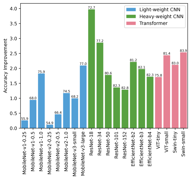
(a) ImageNet⁺ (RRC+RA/RE)

(b) Maximum of 4 ImageNet⁺ variants

Figure 6: ImageNet⁺ training improves validation accuracy compared with ImageNet training (Epochs=$300$). To train models using the ImageNet⁺ dataset, we use the same publicly-available ImageNet training recipes with no hyperparameter tuning on ImageNet⁺. We use the same hyperparameters tuned for ImageNet with no hyperparameter tuning on ImageNet⁺. ImageNet⁺ provides a balanced tradeoff with more improvements for Heavy-weight CNNs and Transformers. Figure 6(b): further improvements are achieved using the best out of our 4 proposed datasets (See Tab. 11(b) for details).

Appendix B Expanded study on what is a good teacher?

In this section we provide additional results and studies such as super ensembles as teachers.

B.1 Additional results of knowledge distillation with pretrained Timm models

Figure 7 (E=150) complements Fig. 3 (E=300) demonstrating the validation accuracy using knowledge distillation for a variety of teachers from the Timm library [63]. Table 13 shows the results in detail. For both 150 and 300 epoch training durations, we observe that ensembles of the state-of-the-art models in the Timm library perform best as the teachers across different student architectures. We choose the IG-ResNext ensemble for dataset reinforcement.

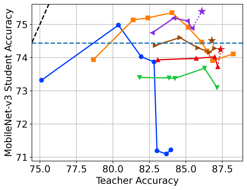
(a) MobileNetV3

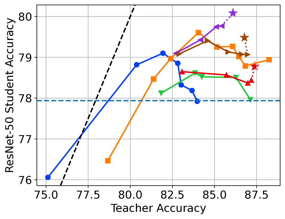
(b) ResNet50

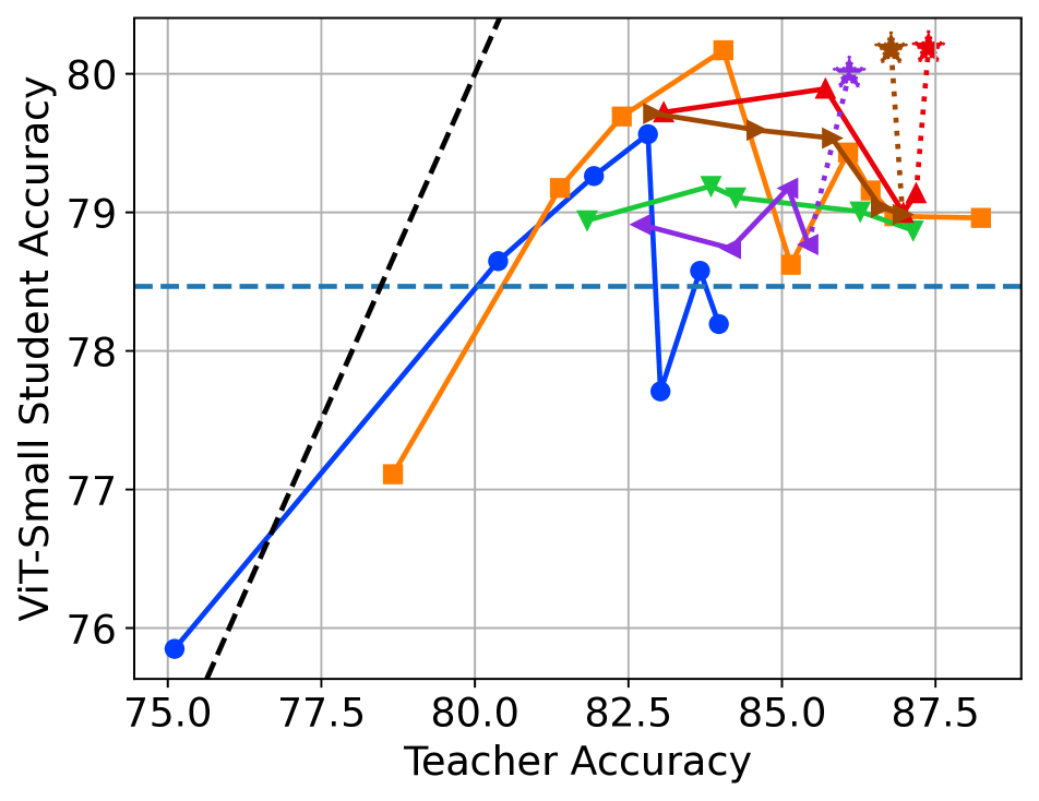
(c) ViT-Small

Figure 7: Knowledge distillation accuracy of representative student architectures (ResNet-50, ViT-Small, MobileNetV3) for pretrained teachers from Timm library. We train for 150 epochs and Fig. 3 shows results for 300 epoch training.

Teacher Name	Teacher Accuracy	Student Top-1 Accuracy
		ResNet-50		ViT-Small		MobileNetv3-Large
		300	150	300	150	300	150
beit_large_patch16_512	$88.58$	$41.76$	$41.45$	$37.03$	$35.87$	—	—
convnext_tiny_in22ft1k	$82.90$	$80.13$	$79.08$	$80.82$	$79.71$	$75.41$	$74.37$
convnext_large + convnext_base + convnext_small + convnext_tiny + convnext_nano	$84.34$	$80.34$	$78.94$	$80.73$	$79.82$	—	—
convnext_small_in22ft1k	$84.59$	$80.63$	$79.41$	$81.16$	$79.59$	$75.70$	$74.60$
convnext_base_in22ft1k	$85.81$	$80.56$	$79.13$	$81.36$	$79.54$	$75.44$	$74.30$
convnext_large_in22ft1k	$86.61$	$80.17$	$79.07$	$80.77$	$79.04$	$75.35$	$74.16$
convnext_xlarge_in22ft1k + convnext_large_in22ft1k + convnext_base_in22ft1k + convnext_small_in22ft1k + convnext_tiny_in22ft1k	$86.78$	$80.78$	$79.48$	$81.67$	$80.18$	$75.82$	$74.51$
convnext_xlarge_in22ft1k	$86.96$	$80.07$	$79.07$	$80.69$	$78.98$	$75.26$	$74.28$
convnext_xlarge_384_in22ft1k	$87.53$	$79.67$	$78.50$	$79.92$	$78.38$	—	—
deit3_small_patch16_224_in21ft1k	$83.07$	$79.60$	$78.65$	$81.23$	$79.72$	$75.04$	$73.93$
deit3_huge_patch14_224 + deit3_large_patch16_224 + deit3_base_patch16_224 + deit3_small_patch16_224	$85.30$	$79.69$	$78.82$	$80.25$	$79.55$	—	—
deit3_base_patch16_224_in21ft1k	$85.71$	$79.98$	$78.57$	$81.24$	$79.89$	$75.16$	$73.98$
deit3_large_patch16_224_in21ft1k	$86.98$	$79.61$	$78.37$	$80.81$	$79.00$	$75.08$	$74.02$
deit3_huge_patch14_224_in21ft1k	$87.18$	$79.52$	$78.44$	$80.59$	$79.14$	$74.79$	$73.73$
deit3_huge_patch14_224_in21ft1k + deit3_large_patch16_224_in21ft1k + deit3_base_patch16_224_in21ft1k + deit3_small_patch16_224_in21ft1k	$87.39$	$80.25$	$78.78$	$81.26$	$80.19$	$75.28$	$74.24$
deit3_large_patch16_384_in21ft1k	$87.73$	$79.06$	$78.00$	$79.71$	$78.80$	—	—
ig_resnext101_32x8d	$82.70$	$80.32$	$79.10$	$80.30$	$78.91$	$76.03$	$74.75$
ig_resnext101_32x16d	$84.17$	$80.78$	$79.43$	$80.93$	$78.74$	$76.37$	$75.19$
ig_resnext101_32x32d	$85.10$	$81.04$	$79.75$	$81.03$	$79.17$	$76.42$	$75.11$
ig_resnext101_32x48d	$85.43$	$80.93$	$79.77$	$80.67$	$78.77$	$76.01$	$74.88$
ig_resnext101_32x48d + ig_resnext101_32x32d + ig_resnext101_32x16d + ig_resnext101_32x8d	$86.10$	$81.30$	$80.08$	$82.01$	$80.00$	$76.70$	$75.39$
ig_resnext101_32x48d + convnext_xlarge_in22ft1k + volo_d5_224 + deit3_huge_patch14_224	$87.39$	$80.71$	$79.63$	$81.65$	$80.00$	—	—
resnet18	$69.74$	$71.29$	$71.29$	$71.29$	$71.18$	—	—
resnet34	$75.11$	$76.46$	$76.06$	$76.36$	$75.85$	$73.90$	$73.32$
resnet50	$80.38$	$79.83$	$78.82$	$79.81$	$78.65$	$75.63$	$74.98$
resnet101	$81.94$	$80.07$	$79.10$	$80.82$	$79.26$	$74.92$	$74.03$
resnet152	$82.82$	$79.88$	$78.85$	$79.72$	$79.56$	$74.82$	$73.87$
resnet101d	$83.02$	$79.75$	$78.32$	$78.92$	$77.71$	$72.78$	$71.19$
resnet152d	$83.67$	$79.62$	$78.19$	$78.77$	$78.58$	$73.05$	$71.10$
resnet200d	$83.97$	$79.40$	$77.92$	$80.18$	$78.19$	$73.10$	$71.22$
resnetv2_152x2_bitm	$84.46$	$79.57$	$78.63$	$80.04$	$78.52$	$75.12$	$73.87$
resnetv2_152x4_bitm	$84.94$	—	$78.09$	—	$78.97$	—	$73.69$
swinv2_cr_tiny_ns_224	$81.79$	$79.41$	$78.47$	$80.56$	$79.29$	$74.23$	$73.43$
swinv2_tiny_window8_256	$81.83$	$79.30$	$78.12$	$80.32$	$78.94$	$74.46$	$73.40$
swinv2_tiny_window16_256	$82.82$	$79.43$	$78.31$	$80.59$	$79.30$	$74.31$	$73.57$
swinv2_cr_small_224	$83.12$	$79.15$	$78.33$	$79.78$	$78.64$	$74.59$	$73.42$
swinv2_cr_small_ns_224	$83.48$	$79.43$	$78.62$	$80.38$	$78.94$	$74.56$	$73.62$
swinv2_small_window8_256	$83.84$	$79.66$	$78.61$	$80.35$	$79.19$	$74.44$	$73.39$
swinv2_small_window16_256	$84.22$	$79.21$	$78.41$	$80.00$	$78.30$	$74.84$	$73.45$
swinv2_base_window8_256	$84.25$	$79.57$	$78.52$	$80.32$	$79.11$	$74.73$	$73.37$
swinv2_base_window16_256	$84.59$	$78.94$	$78.30$	$79.50$	$78.32$	$74.50$	$73.63$
swinv2_base_window12to16_192to256_22kft1k	$86.27$	$79.76$	$78.51$	$80.80$	$79.01$	$74.35$	$73.68$
swinv2_large_window12to16_192to256_22kft1k	$86.94$	$79.31$	$78.38$	$79.86$	$78.43$	$74.39$	$73.51$
swinv2_base_window12to24_192to384_22kft1k	$87.14$	$79.18$	$77.96$	$80.01$	$78.87$	—	$73.10$
swinv2_large_window12to24_192to384_22kft1k	$87.47$	$78.48$	$77.65$	$78.33$	$78.38$	—	$73.07$
tf_efficientnet_b0	$76.85$	—	$75.10$	—	$75.97$	$73.68$	$72.93$
tf_efficientnet_b0_ns	$78.67$	$77.27$	$76.47$	$77.96$	$77.11$	$74.94$	$73.94$
tf_efficientnet_b1	$78.83$	—	$77.45$	—	$77.97$	$75.48$	$74.69$
tf_efficientnet_b2	$80.08$	—	$78.17$	—	$78.88$	$75.97$	$75.01$
tf_efficientnet_b1_ns	$81.38$	$79.52$	$78.47$	$80.38$	$79.18$	$76.14$	$75.14$
tf_efficientnet_b3	$81.65$	—	$78.88$	—	$79.56$	$76.39$	$75.38$
tf_efficientnet_b2_ns	$82.39$	$80.17$	$78.97$	$80.94$	$79.69$	$76.43$	$75.20$
tf_efficientnet_b4	$83.03$	—	$78.91$	—	$78.56$	$75.64$	$74.65$
tf_efficientnet_b5	$83.81$	—	$79.20$	—	$79.18$	$76.01$	$75.06$
tf_efficientnet_b3_ns	$84.05$	$80.71$	$79.60$	$81.72$	$80.17$	$76.44$	$75.35$
tf_efficientnet_b6	$84.11$	—	$78.92$	—	$79.21$	$75.58$	$74.41$
tf_efficientnet_b7	$84.93$	—	$79.16$	—	$79.24$	$75.42$	$74.43$
tf_efficientnet_b4_ns	$85.14$	$80.83$	$79.25$	$81.51$	$78.62$	$75.81$	$74.92$
tf_efficientnet_b8	$85.35$	—	$78.84$	—	$78.17$	$75.15$	$73.86$
tf_efficientnet_b5_ns	$86.08$	$80.71$	$79.27$	$81.05$	$79.43$	$75.57$	$74.47$
tf_efficientnetv2_xl_in21ft1k	$86.41$	$11.58$	$12.46$	$8.40$	$7.69$	—	—
tf_efficientnet_b6_ns	$86.44$	$80.21$	$79.02$	$80.91$	$79.16$	$75.36$	$74.20$
tf_efficientnet_b7_ns	$86.83$	$80.34$	$78.79$	$80.89$	$78.97$	$74.93$	$73.91$
tf_efficientnet_l2_ns_475	$88.24$	—	$78.94$	—	$78.96$	—	$74.11$
vit_large_patch16_384	$87.09$	$79.63$	$78.45$	$80.48$	$78.88$	—	—
volo_d5_224 + volo_d4_224 + volo_d3_224 + volo_d2_224 + volo_d1_224	$86.09$	$80.45$	$79.31$	$80.81$	$79.16$	—	—
volo_d5_512	$87.04$	—	$78.04$	—	$76.61$	—	—

Table 13: Effect of distillation from pretrained teachers (Timm library) on the performance of MobileNetV3-large, ResNet-50, ViT-Small trained for $150$ and $300$ epochs. This table includes the details of Figs. 7 and 3.

B.2 Super ensembles on ImageNet

It is common to limit the number of models in an ensemble to less than 10 members and typically only $4$. The reason is partly that larger ensembles are more expensive to evaluate at test time as well as training with knowledge distillation. Dataset reinforcement allows us to consider expensive teachers such as super ensembles with significantly more than 10 members. In Tab. 15 we present results for super ensembles on CIFAR-100 and in Fig. 8 we present results on ImageNet. On CIFAR-100 we create super ensembles by training 128 models in parallel for ResNet-18, ResNet-50, and ResNet-152 architectures. To increase diversity, we train models with 16 choices of enable/disable 4 augmentations (CutMix, MixUp, RandAugment, and Label Smoothing) and train with $8$ different random seeds for each choice. In total we train $8\times 16=128$ models. Tab. 15 shows the accuracy of the super ensembles while Tab. 15 shows the accuracy of distillation with the super ensembles. We observe that the best student accuracy is achieved with the largest ensemble 128xR152. Interestingly, super ensembles of small models (128xR50) are better than standard ensembles of large models (10xR152). With super ensembles we achieve strong accuracies for ResNet-50 at 86.30 and ResNet-152 at 87.03.

We also consider super ensembles for ImageNet using dataset reinforcement. Knowledge distillation with super ensembles of larger than 10 members on ImageNet becomes challenging and resource demanding. Fig. 8 shows the validation accuracy of the ensemble and Fig. 9 shows the accuracy of student training with the reinforced ImageNet dataset using the super ensemble. We observe that the entropy and confidence of the teacher on the validation set are not more correlated with the distillation accuracy than the accuracy of the validation teacher. In particular, large ensembles are more accurate but not necessarily better teachers. In summary, we observe that the optimal ensemble size for KD is around 4.

	10xR18	128xR18	10xR50	128xR50	10x152	128xR152
ResNet-18	83.57	84.24	83.43	84.07	83.65	84.25
ResNet-50	84.40	85.16	84.33	86.38	86.03	86.30
ResNet-152	85.01	85.74	85.00	86.80	86.85	87.03

Table 14: Distillation on CIFAR-100 with super diverse ensembles.

	Single best	Ensemble (128x)
ResNet-18	81.57	85.88
ResNet-50	83.43	87.29
ResNet-152	84.44	87.92

Table 15: Accuracy of super diverse ensembles on CIFAR-100.

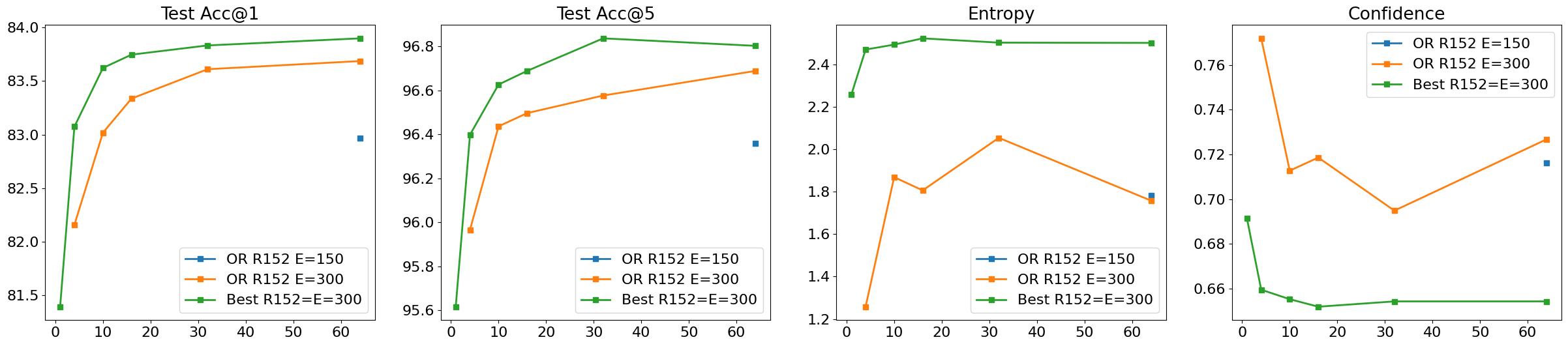
Figure 8: ImageNet accuracy of super ensembles as the size of the ensemble is increased. OR means the ensemble is created from diverse augmentation choices while Best means only the random seed is different between models.

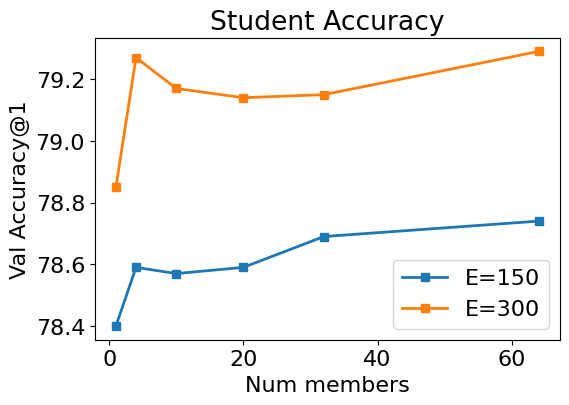
Figure 9: ImageNet super ensemble distillation accuracy for ResNet-50 facilitated by dataset reinforcement.

Appendix C Expanded study on reinforcing ImageNet

In this section, we provide ablations on the number and type of augmentations using a single relatively cheap teacher (ConvNext-Base-IN22FT1K) that still provides comparatively good improvements across all students.

C.1 What is the best combination of augmentations for reinforcement?

To recap, using our selected teachers from Sec. 2.1, we investigate the choice of augmentations for dataset reinforcement. Utilizing Fast Knowledge Distillation [55], we store the sparse outputs of a teacher on multiple augmentations. For efficiency, we store top 10 probabilities predicted by the teacher, along with the augmentation parameters and reapply augmented images in the data loader of the student. We observe that light-weight CNNs perform best on easier reinforcements while transformers perform best with difficult reinforcements. We balance this tradeoff using a mid-difficulty reinforcement.

We refer to the combination of baseline augmentations fixed resize, random crop and horizontal flip by CropFlip. In addition, we consider the following augmentations for dataset reinforcement: Random-Resize-Crop (RRC), MixUp [72] and CutMix [70] (Mixing), and RandomAugment [14] and RandomErase (RA/RE). We also combine Mixing with RA/RE and refer to it as M^∗$+$R^∗. We add all augmentations on top of RRC and for clarity add + as shorthand for RRC$+$. Except for mixing augmentations, reapplying all augmentations has zero overhead compared to standard training with the same augmentations. For mixing augmentations, our current implementation has approximately $30\%$ wall-clock time overhead because of the extra load time of mixing pairs stored with each reinforced sample. We discuss efficient alternatives in Sec. C.3. Our balanced solution, RRC$+$RA/RE, does not use mixing and has zero overhead.

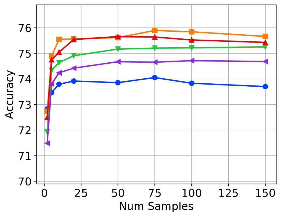
(a) Light-weight CNN (MobileNetV3)

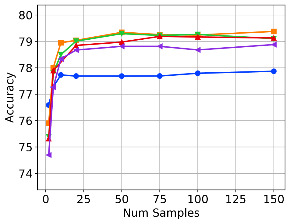
(b) Heavy-weight CNN (ResNet-50)

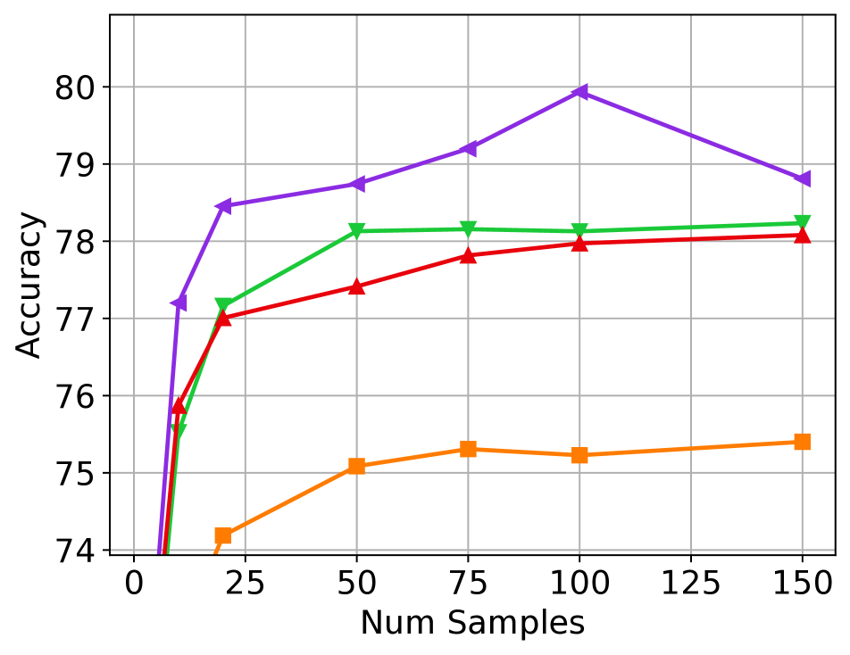
(c) Transformer (ViT-Small)

Figure 10: Light-weight CNNs prefer easy while Transformers prefer difficult reinforcements and we balance the tradeoff. ImageNet validation accuracy of three representative architectures trained on reinforcements of ImageNet. We use ConvNext-Base-IN22FT1K as the teacher and train for 150 epochs. The x-axis is the number of augmentations stored per original sample in the ImageNet training set. In favor of dataset reinforcement, we observe that training with $25-50$ samples provides similar gains to training with more samples. The baseline augmentation is Fixed Resize-RandomCrop and horizontal flip (CropFlip). In addition we consider the following augmentations for reinforcement: Random-Resize-Crop and horizontal flip (RRC), MixUp and CutMix (Mixing), RandomAugment/RandomErase (RA/RE) and Mixing+RA/RE (M^∗$+$R^∗). We add these augmentations on top of RRC and for clarity add + as shorthand for RRC$+$.

Figure 10 shows the accuracy of various models trained on reinforced datasets. We observe that the light-weight CNN performs best with RRC as the most simple augmentation after CropFlip while the transformer performs best with the most difficult set of reinforcements in RRC$+$M^∗ $+$R^∗. This observation matches the standard state-of-the-art recipes for training these models. At the same time, we observe that RRC$+$RA/RE provides nearly the best performance for all models without the extra overhead of mixing methods in our implementation.

Consistent across three models and reinforcements, we observe that even though we train for 150 epochs, at most $25-50$ different augmentations of each training sample is enough to achieve the best accuracy for almost all methods. This gives at least $\times 3$ reduction in the number of samples we can take advantage of given a fixed training budget. Based on this observation and following [6], in Sec. 3 we train models for up to 1000 epochs while reinforce datasets with 400 augmentation samples.

C.2 Augmentation: invariance vs imitation

Data augmentation is crucial to train generalizable models in various domains. The key objective is to make the model invariant to content-preserving transformations. In knowledge distillation, however, it is not clear whether the student benefits more from being invariant to data augmentations as in Eq. 2 or from imitating teacher’s variations on augmented data as in Eq. 3. The training objective for each case is as follows:

$$\text{(Invariance)}\hskip 14.22636pt\min_{\theta}\,\mathbb{E}_{{\bm{x}}\sim\mathcal{D},\hat{{\bm{x}}}\sim\mathcal{A}({\bm{x}})}\mathcal{L}(f_{\theta}(\hat{{\bm{x}}}),g({\color[rgb]{0,0,1}{\bm{x}}}))$$ (2)

$$\text{(Imitation)}\hskip 14.22636pt\min_{\theta}\,\mathbb{E}_{{\bm{x}}\sim\mathcal{D},\hat{{\bm{x}}}\sim\mathcal{A}({\bm{x}})}\mathcal{L}(f_{\theta}(\hat{{\bm{x}}}),g({\color[rgb]{0,0,1}\hat{{\bm{x}}}}))$$ (3)

where, $\mathcal{D}$ is the training dataset, $\mathcal{A}$ is augmentation function, $f_{\theta}$ is the student model parameterized with $\theta$, $g$ is the teacher model, and $\mathcal{L}$ is the loss function between student and teacher outputs.

In Fig. 11, we compare the above training objectives for a wide range of augmentations in computer vision. For most augmentations, we observe imitation is more effective than invariance. This is consistent with observation in [6]. Therefore, in our setup we use augmentations only for imitation (and not invariance).

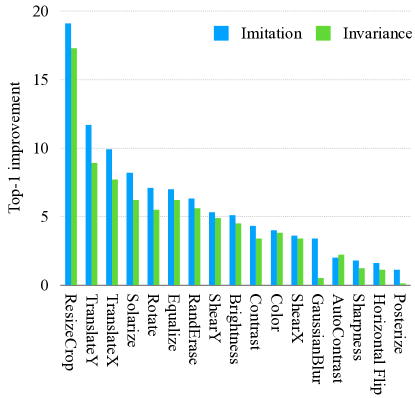
Figure 11: ImageNet top-1% accuracy improvement when distilling knowledge from a ConvNext (Base-IN22FT1K) teacher to a ViT-tiny student using a single augmentation with training objectives in Eq. 2 and Eq. 3. No augmentation top-1% accuracy is $54\%$.

C.3 Library size: Can we limit the mixing pairs?

Mixing augmentations have the extra overhead of the load time for the corresponding pair in each mini-batch. Standard training does not have such an overhead because the mixing is performed on random pairs within a mini-batch. In dataset reinforcement, the pairs that have been matched in the reinforcement phase are limited to the number of samples stored and do not always appear in the same mini-batch during the student training time. This means, we have to load the matching pair for every sample in the mini-batch that doubles the data load time and becomes an overhead for CPU-bound models. This overhead in the smallest models we consider is at most 30%. Even though much lower than the cost of knowledge distillation, it is still more than our desiderata would allow.

We consider an alternative where the pairing is done only with a library of selected samples from the training set. The library can be loaded in the memory once and reduce the additional cost incurred during the training. Fig. 12 shows the performance as we vary the library size. Even a relatively large library does not cover the accuracy drop caused by the reduced randomness in the mixing. The reason is that to reduce the cost, we can only have one augmentation per sample in the library which reduces the randomness from the mixing substantially and negatively affects knowledge distillation.

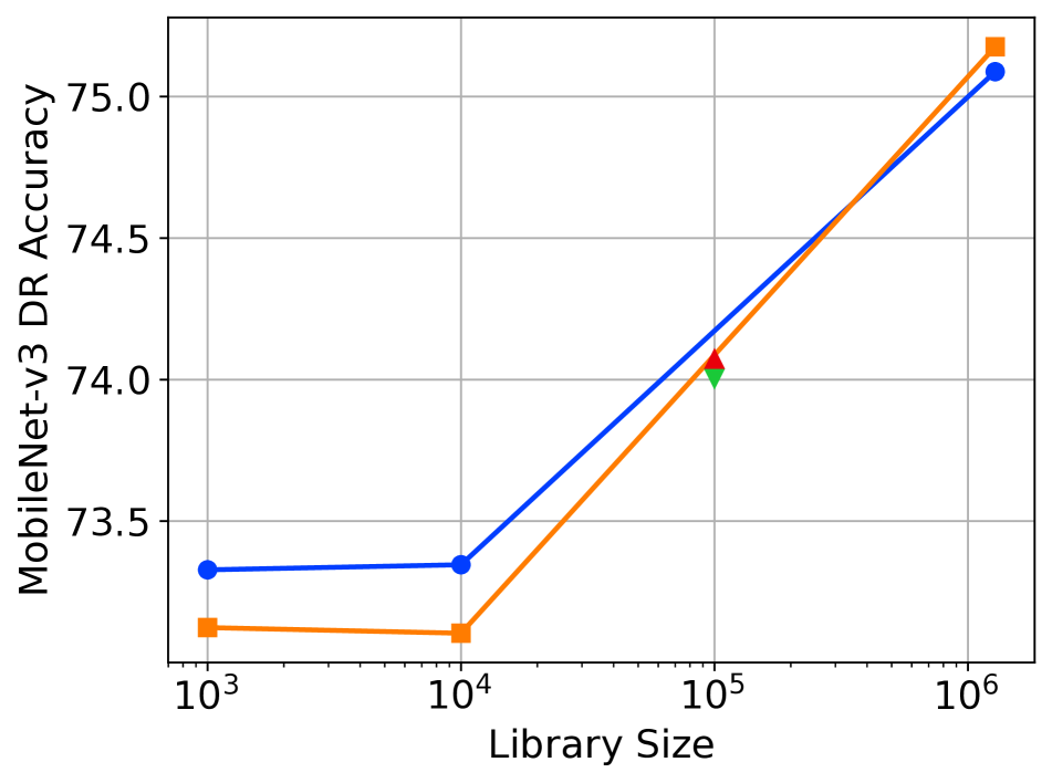
(a) MobileNetV3

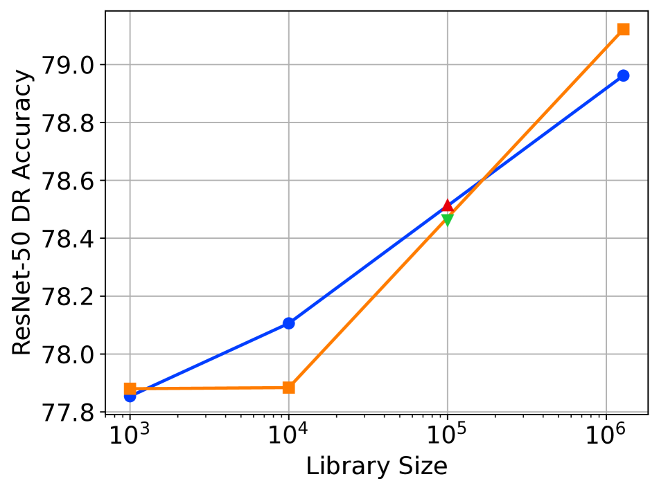
(b) ResNet50

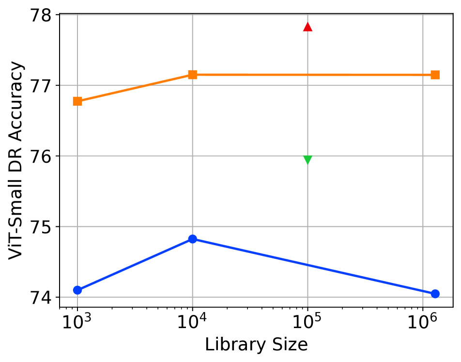
(c) ViT-Small

Figure 12: Library of mixing pairs reduces wall-clock overhead for mixing methods but negatively impacts accuracy. We plot the validation accuracy for models trained with ImageNet⁺ as we vary the library size. The teacher is ConvNext-Base-IN22FT1K. See Sec. C.3 for details. (E=150)

We also consider variations of mixing in Fig. 13. We consider two variations: Double-mix and Self-mix. In double-mix, for every augmented pair, we store two outputs with two sets of mixing coefficients. This means for every mini-batch we can load half the mini-batch along with a random pair for each sample, perform the stored augmentation on each and get two different mixed samples. As a result the overhead is zero. Second alternative, self-mix, mixes every image only by itself. As such, there is no data load time, but there is still an extra overhead of preprocessing the input twice. Fig. 13 shows that neither of the considered alternatives provide a better tradeoff compared with RRC$+$RA/RE. Therefore, we use RRC$+$RA/RE in our paper and call it ImageNet⁺.

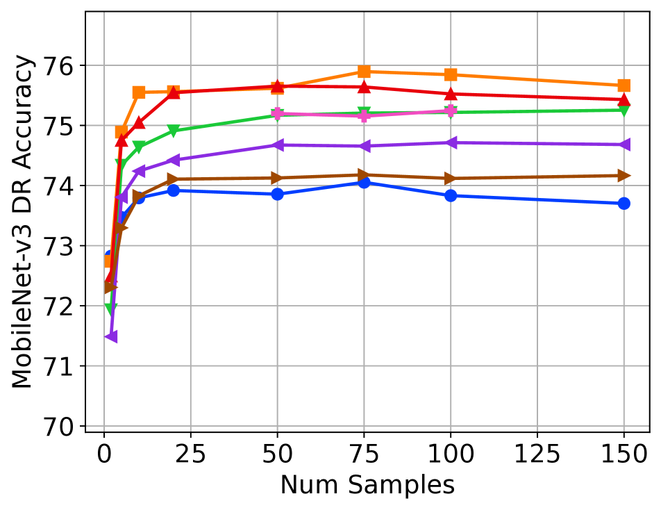
(a) Light-weight CNN (MobileNetV3)

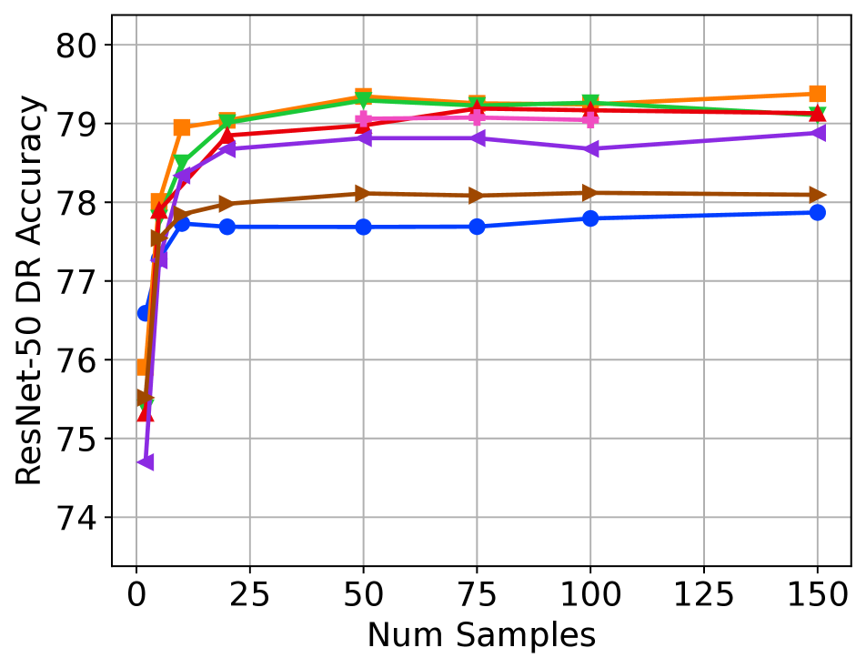
(b) Heavy-weight CNN (ResNet-50)

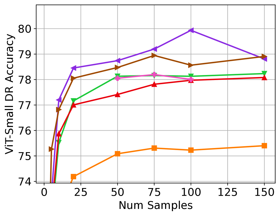
(c) Transformer (ViT-Small)

Figure 13: Alternative Mixing Augmentations. Accuracy of three representative architectures trained on reinforcements of ImageNet. We use ConvNext-Base-IN22FT1K as the teacher and train for 150 epochs. The x-axis is the number of augmentations stored per original sample in the ImageNet training set. Augmentations used are Fixed Resize-RandomCrop and horizontal flip (CropFlip), Random-Resize-Crop and horizontal flip (RRC), MixUp and CutMix (Mixing), RandomAugment/RandomErase (RA/RE) and Mixing+RA/RE (M*+R*). Alterantive mixing augmentations: Double-mix (Dmix) and Self-mix (Smix).

C.4 What is the best curriculum of reinforcements?

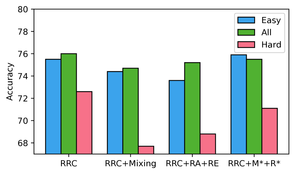
(a) Light-weight CNN (MobileNetV3)

(b) Heavy-weight CNN (ResNet-50)

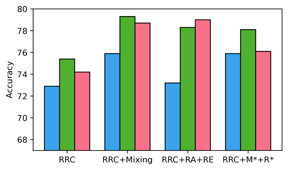
(c) Transformer (ViT-Small)

Figure 14: Tradeoff in augmentation difficulty can be further reduced with curriculums. Using random samples of the optimal augmentation is the best (‘All’). If we have access to one reinforcement dataset or we want to only keep a subset of data for efficiency, then it is better to use ‘easy’ curriculums for CNN based architectures and ‘hard’ curriculums for Transformers. Full table in Sec. C.5.

The one-time cost of reinforcing a dataset allows us to generate as much useful information as we need and store it for future use. An example is various metrics that can be used to devise learning curriculums that adapt to specific students. In this section we consider a set of initial curriculums we get for free with our dataset reinforcement strategy. Specifically, the output of the teacher on each sample also incorporates the confidence of the teacher on its prediction. We can use the confidence or the entropy of its predictions to make curriculums.

Given ${\bm{p}}\in{\mathbb{R}}^{c}$ the set of predicted probabilities of the teacher for $c$ classes, we define confidence as $\max{\bm{p}}_{j}$. For every sample, we order its augmentations by the confidence value from $0$ to #samples. During training, at each iteration we only sample from a range of augmentations with indices between $[a,b]$, where $0\leq a,b<\text{\#samples}$. We devise curriculums by smoothly changing $a,b$ during the training using a cosine function between specified values of initial and final values for $a,b$.

Fig. 14 shows the performance of various Easy, Hard, and All curriculums. Easy curriculums start from $[0,10]$ (the $10\%$ easiest samples), hard samples start from $[90,100]$ (the $10\%$ hardest samples), and All curriculums start from $[0,100]$ (all the samples). We observe that the curriculum provides an alternative knob to control the difficulty of reinforcements that we can use adaptively during the training of the student. For example, the best performance of the light-weight CNN is with RRC combined with the All curriculum, but similar performance can be achieved with RRC$+$RA/RE combined with an Easy curriculum. Similarly, the transformer achieves its best performance with RRC$+$M^∗ $+$R^∗ combined with the All curriculum, while a similar performance can be achieved with RRC$+$Mixing and a Hard curriculum.

In Sec. C.6, we study various objectives for choosing most useful samples during the reinforcement process. We consider storing on the most informative samples according to a number of metrics such as entropy, loss, and clustering. We make similar observations to the behaviour of curriculums that the objectives that increase hardness benefit the transformer while the easy objectives benefit the light-weight CNN.

C.5 Additional details of curriculums

We study reinforcements on curriculums shown in Fig. 15. Table 16 provides the full results for the effect of dataset reinforcement curriculums. We summarized these results in Fig. 14 where we compared ‘*$\rightarrow$all’ curriculums that end with ‘all’ of the data. We observe that the beginning of the curriculum has much more impact on the generalization than the end of the curriculum. We observe that ‘all$\rightarrow$*’ curriculums perform the best while ‘hard$\rightarrow$*’ curriculums perform near optimal for ViT-Small and ‘easy$\rightarrow$*’ performs best for MobileNetV3-Large. At the same time, we observe clearly that the hard and easy curriculums result in significantly worse generalization when used to train the opposite architecture, i.e., ‘easy$\rightarrow$*’ for ViT-Small and ‘hard$\rightarrow$*’ for MobileNetV3-Large. This result clearly demonstrates the tradeoff in the architecture independent generalization controlled by the difficulty of reinforcements.

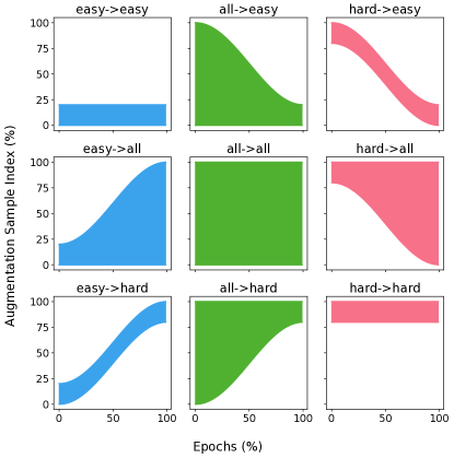
Figure 15: Illustration of curriculums. The x-axis shows the percentage of training epochs while the y-axis shows the index of augmentation samples in percentages as we order them from easy to hard by the confidence of the teacher. Highlighted regions show the subset of indices of reinforcements to uniformly draw from at each epoch.

Curriculum

MobileNetV3-Large

ResNet50

ViT-Small

RRC

+RA/RE

+Mixing

+M*+R*

RRC

+RA/RE

+Mixing

+M*+R*

RRC

+RA/RE

+Mixing

+M*+R*

easy->all

${75.5}$

${\bm{75.9}}$

${73.6}$

${74.4}$

${79.0}$

${79.0}$

${77.8}$

${78.1}$

${72.9}$

${75.9}$

${73.2}$

${75.9}$

easy->easy

${75.2}$

${75.7}$

${74.3}$

${74.5}$

${79.0}$

${79.2}$

${77.7}$

${78.0}$

${72.6}$

${75.9}$

${73.1}$

${75.9}$

easy->hard

${75.6}$

${\bm{75.8}}$

${74.1}$

${74.6}$

${79.0}$

${79.2}$

${77.8}$

${78.0}$

${72.6}$

${76.2}$

${72.9}$

${76.0}$

all->all

${\bm{76.0}}$

${75.5}$

${75.2}$

${74.7}$

${\bm{79.4}}$

${79.0}$

${\bm{79.3}}$

${78.7}$

${75.4}$

${78.1}$

${78.3}$

${\bm{79.3}}$

all->easy

${75.7}$

${75.5}$

${75.2}$

${74.6}$

${\bm{79.5}}$

${79.2}$

${\bm{79.3}}$

${78.9}$

${75.2}$

${78.4}$

${78.2}$

${\bm{79.2}}$

all->hard

${\bm{75.8}}$

${75.5}$

${75.3}$

${74.6}$

${\bm{79.4}}$

${\bm{79.3}}$

${79.2}$

${78.9}$

${75.3}$

${77.8}$

${78.5}$

${\bm{79.3}}$

hard->all

${72.6}$

${71.1}$

${68.8}$

${67.7}$

${76.7}$

${75.6}$

${76.7}$

${75.5}$

${74.2}$

${76.1}$

${79.0}$

${78.7}$

hard->easy

${72.5}$

${71.3}$

${68.7}$

${67.7}$

${76.7}$

${75.9}$

${77.0}$

${75.3}$

${74.2}$

${76.2}$

${78.8}$

${78.6}$

hard->hard

${72.2}$

${71.4}$

${68.9}$

${67.7}$

${76.8}$

${75.7}$

${76.9}$

${75.7}$

${73.9}$

${76.2}$

${79.0}$

${78.6}$

Table 16: The effect of curriculum. We observe that the beginning of the curriculum has much more impact on the generalization than the end of the curriculum (accuracy within the groups of three rows is similar). Accuracies within 0.2% of the best accuracy in each column are highlighted.

C.6 Optimal augmentation sample selection

We discussed that augmentations used to reinforce the dataset are sampled from a pool of augmentation operations and that we apply the augmentations with a predetermined application probability. The setup of dataset reinforcement allows us to optimize for the most informative augmentation samples. For example, we can generate a large set of candidate augmentations and choose a subset with maximum or minimum values of ad-hoc metrics. We considered selecting samples according to metrics such as confidence, entropy, and loss. Given ${\bm{p}}\in{\mathbb{R}}^{c}$, the set of predicted probabilities of the teacher for $c$ classes, we define confidence as $\max{\bm{p}}_{j}$, the entropy as $-\sum_{j}{\bm{p}}_{j}\log{\bm{p}}_{j}$, and the loss as $-\log{\bm{p}}_{y}$ where $y$ is the ground-truth label. To encourage diversity, we also considered selecting samples based on the clustering of the predicted probability vectors by performing KMeans on ${\bm{p}}$ vectors of the candidates and selecting one sample per cluster. Figure 16 shows the performance of a subset of sample selection methods we considered.

Generally we observe that max-entropy/min-confidence objectives demonstrate similar behaviors better than min-entropy/max-confidence. So we only show the min-confidence variant. We observe that overall random samples (blue lines) provides the best validation accuracy if used with the right augmentations (RRC$+$RA/RE for light-weight CNNs and RRC$+$M^∗ $+$R^∗ for transformers). Using min-confidence (orange) with RRC$+$M^∗ $+$R^∗ (dashed orange), leads to similar generalization on transformers while hurting the generalization on CNNs. This matches our observations with the complexity of augmentations and curriculums that transformers prefer difficult samples. We observe that diversified samples using KMeans clustering (green) provide similar behavior to random samples (blue) while for transformers provide more consistent improvements at varying number of samples (dashed green compared with dashed blue). We identify this potential for future work and investigate reinforced datasets with random samples in the rest of the paper. Note that the curriculums are a generalization of the objective-based metrics that are adaptive to the student (See Sec. C.4 and Sec. C.5).

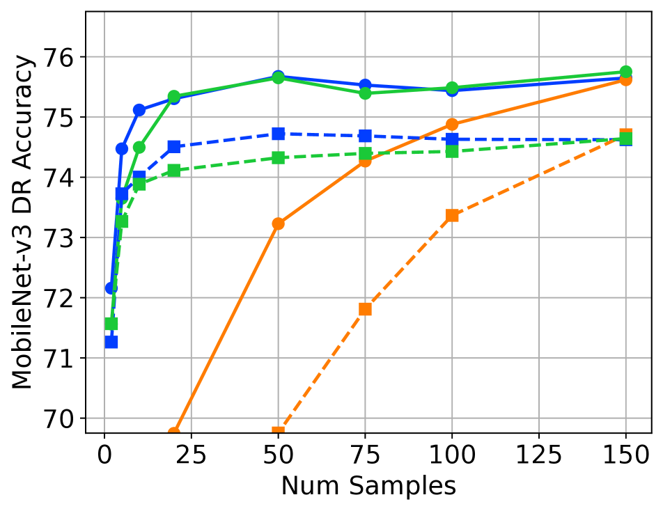
(a) MobileNetV3

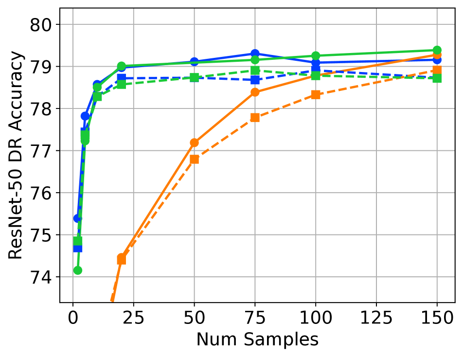
(b) ResNet50

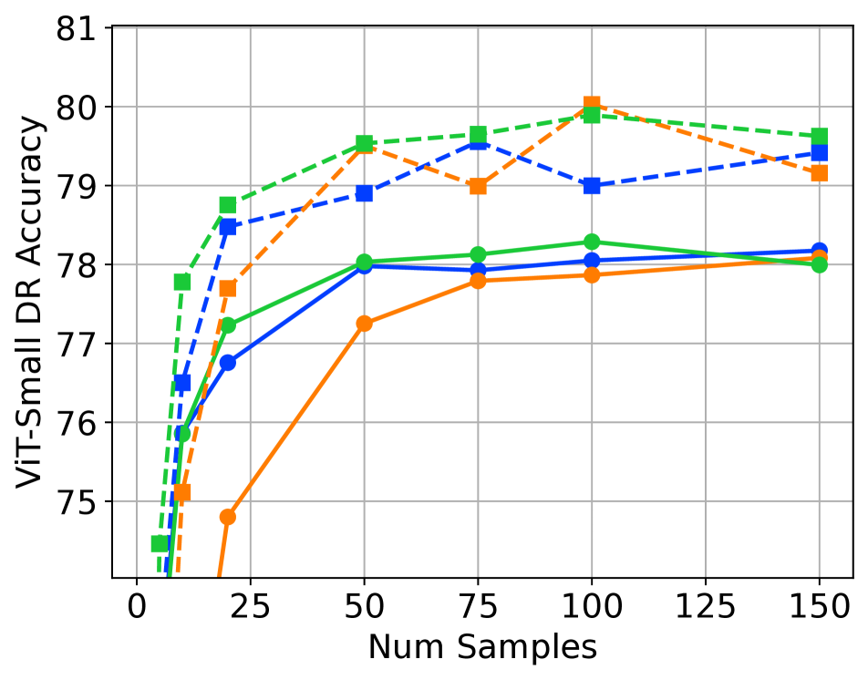
(c) ViT-Small

Figure 16: Optimal augmentation sample selection. ImageNet⁺ accuracy for varying objectives and number of samples. The teacher is ConvNext (Base-IN22FT1K) (E=150)

Appendix D Additional pretraining/finetuning/transfer learning results

In Tab. 17 we provide results for various combinations of pretraining and fine-tuning on reinforced/non-reinforced datasets. We observe that the best results are achieved when both pretraining and fine-tuning are done using reinforced datasets. We also observe that the improvement is significant compared to when only one of the pretraining/fine-tuning datasets is reinforced. The idea of training and fine-tuning on multiple reinforced datasets is unique to dataset reinforcement and would be challenging to replicate with standard data augmentations or knowledge distillation.

We train models for 100, 400, 1000 epochs on CIFAR-100, Food-101 and 1000, 4000, and 10000 epochs on Flowers-102 and report the best accuracy for each model. Models pretrained/fine-tuned on non-reinforced datasets tend to overfit at longer training while models trained on reinforced datasets benefit from longer training.

For future tasks and datasets, additional task-specific information could be considered as reinforcements. For example, an object detection dataset can be further reinforced using the teacher’s uncertainty on bounding boxes, occlusion estimate, and border uncertainty. Multi-modal models such as CLIP are an immediate future work that can provide variety of additional training signal based on the relation to an anchor text.

Model	Pretraining dataset	Fine-tuning dataset
		CIFAR-100	CIFAR-100+	Flowers-102	Flowers-102+	Food-101	Food-101+
MobileNetV3-Large	None	80.2	83.6	68.8	87.5	85.1	88.2
	ImageNet	84.4	87.2	92.5	94.1	86.1	89.2
	ImageNet+ (Ours)	86.0	87.5	93.7	95.3	86.6	89.5
ResNet-50	None	83.8	85.0	87.3	85.0	89.1	90.2
	ImageNet	88.4	89.5	93.6	94.9	90.0	91.8
	ImageNet+ (Ours)	88.8	89.8	95.0	96.3	90.5	92.1
SwinTransformer-Tiny	None	35.0	82.2	78.3	72.5	89.6	90.9
	ImageNet	90.6	90.7	96.3	96.5	92.3	92.7
	ImageNet+ (Ours)	90.9	91.2	96.6	97.0	93.0	92.9

Table 17: Pretraining/Finetuning/Transfer learning for fine-grained object classification.

Appendix E Full table of calibration results

In Tab. 18 we provide the full results for Fig. 5. We see observe that validation ECE of ImageNet⁺ pretrained models is lower than ImageNet pretrained models.

Model	Method	Epochs	Train ECE	Val ECE	ECE gap	Train Error	Val Error	Error gap
MobileNetV3-Large	ImageNet	300	0.1503	0.0727	0.0776	0.0934	0.2509	0.1575
	ImageNet+	300	0.0339	0.0309	0.0030	0.1400	0.2298	0.0898
	ImageNet	1000	0.1489	0.0608	0.0881	0.0599	0.2491	0.1891
	ImageNet+	1000	0.0312	0.0323	0.0011	0.1218	0.2206	0.0988
	KD	300	0.0303	0.0297	0.0006	0.1550	0.2358	0.0808
ResNet-50	ImageNet	300	0.1938	0.1513	0.0425	0.1239	0.2122	0.0883
	ImageNet+	300	0.0263	0.0362	0.0098	0.1115	0.1944	0.0829
	ImageNet	1000	0.1887	0.1348	0.0539	0.0906	0.2036	0.1130
	ImageNet+	1000	0.0241	0.0360	0.0119	0.0936	0.1830	0.0894
	KD	300	0.0250	0.0339	0.0089	0.1065	0.1846	0.0781
SwinTransformer-Tiny	ImageNet	300	0.1084	0.0663	0.0421	0.0734	0.1910	0.1176
	ImageNet+	300	0.0201	0.0381	0.0180	0.0818	0.1698	0.0880
	ImageNet	1000	0.1042	0.0522	0.0519	0.0421	0.1905	0.1484
	ImageNet+	1000	0.0195	0.0397	0.0203	0.0743	0.1621	0.0877
	KD	300	0.0206	0.0379	0.0173	0.0958	0.1701	0.0742

Table 18: Full calibration error and validation error for Fig. 5.

Appendix F Cost of dataset reinforcement

In Sec. C.1, we observe that similar accuracy to knowledge distillation is reached with $\times 3$ fewer samples than the number of target epochs. This reduces the reinforcement cost. ImageNet⁺ took 2080 mins to generate using 64xA100 GPUs which is highly parallelizable and similar to training ResNet-50 for 300 epochs on 8xA100 GPUs. The parallelization is another significant advantage to knowledge distillation because samples are reinforced independently while knowledge distillation requires following a trajectory on training samples. For CIFAR-100, Flowers-102, and Food-101, the reinforcement took 90, 40, and 120 minutes respectively. With pretrained teachers and extrapolating our ImageNet⁺ observations, we can reinforce any new dataset and the cost is performing inference using the teacher on the dataset for approximately $\times 3$ fewer samples than the maximum intended training epochs. This is a one-time cost that is amortized over many uses.

We provide storage cost analysis for ImageNet⁺ in Tab. 2. Note that for variants with mixing, the storage of RRC$+$RA/RE parameters doubles because each reinforcement consists of augmentations for a pair. The proposed ImageNet⁺ variant, RRC$+$RA/RE, does not have that doubling cost. Also note that the storage can be further reduced using compression methods. For example, ImageNet⁺ RRC$+$RA/RE with the compression from Python’s Joblib with compression level 3 can be reduced to 55GBs instead of 61GBs. Even more compression is possible by reducing the number of stored logits for the teacher and more aggressive compression methods.

The storage cost for CIFAR-100⁺, Flowers-102⁺, and Food-101⁺ uses the same set of formula given the number of samples that amounts to approximately 4.8, 1.0, and 7.3GBs in basic compressed form as in Tab. 2. We have not explored reducing the size of these datasets significantly as it is not a significant overhead for small datasets. For larger datasets such as ImageNet, the reinforcement overhead is much smaller relative to the original dataset size because the bulk of the dataset is taken by the inputs while our reinforcements only store the outputs.

We provide the breakdown of training time on MobileNetV3-Large, ResNet-50, and SwinTransformer-Tiny in Tab. 19. Except for mixing augmentations, reapplying all augmentations has zero overhead compared to standard training with the same augmentations. For mixing augmentations, our current implementation has approximately $30\%$ time overhead because of the extra load time of mixing pairs stored with each reinforced sample. This overhead only translate to extra wall-clock for very small models where the bottleneck is on the CPU rather than GPU. We discuss efficient alternatives in Sec. C.3. Our balanced solution, RRC$+$RA/RE, does not use mixing and has zero overhead.

Model	Dataset	Training Epochs
		150	300	1000
MobileNetV3-Large	ImageNet	$1.00\times$	$1.00\times$	$1.00\times$
	ImageNet+ (Ours)	$1.13\times$	$1.12\times$	$1.12\times$
ResNet-50	ImageNet	$1.00\times$	$1.00\times$	$1.00\times$
	ImageNet+ (Ours)	$1.04\times$	$1.02\times$	$0.97\times$
SwinTransformer-Tiny	ImageNet	$1.00\times$	$1.00\times$	$1.00\times$
	ImageNet+ (Ours)	$0.99\times$	$0.99\times$	$0.99\times$

Table 19: Training time for different models using ImageNet⁺ is similar to ImageNet dataset. Full results in Appendix A.

Appendix G Hyperparameters and implementation details

We follow [42, 64] and use state-of-the-art recipes, including optimizers, hyperparameters, and learning. The details are provided in Tab. 20. Because of resource limitations, we train EfficientNet-B3/B4 with KD using batch size $512$. Overall, we use the same hyperparameters on ImageNet and ImageNet⁺ with the exception of the data augmentations that are removed from the training on ImageNet⁺ based on our observations in Sec. C.2. For KD, we use the KL loss with temperature $1.0$ (no mixing with the cross-entropy loss) and shrink the weight decay by $10\times$.

In Tab. 21 we provide hyperparameters for training with CVNets. For higher resolution and variable resolution training, we use the same metadata in ImageNet⁺ to create a random crop then resize it to the target resolution instead of the base resolution of 224. In Tab. 22 we provide hyperparameters for training Detection/Segmentation models. In Tab. 23 we provide hyperparameters for transfer learning on CIFAR-100/Flowers-102/Food-101 datasets.

Model	Training Method	Optimization Hyperparams						Data augmentation methods
		Optimizer	Batch Size	LR	Warmup	Weight Decay	Label Smoothing	RandAugment	Random Erase ($p$)	MixUp ($\alpha$)	CutMix ($\alpha$)
MobileNetV1	ImageNet	SGD+Mom=0.9	1024	0.8	3	$4.0\mathrm{e}{-5}$	✓	✗	✗	✗	✗
	ImageNet+	SGD+Mom=0.9	1024	0.8	3	$4.0\mathrm{e}{-5}$	✓	✗	✗	✗	✗
	KD	SGD+Mom=0.9	1024	0.8	3	$4.0\mathrm{e}{-6}$	✗	✗	✗	✗	✗
MobileNetV2	ImageNet	SGD+Mom=0.9	1024	0.4	3	$4.0\mathrm{e}{-5}$	✓	✗	✗	✗	✗
	ImageNet+	SGD+Mom=0.9	1024	0.4	3	$4.0\mathrm{e}{-5}$	✓	✗	✗	✗	✗
	KD	SGD+Mom=0.9	1024	0.4	3	$4.0\mathrm{e}{-6}$	✗	✗	✗	✗	✗
MobileNetV3	ImageNet	SGD+Mom=0.9	1024	0.4	3	$4.0\mathrm{e}{-5}$	✓	✗	✗	✗	✗
	ImageNet+	SGD+Mom=0.9	1024	0.4	3	$4.0\mathrm{e}{-5}$	✓	✗	✗	✗	✗
	KD	SGD+Mom=0.9	1024	0.4	3	$4.0\mathrm{e}{-6}$	✗	✗	✗	✗	✗
ResNet	ImageNet	SGD+Mom=0.9	1024	0.4	5	$1.0\mathrm{e}{-4}$	✓	✓	✓(0.25)	✓(0.2)	✓(1.0)
	ImageNet+	SGD+Mom=0.9	1024	0.4	5	$1.0\mathrm{e}{-4}$	✓	✗	✗	✗	✗
	KD	SGD+Mom=0.9	1024	0.4	5	$1.0\mathrm{e}{-5}$	✗	✓	✓(0.25)	✓(1.0)	✓(1.0)
EfficientNet-B2	ImageNet	SGD+Mom=0.9	1024	0.4	5	$4.0\mathrm{e}{-5}$	✓	✓	✓(0.25)	✓(0.2)	✓(1.0)
	ImageNet+	SGD+Mom=0.9	1024	0.4	5	$4.0\mathrm{e}{-5}$	✓	✗	✗	✗	✗
	KD	SGD+Mom=0.9	1024	0.4	5	$4.0\mathrm{e}{-6}$	✗	✓	✓(0.25)	✓(1.0)	✓(1.0)
EfficientNet-B3	ImageNet	SGD+Mom=0.9	1024	0.4	5	$4.0\mathrm{e}{-5}$	✓	✓	✓(0.25)	✓(0.2)	✓(1.0)
	ImageNet+	SGD+Mom=0.9	1024	0.4	5	$4.0\mathrm{e}{-5}$	✓	✗	✗	✗	✗
	KD	SGD+Mom=0.9	512	0.2	5	$4.0\mathrm{e}{-6}$	✗	✓	✓(0.25)	✓(1.0)	✓(1.0)
EfficientNet-B4	ImageNet	SGD+Mom=0.9	1024	0.4	5	$4.0\mathrm{e}{-5}$	✓	✓	✓(0.25)	✓(0.2)	✓(1.0)
	ImageNet+	SGD+Mom=0.9	1024	0.4	5	$4.0\mathrm{e}{-5}$	✓	✗	✗	✗	✗
	KD	SGD+Mom=0.9	512	0.4	5	$4.0\mathrm{e}{-6}$	✗	✓	✓(0.25)	✓(1.0)	✓(1.0)
ViT	ImageNet	AdamW (0.9, 0.999)	1024	0.001	5	0.05	✓	✓	✓(0.25)	✓(0.2)	✓(1.0)
	ImageNet+	AdamW (0.9, 0.999)	1024	0.001	5	0.05	✓	✗	✗	✗	✗
	KD	AdamW (0.9, 0.999)	1024	0.001	5	0.005	✗	✓	✓(0.25)	✓(1.0)	✓(1.0)
SwinTransformer	ImageNet	AdamW (0.9, 0.999)	1024	0.001	5	0.05	✓	✓	✓(0.25)	✓(0.2)	✓(1.0)
	ImageNet+	AdamW (0.9, 0.999)	1024	0.001	5	0.05	✓	✗	✗	✗	✗
	KD	AdamW (0.9, 0.999)	1024	0.001	5	0.005	✗	✓	✓(0.25)	✓(1.0)	✓(1.0)

Table 20: Hyperparameters used for training different models. We use cosine learning rate schedule to zero.

Model	Training Method	Optimization Hyperparams								Data augmentation methods
		Optimizer	Batch Size	LR	Warmup	Weight Decay	Mixed Precision	Resolution	Grad. Clip
MobileNetV1	ImageNet	SGD+Mom=0.9	1024	0.8	3	$4.0\mathrm{e}{-5}$	✓	224	✗	LS+RRC+HF
	ImageNet+	SGD+Mom=0.9	1024	0.8	3	$4.0\mathrm{e}{-5}$	✓	224	✗	✗
MobileNetV2	ImageNet	SGD+Mom=0.9	1024	0.4	3	$4.0\mathrm{e}{-5}$	✓	224	✗	LS+RRC+HF
	ImageNet+	SGD+Mom=0.9	1024	0.4	3	$4.0\mathrm{e}{-5}$	✓	224	✗	✗
MobileNetV3	ImageNet	SGD+Mom=0.9	2048	0.4	3	$4.0\mathrm{e}{-5}$	✓	224	✗	LS+RRC+HF
	ImageNet+	SGD+Mom=0.9	2048	0.4	3	$4.0\mathrm{e}{-5}$	✓	224	✗	✗
MobileNetViT	ImageNet	AdamW (0.9, 0.999)	1024	0.002	20	$0.01$	✓	VBS(160, 320, 256)	✗	LS+RRC+HF
	ImageNet+	AdamW (0.9, 0.999)	1024	0.002	20	$0.01$	✓	VBS(160, 320, 256)	✗	✗
ResNet	ImageNet	SGD+Mom=0.9	1024	0.4	5	$1.0\mathrm{e}{-4}$	✓	224	✗	LS+RRC+HF+RA+RE+MU+CM
	ImageNet+	SGD+Mom=0.9	1024	0.4	5	$1.0\mathrm{e}{-4}$	✓	224	✗	✗
EfficientNet-B2	ImageNet	SGD+Mom=0.9	2048	0.8	3	$4.0\mathrm{e}{-5}$	✓	VBS(144, 432, 288)	✗	LS+RRC+HF+RA+RE+MU+CM
	ImageNet+	SGD+Mom=0.9	2048	0.8	3	$4.0\mathrm{e}{-5}$	✓	VBS(144, 432, 288)	✗	✗
EfficientNet-B3	ImageNet	SGD+Mom=0.9	2048	0.8	3	$4.0\mathrm{e}{-5}$	✓	VBS(150, 450, 300)	✗	LS+RRC+HF+RA+RE+MU+CM
	ImageNet+	SGD+Mom=0.9	2048	0.8	3	$4.0\mathrm{e}{-5}$	✓	VBS(150, 450, 300)	✗	✗
EfficientNet-B4	ImageNet	SGD+Mom=0.9	2048	0.8	3	$4.0\mathrm{e}{-5}$	✓	VBS(190, 570, 380)	✗	LS+RRC+HF+RA+RE+MU+CM
	ImageNet+	SGD+Mom=0.9	2048	0.8	3	$4.0\mathrm{e}{-5}$	✓	VBS(190, 570, 380)	✗	✗
ViT-Tiny	ImageNet	AdamW (0.9, 0.999)	2048	0.002	10	0.05	✓	224	✓(1.0)	LS+RRC+HF+RA+RE+MU+CM
	ImageNet+	AdamW (0.9, 0.999)	2048	0.002	10	0.05	✓	224	✓(1.0)	✗
ViT-Small/Base	ImageNet	AdamW (0.9, 0.999)	2048	0.002	10	0.2	✓	224	✓(1.0)	LS+RRC+HF+RA+RE+MU+CM
	ImageNet+	AdamW (0.9, 0.999)	2048	0.002	10	0.2	✓	224	✓(1.0)	✗
ViT-Base $\uparrow$384	ImageNet	AdamW (0.9, 0.999)	2048	0.002	20	0.2	✓	VBS(192, 576, 384)	✓(1.0)	LS+RRC+HF+RA+RE+MU+CM
	ImageNet+	AdamW (0.9, 0.999)	2048	0.002	20	0.2	✓	VBS(192, 576, 384)	✓(1.0)	✗
SwinTransformer	ImageNet	AdamW (0.9, 0.999)	1024	0.001	20	0.05	✓	224	✓(5.0)	LS+RRC+HF+RA+RE+MU+CM
	ImageNet+	AdamW (0.9, 0.999)	1024	0.001	20	0.05	✓	224	✓(5.0)	✗
SwinTransformer-Base $\uparrow$384	ImageNet	AdamW (0.9, 0.999)	1024	0.001	20	0.05	✓	VBS(192, 576, 384)	✓(5.0)	LS+RRC+HF+RA+RE+MU+CM
	ImageNet+	AdamW (0.9, 0.999)	1024	0.001	20	0.05	✓	VBS(192, 576, 384)	✓(5.0)	✗

Table 21: Hyperparameters used for training different models in CVNets. LS: Label Smoothing with 0.1, RRC: Random-Resize-Crop, HF: Horizontal Flip, VBS(min-res, max-res, crop-size): Variable Batch Sampler with variable resolution. RA: RandAugment, RE: Random Erase with 0.25, MU: MixUp with alpha 0.2, CM: CutMix with alpha 0.1. We use cosine-learning rate schedule to 0.

Model

Training Method

Optimization Hyperparams

Data augmentation methods

Optimizer

Epochs

Batch Size

LR

BackBone LR Mul.

Warmup iter.

Weight Decay

Mixed Precision

Resolution

Grad. Clip

MobileNetV3-Large

Detection

SGD+Mom=0.9

36

64

multi-step-lr(0.1, [24, 33])

0.1

500

$4.0\mathrm{e}{-5}$

✗

VBS(512, 1280, 1024)

✗

✗

Segmentation

SGD+Mom=0.9

50

16

cosine-lr(0.02, 0.0001)

0.1

0

$1.0\mathrm{e}{-4}$

✗

512

✗

RC+RSSR+RR+PD+RG

ResNet-50

Detection

SGD+Mom=0.9

100

64

multi-step-lr(0.1, [60, 84])

0.1

500

$4.0\mathrm{e}{-5}$

✗

VBS(512, 1280, 1024)

✗

✗

Segmentation

SGD+Mom=0.9

50

16

cosine-lr(0.02, 0.0001)

0.1

500

$4.0\mathrm{e}{-5}$

✗

512

✗

RC+RSSR+RR+PD+RG

SwinTransformer-Tiny

Detection

SGD+Mom=0.9

100

64

multi-step-lr($6.0\mathrm{e}{-4}$, [60, 84])

1.0

500

0.05

✗

VBS(512, 1280, 1024)

✗

✗

Segmentation

SGD+Mom=0.9

50

16

cosine-lr($6.0\mathrm{e}{-4}$, $1.0\mathrm{e}{-6}$)

0.1

500

0.05

✗

512

✗

RC+RSSR+RR+PD+RG

Table 22: Hyperparameters of detection/segmentation using CVNets. RC: Random Crop, RSSR: Random Short-Size Resize, RR: Random Rotate by maximum 10 degrees angle. VBS(min-res, max-res, crop-size): Variable Batch Sampler with variable resolution. PD: Photometric Distortion, RG: Random Gaussian noise

Model	Pretrained	Optimization Hyperparams					Data augmentation methods
		Optimizer	Batch Size	LR	Warmup	Weight Decay
MobileNetV3-Large	✗	SGD+Mom=0.9	256	0.2	0	$5.0\mathrm{e}{-4}$	✗
	✓	SGD+Mom=0.9	256	0.002	0	$5.0\mathrm{e}{-4}$	✗
	✓+	SGD+Mom=0.9	256	0.002	0	$5.0\mathrm{e}{-4}$	✗
ResNet-50	✗	SGD+Mom=0.9	256	0.2	0	$5.0\mathrm{e}{-4}$	RA+MU+CM
	✓	SGD+Mom=0.9	256	0.002	0	$5.0\mathrm{e}{-4}$	RA+MU+CM
	✓+	SGD+Mom=0.9	256	0.002	0	$5.0\mathrm{e}{-4}$	✗
SwinTransformer-Tiny	✗	AdamW (0.9, 0.999)	256	0.0001	5	0.05	RA+MU+CM
	✓	AdamW (0.9, 0.999)	256	0.00001	5	0.05	RA+MU+CM
	✓+	AdamW (0.9, 0.999)	256	0.00001	5	0.05	✗

Table 23: Hyperparameters used for CIFAR-100/Flowers-102/Food-101. We use cosine learning rate schedule to zero. We resize the inputs for all datasets to 224 including CIFAR-100 where we pad the input by 16. We also use label smoothing.

Appendix H CLIP, ViT, and Mixed Architecture Teachers

In this section, we evaluate the effectiveness of CLIP-pretrained models fine-tuned on ImageNet as teachers. We evaluate various ensembles teachers mixed with non-CILP pretrained teachers and a variety of ViT-based models. We provide the model names in Tab. 24. Table 25 shows the accuracy of various student models trained on reinforced datasets with our selection of ensembles. We observe 1) Ensembles are consistently better teachers 2) CLIP-pretrained teachers are at best on-par with the IG-ResNext ensemble 3) ViT-based teachers are not good teachers for CNN-based models, regardless of their training method.

Teacher Name	Timm name of Ensemble Member
	1	2	3	4
CLIP	vit_large_patch14_clip_224.openai_ft_in12k_in1k	vit_large_patch14_clip_224.openai_ft_in1k	vit_base_patch16_clip_224.openai_ft_in12k_in1k	vit_base_patch16_clip_224.openai_ft_in1k
ViT	vit_base_patch16_224	vit_base_patch8_224	vit_large_patch16_224	vit_small_patch32_224
Mixed (RCVDx4).	ig_resnext101_32x48d	convnext_xlarge_in22ft1k	volo_d5_224	deit3_huge_patch14_224
Mixed (RCCVx4).	ig_resnext101_32x48d	convnext_xlarge_in22ft1k	vit_large_patch14_clip_224.openai_ft_in1k	vit_base_patch16_224

Table 24: CLIP, ViT, Mixed architecture teacher ensemble names.

Model	Prev.		Mixed Archs		CLIP			ViT
	IN	IN+	IN+-RCVDx4	IN+-RCCVx4	IN+-CLIPx1	IN+-CLIPx2	IN+-CLIPx4	IN+-ViTx1	IN+-ViTx4
MobileNetV3-Large	${74.7}$	$\bm{76.2}_{\scriptscriptstyle+1.6}$	${75.9}_{\scriptscriptstyle+1.2}$	${75.9}_{\scriptscriptstyle+1.2}$	${75.5}_{\scriptscriptstyle+0.8}$	${75.5}_{\scriptscriptstyle+0.8}$	${75.5}_{\scriptscriptstyle+0.8}$	${74.3}_{\scriptscriptstyle-0.4}$	${74.0}_{\scriptscriptstyle-0.6}$
ResNet-50	${77.4}$	$\bm{79.6}_{\scriptscriptstyle+2.3}$	$\bm{79.5}_{\scriptscriptstyle+2.1}$	$\bm{79.4}_{\scriptscriptstyle+2.0}$	${79.2}_{\scriptscriptstyle+1.8}$	${79.2}_{\scriptscriptstyle+1.8}$	${79.3}_{\scriptscriptstyle+2.0}$	${77.8}_{\scriptscriptstyle+0.4}$	${78.0}_{\scriptscriptstyle+0.6}$
Swin-Tiny	${79.9}$	$\bm{82.0}_{\scriptscriptstyle+2.1}$	$\bm{81.9}_{\scriptscriptstyle+2.0}$	$\bm{82.0}_{\scriptscriptstyle+2.1}$	${81.6}_{\scriptscriptstyle+1.7}$	${81.6}_{\scriptscriptstyle+1.7}$	$\bm{81.8}_{\scriptscriptstyle+1.9}$	${80.0}_{\scriptscriptstyle+0.0}$	${80.2}_{\scriptscriptstyle+0.3}$

(a) 150 epochs

Model	Prev.		Mixed Archs		CLIP			ViT
	IN	IN+	IN+-RCVDx4	IN+-RCCVx4	IN+-CLIPx1	IN+-CLIPx2	IN+-CLIPx4	IN+-ViTx1	IN+-ViTx4
MobileNetV3-Large	${74.9}$	$\bm{77.0}_{\scriptscriptstyle+2.1}$	${76.6}_{\scriptscriptstyle+1.7}$	${76.7}_{\scriptscriptstyle+1.7}$	${76.2}_{\scriptscriptstyle+1.3}$	${76.3}_{\scriptscriptstyle+1.4}$	${76.4}_{\scriptscriptstyle+1.5}$	${75.1}_{\scriptscriptstyle+0.2}$	${75.0}_{\scriptscriptstyle+0.1}$
ResNet-50	${78.8}$	$\bm{80.6}_{\scriptscriptstyle+1.8}$	$\bm{80.6}_{\scriptscriptstyle+1.9}$	$\bm{80.4}_{\scriptscriptstyle+1.7}$	${80.0}_{\scriptscriptstyle+1.2}$	${80.1}_{\scriptscriptstyle+1.3}$	${80.3}_{\scriptscriptstyle+1.5}$	${78.5}_{\scriptscriptstyle-0.3}$	${78.6}_{\scriptscriptstyle-0.1}$
Swin-Tiny	${80.9}$	$\bm{83.0}_{\scriptscriptstyle+2.1}$	$\bm{82.9}_{\scriptscriptstyle+2.0}$	$\bm{82.9}_{\scriptscriptstyle+2.0}$	${82.5}_{\scriptscriptstyle+1.6}$	${82.6}_{\scriptscriptstyle+1.7}$	$\bm{82.9}_{\scriptscriptstyle+2.0}$	${80.7}_{\scriptscriptstyle-0.2}$	${81.0}_{\scriptscriptstyle+0.1}$

(b) 300 epochs

Model	Prev.		Mixed Archs		CLIP			ViT
	IN	IN+	IN+-RCVDx4	IN+-RCCVx4	IN+-CLIPx1	IN+-CLIPx2	IN+-CLIPx4	IN+-ViTx1	IN+-ViTx4
MobileNetV3-Large	${75.1}$	$\bm{77.9}_{\scriptscriptstyle+2.9}$	$\bm{77.7}_{\scriptscriptstyle+2.6}$	${77.4}_{\scriptscriptstyle+2.3}$	${77.2}_{\scriptscriptstyle+2.1}$	${77.0}_{\scriptscriptstyle+1.9}$	${77.2}_{\scriptscriptstyle+2.1}$	${76.0}_{\scriptscriptstyle+0.9}$	${75.8}_{\scriptscriptstyle+0.7}$
ResNet-50	${79.6}$	$\bm{81.7}_{\scriptscriptstyle+2.1}$	${81.4}_{\scriptscriptstyle+1.7}$	$\bm{81.5}_{\scriptscriptstyle+1.8}$	${81.1}_{\scriptscriptstyle+1.5}$	${81.0}_{\scriptscriptstyle+1.4}$	${81.1}_{\scriptscriptstyle+1.4}$	${79.3}_{\scriptscriptstyle-0.3}$	${79.6}_{\scriptscriptstyle-0.1}$
Swin-Tiny	${80.9}$	$\bm{83.8}_{\scriptscriptstyle+2.8}$	$\bm{83.7}_{\scriptscriptstyle+2.8}$	$\bm{83.8}_{\scriptscriptstyle+2.8}$	${83.5}_{\scriptscriptstyle+2.5}$	$\bm{83.6}_{\scriptscriptstyle+2.6}$	$\bm{83.7}_{\scriptscriptstyle+2.7}$	${81.3}_{\scriptscriptstyle+0.3}$	${81.7}_{\scriptscriptstyle+0.8}$

(c) 1000 epochs

Table 25: CLIP, ViT, Mixed architecture teachers. Subscripts show the improvement on top of the ImageNet accuracy. We highlight the best accuracy on each row from our proposed datasets and any number that is within $0.2$ of the best.

References

- [1] Ibrahim Alabdulmohsin, Behnam Neyshabur, and Xiaohua Zhai. Revisiting neural scaling laws in language and vision. arXiv preprint arXiv:2209.06640, 2022.
- [2] Jimmy Ba and Rich Caruana. Do deep nets really need to be deep? Advances in neural information processing systems, 27, 2014.
- [3] Hangbo Bao, Li Dong, Songhao Piao, and Furu Wei. BEiT: BERT pre-training of image transformers. In International Conference on Learning Representations, 2022.
- [4] Andrei Barbu, David Mayo, Julian Alverio, William Luo, Christopher Wang, Dan Gutfreund, Josh Tenenbaum, and Boris Katz. Objectnet: A large-scale bias-controlled dataset for pushing the limits of object recognition models. Advances in neural information processing systems, 32, 2019.
- [5] Lucas Beyer, Olivier J Hénaff, Alexander Kolesnikov, Xiaohua Zhai, and Aäron van den Oord. Are we done with imagenet? arXiv preprint arXiv:2006.07159, 2020.
- [6] Lucas Beyer, Xiaohua Zhai, Amélie Royer, Larisa Markeeva, Rohan Anil, and Alexander Kolesnikov. Knowledge distillation: A good teacher is patient and consistent. In Proceedings of the IEEE/CVF Conference on Computer Vision and Pattern Recognition, pages 10925–10934, 2022.
- [7] Rishi Bommasani, Drew A Hudson, Ehsan Adeli, Russ Altman, Simran Arora, Sydney von Arx, Michael S Bernstein, Jeannette Bohg, Antoine Bosselut, Emma Brunskill, et al. On the opportunities and risks of foundation models. arXiv preprint arXiv:2108.07258, 2021.
- [8] Lukas Bossard, Matthieu Guillaumin, and Luc Van Gool. Food-101 – mining discriminative components with random forests. In European Conference on Computer Vision, 2014.
- [9] Cristian Buciluǎ, Rich Caruana, and Alexandru Niculescu-Mizil. Model compression. In Proceedings of the 12th ACM SIGKDD international conference on Knowledge discovery and data mining, pages 535–541, 2006.
- [10] Yevgen Chebotar and Austin Waters. Distilling knowledge from ensembles of neural networks for speech recognition. In Interspeech, pages 3439–3443, 2016.
- [11] Liang-Chieh Chen, George Papandreou, Florian Schroff, and Hartwig Adam. Rethinking atrous convolution for semantic image segmentation. arXiv preprint arXiv:1706.05587, 2017.
- [12] Jang Hyun Cho and Bharath Hariharan. On the efficacy of knowledge distillation. In Proceedings of the IEEE/CVF international conference on computer vision, pages 4794–4802, 2019.
- [13] Ekin D Cubuk, Barret Zoph, Dandelion Mane, Vijay Vasudevan, and Quoc V Le. Autoaugment: Learning augmentation policies from data. arXiv preprint arXiv:1805.09501, 2018.
- [14] Ekin D Cubuk, Barret Zoph, Jonathon Shlens, and Quoc V Le. Randaugment: Practical automated data augmentation with a reduced search space. In Proceedings of the IEEE/CVF conference on computer vision and pattern recognition workshops, pages 702–703, 2020.
- [15] Jia Deng, Wei Dong, Richard Socher, Li-Jia Li, Kai Li, and Li Fei-Fei. Imagenet: A large-scale hierarchical image database. In 2009 IEEE conference on computer vision and pattern recognition, pages 248–255. Ieee, 2009.
- [16] Alexey Dosovitskiy, Lucas Beyer, Alexander Kolesnikov, Dirk Weissenborn, Xiaohua Zhai, Thomas Unterthiner, Mostafa Dehghani, Matthias Minderer, Georg Heigold, Sylvain Gelly, et al. An image is worth 16x16 words: Transformers for image recognition at scale. arXiv preprint arXiv:2010.11929, 2020.
- [17] Rasool Fakoor, Jonas W Mueller, Nick Erickson, Pratik Chaudhari, and Alexander J Smola. Fast, accurate, and simple models for tabular data via augmented distillation. Advances in Neural Information Processing Systems, 33:8671–8681, 2020.
- [18] Tommaso Furlanello, Zachary Lipton, Michael Tschannen, Laurent Itti, and Anima Anandkumar. Born again neural networks. In International Conference on Machine Learning, pages 1607–1616. PMLR, 2018.
- [19] Jianping Gou, Baosheng Yu, Stephen J Maybank, and Dacheng Tao. Knowledge distillation: A survey. International Journal of Computer Vision, 129(6):1789–1819, 2021.
- [20] Kaiming He, Georgia Gkioxari, Piotr Dollár, and Ross Girshick. Mask r-cnn. In Proceedings of the IEEE international conference on computer vision, pages 2961–2969, 2017.
- [21] Kaiming He, Xiangyu Zhang, Shaoqing Ren, and Jian Sun. Deep residual learning for image recognition. In Proceedings of the IEEE conference on computer vision and pattern recognition, pages 770–778, 2016.
- [22] Dan Hendrycks, Steven Basart, Norman Mu, Saurav Kadavath, Frank Wang, Evan Dorundo, Rahul Desai, Tyler Zhu, Samyak Parajuli, Mike Guo, Dawn Song, Jacob Steinhardt, and Justin Gilmer. The many faces of robustness: A critical analysis of out-of-distribution generalization. ICCV, 2021.
- [23] Dan Hendrycks and Thomas Dietterich. Benchmarking neural network robustness to common corruptions and perturbations. Proceedings of the International Conference on Learning Representations, 2019.
- [24] Dan Hendrycks, Kevin Zhao, Steven Basart, Jacob Steinhardt, and Dawn Song. Natural adversarial examples. CVPR, 2021.
- [25] Andrew Howard, Mark Sandler, Grace Chu, Liang-Chieh Chen, Bo Chen, Mingxing Tan, Weijun Wang, Yukun Zhu, Ruoming Pang, Vijay Vasudevan, et al. Searching for mobilenetv3. In Proceedings of the IEEE/CVF international conference on computer vision, pages 1314–1324, 2019.
- [26] Andrew G Howard, Menglong Zhu, Bo Chen, Dmitry Kalenichenko, Weijun Wang, Tobias Weyand, Marco Andreetto, and Hartwig Adam. Mobilenets: Efficient convolutional neural networks for mobile vision applications. arXiv preprint arXiv:1704.04861, 2017.
- [27] Gao Huang, Zhuang Liu, Laurens Van Der Maaten, and Kilian Q Weinberger. Densely connected convolutional networks. In Proceedings of the IEEE conference on computer vision and pattern recognition, pages 4700–4708, 2017.
- [28] Mingi Ji, Byeongho Heo, and Sungrae Park. Show, attend and distill: Knowledge distillation via attention-based feature matching. In Proceedings of the AAAI Conference on Artificial Intelligence, volume 35, pages 7945–7952, 2021.
- [29] Mingi Ji, Seungjae Shin, Seunghyun Hwang, Gibeom Park, and Il-Chul Moon. Refine myself by teaching myself: Feature refinement via self-knowledge distillation. In Proceedings of the IEEE/CVF Conference on Computer Vision and Pattern Recognition, pages 10664–10673, 2021.
- [30] Jaewon Kim, Jooyoung Chang, and Sang Min Park. A generalized supervised contrastive learning framework. arXiv preprint arXiv:2206.00384, 2022.
- [31] Alex Krizhevsky, Geoffrey Hinton, et al. Learning multiple layers of features from tiny images. 2009.
- [32] Ananya Kumar, Percy S Liang, and Tengyu Ma. Verified uncertainty calibration. Advances in Neural Information Processing Systems, 32, 2019.
- [33] Ananya Kumar, Tengyu Ma, Percy Liang, and Aditi Raghunathan. Calibrated ensembles can mitigate accuracy tradeoffs under distribution shift. In Uncertainty in Artificial Intelligence, pages 1041–1051. PMLR, 2022.
- [34] Tsung-Yi Lin, Michael Maire, Serge Belongie, James Hays, Pietro Perona, Deva Ramanan, Piotr Dollár, and C Lawrence Zitnick. Microsoft coco: Common objects in context. In European conference on computer vision, pages 740–755. Springer, 2014.
- [35] Yih-Kai Lin, Chu-Fu Wang, Ching-Yu Chang, and Hao-Lun Sun. An efficient framework for counting pedestrians crossing a line using low-cost devices: the benefits of distilling the knowledge in a neural network. Multim. Tools Appl., 80(3):4037–4051, 2021.
- [36] Jihao Liu, Boxiao Liu, Hongsheng Li, and Yu Liu. Meta knowledge distillation. arXiv preprint arXiv:2202.07940, 2022.
- [37] Ze Liu, Han Hu, Yutong Lin, Zhuliang Yao, Zhenda Xie, Yixuan Wei, Jia Ning, Yue Cao, Zheng Zhang, Li Dong, et al. Swin transformer v2: Scaling up capacity and resolution. In Proceedings of the IEEE/CVF Conference on Computer Vision and Pattern Recognition, pages 12009–12019, 2022.
- [38] Ze Liu, Yutong Lin, Yue Cao, Han Hu, Yixuan Wei, Zheng Zhang, Stephen Lin, and Baining Guo. Swin transformer: Hierarchical vision transformer using shifted windows. In Proceedings of the IEEE/CVF International Conference on Computer Vision, pages 10012–10022, 2021.
- [39] Zhuang Liu, Hanzi Mao, Chao-Yuan Wu, Christoph Feichtenhofer, Trevor Darrell, and Saining Xie. A convnet for the 2020s. Proceedings of the IEEE/CVF Conference on Computer Vision and Pattern Recognition (CVPR), 2022.
- [40] Dhruv Mahajan, Ross Girshick, Vignesh Ramanathan, Kaiming He, Manohar Paluri, Yixuan Li, Ashwin Bharambe, and Laurens Van Der Maaten. Exploring the limits of weakly supervised pretraining. In Proceedings of the European conference on computer vision (ECCV), pages 181–196, 2018.
- [41] Andrey Malinin, Bruno Mlodozeniec, and Mark Gales. Ensemble distribution distillation. arXiv preprint arXiv:1905.00076, 2019.
- [42] Sachin Mehta, Farzad Abdolhosseini, and Mohammad Rastegari. Cvnets: High performance library for computer vision. In Proceedings of the 30th ACM International Conference on Multimedia, MM ’22, 2022.
- [43] Seyed Iman Mirzadeh, Mehrdad Farajtabar, Ang Li, Nir Levine, Akihiro Matsukawa, and Hassan Ghasemzadeh. Improved knowledge distillation via teacher assistant. In Proceedings of the AAAI conference on artificial intelligence, volume 34, pages 5191–5198, 2020.
- [44] Hossein Mobahi, Mehrdad Farajtabar, and Peter Bartlett. Self-distillation amplifies regularization in hilbert space. Advances in Neural Information Processing Systems, 33:3351–3361, 2020.
- [45] Maria-Elena Nilsback and Andrew Zisserman. Automated flower classification over a large number of classes. In 2008 Sixth Indian Conference on Computer Vision, Graphics & Image Processing, pages 722–729. IEEE, 2008.
- [46] Hadi Pouransari, Mojan Javaheripi, Vinay Sharma, and Oncel Tuzel. Extracurricular learning: Knowledge transfer beyond empirical distribution. In Proceedings of the IEEE/CVF Conference on Computer Vision and Pattern Recognition (CVPR) Workshops, pages 3032–3042, June 2021.
- [47] Alec Radford, Jong Wook Kim, Chris Hallacy, Aditya Ramesh, Gabriel Goh, Sandhini Agarwal, Girish Sastry, Amanda Askell, Pamela Mishkin, Jack Clark, Gretchen Krueger, and Ilya Sutskever. Learning transferable visual models from natural language supervision. In Marina Meila and Tong Zhang, editors, Proceedings of the 38th International Conference on Machine Learning, ICML 2021, 18-24 July 2021, Virtual Event, volume 139 of Proceedings of Machine Learning Research, pages 8748–8763. PMLR, 2021.
- [48] Benjamin Recht, Rebecca Roelofs, Ludwig Schmidt, and Vaishaal Shankar. Do imagenet classifiers generalize to imagenet? In International Conference on Machine Learning, pages 5389–5400. PMLR, 2019.
- [49] Tal Ridnik, Hussam Lawen, Emanuel Ben-Baruch, and Asaf Noy. Solving imagenet: a unified scheme for training any backbone to top results. arXiv preprint arXiv:2204.03475, 2022.
- [50] Mark Sandler, Andrew Howard, Menglong Zhu, Andrey Zhmoginov, and Liang-Chieh Chen. Mobilenetv2: Inverted residuals and linear bottlenecks. In Proceedings of the IEEE conference on computer vision and pattern recognition, pages 4510–4520, 2018.
- [51] Vaishaal Shankar, Rebecca Roelofs, Horia Mania, Alex Fang, Benjamin Recht, and Ludwig Schmidt. Evaluating machine accuracy on imagenet. In International Conference on Machine Learning, pages 8634–8644. PMLR, 2020.
- [52] Zhiqiang Shen, Zhankui He, and Xiangyang Xue. Meal: Multi-model ensemble via adversarial learning. In Proceedings of the AAAI Conference on Artificial Intelligence, volume 33, pages 4886–4893, 2019.
- [53] Zhiqiang Shen, Zechun Liu, Dejia Xu, Zitian Chen, Kwang-Ting Cheng, and Marios Savvides. Is label smoothing truly incompatible with knowledge distillation: An empirical study. arXiv preprint arXiv:2104.00676, 2021.
- [54] Zhiqiang Shen and Marios Savvides. Meal v2: Boosting vanilla resnet-50 to 80%+ top-1 accuracy on imagenet without tricks. arXiv preprint arXiv:2009.08453, 2020.
- [55] Zhiqiang Shen and Eric Xing. A fast knowledge distillation framework for visual recognition. arXiv preprint arXiv:2112.01528, 2021.
- [56] Samuel Stanton, Pavel Izmailov, Polina Kirichenko, Alexander A. Alemi, and Andrew Gordon Wilson. Does knowledge distillation really work? In Marc’Aurelio Ranzato, Alina Beygelzimer, Yann N. Dauphin, Percy Liang, and Jennifer Wortman Vaughan, editors, Advances in Neural Information Processing Systems 34: Annual Conference on Neural Information Processing Systems 2021, NeurIPS 2021, December 6-14, 2021, virtual, pages 6906–6919, 2021.
- [57] Christian Szegedy, Wei Liu, Yangqing Jia, Pierre Sermanet, Scott Reed, Dragomir Anguelov, Dumitru Erhan, Vincent Vanhoucke, and Andrew Rabinovich. Going deeper with convolutions. In Proceedings of the IEEE conference on computer vision and pattern recognition, pages 1–9, 2015.
- [58] Mingxing Tan and Quoc Le. Efficientnet: Rethinking model scaling for convolutional neural networks. In International conference on machine learning, pages 6105–6114. PMLR, 2019.
- [59] Hugo Touvron, Matthieu Cord, Matthijs Douze, Francisco Massa, Alexandre Sablayrolles, and Hervé Jégou. Training data-efficient image transformers & distillation through attention. In International Conference on Machine Learning, pages 10347–10357. PMLR, 2021.
- [60] Hugo Touvron, Matthieu Cord, and Herve Jegou. Deit iii: Revenge of the vit. arXiv preprint arXiv:2204.07118, 2022.
- [61] Haohan Wang, Songwei Ge, Zachary Lipton, and Eric P Xing. Learning robust global representations by penalizing local predictive power. In Advances in Neural Information Processing Systems, pages 10506–10518, 2019.
- [62] Wenhui Wang, Hangbo Bao, Li Dong, Johan Bjorck, Zhiliang Peng, Qiang Liu, Kriti Aggarwal, Owais Khan Mohammed, Saksham Singhal, Subhojit Som, et al. Image as a foreign language: Beit pretraining for all vision and vision-language tasks. arXiv preprint arXiv:2208.10442, 2022.
- [63] Ross Wightman. Pytorch image models. https://github.com/rwightman/pytorch-image-models, 2019.
- [64] Ross Wightman, Hugo Touvron, and Hervé Jégou. Resnet strikes back: An improved training procedure in timm. arXiv preprint arXiv:2110.00476, 2021.
- [65] Qizhe Xie, Minh-Thang Luong, Eduard Hovy, and Quoc V Le. Self-training with noisy student improves imagenet classification. In Proceedings of the IEEE/CVF conference on computer vision and pattern recognition, pages 10687–10698, 2020.
- [66] Chuanguang Yang, Zhulin An, Helong Zhou, Linhang Cai, Xiang Zhi, Jiwen Wu, Yongjun Xu, and Qian Zhang. Mixskd: Self-knowledge distillation from mixup for image recognition. In European Conference on Computer Vision, pages 534–551. Springer, 2022.
- [67] Chenglin Yang, Lingxi Xie, Chi Su, and Alan L Yuille. Snapshot distillation: Teacher-student optimization in one generation. In Proceedings of the IEEE/CVF Conference on Computer Vision and Pattern Recognition, pages 2859–2868, 2019.
- [68] Shan You, Chang Xu, Chao Xu, and Dacheng Tao. Learning from multiple teacher networks. In Proceedings of the 23rd ACM SIGKDD International Conference on Knowledge Discovery and Data Mining, pages 1285–1294, 2017.
- [69] Li Yuan, Francis EH Tay, Guilin Li, Tao Wang, and Jiashi Feng. Revisiting knowledge distillation via label smoothing regularization. In Proceedings of the IEEE/CVF Conference on Computer Vision and Pattern Recognition, pages 3903–3911, 2020.
- [70] Sangdoo Yun, Dongyoon Han, Seong Joon Oh, Sanghyuk Chun, Junsuk Choe, and Youngjoon Yoo. Cutmix: Regularization strategy to train strong classifiers with localizable features. In Proceedings of the IEEE/CVF international conference on computer vision, pages 6023–6032, 2019.
- [71] Sangdoo Yun, Seong Joon Oh, Byeongho Heo, Dongyoon Han, Junsuk Choe, and Sanghyuk Chun. Re-labeling imagenet: From single to multi-labels, from global to localized labels. In IEEE Conference on Computer Vision and Pattern Recognition, CVPR 2021, virtual, June 19-25, 2021, pages 2340–2350. Computer Vision Foundation / IEEE, 2021.
- [72] Hongyi Zhang, Moustapha Cissé, Yann N. Dauphin, and David Lopez-Paz. mixup: Beyond empirical risk minimization. In 6th International Conference on Learning Representations, ICLR 2018, Vancouver, BC, Canada, April 30 - May 3, 2018, Conference Track Proceedings. OpenReview.net, 2018.
- [73] Linfeng Zhang and Kaisheng Ma. Improve object detection with feature-based knowledge distillation: Towards accurate and efficient detectors. In International Conference on Learning Representations, 2020.
- [74] Bolei Zhou, Hang Zhao, Xavier Puig, Tete Xiao, Sanja Fidler, Adela Barriuso, and Antonio Torralba. Semantic understanding of scenes through the ade20k dataset. International Journal of Computer Vision, 127(3):302–321, 2019.