DeblurSR: Event-Based Motion Deblurring Under the Spiking Representation

Abstract

We present DeblurSR, a novel motion deblurring approach that converts a blurry image into a sharp video. DeblurSR utilizes event data to compensate for motion ambiguities and exploits the spiking representation to parameterize the sharp output video as a mapping from time to intensity. Our key contribution, the Spiking Representation (SR), is inspired by the neuromorphic principles determining how biological neurons communicate with each other in living organisms. We discuss why the spikes can represent sharp edges and how the spiking parameters are interpreted from the neuromorphic perspective. DeblurSR has higher output quality and requires fewer computing resources than state-of-the-art event-based motion deblurring methods. We additionally show that our approach easily extends to video super-resolution when combined with recent advances in implicit neural representation.

1 Introduction

Neuromorphic events are commonly used in deblurring algorithms (Pan et al. 2019, 2020; Jiang et al. 2020; Lin et al. 2020; Wang et al. 2020; Shang et al. 2021; Zhang et al. 2021a; Han et al. 2021; Xu et al. 2021; Sun et al. 2022; Kim et al. 2021; Song, Huang, and Bajaj 2022; Wang et al. 2019). Modern neuromorphic devices are extremely fast and capture up to one million events per second. The enormous density of neuromorphic events has been shown to enable motion-deblurring algorithms to reverse the exposure process and recover the relative movement between the camera and the environment from one single image (Pan et al. 2019; Wang et al. 2020; Song, Huang, and Bajaj 2022). Figure 1 presents an illustration of the event-based image-to-video motion deblurring task.

While early motion-deblurring works apply numerical optimization techniques to directly solve for the sharp output video (Pan et al. 2019, 2020; Wang et al. 2019), recent approaches utilize different data-driven pipelines as the inference model (Wang et al. 2020; Song, Huang, and Bajaj 2022). Despite these attempts, it is yet unclear how to properly instill prior knowledge about the neuromorphic event mechanism to build an effective deep learning paradigm that simultaneously addresses the motion ambiguity and emphasizes sharp edges.

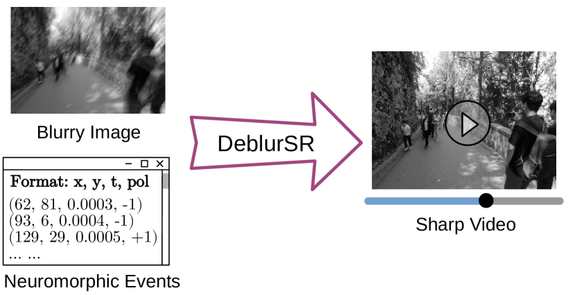
Figure 1: Problem Description. Imagine we are holding a camera while walking on the street. Relative movement between the camera and its surroundings causes motion blur, a visual artifact commonly observed by unprofessional photographers. With the help of neuromorphic events, which are a list of 4D points describing the coordinates, time, and polarity of intensity changes, DeblurSR converts the blurry image we take into a sharp video describing the camera’s motion trajectory during the exposure interval.

One interesting yet under-explored solution is to approximate the sharp output video by per-pixel parametric mappings from time to intensity and use deep learning to regress the parametric coefficients (Song, Huang, and Bajaj 2022). This allows the algorithm to fully exploit the speed of event cameras because the output theoretically has an infinitely high frame rate. However, common parametric kernels such as polynomial and trigonometric functions inherently assume that the underlying intensity signal is smooth and continuous. In reality, a sharp video contains numerous visual features that strongly contrast the background. The movement of a white object before a black background leads to instantaneous intensity flips between the two most extreme pixel values. It creates discontinuities in the intensity signal, which polynomials and trigonometric functions cannot represent. As the only existing work that uses per-pixel parametric mappings to represent videos with arbitrarily high frame rates, E-CIR (Song, Huang, and Bajaj 2022) relies on a refinement module independent of the continuous parameterization to compensate for its limited representation capacity, resulting in a monolithic inefficient two-stage pipeline.

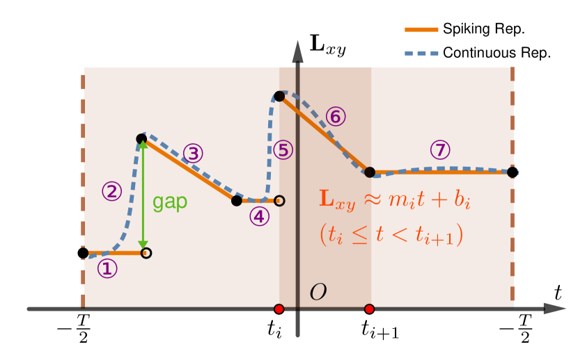
Figure 2: The Spiking Representation. Let $\mathbf{L}_{xy}(t)$ be the intensity of pixel $(x,y)$ at time $t$. $\mathbf{L}_{xy}(t)$ is approximated by a piece-wise linear function, analogous to the membrane potential of the neuron on the retina dedicated to pixel $(x,y)$. ① ④ ⑦: The membrane potential does not change when the neuron is at rest. The pixel’s intensity stays constant in the absence of motion. ② ⑤: Spikes occur at segment endpoints. The gap resembles the strength of the spike, which captures edge features caused by instantaneous changes. ③ ⑥: The slope simulates the rate of membrane potential leakage in a biological neuron after its excitement, enabling the spiking representation to model gradual intensity changes. While the spiking representation (orange) captures signal discontinuities, the continuous parameterization (blue) does not.

As shown in Figure 2, we use a novel Spiking Representation (SR) to approximate the per-pixel mappings from time to intensity. Imagine there is a dedicated visual receptor neuron for each pixel on the human retina. We model the light intensity of each pixel as the membrane potential of the corresponding receptor neuron, defined as the voltage difference between the interior and the exterior of the neuron cell. The spiking representation exploits a piece-wise linear function similar to the one developed by neuroscientists in the 1900s under the name of the Leaky-Integrate-and-Fire model (Lapicque 1907). Each linear segment’s slope characterizes the gradual intensity change rate over time. The gaps at segment endpoints represent abrupt intensity changes caused by the edge movements. The spiking parameters, including the slope and intercept of each line segment and the segment endpoints, are predicted by a deep neural network. We further integrate the per-pixel piece-wise linear parameterization with spatial convolutional kernels, encouraging information to propagate among neighboring pixels. We refer to the proposed intensity modeling as the spiking representation because it mimics the spiking mechanism in biological neurons.

We conduct extensive experimental analysis on the REDS dataset (Nah et al. 2019) with synthetic events and the HQF dataset (Stoffregen et al. 2020) with real events. DeblurSR improves state-of-the-art reconstruction quality by 12.3% on REDS and 22.2% on HQF, while requiring a shorter training time and fewer computing resources. Through ablation studies, we demonstrate the strengths of three optional components, including the automatic keypoint selection module, the integral normalization constant, and the kernel-based spatial modeling. Finally, we show how DeblurSR naturally extends to video super resolution, improving the state-of-the-art method by 7.8%.

In summary, we make the following contributions:

• We propose a novel Spiking Representation (SR) to parameterize sharp videos. We discuss the similarity between the spikes and the biological neural mechanism. We explain how the gaps in the spiking representation can be used to capture sharp edges.

• We train a deep network that regresses the spiking parameters from a blurry image and its associated events during the exposure interval. We show how to use the predicted parameters to render sharp videos.

• In addition to motion deblurring, we extend the spiking representation to support video super resolution.

2 Related Work

2.1 Event Cameras and Spiking Neural Networks

Event cameras (Lichtsteiner, Posch, and Delbruck 2008; Mahowald 1992) react to intensity changes and produce a stream of events. Each event is represented as a 4-tuple $(x,y,t,p)$, including the pixel coordinates, the timestamp, and the binary polarity of the intensity change. Modern event cameras are able to detect up to one million events per second, allowing them to capture extremely fast motion details. However, events are noisy and unable to account for the exact magnitudes of the intensity changes, leading to challenges in algorithm design. A thorough introduction to the technical properties of event cameras is beyond the scope of this paper. We refer interested readers to Gallego et al. (2020) for a comprehensive survey.

Spiking Neural Networks (SNNs) (Maass 1997) are popular tools to build an event-based vision system because both event cameras and SNNs simulate how biological neurons behave. Different mathematical models are constructed to explain the spiking mechanism (Lapicque 1907; Dutta et al. 2017; Hodgkin and Huxley 1952; Izhikevich 2003; Borisyuk and Borisyuk 1997). Our work is particularly inspired by the Leaky-Integrate-and-Fire (LIF) model (Lapicque 1907), where each neuron has a membrane potential whose value decays linearly with time in the logarithmic space and plunges abruptly whenever there is a spike. While prior works in event vision exploit SNNs as a black-box inference network (O’Connor et al. 2013; Diehl et al. 2015; Esser et al. 2016; Rueckauer et al. 2017; Zhang et al. 2021b; Zhu et al. 2022; Zhang et al. 2022; Lee, Kosta, and Roy 2022), we extend the LIF model to directly model intensity changes in a video under the spiking representation. For readers familiar with SNNs, the most significant difference between SNNs and DeblurSR is that SNNs implicitly store the membrane potential and explicitly output the spikes, whereas DeblurSR explicitly models the membrane potential of visual receptor neurons and implicitly represents the spikes through parameterized coefficients.

2.2 Motion Deblurring

Motion deblurring algorithms turn a blurry image into a sharp video, allowing humans and downstream vision applications to understand movements during the image formation process. Motion deblurring is an ill-posed problem because the blurry image alone fails to capture critical motion parameters such as the moving direction and speed (Jin, Meishvili, and Favaro 2018; Purohit, Shah, and Rajagopalan 2019). In Figure 1, it is impossible to tell whether the photographer is moving forward into the woods or backward out of the screen from the blurry image itself. Thanks to the fast data rate of event cameras, several prior works utilize event streams to supplement the blurry input image to address the motion ambiguity (Pan et al. 2019, 2020; Jiang et al. 2020; Lin et al. 2020; Wang et al. 2020; Shang et al. 2021; Zhang et al. 2021a; Han et al. 2021; Xu et al. 2021; Tulyakov et al. 2021; Paikin et al. 2021; Tulyakov et al. 2022; Zhang and Yu 2022; Song, Huang, and Bajaj 2022; Sun et al. 2022; Kim et al. 2021; Wang et al. 2019) in not only image-to-video deblurring but also image-to-image deblurring and frame interpolation. Closely related to our design, E-CIR (Song, Huang, and Bajaj 2022) represents pixel intensities in the output video as polynomial functions characterized by the temporal derivatives as selected event timestamps. This paper argues that the continuous nature of the polynomial representation limits the ability of E-CIR to generate sharp videos. On the other hand, the proposed spiking representation resembles the same biological principle that is followed by event cameras determining how neurons communicate with each other in living organisms, allowing DeblurSR to represent sharp discontinuous edges and enjoy strong interpretability.

3 Method

3.1 Event Camera Principles

On a pixel grid with resolution $h\times w$, let $\mathbf{L}_{xy}(t)$ be the intensity of pixel $(x,y)$ at time $t$. In the natural logarithmic space, consider the amount of intensity change from the previous timestamp $t^{\prime}$ to the current timestamp $t$:

$$\Delta ln[\mathbf{L}_{xy}(t)]=ln[\mathbf{L}_{xy}(t)]-ln[\mathbf{L}_{xy}(t^{\prime})]$$ (1)

At time $t$, an event, $(x,y,t,p)$, indicates that for pixel $(x,y)$, the instantaneous intensity change exceeds the event generation threshold:

$$\Delta ln[\mathbf{L}_{xy}(t)]\geq c^{+} \text{, if }p=1$$

$$\Delta ln[\mathbf{L}_{xy}(t)]\leq c^{-} \text{, if }p=-1$$ (2)

where $p=\pm 1$ is the polarity of the event; $c^{+}$ and $c^{-}$ are event generation thresholds corresponding to positive events (intensity increments) and negative events (intensity decrements), respectively.

Modern event cameras simultaneously capture a stream of high-speed events and another stream of low-speed conventional frames. Let $\mathbf{B}$ be the $h\times w$ conventional frame captured during an exposure interval $[-\frac{T}{2},\frac{T}{2}]$ with length $T$. Mathematically, the conventional frame is the temporal average of the true physical intensities:

$$\mathbf{B}_{xy}=\frac{1}{T}\int_{-\frac{T}{2}}^{\frac{T}{2}}\mathbf{L}_{xy}(t)dt$$ (3)

During the exposure interval, relative motion between the camera and environment leads to undesirable blurriness in the conventional frame capture $\mathbf{B}$, which is a visual artifact commonly observed by unprofessional photographers.

3.2 Problem Description

As illustrated by Figure 1, the input to the event-based motion deblurring problem includes a blurry image $\mathbf{B}=\{\mathbf{B}_{xy}\}$ and all the events $\mathbf{E}=\{(x,y,t,p)|-\frac{T}{2}\leq t\leq\frac{T}{2}\}$ occurred during the exposure interval. The output of the problem is a sharp video with a temporal range of $[-\frac{T}{2},\frac{T}{2}]$.

3.3 Prediction Algorithm

The Spiking Representation. For each pixel $(x,y)$, we propose to approximate its latent intensity $\mathbf{L}_{xy}(t)$ as a parametric mapping from the temporal space $[-\frac{T}{2},\frac{T}{2}]$ to the normalized intensity space $[0,1]$. This contrasts with the conventional video representation, where $\mathbf{L}_{xy}(t)$ is characterized by discrete samples uniformly distributed across the exposure interval, and enjoys the advantage of having an infinitely high frame rate. Given a blurry image and its associated events, our algorithm learns to predict the coefficients of latent intensity parametric mappings for all the pixels. As shown in Figure 2, the proposed spiking representation uses disconnected line segments to approximate the per-pixel intensity mappings. Within each segment, the coefficients include the slope and the intercept.

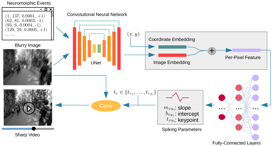
Figure 3: The Overall Pipeline. Given a blurry image and its associated events in the exposure interval, we apply a Convolutional Neural Network (CNN) to extract an image embedding with the same spatial resolution as the input. For each pixel $(x,y)$, we fuse the image embedding with the coordinate embedding using the addition operation. A group of fully-connected layers take the resulting per-pixel feature vector as input and regress the spiking parameters for each pixel as output. At time $t_{r}$, we assemble a spatially varying kernel from the predicted spiking parameters. The convolution of this kernel with the input blurry image gives the output sharp frame at time $t_{r}$. By changing the timestamps, the spiking representation allows DeblurSR to render a sharp video with an arbitrarily high frame rate.

Automatic Keypoint Selection Scheme. As illustrated in Figure 2, a piecewise linear function with $n$ pieces has $n+1$ endpoints. In this paper, we use the term keypoints to refer to the timestamps of these endpoints when the spikes happen. For each pixel $(x,y)$, the sharp intensity $\mathbf{L}_{xy}(t)$ is parameterized by $n$ slopes, $n$ intercepts, and $n+1$ keypoints:

$$\mathbf{L}_{xy}(t)\approx\begin{cases}m_{{xy}_{1}}t+b_{{xy}_{1}}&t_{{xy}_{1}}\leq t<t_{{xy}_{2}}\\ m_{{xy}_{2}}t+b_{{xy}_{2}}&t_{{xy}_{2}}\leq t<t_{{xy}_{3}}\\ \dots\\ m_{{xy}_{n}}t+b_{{xy}_{n}}&t_{{xy}_{n}}\leq t\leq t_{{xy}_{n+1}}\\ \end{cases}$$ (4)

Semantically, a keypoint represents a critical moment when the pixel’s intensity changes significantly, which has a natural correlation to the event generation model described in Equation (2). However, the raw event data is highly irregular. During the exposure interval, different pixels have vastly different numbers of events, presenting a substantial challenge for efficient computation in parallel. Events are also known to be noisy (Pan et al. 2019; Wang et al. 2020; Zhang and Yu 2022). It is, therefore, inappropriate to directly extract the raw event timestamps as keypoints. To effectively exploit the correlation between events and keypoints while allowing efficient parallel computation, we propose the automatic keypoint selection module that is robust against noise. Given the blurry image and its associated events, we employ a neural network to predict a set of $n$ segment widths for each pixel: $\{w_{{xy}_{1}},w_{{xy}_{2}},\dots,w_{{xy}_{n}}\}$. Through activation functions, we normalize the sum of these widths to the exposure length, $T$. The keypoints are $t_{{xy}_{1}}=-\frac{T}{2}$ and:

$$t_{{xy}_{i}}=t_{{xy}_{i-1}}+w_{{xy}_{i-1}}\quad i=2,3,\dots,n+1$$ (5)

An alternative to the automatic keypoint selection scheme is to use a heuristic-based algorithm to choose the keypoints from all event timestamps. This approach is similar to how E-CIR decides the Lagrange bases for the polynomial functions.

Integral Normalization Constant. The basic version of the spiking representation discussed above may not satisfy the physical model in Equation (3) if the coefficients are predicted by a neural network. To fully utilize the information in the blurry input image, we amend the spiking representation in Equation (4) with a normalization constant $c_{xy}$:

$$\mathbf{L}_{xy}(t)\approx c_{xy}+\begin{cases}m_{{xy}_{1}}t+b_{{xy}_{1}}&t_{{xy}_{1}}\leq t<t_{{xy}_{2}}\\ m_{{xy}_{2}}t+b_{{xy}_{2}}&t_{{xy}_{2}}\leq t<t_{{xy}_{3}}\\ \dots\\ m_{{xy}_{n}}t+b_{{xy}_{n}}&t_{{xy}_{n}}\leq t\leq t_{{xy}_{n+1}}\\ \end{cases}$$ (6)

where, given $m_{{xy}_{i}}$’s, $b_{{xy}_{i}}$’s, and $\mathbf{B}_{xy}$, the value of $c_{xy}$ can be solved analytically from Equation (3) by calculating the indefinite integral of Equation (6):

$$c_{xy}= -\mathbf{B}_{xy}+\frac{1}{2T}\sum_{i=1}^{n}m_{{xy}_{i}}(t_{{xy}_{i+1}}^{2}-t_{{xy}_{i}}^{2})+$$ (7)

$$\frac{1}{T}\sum_{i=1}^{n}b_{i}(t_{{xy}_{i+1}}-t_{{xy}_{i}})$$ (8)

Kernel-Based Spatial Modeling. The sharpness of edges largely determines the quality of motion deblurring. While the above discussion addresses temporal intensity changes, it fails to incorporate spatial brightness variations, which is also key to edge sharpness. To address this issue, we predict $k^{2}$ different sets of spiking parameters for each pixel and use them to assemble a $k\times k$ convolutional kernel $\mathbf{K}_{xy}(t)$. After the spiking representation is further enhanced with spatial kernels, the sharp intensity is given as:

$$\mathbf{L}_{xy}(t)\approx c_{xy}+\mathbf{K}_{xy}(t)\circledast\mathcal{N}(\mathbf{B}_{xy})$$ (9)

where $\circledast$ stands for the inner product operator between two flattened vectors, and $\mathcal{N}(\mathbf{B}_{xy})$ is a $k\times k$ neighborhood for pixel $(x,y)$ in the input blurry image. We refer interested readers to our open-source GitHub repository for implementation details.

Prediction Pipeline. We present the overall motion deblurring pipeline in Figure 3. We first voxelize the irregular event input into an $m\times h\times w$ histogram tensor (Zhu et al. 2019), where $m$ is the number of histogram bins. We then concatenate this histogram tensor with the blurry image, creating an input tensor whose dimensions are $(m+1)\times h\times w$. A UNet (Ronneberger, Fischer, and Brox 2015)-based convolutional neural network takes this concatenated tensor as input and extracts a $d\times h\times w$ dimensional image embedding. Next, we utilize a linear layer to predict another $d$-dimensional coordinate embedding from the 2D coordinates of each pixel. We fuse the pixel-wise image and coordinate embeddings by the addition operation and employ fully-connected layers to regress the spiking parameters, including $k^{2}$ slopes, $k^{2}$ intercepts, and $n$ widths between $n+1$ keypoints for each pixel, where $k$ is the spatial kernel size. The fully connected layers have a total output size of $2k^{2}+n$ Finally, to render a sharp video with $N$ frames, we assemble the spatial kernels at rendering timestamps $\{t_{r_{1}},\dots,t_{r_{N}}\}$ and convolve the kernels with the blurry image. The entire pipeline is trained end-to-end using the L1 loss on reconstructed sharp frames.

Extension to Super Resolution. Thanks to coordinate embedding, DeblurSR can predict the spiking parameters for pixels with non-integer coordinates in between two regular pixels. During testing, the coordinates take non-integer values such as $(1.5,7)$, representing the midpoint of two regular pixels. This allows natural support to video super resolution. Formally, given a blurry image and events defined on an $h\times w$ grid, the super-resolution problem aims at reconstructing a sharp video with a higher resolution $h^{\prime}\times w^{\prime}$. In Section 4.4, we show that DeblurSR achieves state-of-the-art super-resolution performance even without any high-resolution training supervision.

4 Evaluation

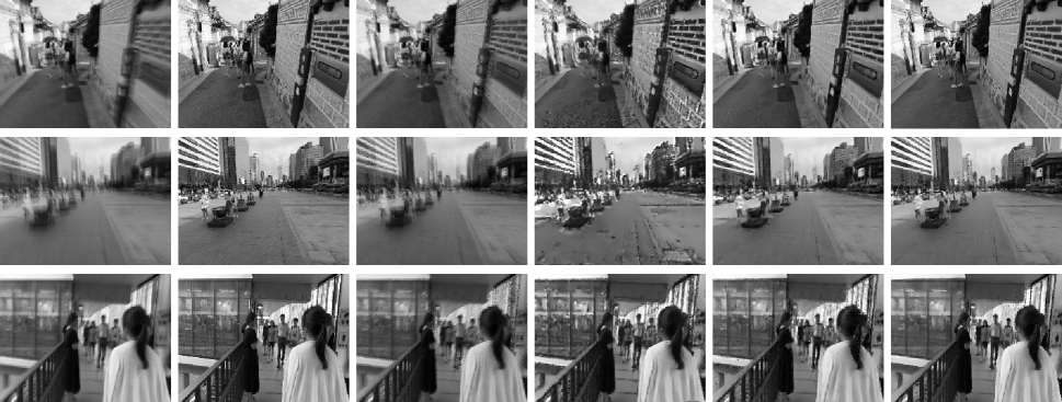
Input

Ground Truth

EDI

eSL-Net

E-CIR

Ours

Figure 4: Visualizations on REDS. Video results are available on our GitHub page with higher illustration quality.

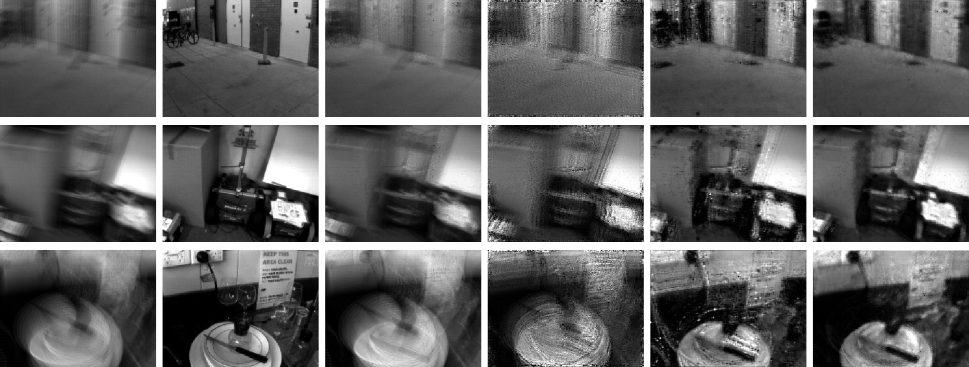
Input

Ground Truth

EDI

eSL-Net

E-CIR

Ours

Figure 5: Visualizations on HQF. Video results are available on our GitHub page with higher illustration quality.

Methods	Performance on REDS			Performance on HQF
	MSE $\downarrow$	PSNR $\uparrow$	SSIM $\uparrow$	MSE $\downarrow$	PSNR $\uparrow$	SSIM $\uparrow$
EDI	0.182	21.663	0.664	0.336	17.822	0.515
eSL-Net	0.203	20.640	0.601	0.452	14.938	0.282
E-CIR	0.114	25.531	0.819	0.207	21.713	0.609
Ours	0.100 $\pm$ 0.001	26.725 $\pm$ 0.001	0.859 $\pm$ 0.001	0.161 $\pm$ 0.001	23.910 $\pm$ 0.008	0.693 $\pm$ 0.001

Table 1: On both the REDS and the HQF datasets, DeblurSR outperforms baseline approaches that represent videos by frames and polynomials in terms of the quantitative motion deblurring quality.

	Modules			MSE $\downarrow$
	AK	IN	KS	REDS	HQF
1	✗	✗	✗	0.107 $\pm$ 0.001	0.236 $\pm$ 0.002
2	✓	✗	✗	0.103 $\pm$ 0.001	0.229 $\pm$ 0.001
3	✓	✓	✗	0.102 $\pm$ 0.001	0.163 $\pm$ 0.001
4	✓	✓	✓	0.100 $\pm$ 0.001	0.161 $\pm$ 0.001

Table 2: We use ablation studies to demonstrate the strengths of the automatic keypoint selection scheme (AK), the integral normalization constant (IN), as well as kernel-based spatial modeling (KS).

4.1 Experimental Setup

We conduct experimental evaluations on two benchmark datasets. The REalistic and Dynamic Scenes (REDS) (Nah et al. 2019) dataset is a popular dataset used to evaluate deblurring approaches. The original REDS dataset contains sharp videos with various real-world contents released under the CC BY 4.0 license. Following Song et al. (2022), we use the ESIM simulator (Rebecq, Gehrig, and Scaramuzza 2018) to synthesize events and blurry images. We then employ the official training and validation splits to train and test our model, respectively. Notably, this dataset is also referred to as the GroPro dataset by some authors (Wang et al. 2020), although a much smaller dataset popular in image-to-image deblurring approaches happens to share the same name (Nah, Kim, and Lee 2017).

The High Quality Frames (HQF) (Stoffregen et al. 2020) dataset is another benchmark recently developed to evaluate event-based vision algorithms. The dataset is available for public download, but the licensing details are unclear. The HQF dataset contains both sharp videos and the associated event captures. We apply temporal averaging to generate blurry images from the sharp video. Following Zhang et al. (2022), we use five clips for testing and nine clips for training.

We compare DeblurSR to all the event-based image-to-video motion deblurring approaches with a complete (data preparation, training, and testing) open-source implementation known to us at the time of paper writing. We additionally evaluate eSL-Net (Wang et al. 2020) by creating customized training scripts for the incomplete code released on GitHub.

4.2 Training Details

We implement DeblurSR under PyTorch (Paszke et al. 2019) and utilize ADAM (Kingma and Ba 2014) to train the network for 50 epochs. We set the initial learning rate to 0.0001 and reduce the learning rate by half after 20 and 40 epochs, respectively. The number of line segments in the spiking representation is $n=10$. The dimension of spatial kernels is $k=3$. The number of histogram bins is $m=26$. The size of image and coordinate embeddings is $d=256$. More details of our experiments are available in the open-source GitHub repository.

4.3 Motion Deblurring

Baseline Comparison. Table 1 presents the quantitative evaluation on the REDS and HQF datasets. We use three image quality metrics to compare DeblurSR with different baseline approaches: the Mean Squared Error (MSE), the Peak Signal-to-Noise Ratio (PSNR), and the Structural Similarity Index Measure (SSIM).

Our method demonstrates an impressive ability in motion deblurring. Specifically, on the REDS dataset, DeblurSR improves the current best-performing method by 12.3% in MSE, 4.7% in PSNR, and 4.9% in SSIM. On HQF, DeblurSR outperforms the state-of-the-art approach by 22.2% in MSE, 10.1% in PSNR, and 14.0% in SSIM.

Qualitatively, as shown in Figure 4 and Figure 5, DeblurSR generates smooth and sharp frames. In particular, we point out that our results are sharper than the EDI reconstruction, which assumes all events correspond to the same amount of intensity change. Meanwhile, our reconstructed frames are significantly less noisy than the eSL-Net reconstruction, which overly emphasizes texture details. Compared with E-CIR, DeblurSR offers more realistic details around the thin edges. The difference between E-CIR and DeblurSR is sometimes subtle and hard to notice from static images.

Efficiency. The proposed DeblurSR is computationally efficient. On REDS, it takes 100 hours to train E-CIR for 50 epochs using three Tesla V100 GPUs. By contrast, DeblurSR only requires 72 hours and two of the same GPUs under the identical training setting, representing a 28.0% reduction in training time and a 33.3% reduction in resource demand. The efficiency comes from the simplicity of our spiking representation in contrast with the high-order polynomial parameterization in E-CIR, which allows faster operations like computing the derivative and integral.

Ablation Study. Table 2 summarizes the quality of motion deblurring using different variants of the model. The comparison between the first and second rows shows that the proposed automatic keypoint selection module improves the heuristic-based keypoint selection algorithm in E-CIR by 3.7% on REDS and 3.0% on HQF. This result demonstrates the advantage of learning the critical timestamps from a large amount of training data.

From the second row to the third row, the integral normalization constant improves the deblurring quality by 1.0% and 29.0% on REDS and HQF, respectively. The improvement suggests that the physical model discussed in Equation (3) is an effective regularization for the neuromorphic spiking parameters. Noticeably, the improvement on HQF is a lot more significant than REDS. While REDS is a large synthetic dataset with 240 training clips, HQF is a small real benchmark with only 9 training clips. Empirically, we observe that the normalization constant is particularly beneficial when data is limited and the event noise is real and complex.

Finally, the last two rows in Table 2 examine the effectiveness of the spatial convolutional kernel modeling. The spatial kernel leads to 2.0% and 0.6% MSE improvement on REDS and HQF, respectively. Importantly, the kernel-based spatial modeling demonstrates that the spiking representation can also be used as an operator on the input and support complex structures. A promising future direction is to stack layers of such operators and construct a network.

4.4 Super Resolution

Methods	MSE $\downarrow$	PSNR $\uparrow$	SSIM $\uparrow$
EDI (+bicubic)	0.196	20.789	0.550
eSL-Net	0.228	19.507	0.483
E-CIR (+bicubic)	0.142	23.530	0.622
Ours (LR supervision)	0.140	23.642	0.634
Ours (HR supervision)	0.131	24.272	0.664

Table 3: We extend DeblurSR to super-resolution and evaluate the performance on the REDS dataset.

As illustrated in Figure 3, DeblurSR naturally supports super resolution because the pixel coordinates $(x,y)$ can take non-integer values such as $(1.5,7)$, representing the midpoint of two regular pixels. This section compares DeblurSR with three different baseline approaches on the REDS dataset. We provide the blurry image and the events in low resolution ($180\times 240$) and evaluate the results in high resolution ($720\times 960$). Among the three baseline approaches, we note that only eSL-Net uses ground-truth high-resolution frames in the training objective. Neither EDI nor E-CIR provides intrinsic support to super-resolution. We obtain high-resolution outputs from EDI and E-CIR through bicubic interpolation. From Table 3, we observe that DeblurSR achieves state-of-the-art performance with and without high-resolution supervision. In the absence of high-resolution supervision, DeblurSR improves E-CIR by 1.4% in MSE. With high-resolution supervision, the relative improvement becomes 7.8%. Figure 6 further confirms our advantage through qualitative visualizations.

5 Conclusion

In this paper, we introduce DeblurSR, a novel event-based motion deblurring approach based on the spiking representation. DeblurSR builds upon the same biological principles followed by the event camera design. Experiments show that DeblurSR outperforms state-of-the-art approaches in deblurring quality and can be easily extended to video super resolution. In the future, we plan to modify DeblurSR and allow different pixels to have a different number of parametric segments. This requires a non-trivial redesign of the prediction network to handle the heterogeneity. Another possible direction is to construct a general-purpose deep network with layers of spiking neurons.

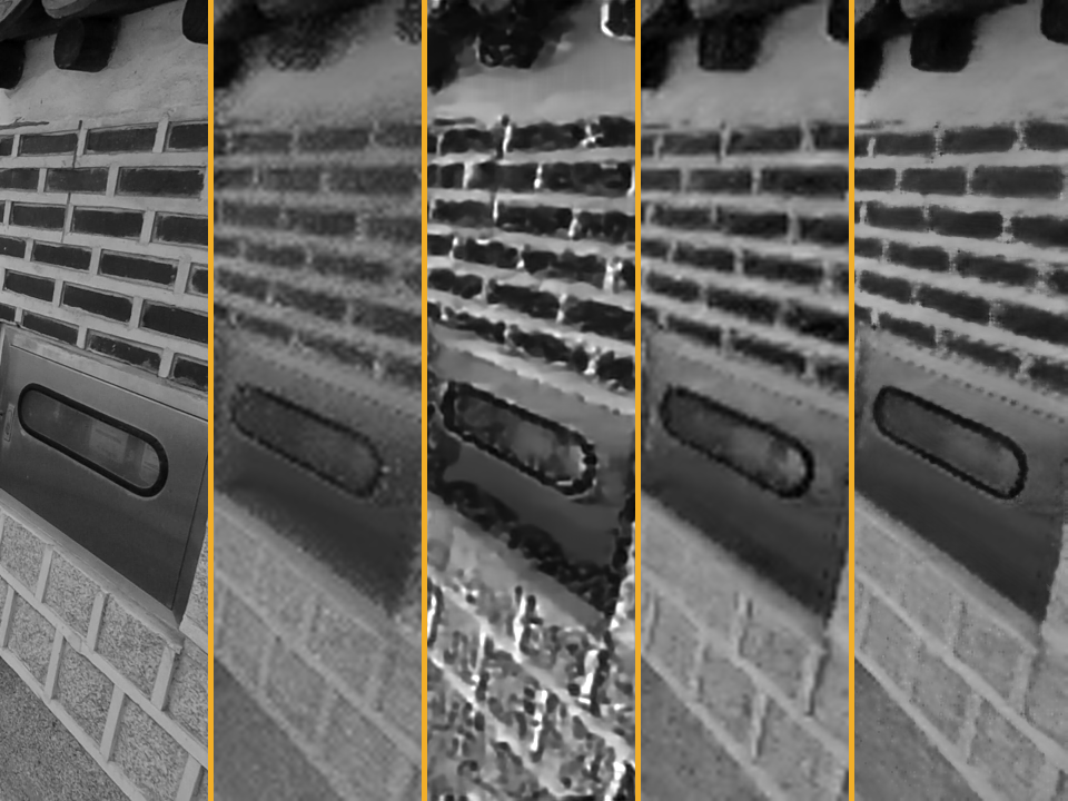
(a)

(b)

(c)

(d)

(e)

Figure 6: Visual Comparison Between Different Super-Resolution Methods. (a) Ground Truth; (b) EDI; (c) eSL-Net; (d) E-CIR; (e) Ours.

References

- Borisyuk and Borisyuk (1997) Borisyuk, R. M.; and Borisyuk, G. N. 1997. Information coding on the basis of synchronization of neuronal activity. BioSystems, 40(1-2): 3–10.
- Diehl et al. (2015) Diehl, P. U.; Neil, D.; Binas, J.; Cook, M.; Liu, S.; and Pfeiffer, M. 2015. Fast-classifying, high-accuracy spiking deep networks through weight and threshold balancing. In 2015 International Joint Conference on Neural Networks (IJCNN), 1–8.
- Dutta et al. (2017) Dutta, S.; Kumar, V.; Shukla, A.; Mohapatra, N. R.; and Ganguly, U. 2017. Leaky integrate and fire neuron by charge-discharge dynamics in floating-body MOSFET. Scientific reports, 7(1): 1–7.
- Esser et al. (2016) Esser, S. K.; Merolla, P. A.; Arthur, J. V.; Cassidy, A. S.; Appuswamy, R.; Andreopoulos, A.; Berg, D. J.; McKinstry, J. L.; Melano, T.; Barch, D. R.; et al. 2016. Convolutional networks for fast, energy-efficient neuromorphic computing. Proceedings of the national academy of sciences, 113(41): 11441–11446.
- Gallego et al. (2020) Gallego, G.; Delbruck, T.; Orchard, G. M.; Bartolozzi, C.; Taba, B.; Censi, A.; Leutenegger, S.; Davison, A.; Conradt, J.; Daniilidis, K.; and Scaramuzza, D. 2020. Event-based Vision: A Survey. IEEE Transactions on Pattern Analysis and Machine Intelligence, 1–1.
- Han et al. (2021) Han, J.; Yang, Y.; Zhou, C.; Xu, C.; and Shi, B. 2021. EvIntSR-Net: Event Guided Multiple Latent Frames Reconstruction and Super-Resolution. In Proceedings of the IEEE/CVF International Conference on Computer Vision, 4882–4891.
- Hodgkin and Huxley (1952) Hodgkin, A. L.; and Huxley, A. F. 1952. A quantitative description of membrane current and its application to conduction and excitation in nerve. The Journal of physiology, 117(4): 500.
- Izhikevich (2003) Izhikevich, E. M. 2003. Simple model of spiking neurons. IEEE Transactions on neural networks, 14(6): 1569–1572.
- Jiang et al. (2020) Jiang, Z.; Zhang, Y.; Zou, D.; Ren, J.; Lv, J.; and Liu, Y. 2020. Learning event-based motion deblurring. In Proceedings of the IEEE/CVF Conference on Computer Vision and Pattern Recognition, 3320–3329.
- Jin, Meishvili, and Favaro (2018) Jin, M.; Meishvili, G.; and Favaro, P. 2018. Learning to extract a video sequence from a single motion-blurred image. In Proceedings of the IEEE Conference on Computer Vision and Pattern Recognition, 6334–6342.
- Kim et al. (2021) Kim, T.; Lee, J.; Wang, L.; and Yoon, K.-J. 2021. Event-guided Deblurring of Unknown Exposure Time Videos. arXiv preprint arXiv:2112.06988.
- Kingma and Ba (2014) Kingma, D. P.; and Ba, J. 2014. Adam: A method for stochastic optimization. arXiv preprint arXiv:1412.6980.
- Lapicque (1907) Lapicque, L. 1907. Recherches quantitatives sur l’excitation electrique des nerfs traitee comme une polarization. Journal de physiologie et de pathologie générale, 9: 620–635.
- Lee, Kosta, and Roy (2022) Lee, C.; Kosta, A. K.; and Roy, K. 2022. Fusion-FlowNet: Energy-efficient optical flow estimation using sensor fusion and deep fused spiking-analog network architectures. In 2022 International Conference on Robotics and Automation (ICRA), 6504–6510. IEEE.
- Lichtsteiner, Posch, and Delbruck (2008) Lichtsteiner, P.; Posch, C.; and Delbruck, T. 2008. A 128 128 120 dB 15 s Latency Asynchronous Temporal Contrast Vision Sensor. IEEE Journal of Solid-State Circuits, 43(2): 566–576.
- Lin et al. (2020) Lin, S.; Zhang, J.; Pan, J.; Jiang, Z.; Zou, D.; Wang, Y.; Chen, J.; and Ren, J. 2020. Learning event-driven video deblurring and interpolation. In Computer Vision–ECCV 2020: 16th European Conference, Glasgow, UK, August 23–28, 2020, Proceedings, Part VIII 16, 695–710. Springer.
- Maass (1997) Maass, W. 1997. Networks of spiking neurons: The third generation of neural network models. Neural Networks, 10(9): 1659–1671.
- Mahowald (1992) Mahowald, M. 1992. VLSI analogs of neuronal visual processing: a synthesis of form and function. Ph.D. thesis, California Institute of Technology.
- Nah et al. (2019) Nah, S.; Baik, S.; Hong, S.; Moon, G.; Son, S.; Timofte, R.; and Lee, K. M. 2019. NTIRE 2019 Challenge on Video Deblurring and Super-Resolution: Dataset and Study. In CVPR Workshops.
- Nah, Kim, and Lee (2017) Nah, S.; Kim, T. H.; and Lee, K. M. 2017. Deep Multi-Scale Convolutional Neural Network for Dynamic Scene Deblurring. In CVPR.
- O’Connor et al. (2013) O’Connor, P.; Neil, D.; Liu, S.-C.; Delbruck, T.; and Pfeiffer, M. 2013. Real-time classification and sensor fusion with a spiking deep belief network. Frontiers in neuroscience, 7: 178.
- Paikin et al. (2021) Paikin, G.; Ater, Y.; Shaul, R.; and Soloveichik, E. 2021. EFI-Net: Video Frame Interpolation From Fusion of Events and Frames. In Proceedings of the IEEE/CVF Conference on Computer Vision and Pattern Recognition (CVPR) Workshops, 1291–1301.
- Pan et al. (2020) Pan, L.; Hartley, R.; Scheerlinck, C.; Liu, M.; Yu, X.; and Dai, Y. 2020. High frame rate video reconstruction based on an event camera. IEEE Transactions on Pattern Analysis and Machine Intelligence.
- Pan et al. (2019) Pan, L.; Scheerlinck, C.; Yu, X.; Hartley, R.; Liu, M.; and Dai, Y. 2019. Bringing a blurry frame alive at high frame-rate with an event camera. In Proceedings of the IEEE Conference on Computer Vision and Pattern Recognition, 6820–6829.
- Paszke et al. (2019) Paszke, A.; Gross, S.; Massa, F.; Lerer, A.; Bradbury, J.; Chanan, G.; Killeen, T.; Lin, Z.; Gimelshein, N.; Antiga, L.; Desmaison, A.; Kopf, A.; Yang, E.; DeVito, Z.; Raison, M.; Tejani, A.; Chilamkurthy, S.; Steiner, B.; Fang, L.; Bai, J.; and Chintala, S. 2019. PyTorch: An Imperative Style, High-Performance Deep Learning Library. In Wallach, H.; Larochelle, H.; Beygelzimer, A.; d'Alché-Buc, F.; Fox, E.; and Garnett, R., eds., Advances in Neural Information Processing Systems 32, 8024–8035. Curran Associates, Inc.
- Purohit, Shah, and Rajagopalan (2019) Purohit, K.; Shah, A.; and Rajagopalan, A. 2019. Bringing alive blurred moments. In Proceedings of the IEEE/CVF Conference on Computer Vision and Pattern Recognition, 6830–6839.
- Rebecq, Gehrig, and Scaramuzza (2018) Rebecq, H.; Gehrig, D.; and Scaramuzza, D. 2018. ESIM: an Open Event Camera Simulator. Conf. on Robotics Learning (CoRL).
- Ronneberger, Fischer, and Brox (2015) Ronneberger, O.; Fischer, P.; and Brox, T. 2015. U-net: Convolutional networks for biomedical image segmentation. In International Conference on Medical image computing and computer-assisted intervention, 234–241. Springer.
- Rueckauer et al. (2017) Rueckauer, B.; Lungu, I.-A.; Hu, Y.; Pfeiffer, M.; and Liu, S.-C. 2017. Conversion of continuous-valued deep networks to efficient event-driven networks for image classification. Frontiers in neuroscience, 11: 682.
- Shang et al. (2021) Shang, W.; Ren, D.; Zou, D.; Ren, J. S.; Luo, P.; and Zuo, W. 2021. Bringing Events Into Video Deblurring With Non-Consecutively Blurry Frames. In Proceedings of the IEEE/CVF International Conference on Computer Vision, 4531–4540.
- Song, Huang, and Bajaj (2022) Song, C.; Huang, Q.; and Bajaj, C. 2022. E-CIR: Event-Enhanced Continuous Intensity Recovery. In Proceedings of the IEEE/CVF Conference on Computer Vision and Pattern Recognition, 7803–7812.
- Stoffregen et al. (2020) Stoffregen, T.; Scheerlinck, C.; Scaramuzza, D.; Drummond, T.; Barnes, N.; Kleeman, L.; and Mahony, R. 2020. Reducing the sim-to-real gap for event cameras. In European Conference on Computer Vision, 534–549. Springer.
- Sun et al. (2022) Sun, L.; Sakaridis, C.; Liang, J.; Jiang, Q.; Yang, K.; Sun, P.; Ye, Y.; Wang, K.; and Van Gool, L. 2022. Event-Based Fusion for Motion Deblurring with Cross-modal Attention. In European Conference on Computer Vision (ECCV).
- Tulyakov et al. (2022) Tulyakov, S.; Bochicchio, A.; Gehrig, D.; Georgoulis, S.; Li, Y.; and Scaramuzza, D. 2022. Time Lens++: Event-based Frame Interpolation with Parametric Non-linear Flow and Multi-scale Fusion. In Proceedings of the IEEE/CVF Conference on Computer Vision and Pattern Recognition, 17755–17764.
- Tulyakov et al. (2021) Tulyakov, S.; Gehrig, D.; Georgoulis, S.; Erbach, J.; Gehrig, M.; Li, Y.; and Scaramuzza, D. 2021. Time Lens: Event-Based Video Frame Interpolation. In Proceedings of the IEEE/CVF Conference on Computer Vision and Pattern Recognition, 16155–16164.
- Wang et al. (2020) Wang, B.; He, J.; Yu, L.; Xia, G.-S.; and Yang, W. 2020. Event Enhanced High-Quality Image Recovery. In European Conference on Computer Vision. Springer.
- Wang et al. (2019) Wang, Z. W.; Jiang, W.; He, K.; Shi, B.; Katsaggelos, A.; and Cossairt, O. 2019. Event-driven video frame synthesis. In Proceedings of the IEEE/CVF International Conference on Computer Vision Workshops, 0–0.
- Xu et al. (2021) Xu, F.; Yu, L.; Wang, B.; Yang, W.; Xia, G.-S.; Jia, X.; Qiao, Z.; and Liu, J. 2021. Motion Deblurring with Real Events. In Proceedings of the IEEE/CVF International Conference on Computer Vision, 2583–2592.
- Zhang et al. (2022) Zhang, J.; Dong, B.; Zhang, H.; Ding, J.; Heide, F.; Yin, B.; and Yang, X. 2022. Spiking Transformers for Event-Based Single Object Tracking. In Proceedings of the IEEE/CVF Conference on Computer Vision and Pattern Recognition, 8801–8810.
- Zhang et al. (2021a) Zhang, L.; Zhang, H.; Zhu, C.; Guo, S.; Chen, J.; and Wang, L. 2021a. Fine-Grained Video Deblurring with Event Camera. In International Conference on Multimedia Modeling, 352–364. Springer.
- Zhang et al. (2021b) Zhang, X.; Liao, W.; Yu, L.; Yang, W.; and Xia, G.-S. 2021b. Event-based synthetic aperture imaging with a hybrid network. In Proceedings of the IEEE/CVF Conference on Computer Vision and Pattern Recognition, 14235–14244.
- Zhang and Yu (2022) Zhang, X.; and Yu, L. 2022. Unifying Motion Deblurring and Frame Interpolation with Events. In Proceedings of the IEEE/CVF Conference on Computer Vision and Pattern Recognition, 17765–17774.
- Zhu et al. (2019) Zhu, A. Z.; Yuan, L.; Chaney, K.; and Daniilidis, K. 2019. Unsupervised Event-Based Learning of Optical Flow, Depth, and Egomotion. In Proceedings of the IEEE/CVF Conference on Computer Vision and Pattern Recognition (CVPR).
- Zhu et al. (2022) Zhu, L.; Wang, X.; Chang, Y.; Li, J.; Huang, T.; and Tian, Y. 2022. Event-based Video Reconstruction via Potential-assisted Spiking Neural Network. In Proceedings of the IEEE/CVF Conference on Computer Vision and Pattern Recognition, 3594–3604.