Optimal control of distributed ensembles
with application to Bloch equations^∗

Abstract

Motivated by the problem of designing robust composite pulses for Bloch equations in the presence of natural perturbations, we study an abstract optimal ensemble control problem in a probabilistic setting with a general nonlinear performance criterion. The model under study addresses mean-field dynamics described by a linear continuity equation in the space of probability measures. For the resulting optimization problem, we derive an exact representation of the increment of the cost functional in terms of the flow of the driving vector field. Relying on the exact increment formula, a descent method is designed that is free of any internal line search. The numerical method is applied to solve new control problems for distributed ensembles of Bloch equations.

I MOTIVATION

Consider a population of homotypic individuals labeled by the points $\omega$ of some set $\Omega$. The state of the $\omega$th object at the time moment $t$, $x(t,\omega)\in\mathbb{R}^{n}$, evaluates on a given time interval $I\doteq[0,T]$ under the action of the parameterized vector field $V:\,\mathbb{R}^{n}\times\mathbb{R}^{s}\times U\to\mathbb{R}^{n}$, starting from a given position $x_{0}(\omega)\in\mathbb{R}^{n}$:

$$\left\{\begin{array}[]{l}\partial_{t}x(t,\omega)=V_{u}\left(x(t,\omega),\eta(\omega)\right)\\[5.69046pt] x(0,\omega)=x_{0}(\omega)\end{array}\right|\quad\omega\in\Omega.$$ (1)

The dynamics (1) involves two types of structural “parameters”: the function $\eta:\,\Omega\to\mathbb{R}^{s}$ manifests disturbances or structural variations of the underlying model, while an exogenous signal $u$ with values in a given set $U\subseteq\mathbb{R}^{m}$ models the control action.

In the simplest case, the parameterization space $\Omega$ is just a finite set of indexes, and (1) reduces to a multi-agent system of non-interacting units. In a more general setup, we deal with the continuum of individuals moving in a discoordinated way. Commonly, in such models, $\Omega$ is a simply organized compact subset of $\mathbb{R}^{s}$, and $\eta$ is the identity mapping $\Omega\to\Omega$.

Problems of ensemble control arise when one has to design a control signal in a “broadcast” way, i.e., such that it acts simultaneously on all individual trajectories $x(\cdot,\omega)$, $\omega\in\Omega$, to force them towards a desired behavior; this means that $u$ should be a function $t\mapsto u(t)$ of time variable only (independent of $\omega$).

A canonical example is the problem of designing external excitations of quantum ensembles. Pioneering works in this area were focused on the famous Bloch equation [1, 2], which models the macroscopic evolution of bulk magnetization in a population of non-interacting nuclear spins immersed in an intense static magnetic field, which is modulated by the radio frequency (rf-) field. In nuclear magnetic resonance (NMR) experiments, the strength of the applied magnetic field is subject to unavoidable perturbations (static- and/or rf-field inhomogeneity), while the spin ensembles demonstrate perceptible variations in their dissipation rates and/or natural frequencies (Larmor dispersion). The related problem of control engineering is to design robust signals (so-called composite pulses) compensating for the mentioned disturbances; mathematically, this task can be formalized as a problem of optimal ensemble control, see, e.g. [3]. In NMR spectroscopy, the designed pulse sequences are typically desired to be selective, i.e., some sub-populations (with prescribed Larmor frequencies) have to be excited, while the other ones should remain intact or saturated [4]; such are, e.g., contrast problems in NMR imaging [5, 6]. In the language of ensemble control, this means to drive several uncoupled populations of spins by a common magnetic field.

I-A Probabilistic Setup. Distributed Ensembles

In contrast to [7, 6, 5], our approach stems from the probabilistic interpretation of the ensemble dynamics, assuming that $\Omega$ is endowed with the structure of probability space $(\Omega,\mathcal{A},\mathbb{P})$ with a specified $\sigma$-algebra $\mathcal{A}\subset 2^{\Omega}$ and a canonical probability measure $\mathbb{P}$ on $(\Omega,\mathcal{F})$ (we shall write $\mathbb{P}\in\mathcal{P}(\Omega)$).

This interpretation is motivated by practical applications, in which the individual states $x(\cdot,\omega)$ can not be measured directly, and all the available information is based on some “observables” – measurement outputs accompanying the dynamics (1) and involving certain statistical characteristics, see, e.g., [8].

In the probabilistic setup, the map $(t,\omega)\mapsto(x(t,\omega),\eta(\omega))$ is naturally viewed as a deterministic random process, and the behavior of the random variable $\omega\mapsto(x(t,\omega),\eta(\omega))$ can be analyzed by investigating the time-evolution of its law

$$\varrho_{t}=\left(x(t,\cdot),\eta(\cdot)\right)_{\sharp}\mathbb{P}\in\mathcal{P}(\mathbb{R}^{n+s}).$$ (2)

Hereinafter, the operator $F_{\sharp}:\,\mathcal{P}(\mathcal{X})\to\mathcal{P}(\mathcal{Y})$ denotes the pushforward of a measure $\mu\in\mathcal{P}(\mathcal{X})$ through a (Borel) map $F:\,\mathcal{X}\to\mathcal{Y}$ between two measurable spaces that acts on functions $\varphi:\,\mathcal{Y}\to\mathbb{R}$ with the property $\varphi\circ F\in L_{1}(\mathcal{X};\mu)$ by the rule

$$\int_{\mathcal{Y}}\!\!\varphi\,d(F_{\sharp}\mu)=\int_{\mathcal{X}}\!\!\varphi\circ F\,d\mu.$$ (3)

Under the standard regularity of the map $(x,\eta)\mapsto V_{\upsilon}(x,\eta)$, the measure-valued curve $t\mapsto\varrho_{t}$ is a unique distributional solution of the continuity equation [9]

$$\partial_{t}\varrho_{t}+\nabla_{x}\cdot\left(V_{u(t)}\,\varrho_{t}\right)=0,\quad\varrho_{0}=(x_{0}(\cdot),\eta(\cdot))_{\sharp}\mathbb{P};$$ (4)

$\nabla_{x}$ denotes the gradient w.r.t. $x\in\mathbb{R}^{n}$, and “$\cdot$” means the scalar product.

The discussed interpretation of (1) postulates a passage from the multi-particle, microscopic model represented by many copies of an ODE to a distributed, macroscopic representation described by a PDE and called the mean field; systems (1) and (4) are the so-called Lagrangian and Eulerian forms of the mean-field dynamics, respectively [10].

Remark that, as a result of this passage, a nonlinear finite-dimensional object is replaced by an infinite-dimensional but state-linear ($\varrho$-linear) one. The linearity of the reduced model plays a vital role in our study as it gives rise to an exact representation of the increment ($\infty$-order variation) of the cost functional in the corresponding optimal control problem to be presented in § IV.

Finally, observe that PDE (4) can be viewed as a family $\eta\mapsto\mu^{\eta}_{t}$ of $\mathcal{P}(\mathbb{R}^{n})$-valued curves solving, $\Xi$-a.e., the “sliced” continuity equation of the same structure with the vector field $V^{\eta}\doteq V(\cdot,\eta)$ and initial condition $\mu^{\eta}_{0}=\vartheta^{\eta}\in\mathcal{P}(\mathbb{R}^{n})$, where the map $\eta\mapsto\vartheta^{\eta}$ is obtained by disintegrating the distribution $\varrho_{0}$ w.r.t. the projection $\Xi\doteq((x,\eta)\mapsto\eta)_{\sharp}\varrho_{0}$. We call such a family the distributed ensemble; this concept separates two types of uncertainty: dispersion in the initial data $\omega\mapsto x_{0}(\omega)$ is converted to the mean field, while fluctuations of the dynamics, $\eta\mapsto V^{\eta}$, are treated independently.

I-B Contribution and Novelty

This work contributes to the line of research [7, 5, 6, 3] devoted to optimal control of quantum ensembles. We elaborate on a general approach that captures the natural probabilistic flavor of ensemble control problems. From practical viewpoints, it enables us to improve the quality of designed control signals since it takes into account the available statistical information, and in this way allows us to concentrate the “resource” of feasible control options around relevant values of $\omega$. A key result is the development of a descent algorithm for optimal ensemble control originating from an exact increment formula for the nonlinear cost functional. In contrast to familiar indirect methods [11] based on the 1st variation (i.e. on Pontryagin’s maximum principle, PMP), our approach is free of any hidden parameters and does not involve any internal line search. This essentially improves the computational performance, where the algorithm is proved to converge towards a PMP extremal, but the convergence is, typically, faster than as for the conventional gradient descent. Furthermore – due to the nonlocal nature of the underlying increment formula – our algorithm can step over local solutions, and therefore, has the potential of global search.

This paper generalizes our recent works [12, 13], where the exact increment formula and a nonlocal algorithm were derived for models of linear and linear-quadratic structure. Now, we consider an arbitrary nonlinear cost functional on the space of probability measures, which has the so-called intrinsic derivative (see [14] and the discussion in sec. III-C).

II OPTIMAL CONTROL PROBLEM

First, we introduce some necessary notations: Let $\mathcal{X}$ be a metric space, and $I\doteq[0,T]$. We denote by $\mathcal{C}(I;\mathcal{X})$ the spaces of continuous maps $I\mapsto\mathcal{X}$ with the usual $\sup$-norm. If $\mathcal{X}\subseteq\mathbb{R}^{n}$, $\mathcal{C}^{1}(\mathcal{X})$ denotes the space of continuously differentiable functions $\mathcal{X}\to\mathbb{R}$, and $\mathcal{C}^{\infty}_{c}(\mathcal{X})$ the space of smooth functions with a compact support in $\mathcal{X}$; $L_{p}(I;\mathbb{R}^{m})$, $p=1,\infty$, the Lebesgue spaces of summable and bounded measurable functions $I\mapsto\mathbb{R}^{m}$, respectively.

$\mathcal{P}(\mathcal{X})$ the set of probability measures on $\mathcal{X}$, and $\mathcal{P}_{c}(\mathcal{X})\subseteq\mathcal{P}(\mathcal{X})$ the set of measures having compact support in $\mathcal{X}$; $\mathcal{P}_{c}(\mathbb{R}^{n})$ is a complete separable metric space as it is endowed with any $p$-Kantorovich (Wasserstein) distance $W_{p}$, $p\geq 1$.

Among all measures on $\mathbb{R}^{n}$, we mark out two specific ones – the usual Lebesgue measure, $\mathcal{L}^{n}$, and a Dirac point-mass measure concentrated at $x\in\mathbb{R}^{n}$, $\delta_{x}$.

II-A General Problem Statement

Our prototypic mathematical object is the following optimization problem on $\mathcal{P}_{c}(\mathbb{R}^{n})$:

$$(P)\quad\min\quad \mathcal{I}[u]=\ell(\mu_{T})$$

subject to $$\partial_{t}\mu_{t}+\nabla_{x}\cdot\left(V_{u}\,\mu_{t}\right)=0,$$ (5)

$$t\in I\doteq[0,T];\quad\mu_{0}=\vartheta;$$ (6)

$$u(\cdot)\in\mathcal{U}\doteq L_{\infty}(I;U),\ U\subset\mathbb{R}^{m},$$ (7)

where $\ell:\,\mathcal{P}_{c}(\mathbb{R}^{n})\to\mathbb{R}$ is a given performance criterion, and $V:\,\mathbb{R}^{n}\times U\to\mathbb{R}^{n}$ a control vector field. Despite its probabilistic appearance, $(P)$ is a deterministic optimal control problem, in which the trajectories are measure-valued functions $\mu\in C(I,\mathcal{P}_{c}(\mathbb{R}^{n}))$, and the control signals are usual functions $u\in L_{\infty}(I,U)$. This problem can be specified to the case of distributed ensembles as follows:

$$(\widetilde{P})\quad\min\int_{\mathbb{R}^{s}}\ell(\mu^{\eta}_{T})\,d\Xi(\eta),$$ (8)

where $t\mapsto\mu_{t}^{\eta}[u]$ solves the linear PDE (5), (6) with $V_{u}=V^{\eta}_{u}$ for $\Xi$-a.a. $\eta\in\mathbb{R}^{s}$.

We make the following standard regularity hypotheses:

• the map $(x,\upsilon)\mapsto V_{\upsilon}(x)$ is continuous, continuously differentiable in $x$ and satisfies the sublinear growth condition: there exists a constant $M>0$ such that $V_{\upsilon}(x)\leq M(1+|x|)$ for all $x\in\mathbb{R}^{n}$ and $\upsilon\in U$.

• The set $U$ is convex and compact.

• $\vartheta\in\mathcal{P}_{c}(\mathbb{R}^{n})$, and $\ell:\,\mathcal{P}_{c}(\mathbb{R}^{n})\to\mathbb{R}$ is continuous.

• $\ell\in\mathcal{C}^{1}$ in the sense of intrinsic derivative (to be specified below).

$(A_{1})$ is the standard set of assumptions to guarantee the well-posedness of the PDE (5) [9]. $(A_{1})$–$(A_{3})$ imply the existence of a minimizer for problem $(P)$ [15, Theorem 3.2]; under these assumptions, the solution $\mu_{t}$ of (5), (6) is supported in a ball whose radius depends only on the problem data [15, Lemma A2]. Hence, $\mu_{t}\in\mathcal{P}_{c}(\mathbb{R}^{n})$ for all $t\in I$.

II-B Problem Specification

Below, we provide some examples of the performance criterion $\ell$ that cover typical optimization tasks in the area of ensemble control.

Targeting

In several NMR applications, the guide is supposed to transfer the ensemble from one given profile $x(0,\cdot)=x_{0}(\cdot)$ (as close as possible) to another one $x(T,\cdot)=x_{T}(\cdot)$, which means to minimize the quantity

$$\int_{\Omega}|x(T,\omega)-x_{T}(\omega)|^{2}\,d\mathbb{P}(\omega).$$

Such are problems of selective spin excitation, see [16, 7] and the bibliography therein.

This problem is formulated in our setting by using (2), the definition of $\mu^{\eta}$, and the change of variable formula (3):

$$\min\int_{\mathbb{R}^{s}}\ell(\mu^{\eta}_{T};x_{T}(\eta))\,d\Xi(\eta),$$ (9)

where $\ell(\mu;x)\doteq\displaystyle\int_{\mathbb{R}^{n}}|y-x|^{2}\,d\mu(y)$. Typically, the map $x_{T}$ is chosen to be constant, which means that the ensemble is assumed to be aggregated around some given position.

Statistical Tracking

In some cases [13, 17], the previous performance criterion could be too rigid. Instead of matching the desired profile in average, one may require that the target distribution has prescribed statistical characteristics, for instance, its expectation and variance approach some desired values. The cost functional can be reset in the language of distributed ensembles as follows:

$$\int_{\mathbb{R}^{s}}\!\!\left[\psi_{1}\left(\mathcal{E}(\mu_{T}^{\eta})-\hat{\mathcal{E}}\right)+\psi_{2}\left(\mathcal{V}(\mu_{T}^{\eta})-\hat{\mathcal{V}}\right)\right]\,d\Xi(\eta),$$ (10)

where $\mathcal{E}(\mu)$ and $\mathcal{V}(\mu)$ denote the expectation and variance of $\mu\in\mathcal{P}(\mathbb{R}^{n})$, respectively, $\hat{\mathcal{E}}\in\mathbb{R}^{n}$ and $\hat{\mathcal{V}}\in\mathbb{R}$ are target values of the statistical characteristics, and $\psi_{1}:\,\mathbb{R}^{n}\to\mathbb{R}$ and $\psi_{2}:\,\mathbb{R}\to\mathbb{R}$ are given penalty functions.

Minimum-Energy Control

In many applications, the discussed cost functionals are accompanied by the energy term

$$\frac{\alpha}{2}\int_{0}^{T}|u(t)|^{2}\,dt$$ (11)

with some weight $\alpha>0$. In particular, this produces a sort of regularization of the underlying problem.

III PRELIMINARIES

In this section, we provide the necessary theoretical background and collect some auxiliary results.

III-A Flows of Vector Fields. Transport Equation

Let $V:\,I\times\mathbb{R}^{n}\to\mathbb{R}^{n}$ be a time-dependent vector field generating a flow, i.e. a map $X:\,I\times I\times\mathbb{R}^{n}\to\mathbb{R}^{n}$ such that, for all $s\in\mathbb{R}$ and $x\in\mathbb{R}^{n}$, the function $t\mapsto X_{s,t}(x)$ is a solution of the ODE

$$\partial_{t}X_{s,t}=V_{t}\circ X_{s,t},\quad X_{s,s}=\mathop{\bf id},$$ (12)

where $\mathop{\bf id}$ stands for the identical map $\mathbb{R}^{n}\to\mathbb{R}^{n}$. In view of the semigroup property $X_{t_{0},t_{2}}=X_{t_{1},t_{2}}\circ X_{t_{0},t_{1}}$ $\forall\,t_{0},t_{1},t_{2},$ the inverse of $X_{s,t}$ is the map $X_{t,s}$.

Fixed $s$, abbreviate $P_{t}=X_{s,t}$ and $Q_{t}=X_{t,s}$. Then, by the chain rule, $0=\partial_{t}(\mathop{\bf id})=\partial_{t}(Q_{t}\circ P_{t})=(\partial_{t}Q_{t}+D_{x}Q_{t}\,V_{t})\circ P_{t}.$ Since the expression in the brackets vanishes for all values $P_{t}(x)$, and therefore, for any $x\in\mathbb{R}^{n}$, we conclude that the inverse flow should satisfy the linear operator equation

$$\partial_{t}Q_{t}+D_{x}Q_{t}\,V_{t}=0,\quad Q_{s}=\mathop{\bf id}.$$ (13)

Returning to the $X$-notation, and recalling that the Jacobian $J_{t,s}\doteq D_{x}X_{t,s}$ satisfies [18, Ths. 2.2.3 and 2.3.2] the linear problem

$$\partial_{t}J_{t,s}=-J_{t,s}\,(D_{x}V_{t}\circ X_{t,s}),\quad J_{s,s}=E,$$ (14)

where $E$ denotes the identity matrix, we express the derivative of the inverse flow w.r.t. $t$ as follows:

$$\partial_{t}X_{t,s}=-J_{t,s}\,V_{t}.$$ (15)

Note that operators $P$ and $Q$ refer to the concepts of the left and right chronological exponents in the tradition of geometric control theory [19].

III-B Continuity Equation

Recall that the continuity equation (5) on the space $\mathcal{P}_{c}(\mathbb{R}^{n})$ is understood in the weak (distributional) sense. A function $\mu:\,t\to\mu_{t}$ is said to be a weak solution of (5) iff the following equality holds

$$\begin{array}[]{c}\displaystyle 0=\int_{0}^{T}\,dt\int\left(\partial_{t}\varphi_{t}+\nabla_{x}\varphi_{t}\cdot V_{u(t)}\right)\,d\mu_{t}\end{array}$$ (16)

for all $\varphi\in C^{\infty}_{c}((0,T)\times\mathbb{R}^{n})$; hereinafter, we abbreviate $\int=\int_{\mathbb{R}^{n}}$. Under assumptions $(A_{1})$, there exists a unique weak solution to (5) with initial condition (6); this solution admits the following representation [9] in terms of the characteristic flow (12): $\mu_{t}=(X_{t})_{\sharp}\vartheta,$ where $X_{t}\doteq X_{0,t}$.

III-C Differentiation w.r.t. the Probability Measure

Since $\mathcal{P}_{c}$ is merely a metric space and does not have a linear structure, standard concepts of the directional derivative are not applicable here (there are simply no “directions” in common sense). At the same time, there is an option to differentiate a function $F:\,\mathcal{P}_{c}(\mathbb{R}^{n})\to\mathbb{R}$ at some $\mu\in\mathcal{P}_{c}(\mathbb{R}^{n})$ in the “direction” of a (Borel measurable and locally bounded) vector field $f\colon\mathbb{R}^{n}\to\mathbb{R}^{n}$ pushing the measure $\mu$: $\frac{d}{d\lambda}\Big{|}_{\lambda=0}F\left((\mathop{\bf id}+\lambda f)_{\sharp}\mu\right)$. Under some reasonable regularity [14] of the map $F$, this derivative does exist and takes the form: $\displaystyle\int D_{\mu}F(\mu)\cdot f\,d\mu,$ where the linear map $D_{\mu}F\colon\mathcal{P}_{c}(\mathbb{R}^{n})\times\mathbb{R}^{n}\to\mathbb{R}^{n}$, called the intrinsic derivative, can be calculated as follows

$$D_{\mu}F(\mu)(x)=D_{x}\lim_{h\downarrow 0}\frac{1}{h}\big{(}F\left(\mu\!+\!h(\delta_{x}\!-\!\mu)\right)\!-\!F(\mu)\big{)}.$$ (17)

The expression under the sign of $D_{x}$ is called the flat derivative of $F$ (typically denoted by $\frac{\delta F}{\delta\mu}$). Note that the notions of intrinsic and flat derivatives are naturally connected to another useful concept of derivative on $\mathcal{P}_{c}(\mathbb{R}^{n})$, the so-called localized Wasserstein derivative [20].

In contrast to the other concepts of derivative in the space of measures, the quantity (17) can be computed explicitly (and rather easily) for many functionals arising in practice, in particular, for those specified in § II-B. Below, we shall utilize this advantage.

IV INCREMENT FORMULA

Given two controls $\bar{u},u\in\mathcal{U}$, where $\bar{u}$ is an initial (reference) one, and $u\neq\bar{u}$ is the target one, we abbreviate by $\bar{X}$ and $X$ the flows of the vector fields $\bar{V}_{t}\doteq V_{\bar{u}(t)}$ and $V_{t}\doteq V_{u(t)}$, respectively, and by $\mu:\,t\mapsto\mu_{t}[u]=(X_{t})\sharp\vartheta$ and $\bar{\mu}:\,t\mapsto\mu_{t}[\bar{u}]=(\bar{X}_{t})\sharp\vartheta$ the corresponding solutions to the Cauchy problem (5), (6).

Consider the increment $\Delta_{u}\mathcal{I}[\bar{u}]\doteq\mathcal{I}[u]-\mathcal{I}[\bar{u}]\doteq\ell(\mu_{T})-\ell(\bar{\mu}_{T})$ of the cost functional. The base of our approach is the following result proved in Appendix -A.

Theorem 1 (Increment formula)

Assume that $(A_{1})$–$(A_{4})$ hold. Then, the following representation is valid:

$$\Delta_{u}\mathcal{I}[\bar{u}]=$$ (18)

$$\int_{0}^{T}\!\,dt\int D_{\mu}\ell^{*}\big{|}_{\left(\bar{X}_{t,T}\circ X_{t}\right)_{\sharp}\vartheta}\circ\bar{X}_{t,T}\,\bar{J}_{t}\,\left(V_{t}-\bar{V}_{t}\right)\,d\mu_{t}.$$

Here, $\bar{J}$ denotes the solution of the linear problem (14) corresponding to $u=\bar{u}$ and $s=T$; ^∗ stands for the matrix transposition.

Observe that formula (18) represents the variation of $\mathcal{I}$ at the point $\bar{u}$ w.r.t. any other admissible signal $u\in\mathcal{U}$; this formula is exact (i.e. it does not contain any residuals).

Remark 1

The representation (18) (and the consequent numeric method) can be literally adapted to the case of distributed ensembles by replacing $(\bar{V},\bar{X},\bar{J},X,V)$ with $(\bar{V}^{\eta},\bar{X}^{\eta},\bar{J}^{\eta},X^{\eta},V^{\eta})$ and taking the expectation w.r.t. $\Xi$.

IV-A Control Improvement

The main consequence of the increment formula is the structure of controls of potential decrease from the reference point $\bar{u}$ provided by minimizers $w_{t}[\mu]$ in the problem

$$\min_{\upsilon\in U}\int\!D_{\mu}\ell^{*}\Big{|}_{\left(\bar{X}_{t,T}\circ X\right)_{\sharp}\vartheta}\!\!\!\!\!\circ\bar{X}_{t,T}\,\bar{J}_{t}\,V_{\upsilon}\,\,d\mu$$ (19)

viewed as $\mu$-feedback controls of the PDE (4). Indeed, if $t\mapsto\check{\mu}_{t}$ is a well-defined solution to an initial value problem (4), (6) with a backfed nonlocal vector field $\check{V}_{t}\doteq V_{w_{t}[\check{\mu}_{t}]}$, and $u(t)\doteq w_{t}[\mu_{t}]$, then, obviously, $\Delta_{u}\mathcal{I}[\bar{u}]\leq 0.$ Thus, the cost of open-loop controls $u$ generated by the feedbacks (19) does not exceed (potentially, smaller than) the one of $\bar{u}$.

IV-B Numeric Algorithm

A pitfall in the discussed control-update rule is due to the (generic) discontinuity of the map $x\mapsto\check{V}_{t}(x)$ that makes the Cauchy problem (12) ill-posed. To resolve this issue, one can employ the classical semi-discrete Krasovskii-Subboting sampling scheme [21] with a time discretization (partition) $\pi_{I}^{N}=\{0=t_{0}<t_{1}<\ldots<t_{N}=T\}\subset I.$

Let $u^{k}$, $k\in 0,1,\ldots$, be given/computed. On the conceptual level, an iteration of the announced iterative method consists of just three steps:

i) integration of the ODE (12) together with the linearized system (14), for $\bar{u}=u^{k}$ and various initial conditions over some mesh $\pi_{\mathop{\rm spt}\vartheta}^{M}=\{y^{k}\}_{k=0}^{M}\subseteq\mathop{\rm spt}\vartheta$, to obtain $(X^{k},J^{k})$,

ii) numeric solution of the PDE (4), (6) backfed by (19) with $(\bar{X},\bar{J})=(X^{k},J^{k})$, to obtain $\mu^{k+1}$, and

iii) control update $u^{k+1}:=w_{t}[\mu^{k+1}_{t}]$.

Arguments similar to [13, Appendix B] show that this iterative method converges in the residual of Pontryagin’s maximum principle [11] for the convexified problem $(P)$ as $\max\limits_{i}|t_{i}-t_{i-1}|+\max\limits_{k}\|y^{k}-y^{k-1}\|\to 0$ over $\pi^{N}_{I}\times\pi^{M}_{\mathop{\rm spt}\vartheta}$.

V APPLICATION: BLOCH EQUATIONS

We now apply the algorithm from § IV-B to a non-standard problem of designing composite pulses in a multi-population of nuclear spins, mentioned in the Introduction. Consider a family of Bloch equations, parameterized by the (dimensionless) resonance offset $\eta$. For simplicity, we focus on the non-dissipative case and rewrite the Bloch equations in spherical polar coordinates in the rotating frame [22]:

$$\left(\begin{array}[]{c}\dot{\theta}\\ \dot{\phi}\end{array}\right)=V_{u}^{\eta}(\theta,\phi)\doteq u\left(\begin{array}[]{c}\cot\phi\cos\theta\\ \sin\theta\end{array}\right)-\eta\left(\begin{array}[]{c}1\\ 0\end{array}\right).$$ (20)

Here, $\theta\in[0,2\pi]$ and $\phi\in[0,\pi]$ are the azimuthal and polar angles identifying the position on the Bloch sphere, $(x_{1},x_{2},x_{3})\doteq(\cos\theta\sin\phi,\sin\theta\sin\phi,\cos\phi)$; control input $t\mapsto u(t)$ is the envelope of the actuating rf-field.

Remark 2

It may be apt to stress that the Bloch equations are not really of the quantum feature. These phenomenological ODEs describe the dynamics of an averaged nuclear magnetization in a macroscopic sample, and are inapplicable to an individual nuclear magnetic moment. In other words, each ODE (20) already represents the dynamic ensemble. One can say that, in this example, we actually deal with an “ensemble of ensembles”.

A canonical task in NMR experiments is to transfer the bulk magnetization vector from an equilibrium position (aligned with the static magnetic field) to the excited state $(\theta_{T},\phi_{T})=(0,\pi/2)$ (so-called $\pi/2$-transfer). In practice, the static field is inhomogeneous, which gives rise to probability distributions $\mu_{0}^{\eta}\in\mathcal{P}([0,2\pi]\times[0,\pi])$ in the initial values $(\theta_{0},\phi_{0})$, and leads to an optimal control problem of type (9). We assume that $\mu_{0}^{\eta}$ are absolutely continuous with a common density function $\rho_{0}(\theta,\phi)$, and consider a more delicate performance criterion similar to (10) by incorporating a variance-like term and the energy cost (11). The resulting problem is adapted to the framework of distributed ensembles as follows:

$$\begin{array}[]{c}\displaystyle\min\mathcal{I}[u]=\int_{-1}^{1}\ell(\mu_{T}^{\eta})\,d\Xi(\eta)+\frac{\alpha}{2}\int_{0}^{T}u^{2}(t)\,dt,\\[8.5359pt] \ell(\mu)\doteq\,\displaystyle\int g(\cdot,\cdot,\theta_{T},\phi_{T})\,d\mu+\frac{\beta}{2}\iint g\,d(\mu\otimes\mu).\end{array}$$ (21)

Here, $g(\theta,\phi,\theta^{\prime},\phi^{\prime})=\frac{1}{2}[(\sin\theta-\sin\theta^{\prime})^{2}+(\sin\phi-\sin\phi^{\prime})^{2}+(\cos\theta-\cos\theta^{\prime})^{2}+(\cos\phi-\cos\phi^{\prime})^{2}]\doteq 2-\cos(\theta-\theta^{\prime})-\cos(\phi-\phi^{\prime}),$ the integral $\int$ is computed over $[0,2\pi]\times[0,\pi]$, $\otimes$ denotes the tensor product of measures, and $\alpha,\beta>0$ are given parameters. To specify the feedback control (19), we compute: $D_{\mu}\ell(\mu)(\theta,\phi)=D_{(\theta,\phi)}f(\theta,\phi)+\beta\displaystyle\int D_{(\theta,\phi)}g(\theta,\phi,\cdot)\,d\mu.$

We performed a numerical case study for the initial density $\rho_{0}$ (Fig. 1, top panel) on a uniform grid with a spacing of 0.01 for both angles, and for the distribution $\Xi$ chosen to be uniform on $[-0.55,-0.45]$ (due to the lack of space, the results are presented for the mean value $\eta=-0.5$). The standard Lax-Friedrichs numerical integration scheme was implemented (for integration in time from $0$ to $T=2$ with the constant time step $10^{-4}$). To exclude the singularity at the poles, the problem was solved for $\phi\in[0.05,0.095\pi]$, assuming the boundaries for $\theta$ to be periodic, and vanishing normal derivative for $\phi$. The following values of the parameters in the cost function (21) were taken: $\alpha=0.25$ and $\beta=0.5.$ It turned out that the simulations are time consuming, thus, the code was parallelized for multiprocessor computers with shared memory. The simulations are also memory demanding – storage in memory of a large four-dimensional array (a function of $(t,\theta,\phi,\eta)$) is required (about 150 GB for the parameter values described above).

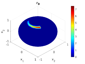
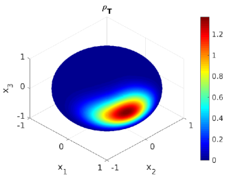
Figure 1: Initial, for $t=0$, (top), final, for $t=T$, (top) density $\rho_{T}$ and the corresponding control $u$ (bottom panel) after five iterations of the algorithm.

The initial control was taken to be constant, $u^{0}\equiv 0.1$, with the cost $\mathcal{I}[u^{0}]\approx 0.88$. Computing the iterations of the proposed algorithms, the cost $\mathcal{I}$ was observed to decrease monotonically (as it is expected): $\approx$ 0.59, 0.49, 0.46, 0.44, 0.43 and then stagnating at a value $\approx 0.43$. Terminal density $\rho_{T}$ and the corresponding control $u$ computed after five iterations are shown in Fig. 1 (middle and bottom panels, respectively).

VI CONCLUSION

We finally stress that the suggested nonlocal algorithm generates a $\mathcal{I}$-monotone control sequence, and typically takes a few (2-5) iterations to reach an acceptable solution. Free of any intrinsic parametric optimization, the method can be a “lifeline” for computationally demanding problems (like the presented one), where the direct approach, as well as different versions of the gradient descent, become prohibitively expensive.

Although the proposed approach has a fairly wide scope of application, there are significant restrictions. For instance, the concept of flat derivative (and, as a consequence, intrinsic derivative) does not apply to functionals $F:\,\mathcal{P}_{c}\to\mathbb{R}$ that are undefined ($=+\infty$) for measures, singular w.r.t. some reference one (typically, $\mathcal{L}^{n}$); this makes it impossible to treat several useful performance criteria such as entropy functionals of the Kullback-Leibler type [9].

-A Proof of Theorem 1

Let $t\mapsto\mu_{t}$ and $t\mapsto\bar{\mu}_{t}$ denote the weak solutions of the PDE (5) with initial condition $\mu_{0}=\vartheta$, corresponding to control inputs $u$ and $\bar{u}$, respectively. Recall that $\mu_{t}=(X_{0,t})_{\sharp}\vartheta$, $\bar{\mu}_{t}=(\bar{X}_{0,t})_{\sharp}\vartheta,$ and $X_{s,s}=\bar{X}_{s,s}=\mathop{\bf id}$ $\forall s\in\mathbb{R},$ where $X$ and $\bar{X}$ are the corresponding characteristic flows.

Denote $\mathcal{F}_{t}\doteq\bar{X}_{t,T}\circ X_{0,t}$. Since the map $x\mapsto\mathcal{F}_{t}(x)$ is a composition of two bijections, it is invertible. Standard arguments from the ODE theory imply that under assumptions $(A_{1})$–$(A_{3})$, the maps $t\mapsto\bar{X}_{t,T}(x)$ and $t\mapsto X_{0,t}(x)$ are Lipschitz on $I$, for any $x\in\mathbb{R}^{n}$. Hence, for any $x\in\mathbb{R}^{n}$, the function $t\mapsto\mathcal{F}_{t}(x)$ is absolutely continuous on $I$ as a composition of Lipschitz maps; in particular it is $\mathcal{L}^{1}$-a.e. differentiable: $\mathcal{F}_{t+\lambda}=\mathcal{F}_{t}+\lambda\,\partial_{t}\mathcal{F}_{t}+o(\lambda)\approx(\mathop{\bf id}+\lambda\,\partial_{t}\mathcal{F}_{t}\circ\mathcal{F}_{t}^{-1})\circ\mathcal{F}_{t}.$ Assumption $(A_{4})$ guarantees that, for any Borel measurable, locally bounded map $\varphi\colon\mathbb{R}^{n}\to\mathbb{R}^{n}$, the function $\lambda\mapsto\ell\left((\mathop{\bf id}+\lambda\mathcal{F})_{\sharp}\mu\right)$ is differentiable at zero, and $\displaystyle\frac{d}{d\lambda}\Big{|}_{\lambda=0}\ell\left((\mathop{\bf id}+\lambda f)_{\sharp}\mu\right)=\int D_{\mu}\ell(\mu)\cdot f\,d\mu$, where $D_{\mu}\ell$ stands for the intrinsic derivative. Thus,

$$\partial_{t}\ \ \ell\left(\left(\mathcal{F}_{t}\right)_{\sharp}\vartheta\right)=$$

$$=\ \ \frac{d}{d\lambda}\Big{|}_{\lambda=0}\ell\left(\left(\mathcal{F}_{t+\lambda}\right)_{\sharp}\vartheta\right)$$

$$=\ \ \frac{d}{d\lambda}\Big{|}_{\lambda=0}\ell\left(\left(\mathop{\bf id}+\lambda\,\partial_{t}\mathcal{F}_{t}\circ\mathcal{F}_{t}^{-1}\right)_{\sharp}\big{(}\left(\mathcal{F}_{t}\right)_{\sharp}\vartheta\big{)}\right)$$

$$=\ \ \int D_{\mu}\ell\left(\left(\mathcal{F}_{t}\right)_{\sharp}\vartheta\right)\cdot\partial_{t}\mathcal{F}_{t}\circ\mathcal{F}_{t}^{-1}\,d{\big{(}\left(\mathcal{F}_{t}\right)_{\sharp}\vartheta\big{)}}$$

$$=\ \ \int D_{\mu}\ell\big{|}_{\left(\bar{X}_{t,T}\circ X_{t}\right)_{\sharp}\vartheta}\circ\left(\bar{X}_{t,T}\circ X_{0,t}\right)\cdot$$

$$\qquad\partial_{t}(\bar{X}_{t,T}\circ X_{0,t})\,d\vartheta.$$ (22)

In the last expression, the partial derivative in $t$ is represented by the chain rule as

$$\partial_{t}(\bar{X}_{t,T}\circ X_{0,t})=\left[\partial_{\tau}\bar{X}_{t,T}\circ X_{0,\tau}+\partial_{\tau}\bar{X}_{\tau,T}\circ X_{0,t}\right]\big{|}_{\tau=t},$$

where $\partial_{\tau}\big{|}_{\tau=t}\bar{X}_{t,T}\circ X_{0,\tau}=\left(D_{x}\bar{X}_{t,T}\,V_{t}\right)\circ X_{0,t}\doteq\left(\bar{J}_{t,T}\,V_{t}\right)\circ X_{0,t}$ by direct computation, and $\partial_{\tau}\big{|}_{\tau=t}\bar{X}_{\tau,T}=-\bar{J}_{t,T}\,\bar{V}_{t}$ by (15). Plugging these expressions to (22), we obtain

$$\partial_{t}\ell\left(\left(\mathcal{F}_{t}\right)_{\sharp}\vartheta\right)\doteq \ \int\Big{[}D_{\mu}\ell^{*}\big{|}_{\left(\bar{X}_{t,T}\circ X_{t}\right)_{\sharp}\vartheta}\circ\bar{X}_{t,T}$$

$$\qquad\bar{J}_{t,T}(V_{t}-\bar{V}_{t})\Big{]}\circ X_{0,t}\,d\vartheta.$$ (23)

Now, the cost increment is represented as follows:

$$\Delta_{u}\mathcal{I}[\bar{u}] \doteq\ell(\mu_{T})-\ \ell(\bar{\mu}_{T})$$

$$=\ell\left((\bar{X}_{T,T}\circ X_{0,T})_{\sharp}\vartheta\right)-\ell\left((\bar{X}_{T,T}\circ\bar{X}_{0,T})_{\sharp}\vartheta\right)$$

$$-\underbrace{\left[\ell\left((\bar{X}_{0,T}\circ X_{0,0})_{\sharp}\vartheta\right)-\ell\left((\bar{X}_{0,T}\circ\bar{X}_{0,0})_{\sharp}\vartheta\right)\right]}_{\text{$\equiv 0$}}$$

$$=\int_{0}^{T} \!\!\partial_{t}\big{[}\ell\left((\bar{X}_{t,T}\circ X_{0,t})_{\sharp}\vartheta\right)-\ell\left((\bar{X}_{t,T}\circ\bar{X}_{0,t})_{\sharp}\vartheta\right)\big{]}\,dt.$$

By the semigroup property, $\bar{X}_{t,T}\circ\bar{X}_{0,t}=\bar{X}_{0,T}$, which implies that the second term under the sign of the time derivative in the latter expression is, in fact, independent of $t$, and therefore, $\Delta_{u}\mathcal{I}[\bar{u}]$ equals

$$\int_{0}^{T}\partial_{t}\ell\left(\left(\bar{X}_{t,T}\circ X_{0,t}\right)_{\sharp}\vartheta\right)\,dt=\int_{0}^{T}\partial_{t}\ell\left(\left(\mathcal{F}_{t}\right)_{\sharp}\vartheta\right)\,dt.$$

To complete the proof, it remains to combine the latter expression with (23) and use the representation formula $\mu_{t}=(X_{0,t})_{\sharp}\vartheta$.

References

- [1] J.-S. Li and N. Khaneja, “Ensemble control of bloch equations,” IEEE Transactions on Automatic Control, vol. 54, no. 3, pp. 528–536, 2009.
- [2] ——, “Control of inhomogeneous quantum ensembles,” Phys. Rev. A, vol. 73, p. 030302, Mar 2006.
- [3] T. E. Skinner, T. O. Reiss, B. Luy, N. Khaneja, and S. J. Glaser, “Application of optimal control theory to the design of broadband excitation pulses for high-resolution NMR,” Journal of Magnetic Resonance, vol. 163, no. 1, pp. 8–15, 2003.
- [4] S. Conolly, D. Nishimura, and A. Macovski, “Optimal control solutions to the magnetic resonance selective excitation problem,” IEEE Transactions on Medical Imaging, vol. 5, no. 2, pp. 106–115, 1986.
- [5] B. Bonnard, O. Cots, S. J. Glaser, M. Lapert, D. Sugny, and Y. Zhang, “Geometric optimal control of the contrast imaging problem in nuclear magnetic resonance,” IEEE Transactions on Automatic Control, vol. 57, no. 8, pp. 1957–1969, 2012.
- [6] B. Bonnard, A. Jacquemard, and J. Rouot, “Optimal control of an ensemble of Bloch equations with applications in mri,” in 2016 IEEE 55th Conference on Decision and Control (CDC), 2016, pp. 1608–1613.
- [7] S. Wang and J.-S. Li, “Free-endpoint optimal control of inhomogeneous bilinear ensemble systems,” Automatica, vol. 95, pp. 306–315, 2018.
- [8] X. Chen, “Ensemble observability of bloch equations with unknown population density,” Automatica, vol. 119, p. 109057, 2020.
- [9] L. Ambrosio and G. Savaré, “Gradient flows of probability measures,” in Handbook of differential equations: evolutionary equations. Vol. III, ser. Handb. Differ. Equ. Elsevier/North-Holland, Amsterdam, 2007, pp. 1–136.
- [10] G. Cavagnari, A. Marigonda, K. T. Nguyen, and F. S. Priuli, “Generalized control systems in the space of probability measures,” Set-Valued and Variational Analysis, vol. 26, no. 3, pp. 663–691, 2018.
- [11] B. Bonnet, C. Cipriani, M. Fornasier, and H.-L. Huang, “A measure theoretical approach to the mean-field maximum principle for training neurodes,” 2021. [Online]. Available: https://arxiv.org/abs/2107.08707
- [12] M. Staritsyn, N. Pogodaev, R. Chertovskih, and F. L. Pereira, “Feedback maximum principle for ensemble control of local continuity equations: An application to supervised machine learning,” IEEE Control Systems Letters, vol. 6, pp. 1046–1051, 2022.
- [13] M. Staritsyn, N. Pogodaev, and F. L. Pereira, “Linear-quadratic problems of optimal control in the space of probabilities,” IEEE Control Systems Letters, vol. 6, pp. 3271–3276, 2022.
- [14] P. Cardaliaguet, F. Delarue, J.-M. Lasry, and P.-L. Lions, The Master Equation and the Convergence Problem in Mean Field Games, ser. Ann. Math. Stud. Princeton, NJ: Princeton University Press, 2019, vol. 201.
- [15] N. Pogodaev and M. Staritsyn, “Impulsive control of nonlocal transport equations,” Journal of Differential Equations, vol. 269, no. 4, pp. 3585–3623, 2020.
- [16] J.-S. Li, I. Dasanayake, and J. Ruths, “Control and synchronization of neuron ensembles,” IEEE Transactions on Automatic Control, vol. 58, no. 8, pp. 1919–1930, 2013.
- [17] E. Zuazua, “Averaged control,” Automatica, vol. 50, no. 12, pp. 3077–3087, 2014.
- [18] A. Bressan and B. Piccoli, Introduction to the mathematical theory of control, ser. AIMS Series on Applied Mathematics. American Institute of Mathematical Sciences (AIMS), Springfield, MO, 2007, vol. 2.
- [19] A. Agrachev and Y. Sachkov, Control Theory from the Geometric Viewpoint, ser. Control theory and optimization. Springer, 2004.
- [20] B. Bonnet and H. Frankowska, “Necessary optimality conditions for optimal control problems in Wasserstein spaces,” Applied Mathematics & Optimization, vol. 84, no. 2, pp. 1281–1330, Dec 2021.
- [21] A. Krasovskii and N. Krasovskii, Control Under Lack of Information, ser. Systems & Control: Foundations & Applications. Birkhäuser Boston, 2012.
- [22] B. Tahayori, L. Johnston, I. Mareels, and P. Farrell, “Novel insight into magnetic resonance through a spherical coordinate framework for the bloch equation,” in Progress in Biomedical Optics and Imaging - Proceedings of SPIE, vol. 7258, 02 2009.