Gated Compression Layers for Efficient Always-On Models

Abstract

Mobile and embedded machine learning developers frequently have to compromise between two inferior on-device deployment strategies: sacrifice accuracy and aggressively shrink their models to run on dedicated low-power cores; or sacrifice battery by running larger models on more powerful compute cores such as neural processing units or the main application processor. In this paper, we propose a novel Gated Compression layer that can be applied to transform existing neural network architectures into Gated Neural Networks. Gated Neural Networks have multiple properties that excel for on-device use cases that help significantly reduce power, boost accuracy, and take advantage of heterogeneous compute cores. We provide results across five public image and audio datasets that demonstrate the proposed Gated Compression layer effectively stops up to 96% of negative samples, compresses 97% of positive samples, while maintaining or improving model accuracy.

1 Introduction

Advancements in lightweight architectures (Tan & Le, 2019), on-device libraries (David et al., 2021), and dedicated hardware accelerators have resulted in the ubiquitous deployment of machine learning models across millions of mobile, wearable, and smart devices. These advancements are powering a rapidly expanding category of on-device use-cases in Always-On computing. Always-On models are deployed today across millions of mobile devices, smart watches, fitness trackers, earbuds, smart doorbells, and beyond to enable use cases as broad as speaker detection; user authentication; activity recognition; noise reduction; fall detection; music classification; fault prevention; earthquake prediction; accident alerting; and more.

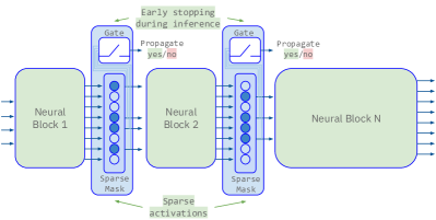
Figure 1: The proposed Gated Compression layer. One or more layers can be added to existing architectures to transform any network into an efficient Always-On Gated Neural Network.

Always-on models run continually, searching for potential signals of interest in a continuous stream of unsegmented sensor data. We refer to signals of interest as positive samples, with generic background data containing no signal of interest as negative samples. In real-world data, positive samples can be sporadic, hidden in an overwhelming negative data stream. A user might speak a few keywords a day; perform an activity multiple times per week; while the majority of users ideally never experience rare events like serious accidents. This exposes the main challenge with Always-On models - they are always on, continually searching for potential events; yet the events are sparse.

While modern mobile devices and wearables contain dedicated heterogeneous hardware to support running lightweight models at low power, its not enough to support the orders of magnitude increase in diversity and complexity of future use cases. Consumers desire more extensive and helpful experiences from their devices, while simultaneously expecting longer battery life and reduced climate impact. To fundamentally address this problem we need to think differently. We need machine learning techniques that enable us to move from an Always-On paradigm, to context aware models that only run when needed. Moreover, as model size continues to grow, we need options that enable larger context-aware models to be efficiently distributed across the multiple heterogeneous computing cores that are available in today’s modern devices (e.g. Always-On accelerators, DSPs, Neural cores, …). This enables much larger models to be run that can fit on any one processor, with the front-end of the model to run on extremely low-power Always-On accelerators to efficiently detect potential signals of interest and later stages of the model running on more compute-intensive processors only being triggered when appropriate.

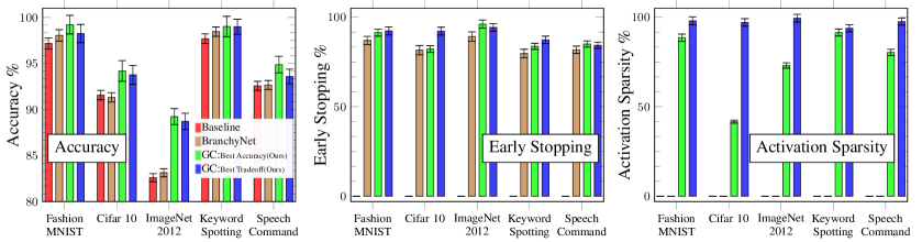
Figure 2: The proposed GC layer and two baseline techniques applied to five image and audio benchmark datasets. The GC $\alpha$, $\beta$ parameters enable models to be tuned to tradeoff accuracy vs early stopping vs compression based on the target use case requirements.

In this paper, we present a novel Gated Compression (GC) layer that can be applied to existing deep neural network architectures to transform any standard network into a Gated Neural Network. GC layers have the following important properties:

• Early Stopping: GC layers provide early stopping during inference. GC layers can be strategically placed throughout a network to immediately stop propagation of data when there is no signal of interest, significantly reducing compute and power. GC layers are jointly optimized during training to maximize early stopping, while not degrading accuracy or other key metrics;

• Activation Sparsity: GC layers automatically learn to compress intermediate feature data via activation sparsity to minimize the positive data that is propagated through an active network. Reducing feature dimensionality is key in heterogeneous computing systems due to the high cost of data transfer;

• Distributed Models: GC layers provide natural delimiters to enable large-scale models to be split and distributed over multiple compute islands on a single device, or potentially multiple devices and the cloud - while still running at low power due to early stopping and layer compression;

• Holistic Optimization: GC layers allow joint optimization of true positive detections while minimizing false positives errors. Multiple GC layers can be added to a single network if needed, which we show increases true positive detections while suppressing false positives.

The contributions of this paper are as follows:

• We propose a new Gated Compression layer and present an effective loss function that enables on-device models to be explicitly fine-tuned to specify the importance of early stopping, activation sparsity to reduce data transfer through the model, and boost overall model performance;

• We show how combing the gating and compression components in one layer improves all metrics over independent gating or compression.

• Furthermore, we show the performance impact of both the position and number of GC layers with a number of common model architectures finding that gating and compression can be improved with multiple gates cascaded through a network;

• We demonstrate through extensive experiments across 5 public image and audio datasets that various deep neural network models can be extended with Gated Compression layers to achieve up to 96% early stopping while also boosting accuracy (see Figure 2).

2 GC Layers for Always-On Models

For Always-On use cases involving ML models on low-power compute cores, by reducing the data transmission and computation needs, we can improve power efficiency, battery life and resource utilization while maintaining or improving accuracy. We present three core ideas in this paper to improve the efficiency of Always-On models: (i) Gated/Early Stopping: minimizing the number of negative samples propagated through a network by adding gates to stop unnecessary data transmission and computation; (ii) Activation Compression: minimizing the amount of positive samples propagated through a network at key bottleneck layers; (iii) Distributed Models: distributing a larger high-performance model over multiple heterogeneous compute stages across one or even multiple devices.

We first outline the framework to facilitate the introduction of the core ideas. A deep neural network, which consists of a chain of layers that are processed sequentially, can be split into smaller networks. The same results can be obtained by invoking the smaller networks sequentially. More specifically, a network $\mathcal{F}$ can be split into $k$ disjoint smaller networks $\mathcal{F}=\{\mathcal{F}^{i}\}_{i=1}^{k},$ such that $\mathcal{F}^{i}$ consumes the output of $\mathcal{F}^{i-1}$ and produces the input for $\mathcal{F}^{i+1}$. The input $x_{i}$ and output $y_{i}$ of the $i$-th smaller network $\mathcal{F}^{i}$ can be written as:

$$\begin{matrix}x_{i}&=&\left\{\begin{matrix}x&i=1\\ \mathcal{F}^{1\mapsto i-1}\left(x\right)&i>1\end{matrix}\right.\\[6.0pt] y_{i}&=&\mathcal{F}^{i}\left(x_{i}\right)\hskip 8.0pt=\hskip 8.0pt\mathcal{F}^{1\mapsto i}\left(x\right)\end{matrix},$$

$$\text{where\ \ \ }\mathcal{F}^{i\mapsto j}\left(\cdot\right)=\mathcal{F}^{j}\left(\mathcal{F}^{j-1}\left(\cdots\mathcal{F}^{i}\left(\cdot\right)\cdots\right)\right).$$

2.1 Gated/Early Stopping

In Always-On use cases, where the data stream is often dominated by negative samples, it is more efficient to early stop the transmission and computation of negative samples rather than processing them end-to-end. By early stopping, the data transmission and computations on later smaller networks can be skipped without degrading the performance.

Similar to the branch exit in BranchyNet (Teerapittayanon et al., 2016), a gate $\mathcal{G}^{i}$ is designed to stop data transmission and computation in any subsequently smaller network $\mathcal{F}^{j},\forall j\in(i,k]$. The gate $\mathcal{G}^{i}$, which is a binary gate, can be trained together with $\{\mathcal{F}^{m}\}_{m=1}^{i}$ to minimize the gate loss:

$$\mathcal{L}_{\text{gate}}^{i}(x,y)=\mathcal{L}\left(\mathcal{G}^{i}\left(\mathcal{F}^{1\mapsto i}\left(x\right)\right),\Omega^{i}(y)\right),$$ (1)

where $\mathcal{L}(\cdot,\cdot)$ is a loss function (e.g. cross entropy), and $\Omega^{i}(\cdot)$ is a predefined, problem-specific class mapping function for determining interesting classes.

2.2 Activation Compression

In Always-On use cases, positive samples should always propagate through the network end-to-end. Two adjacent smaller networks are connected together and the internal feature/activation maps are transmitting through them. The data amount can be substantial and the data transmission may cross boundaries, such as processors or devices. Thus, the data transmission can consume a significant amount of power, especially in Always-On scenarios.

To reduce the amount of transmitted data for positive samples, this paper proposes a Compression layer $\mathcal{C}_{\varphi}:\mathbb{R}^{n}\mapsto\mathbb{R}^{n}$ to learn data compression:

$$y=x\circ\varphi,$$ (2)

where $x$, $\varphi$, and $y$ are the input, weight, and output, respectively. The notation ‘$\circ$’ represents element-wise product. As a linear transformation, adding this type of layer, the entire network can still be trained using end-to-end back-propagation.

A Compression layer $\mathcal{C}^{i}$, which acts as a bottleneck and a bridge between $\mathcal{F}^{i}$ and $\mathcal{F}^{i+1}$, can be trained together with $\{\mathcal{F}^{m}\}_{m=1}^{k}$ to minimize the compression loss:

$$\begin{split}\mathcal{L}_{\text{comp}}^{i}(x,y)=&\mathcal{L}\left(\mathcal{F}^{i+1\mapsto k}\left(\mathcal{C}^{i}\mathcal{F}^{1\mapsto i}\left(x\right)\right),y\right)+\\ &\beta\mathcal{L}_{\text{trans}}(\varphi),\end{split}$$ (3)

where $\mathcal{L}_{\text{trans}}(\cdot)$ is a sparsity regularization term (e.g. $\mathcal{L}_{1}$) applied to the weight matrix $\varphi$ to promote sparsity in the activation outputs. Thus, the compression rate is controlled by the hyperparameter $\beta$, which enables fine-grained control over the compression.

Inspired by the binarized neural networks (Courbariaux et al., 2016), the weight matrix of the Compression layer is binarized to reduce its parameter size for deploying. The use of binary weights provides a natural way to represent which dimensions should be compressed (0) and which should be passed through (1).

2.3 GC Layer

A Gate stops negative samples early, while a Compression layer minimizes the amount of transmitted data for positive samples. It is intuitive to combine them into a signal layer, and insert into an existing network to gain the benefit of both. Additionally, our experimental results show this combination is practically beneficial, as it improves the performance of each other further.

A GC layer, a combination of the Gate and Compression layers, is proposed to minimize the amount of transmitted data and computation required. Here, we assume that the Gate $\mathcal{G}$ takes the output of the Compression layer $\mathcal{C}$ as input. Theoretically, it can take other inputs as well. However, according to our experimental results, it is advantageous to take the output of $\mathcal{C}$: (a) the connection is within the GC layer, making the GC layer easier to integrate into an existing network; (b) the input is sparse, resulting in a smaller $\mathcal{G}$, (c) $\mathcal{G}$ performs better as all layers before it can be fine-tuned for better representation learning.

A GC layer, $\mathcal{GC}^{i}=\{\mathcal{G}^{i},\mathcal{C}^{i}\}$, which acts as both a bridge and a gate between $\mathcal{F}^{i}$ and $\mathcal{F}^{i+1}$. There are various strategies to train $\mathcal{G}^{i}$ and $\mathcal{C}^{i}$, but our experiments indicate that training them together end-to-end with the entire network yields the best performance. Therefore, the GC layer is trained together with $\{\mathcal{F}^{m}\}_{m=1}^{k}$ for minimizing the $\mathcal{L}_{\mathcal{GC}}^{i}$ loss:

$$\begin{split}\mathcal{L}_{\mathcal{GC}}^{i}(x,y)=&\alpha\underbrace{\mathcal{L}\left(\mathcal{G}^{i}\left(\mathcal{C}^{i}\mathcal{F}^{1\mapsto i}\left(x\right)\right),\Omega^{i}(y)\right)}_{\textup{\tiny \leavevmode\hbox to6.15pt{\vbox to6.15pt{\text{[drawing]}}}Gate Loss}}+\\ &\beta\underbrace{\mathcal{L}_{\text{trans}}(\varphi)}_{\textup{\tiny \leavevmode\hbox to6.15pt{\vbox to6.15pt{\text{[drawing]}}}Trans. Cost}}+\\ &\eta\underbrace{\mathcal{L}\left(\mathcal{F}^{i+1\mapsto k}\left(\mathcal{C}^{i}\mathcal{F}^{1\mapsto i}\left(x\right)\right),y\right)}_{\textup{\tiny \leavevmode\hbox to6.15pt{\vbox to6.15pt{\text{[drawing]}}}Final Prediction Loss}}\end{split},$$

where $\alpha_{i}$ and $\beta_{i}$ control the early stopping and compression performance of the GC layer, respectively. The wieght $\eta$ is for the final prediction loss.

Implicit Pre-Training and Feature Selection. Besides enhancing power efficiency and resource utilization, our experiments also show that GC layers improve accuracy. This is due to the following: (1) The Gate guides the early layers towards a more favorable direction, similar to pre-training, and enables for early stopping of negative samples, allowing later layers to focus on positive samples; (2) The Compression layer discards irrelevant or partially relevant dimensions, similar to feature selection; (3) The GC layer, which combines the Gate and Compression layers, enhances the network efficiency and regularizes it to prevent overfitting.

2.4 Objective Function

Let $(x,y)$ be a data pair drawn from a distribution $\mathbf{P}(\mathbb{X},\mathbb{Y})$, where $x\in\mathbb{X}$ is a sample in $\mathbb{R}^{n}$ and $y\in\mathbb{Y}$ is the label in $\mathbb{N}$. Given a set of data pairs $\mathbf{D}(\mathbb{X},\mathbb{Y})=\{(x_{i},y_{i})|(x_{i},y_{i})\sim\mathbf{P}(\mathbb{X},\mathbb{Y})\}_{i=0}^{N}$, the goal is to learn the parameters $\theta\in\Theta$ of a deep neural network, $\mathcal{F}_{\theta}:\mathbb{X}\mapsto\mathbb{Y}$, that predicts the label $y$ for $\forall x\in\mathbf{D}(\mathbb{X})$ by solving:

$$\theta^{*}=\mathop{\mathrm{argmin}}\limits_{\theta\in\Theta}\underbrace{\underset{{{(x,y)\in\mathbf{D}}}(\mathbb{X},\mathbb{Y})}{{{{{{{\mathbb{E}}}}}}}}\mathcal{L}\left(\mathcal{F}_{\theta}(x),y\right)}_{\textup{\tiny Prediction loss}}+\xi\underbrace{\gamma(\theta)}_{\textup{\tiny Penalty}},$$

where $\gamma(\cdot)$ is the penalty term aiming at controlling the size and structure of the network $\mathcal{F}_{\theta}$. The weight $\xi$ controls the strength of the penalty term.

An existing network can be split into a set of smaller networks, $\widetilde{\mathcal{F}}_{\psi}=\left\{\mathcal{F}^{i},\mathcal{GC}^{i}\right\}_{i=1}^{k-1}\cup\left\{\mathcal{F}^{k}\right\}$ , by adding GC layers. The new network can be learned by solving:

$$\begin{split}\psi^{*}=&\mathop{\mathrm{argmin}}\limits_{\psi\in\Psi}\underset{{{(x,y)\in\mathbf{D}}}(\mathbb{X},\mathbb{Y})}{{{{{{{\mathbb{E}}}}}}}}\sum\limits_{i=1}^{k-1}\begin{bmatrix}\alpha_{i}\underbrace{\mathcal{L}_{\text{gate}}^{i}(x,y)}_{\textup{\tiny \leavevmode\hbox to6.15pt{\vbox to6.15pt{\text{[drawing]}}}Gate Loss}}+\\ \beta_{i}\underbrace{\mathcal{L}_{\text{\tiny trans}}^{i}({\varphi}_{\mathcal{C}}^{i})}_{\textup{\tiny \leavevmode\hbox to6.15pt{\vbox to6.15pt{\text{[drawing]}}}Trans. Cost}}\end{bmatrix}+\\ &\eta\underbrace{\mathcal{L}\left(\widetilde{\mathcal{F}}^{1\mapsto k}(x),y\right)}_{\textup{\tiny \leavevmode\hbox to6.15pt{\vbox to6.15pt{\text{[drawing]}}}Final Prediction Loss}}+\xi\underbrace{\gamma(\psi)}_{\textup{\tiny \leavevmode\hbox to6.15pt{\vbox to6.15pt{\text{[drawing]}}}Penalty}},\end{split}$$ (4)

$$\text{where \ \ \ }\mathcal{L}_{\text{gate}}^{i}(x,y) =\mathcal{L}\left(\mathcal{G}^{i}\left(\mathcal{C}^{i}\mathcal{F}^{1\mapsto i}\left(x\right)\right),\Omega^{i}(y)\right),$$

$$\widetilde{\mathcal{F}}^{i\mapsto j}(x) =\mathcal{C}^{j}\left(\mathcal{F}^{j}\widetilde{\mathcal{F}}^{i\mapsto j-1}(x)\right),$$

$$\eta =1-\sum_{i\in[1,k)}\alpha_{i}.$$

The ‘Gate Loss’ and ‘Final Prediction Loss’ are derived from classification error. To ensure balance in the classification loss, the weights ($\alpha_{i},\forall i\in[1,k)$ and $\eta$) are normalized so that their sum is equal to 1. The ‘Trans. Cost’ and ‘Penalty’ are regularization terms for the network structure, there are no strict constraints on their weights ($\beta_{i}$ and $\xi$).

The $\mathcal{L}_{\text{gate}}$ terms stop negative samples early, the $\mathcal{L}_{\text{trans}}$ terms minimize the amount of transmitted data for positive samples, and the ‘Final Prediction Loss’ term ensures the overall model performance. By training on all these terms together, the new network $\widetilde{\mathcal{F}}_{\psi}$ is optimized for better model performance and better power efficiency, battery life and resource utilization.

2.5 Distributed Model with GC Layers

For Always-On use cases, normally there are multiple heterogeneous compute islands available. For example, a sensor is connected to a microcontroller, then a sensor hub, a mobile device, and finally even the cloud.

GC layers can spit an existing network into smaller networks. This enables the execution of $\mathcal{F}^{i}$ on the $i$-th compute island, which in turn allows for the full utilization of all available resources. As a result, a larger and more powerful network can be built for better performance.

In the distributed scenario, two adjacent smaller networks $\mathcal{F}^{i}$ and $\mathcal{F}^{i+1}$ are running on different compute islands, and $\mathcal{F}^{i+1}$ takes the output of $\mathcal{F}^{i}$ as its input: $x_{i+1}\xleftarrow[\textsf{\tiny hardware boundaries}]{\textsf{\tiny Transmit across}}y_{i}.$ Since this data transmission crosses physical boundaries (e.g., device-to-device communication over Bluetooth or WiFi), it consumes a significant amount of power. This power consumption is amplified significantly for always-on use cases.

GC layers can create early exits and bottlenecks, which reduce the amount of data that needs to be transmitted across boundaries and decrease power consumption.

Table 1: Detailed Results of the Proposed GC Layer on Various Datasets.

	Dataset	Architecture	Method	$\alpha$	$\beta$	Accuracy	Early Stopping	Activation Sparsity
Image	Fashion MNIST	ResNet	Baseline	$\times$	$\times$	$0.97183\pm 0.00145$	$0\%$	$0\%$
			BranchyNet	$\times$	$\times$	$0.98051\pm 0.00623$	$87.03\%$	$0\%$
			With $\mathcal{G}$ only	$0.50$	$\times$	$0.98108\pm 0.00182$	$93.36\%$	$0\%$
			With $\mathcal{C}$ only	$\times$	$0.55$	$0.97998\pm 0.01406$	$0\%$	$98.07\%$
			With $\mathcal{GC}$:Best Trade-off	$0.50$	$0.55$	$0.98255\pm 0.00160$	$92.35\%$	$98.02\%$
			With $\mathcal{GC}$:Best Accuracy	$0.05$	$0.10$	$\boldsymbol{0.99219\pm 0.00091}$	$91.37\%$	$88.61\%$
	Cifar10	ResNet	Baseline	$\times$	$\times$	$0.90235\pm 0.00920$	$0\%$	$0\%$
			BranchyNet	$\times$	$\times$	$0.91312\pm 0.00508$	$81.57\%$	$0\%$
			With $\mathcal{G}$ only	$0.55$	$\times$	$0.92254\pm 0.00216$	$87.5\%$	$0\%$
			With $\mathcal{C}$ only	$\times$	$0.05$	$0.93962\pm 0.00586$	$0\%$	$42.10\%$
			With $\mathcal{GC}$:Best Trade-off	$0.70$	$0.8$	$0.93766\pm 0.06124$	$92.23\%$	$97.07\%$
			With $\mathcal{GC}$:Best Accuracy	$0.60$	$0.15$	$\boldsymbol{0.94187\pm 0.00244}$	$82.17\%$	$41.64\%$
	ImageNet 2012	ResNeXt	Baseline	$\times$	$\times$	$0.82591\pm 0.01085$	$0\%$	$0\%$
			BranchyNet	$\times$	$\times$	$0.83130\pm 0.00434$	$89.23\%$	$0\%$
			With $\mathcal{G}$ only	$0.25$	$\times$	$0.84316\pm 0.01262$	$95.66\%$	$0\%$
			With $\mathcal{C}$ only	$\times$	$0.35$	$0.84095\pm 0.02134$	$0\%$	$97.84\%$
			With $\mathcal{GC}$:Best Trade-off	$0.35$	$0.15$	${0.88715\pm 0.02100}$	$94.26\%$	$94.38\%$
			With $\mathcal{GC}$:Best Accuracy	$0.45$	$0.05$	$\boldsymbol{0.89221\pm 0.01844}$	$96.17\%$	$73.03\%$
Audio	Keyword Spotting	ResNet	Baseline	$\times$	$\times$	$0.97695\pm 0.00218$	$0\%$	$0\%$
			BranchyNet	$\times$	$\times$	$0.98462\pm 0.00509$	$79.73\%$	$0\%$
			With $\mathcal{G}$ only	$0.45$	$\times$	$0.98875\pm 0.00124$	$91.56\%$	$0\%$
			With $\mathcal{C}$ only	$\times$	$0.20$	$0.98742\pm 0.00278$	$0\%$	$97.77\%$
			With $\mathcal{GC}$:Best Trade-off	$0.45$	$0.20$	$0.98988\pm 0.00133$	$87.36\%$	$93.84\%$
			With $\mathcal{GC}$:Best Accuracy	$0.30$	$0.10$	$\boldsymbol{0.99018\pm 0.00164}$	$83.72\%$	$91.46\%$
	Speech Command	Inception	Baseline	$\times$	$\times$	$0.92527\pm 0.00876$	$0\%$	$0\%$
			BranchyNet	$\times$	$\times$	$0.92662\pm 0.00489$	$81.83\%$	$0\%$
			With $\mathcal{G}$ only	$0.05$	$\times$	$0.94111\pm 0.00932$	$94.26\%$	$0\%$
			With $\mathcal{C}$ only	$\times$	$0.35$	$0.93164\pm 0.00394$	$0\%$	$99.03\%$
			With $\mathcal{GC}$:Best Trade-off	$0.05$	$0.35$	$0.93590\pm 0.00411$	$84.31\%$	$97.53\%$
			With $\mathcal{GC}$:Best Accuracy	$0.25$	$0.10$	$\boldsymbol{0.94879\pm 0.00181}$	$85.03\%$	$80.36\%$

Overall, GC layers can be used to optimize existing networks for Always-On use cases, by reducing power consumption, boosting accuracy, and utilizing heterogeneous compute islands. These optimizations are obtained by creating early exits and bottlenecks, which minimize the amount of computation and data transfer required, allowing the network to run more efficiently in Always-On scenarios.

3 Experiments

We apply GC layers to Always-On scenarios across both image and audio classification tasks. In this section, we first describe the datasets, evaluation protocols, and implementation details used to train and test each model, then discuss results. We then ablate key components of the GC layer and discuss key insights.

3.1 Datasets, Architectures, and Evaluation Protocols

Despite the ubiquitous nature of Always-On computing in today’s consumer devices, there are limited public datasets that represent the true distribution of positive vs negative samples found in real-world use cases. Thankfully, common machine learning datasets such as ImageNet 2012 (Russakovsky et al., 2015) can be transformed into Always-On benchmark dataset by mapping a subset of labels to a generic negative class as a proxy for real-world background data.

For our experiments, we selected three common public image datasets: Fashion MNIST (Xiao et al., 2017), Cifar10 (Krizhevsky, 2009), and ImageNet 2012 (Russakovsky et al., 2015); and two public audio datasets: Keyword Spotting V2 (Leroy et al., 2019) and Speech Command (Warden, 2018). For each image dataset, we map every-other class to a generic background class to reflect an Always-On use case. All examples with even class labels are kept as positive examples, with all examples with odd class labels being mapped to a generic negative class. For example, in Cifar10 the even classes (airplane, bird, cat, deer, frog, ship) are unmodified while the odd classes (automobile, cat, dog, horse, truck) are grouped into a generic negative class. This simulates a 1:1 ratio between positive and negative samples. The audio datasets contain a pre-existing background class with a 1:9 ratio between positive and negative samples and required no additional class-label remapping. Note that real-world use cases can have a significant imbalance weighted towards negative samples, which only amplifies the need for techniques that support early stopping in Always-On models.

We use the following reference architectures for each dataset to demonstrate that GC layers can be applied to common model architectures (Figure 9): ResNets (He et al., 2016) (Fashion MNIST, Cifar10, Keyword Spotting); ResNeXt (Xie et al., 2017) (ImageNet 2012); and Inception (Szegedy et al., 2015) (Speech Command).

We evaluate the accuracy vs early-stopping performance of architectures expanded with GC layers. Early stopping is defined as the percentage of negative test examples that are successfully gated by the model without having to propagate to the final classification layer.

We compare architectures expanded with GC layers against two baseline architectures: a baseline architecture with no gating and a baseline architecture that employs the popular BranchyNet gating technique (Teerapittayanon et al., 2016). For each dataset, the baseline architecture, BranchyNet architecture, and GC architecture are identical with the exception of the additional BranchyNet or GC layer. We first report the results of a single gate placed at 40% within the depth of each network on the various image and audio test datasets. We then explore the impact of the position and number of gates, along with $\alpha,\beta$ tuning to achieve the best trade-off vs best-accuracy in the ablation studies.

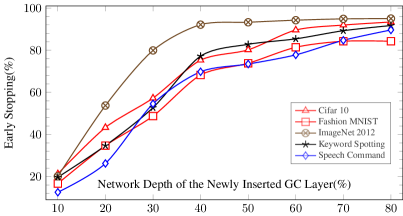
Figure 3: The Effect of Changing the Network Depth of A Newly Added GC Layer on Early Stopping Performance.

3.2 Implementation Details

All methods are implemented with TensorFlow 2.x (Abadi et al., 2015). Unless otherwise specified, the batch size is set to 512 and the training epoch is set to 200; the Adam (Kingma & Ba, 2015) optimizer with a fixed learning rate (0.01) is used for model training. As the larger ResNeXt-101 64x4d (Xie et al., 2017) was used for the ImageNet dataset, a larger batch size of 1536, training epoch of 100, and learning rate of 0.006 was used to reduce training time.

For prepossessing, the audio signals are converted into Mel-frequency cepstral coefficients, prior to input to the audio ResNet or Inception models. All experiments are repeated 10 times with the mean and variance results reported.

3.3 Accuracy vs Early Stopping Results

Figure 2 shows the results comparing the baseline models, BranchyNet models, and GC models across the image and audio datasets. Note that the ‘GC:Best Accuracy’ models consistently achieve the highest accuracy with competitive early stopping performance. On the other hand, the ‘GC:Best Tradeoff’ models achieve improved accuracy over both BranchyNet and the reference baseline across all datasets, ranging from an improvement of 1.06 percentage points (Fashion MNIST) to 6.12 percentage points (ImageNet) over the baseline architecture. Furthermore, they also have significantly improved early stopping performance over BranchyNet, with a range of 82.17% (Cifar 10) to 96.17% (ImageNet). Additionally, the GC models provide additional compression on the layer activation of the GC layer, reducing the feature dimensionality of any data that is transmitted to the next stage of the model, ranging from 41.64% (Cifar 10) to 97.53% (Speech Command).

The results in Figure 2 demonstrate that our GC layer can effectively identify and stop negative samples early, while simultaneously boosting model accuracy.

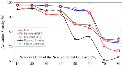
Figure 4: The Effect of Changing the Network Depth of A Newly Added GC Layer on Activation Sparsity.

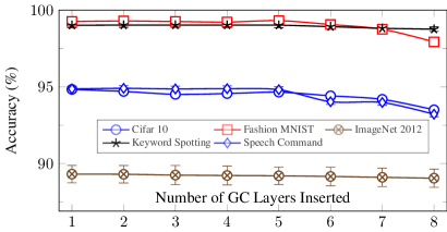
Figure 5: The Effect of Changing Number of GC Layers Inserted on Model Accuracy.

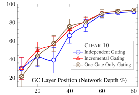
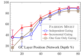
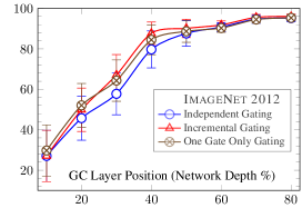
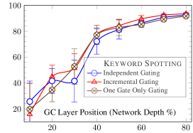
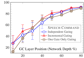
Figure 6: The Effect of Adding Multiple GC Layers on Early Stopping (%).

3.4 Best Trade-off vs Best Accuracy

On-device models need to carefully balance key metrics, such as accuracy, against critical factors, such as power usage or memory constraints. To reflect this real-world prioritization, we use the GC $\alpha$ and $\beta$ parameters to train two variants of models, one weighted towards achieving the best-possible accuracy (GC:Best Accuracy) the second weighted towards achieving the best-possible accuracy-vs-early-stopping compromise (GC:Best Tradeoff).

The results in Table 1 indicate that adding GC layers improves both accuracy and early stopping/compression performance. Specifically, ‘GC:Best Accuracy’ models consistently achieve the highest accuracy, while ‘GC:Best Trade-off’ models always obtain the best activation sparsity by balancing accuracy with more aggressive early stopping and compression. Specifically, the ‘GC:Best Tradeoff’ models achieve activation sparsity ranging from 93.84% (Keyword Spotting) to 97.53% (Speech Command), while the ‘GC:Best Accuracy’ models achieve activation sparsity ranging from 41.64% (Cifar 10) to 91.46% (Keyword Spotting). Additionally, in either case, GC models consistently outperform the baseline and BranchyNet reference models in both accuracy and early stopping.

Overall, the results in Table 1 demonstrate that the GC layer can help improve the model accuracy further, while providing the benefits of early stopping and compression. Furthermore, depending on the use case’s requirements, the GC layer can be configured with its $\alpha$ and $\beta$ parameters to prioritize early stopping and/or compression, while maintaining a high level of accuracy with a slight decrease if required.

3.5 Impact of GC Layer Position

Section 3.3 demonstrates significant early stopping and activation compression when placing a single GC layer 40% deep within each model architecture. In this experiment, we evaluate the impact of the position of a single GC layer within the network.

Figure 3 shows adding a single GC layer in a network can effectively early stop negative samples, and the early stopping performance improves as the GC layer is moved to a deeper position: Inserting a GC layer at 10% network depth early stops $10\sim 40\%$ of negative samples, and positioning it at the 40% depth improves early stopping to $70\sim 90\%$. This is because placing at a deeper position allows for more layers before it to be fine-tuned for better early stopping performance.

Figure 4 shows that as the GC layer is moved to deeper positions, activation sparsity decreases. Placement at 40% depth achieves a high activation sparsity of $90\sim 98\%$, but at 80% depth results in a lower activation sparsity of $60\sim 78\%$. This is because, as the GC layer is placed in shallower positions, it can compress more dimensions due to the larger internal feature map size.

Overall, Figures 3 and 4 demonstrate that a single GC layer can provide early stopping and compression benefits when inserted at various depths. Specifically, as the GC layer is placed deeper in the network, the early stopping performance improves while the compression performance declines. This insight can inform the positioning when inserting a GC layer based on the use case’s requirements.

3.6 Impact of Multiple GC Layers

To evaluate the effect of increasing the number of GC layers on the models’ performance, a set of experiments have been performed by inserting different numbers of GC layers into the existing baseline networks. To distribute the GC layers evenly, a balanced approach is chosen to select their positions. For example, to insert 4 GC layers, they are placed at the 20%, 40%, 60%, and 80% network depths.

The results in Figure 5 show that the accuracy remains almost unchanged when the number of GC layers is less than 5. However, when the number of GC layers exceeds 5, there is a noticeable decrease in accuracy of less than 2 percentage points for the Speech Command, Fashion MNIST, and Cifar 10 datasets.

To evaluate the early stopping performance with multiple GC Layers, three methods are used for comparison: (1) Independent Gating: 8 GC layers are inserted into the baseline model for training, only the gate in the GC layer at the specified position is active during inference; (2) Incremental Gating: 8 GC layers are inserted into the baseline model for training, gates in GC layers after the specified position are disabled during inference; (3) One Gate Only Gating: Only one GC layer is inserted into the baseline model at the specified position for training and inference.

The results in Figure 6 show that using incremental gating with multiple GC layers improves the early stopping performance compared to using ‘independent gating’ and ‘one gate only gating’.

Overall, the results in Figures 5 and 6 demonstrate that inserting multiple GC layers into a single network can provide various benefits: (1) Improved Early Stopping: multiple GC layers can incrementally stop more negative samples; (2) Multi-Stage Activation Compression: the amount of transmitted data can be reduced further by compressing with GC layers at different positions; (3) Flexibility: the position and number of GC layers can be adjusted based on the use case’s requirements.

4 Related Work

Deep neural networks have shown superior performance in many computer vision and natural language processing tasks. Recently, an emerging amount of work is applying deep neural networks on resource constrained edge devices (Dhar et al., 2019).

Model compression is a popular approach for resource efficiency. The model size is compressed via techniques such as network pruning, vector quantization, distillation, hashing, network projection, and binarization (Görmez & Koyuncu, 2022b; Liu et al., 2020; Wang et al., 2019; Ravi, 2017; Courbariaux et al., 2016; Hinton et al., 2015; Han et al., 2015; Chen et al., 2015; Gong et al., 2014).

By reducing weights and connections, a lot of light weight architectures were proposed for edge devices: MobileNets v1 (Howard et al., 2017), v2 (Sandler et al., 2018) and v3 (Howard et al., 2019), SqueezeNet (Iandola et al., 2016) and SqueezeNext (Gholami et al., 2018), ShuffleNet (Zhang et al., 2018), CondenseNet (Huang et al., 2018), and the NAS generated MnsaNet (Tan et al., 2019). These new lightweight architectures reduce model size and resource requirements while retaining fairly good accuracy.

Quantization reduces model complexity by using lower or mixed precision data representation. There are huge amount of emerging studies exploring 16-bit or lower precision for some or all of numerical values without much degradation in the model accuracy (Cambier et al., 2020; Guo, 2018; Micikevicius et al., 2017; Judd et al., 2015; Wang et al., 2018).

Encouraging sparse structure of the model architecture is able to reduce model complexity. The group lasso regularization (Feng & Darrell, 2015; Lebedev & Lempitsky, 2016; Wen et al., 2016) and learnable dropout techniques (Boluki et al., 2020; Molchanov et al., 2017) are efficient ways to encourage sparse structures in various deep neural network components and weights.

To utilize resources across hardware boundaries, distributed deployment techniques have been proposed (Teerapittayanon et al., 2017; McMahan et al., 2017; Teerapittayanon et al., 2016; Tsianos et al., 2012; Ouyang et al., 2017; Gormez et al., 2022; Görmez & Koyuncu, 2022a; Kaya et al., 2019) to deploy deep neural network over multiple compute islands.

Our work is related to both distributed deployment and sparse structure. For better model performance, the proposed GC layer can distribute a single model across heterogeneous compute islands to fully utilize all resources available. To reduce the data transmission and computation needs, the GC layer allows early stopping for data with no signal of interest and minimizes the amount of transmitted data for other samples.

5 Conclusion

In this paper, we introduce a novel Gated Compression (GC) layer that can be incorporated into existing neural network architectures to convert them into Gated Neural Networks. This allows standard networks to benefit from the advantages of gating, such as improved performance and efficiency.

The GC layer is a lightweight layer for efficiently reducing the data transmission and computation needs. Its gate can (a) efficiently save the data transmission by early stopping the negative samples and (b) positively affect the model performance by (i) pre-training the early layers towards a better direction and (ii) simplifying the problem be removing negative samples early; Its Compression layer can (a) efficiently save the data transmission by compressing on its output of the remaining samples for propagating across boundaries and (b) positively affect the model performance by discarding irrelevant or partially relevant dimensions. Together, the GC layer is able to reduce the amount of transmitted data efficiency by early stopping $96\%$ of negative samples and compressing $97\%$ per propagated sample, while improving accuracy by $1.06\sim 6.12$ percentage points.

GC layers can be integrated into an existing network without modification. Then, the new network is able to be distributed across multiple heterogeneous compute islands to fully utilize all resources available. Therefore, larger and more powerful models can be built for better performance for Always-On use cases.

Appendix

Appendix A Property of the Distributed Framework

Proposition A.1.

The distributed framework will not affect the model prediction performance.

Proof.

For any raw input $x$, the same output of $\mathcal{F}_{\theta}$ can be produced with all $k$ disjoint sub models together:

$$\mathcal{F}_{\theta}(x)=\underbrace{\mathcal{F}^{k}\cdots\mathcal{F}^{1}}_{\texttt{\tiny$k$ sub models}}(x)=\mathcal{F}^{1\mapsto k}(x).$$

∎

Appendix B Metrics of Gated

To quantify and evaluate the performance of a Gate $\mathcal{G}$, a list of metrics are defined using True/False Positive/Negative ($TP$, $TN$, $FP$, and $FN$).

Definition B.1 (Stop Rate $\mathcal{P}_{sr}$).

The percentage of samples, which are stopped by a Gate, is defined as:

$$\mathcal{P}_{sr}=\frac{TP+FP}{TP+FP+TN+FN}.$$

Definition B.2 (Negative Pass Through Rate $\mathcal{P}_{nptr}$).

The percentage of negative samples, which are mistakenly allowed to pass through by a Gate, is defined as:

$$\mathcal{P}_{nptr}=\frac{FP}{FP+TN}.$$

Definition B.3 (Positive Lost Rate $\mathcal{P}_{plr}$).

The percentage of positive samples, which are mistakenly stopped by a Gate, is defined as:

$$\mathcal{P}_{plr}=\frac{FN}{FN+TP}.$$

Definition B.4 (Negative Correction Rate $\mathcal{P}_{ncr}$).

The percentage of negative samples, which are correctly stopped by a Gate $\mathcal{G}$ but will be incorrectly classified later if the Gate lets them propagate through, is defined as:

$$\mathcal{P}_{ncr}=\frac{\left|\left\{(x,y)|\mathcal{G}(x)=0\wedge\mathcal{F}(x)\neq 0\right\}\right|}{\left|\left\{(x,y)|y=0\right\}\right|}.$$

Remark.

A larger $\mathcal{P}_{ncr}$ is preferable since it decreases the difficulty for later sub models.

Appendix C Properties of Compression layer

Proposition C.1.

The Compression layer has the following property: a sparse weight matrix $\varphi$ leads to a sparse output $y$.

Corollary C.1.

For a Compression layer, encouraging the sparsity of $y$ is equivalent to putting a sparsity regularization on $\varphi$.

Definition C.1 (Dropout Rate $\mathcal{P}_{dr}$).

The percentage of output dimensions, which are dropped out by a Compression layer, is defined as:

$$\mathcal{P}_{dr}(\mathcal{C}_{\varphi})=1-\frac{|\varphi|_{0}}{\dim\varphi}.$$

Appendix D Binarizing the Weight Matrix

To push most dimensions of the weight matrix $\varphi$ toward $\{0,1\}$, we apply weight clipping $\sigma(\cdot)$ (Equation 5) to limit the domain. Specifically, we use the element-wised ReLU-1 (Krizhevsky & Hinton, 2010) activation function for constraining all dimensions into the range of $[0,1]$.

$$\sigma(\varphi)=\text{min}(1,\text{max}(0,\varphi))$$ (5)

During the forward propagation, the binarize function, defined in Equation 6, is used for converting a floating weight into a binary weight.

$$\Gamma(\varphi)=\mathbf{1}_{{\varphi}>\frac{1}{2}},\forall\varphi\in[0,1]$$ (6)

Proposition D.1.

The Compression layer with binarized weight matrix has the following property: the sparsity of $y$ is controlled by the sparsity of $\Gamma(\varphi)$ instead of $\varphi$ itself.

Corollary D.1.

To yield sparse $\Gamma(\varphi)$ and $y$, $\mathcal{L}_{\text{trans}}$ (in Equation 3) could be $\mathcal{L}_{p},\forall p>0$.

Since $\mathcal{L}_{2}$ is smoother than $\mathcal{L}_{1}$ in the domain $\varphi\in[0,1]$, which yields better degree of control. Therefore, in this paper, we use $\mathcal{L}_{2}$ for the data transmission regularization. Figure 7 is an real example of weight distribution using $\mathcal{L}_{2}$ regularization.

Conjecture D.2.

Without regularization, the Compression layer with binarized weight matrix still encourages sparse output.

Proof.

During the forward propagation, all weight dimensions are binarized into $\{0,1\}$, therefore, the dimensions of $0$s will yield $0$s in the corresponding dimensions of the output (Proposition C.1).

Assuming all weight dimensions are drew from a Bernoulli distribution: $\varphi_{i}\sim\text{Bernoulli}(p),p\in(0,1),\forall i\in[0,\dim\varphi]$. Then, the expected sparsity is $(1-p)$, which is lager than $0$.

Additionally, our experiment results also confirm that there are about 40% sparsity in the activation outputs even without regularization. ∎

As shown in Equation 6 and Figure 8, the derivative of $\Gamma(\cdot)$ is: $\frac{\mathrm{d}\Gamma}{\mathrm{d}\varphi}=0,\forall\varphi\in[0,1]$. Therefore, it is impossible to do gradient back-propagating. Instead, the straight through estimator (Bengio et al., 2013; Courbariaux et al., 2016; Yin et al., 2019) is applied during back-propagation for estimating the gradient.

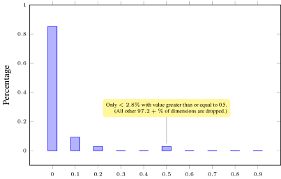
Figure 7: A real example of the weight distribution after 100 epochs on the Cifar10 dataset.

Appendix E Compactness of the Compression layer

Proposition E.1.

The Compression layer has the following property: By binarizing, the data amount of the weight matrix can be reduced by $N$ (number of bits required for one weight dimension in the default datatype) times for deploying.

Proof.

Once binarized, any dimension in $w$ can be represented with 1-bit ($\{0,1\}$) instead of a $N$-bits datatype (for example, in Tensorflow, the default datatype is float32, which is 32-bits). ∎

Additionally, the $\mathcal{L}_{\text{trans}}$ regularization (Equation 3) encourages sparse weight matrix, for which sparse encoding can reduce the size further.

Corollary E.1.

Let $m$ be the number of dimensions, $p$ be the percentage of the non-zero weights, and $N$ is the number of bits required for a weight in the default datatype, then the data compression rate of sparse encoding is

$$\mathcal{P}_{cr}(m,p)=\frac{N}{p\left\lceil\log_{2}(m)\right\rceil}.$$ (7)

Proof.

The number of bits required to encode the index of all $m$ is $\left\lceil\log_{2}(m)\right\rceil$, and there are $pm$ non-zero dimensions to be encoded. Therefore, the number of bits required for encoding all non-zero dimensions is $pm\left\lceil\log_{2}(m)\right\rceil$.

Without encoding, each weight is stored in $N$-bits, which in total equates to $Nm$ bits; With sparse encoding, the required bits are reduced from $Nm$ to $pm\left\lceil\log_{2}(m)\right\rceil$ , which yields a compression rate of $\frac{N}{p\left\lceil\log_{2}(m)\right\rceil}$. ∎

Normally, $p\leq 5\%$, $m\leq 2^{9}$ and $N=32$ from our experiment results. With Equation 7, we have $\mathcal{P}_{cr}(5\%,2^{9})={71}$. In total, its parameter size is ${32*2^{9}}/{71}=230.8$ bits (or ${2^{9}}/{71}=\textbf{7.2}$ float32), which is minimal and compact enough for edge hardware modules.

Appendix F Model Architecture

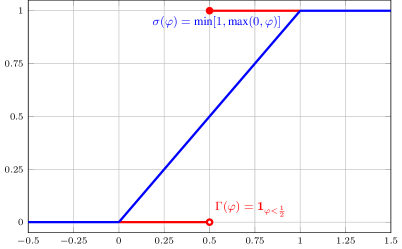
Figure 8: Plot of the Binarize Function $\Gamma(\cdot)$ and the Weight Clipping Function $\sigma(\cdot)$

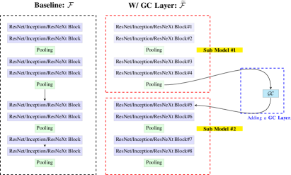
Figure 9: Model Architectures: the Baseline $\mathcal{F}$ model and the new $\widetilde{\mathcal{F}}$ model built from Baseline by adding one GC Layer. Note: (1) The model architectures consist of 8 ResNet/Inception/ResNeXt blocks, and additional 2 linear blocks for the classification head; (2) A GC layer can be inserted after each of these blocks.

Appendix G Deeper Analysis

A set of experiments on the Cifar10 dataset are performed to analyze the properties of the proposed GC layer deeper.

G.1 Effectiveness of $\mathcal{G}$

To evaluate the performance of the Gate $\mathcal{G}$, a set of experiments are conducted by varying its hyperparameter $\alpha$. To separate its impact from the Compression layer $\mathcal{C}$, the weight matrix of $\mathcal{C}$ is set to all 1s to deactivate it.

$\mathcal{G}$ Positively Affects the Model Performance. In Figure 10, for $\alpha\in[0.05,0.8]$, $\widetilde{\mathcal{F}}$ consistently performs better than Baseline with, which indicates that $\mathcal{G}$ can boost the performance of $\widetilde{\mathcal{F}}$. This may be contributed by 1) similar to pre-training, it may tune the early layers to a better direction; 2) it reduces false positives by stopping negative samples earlier.

Larger $\alpha$ Encourages Better $\mathcal{G}$. Figure 11 shows both positive lost rate ($\mathcal{P}_{plr}$) and negative pass through rate ($\mathcal{P}_{nptr}$) decrease along with the increase of $\alpha$. This aligns with our expectations as a larger $\alpha$ places more weight on $\mathcal{G}$ during training.

$\mathcal{G}$ Reduces Difficulty for $\widetilde{\mathcal{F}}$. Figure 11 shows that the negative corrected rate ($\mathcal{P}_{ncr}$) is always above 0, indicating that $\mathcal{G}$ decreases the complexity for $\widetilde{\mathcal{F}}$.

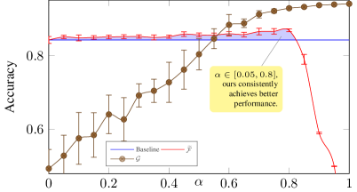
Figure 10: Effect of Changing $\alpha$ on $\widetilde{\mathcal{F}}$.

G.2 Gating Analysis

A gate can have a good early stopping performance for the negative samples, while incorrectly stopping a good percentage of positive samples at the same time. Therefore, it is important to analyze the gating performance to ensure that the majority of positive samples pass through the network end-to-end for the final classification or prediction task.

The results in Figure 12 show our GC models consistently outperform BranchyNet in gating performance, as shown by the AUC and ROC curves.

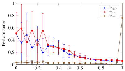
Figure 11: Effect of Changing $\alpha$ on $\mathcal{G}$.

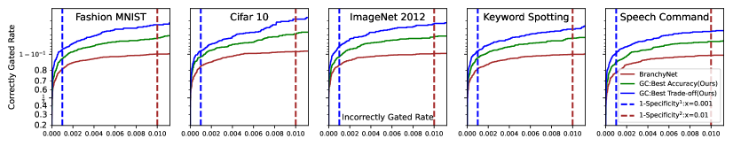
Figure 12: ROC Curves for Early Stopping Across All Five Datasets.

G.3 Effectiveness of $\mathcal{C}$

To understand the effectiveness of the Compression layer $\mathcal{C}$, a set of experiments are carried out by changing its hyperparameter $\beta$. To isolate it from the Gate $\mathcal{G}$, $\alpha$ is fixed at $0.5$. The results are reported in Figure 13.

$\mathcal{C}$ Encourages Sparsity Even without Regularization. When $\beta=0$, it still achieves the density of 0.579. This empirically confirms the Conjecture D.2.

$\mathcal{C}$ Efficiently Controls Activation Sparsity with $\beta$. A larger $\beta$ leads to a more sparse output. When $\beta=0.72$, it achieves density of 2.7% while maintaining the accuracy of 0.879. In another words, it allows for a 97.3% reduction in data transmission without compromising accuracy.

$\mathcal{C}$ Positively Affects the Model Performance. Similar to feature selection and dimensional reduction, the Compression layer improves and stabilizes the model performance by dropping irrelevant or partially relevant dimensions to avoid their negative impact on the model performance. When $\beta<0.72$, $\widetilde{\mathcal{F}}$ achieves $1\%\sim 4.5\%$ accuracy gain comparing to Baseline with the same $\alpha=0.5$.

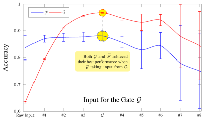
Figure 13: Effect of Changing $\beta$ on $\widetilde{\mathcal{F}}$.

G.4 Inputs for $\mathcal{G}$

From Figure 9, there are 8 ResNet/Inception/ResNeXt blocks, to understand the effect of the input layer of the Gate $\mathcal{G}$, a set of experiments are performed by linking its input to different layers. Based on the results in Table 1, the hyperparameters are chosen as $\alpha=0.7,\beta=0.6$. The results are reported in Figure 14.

Figure 14: Effect of Changing $\mathcal{G}$’s Input.

The Performance of $\mathcal{G}$ Increases Significantly along with the Movement of Placing $\mathcal{G}$ Closer to $\mathcal{C}$. This is expected as there are more layers to be tuned for better performance.

The Performance of $\widetilde{\mathcal{F}}$ Increases along with the Movement of Placing $\mathcal{G}$ Closer to $\mathcal{C}$. This aligns with our previous observation in relation to performance: a better $\mathcal{G}$ can also benefit $\widetilde{\mathcal{F}}$ to achieve better performance.

Additionally, placing the gate before $\mathcal{C}$ requires a larger $\mathcal{G}$ as the output of an early layer without compression or dropping tends to be larger. A possible workaround is adding additional pooling layers (for example, AvgPool, MaxPool, Conv1x1) to shrink the input. However, this gradually disengages $\mathcal{G}$ from $\widetilde{\mathcal{F}}$. Therefore, it decreases the pre-training benefit for $\widetilde{\mathcal{F}}$.

The Performances of Both $\widetilde{\mathcal{F}}$ and $\mathcal{G}$ Decrease Once $\mathcal{G}$ Is After $\mathcal{C}$. The reasons are: (1) the output of the later blocks after $\mathcal{GC}$ is designed to have way more channels that makes the input more noisy for $\mathcal{G}$; (2) the overlapping of $\widetilde{\mathcal{F}}$ and $\mathcal{G}$ is large, which leads to greater competition than cooperation.

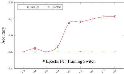
Figure 15: Two Stages Training Performances.

Overall, it is preferable to connect the input layer of $\mathcal{G}$ to the output from $\mathcal{C}$ since it generates the best performance for both $\widetilde{\mathcal{F}}$ and $\mathcal{G}$. Additionally, this also streamlines the implementation of the GC layer, as the connection is internal.

G.5 Manually Two Stages Training

In this section, we are exploring the difference between training $\mathcal{G}$ and $\widetilde{\mathcal{F}}$ end-to-end simultaneously versus manually training them in two stages and then merging together for inference. To simulate the two stages training schema, the gradient flow between the two sub-models is intentionally halted. Subsequently, we alternate between training $\mathcal{G}$ for $N$ epochs and $\widetilde{\mathcal{F}}$ for $N$ epochs, repeating this process until a total of 512 epochs are reached. When the number of epochs per training switch is $2^{8}$ (256), it forms a hierarchical ensemble model with two sub-models trained in sequence. The results are reported in Figure 15.

Disabling $\mathcal{C}$ Performs Slightly Better Than Enabling $\mathcal{C}$. $\mathcal{C}$ is added on purpose to drop less useful dimensions. Since the gradient is stopped between the two sub models, $\mathcal{C}$ is optimized for $\mathcal{G}$ only. The useful information for $\widetilde{\mathcal{F}}$ is further reduced when $\mathcal{C}$ is in effect. Moreover, the results suggest that simultaneously training all components end-to-end is more effective than a two-stage training approach, as the components can work together and optimize the overall performance.

References

- Abadi et al. (2015) Abadi, M., Agarwal, A., Barham, P., Brevdo, E., Chen, Z., Citro, C., Corrado, G. S., Davis, A., Dean, J., Devin, M., Ghemawat, S., Goodfellow, I., Harp, A., Irving, G., Isard, M., Jia, Y., Jozefowicz, R., Kaiser, L., Kudlur, M., Levenberg, J., Mané, D., Monga, R., Moore, S., Murray, D., Olah, C., Schuster, M., Shlens, J., Steiner, B., Sutskever, I., Talwar, K., Tucker, P., Vanhoucke, V., Vasudevan, V., Viégas, F., Vinyals, O., Warden, P., Wattenberg, M., Wicke, M., Yu, Y., and Zheng, X. TensorFlow: Large-scale machine learning on heterogeneous systems, 2015. URL http://tensorflow.org/. Software available from tensorflow.org.
- Bengio et al. (2013) Bengio, Y., Léonard, N., and Courville, A. C. Estimating or propagating gradients through stochastic neurons for conditional computation. CoRR, abs/1308.3432, 2013. URL http://arxiv.org/abs/1308.3432.
- Boluki et al. (2020) Boluki, S., Ardywibowo, R., Dadaneh, S. Z., Zhou, M., and Qian, X. Learnable bernoulli dropout for bayesian deep learning. arXiv preprint arXiv:2002.05155, 2020.
- Cambier et al. (2020) Cambier, L., Bhiwandiwalla, A., Gong, T., Nekuii, M., Elibol, O. H., and Tang, H. Shifted and squeezed 8-bit floating point format for low-precision training of deep neural networks. arXiv preprint arXiv:2001.05674, 2020.
- Chen et al. (2015) Chen, W., Wilson, J., Tyree, S., Weinberger, K., and Chen, Y. Compressing neural networks with the hashing trick. In International conference on machine learning, pp. 2285–2294. PMLR, 2015.
- Courbariaux et al. (2016) Courbariaux, M., Hubara, I., Soudry, D., El-Yaniv, R., and Bengio, Y. Binarized neural networks: Training deep neural networks with weights and activations constrained to+ 1 or-1. arXiv preprint arXiv:1602.02830, 2016.
- David et al. (2021) David, R., Duke, J., Jain, A., Janapa Reddi, V., Jeffries, N., Li, J., Kreeger, N., Nappier, I., Natraj, M., Wang, T., et al. Tensorflow lite micro: Embedded machine learning for tinyml systems. Proceedings of Machine Learning and Systems, 3:800–811, 2021.
- Dhar et al. (2019) Dhar, S., Guo, J., Liu, J., Tripathi, S., Kurup, U., and Shah, M. On-device machine learning: An algorithms and learning theory perspective. arXiv preprint arXiv:1911.00623, 2019.
- Feng & Darrell (2015) Feng, J. and Darrell, T. Learning the structure of deep convolutional networks. In Proceedings of the IEEE international conference on computer vision, pp. 2749–2757, 2015.
- Gholami et al. (2018) Gholami, A., Kwon, K., Wu, B., Tai, Z., Yue, X., Jin, P., Zhao, S., and Keutzer, K. Squeezenext: Hardware-aware neural network design. In Proceedings of the IEEE Conference on Computer Vision and Pattern Recognition Workshops, pp. 1638–1647, 2018.
- Gong et al. (2014) Gong, Y., Liu, L., Yang, M., and Bourdev, L. Compressing deep convolutional networks using vector quantization. arXiv preprint arXiv:1412.6115, 2014.
- Gormez et al. (2022) Gormez, A., Dasari, V. R., and Koyuncu, E. E2CM: Early exit via class means for efficient supervised and unsupervised learning. In 2022 International Joint Conference on Neural Networks (IJCNN), jul 2022.
- Guo (2018) Guo, Y. A survey on methods and theories of quantized neural networks. arXiv preprint arXiv:1808.04752, 2018.
- Görmez & Koyuncu (2022a) Görmez, A. and Koyuncu, E. Class based thresholding in early exit semantic segmentation networks, 2022a.
- Görmez & Koyuncu (2022b) Görmez, A. and Koyuncu, E. Pruning early exit networks, 2022b.
- Han et al. (2015) Han, S., Mao, H., and Dally, W. J. Deep compression: Compressing deep neural networks with pruning, trained quantization and huffman coding. arXiv preprint arXiv:1510.00149, 2015.
- He et al. (2016) He, K., Zhang, X., Ren, S., and Sun, J. Deep residual learning for image recognition. In Proceedings of the IEEE conference on computer vision and pattern recognition, pp. 770–778, 2016.
- Hinton et al. (2015) Hinton, G., Vinyals, O., and Dean, J. Distilling the knowledge in a neural network. In NIPS Deep Learning and Representation Learning Workshop, 2015. URL http://arxiv.org/abs/1503.02531.
- Howard et al. (2019) Howard, A., Sandler, M., Chu, G., Chen, L.-C., Chen, B., Tan, M., Wang, W., Zhu, Y., Pang, R., Vasudevan, V., et al. Searching for mobilenetv3. In Proceedings of the IEEE/CVF International Conference on Computer Vision, pp. 1314–1324, 2019.
- Howard et al. (2017) Howard, A. G., Zhu, M., Chen, B., Kalenichenko, D., Wang, W., Weyand, T., Andreetto, M., and Adam, H. Mobilenets: Efficient convolutional neural networks for mobile vision applications, 2017.
- Huang et al. (2018) Huang, G., Liu, S., Van der Maaten, L., and Weinberger, K. Q. Condensenet: An efficient densenet using learned group convolutions. In Proceedings of the IEEE conference on computer vision and pattern recognition, pp. 2752–2761, 2018.
- Iandola et al. (2016) Iandola, F. N., Han, S., Moskewicz, M. W., Ashraf, K., Dally, W. J., and Keutzer, K. Squeezenet: Alexnet-level accuracy with 50x fewer parameters and< 0.5 mb model size. arXiv preprint arXiv:1602.07360, 2016.
- Judd et al. (2015) Judd, P., Albericio, J., Hetherington, T., Aamodt, T., Jerger, N. E., Urtasun, R., and Moshovos, A. Reduced-precision strategies for bounded memory in deep neural nets. arXiv preprint arXiv:1511.05236, 2015.
- Kaya et al. (2019) Kaya, Y., Hong, S., and Dumitras, T. Shallow-deep networks: Understanding and mitigating network overthinking. In International conference on machine learning, pp. 3301–3310. PMLR, 2019.
- Kingma & Ba (2015) Kingma, D. P. and Ba, J. Adam: A method for stochastic optimization. In Bengio, Y. and LeCun, Y. (eds.), 3rd International Conference on Learning Representations, ICLR 2015, San Diego, CA, USA, May 7-9, 2015, Conference Track Proceedings, 2015. URL http://arxiv.org/abs/1412.6980.
- Krizhevsky (2009) Krizhevsky, A. Learning multiple layers of features from tiny images. Technical report, 2009.
- Krizhevsky & Hinton (2010) Krizhevsky, A. and Hinton, G. Convolutional deep belief networks on cifar-10. Unpublished manuscript, 40(7):1–9, 2010.
- Lebedev & Lempitsky (2016) Lebedev, V. and Lempitsky, V. Fast convnets using group-wise brain damage. In Proceedings of the IEEE Conference on Computer Vision and Pattern Recognition, pp. 2554–2564, 2016.
- Leroy et al. (2019) Leroy, D., Coucke, A., Lavril, T., Gisselbrecht, T., and Dureau, J. Federated learning for keyword spotting. In ICASSP 2019-2019 IEEE International Conference on Acoustics, Speech and Signal Processing (ICASSP), pp. 6341–6345. IEEE, 2019.
- Liu et al. (2020) Liu, J., Tripathi, S., Kurup, U., and Shah, M. Pruning algorithms to accelerate convolutional neural networks for edge applications: A survey. arXiv preprint arXiv:2005.04275, 2020.
- McMahan et al. (2017) McMahan, B., Moore, E., Ramage, D., Hampson, S., and y Arcas, B. A. Communication-efficient learning of deep networks from decentralized data. In Artificial Intelligence and Statistics, pp. 1273–1282. PMLR, 2017.
- Micikevicius et al. (2017) Micikevicius, P., Narang, S., Alben, J., Diamos, G., Elsen, E., Garcia, D., Ginsburg, B., Houston, M., Kuchaiev, O., Venkatesh, G., et al. Mixed precision training. arXiv preprint arXiv:1710.03740, 2017.
- Molchanov et al. (2017) Molchanov, D., Ashukha, A., and Vetrov, D. Variational dropout sparsifies deep neural networks. arXiv preprint arXiv:1701.05369, 2017.
- Ouyang et al. (2017) Ouyang, W., Wang, K., Zhu, X., and Wang, X. Chained cascade network for object detection. In Proceedings of the IEEE International Conference on Computer Vision, pp. 1938–1946, 2017.
- Ravi (2017) Ravi, S. Projectionnet: Learning efficient on-device deep networks using neural projections. arXiv preprint arXiv:1708.00630, 2017.
- Russakovsky et al. (2015) Russakovsky, O., Deng, J., Su, H., Krause, J., Satheesh, S., Ma, S., Huang, Z., Karpathy, A., Khosla, A., Bernstein, M., Berg, A. C., and Fei-Fei, L. ImageNet Large Scale Visual Recognition Challenge. International Journal of Computer Vision (IJCV), 115(3):211–252, 2015. doi: 10.1007/s11263-015-0816-y.
- Sandler et al. (2018) Sandler, M., Howard, A., Zhu, M., Zhmoginov, A., and Chen, L.-C. Mobilenetv2: Inverted residuals and linear bottlenecks. In Proceedings of the IEEE conference on computer vision and pattern recognition, pp. 4510–4520, 2018.
- Szegedy et al. (2015) Szegedy, C., Liu, W., Jia, Y., Sermanet, P., Reed, S., Anguelov, D., Erhan, D., Vanhoucke, V., and Rabinovich, A. Going deeper with convolutions. In Proceedings of the IEEE conference on computer vision and pattern recognition, pp. 1–9, 2015.
- Tan & Le (2019) Tan, M. and Le, Q. Efficientnet: Rethinking model scaling for convolutional neural networks. In International Conference on Machine Learning, pp. 6105–6114, 2019.
- Tan et al. (2019) Tan, M., Chen, B., Pang, R., Vasudevan, V., Sandler, M., Howard, A., and Le, Q. V. Mnasnet: Platform-aware neural architecture search for mobile. In Proceedings of the IEEE/CVF Conference on Computer Vision and Pattern Recognition, pp. 2820–2828, 2019.
- Teerapittayanon et al. (2016) Teerapittayanon, S., McDanel, B., and Kung, H.-T. Branchynet: Fast inference via early exiting from deep neural networks. In 2016 23rd International Conference on Pattern Recognition (ICPR), pp. 2464–2469. IEEE, 2016.
- Teerapittayanon et al. (2017) Teerapittayanon, S., McDanel, B., and Kung, H.-T. Distributed deep neural networks over the cloud, the edge and end devices. In 2017 IEEE 37th International Conference on Distributed Computing Systems (ICDCS), pp. 328–339. IEEE, 2017.
- Tsianos et al. (2012) Tsianos, K. I., Lawlor, S., and Rabbat, M. G. Consensus-based distributed optimization: Practical issues and applications in large-scale machine learning. In 2012 50th annual allerton conference on communication, control, and computing (allerton), pp. 1543–1550. IEEE, 2012.
- Wang et al. (2019) Wang, K., Liu, Z., Lin, Y., Lin, J., and Han, S. Haq: Hardware-aware automated quantization with mixed precision. In Proceedings of the IEEE/CVF Conference on Computer Vision and Pattern Recognition, pp. 8612–8620, 2019.
- Wang et al. (2018) Wang, N., Choi, J., Brand, D., Chen, C.-Y., and Gopalakrishnan, K. Training deep neural networks with 8-bit floating point numbers. In NeurIPS, 2018.
- Warden (2018) Warden, P. Speech Commands: A Dataset for Limited-Vocabulary Speech Recognition. ArXiv e-prints, April 2018. URL https://arxiv.org/abs/1804.03209.
- Wen et al. (2016) Wen, W., Wu, C., Wang, Y., Chen, Y., and Li, H. Learning structured sparsity in deep neural networks. In Proceedings of the 30th International Conference on Neural Information Processing Systems, pp. 2082–2090, 2016.
- Xiao et al. (2017) Xiao, H., Rasul, K., and Vollgraf, R. Fashion-mnist: a novel image dataset for benchmarking machine learning algorithms. CoRR, abs/1708.07747, 2017. URL http://arxiv.org/abs/1708.07747.
- Xie et al. (2017) Xie, S., Girshick, R., Dollár, P., Tu, Z., and He, K. Aggregated residual transformations for deep neural networks. In Proceedings of the IEEE conference on computer vision and pattern recognition, pp. 1492–1500, 2017.
- Yin et al. (2019) Yin, P., Lyu, J., Zhang, S., Osher, S. J., Qi, Y., and Xin, J. Understanding straight-through estimator in training activation quantized neural nets. CoRR, abs/1903.05662, 2019.
- Zhang et al. (2018) Zhang, X., Zhou, X., Lin, M., and Sun, J. Shufflenet: An extremely efficient convolutional neural network for mobile devices. In Proceedings of the IEEE conference on computer vision and pattern recognition, pp. 6848–6856, 2018.