Robust Pivoting Manipulation using Contact Implicit Bilevel Optimization

Abstract

Generalizable manipulation requires that robots be able to interact with novel objects and environment. This requirement makes manipulation extremely challenging as a robot has to reason about complex frictional interactions with uncertainty in physical properties of the object and the environment. In this paper, we study robust optimization for planning of pivoting manipulation in the presence of uncertainties. We present insights about how friction can be exploited to compensate for inaccuracies in the estimates of the physical properties during manipulation. Under certain assumptions, we derive analytical expressions for stability margin provided by friction during pivoting manipulation. This margin is then used in a Contact Implicit Bilevel Optimization (CIBO) framework to optimize a trajectory that maximizes this stability margin to provide robustness against uncertainty in several physical parameters of the object. We present analysis of the stability margin with respect to several parameters involved in the underlying bilevel optimization problem. We demonstrate our proposed method using a 6 DoF manipulator for manipulating several different objects.

I Introduction

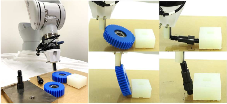
Figure 1: We consider the problem of reorienting parts for assembly using pivoting manipulation primitive. Such reorientation could possibly be required when the parts being assembled are too big to grasp in the initial pose (such as the gears) or the parts to be inserted during assembly are not in the desired pose (such as the pegs). The figure shows some instances during implementation of our controller to reorient a gear and a peg.

Contacts are central to most manipulation tasks as they provide additional dexterity to robots to interact with their environment [1]. It is desirable that a robot should be able to interact with unknown objects in unknown environments during operation and thus achieve generalizable manipulation. Robust planning for frictional interaction with objects with uncertain physical properties could be challenging as the mechanical stability of the object depends on these physical properties. Inspired by this problem, we consider the task of robust pivoting manipulation in this paper. The pivoting task considered in this paper requires that the slipping contact be maintained at the two external contact points which presents unique challenges for robust planning. We are interested in ensuring mechanical stability via friction to compensate for uncertainty in the physical properties (e.g., mass, Center of Mass (CoM) location, coefficient of friction, etc.) of the objects during manipulation. We present a formulation and an optimization technique that can solve robust manipulation trajectories for the proposed pivoting manipulation.

Robust planning (and control) for frictional interaction is challenging due to the hybrid nature of underlying frictional dynamics. Consequently, a lot of classical robust planning and control techniques are not applicable to these systems in the presence of uncertainties [2, 3, 4]. While concepts of stability margin or Lyapunov stability have been well studied in the context of nonlinear dynamical system controller design [5], such notions have not been explored in contact-rich manipulation problems. This can be mostly attributed to the fact that a controller has to reason about the mechanical stability constraints of the frictional interaction to ensure stability. Mechanical stability closely depends on the contact configuration during manipulation, and thus a planner (or controller) has to ensure that the desired contact configuration is either maintained during the task or it can maintain stability even if the contact sequence is perturbed. Analysis of such systems is difficult in the presence of friction as it leads to differential inclusion system (see [6]) . One of the key insights we present in this paper is that friction provides mechanical stability margin during a contact-rich task. We call the mechanical stability provided by friction as Frictional Stability. This frictional stability can be exploited during optimization to allow stability of manipulation in the presence of uncertainty. We show the effect of several different parameters on the stability of the manipulation using the proposed approach. In particular, we consider the effect of contact modes and point of contact between the robot & object on the stability of the manipulation. We believe that our proposed ideas could also be used for designing feedback controllers to correct contact trajectories based on estimates of contact states.

We study pivoting manipulation where the object being manipulated has to maintain slipping contact with two external surfaces (see Fig. 2). A robot can use this manipulation to reorient parts on a planar surface to allow grasping or assist in assembly by manipulating objects to a desired pose (see Fig. 1). Note that this manipulation is challenging as it requires controlled slipping (as opposed to sticking contact [7, 8, 9]), and thus it is imperative to consider robustness of the control trajectories. Ensuring robustness for slipping contact is challenging due to the equality constraints for the friction forces (compared to inequality constraints for sticking contact). To ensure mechanical stability of the two-point pivoting in the presence of uncertainty, we derive a sufficient condition for stability which allows us to compute a margin of stability. This margin is then used in a bilevel optimization routine, CIBO (Contact Implicit Bilevel Optimization), to design an optimal control trajectory while maximizing this margin. Through numerical simulations as well as physical experiments, we verify that CIBO is able to achieve more robustness compared to the basic trajectory optimization.

Contributions. This paper has the following contributions.

1. We present analysis of mechanical stability of pivoting manipulation with uncertainty in mass, CoM location, and coefficient of friction.

2. We present a robust contact-implicit bilevel optimization (CIBO) technique which can be used to optimize the mechanical stability margin to compute robust trajectories for pivoting manipulation. For objects with non-convex shapes, we present a formulation with mode-based optimization.

The proposed method is demonstrated for reorienting parts using a 6 DoF manipulator (see Fig. 1. Please see a video demonstrating hardware experiments at this link). A preliminary version of this work was initially presented at a conference [10]. However, compared to the previous work, this paper has the following major differences:

1. We present analysis of the proposed manipulation considering patch contact, and stochastic friction coefficients at the different points of contact.

2. We present a mode-based optimization formulation which can be used for computing robust trajectories for objects with non-convex geometry.

In Section II, we present work which is relevant to our proposed work. In Section III, we present the mechanics of pivoting manipulation. Section IV presents an analysis of frictional stability margin considering different sources of uncertainty. In Section V, we present the proposed contact-implicit bilevel optimization (CIBO) for robust pivoting manipulation. Section VI presents numerical results of trajectory optimization as well as experimental evaluation using a manipulator arm and several different objects. Finally, the paper is concluded in Section VII with some topics for future research.

II Related Work

Contact modeling has been extensively studied in mechanics as well as robotics literature [11, 12, 13, 14, 15, 16]. One of the most common contact models is based on the linear complementarity problem (LCP). LCP-based contacts models have been extensively used for performing trajectory optimization in manipulation [17, 18] as well as locomotion [19, 20]. More recently, there has also been some work for designing robust manipulation techniques for contact-rich systems using stochastic optimization [4, 2, 3, 21]. These problems consider stochastic complementarity systems and consider robust optimization for the underlying stochastic system. However, these problems consider a dynamical model and do not explicitly consider the mechanical stability during planning. Our work is motivated by the concepts of stability under multiple contacts in legged locomotion. Static stability with multiple contacts has been widely studied in legged locomotion [22, 23, 24, 25, 26]. These works consider the problem of mechanical stability of the legged robot under multiple contacts by considering the stability polygon defined by the frictional contacts. The planning framework for optimizing contact wrench cone margin during locomotion is able to achieve robust locomotion results [27, 25, 28]. Similar to the concept of these works, we present the idea of frictional stability which defines the extent to which multiple points of contact can compensate for unknown forces and moments in the presence of uncertainty in the mass, CoM location and frictional parameters. This idea exploits contact forces to ensure stability of the object during the two-point pivoting. Our work is also related to manipulation by shared grasping [29] which discusses mechanics of shared grasping and shows impressive demonstrations. In contrast to the work presented in [29], we present a robust contact-implicit bilevel optimization (CIBO) framework that can be used to find feasible solutions in the presence of uncertainty during the pivoting manipulation and avoids consideration of different modes during planning.

In [8], authors consider stabilization of a table-top manipulation task during online control. They consider a decomposition of the control task in object state control and contact state control. The contact state was detected using vision-based tactile sensors [30, 31]. As the task mostly required sticking contact for stability, the tactile feedback was designed to make corrections to push the system away from the boundary of friction cone at the different contact locations. However, the authors did not consider the problem of designing trajectories which can provide robustness to uncertainty. Furthermore, the authors only considered controlled sticking in [8] which is, in general, easier than controlled slipping. Other previous works that study stable pivoting also consider sticking contact during pivoting using multiple points of contact [7]. The problem in [7] is inherently stable as the object is always in stable grasp. Furthermore, the authors do not consider any uncertainty during planning. Similarly, authors in [32] present a mixed integer programming formulation to generate contact trajectory given a desired reference trajectory for the object for several manipulation primitives. In contrast, this work proposes a bilevel optimization technique which maximizes the minimum margin from instability that the object experiences during an entire trajectory. Another related work is presented in [33] where the authors study the feedback control during manipulation of a half-cylinder. The idea there is to design a reference trajectory and then use a local controller by building a funnel around the reference trajectory by linearizing the dynamics. The online control is computed by solving linear programs to locally track the reference trajectory.

From the above discussion, we can arrive at the following conclusion. In contrast to most of the related work, this proposed work presents a novel formulation for two-point pivoting which requires slipping contact formation between the object and the environment. Furthermore, in comparison to most of the work on contact implicit trajectory optimization, we present a contact implicit bilevel optimization (CIBO) for robust trajectory optimization for manipulation. Even though this method is illustrated on a particular pivoting manipulation problem in this paper, the proposed optimization algorithm could be used for other robust manipulation problems based on the mechanics of the manipulation task.

III Mechanics of Pivoting

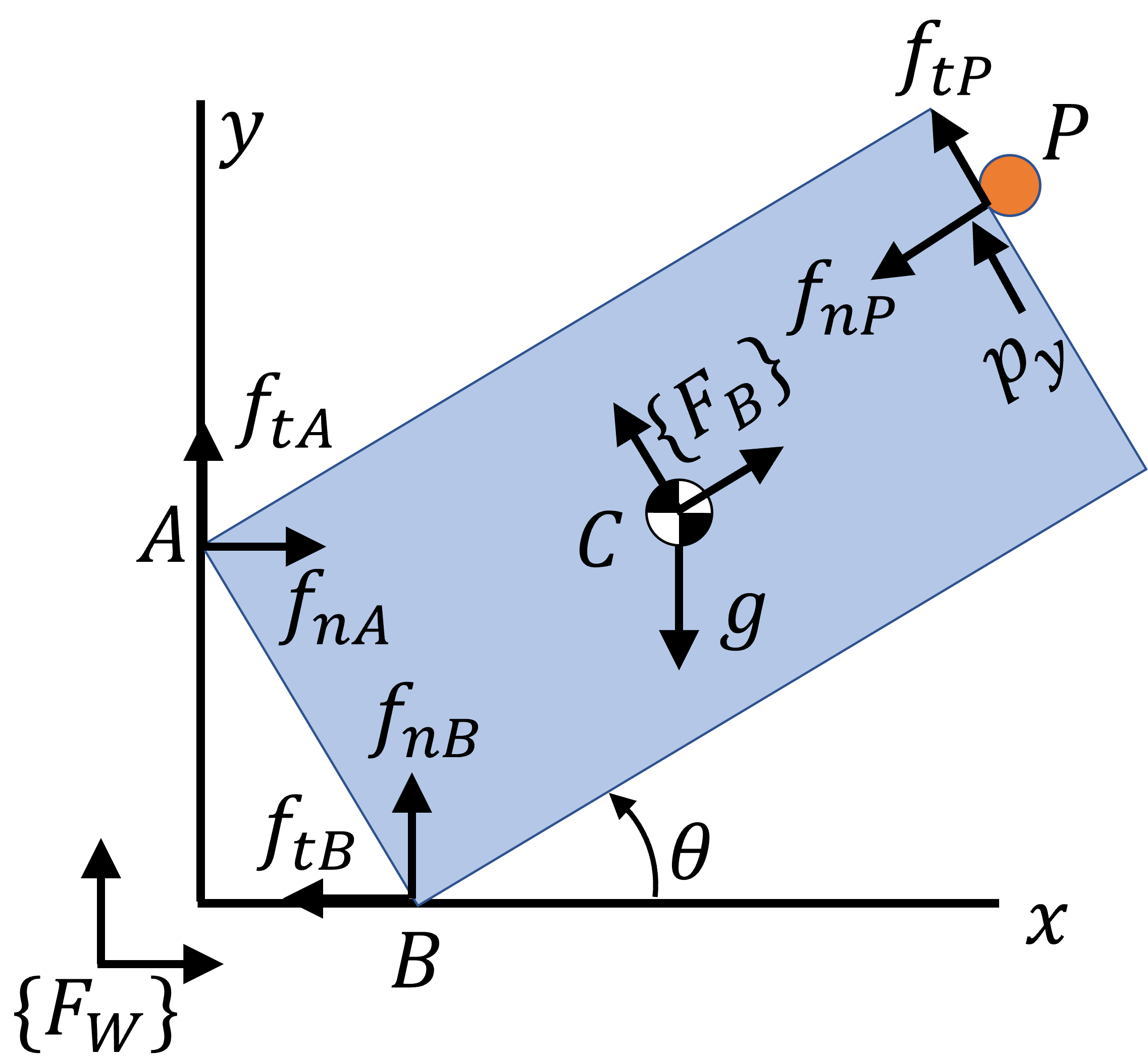
Figure 2: A schematic showing the free-body diagram of a rigid body during pivoting manipulation. Point $P$ is the contact point with a manipulator.

In this section, we explain quasi-static stability of two-point pivoting in a plane. Before explaining the details, we present our assumptions in this work. The following assumptions are used in the model for the pivoting manipulation task presented in this paper:

1. The object is rigid.

2. We consider static equilibrium of the object.

3. The external contact surfaces are perfectly flat.

4. The dimensions and pose of the object is perfectly known.

5. The object makes point contacts.

The above assumptions are common in manipulation problems.

III-A Mechanics of Pivoting with External Contacts

We consider pivoting where the object with a length of $l$ and width of $w$ maintains slipping contact with two external surfaces (see Fig. 2). A free body diagram showing the static equilibrium of the object is shown in Fig. 2. The object experiences four forces corresponding to two friction forces $f_{A},f_{B}$ from external contact points $A$ and $B$, one control input $f_{P}$ from manipulator at point $P$, and gravity, $mg$ at point $C$ where $m$ is mass of a body. We denote $f_{ni},f_{ti}$ as a normal force and friction force at point $\forall i,i=\{A,B\}$, respectively, defined in ${\{F_{W}\}}$. $f_{nP},f_{tP}$ are normal and friction force at point $P$ defined in ${\{F_{B}\}}$. Note that we define the $[f_{x},f_{y}]^{\top}=\mathbf{R}[f_{nP},f_{tP}]^{\top}$ where $\mathbf{R}$ is a rotation matrix from ${\{F_{B}\}}$ to ${\{F_{W}\}}$. We denote $x,y$ position at point in ${\{F_{W}\}}$ $\forall i,i=\{A,B,P\}$ as $i_{x},i_{y}$, respectively. We denote $y$ position of point $P$ in ${\{F_{B}\}}$ as $p_{y}\in[-\frac{w}{2},\frac{w}{2}]$. We define the angle of body with respect to $x$-axis as $\theta$. The coefficient of friction at point $\forall i,i=\{A,B,P\}$ are $\mu_{A},\mu_{B},\mu_{P}$, respectively. In the later sections, we present trajectory optimization formulation where we consider friction force variables $f_{ni},f_{ti}$, contact point variables $i_{x},i_{y}$ $\forall i,i=\{A,B,P\}$, $\theta$, and $p_{y}$ at each time-step $k$ denoted as $f_{k,ni},f_{k,ti},i_{k,x},i_{k,y},\theta_{k},p_{y,k}$. In this section, we remove $k$ to represent variables for simplicity.

The static equilibrium conditions for the object can be represented by the following equations (note we consider the moment at point $B$ by setting $B_{x}=B_{y}=0$):

$$f_{nA}+f_{tB}+f_{xP}=0,$$ (1a)

$$f_{tA}+f_{nB}+mg+f_{yP}=0,$$ (1b)

$$A_{x}f_{tA}-A_{y}f_{nA}+C_{x}mg+P_{x}f_{y}-P_{y}f_{x}=0$$ (1c)

We consider Coulomb friction law which results in friction cone constraints as follows:

$$|f_{tA}|\leq\mu_{A}f_{nA},|f_{tB}|\leq\mu_{B}f_{nB},\quad f_{nA},f_{nB}\geq 0$$ (2)

To describe sticking-slipping complementarity constraints, we have the following complementarity constraints at point $i=\{A,B\}$:

$$0\leq\dot{p}_{i+}\perp\mu_{i}f_{ni}-f_{ti}\geq 0$$ (3a)

$$0\leq\dot{p}_{i-}\perp\mu_{i}f_{ni}+f_{ti}\geq 0$$ (3b)

where the slipping velocity at point $i$ follows $\dot{p}_{i}=\dot{p}_{i+}-\dot{p}_{i-}$. $\dot{p}_{i+},\dot{p}_{i-}$ represent the slipping velocity along positive and negative directions for each axis, respectively. The notation $0\leq a\perp b\geq 0$ means the complementarity constraints $a\geq 0,b\geq 0,ab=0$. Since we consider slipping contact during pivoting, we have ”equality” constraints in friction cone constraints at points $A,B$:

$$f_{tA}=\mu_{A}f_{nA},f_{tB}=-\mu_{B}f_{nB}$$ (4)

To realize stable pivoting, actively controlling position of point $P$ is important. Thus, we consider the following complementarity constraints that represent the relation between the slipping velocity $\dot{p}_{y}$ at point $P$ and friction cone constraint at point $P$:

$$0\leq\dot{p}_{y+}\perp\mu_{p}f_{nP}-f_{tP}\geq 0$$ (5a)

$$0\leq\dot{p}_{y-}\perp\mu_{p}f_{nP}+f_{tP}\geq 0$$ (5b)

where $\dot{p}_{y}=\dot{p}_{y+}-\dot{p}_{y-}$.

IV Robust Pivoting Formulation

In this section, we present a generic formulation for robust pivoting manipulation. In particular, we use the static equilibrium conditions (1) in the presence of disturbances to formulate the robust planning problem. In particular, using sufficiency for stability of the object during manipulation we can estimate the bound of disturbance that can be tolerated during manipulation. Since this bound would depend on the pose of the object, we reason about the margin throughout the manipulation trajectory during the optimization problem formulation. We present the general idea in the following paragraph.

In the most general case, we assume that there is an external force $F_{ext}$ and moment $M_{ext}$ acting on the object during manipulation. Let us assume that the $x$ and $y$ component of the external force is represented as $F_{ext,x}$ and $F_{ext,y}$ respectively. Then the static equilibrium conditions (1) can be rewritten as follows:

$$f_{nA}+f_{tB}+f_{xP}+F_{ext,x}=0,$$ (6a)

$$f_{tA}+f_{nB}+mg+f_{yP}+F_{ext,y}=0,$$ (6b)

$$A_{x}f_{tA}-A_{y}f_{nA}+C_{x}mg+P_{x}f_{y}-P_{y}f_{x}+M_{ext}=0$$ (6c)

Note that $F_{ext}$ and $M_{ext}$ may not be independent of each other. They are related via the the point of application of force $F_{ext}$ in the static equilibrium conditions (6). These equations may not be satisfied for all possible values of $F_{ext}$ and $M_{ext}$. Since the contact forces can be readjusted in (6), the static equilibrium can be satisfied for a certain range of $F_{ext}$ and $M_{ext}$. A generic analysis for estimating this margin or bound for which these disturbances can be compensated by contact forces is a bit involved as such a bound is dependent on the point and angle of application of the external force $F_{ext}$. In the following sections, we present some specific cases which can be analyzed by making some simplifying assumptions on these disturbances.

IV-A Frictional Stability Margin

The robust quasi-static equilibrium conditions shown in (6) can be used to explain the concept of stability margin. The stability margin is given by the magnitude of the external force $F_{ext}$ and moment $M_{ext}$ which can be satisfied in (6) in any stable configuration of the object. This margin would depend on the contact force between the object and the environment as well as the control force used by the manipulator during the task. This provides the intuition that one can design a control trajectory such that the stability margin can be maximized.

We briefly provide some physical intuition about frictional stability for a few specific cases. First suppose that uncertainty exists in mass of a body. In the case when the actual mass is lower than estimated, the friction force at point $A$ would increase while the friction force at point $B$ would decrease, compared to the nominal case. In contrast, suppose if the actual mass of the body is heavier than that of what we estimate, then the body can tumble along point $B$ in the clockwise direction. In this case, we can imagine that the friction force at point $A$ would decrease while the friction force at point $B$ would increase. However, as long as the friction forces are non-zero, the object can stay in contact with the external environment. Similar arguments could be made for uncertainty in CoM location. The key point to note that the friction forces can re-distribute at the two contact locations and thus provide a margin of stability to compensate for uncertain gravitational forces and moments. We call this margin as frictional stability.

In the following sections, we present the mathematical formulation of frictional stability for cases when the mass, CoM location or friction coefficients are not known perfectly.

IV-B Stability Margin for Uncertain Mass

For simplicity, we denote $\epsilon$ as uncertain weight with respect to the estimated weight. Also, to emphasize that we consider the system under uncertainty, we put superscript $\epsilon$ for each friction force variable. Thus, the static equilibrium conditions in (1) can be rewritten as:

$$f_{nA}^{\epsilon}+f_{tB}^{\epsilon}+f_{xP}=0,$$ (7a)

$$f_{tA}^{\epsilon}+f_{nB}^{\epsilon}+(mg+\epsilon)+f_{yP}=0,$$ (7b)

$$A_{x}f_{tA}^{\epsilon}-A_{y}f_{nA}^{\epsilon}+C_{x}(mg+\epsilon)+P_{x}f_{y}-P_{y}f_{x}=0$$ (7c)

Then, using (4) and (7c), we obtain:

$$f_{nA}^{\epsilon}=\frac{-{C_{x}}\left(mg+\epsilon\right)-{P_{x}}f_{y}+{P_{y}}f_{x}}{\mu_{A}{A_{x}}-{A_{y}}}$$ (8)

To ensure that the body maintains contact with the external surfaces, we would like to enforce that the body experience non-zero normal forces at the both contacts. To realize this, we have $f_{nA}^{\epsilon}\geq 0,f_{nB}^{\epsilon}\geq 0$ as conditions that the system needs to satisfy. Consequently, by simplifying (8), we get the following:

$$\epsilon\geq\frac{P_{y}f_{x}-P_{x}f_{y}-C_{x}mg}{C_{x}},\text{ if }C_{x}>0,$$ (9a)

$$\epsilon\leq\frac{P_{y}f_{x}-P_{x}f_{y}-C_{x}mg}{C_{x}},\text{ if }C_{x}<0$$ (9b)

Note that the upper-bound of $\epsilon$ means that the friction forces can exist even when we make the mass of the body lighter up to $\frac{\epsilon}{g}$. The lower-bound of $\epsilon$ means that the friction forces can exist even when we make the mass of the body heavier up to $\frac{\epsilon}{g}$. (9) provides some useful insights. (9) gives either upper- or lower-bound of $\epsilon$ for $f_{nA}^{\epsilon}$ according to the sign of $C_{x}$ (the moment arm of gravity). This is because the uncertain mass would generate an additional moment along with point $B$ in the clock-wise direction if $C_{x}>0$ and in the counter clock-wise direction if $C_{x}<0$. If $C_{x}=0$, we have unbounded range for $\epsilon$, meaning that the body would not lose contact at point $A$ no matter how much uncertainty exists in the mass.

(9) can be reformulated as an inequality constraint:

$$C_{x}(\epsilon-\epsilon_{A})\geq 0$$ (10)

where $\epsilon_{A}=\frac{P_{y}f_{x}-P_{x}f_{y}-C_{x}mg}{C_{x}}$.

We can derive condition for $\epsilon$ based on $f_{nB}^{\epsilon}\geq 0$ from (4), (7a), and (7b):

$$\epsilon\leq\mu_{A}f_{x}-f_{y}-mg$$ (11)

We only have upper-bound on $\epsilon$ based on $f_{nB}^{\epsilon}\geq 0$, meaning that the contact at point $B$ cannot be guaranteed if the actual mass is lighter than $\mu_{A}f_{x}-f_{y}-mg$.

IV-C Stability Margin for Uncertain CoM Location

We denote $dx,dy$ as residual CoM locations with respect to the estimated CoM location in ${\{F_{B}\}}$ coordinate, respectively. Thus, the residual CoM location in $x_{W},y_{W}$, $dx_{W},dy_{W}$, are represented by $dx_{W}=d\cos({\theta+\theta_{d}}),dy_{W}=d\sin({\theta+\theta_{d}})$, where $d=\sqrt{dx^{2}+dy^{2}}$, $\theta_{d}=\arctan{\frac{dy}{dx}}$. For notation simplicity, we use $r$ to represent $dx_{W}$. In this paper, we put superscript $r$ for each friction force variables. Then, the static equilibrium conditions in (1) can be rewritten as follows:

$$f_{nA}^{r}+f_{tB}^{r}+f_{xP}=0,$$ (12a)

$$f_{tA}^{r}+f_{nB}^{r}+mg+f_{yP}=0,$$ (12b)

$$A_{x}f_{tA}^{r}-A_{y}f_{nA}^{r}+(C_{x}+r)mg+P_{x}f_{y}=P_{y}f_{x}$$ (12c)

Then, using (4) in (12), we obtain:

$$r\leq\frac{P_{y}f_{x}-P_{x}f_{y}}{mg}-C_{x},$$ (13a)

$$r\geq-C_{x}-\frac{\frac{\mu_{A}A_{x}-A_{y}}{1+\mu_{A}}(-f_{x}-f_{y}-mg)-P_{y}f_{x}+P_{x}f_{y}}{mg}$$ (13b)

where (13a), (13b) are obtained based on $f_{nA}^{r}\geq 0,f_{nB}^{r}\geq 0$, respectively. (13) means that the object would lose contact at $A$ if the actual CoM location is more to the right than our expected CoM location while the object would lose the contact at $B$ if the actual CoM location is more to the left.

IV-D Stability Margin for Stochastic Friction

In this section, we present modeling and analysis of pivoting manipulation in the presence of stochastic friction coefficients. In particular, we consider stochastic friction at the two different contact points $A$ and $B$. We do not consider stochastic friction at the contact point between the robot and the manipulator since that leads to stochastic complementarity constraints (please see [21, 4] for detailed analysis on stochastic complementarity constraints). We make the assumption that the friction coefficients at $A$ and $B$ are partially known. In particular, we assume that the friction coefficients for contact at $A$ could be represented as $\mu_{A}=\hat{\mu}_{A}+\epsilon_{\mu_{A}}$ where $\epsilon_{\mu_{A}}$ is the uncertain stochastic variable. Similarly, the friction coefficient at $B$ could be represented as $\mu_{B}=\hat{\mu}_{B}+\epsilon_{\mu_{B}}$ where $\epsilon_{\mu_{B}}$ is the uncertain stochastic variable. Note that the we do not need to need to know any information regarding the distribution of the unknown part. We can rewrite (6) for this case as follows. We put superscript $\mu$ for each friction variables:

$$f_{nA}^{\mu}+\hat{f}_{tB}^{\mu}+f_{xP}+\epsilon_{B}=0,$$ (14a)

$$\hat{f}_{tA}^{\mu}+f_{nB}^{\mu}+mg+f_{yP}+\epsilon_{A}=0,$$ (14b)

$$A_{x}\hat{f}_{tA}^{\mu}+A_{x}\epsilon_{A}-A_{y}f_{nA}^{\mu}+C_{x}mg+P_{x}f_{y}=P_{y}f_{x}$$ (14c)

where, $f_{tA}^{\mu}=\hat{f}_{tA}^{\mu}+f_{nA}^{\mu}\epsilon_{\mu_{A}}$ and $f_{tB}^{\mu}=\hat{f}_{tB}^{\mu}+f_{nB}^{\mu}\epsilon_{\mu_{B}}$. The above equations are obtained by representing $f_{nA}\epsilon_{\mu_{A}}$ as $\epsilon_{A}$ for contact at $A$ and similarly, $\epsilon_{B}$ for the contact at $B$. Thus, $\epsilon_{A}$ and $\epsilon_{B}$ are the uncertain contact forces for the contacts at $A$ and $B$. The robust formulation that we consider in this paper considers the worst-case effect of these uncertainties on the stability of the object during manipulation. Thus, we try to maximize the bound of these variables $\epsilon_{A}$ and $\epsilon_{B}$ using our proposed bilevel optimization. It is noted that $\epsilon_{A}$ and $\epsilon_{B}$ are the stability margin for this particular case of stochastic friction.

To ensure that the body maintains contact, we impose $f_{nA}^{\mu}\geq 0,f_{nB}^{\mu}\geq 0$, so that we get the following inequalities for $\epsilon_{A},\epsilon_{B}$:

$$-\mu_{A}f_{x}+\epsilon_{A}+mg+f_{y}\leq\mu_{A}\epsilon_{B}$$ (15a)

$$\epsilon_{B}\leq-\mu_{B}(\epsilon_{A}+mg+f_{y})-f_{x}$$ (15b)

To ensure slipping contact even in the presence of uncertainties, we need to satisfy friction cone constraints specified earlier in (2), (4). Using these constraints, we can find the upper and lower bound for the variables $\epsilon_{A}$ and $\epsilon_{B}$:

$$(\hat{\mu}_{A}+\epsilon_{\mu_{A}})f_{nA}^{\mu}=\hat{f}_{tA}^{\mu}+\epsilon_{\mu_{A}}f_{nA}^{\mu}$$ (16a)

$$(\hat{\mu}_{B}+\epsilon_{\mu_{B}})f_{nB}^{\mu}=-\hat{f}_{tB}^{\mu}-\epsilon_{\mu_{B}}f_{nB}^{\mu}$$ (16b)

To get a lower bound for the variables $\epsilon_{A}$ and $\epsilon_{B}$, we make a assumption regarding the uncertainty for the friction coefficients at $A$ and $B$. We assume that the unknown part is bounded above by the known part, i.e., $\epsilon_{\mu_{i}}\leq\hat{\mu}_{i}$ for $i=A,B$. Note that this is not a restrictive assumption. What this implies is that the above parameter has bounded uncertainty. For simplicity, we assume that uncertainty is bounded by the known part of the parameter. For example, if the friction coefficient is modeled as a stochastic random variable, then we assume that we know the mean of the friction parameter and the standard deviation is bounded by some multiple of mean (note that this bound is just for simplification and one can assume any practical bound for uncertainty). Consequently, we can derive the following relations:

$$-\hat{\mu}_{A}f_{nA}^{\mu}\leq\epsilon_{A}\leq\hat{\mu}_{A}f_{nA}^{\mu}$$ (17a)

$$-\hat{\mu}_{B}f_{nB}^{\mu}\leq\epsilon_{B}\leq\hat{\mu}_{B}f_{nB}^{\mu}$$ (17b)

Thus, we get constraints (15) and (17) for the stability margin by considering the stability and the friction cone constraints in the presence of uncertain friction coefficients. These constraints are used to estimate the stability margin during the proposed bilevel optimization.

IV-E Pivoting with Patch Contact between the object and the manipulator

In the previous sections, we considered point contact between the manipulator and the object. This could be potentially restrictive. Moreover, this may not be a realistic assumption when a robot is interacting with objects. In this section, we present a slightly modified formulation by considering patch contact between the object and the manipulator. We would like to analyze and understand how patch contact would compare against a point contact model for stability during pivoting manipulation. Fig. 3 shows the simplest patch contact model during the pivoting task we consider in this paper. Using this model, we can write the following quasi-static equilibrium conditions:

$$f_{nA}+f_{tB}+2f_{xP}=0,$$ (18a)

$$f_{tA}+f_{nB}+mg+2f_{yP}=0,$$ (18b)

$$A_{x}f_{tA}-A_{y}f_{nA}+C_{x}mg+\sum_{i=1}^{2}\left(P_{ix}f_{y}-P_{iy}f_{x}\right)=0$$ (18c)

where $P_{ix},P_{iy}$ represent $x$ and $y$ coordinate of $P_{1}$ and $P_{2}$ with respect to $B$, respectively. $l$ is the distance between point contact $P_{1}$ and $P_{2}$ and $l$ is a decision variable, meaning that location of $P_{2}$ is a decision variable and can change over time. In this work, we assume that $P_{1}$ does not move over time, which simplifies the model of patch contact.

Using the above static equilibrium conditions with $f_{nA}\geq 0,f_{nB}\geq 0$, we can solve and find the upper and the lower bound of stability margin under the various uncertainties described earlier in the previous subsections. We will present some results in the later section using this formulation and compare against the point contact formulation.

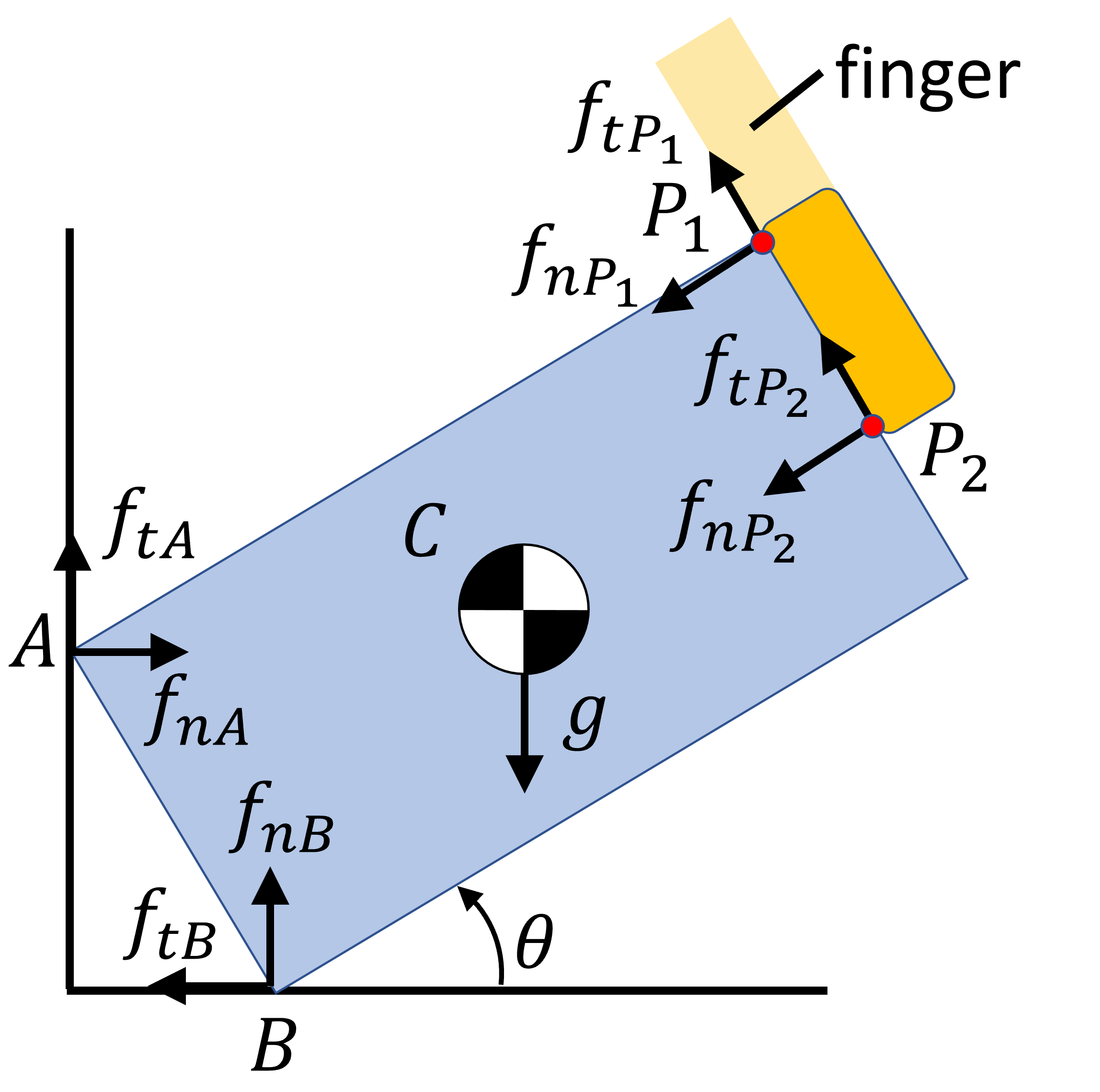
Figure 3: A schematic showing the free-body diagram of a rigid body during pivoting manipulation with patch contact. We approximate patch contact as two point contacts $P_{1}$ and $P_{2}$ with the same force distribution. We assume that $P_{1}$ always lies on the vertex of the object for this simplistic patch contact model.

V Robust Trajectory Optimization

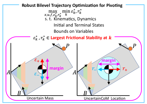
Figure 4: Conceptual schematic of our proposed frictional stability and robust trajectory optimization for pivoting. Due to slipping contact, friction forces at points $A,B$ lie on the edge of friction cone. Given the nominal trajectory of state and control inputs, friction forces can account for uncertain physical parameters to satisfy static equilibrium. We define the range of disturbances that can be compensated by contacts as frictional stability. The above figure shows the case of uncertain mass and CoM location.

Using the notion of frictional stability introduced in the previous section, we describe our proposed contact implicit bilevel optimization (CIBO) method for robust optimization of manipulation trajectories. The proposed method explicitly considers frictional stability under uncertain physical parameters. It is noted that the proposed method considers robustness under slipping contact which results in equality for friction cone constraints (see Fig. 4). After describing the formulation for convex objects, we also describe how to extend the proposed CIBO to consider objects with non-convex geometry. Our proposed method is also presented as a schematic in Fig. 4. As shown in Fig. 4, the proposed CIBO considers frictional stability margin along the entire trajectory for manipulation and then maximizes the minimum margin in the proposed framework. This is also explained in Fig. 5, where we show that we estimate the bound of stability margin in the lower level optimization and maximize the minimum margin in the upper level optimization. Before introducing our proposed bilevel optimization, we present a baseline contact-implicit TO which can be formulated as an MPCC.

V-A Contact-Implicit Trajectory Optimization for Pivoting

The purpose of our optimal control is to regulate the contact state and object state simultaneously given by:

$$\min_{x,u,f}\sum_{k=1}^{N}({x}_{k}-x_{g})^{\top}Q({x}_{k}-x_{g})+\sum_{k=0}^{N-1}u_{k}^{\top}Ru_{k}$$ (19a)

$$\text{s. t. }i_{k,x},i_{k,y}\in FK(\theta_{k},p_{k,y}),(\ref{force_eq}),(\ref{slipping_friction_cone}),(\ref{slippingP}),$$ (19b)

$$x_{0}=x_{s},x_{N}=x_{g},x_{k}\in\mathcal{X},u_{k}\in\mathcal{U},0\leq f_{k,ni}\leq f_{u}$$ (19c)

where $x_{k}=[\theta_{k},p_{k,y},\dot{\theta}_{k},\dot{p}_{k,y}]^{\top}$, $u_{k}=[f_{k,nP},f_{k,tP}]^{\top}$, $f_{k}=[f_{k,nA},f_{k,nB}]^{\top}$, $Q=Q^{\top}\geq 0,R=R^{\top}>0$. We use explicit Euler to discretize the dynamics with sample time $\Delta$. The function $FK$ represents forward kinematics to specify each contact point $i$ and CoM location. $\mathcal{X}$ and $\mathcal{U}$ are convex polytopes, consisting of a finite number of linear inequality constraints. $f_{u}$ is an upper-bound of normal force at each contact point. Note that we impose (1), (4) at each time step $k$. $x_{s},x_{g}$ are the states at $k=0,k=N$, respectively.

V-B Robust Bilevel Contact-Implicit Trajectory Optimization

Figure 5: This figure illustrates the idea of the proposed contact implicit bilevel optimization, CIBO. Given the trajectory of $x,u,f$, the stability margin over the trajectory can be computed as shown in lower-level optimization problem. Then, given the computed stability margin over the trajectory $\epsilon$, the upper-level optimization problem maximizes the worst-case stability margin over the trajectory by optimizing the trajectory of $x,u,f$. Our CIBO simultaneously optimizes the lower-level optimization problem and the upper-level optimization problem. In the right plot, red and blue arrows represent the stability margin along positive and negative directions, respectively. Our CIBO optimizes the stability margin for each direction.

In this section, we present our formulation where we incorporate frictional stability in trajectory optimization to obtain robustness. In particular, we first focus on discussing the optimization problem with uncertain mass or CoM location and we later discuss the optimization problem of uncertain coefficient of friction in Sec V-C.

An important point to note is that the optimization problem would be ill-posed if we naively add (7) and/or (12) to (19) since there is no $u$ to satisfy all uncertainty realization in equality constraints [34]. Therefore, our strategy is that we plan to find an optimal nominal trajectory that can ensure external contacts under uncertain physical parameters. In other words, we aim at maximizing the worst-case stability margin over the trajectory given the maximal frictional stability at each time-step $k$ (also shown in Fig. 4). Thus, we maximize the following objective function:

$$\min_{k}\epsilon_{k,+}^{*}-\max_{k}-\epsilon_{k,-}^{*}$$ (20)

where $\epsilon_{k,+}^{*},\epsilon_{k,-}^{*}$ are non-negative variables. Note that $\epsilon_{k,+}^{*},\epsilon_{k,-}^{*}$ are the largest uncertainty in the positive and negative direction, respectively, at instant $k$ given $x,u,f$, which results in non-zero contact forces (i.e., stability margin, see also Fig. 4). (20) calculates the smallest stability margin over time-horizons by subtracting the stability margin along the positive direction from that along the negative direction. Hence, we formulate a bilevel optimization problem which consists of two lower-level optimization problems as follows (see also Fig. 5):

$$\max_{x,u,f,\epsilon_{+}^{*},\epsilon_{-}^{*}}(\min_{k}\epsilon_{k,+}^{*}-\max_{k}-\epsilon_{k,-}^{*})\$$ (21a)

$$\text{s. t. }\quad\text{(\ref{const2}), (\ref{bounds_variables})},$$ (21b)

$$\epsilon_{k,+}^{*}\in\operatorname*{arg\,max}_{\epsilon_{k,+}}\{\epsilon_{k,+}:A_{k}\epsilon_{k,+}\leq b_{k},\epsilon_{k,+}\geq 0\},$$ (21c)

$$\epsilon_{k,-}^{*}\in\operatorname*{arg\,max}_{\epsilon_{k,-}}\{\epsilon_{k,-}:-A_{k}\epsilon_{k,-}\leq b_{k},\epsilon_{k,-}\geq 0\}$$ (21d)

where $A_{k}\in\mathbb{R}^{2\times 1},b_{k}\in\mathbb{R}^{2\times 1}$ represent inequality constraints in (10), (11). $A_{k}\epsilon_{k,+}\leq b_{k},\epsilon_{k,+}\geq 0,$ and $-A_{k}\epsilon_{k,-}\leq b_{k},\epsilon_{k,-}\geq 0$ represent the lower-level constraints for each lower-level optimization problem while (19b), (19c) represent the upper-level constraints. $\epsilon_{+},\epsilon_{-}$ are the lower-level objective functions while $\min_{k}\epsilon_{k,+}^{*}-\max_{k}-\epsilon_{k,-}^{*}$ is the upper-level objective function. $\epsilon_{k,+},\epsilon_{k,-}$ are the lower-level decision variables of each lower-level optimization problem while $x,u,f,\epsilon_{+}^{*},\epsilon_{-}^{*}$ are the upper-level decision variables.

(21) considers the largest one-side frictional stability margin along positive and negative direction at $k$. Therefore, by solving these two lower-level optimization problems, we are able to obtain the maximum frictional stability margin along positive and negative direction. The advantage of (21) is that since the lower-level optimization problem are formulated as two linear programming problems, we can efficiently solve the entire bilevel optimization problem using the Karush-Kuhn-Tucker (KKT) condition as follows:

$$w_{k,+,j},w_{k,-,j}\geq 0,C_{k}\epsilon_{k,+}\leq d_{k},E_{k}\epsilon_{k,-}\leq d_{k},$$ (22a)

$$w_{k,+,j}(C_{k}\epsilon_{k,+}-d_{k})_{j}=0,$$ (22b)

$$w_{k,-,j}(E_{k}\epsilon_{k,-}-d_{k})_{j}=0,$$ (22c)

$$\nabla(-\epsilon_{k,+})+\sum_{j=1}^{3}w_{k,+,j}\nabla(C_{k}\epsilon_{k,+}-d_{k})_{j}=0,$$ (22d)

$$\nabla(-\epsilon_{k,-})+\sum_{j=1}^{3}w_{k,-,j}\nabla(E_{k}\epsilon_{k,-}-d_{k})_{j}=0$$ (22e)

where $C_{k}=[A_{k}^{\top},-1]^{\top}\in\mathbb{R}^{3\times 1},d_{k}=[b_{k}^{\top},0]^{\top}\in\mathbb{R}^{3\times 1},E_{k}=[-A_{k}^{\top},-1]^{\top}\in\mathbb{R}^{3\times 1}$. $w_{k,+,j}$ is Lagrange multiplier associated with $(C_{k}\epsilon_{k,+}\leq d_{k})_{j}$, where $(C_{k}\epsilon_{k,+}\leq d_{k})_{j}$ represents the $j$-th inequality constraints in $C_{k}\epsilon_{k,+}\leq d_{k}$. $w_{k,-,j}$ is Lagrange multiplier associated with $(E_{k}\epsilon_{k,-}\leq d_{k})_{j}$. Using the KKT condition and epigraph trick, we eventually obtain a single-level large-scale nonlinear programming problem with complementarity constraints:

$$\max_{x,u,f,\epsilon_{+}^{*},\epsilon_{-}^{*}}(t_{+}+\alpha t_{-})\$$ (23a)

$$\text{s. t. }\quad\text{(\ref{const2}), (\ref{bounds_variables}), (\ref{kkt_equations})},$$ (23b)

$$t_{+}\leq\epsilon_{k,+},t_{-}\leq\epsilon_{k,-},\forall k$$ (23c)

where $\alpha$ is a weighting scalar. Note that we derive (23) for the case with a uncertain mass parameter but this formulation can be easily converted to the case where uncertainty exists in CoM location by replacing $A_{k},b_{k}$ in (21) with (13). Therefore, by solving tractable (23), we can efficiently generate robust trajectories that are robust against uncertain mass and CoM location parameters.

Remark 1: If we consider the case where uncertainty exists in both mass and CoM location simultaneously, we would have a nonlinear coupling term $(C_{x}+r)(mg+\epsilon)$ in static equilibrium of moment. This makes the lower-level optimization non-convex optimization, making it extremely challenging to solve during bilevel optimization.

V-C Robust Bilevel Contact-Implicit Trajectory Optimization under Frictional Uncertainty

We consider the case where the system has uncertainty in the friction coefficients at $A$ and $B$ as discussed in Sec IV-D. In order to design a robust open-loop controller for the system, we can use the similar formulation presented in Sec V-B. The proposed formulation aims at maximizing the stability margin from stochastic friction. In particular, to avoid non-convex optimization as the lower-level optimization problem, we consider the stability margin along positive and negative direction for both $\epsilon_{A}$ and $\epsilon_{B}$, as we discuss in Sec V-B. By borrowing the optimization problem (21), the proposed formulation can be seen as follows. For simplicity, we abbreviate subscript $k$.

$$\max_{x,u,f,\epsilon_{A,+}^{*},\epsilon_{A,-}^{*},\epsilon_{B,+}^{*},\epsilon_{B,-}^{*}}\sum_{c\in\mathcal{C}}(\min_{k}\epsilon_{c,+}^{*}-\max_{k}-\epsilon_{c,-}^{*})$$ (24a)

$$\text{s. t. }\quad\text{(\ref{const2}), (\ref{bounds_variables})},$$ (24b)

$$\epsilon_{A}^{*}\in[-\epsilon_{A,-}^{*},\epsilon_{A,+}^{*}],\epsilon_{B}^{*}\in[-\epsilon_{B,-}^{*},\epsilon_{B,+}^{*}],$$ (24c)

$$\epsilon_{A,+}^{*}\in\operatorname*{arg\,max}_{\epsilon_{A,+}}\{\epsilon_{A,+}:g(x,u,f,\epsilon_{A,+},\epsilon_{B}^{*})\leq 0,$$

$$\epsilon_{A,+}\geq 0\},$$ (24d)

$$\epsilon_{A,-}^{*}\in\operatorname*{arg\,max}_{\epsilon_{A,-}}\{\epsilon_{A,-}:g(x,u,f,-\epsilon_{A,-},\epsilon_{B}^{*})\leq 0,$$

$$\epsilon_{A,-}\geq 0,\},$$ (24e)

$$\epsilon_{B,+}^{*}\in\operatorname*{arg\,max}_{\epsilon_{B,+}}\{\epsilon_{B,+}:g(x,u,f,\epsilon_{B,+},\epsilon_{A}^{*})\leq 0,$$

$$\epsilon_{B,+}\geq 0,\},$$ (24f)

$$\epsilon_{B,-}^{*}\in\operatorname*{arg\,max}_{\epsilon_{B,-}}\{\epsilon_{B,-}:g(x,u,f,-\epsilon_{B,-},\epsilon_{A}^{*})\leq 0,$$

$$\epsilon_{B,-}\geq 0\},$$ (24g)

where $g$ summarizes the constraints for each lower-level optimization problem and $\mathcal{C}=\{A,B\}$. For each lower-level optimization problem, we consider that another uncertain friction is in the range of optimal stability margin. For instance, (24d) is one of the four lower-level optimization problems which aims at maximizing the stability margin under stochastic friction forces at $A$, given stochastic friction force at $B$, $\epsilon_{B}^{*}$. (24c) ensures that $\epsilon_{B}^{*}$ needs to be within the range of stability margin computed from other two lower-level optimization problems (24f) and (24g).

The resulting optimization introduces many complementarity constraints through the KKT condition because of four lower-level optimization problems, but the resulting computation is still tractable. We discuss computational results in Sec VI-G.

V-D Robust Bilevel Optimization over Mode Sequences for Non-Convex Objects

The method introduced in the previous subsections assumes convex geometry of the object being manipulated and can not be applied to objects with non-convex geometry (such as pegs as shown in Fig. 1). This is because non-convex objects could result in different contact formations between the object and the environment and it is not trivial to identify a feasible contact sequence. In [10], the proposed optimization (23) was solved sequentially for pegs with non-convex geometry. As illustrated in Fig. 6, we first solve the optimization for a particular contact set (i.e., mode 1 in Fig. 6) and then solve the optimization for another contact set (i.e., mode 2 in Fig. 6) given the solution obtained from the first optimization. While this method works, it requires extensive domain knowledge. We observed that the second stage optimization can result in infeasible solutions given the solution from the first stage optimization. Thus, we had to carefully specify the parameters of optimization and, in particular, the initial state and terminal state constraints. Such a hierarchical approach has difficulty in finding a feasible solution once the object becomes more complicated.

To overcome these issues, in general, complementarity constraints can be used to model the change of contact. However, introducing complementarity constraints inside the lower-level optimization makes the lower-level optimization non-convex optimization. Hence, the KKT condition is not a necessary and sufficient condition for optimality but rather a necessary condition. Thus, it is not guaranteed to find globally optimal safety margins over the trajectory.

In this work, we propose another approach to deal with the non-convexity of the object. Inspired by [17], we formulate the optimization that optimizes the trajectory given mode sequences instead of optimizing mode sequences. It is worth noting that our framework still optimizes the trajectory over the time duration of each mode given the sequence of the mode. Our goal is that the optimization has a larger feasible space so that less domain knowledge is required.

Figure 6: A schematic of pivoting for a non-convex shape object where contact set changes over time. During mode 1, the peg rotates with contact at $A$ and $B_{2}$. During mode 2, the peg rotates with contact at $A$ and $B_{1}$. $\gamma$ represents one of the kinematic features of peg, which is used to discuss the result in Sec 7.

Using the formulation presented in [17], we present a mode-based formulation for non-convex shaped objects. See [17] for more details regarding mode-based optimization. For simplicity of exposition, we only present the formulation considering two modes. But one can easily extend this to problems with multiple modes. For each contact mode, the system has the different constraints. For brevity, we abbreviate the subscript $k$:

$$i_{x},i_{y}\in FK_{m}(\theta_{k},p_{k,y})\forall i\in\{A,B_{m}\}$$ (25a)

$$g_{m}(f_{nA},f_{tA},f_{nB_{1}},f_{tB_{1}},f_{nP},f_{tP},p_{y})\ \text{if}\ m=1$$ (25b)

$$g_{m}(f_{nA},f_{tA},f_{nB_{2}},f_{tB_{2}},f_{nP},f_{tP},p_{y})\ \text{if}\ m=2$$ (25c)

$$f_{tA}=\mu_{A}f_{nA},f_{tB_{1}}=-\mu_{B_{1}}f_{nB_{1}},f_{tB_{2}}=-\mu_{B_{2}}f_{nB_{2}}$$ (25d)

$$(\ref{slippingP}),x_{k}\in\mathcal{X},u_{k}\in\mathcal{U},0\leq f_{k,ni}\leq f_{u}$$ (25e)

where $m\in\{1,2\}$ to represent each contact mode. $g_{m}$ represents the quasi-static model of pivoting manipulation for mode $m$. It is worth noting that since we decompose the optimization problem into the two mode optimization problem, complementarity constraints are encoded for each mode.

What the optimization problem needs to perform is that for each mode, it only considers the associated constraints and does not consider constraints associated with different contact mode. For example, during mode 1, the optimization should consider only constraints associated with mode 1 and should not consider constraints such as (25c). Another thing the optimization needs to consider is that it needs to scale $\dot{\theta},\dot{p}_{y}$ since we would like to optimize over the time duration. To achieve that, we employ the scaled time variables as discussed in [17]. As a result, we recast the quasi-static model by introducing a new state variable with a scaled time, $\tilde{x}_{k}=[\theta_{k},p_{k,y},\frac{\dot{\theta}_{k}}{T},\frac{\dot{p}_{k,y}^{\top}}{T}]$ where $T=T_{1}$ during mode 1 and $T=T_{2}$ during mode 2.

For two contact modes, we can remodel our optimization (19) as follows:

$$\min_{\tilde{x},u,f}\sum_{k=0}^{N-1}(\tilde{x}_{k}-x_{g})^{\top}Q(\tilde{x}_{k}-x_{g})+u_{k}^{\top}Ru_{k}+\sum_{l=1}^{2}T_{l}$$ (26a)

$$\text{s. t. }F_{1}(\tilde{x}_{k},u_{k},f_{k})\leq 0,\text{for}\ k\Delta\leq 1$$ (26b)

$$F_{2}(\tilde{x}_{k},u_{k},f_{k})\leq 0,\text{for}\ k\Delta>1$$ (26c)

where $\tilde{x}_{k}=[\theta_{k},p_{k,y},\frac{\dot{\theta}_{k}}{T_{1}},\frac{\dot{p}_{k,y}^{\top}}{T_{1}}]$ for $k\Delta\leq 1$ and $\tilde{x}_{k}=[\theta_{k},p_{k,y},\frac{\dot{\theta}_{k}}{T_{2}},\frac{\dot{p}_{k,y}^{\top}}{T_{2}}]$ for $k\Delta>1$. We use $F_{1}$ and $F_{2}$ to represent all constraints for each mode. Given (26), we can obtain bilevel optimization formulation for non-convex shape objects by following the logic in Sec V-B.

V-E Robust Bilevel Contact-Implicit Trajectory Optimization with Patch Contact

The formulation for robust CIBO is similar to the point contact case except that the underlying equilibrium conditions are different. The static equilibrium conditions for the patch contact case were earlier presented in (18). Using these equations and the analysis presented in Sections IV-B through IV-D, it is straightforward to compute the constraints for the corresponding robust CIBO similar to (21). More explicitly, this can be achieved by computing the appropriate constraints of the type $A_{k}\epsilon_{k,+}\leq b_{k}$ and $-A_{k}\epsilon_{k,-}\leq b_{k}$ using (18) and the frictional stability margin discussion in Sec IV-E.

VI Experimental Results

In this section, we verify the performance of our proposed approach for pivoting. Through the experiments we present in this section, we evaluate the efficacy of the proposed planner in several different settings and the computational requirement of the method. We also present results of implementation of the proposed planner on a robotic system using a 6 DoF manipulator arm and compare it against a baseline trajectory optimization method.

TABLE I: Parameters of objects. $m,l,w$ represent the mass, length, and the width of the object, respectively. For pegs, the first element in $l,w$ are $l_{1},w_{1}$ and the second element in $l,w$ are $l_{2},w_{2}$, respectively, shown in Fig. 14. For pegs, since they are made of the same material and they make contact on the same environment, we can assume $\mu_{B}=\mu_{B_{1}}=\mu_{B_{2}}$.

	$m$ [g]	$l$ [mm]	$w$ [mm]	$\mu_{A},\mu_{B},\mu_{P}$
gear 1	140	84	20	0.3, 0.3, 0.8
gear 2	100	121	9.5	0.3, 0.3, 0.8
gear 3	280	84	20	0.3, 0.3, 0.8
peg 1	45	36, 40	20, 28	0.3, 0.3, 0.8
peg 2	85	28, 40	10, 11	0.3, 0.3, 0.8
peg 3	85	28, 40	10, 27.5	0.3, 0.3, 0.8

Figure 7: Trajectory of frictional stability margin. $\epsilon_{A},\epsilon_{B}$ are bounds of $\epsilon$ from (10), (11). $r_{A},r_{B}$ are bounds of $r$ from (13). $\epsilon_{+},\epsilon_{-},r_{+},r_{i}$ are solutions obtained from CIBO. (a), (b): Trajectory of frictional stability of gear 1 based on uncertain mass obtained from baseline optimization, our CIBO, respectively. (c), (d): Trajectory of frictional stability of gear 1 based on uncertain CoM location obtained from baseline optimization, CIBO, respectively. (e): Snapshots of pivoting motion for gear 1 obtained from CIBO considering uncertain CoM location.

Figure 8: (a), (b): Trajectory of frictional stability margin of peg 1 based on uncertain mass obtained from CIBO, baseline optimization, respectively. Note that here we solve CIBO sequentially for each mode (i.e., hierarchical planning), instead of using the proposed mode-sequence-based optimization. (c): Snapshots of pivoting motion for peg 1, obtained from CIBO considering uncertain mass.

Figure 9: We show the time history of object angle, finger position, and contact forces from a manipulator during pivoting of gear 1. The top row shows the result using CIBO (23) considering CoM uncertainty and the bottom one shows the result using (19) (i.e., it does not consider robustness criteria in the formulation explicitly.). The top row results and the bottom row results are used in visualizing the stability margin in Fig. 7 (d), (c), respectively.

TABLE II: Worst-case stability margin over the control horizon obtained from optimization for gear 1. Note that the stability margin for the solution of the benchmark optimization is analytically calculated.

	$\epsilon_{+}^{*}$, $\epsilon_{-}^{*}$ [N]	$r_{+}^{*}$, $r_{-}^{*}$ [mm]
Benchmark optimization (19)	0.10, 0.66	1.5, 0.85
Ours (23) with mass uncertainty	0.34, 0.50	N/A
Ours (23) with CoM uncertainty	N/A	3.43, 2.70

TABLE III: Obtained worst stability margins over the time horizons from optimization for peg 1. Note that the stability margin for the solution of the benchmark optimization is analytically calculated.

	$\epsilon_{+}^{*}$, $\epsilon_{-}^{*}$ [N]	$r_{+}^{*}$, $r_{-}^{*}$ [mm]
Benchmark optimization (19)	0.035, 0.018	31, 0
Ours (23) with mass uncertainty	0.050, 0.021	N/A
Ours (23) with CoM uncertainty	N/A	38, 0

VI-A Experiment Setup

We implement our method in Python using IPOPT solver [35] with PyRoboCOP wrapper [17, 36]. We use HSL MA86 [37] as a linear solver for IPOPT. The optimization problem is implemented on a computer with Intel i7-12800K.

We demonstrate our algorithm on several different objects, as detailed in Table I. During optimization, we set $Q=\text{diag}(0.1,0),R=\text{diag}(0.01,0.01)$. We use $\alpha=1$ when we run (23). We set $x_{s}=[0,\frac{w}{4}]^{\top},\theta_{g}=\frac{\pi}{2}$. Note that we only enforce terminal constraints for convex shape objects. For non-convex shape objects, we do not enforce terminal constraints since the peg cannot achieve $\theta_{N}=\frac{\pi}{2}$ unless we consider another contact mode (see Fig. 6). In PyRoboCOP wrapper, we did warm-start for the state at $k=0,N$ by setting initial and terminal states as initial guesses. We did not explicitly conduct a warm-start for other decision variables and we set them to 0.

We use a Mitsubishi Electric Factory Automation (MELFA) RV-5AS-D Assista 6 DoF arm (see Fig. 1) for the experiments. The robot has a pose repeatability of $\pm 0.03$mm. The robot is equipped with Mitsubishi Electric F/T sensor 1F-FS001-W200 (see Fig. 1). To implement the computed force trajectory during manipulation, we use the default stiffness controller for the robot. By selecting an appropriate stiffness matrix [38], we design a reference trajectory that would result in the desired interaction force required for manipulation [39, 40]. Note that this trajectory is implemented in open-loop and we do not design a controller to ensure that the computed force trajectory is precisely tracked during execution.

VI-B Results of Bilevel Optimization for Uncertain Mass and CoM Parameters

Fig. 7 shows the trajectory of frictional stability margin of gear 1 obtained from the proposed robust CIBO considering uncertain mass and uncertain CoM location, and the benchmark optimization. Overall, CIBO could generate more robust trajectories. For example, at $t=0$ s, $f_{nB}$ in (a) is almost zero so that the stability margin obtained from (11) is almost zero. In contrast, CIBO could realize non-zero $f_{nB}$ as shown as a red arrow in (b). In (d), to increase the stability margin, the finger position $p_{y}$ moves on the face of gear 1 so that the controller can increase the stability margin more than the benchmark optimization. This would not happen if we do not consider complementarity constraints (5). Also, our obtained $\epsilon_{+},\epsilon_{-},r_{+},r_{-}$ follows bounds of stability margin. It means that CIBO can successfully design a controller that maximizes the worst stability margin given the best stability margin for each time-step.

Fig. 9 shows that both the benchmark and CIBO actually change the finger position $p_{y}$ by considering complementarity constraints (5). In fact, we observed that at $t=25$ s, $p_{y}$ in both results moves to the negative value to maintain the stability of the object. In practice, we are unable to find any feasible solutions with fixed $p_{y}$, instead of using (5). Thus, (5) is critically important to find a feasible solution.

Next, we discuss how much CIBO improves the worst-case stability margin. The trajectories of $f_{np}$ in Fig. 9 show that the magnitude of $f_{np}$ from CIBO increase at $t=25$ s to improve the worst-case stability margin. On the other hand, $f_{np}$ from the benchmark optimization does not increase at $t=25$ s. Hence, we verify that by increasing normal force, the robot could successfully robustify the pivoting manipulation. This result can be also understood in Fig. 7 (c) and (d) where the stability margin in (d) at $t=25$ s is larger than that in (c), as discussed above.

Table II and Table III summarize the computed stability margin from Fig. 7. In Table II, for the case where CIBO considers uncertainty of mass, we observe that the value of $\epsilon_{-}^{*}$ from CIBO is smaller than that from the benchmark optimization although the sum of the stability margin $\epsilon_{+}^{*}+\epsilon_{-}^{*}$ from CIBO is greater than that from the benchmark optimization. This result means that CIBO can actually improve the worst-case performance by sacrificing the general performance of the controller. Regarding the case where we consider the uncertain CoM location, CIBO outperforms the benchmark trajectory optimization in both $r_{+}^{*},r_{-}^{*}$. For peg 1, the bilevel optimizer without using mode sequence-based optimization (i.e., hierarchical optimization) finds trajectories that have larger stability margins for both uncertain mass and CoM location as shown in Table III. The trajectory of stability margin obtained from CIBO considering mass uncertainty is illustrated in Fig. 8. We discuss the results using CIBO with mode-sequence based optimization in Sec VI-E.

VI-C Results of Bilevel Optimization with Different Manipulator Initial State

Figure 10: Time history of frictional stability margin considering CoM location with different initial manipulator position $p_{y}(t=0)$.

TABLE IV: Computed worst-case stability margin considering uncertain CoM location with different $p_{y}$ at $t=0$ over the control horizon obtained from optimization for gear 1.

	$r_{+}^{*}$, $r_{-}^{*}$ [mm]
Ours with $p_{y}(t=0)=0$	16.47, 1.36
Ours with $p_{y}(t=0)=0.125w$	12.99, 2.98
Ours with $p_{y}(t=0)=0.25w$	10.00, 4.41
Ours with $p_{y}(t=0)=0.375w$	5.94, 5.67
Ours with $p_{y}(t=0)=0.5w$	1.94, 6.77

We believe that the efficiency of the optimization depends on the initial location of the manipulator finger. This is because the stability margin depends on the manipulation finger location, which is partially governed by its location at $t=0$. Thus we present some results by randomizing over the manipulator finger location at $t=0$. We sample initial state of finger position $p_{y}(t=0)$ from a discrete uniform distribution with the range of $p_{y}(t=0)\in[-0.5w,-0.375w,-0.25w,-0.125w,\ldots,0.5w]$. Then we run CIBO considering CoM location uncertainty.

Fig. 10 illustrates the time history of stability margin with different $p_{y}(t=0)$. CIBO is not able to find feasible solutions with $p_{y}(t=0)<0$. It makes sense since there may not be enough moment for the desired motion if $p_{y}(t=0)<0$.

Fig. 10 shows that different $p_{y}(t=0)$ leads to different stability margin over the time horizon. Table IV summarizes the worst-case stability margin over the trajectory obtained from Fig. 10. Table IV also shows that the worst-case stability margin is different with different $p_{y}(t=0)$. Finding a good $p_{y}(t=0)$ is not trivial and it requires domain knowledge. Thus, ideally, we should formulate CIBO where $p_{y}(t=0)$ is also a decision variable so that the solver can optimize the trajectory over $p_{y}(t=0)$ as well.

Since CIBO is non-convex optimization, it is still possible that a feasible solution exists for $p_{y}(t=0)<0$. However, we can at least argue that it is much more difficult to find a feasible solution with $p_{y}(t=0)<0$ than that with $p_{y}(t=0)\geq 0$.

VI-D Results of Bilevel Optimization for Uncertain Friction Parameters

Fig. 11 shows the time history of frictional stability margin of gear 1 and gear 3 using (24). CIBO could successfully design an optimal open-loop trajectory by improving the worst-case performance of stability margin. We observe that Fig. 11 (b) shows a larger stability margin compared to (a). This result makes sense since in (b), we consider gear 3 whose weight is heavier than the weight of gear 1 and thus we get stability margins which are bigger than those obtained for (a).

(a)

(b)

Figure 11: Trajectory of frictional stability margin of (a) gear 1 and (b) gear 3, based on uncertain friction obtained from CIBO (24), respectively.

VI-E Results of Bilevel Optimization over Mode Sequences for Non-Convex Objects

In this section, we present results for objects with non-convex geometry using the mode-based optimization presented in Section V-D. Fig. 12 shows the time history of states, control inputs, and frictional stability margins for pegs whose geometry are non-convex and the contact sets change over time. First of all, we can observe that CIBO in (26) could successfully optimize the stability margin over trajectory while it optimizes the time duration of each mode. We observe that $\frac{T_{1}}{T_{1}+T_{2}}$ (i.e., the ratio of mode 1 over the horizon) of peg 2 is much smaller than that of peg 3 since $\gamma$ (see Fig. 6 for the definition of $\gamma$) of peg 2 is smaller than that of peg 3 and thus, it spends less time in mode 1. Fig. 12 shows that $f_{tp}$ of peg 3 dramatically changes at $t=T_{1}$ s while that of peg 1 does not. In contrast, the shape of peg 2 has smaller $\gamma$ (i.e., less non-convex shape) and it can be regarded as a rectangle shape. Thus, the effect of contact mode is less, leading to smaller change of $f_{tp}$ at $t=T_{1}$ s.

In order to show that we can find solutions much more effortlessly using (26) compared to two-stage optimization (that was earlier used in [10]), we sample 20 different $p_{y}$ at $t=0$ s and count the number of times the benchmark two-stage optimization problem and the proposed optimization problem over the mode sequences (26) can find feasible solution. We observed that the benchmark two-stage optimization problem found feasible solutions only 2 times while the mode-based optimization using (26) was successfully able to find feasible 18 out of 20 times. Therefore, we verify that our proposed optimization problem enables to find solutions much more effortlessly. The benchmark method requires careful selection of parameters to ensure feasibility (as was explained in [10]).

Figure 12: We show the time history of object angle, finger position, contact forces from a manipulator, and frictional stability margins. The top row shows the result with peg 2 and the bottom one shows the result with peg 3. The pink and blue shade regions represent that the system follows mode 1 and mode 2, respectively.

VI-F Results of Bilevel Optimization for Patch Contact

Table VIII shows the computed stability margin considering patch contact shows the greater margins for both positive and negative directions. Hence, we verify that our optimization can still work with patch contact and design the robust controller for maximizing the worst-case stability margin. Intuitively, this result makes sense since the contact area increases and the pivoting system has a larger physically feasible space, resulting in a greater stability margin.

Fig. 13 illustrates the time history of frictional stability margin of gear 2 from CIBO with considering point contact and with considering patch contact. Both CIBO with point contact and patch contact have the smallest (i.e., worst-case) stability margin at $t=0$. However, CIBO with patch contact shows a greater margin at $t=0$, as we discuss above. In addition, over the trajectory, CIBO with patch contact shows a greater margin than that with point contact. Thus, we quantitatively verify that using patch contact is beneficial over the trajectory even though the optimization aims at maximizing the worst-case margin, not the stability margin over the trajectory. It is noted that we are not able to obtain better margins using patch contact due to the non-convexity of the underlying optimization problem.

TABLE V: Average Solving Time (AST) comparison between benchmark optimization (19) and CIBO under mass uncertainty using (23) with gear 2.

$N$	AST (s) of (19)	AST (s) of (23)
30	0.21	0.38
60	0.50	0.68
120	1.01	1.24

VI-G Computation Results

Table V compares the computation time between benchmark optimization (19) and CIBO under mass uncertainty using (23) for gear 2. Overall, (23) is not so computationally demanding compared to (19). However, as you can see in Table VI and Table VII, once the optimization problem has too many complementarity constraints because of the KKT condition, we clearly observe that the computational time increases.

Table VI and Table VII shows the computational results for CIBO considering frictional uncertainty (24) and bilevel optimization over mode sequences (26), respectively.

In general, the computational time for CIBO is larger than the benchmark optimization as CIBO has larger number of complementarity constraints. In the future, we will try to work on better warm-starting strategies so that we might be able to accelerate the optimization.

TABLE VI: NLP specification for CIBO under frictional uncertainty using (24) with gear 1.

$N$	$\#$ of Variables	$\#$ of Constraints	Average Solving Time (s)
30	2339	2280	1.9
60	4679	4560	10.6
120	9359	9130	30.9

TABLE VII: NLP specification for CIBO over mode sequences considering uncertain CoM location using (26) with peg 3.

$N$	$\#$ of Variables	$\#$ of Constraints	Average Solving Time (s)
30	1648	1590	3.68
60	3298	3180	61.6
120	6598	6360	73.0

TABLE VIII: Computed worst-case stability margin considering uncertain CoM location over the control horizon obtained from optimization for gear 2.

	$r_{+}^{*}$, $r_{-}^{*}$ [mm]
Ours with point contact	5.27, 1.31
Ours with patch contact	6.81, 8.82

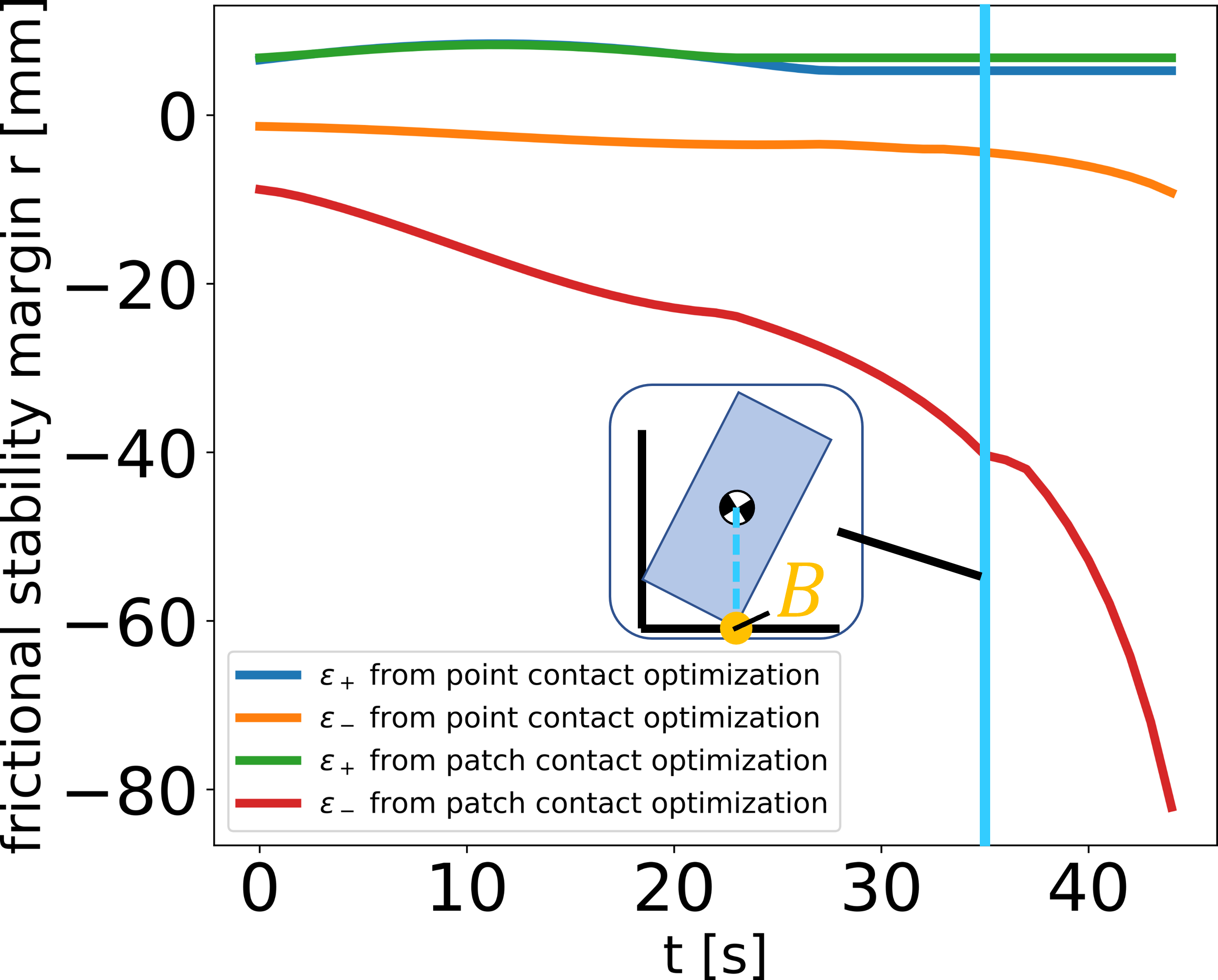
Figure 13: Trajectory of frictional stability margin of gear 2 based on uncertain CoM obtained from CIBO using point contact model and patch contact model, respectively. The vertical blue line represents the moment when the projection of CoM lies on the contact $B$.

VI-H Hardware Experiments

We implement our controller using a 6 DoF manipulator to demonstrate the efficacy of our proposed method. In particular, we perform a set of experiments to compare our method against a baseline method using gear 1. To evaluate robustness for objects with unknown mass, we solve the optimization with mass different from the true mass of the object and implement the obtained trajectory on the object. We implement trajectories obtained from the two different optimization techniques using 4 different mass values.

TABLE IX: Number of successful pivoting attempts of gear 1 over 10 trials for the two different methods. To evaluate robustness for objects with unknown mass, we solve the optimization with mass different from the known object and implement the obtained trajectory on the object with known mass. Note that the actual mass of gear 1 is 140 gm.

	CIBO	Benchmark Optimization
$m=100$ g	10 / 10	0 / 10
$m=110$ g	10 / 10	0 / 10
$m=140$ g	10 / 10	0 / 10
$m=170$ g	10 / 10	0 / 10

Table IX shows the success rate of pivoting for the hardware experiments. We observe that our proposed bilevel optimization is able to achieve 100 $\%$ success rates for all $4$ mass values while benchmark optimization cannot realize stable pivoting. Note that the benchmark trajectory optimization also generates trajectories with non-zero frictional stability margin but they failed to pivot the object. The reason would be that the system has a number of uncertainties such as incorrect coefficient of friction, sensor noise in the F/T sensor (for implementing the force controller), etc. which are not considered in the model. We believe that these uncertainties make the objects unstable leading to the failure of pivoting. In contrast, even though CIBO also does not consider these uncertainties, it generates more robust trajectories and we believe that this additional robustness could account for the unknown uncertainty in the real hardware. We also observe that the trajectories generated by benchmark optimization can successfully realize pivoting if the manipulator uses patch contact during manipulation (thus getting more stability).

We perform hardware experiments with additional objects to evaluate the generalization of the proposed planning method. All the objects used in the hardware experiments are shown in Fig. 15. A video describing the hardware experiments with all the object can be found at this link https://www.youtube.com/watch?v=ojlZDaGytSY. Fig. 14 shows the snapshots of hardware experiments for the 4 objects detailed in Table I. We observe that our bilevel optimization can successfully pivot all the objects during hardware experiments (see Fig. 14 and the videos). This shows that we can use the proposed method with objects with different size and shape.

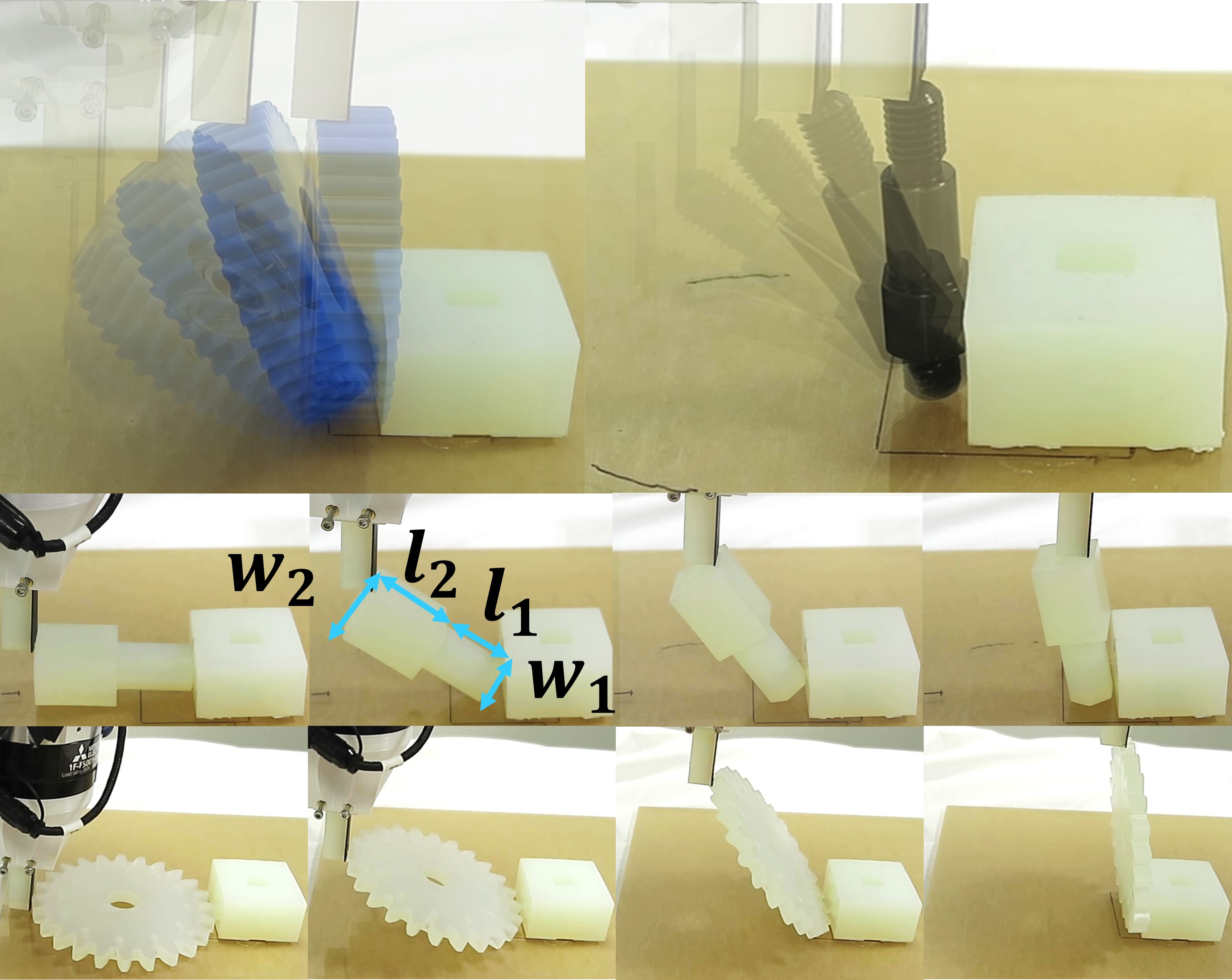
Figure 14: Snapshots of hardware experiments. We show snapshots of the white peg and gear (instead of overlaid images) for clarity.

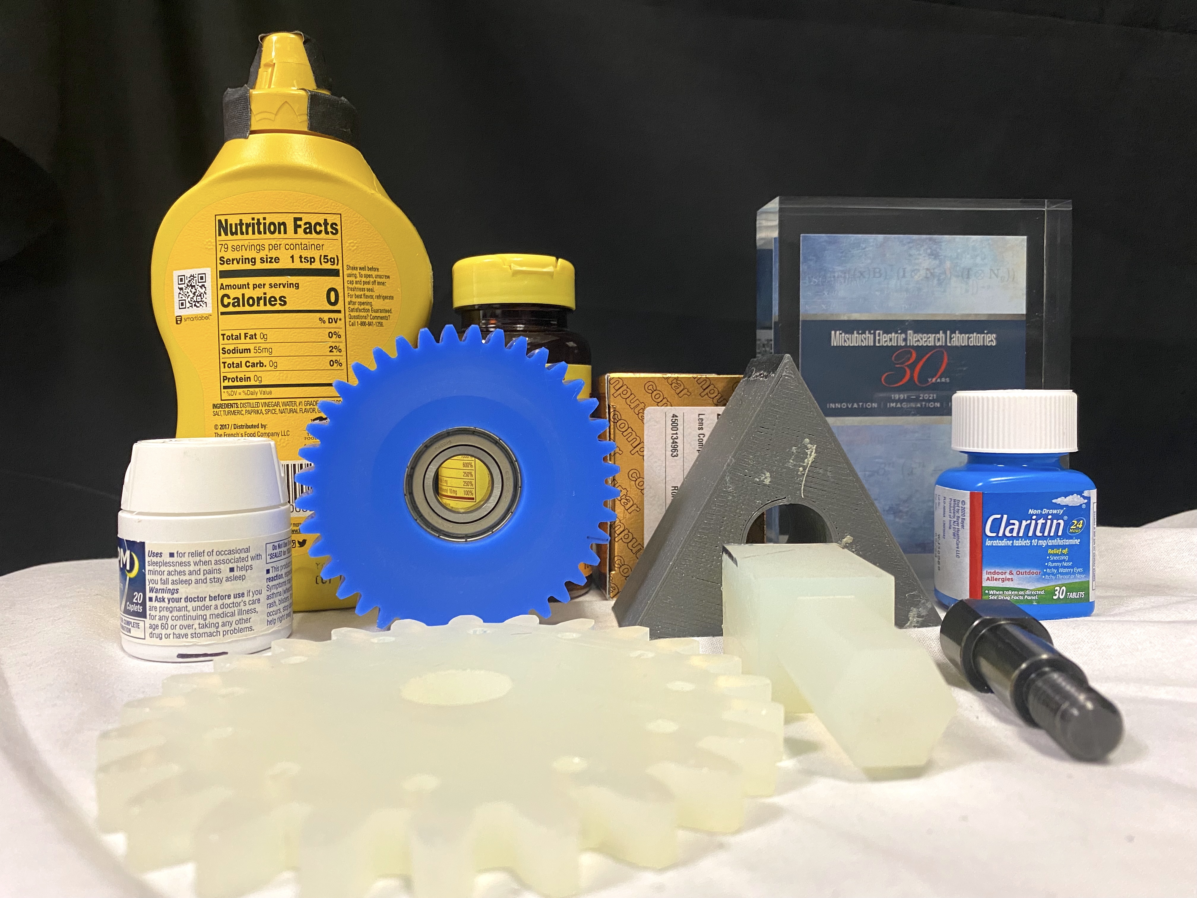
Figure 15: The different objects used in hardware evaluation of the proposed method. Please check the hardware experiments results in the video at this link https://www.youtube.com/watch?v=ojlZDaGytSY.

VII Discussion and Future Work

Generalizable manipulation through contact requires that robots be able to incorporate and account for uncertainties during planning. However, designing the robust controller for achieving such manipulation remains an open problem and remains largely unexplored. This paper presents frictional stability-aware optimization, a strategy that exploits friction for robust planning of pivoting manipulation. By considering a variety sources of uncertainty such as mass, CoM location, and friction coefficients, we discussed the stability margin for pivoting manipulation with slipping contact. We presented CIBO, which solves novel bilevel optimization for pivoting manipulation while optimizing the worst-case stability margin of pivoting manipulation for (non-convex) objects. The proposed method was evaluated in simulation using several test settings. We showed that our proposed bilevel optimization method is able to design trajectories which are robust to larger uncertainties compared to a baseline trajectory optimization method. The proposed method was also demonstrated on a physical robotic system by implementing the computed trajectories in an open-loop fashion.

Although this paper focuses on pivoting manipulation as a demonstration of our framework, our work can be generalized to other manipulation primitives such as pivoting with one-point contact, pushing, and grasping. This is because our stability margin analysis and CIBO are derived from static force and moment balance equations (1) and the corresponding friction cone constraints (2). These conditions are very common across most manipulation problems, and thus our framework can be applicable to the aforementioned manipulation primitives as long as they satisfy (1) and (2).

There are a number of limitations in this work:

Contact-Rich CIBO This work assumes that dynamics of an object with quasi-static equilibrium. For objects with non-convex geometry, CIBO is still able to design robust open-loop controller using mode-based optimization. CIBO using mode-based optimization is able to find feasible solutions if users can provide CIBO with physically feasible mode sequences. However, for objects with a very complex shape, it is quite challenging to identify mode sequences prior to optimization. As a result, CIBO might not be able to find feasible solutions. In order to avoid providing mode sequences, CIBO needs to consider mode sequences by itself. This can be realized by considering complementarity constraints or integer constraints inside the lower-level optimization problem of CIBO. However, as we explained in Sec V-D, CIBO considering these non-convex constraints inside the lower-level optimization problem is not guaranteed to find globally optimal safety margins.

Dynamic Manipulation with Uncertainty Propagation In this work, we assume quasi-static assumption for objects. The natural extension of this work is to relax this assumption and consider quasi-dynamic model during manipulation. To work on these cases, we need to explicitly consider dynamic version of the stability margin. However, this is not trivial. We need to understand how we can propagate uncertainty for contact dynamics as it is not well understood. The stability margin needs to incorporate this uncertainty propagation for such cases. See [21] for more discussion about how uncertainty propagates for contact-rich dynamical systems.

Accurate Contact Mechanics One of the contributions of this paper is that we consider patch contact. However, in reality, the robot should be able to switch contact mode from patch contact to point contact and vice versa. This enables CIBO to have a larger stability margin but, again, makes the lower-level optimization of CIBO non-convex.

Another limitation here is modeling of compliant contact. We observed that introducing compliant contact improves the stability of the object. However, modeling compliant contact is difficult. One approach to model compliant contact can be learning-based approach.

One of the assumptions of this work is that we consider pivoting in 2D. Thus, extending our work in 3D is promising, which requires the discussion of generalized friction cones [41].

Closed Loop Control The focus of this work is robust planning for pivoting in the presence of uncertainties. However, for most of practical applications we want closed-loop control of manipulation using sensory feedback. Without a closed-loop controller, even the robust trajectories need to be initialized precisely and the system can not recover from a failure. In the future, we would like to design a closed-loop controller using vision and tactile sensing for precise control of manipulation [9, 42].

References

- [1] M. T. Mason, “Toward robotic manipulation,” Annual Review of Control, Robotics, and Autonomous Systems, vol. 1, pp. 1–28, 2018.
- [2] L. Drnach and Y. Zhao, “Robust trajectory optimization over uncertain terrain with stochastic complementarity,” IEEE Robotics and Automation Letters, vol. 6, no. 2, pp. 1168–1175, 2021.
- [3] J. Z. Zhang, L. Drnach, and Y. Zhao, “Mediating between contact feasibility and robustness of trajectory optimization through chance complementarity constraints,” CoRR, vol. abs/2105.09973, 2021.
- [4] Y. Shirai, D. Jha, A. Raghunathan, and D. Romeres, “Chance constrained optimization in contact-rich systems for robust manipulation,” in 2023 American Control Conference (ACC), accepted.
- [5] M. Vidyasagar, Nonlinear systems analysis. SIAM, 2002.
- [6] A. U. Raghunathan and J. T. Linderoth, “Stability analysis of discrete-time linear complementarity systems,” arXiv preprint arXiv:2012.13287, 2020.
- [7] Y. Hou, Z. Jia, and M. T. Mason, “Fast planning for 3d any-pose-reorienting using pivoting,” in 2018 IEEE International Conference on Robotics and Automation (ICRA). IEEE, 2018, pp. 1631–1638.
- [8] F. R. Hogan, J. Ballester, S. Dong, and A. Rodriguez, “Tactile dexterity: Manipulation primitives with tactile feedback,” in 2020 IEEE international conference on robotics and automation (ICRA). IEEE, 2020, pp. 8863–8869.
- [9] Y. Shirai, D. K. Jha, A. U. Raghunathan, and D. Hong, “Tactile tool manipulation,” in 2023 International Conference on Robotics and Automation (ICRA). IEEE, accepted.
- [10] Y. Shirai, D. K. Jha, A. U. Raghunathan, and D. Romeres, “Robust pivoting: Exploiting frictional stability using bilevel optimization,” in 2022 International Conference on Robotics and Automation (ICRA), 2022, pp. 992–998.
- [11] E. Todorov, “Implicit nonlinear complementarity: A new approach to contact dynamics,” in 2010 IEEE international conference on robotics and automation. IEEE, 2010, pp. 2322–2329.
- [12] E. Drumwright and D. A. Shell, “An evaluation of methods for modeling contact in multibody simulation,” in 2011 IEEE International Conference on Robotics and Automation. IEEE, 2011, pp. 1695–1701.
- [13] C. de Farias, N. Marturi, R. Stolkin, and Y. Bekiroglu, “Simultaneous tactile exploration and grasp refinement for unknown objects,” IEEE Robotics and Automation Letters, vol. 6, no. 2, pp. 3349–3356, 2021.
- [14] Y. Shirai, X. Lin, A. Schperberg, Y. Tanaka, H. Kato, V. Vichathorn, and D. Hong, “Simultaneous contact-rich grasping and locomotion via distributed optimization enabling free-climbing for multi-limbed robots,” in 2022 IEEE/RSJ International Conference on Intelligent Robots and Systems (IROS), 2022, pp. 13 563–13 570.
- [15] Y. Zhu, Z. Pan, and K. Hauser, “Contact-implicit trajectory optimization with learned deformable contacts using bilevel optimization,” in 2021 IEEE International Conference on Robotics and Automation (ICRA), 2021, pp. 9921–9927.
- [16] S. Shield, A. M. Johnson, and A. Patel, “Contact-implicit direct collocation with a discontinuous velocity state,” IEEE Robotics and Automation Letters, vol. 7, no. 2, pp. 5779–5786, 2022.
- [17] A. U. Raghunathan, D. K. Jha, and D. Romeres, “PYROBOCOP : Python-based robotic control & optimization package for manipulation and collision avoidance,” CoRR, vol. abs/2106.03220, 2021.
- [18] S. Jin, D. Romeres, A. Ragunathan, D. K. Jha, and M. Tomizuka, “Trajectory optimization for manipulation of deformable objects: Assembly of belt drive units,” arXiv preprint arXiv:2106.00898, 2021.
- [19] M. Posa, C. Cantu, and R. Tedrake, “A direct method for trajectory optimization of rigid bodies through contact,” The International Journal of Robotics Research, vol. 33, no. 1, pp. 69–81, 2014.
- [20] A. Patel, S. L. Shield, S. Kazi, A. M. Johnson, and L. T. Biegler, “Contact-implicit trajectory optimization using orthogonal collocation,” IEEE Robotics and Automation Letters, vol. 4, no. 2, pp. 2242–2249, 2019.
- [21] Y. Shirai, D. K. Jha, and A. U. Raghunathan, “Covariance steering for uncertain contact-rich systems,” in 2023 International Conference on Robotics and Automation (ICRA). IEEE, accepted.
- [22] T. Bretl and S. Lall, “Testing static equilibrium for legged robots,” IEEE Transactions on Robotics, vol. 24, no. 4, pp. 794–807, 2008.
- [23] A. Del Prete, S. Tonneau, and N. Mansard, “Zero step capturability for legged robots in multicontact,” IEEE Transactions on Robotics, vol. 34, no. 4, pp. 1021–1034, 2018.
- [24] K. Hauser, S. Wang, and M. R. Cutkosky, “Efficient equilibrium testing under adhesion and anisotropy using empirical contact force models,” IEEE Transactions on Robotics, vol. 34, no. 5, pp. 1157–1169, 2018.
- [25] R. Orsolino, M. Focchi, C. Mastalli, H. Dai, D. G. Caldwell, and C. Semini, “Application of wrench-based feasibility analysis to the online trajectory optimization of legged robots,” IEEE Robotics and Automation Letters, vol. 3, no. 4, pp. 3363–3370, 2018.
- [26] Y. Shirai, X. Lin, Y. Tanaka, A. Mehta, and D. Hong, “Risk-aware motion planning for a limbed robot with stochastic gripping forces using nonlinear programming,” IEEE Robotics and Automation Letters, vol. 5, no. 4, pp. 4994–5001, 2020.
- [27] H. Dai and R. Tedrake, “Planning robust walking motion on uneven terrain via convex optimization,” in 2016 IEEE-RAS 16th International Conference on Humanoid Robots (Humanoids). IEEE, 2016, pp. 579–586.
- [28] H. Audren and A. Kheddar, “3-d robust stability polyhedron in multicontact,” IEEE Transactions on Robotics, vol. 34, no. 2, pp. 388–403, 2018.
- [29] Y. Hou, Z. Jia, and M. Mason, “Manipulation with shared grasping,” in Robotics: Science and Systems, 2020.
- [30] E. Donlon, S. Dong, M. Liu, J. Li, E. Adelson, and A. Rodriguez, “Gelslim: A high-resolution, compact, robust, and calibrated tactile-sensing finger,” in 2018 IEEE/RSJ International Conference on Intelligent Robots and Systems (IROS). IEEE, 2018, pp. 1927–1934.
- [31] W. Li, A. Alomainy, I. Vitanov, Y. Noh, P. Qi, and K. Althoefer, “F-touch sensor: Concurrent geometry perception and multi-axis force measurement,” IEEE Sensors Journal, vol. 21, no. 4, pp. 4300–4309, 2020.
- [32] B. Aceituno-Cabezas and A. Rodriguez, “A global quasi-dynamic model for contact-trajectory optimization,” in Robotics: Science and Systems (RSS), 2020.
- [33] W. Han and R. Tedrake, “Local trajectory stabilization for dexterous manipulation via piecewise affine approximations,” in 2020 IEEE International Conference on Robotics and Automation (ICRA). IEEE, 2020, pp. 8884–8891.
- [34] “Equalities with uncertainty,” Sep 2018. [Online]. Available: https://yalmip.github.io/equalityinuncertainty
- [35] A. Wächter and L. Biegler, “On the implementation of an interior-point filter line-search algorithm for large-scale nonlinear programming,” Mathematical Programming, vol. 106, no. 1, pp. 25–57, May 2006.
- [36] A. U. Raghunathan, D. K. Jha, and D. Romeres, “Pyrobocop: Python-based robotic control & optimization package for manipulation,” in 2022 International Conference on Robotics and Automation (ICRA), 2022, pp. 985–991.
- [37] A. HSL, “collection of fortran codes for large-scale scientific computation,” See http://www. hsl. rl. ac. uk, 2007.
- [38] J. K. Salisbury, “Active stiffness control of a manipulator in cartesian coordinates,” in 1980 19th IEEE Conference on Decision and Control including the Symposium on Adaptive Processes, 1980, pp. 95–100.
- [39] D. K. Jha, D. Romeres, W. Yerazunis, and D. Nikovski, “Imitation and supervised learning of compliance for robotic assembly,” in 2022 European Control Conference (ECC), 2022, pp. 1882–1889.
- [40] D. K. Jha, D. Romeres, S. Jain, W. Yerazunis, and D. Nikovski, “Design of adaptive compliance controllers for safe robotic assembly,” 2022. [Online]. Available: https://arxiv.org/abs/2204.10447
- [41] M. Erdmann, “On a representation of friction in configuration space,” The International Journal of Robotics Research, vol. 13, no. 3, pp. 240–271, 1994.
- [42] S. Kim, D. K. Jha, D. Romeres, P. Patre, and A. Rodriguez, “Simultaneous tactile estimation and control of extrinsic contact,” 2023. [Online]. Available: https://arxiv.org/abs/2303.03385