Multi-Competitive Virus Spread over a Time-Varying Networked SIS Model with an Infrastructure Network

Abstract

We study the spread of multi-competitive viruses over a (possibly) time-varying network of individuals accounting for the presence of shared infrastructure networks that further enables transmission of the virus. We establish a sufficient condition for exponentially fast eradication of a virus for: 1) time-invariant graphs, 2) time-varying graphs with symmetric interactions between individuals and homogeneous virus spread across the network (same healing and infection rate for all individuals), and 3) directed and slowly varying graphs with heterogeneous virus spread (not necessarily same healing and infection rates for all individuals) across the network. Numerical examples illustrate our theoretical results and indicate that, for the time-varying case, violation of the aforementioned sufficient conditions could lead to the persistence of a virus.

1 Introduction

The social and economic impacts of epidemics and their higher-order effects are enormous (Johnson and Mueller, 2002). Prominent cases of epidemics include the Spanish flu $1918$–$1920$ and the Asian flu in the $1950$s (Jackson, 2009). Although modeling, analysis, and control of the spread of (biological) viruses have been studied for several decades  (Van Mieghem et al., 2008; Bloom et al., 2018; Hethcote, 2000; Nowzari et al., 2016), the current COVID-19 crisis has sparked increasing interest recently (Giordano et al., 2020). Existing research tries to understand what causes a disease to spread, how the spread can be mitigated or eradicated, and how to estimate infection levels in a population.

Most of the works in mathematical epidemiology deal with the spread of a single virus (Hethcote, 2000). However, it is not unusual to come across settings where multiple virus strains are circulating simultaneously in a population. Such scenarios are far more complicated than single virus spread since those exhibit far richer dynamics (Castillo-Chavez et al., 1989; Santos et al., 2015; Janson et al., 2020). In this paper, we focus on the case where multiple viruses are simultaneously circulating in a population, and these are competitive, i.e., a host can only be infected with one virus at a time. Furthermore, we account for the movement of individuals across cities even during a pandemic, thus imposing a time-varying graph structure on the interconnection between various individuals. We adopt the time-varying networked multi-competitive susceptible-infected-susceptible (SIS) model to model the aforementioned aspects.

A limiting assumption commonly made in disease spread modeling is that contagion occurs due to, and only due to, person-to-person interaction. However, diseases can also spread through other mediums, such as a water distribution network (Vermeulen et al., 2015; La Rosa et al., 2020), and infected surfaces on a public transit network (Hertzberg et al., 2018). To overcome this shortcoming, a networked susceptible-infected-water-susceptible (SIWS) model was recently proposed (Paré et al., 2022; Janson et al., 2020; Cui et al., 2022). However, existing SIWS models do not account for time-varying networks (interconnection between individuals), nor do they provide a sufficient condition for exponential eradication of a virus even when the graph is time-invariant. In light of this observation, we propose a discrete-time time-varying multi-competitive layered networked SIWS model that also accounts for time-varying graphs. Our contributions are as follows:

• A sufficient condition for global exponential eradication of a virus when graphs are fixed (Theorem 3.1).

• For time-varying graphs, we provide a sufficient condition for global exponential eradication of a virus when:

  1. interaction among individuals is symmetric, and the virus is homogeneous (same healing and infection rates) (Theorem 4.3); and

  2. interaction among individuals is asymmetric, and the virus is heterogeneous (Theorem 4.4).

Notations: Let $\mathbb{R}$ (resp. $\mathbb{Z}_{\geq 0}$) denote the set of real numbers (resp. non-negative integers). We denote the set of positive integers by $\mathbb{Z}_{+}$. Given a matrix $A\in\mathbb{R}^{n\times n}$, $a_{ij}$ denotes the $i^{th}$ row and $j^{th}$ column entry; $\rho(A)$ denotes its spectral radius, and $\lambda_{\min}(A)$ (resp. $\lambda_{\max}(A)$) denotes the minimum (resp. maximum) eigenvalue of $A$ (real). A diagonal matrix is denoted as $\operatorname{diag}(\cdot)$. The transpose of vector $x\in\mathbb{R}^{n}$ is denoted as $x^{\top}$ and its average as $\bar{x}:=\frac{1}{n}\sum_{i=1}^{n}x_{i}$. Euclidean norms are denoted by $\left\|\cdot\right\|$. Given a matrix $A$, $A\prec 0$ (resp. $A\preccurlyeq 0$) indicates that $A$ is negative definite (resp. negative semidefinite), whereas $A\succ 0$ (resp. $A\succcurlyeq 0$) indicates that $A$ is positive definite (resp. positive semidefinite).

2 Problem Formulation

We leverage the model proposed in (Cui et al., 2022) and generalize it to establish conditions for exponential eradication of a virus. Consider $m$ competing viruses spreading over a network of $n$ individuals. Suppose the viruses simultaneously spread over an infrastructure network of $q$ resource nodes. To avoid the trivial case, we assume $m\geq 2$. The spread of the $r^{th}$ virus, where $r\in[m]$, in individual $i$ can be represented as follows.

$$\scriptsize\dot{x}_{i}^{r}(t)= -\delta_{i}^{r}x_{i}^{r}(t)+\Big{(}(1-\textstyle\sum_{\ell=1}^{m}x_{i}^{\ell}(t))\times$$

$$\big{(}\textstyle\sum_{j=1}^{n}\beta_{ij}^{r}x_{j}^{r}(t)+\textstyle\sum_{j=1}^{q}\beta_{ij}^{wr}w_{j}^{r}(t)\big{)}\Big{)},$$ (1)

where $\beta_{ij}^{r}=\beta_{i}^{r}a_{ij}^{r}$. The term $\beta_{i}^{r}$ (resp. $\delta_{i}^{r}$) denotes the infection (resp. healing rate) of individual $i$ for virus $r$, while $a_{ij}^{r}\geq 0$ denotes the strength of interconnection between nodes $i$ and $j$ for the spread of virus $r$. The term $\beta_{ij}^{wr}$ is the resource-to-individual infection rate for individual $i$ from resource $j$ for virus $r$. Note that $x_{i}^{r}(k)$ is an approximation of the probability of infection with respect to virus $r$ of individual $i$ at time instant $k$.

Viruses can mutate over time, and people move across cities even during the course of a pandemic. Therefore, we allow for the healing (resp.) infection rate and the set of neighbors that a node has to vary over time. Thus, (1) can be generalized as:

$$\scriptsize\dot{x}_{i}^{r}(t)= -\delta_{i}^{r}(t)x_{i}^{r}(t)+\Big{(}(1-\textstyle\sum_{\ell=1}^{m}x_{i}^{\ell}(t))\times$$

$$\big{(}\textstyle\sum_{j=1}^{n}\beta_{ij}(t)^{r}x_{j}^{r}(t)+\textstyle\sum_{j=1}^{q}\beta_{ij}^{wr}(t)w_{j}^{r}(t)\big{)}\Big{)},$$ (2)

where $\beta_{ij}(t)^{r}=\beta_{i}(t)^{r}a_{ij}(t)^{r}$, and the concentration of the $r^{th}$ virus in the $j^{th}$ resource node is described as:

$$\dot{w}_{j}^{r} {=}{-}\delta^{wr}_{j}w_{j}^{r}{+}\textstyle\sum_{\ell=1}^{q}\alpha_{\ell j}^{r}w_{\ell}^{k}{-}w_{j}^{r}\textstyle\sum_{\ell=1}^{q}\alpha_{j\ell}^{r}{+}\textstyle\sum_{\ell=1}^{n}c^{wr}_{j\ell}(t)x_{\ell}^{r},$$ (3)

where $\delta_{j}^{wr}$ denotes the healing rate of resource node $j$ with respect to virus $r$; $\alpha_{j\ell}^{r}$ denotes the resource-to-resource infection rate for resource node $\ell$ from resource node $j$; and $c^{wr}_{j\ell}$ denotes the individual-to-resource infection rate for resource node $j$ from individual $\ell$.

The spread of the $m$ viruses over a possibly time-varying population network and an infrastructure network can be represented using a time-varying graph. Specifically, we define a multi-layer graph $\mathcal{G}(k)$ with $m$ layers, where the vertices correspond to individuals and the shared resource nodes, and layer $r$ is the contact graph for the spread of virus $r$ at time instant $k$, with $r\in[m]$. More precisely, there exists a directed edge from node $j$ to node $i$ in layer $r$, if individual $j$ (resp. shared resource $\ell$, with $\ell\in[q]$) can infect individual $i$ (resp. shared resource $\ell$) with virus $r$. For ease of exposition, we define the following sets: $E^{r}(k)=\{(i,j)\mid i,j\in[n],a_{ji}^{r}(k)>0\}$; $E_{w}^{r}=\{(\ell,j)\mid\ell,j\in[q],a_{\ell j}^{r}>0\}$; $E_{c}^{r}=\{(j,\ell)\mid\ell\in[n],j\in[q],c_{j\ell}^{wr}(k)>0\}$; and $E_{b}^{r}=\{(i,j)\mid i\in[n],j\in[q],\beta_{ij}^{wr}(k)>0\}$. Finally, we define $\mathcal{E}^{r}(k)=E^{r}(k)\cup E_{w}^{r}\cup E_{c}^{r}(k)\cup E_{b}^{r}(k)$. Therefore, layer $r$ of graph $\mathcal{G}$ at time $k$, denoted by $\mathcal{G}^{r}(k)$ is as follows: $\mathcal{G}^{r}(k)=(V,\mathcal{E}^{r}(k))$, where $\lvert V\rvert=n+q$.

Disease outbreaks are often recorded in epidemiological reports that are compiled per day (World Health Organization, 2021; Snow, 1855) or per week. Thus, the continuous-time spread process is sampled at discrete time intervals. Said sampling of the system behavior leads to the need for a discrete-time SIWS model. The model is obtained by applying Euler’s method (Atkinson, 2008) to (2) and (3),

$$x_{i}^{r}(k{+}1)=x_{i}^{r}(k){+}h\big{(}{-}\delta_{i}^{r}(k)x_{i}^{r}(k){+}(1{-}\textstyle\sum_{\ell=1}^{m}x_{i}^{\ell}(k))\times$$

$$\qquad\big{(}\textstyle\sum_{j=1}^{n}\beta_{ij}^{r}(k)x_{j}^{r}(t)+\textstyle\sum_{j=1}^{q}\beta_{ij}^{wr}(k)w_{j}^{r}(t)\big{)}\big{)}$$ (4)

$$w_{j}^{r}(k+1)=w_{j}^{r}(k)+h\big{(}-\delta^{wr}_{j}w_{j}^{r}+\textstyle\sum_{\ell=1}^{q}\alpha_{\ell j}^{r}w_{\ell}^{r}$$

$$\qquad-w_{j}^{r}\textstyle\sum_{\ell=1}^{q}\alpha_{j\ell}^{r}+\textstyle\sum_{\ell=1}^{n}c^{wr}_{j\ell}(k)x_{\ell}^{r}\big{)},$$ (5)

where $h$ is the sampling parameter ($h>0$). In vector form, equations (4) and (5) can be written as follows:

$$x^{r}(k+1)= x^{r}(k)+h\big{(}((I-\textstyle\sum_{\ell=1}^{m}X^{\ell})B^{r}-D^{r})x^{r}(k))$$

$$~{}~{}~{}~{}(I-\textstyle\sum_{\ell=1}^{m}X^{\ell})B_{w}^{r}w^{r}(k)\big{)}$$ (6)

$$w^{r}(k{+}1){=} w^{r}(k){+}h({-}D_{w}^{r}w^{r}(k){+}A_{w}^{r}w^{r}(k){+}C_{w}^{r}(k)x^{r}(k)).$$ (7)

System (2)-(7) can be more compactly written using

$$z^{r}(k) \coloneqq\begin{bmatrix}x^{r}(k)\\ w^{r}(k)\end{bmatrix},\,\,X(z^{r}(k))\coloneqq\begin{bmatrix}\operatorname{diag}(x^{r}(k))&0\\ 0&0\end{bmatrix},$$

$$\normalsize B_{f}^{k}(t) \coloneqq\begin{bmatrix}B^{r}(k)&B_{w}^{r}(k)\\ C_{w}^{r}(k)&A_{w}-\operatorname{diag}(A_{w})\end{bmatrix},\text{ and}$$ (8)

$$D_{f}^{r}(k) \coloneqq\begin{bmatrix}D^{r}(k)&0\\ 0&D_{w}^{r}-\operatorname{diag}(A_{w})\end{bmatrix}.$$

Hence, (2)-(7) can be rewritten as:

$$z^{r}(k+1){=}z^{r}(k)+h\big{(}{-}D_{f}^{r}(k){+}(I{-}\textstyle\sum_{\ell=1}^{m}X(z^{\ell}))B_{f}^{r}(k)\big{)}z^{r}(k),$$ (9)

with $r=1,2,\ldots,m$.

Remark 1

By setting $A_{w}=\mathbf{0}$, and $a_{ij}(k)=a_{ij}$ for all $k\in\mathbb{Z}_{\geq 0}$, (9) coincides with the model in (Cui et al., 2022).

Remark 2

By setting $w^{r}(k)=\textbf{0}$ for $r=1,2,\ldots,q$, and $m=1$ (9) collapses to the standard discrete-time time-varying networked SIS model studied in (Gracy et al., 2020).

This paper deals with the stability analysis of the healthy state for the time-varying model in (9) and its time-invariant version. To this end, we need the following:

$$M_{f}^{r}(k):= I-hD_{f}^{r}(k)+hB_{f}^{r}(k)$$ (10)

$$\hat{M}_{f}^{r}(k):= I-hD_{f}^{r}(k)+hB_{f}^{r}(k)-h\textstyle\sum_{\ell=1}^{m}X(z^{\ell})B_{f}^{r}(k)$$

Observe that the matrix $M_{f}^{r}(k)$ is the state matrix obtained by linearizing the dynamics of virus $r$ around the eradicated state of virus $r$ ($x^{r}(k)=0$).

3 Exponential eradication of a virus: Time-Invariant Case

Let us first consider the case where the interconnection graph is time-invariant, i.e., $\mathcal{G}^{r}(k)=\mathcal{G}^{r}$ for all $k\in\mathbb{Z}_{\geq 0}$. Then the spread dynamics is as follows:

$$z^{r}(k{+}1){=}z^{r}(k){+}h\big{(}{-}D_{f}^{r}{+}(I{-}\textstyle\sum_{\ell=1}^{m}X(z^{\ell}))B_{f}^{r}\big{)}z^{r}(k).$$ (11)

We assume the following for (11) to be well-defined.

Assumption 1

For all $i\in[n]$, $\textstyle\sum_{\ell=1}^{m}x_{i}^{\ell}(0)\in[0,1]$.

Assumption 2

For all $i,j\in[n]$, $r\in[m]$ $\delta_{i}^{r}>0$, $\beta_{ij}^{r}\geq 0$, $\beta_{ij}^{wr}\geq 0$. For all $r\in[m]$, $i\in[n]$, and $j\in[m]$, $\delta_{j}^{rw}>0$ and $c_{ij}^{rw}\geq 0$ with at least one $i$ such that $c_{ij}^{rw}>0$.

Assumption 3

For all $r\in[m]$, $i\in[n]$ and $j\in[q]$, $w_{j}^{r}(0){\geq}0$ and $w_{j}^{r}(0){\leq}w_{max}^{r}$, and ${\textstyle\sum_{\ell=1}^{n}c_{j\ell}^{wr}}/{\delta_{j}^{wr}}\in[0,w_{max}^{r}]$.

Assumption 4

For all $i\in[n]$ (resp. $j\in[q]$), $r\in[m]$, $h\delta_{i}^{r}\in[0,1]$ (resp. $h\delta_{j}^{r}\in[0,1]$). Furthermore, $h\textstyle\sum_{\ell=1}^{m}\big{(}\textstyle\sum_{p=1}^{n}\beta_{ip}^{\ell}+\textstyle\sum_{p=1}^{n}\beta_{ip}^{w\ell}w^{\ell}_{max}\big{)}\in[0,1]$.

Define $\mathcal{D}^{r}=\{z^{r}(k)=[x^{r}(k)^{\top},w^{r}(k)^{\top}]^{\top}\mid x^{r}(k)\in[0,1]^{n},w^{r}(k)\in[0,w^{r}_{max}]^{q}\}$. Virus $r$ is eradicated if $z^{r}(k)=0$. The discrete-time multi-competitive layered networked SIWS model is in the disease-free equilibrium (DFE) if $z^{r}(k)=0$, $\forall r\in[m]$.

The following lemma guarantees that the set $\mathcal{D}^{r}$ is positively invariant for system (11).

Lemma 1

(Cui et al., 2022, Lemma 1) Consider (11), and let Assumptions 1-4 hold. Then, $x_{i}^{r}(k)\in[0,1]$ for all $i\in[n]$, and $z^{r}_{j}(k)\in[0,w^{r}_{max}]$ for all $j\in[q]$, for all $k\in\mathbb{Z}_{\geq 0}$.

Recall that $x_{i}^{r}(k)$ is an approximation of the probability of infection for virus $r$ of individual $i$, whereas $z_{j}^{r}(k)$ is the concentration of virus $r$ in resource $j$; hence, if the states were to take values outside those in set $\mathcal{D}^{r}$, then those states would not correspond to physical reality. Hence, for our subsequent stability results, we prove the system’s eradicated state of virus $r$ is stable with the domain of attraction $\mathcal{D}^{r}$, which is equivalent to global stability for this system. In particular, if the system’s eradicated states are stable with the domain of attraction $\mathcal{D}^{r}$ for all $r\in[m]$, then the DFE is globally exponentially stable. Next, we provide a sufficient condition for the eradication of virus $r$.

Theorem 3.1

Let Assumptions 1-4 hold, and consider system (11). If $\rho(M_{f}^{r})<1$, with $r\in[m]$, then the eradicated state of virus $r$ is exponentially stable, with domain of attraction $\mathcal{D}^{r}$.

Proof: By Assumption 4, we have that, for each $i\in[n]$ (resp. $j\in[q]$) $h\delta_{i}^{r}\in[0,1]$ (resp. $h\delta_{j}^{r}\in[0,1]$), which implies that the matrix $I-D_{f}^{r}$ is nonnegative. Therefore, noting that $h>0$, and since Assumption 2 implies that the matrix $B_{f}^{r}$ is nonnegative, we have that $M_{f}^{r}$ is nonnegative.
By assumption, $\rho(M_{f}^{r})<1$. Hence, from (Rantzer, 2011, Prop. 1) it follows that there exists a positive diagonal matrix $P^{r}$ such that $(M_{f}^{r})^{\top}P^{r}M_{f}^{r}-P^{r}\preccurlyeq 0$. Consider the Lyapunov function candidate $V(z^{r})=(z^{r})^{\top}P^{r}z^{r}$. Since $P^{r}>0$, it follows that $V(z^{r})>0$ for all $z^{r}\neq 0$. Since $P^{r}>0$, it is also symmetric. Therefore, by applying the Rayleigh-Ritz Theorem (RRT) (Horn and Johnson, 2012). Thus, $\lambda_{\min}(P^{r})I\leq P^{r}\leq\lambda_{\max}(P^{r})I$, and

$$\lambda_{\min}(P^{r})\left\|z\right\|^{2}\leq V(z^{r})\leq\lambda_{\max}(P^{r})\left\|z\right\|^{2}.$$ (12)

Observe that since $P^{r}>0$, all its eigenvalues are positive; hence, $\lambda_{\min}(P^{r})>0$ and $\lambda_{\max}(P^{r})>0$. Therefore, (12) implies that the constants bounding the Lyapunov function candidate are strictly positive.
Define $\Delta V(z^{r}):=V(z^{r}(k+1))-V(z^{r}(k))$. Hence, for all $z^{r}\neq 0$, we have the following:

$$\Delta V(z^{r})=z^{r}(k+1)^{\top}P^{r}z^{r}(k+1)-z^{r}(k)^{\top}P^{r}z^{r}(k)$$

$$= z^{r}(k)^{\top}\hat{M}_{f}^{r}{}^{\top}P^{r}\hat{M}_{f}^{r}z^{r}(k)-z^{r}(k)^{\top}P^{r}z^{r}(k)$$

$$= z^{r}(k)^{\top}\big{(}(M_{f}^{r}-h\textstyle\sum_{\ell=1}^{m}X(z^{\ell})B_{f}^{r})^{\top}P^{r}(M_{f}^{r}$$

$$~{}~{}~{}~{}~{}~{}~{}~{}~{}~{}-h\textstyle\sum_{\ell=1}^{m}X(z^{\ell})B_{f}^{r})\big{)}z^{r}(k)-z^{r}(k)^{\top}P^{r}z^{r}(k)$$

$$= (z^{r})^{\top}\hat{M}_{f}^{r}{}^{\top}P^{r}M_{f}^{r}z^{r}-(z^{r})^{\top}P^{r}z^{r}$$

$$-2h(z^{r})^{\top}\textstyle\sum_{\ell=1}^{m}X(z^{\ell})B_{f}^{r}P^{r}M_{f}^{r}z^{r}$$

$$~{}+h^{2}(z^{r})^{\top}\Big{(}(\textstyle\sum_{\ell=1}^{m}X(z^{\ell})B_{f}^{r})^{\top}P^{r}\textstyle\sum_{\ell=1}^{m}X(z^{\ell})B_{f}^{r}\Big{)}z^{r}.$$ (13)

Observe that

$$-2h(z^{r})^{\top}\textstyle\sum_{\ell=1}^{m}X(z^{\ell})B_{f}^{r}P^{r}M_{f}^{r}z^{r}+h^{2}(z^{r})^{\top}\times$$

$$\qquad\qquad\Big{(}(\textstyle\sum_{\ell=1}^{m}X(z^{\ell})B_{f}^{r})^{\top}P^{r}\textstyle\sum_{\ell=1}^{m}X(z^{\ell})B_{f}^{r}\Big{)}z^{r}$$

$$\leq(z^{r})^{\top}\Big{(}h^{2}(B_{f}^{r})^{\top}\textstyle\sum_{\ell=1}^{m}X(z^{\ell})P^{r}\textstyle\sum_{\ell=1}^{m}X(z^{\ell})B_{f}^{r}$$

$$~{}~{}~{}~{}~{}~{}~{}~{}~{}~{}~{}~{}-2h^{2}(B_{f}^{r})^{\top}P^{r}\textstyle\sum_{\ell=1}^{m}X(z^{\ell})B_{f}^{r}\Big{)}z^{r}$$ (14)

$$\leq(z^{r})^{\top}h^{2}\Big{(}(B_{f}^{r})^{\top}\textstyle\sum_{\ell=1}^{m}X(z^{\ell})P^{r}\textstyle\sum_{\ell=1}^{m}X(z^{\ell})B_{f}^{r}$$

$$~{}~{}~{}~{}~{}~{}~{}~{}~{}~{}~{}~{}~{}~{}~{}~{}~{}~{}-(B_{f}^{r})^{\top}P^{r}\textstyle\sum_{\ell=1}^{m}X(z^{\ell})B_{f}^{r}\Big{)}z^{r}$$ (15)

$$=-{z^{r}}^{\top}h^{2}\Big{(}(B_{f}^{r})^{\top}(I-\textstyle\sum_{\ell=1}^{m}X(z^{\ell})P^{r}\textstyle\sum_{\ell=1}^{m}X(z^{\ell})B_{f}^{r}\Big{)}z^{r}\leq 0,$$ (16)

where inequality (14) comes from noting that i) due to Assumption 2 the matrix $B_{f}^{r}$ is nonnegative, and ii) due to Assumption 4, the matrix $(I-hD_{f}^{r})$ is nonnegative. Consequently, the term $-2h(z^{r})^{\top}(I-D_{f}^{r})P^{r}\textstyle\sum_{\ell=1}^{m}X(z^{\ell})B_{f}^{r}(z^{r})$ is nonpositive. Inequality (15) is a consequence of Assumption 4, whereas inequality (16) follows by extending the argument in (Janson et al., 2020, Lemma 6) to the $m$-virus case. Therefore, from (13), it follows that

$$\Delta V(z^{r})\leq(z^{r})^{\top}\big{(}{M_{f}^{r}}^{\top}P^{r}M_{f}^{r}-P^{r}\big{)}z^{r}.$$ (17)

Since, as seen above, $(M_{f}^{r})^{\top}P^{r}M_{f}^{r}-P^{r}$ is negative definite, it follows that $(M_{f}^{r})^{\top}P^{r}M_{f}^{r}-P^{r}$ is symmetric; hence, its spectrum is real, and all its eigenvalues are negative. Therefore, by RRT, we have

$$\Delta V(z^{r})\leq-\lambda_{\min}(P^{r}-(M_{f}^{r})^{\top}P^{r}M_{f}^{r})\left\|z\right\|^{2},$$ (18)

where $\lambda_{\min}(P^{r}{-}(M_{f}^{r})^{\top}P^{r}M_{f}^{r})>0$. From (12) and (18), we have that there exists positive constants, $\lambda_{\min}(P^{r})$, $\lambda_{\max}(P^{r})$, and $\lambda_{\min}(P^{r}{-}(M_{f}^{r})^{\top}P^{r}M_{f}^{r})$, such that for $z{\neq}0$,

$$\lambda_{\min}(P^{r})\left\|z\right\|^{2}\leq V(z^{r})\leq\lambda_{\max}(P^{r})\left\|z\right\|^{2},$$ (19)

$$\Delta V(z^{r})\leq-\lambda_{\min}(P^{r}-(M_{f}^{r})^{\top}P^{r}M_{f}^{r})\left\|z\right\|^{2}.$$ (20)

The result then follows as a direct consequence of (Vidyasagar, 2002, Section 5.9 Theorem. 28).  $\Box$

The following result is immediate.

Corollary 2

Consider system (9) under Assumptions 1-4. If $\rho(M_{f}^{r})<1$, for all $r\in[m]$, then the DFE is globally exponentially stable.

Corollary 2 provides guarantees for exponential convergence to the DFE, while (Cui et al., 2022, Theorem 10) only provides asymptotic guarantees for the same. Moreover, Corollary 2, unlike (Cui et al., 2022, Theorem 10), does not require the graph to be strongly connected. On the other hand, (Cui et al., 2022, Theorem 10) relaxes the condition on the spectral radius of $M_{f}^{r}$ in Corollary 2 and yet achieves convergence, albeit asymptotic, to the healthy state; thus guaranteeing eradication of viruses for a larger range of model parameters. The term $\rho(M_{f}^{r})$ can be interpreted as the reproduction number for virus $r$. Define $M^{r}:=I-hD+hB$; the term $\rho(M^{r})$ denotes the reproduction number for virus $r$ assuming there is no infrastructure network. It is natural to explore the relation between $\rho(M_{f}^{r})$ and $\rho(M^{r})$. To this end, we need the following assumption and proposition.

Assumption 5

The matrix $B_{f}^{r}$ is irreducible for $r\in[m]$.

Proposition 3.2

Consider system (9) under Assumptions 2, 4, and 5. The reproduction number of the multi-virus SIS network with an infrastructure network is greater than the reproduction number of the multi-virus SIS network without the infrastructure network, i.e., $\rho(M_{f}^{r})>\rho(M^{r})$.

Proof: Consider the matrix $M_{f}^{r}$ and notice that, due to Assumption 5, it is irreducible, whereas due to Assumptions 2 and 4 it is nonnegative. Furthermore, it can be expressed as follows:

$$M_{f}^{r}=\begin{bmatrix}M^{r}&&hB_{w}^{r}\\ hC_{w}^{r}&&I-hD_{w}^{r}+hC_{w}^{r}\end{bmatrix}.$$

Note that $M^{r}$ is a principal square submatrix of $M_{f}^{r}$. Therefore, from (Varga, 2000, Lemma 2.6), it follows that $\rho(M_{f}^{r})>\rho(M^{r})$. $\Box$

Proposition 3.2 implies that eradicating a virus in the population network does not necessarily imply eradication of said virus in the layered network; this further underscores the challenges of combating epidemics that spread through multiple mediums.

4 Exponential eradication of a virus: Time-Varying Case

This section studies the case where the population network is time-varying, i.e, we allow for $\mathcal{G}^{r}(k_{0})\neq\mathcal{G}^{r}(k_{1})$ for any $k_{0}\neq k_{1}\in\mathbb{Z}_{\geq 0}$. We rely on the model in (9). Before proceeding with the analysis, we need the following assumptions to ensure that (9) is well-defined.

Assumption 6

For all $k\in\mathbb{Z}_{\geq 0}$, $i,j\in[n]$, $r\in[m]$ $\delta_{i}^{r}(k)>0$, $\beta_{ij}^{r}(k)\geq 0$, $\beta_{ij}^{wr}(k)\geq 0$. For all $r\in[m]$, $i\in[n]$, and $j\in[m]$, $\delta_{j}^{rw}>0$ and $c_{ij}^{rw}\geq 0$ with at least one $i$ such that $c_{ij}^{rw}>0$.

Assumption 7

For all $k\in\mathbb{Z}_{\geq 0}$, $r\in[m]$, $i\in[n]$ and $j\in[q]$, $w_{j}^{r}(0)\geq 0$ and $w_{j}^{r}(0)\leq w_{max}^{r}$. Furthermore, ${\textstyle\sum_{\ell=1}^{n}c_{j\ell}^{wr}(k)}/{\delta_{j}^{wr}(k)}\in[0,w_{max}^{r}]$.

Assumption 8

For all $i\in[n]$ (resp. $j\in[q]$), $k\in\mathbb{Z}_{\geq 0}$ and $r\in[m]$, $h\delta_{i}^{r}(k)\in[0,1]$ (resp. $h\delta_{j}^{r}(k)\in[0,1]$). Furthermore, $h\textstyle\sum_{\ell=1}^{m}\big{(}\textstyle\sum_{p=1}^{n}\beta_{ip}^{\ell}(k)+\textstyle\sum_{p=1}^{n}\beta_{ip}^{w\ell}(k)w^{\ell}_{max}\big{)}\in[0,1]$.

Assumptions 6, 7, and 8 imply Assumptions 2, 3, and 4, respectively. The converse, however, is false. The following lemma establishes positive invariance of the set $\mathcal{D}^{r}$ for (9).

Lemma 3

(Cui et al., 2022, Lemma 4) Let Assumptions 1, 6-8 hold and consider (9). Then $x_{i}^{r}(k)\in[0,1]$, $\forall i\in[n]$, and $z^{r}_{j}(k)\in[0,w^{r}_{max}]$, $\forall j\in[q]$, $\forall k\in\mathbb{Z}_{\geq 0}$.

4.1 Homogeneous spread, symmetric undirected graphs

We focus on homogeneous virus spread (i.e., the infection rate for a virus is the same for every individual) in the layered network. The following theorem identifies a sufficient condition for the exponential eradication of a virus, irrespective of the initial infection levels in the network of individuals and in the network of shared resources, for the virus.

Theorem 4.3

Consider system (9) under Assumptions 1, 6-8. Suppose that for all $k\in\mathbb{Z}_{\geq 0}$

1. $\beta_{i}^{r}(k){=}\beta^{r}(k)$ $\forall i\in[n]$ (Homogeneous infection rate);

2. $\delta_{i}^{r}(k){=}\delta^{r}(k)$ $\forall i\in[n]$ (Homogeneous healing rate);

3. $A^{r}(k){=}A^{r}(k)^{\top}$ (Symmetric social interactions); and

4. $B_{w}^{r}(k){=}C_{w}^{r}(k)^{\top}$ (Sym. infrastructure interactions).

If $\sup_{k\in\mathbb{Z}_{\geq 0}}\rho(M_{f}^{r}(k))<1$, where $r\in[m]$, then the eradicated state of virus $r$ is exponentially stable with a domain of attraction $\mathcal{D}^{r}$.

Proof: Consider the Lyapunov function candidate $V(z^{r},k)=\frac{1}{2}z^{r}(k)^{\top}z^{r}(k)$. It is immediate that $V(z^{r},k)>0$ for all $k$ and $z^{r}(k)\neq 0$. Define $\Delta V(z^{r},k):=V(z^{r}(k+1))-V(z^{r}(k))$. Hence, for all $z^{r}\neq 0$, we have the following:

$$\Delta V(z^{r})=\frac{1}{2}\big{(}z^{r}(k+1)^{\top}z^{r}(k+1)-z^{r}(k)^{\top}z^{r}(k)\big{)}$$

$$= \frac{1}{2}\big{(}z^{\top}(M_{f}^{r}(k)-\textstyle\sum_{\ell=1}^{m}Z^{\ell}B_{f}^{\ell})^{\top}(M_{f}^{r}(k)-\textstyle\sum_{\ell=1}^{m}Z^{\ell}B_{f}^{\ell})z^{r}-(z^{r})^{\top}z^{r}\big{)}$$

$$= \frac{1}{2}\big{(}(z^{r})^{\top}(M_{f}^{r}(k)^{\top}M_{f}^{r}-hM_{f}^{r}(k)^{\top}\textstyle\sum_{\ell=1}^{m}Z^{\ell}B_{f}^{\ell}$$

$$~{}-hB_{f}^{r}(k)^{\top}\textstyle\sum_{\ell=1}^{m}Z^{\ell}M_{f}^{r}(k)+h^{2}B_{f}^{r}(k)^{\top}\textstyle\sum_{\ell=1}^{m}Z^{\ell}\textstyle\sum_{\ell=1}^{m}Z^{\ell}B_{f}^{r}(k))z^{r}$$

$$~{}~{}~{}-(z^{r})^{\top}z^{r}\big{)}.$$ (21)

Observe that

$$(z^{r})^{\top}\big{(}h^{2}B_{f}^{r}(k)^{\top}\textstyle\sum_{\ell=1}^{m}Z^{\ell}\textstyle\sum_{\ell=1}^{m}Z^{\ell}B_{f}^{r}(k)-2hM_{f}^{r}(k)^{\top}\textstyle\sum_{\ell=1}^{m}Z^{\ell}B_{f}^{r}(k)\big{)}z$$

$$=(z^{r})^{\top}\big{(}h^{2}B_{f}^{r}(k)^{\top}\textstyle\sum_{\ell=1}^{m}Z^{\ell}\textstyle\sum_{\ell=1}^{m}Z^{\ell}B_{f}^{r}(k)$$

$$~{}~{}~{}-2h^{2}B_{f}^{r}(k)^{\top}\textstyle\sum_{\ell=1}^{m}Z^{\ell}B_{f}^{r}(k)$$

$$~{}~{}~{}-2h(I-hD_{f}^{r}(k))\textstyle\sum_{\ell=1}^{m}Z^{\ell}B_{f}^{r}(k)\big{)}z^{r}$$

$$\leq(z^{r})^{\top}\big{(}h^{2}B_{f}^{r}(k)\textstyle\sum_{\ell=1}^{m}Z^{\ell}\textstyle\sum_{\ell=1}^{m}Z^{\ell}B_{f}^{r}(k)-2h^{2}B_{f}^{r}(k)^{\top}\textstyle\sum_{\ell=1}^{m}Z^{\ell}B_{f}^{r}(k)\big{)}z^{r}$$ (22)

$$\leq(z^{r})^{\top}\big{(}h^{2}B_{f}^{r}(k)\textstyle\sum_{\ell=1}^{m}Z^{\ell}\textstyle\sum_{\ell=1}^{m}Z^{\ell}B_{f}^{r}(k)-h^{2}B_{f}^{r}(k)^{\top}\textstyle\sum_{\ell=1}^{m}Z^{\ell}B_{f}^{r}(k)\big{)}z^{r}$$ (23)

$$=-(z^{r})^{\top}\big{(}h^{2}B_{f}^{r}(k)^{\top}\textstyle\sum_{\ell=1}^{m}Z^{\ell}(I-\textstyle\sum_{\ell=1}^{m}Z^{\ell})B_{f}^{r}(k)\big{)}z^{r}$$

$$\leq 0,$$ (24)

where (22) follows by noting that i) due to Assumption 8 the matrix $(I-hD_{f}^{r}(k))$ is nonnegative; and ii) due to Assumption 6, the matrix $B_{f}^{r}(k)$ is nonnegative; thus, implying that $-(z^{r})^{\top}2h(I-hD_{f}^{r}(k))\textstyle\sum_{\ell=1}^{m}Z^{\ell}B_{f}^{r}(k)z^{r}\leq 0$. Inequality (23) is a direct consequence of Lemma 3 and Assumption 6, whereas inequality (24) can be obtained by extending the claim in (Janson et al., 2020, Lemma 6) for $m$ arbitrary, but finite, viruses. Plugging (24) into (21) yields the following:

$$\Delta V(z^{r},k) \leq\frac{1}{2}(z^{r})^{\top}\big{(}M_{f}^{r}(k)^{\top}M_{f}^{r}(k)-I\big{)}z^{r}$$ (25)

It follows from the theorem assumptions that $M_{f}^{r}(k)$ is symmetric for all $k$, which implies that

1. $\lambda_{\max}(M_{f}^{r}(k)^{\top}M_{f}^{r}(k))=\lambda_{\max}(M_{f}^{r}(k))^{2}$; and

2. the spectrum of $M_{f}^{r}(k)$ is real.

Statement ii) implies that, for all $k$, $\rho(M_{f}^{r}(k)){=}\lambda_{\max}(M_{f}^{r}(k))$. Therefore, since, by assumption, $\sup_{k\in\mathbb{Z}_{\geq 0}}\rho(M_{f}^{r}(k))<1$, statement i) and the definition of supremum together imply that $\lambda_{\max}(M_{f}^{r}(k)^{\top}M_{f}^{r}(k))<1$. Applying Weyl’s inequalities (Horn and Johnson, 2012, Corollary 4.3.15) to $M(k)^{\top}M(k)-I$, we obtain, for $i=1,2,\ldots n+q$, $\lambda_{i}(M_{f}^{r}(k)^{\top}M_{f}^{r}(k)-I)\leq\lambda_{i}(M_{f}^{r}(k)^{\top}M_{f}^{r}(k))-1$. Since, for every $k\in\mathbb{Z}_{\geq 0}$, $\lambda_{\max}(M_{f}^{r}(k)^{\top}M_{f}^{r}(k))<1$, it follows that, for each $k\in\mathbb{Z}_{\geq 0}$, $\lambda_{i}M_{f}^{r}(k)^{\top}M_{f}^{r}(k)-I)<0$ for $i\in[n+q]$. Plugging $\lambda_{i}M_{f}^{r}(k)^{\top}M_{f}^{r}(k)-I)<0$ back into (25) yields: $(z^{r})^{\top}\big{(}M_{f}^{r}(k)^{\top}M_{f}^{r}(k)-I\big{)}z^{r}<0$ for $z^{r}\neq 0$ and $k\in\mathbb{Z}_{\geq 0}$. Hence, it follows that, for $z^{r}\neq 0$ and $k\in\mathbb{Z}_{\geq 0}$, $\Delta V(z^{r},k)<0$. Exponential eradication of virus $r$ with a domain of attraction $\mathcal{D}^{r}$, then, follows from (Vidyasagar, 2002, Theorem 28, Section 5.9). $\Box$

4.2 Directed networks and Heterogeneous spread

We have the following result.

Theorem 4.4

Let Assumptions 1, 6-8 hold and consider system (9). Assume $\exists\ \alpha_{1}>0,L\in\mathbb{R}_{+},\kappa\in\mathbb{R}_{+}$, such that

1. $\sup_{k\in\mathbb{Z}_{\geq 0}}\rho(M_{f}^{r}(k))\leq\alpha_{1}<1$;

2. $\forall k\in\mathbb{Z}_{\geq 0}$ $\lvert|M_{f}^{r}(k)\rvert|\leq L$; and

3. $\sup_{k\in\mathbb{Z}_{\geq 0}}\lvert|M_{f}^{r}(k+1)-M_{f}^{r}(k)\rvert|\leq\kappa$.

If $\kappa$ is sufficiently small, then the eradicated state of virus r is exponentially stable, with a domain of attraction $\mathcal{D}^{r}$.

We provide an explicit expression for $\kappa$ later in the proof. The proof of Theorem 4.4 closely mirrors that of (Paré et al., 2020a, Theorem 2); it can be traced back to the linear work in (Desoer, 1970; Rugh, 1996). In the interest of completeness, we provide all the details here.

Proof: Consider the discrete-time Lyapunov equation:

$$(M_{f}^{r})^{\top}(k)Q(k+1)M_{f}^{r}(k)-Q(k+1)=-I_{n+q}.$$ (26)

Observe that $I_{n+q}$ is symmetric and positive definite. Moreover, by assumption $\sup_{k\in\mathbb{Z}_{\geq 0}}\rho(M_{f}^{r}(k))<1$. Therefore, the solution to (26) (say, $Q(k+1)$) exists, is unique and is positive definite for all $k\in\mathbb{Z}_{\geq 0}$; see (Rugh, 1996, Theorem 23.7). Furthermore, from the proof of (Rugh, 1996, Theorem 24.8), a closed-form expression for the solution is as follows:

$$Q(k+1)=I_{n+q}+\textstyle\sum_{j=1}^{\infty}[(M_{f}^{r})^{\top}(k)]^{j}(M_{f}^{r})^{j}(k).$$ (27)

Consider the Lyapunov function $V(k,z^{r})=(z^{r})^{\top}Q(k)z^{r}$. Given that, for each $k\in\mathbb{Z}_{\geq 0}$, $Q(k)$ is positive definite, it follows that $V(z^{r},k)>0$ for all $k\in\mathbb{Z}_{\geq 0}$ and $z^{r}\neq 0$. The rest of the proof can be broken down into three steps: First, we find a constant $\gamma_{1}>0$ such that $\gamma_{1}\lvert|z^{r}\rvert|^{2}\leq V(k,z^{r})$ for all $k\in\mathbb{Z}_{\geq 0}$. Second, we find a constant $\gamma_{2}>0$ such that $V(k,z^{r})\leq\gamma_{2}\lvert|z^{r}\rvert|^{2}$ for all $k\in\mathbb{Z}_{\geq 0}$. Finally, we prove that $\Delta V(k,z^{r})<0$ for all $z^{r}\neq 0$ and $k\in\mathbb{Z}_{\geq 0}$.

Step 1: From (27) it is immediate that $Q(k)\geq I$ for all $k$. Therefore, $(z^{r})^{\top}z^{r}\leq(z^{r})^{\top}Q(k)z^{r}$, and hence we have for all $k\in\mathbb{Z}_{\geq 0}$: $\lvert|z^{r}\rvert|^{2}\leq V(z^{r},k)$

Step 2: Our objective here is to find an upper bound on $V(k,x)$, which is independent of $k$. To this end, define $\mu:=\frac{1-\alpha_{1}}{2}$. Therefore, the assumption $\sup_{k\in\mathbb{Z}_{\geq 0}}\rho(M_{f}^{r}(k))\leq\alpha_{1}$ implies that $\sup_{k\in\mathbb{Z}_{\geq 0}}\rho(M_{f}^{r}(k))\leq 1-2\mu$. It can be easily verified that $1-\mu>0$. By using Dunford’s integral (Dunford and Schwartz, 1958, page 568) with the circle of radius $1-\mu$ as contour, we have the following:

$$M_{f}^{r}(k)^{P}=\frac{1}{2\pi j}\oint\limits_{C}s^{P}(sI_{n+q}-M_{f}^{r}(k))^{-1}ds$$

$$\leq\frac{1}{2\pi j}2\pi\lvert s\rvert\max_{\lvert s\rvert=1-\mu}\{s^{F}(sI_{n+q}-M_{f}^{r}(k))^{-1}\}.$$ (28)

By taking the norm of both sides of (4.2), and evaluating at $\lvert s\rvert=1-\mu$ one obtains:

$$\lvert|M_{f}^{r}(k)^{P}\rvert|{\leq}(1{-}\mu)\max_{\lvert s\rvert=1{-}\mu}(\lvert s\rvert^{P})\lvert|\max_{\lvert s\rvert=1{-}\mu}(sI_{n+q}-M_{f}^{r}(k))^{{-}1}\rvert|$$

$$\lvert|M_{f}^{r}(k)^{P}\rvert|\leq(1-\mu)^{P+1}\lvert|\max_{\lvert s\rvert=1-\mu}(sI_{n+q}-M_{f}^{r}(k))^{-1}\rvert|$$

$$\leq(1-\mu)^{P+1}\max_{\lvert s\rvert=1-\mu}\lvert|(sI_{n+q}-M_{f}^{r}(k))^{-1}\rvert|$$

$$\leq(1-\mu)^{P+1}\max_{\lvert s\rvert=1-\mu}\Big{\{}\frac{\lvert|(sI_{n+q}-M_{f}^{r}(k))\rvert|^{n+q-1}}{\lvert\text{det}(sI_{n+q}-M_{f}^{r}(k))\rvert}\Big{\}},$$ (29)

where (29) is due to (Kato, 1960, Lemma 1).

From (Horn and Johnson, 2012, pg.55) it is clear that, given a $s\in\mathbb{C}$, $\text{det}(sI_{n+q}-M_{f}^{r}(k))=(s-\lambda_{j}(M_{f}^{r}(k)))^{n+q}$. Notice that

$$\lvert s-\lambda_{j}(M_{f}^{r}(k))\rvert \geq\lvert\lvert s\rvert-\lvert\lambda_{j}(M_{f}^{r}(k))\rvert\rvert$$ (30)

$$\geq\lvert\lvert s\rvert-(1-2\mu)\rvert$$ (31)

$$=\mu,$$ (32)

where (30) follows from the reverse triangle inequality. We obtain inequality (31) in view of the following: Recall that $\sup_{k\in\mathbb{Z}_{\geq 0}}\rho(M_{f}^{r}(k))\leq 1-2\mu$. By employing the definition of supremum, it must be that, for every $k$, each pointwise eigenvalue of $M_{f}^{r}(k)\leq 1-2\mu$, i.e., $\lvert\lambda_{i}(M_{f}^{r}(k))\rvert\leq 1-2\mu$, where $i=1,2,\ldots n+q$. Equality (32) is obtained by evaluating (31) at $\lvert s\rvert=1-2\mu$, and, as a result, for $\lvert s\rvert=1-\mu$, $\lvert\text{det}(sI_{n+q}-M_{f}^{r}(k))\rvert\geq\mu^{n+q}$.

By assumption there also exists an $L$ such that $\lvert|M_{f}^{r}(k)\rvert|\leq L$, for all $k\in\mathbb{Z}_{\geq 0}$. Consequently, $\lvert|(sI_{n+q}-M_{f}^{r}(k))\rvert|\leq(1-\mu+L)$. Therefore, given that $\lvert\text{det}(sI_{n+q}-M_{f}^{r}(k))\rvert\geq\mu^{n+q}$, we can rewrite (29) as follows:

$$\lvert|M_{f}^{r}(k)^{P}\rvert| \leq\frac{(1-\mu)^{P+1}}{\mu^{n+q}}(1-\mu+L)^{n+q-1}.$$ (33)

Define $m_{1}:=\frac{1-\mu}{\mu^{n+q}}(1-\mu+L)^{n+q-1}$ and $p_{1}:=(1-\mu)$. Therefore, (33) can be rewritten as:

$$\lvert|M_{f}^{r}(k)^{P}\rvert| \leq m_{1}p_{1}^{P}\hskip 11.38109pt\forall P,\forall k\in\mathbb{Z}_{\geq 0}.$$ (34)

Observe that taking norms on both sides of (27), and taking recourse to the triangle inequality and the submultiplicativity of matrix norms, we obtain:

$$\lvert|Q(k+1)\rvert| \leq 1+\textstyle\sum_{j=1}^{\infty}m_{1}^{2}p_{1}^{2j}\leq\frac{m_{1}^{2}}{1-p_{1}^{2}},$$ (35)

Note that $p_{1}<1$, then $p_{1}^{2}<1$, which implies (35). Since $Q(k)$ is symmetric $\forall k\in\mathbb{Z}_{\geq 0}$, by applying RRQ we have:

$$\lambda_{\min}(Q(k))I\leq Q(k)\leq\lambda_{\max}(Q(k))I,$$

which implies

$$\lambda_{\min}(Q(k))\lvert|z^{r}(k)\rvert|^{2}\leq z^{r}(k)^{\top}Q(k)z^{r}(k)$$

$$\leq\lambda_{\max}(Q(k))\lvert|z^{r}(k)\rvert|^{2}\leq\lvert|Q(k)\rvert|\cdot\lvert|z^{r}(k)\rvert|^{2}$$ (36)

$$\leq\frac{m^{2}}{1-p^{2}}\lvert|z^{r}(k)\rvert|^{2},$$ (37)

where (36) follows from (Horn and Johnson, 2012, Theorem 5.6.9), and  (37) is due to  (35). Then, $\forall k\in\mathbb{Z}_{\geq 0}$,

$$V(k,z^{r})\leq\frac{m_{1}^{2}}{1-p_{1}^{2}}\lvert|z^{r}\rvert|^{2}.$$ (38)

Step 3: Define $\Delta V(k,z^{r}):=V(z^{r}(k+1))-V(z^{r}(k))$. Hence, for $z^{r}\neq 0$, and $\forall k\in\mathbb{Z}_{\geq 0}$, we obtain the following:

$$\Delta V(k,z^{r})=(z^{r})^{\top}(M_{f}^{r}(k)^{\top}Q(k+1)M_{f}^{r}(k)-Q(k))z^{r}$$

$$~{}~{}-2h(z^{r})^{\top}M_{f}^{r}(k)^{\top}Q(k+1)\textstyle\sum_{\ell=1}^{m}X(z^{\ell})B_{f}^{r}z^{r}$$

$$~{}~{}~{}+h^{2}(z^{r})^{\top}B_{f}^{r}(k)^{\top}\textstyle\sum_{\ell=1}^{m}X(z^{\ell})Q(k+1)\textstyle\sum_{\ell=1}^{m}X(z^{\ell})B_{f}^{r}z^{r}.$$ (39)

The matrix $M_{f}^{r}(k)^{\top}Q(k+1)M_{f}^{r}(k)-Q(k)$ is negative definite. Subtracting two successive instances of (26) results in

$$M_{f}^{r}(k)^{\top}Q(k{+}1)M_{f}^{r}(k){-}M_{f}^{r}(k{-}1)^{\top}Q(k)M_{f}^{r}(k{-}1)$$

$${=}Q(k{+}1){-}Q(k).$$ (40)

Adding and subtracting $M_{f}^{r}(k)^{\top}Q(k)M_{f}^{r}(k)$ to the LHS of (4.2), and rearranging of terms, leads to

$$M_{f}^{r}(k)^{\top}(Q(k+1)-Q(k))M_{f}^{r}(k)-(Q(k+1)-Q(k))=$$

$$M_{f}^{r}(k-1)^{\top}Q(k)M_{f}^{r}(k-1)-M_{f}^{r}(k)^{\top}Q(k)M_{f}^{r}(k).$$ (41)

In a similar vein, by adding and subtracting $M_{f}^{r}(k-1)^{\top}Q(k)M_{f}^{r}(k)$ to the RHS of (4.2), we obtain

$$M_{f}^{r}(k)^{\top}(Q(k+1)-Q(k))M_{f}^{r}(k)-(Q(k+1)-Q(k))$$

$$=-((M_{f}^{r}(k)^{\top}-M_{f}^{r}(k-1)^{\top})Q(k)M_{f}^{r}(k)$$

$$\ \ \ \ +M_{f}^{r}(k-1)^{\top}Q(k)(M_{f}^{r}(k)-M_{f}^{r}(k-1))).$$ (42)

Define $R_{1}:=((M_{f}^{r}(k))^{\top}-(M_{f}^{r}(k-1))^{\top})Q(k)M_{f}^{r}(k)+(M_{f}^{r}(k-1))^{\top}Q(k)(M_{f}^{r}(k)-M_{f}^{r}(k-1))$. As a consequence, we have the following:

$$\lvert|R_{1}\rvert|\leq\lvert|(M_{f}^{r}(k)^{\top}-M_{f}^{r}(k-1)^{\top}))Q(k)M_{f}^{r}(k)\rvert|+$$

$$\lvert|M^{\top}(k-1)Q(k)(M(k)-M(k-1))\rvert|$$ (43)

$$\leq\lvert|(M_{f}^{r}(k)^{\top}-M_{f}^{r}(k-1)^{\top})\rvert|\cdot\lvert|Q(k)\rvert|\cdot\lvert|M_{f}^{r}(k)\rvert|$$

$${+}\lvert|M_{f}^{r}(k{-}1)^{\top}\rvert|\cdot\lvert|Q(k)\rvert|\cdot\lvert|M_{f}^{r}(k)^{\top}{-}M_{f}^{r}(k{-}1)^{\top})\rvert|.$$ (44)

Note that inequality (43) comes from the triangle inequality of matrix norms, while inequality (44) follows from the submultiplicativity of matrix norms.

Since, for all $k\in\mathbb{Z}_{\geq 0}$, i) by assumption, there exists $\kappa$ such that $\lvert|M_{f}^{r}(k+1)-M_{f}^{r}(k)\rvert|\leq\kappa$, and ii) by (35), $\lvert|Q(k)\rvert|\leq\frac{m_{1}^{2}}{1-p_{1}^{2}}$, it is clear from (44) that $\lvert|R_{1}\rvert|\leq 2\kappa\frac{m_{1}^{2}}{1-p_{1}^{2}}L$. Notice that (4.2) is a discrete-time Lyapunov equation; the solution for which is given by

$$Q(k+1)-Q(k)=R_{1}+\textstyle\sum_{j=1}^{\infty}[M_{f}^{r}(k)^{\top}]^{j}R_{1}[M_{f}^{r}(k)]^{j}.$$ (45)

Taking the norm of both sides of (45) leads to

$$\lvert|Q(k+1)-Q(k)\rvert| \leq\lvert|R_{1}\rvert|(1+\textstyle\sum_{j=1}^{\infty}m_{1}^{2}p_{1}^{2j})$$ (46)

$$\leq 2\kappa\frac{m_{1}^{4}}{(1-p_{1}^{2})^{2}}L.$$ (47)

where inequality (47) is a consequence of (46) being a convergent series. Next, pick $\sigma>0$ such that $1-\sigma<1$. Hence, from inequality (47) it is clear that if $\kappa\leq\frac{(1-p_{1}^{2})^{2}}{2m_{1}^{4}L}(1-\sigma)$, then $\lvert|Q(k+1)-Q(k)\rvert|\leq 1-\sigma$. It turns out that $\lvert|Q(k+1)-Q(k)\rvert|\leq 1-\sigma$ implies, for $z^{r}\neq 0$ and $k\in\mathbb{Z}_{\geq 0}$,

$$z^{r}(k)^{\top}M_{f}^{r}(k)^{\top}Q(k+1)M_{f}^{r}(k)-Q(k)z^{r}(k)<0.$$ (48)

Indeed, note that (26) can be rewritten as: $M_{f}^{r}(k)^{\top}Q(k+1)M_{f}^{r}(k)-Q(k)=-I_{n+q}+Q(k+1)-Q(k)$, for all $k\in\mathbb{Z}_{\geq 0}$. Therefore, for all $k\in\mathbb{Z}_{\geq 0}$, (48), can be written as:

$$z^{r}(k)^{\top}(-I_{n+q}+Q(k+1)-Q(k))z^{r}(k)$$

$$\leq-\lvert|z^{r}(k)\rvert|^{2}+z^{r}(k)^{\top}(Q(k+1)-Q(k))z^{r}(k)$$

$$\leq-\lvert|z^{r}(k)\rvert|^{2}+\lambda_{\max}(Q(k+1)-Q(k))\lvert|z^{r}(k)\rvert|^{2}$$ (49)

$$\leq-\lvert|z^{r}(k)\rvert|^{2}+(1-\sigma)\lvert|z^{r}(k)\rvert|^{2}$$ (50)

$$=-\sigma\lvert|z^{r}(k)\rvert|^{2}<0,$$ (51)

where (49) follows from the definition of the induced norm of $(Q(k+1)-Q(k))^{\frac{1}{2}}$, (50) is due to the following reasons: a) the norm of a matrix is lower bounded by its spectral radius (Horn and Johnson, 2012, Theorem 5.6.9), and b) $\lvert|Q(k+1)-Q(k)\rvert|\leq 1-\sigma$, and finally (51) follows from the assumption that $\sigma>0$.
Therefore, by plugging (48) in (39), it is immediate that

$$\Delta V(k,z^{r})<-2h(z^{r})^{\top}M_{f}^{r}(k)^{\top}Q(k+1)\textstyle\sum_{\ell=1}^{m}X(z^{\ell})B_{f}^{r}z^{r}$$

$$~{}~{}~{}+h^{2}(z^{r})^{\top}B_{f}^{r}(k)^{\top}\textstyle\sum_{\ell=1}^{m}X(z^{\ell})Q(k+1)\textstyle\sum_{\ell=1}^{m}X(z^{\ell})B_{f}^{r}z^{r}$$

$$=(z^{r})^{\top}\big{(}h^{2}B_{f}^{r}(k)^{\top}\textstyle\sum_{\ell=1}^{m}Z^{\ell}Q(k+1)\textstyle\sum_{\ell=1}^{m}Z^{\ell}B_{f}^{r}(k)$$

$$~{}~{}~{}-2h^{2}B_{f}^{r}(k)^{\top}Q(k+1)\textstyle\sum_{\ell=1}^{m}Z^{\ell}B_{f}^{r}(k)$$

$$~{}~{}~{}-2h(I-hD_{f}^{r}(k))Q(k+1)\textstyle\sum_{\ell=1}^{m}Z^{\ell}B_{f}^{r}(k)\big{)}z^{r}$$

$$\leq(z^{r})^{\top}\big{(}h^{2}B_{f}^{r}(k)\textstyle\sum_{\ell=1}^{m}Z^{\ell}Q(k+1)\textstyle\sum_{\ell=1}^{m}Z^{\ell}B_{f}^{r}(k)$$

$$~{}~{}~{}~{}~{}-2h^{2}B_{f}^{r}(k)^{\top}Q(k+1)\textstyle\sum_{\ell=1}^{m}Z^{\ell}B_{f}^{r}(k)\big{)}z^{r}$$ (52)

$$\leq(z^{r})^{\top}\big{(}h^{2}B_{f}^{r}(k)\textstyle\sum_{\ell=1}^{m}Z^{\ell}Q(k+1)\textstyle\sum_{\ell=1}^{m}Z^{\ell}B_{f}^{r}(k)$$

$$~{}~{}~{}-h^{2}B_{f}^{r}(k)^{\top}Q(k+1)\textstyle\sum_{\ell=1}^{m}Z^{\ell}B_{f}^{r}(k)\big{)}z^{r}$$ (53)

$${=}{-}(z^{r})^{\top}\big{(}h^{2}B_{f}^{r}(k)^{\top}(I{-}\textstyle\sum_{\ell=1}^{m}Z^{\ell})Q(k{+}1)\textstyle\sum_{\ell{=}1}^{m}Z^{\ell}B_{f}^{r}(k)\big{)}z^{r}{\leq}0,$$ (54)

where inequality (52), (53), and  (54) are obtained using the same line of reasoning as in inequality (22), (23), and (24), respectively. Exponential eradication of virus $r$ with a domain of attraction $\mathcal{D}^{r}$ is a direct consequence of (Vidyasagar, 2002, Theorem 28, Section 5.9). $\Box$

5 Numerical Analysis

We consider a $10$-node network of individuals (i.e. $n=10$) on the network shown in Fig 1 with the edges having weights $a_{ij}$ equal to one. We consider a 5-node network of resources (i.e., $q=5$), with the network of resources being fully connected and the weights $\alpha_{ij}$, for all $i,j\in[5]$, is set to one. Each node in the network of individuals is connected with each of the five resources, that is, $\beta_{ij}^{wr}=1$ for all $i\in[10]$, $j\in[5]$. Moreover, $c_{jl}^{wr}=1$ for every pair of $(j,l)$, where $j$ corresponds to the $j$th node in the resource network, and $l$ corresponds to the $l$th node in the population network. We set $m=2$, i.e., two competing viruses.

Setting initial states: For virus $1$, $x_{i}^{1}(0)\in[0,0.5]$, for $i\in[10]$; $w_{j}^{1}(0)\in[0,2]$, for $j\in[5]$. For virus $2$, $x_{i}^{2}(0)\in[0,0.4]$, for $i\in[10]$; and $w_{i}^{1}(0)\in[0,2]$, for $j\in[5]$. Choose the sampling period $h=0.001$. For all simulations, we plot the average infection level for a given virus in the network of individuals and that of resources.

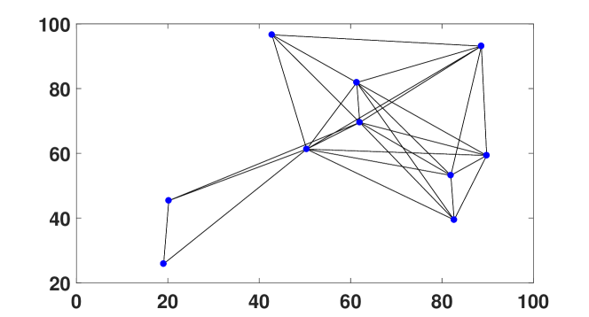
Figure 1: Graph structure for a network of individuals

Simulation for Theorem 1: Choose, for $i\in[10]$, $\beta_{i}^{1}=0.01,\beta_{i}^{w1}=0.01,\delta_{i}^{1}=3$, and, for $j\in[5]$, $\delta_{j}^{w1}=2$. Choose, for $i\in[10]$, $\beta_{i}^{2}=0.3,\beta_{i}^{w2}=0.01,\delta_{i}^{2}=2$, and, for $j\in[5]$, $\delta_{j}^{w2}=1$. Observe that Assumptions 1–4 hold and $\rho(M_{f}^{1})=0.9984<1$, and $\rho(M_{f}^{2})=1.0012>1$. Figure 2 shows that consistent with Theorem 3.1, the average infection level for virus 1 in the network of individuals and that of resources converge to zero; see the blue line and green line, respectively. As an aside, notice that consistent with (Cui et al., 2022, Theorem 3), the dynamics of virus 2 converge to an endemic equilibrium.

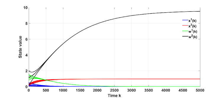
Figure 2: Time-invariant spread dynamics: eradication of virus 1; persistence of virus 2.

Simulation for Corollary 2: Choose, for $i\in[10]$, $\beta_{i}^{1}=0.01,\beta_{i}^{w1}=0.01,\delta_{i}^{1}=3$, and, for $j\in[5]$, $\delta_{j}^{w1}=2$. Choose, for $i\in[10]$, $\beta_{i}^{2}=0.005,\beta_{i}^{w2}=0.01,\delta_{i}^{2}=2$, and, for $j\in[5]$, $\delta_{i}^{w2}=1$. Observe that Assumptions 1–4 hold, and $\rho(M_{f}^{1})=0.9984<1$, $\rho(M_{f}^{2})=0.9994<1$. Figure 3 shows that, consistent with Corollary 2, the average infection level for viruses 1 and 2 in the network of individuals and that of resources converge to zero.

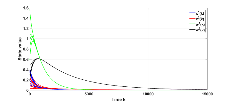
Figure 3: Time-invariant spread dynamics: both viruses get eradicated.

Simulation for Theorem 2: Consider the following sets of values for the system parameters: 1) for $i\in[10]$, $\beta_{i}^{1}(k)=0.01,\beta_{i}^{w1}(k)=0.01,\delta_{i}^{1}(k)=3$, and, for $j\in[5]$, $\delta_{j}^{w1}(k)=2$. For $i\in[10]$, $\beta_{i}^{2}(k)=0.4,\beta_{i}^{w2}(k)=0.01,\delta_{i}^{2}(k)=2$, and, for $j\in[5]$, $\delta_{j}^{w2}(k)=1$. 2) For $i\in[10]$, $\delta_{i}^{1}(k)=0.01,\beta_{i}^{w1}(k)=0.01,\delta_{i}^{1}(k)=3$. for $j\in[5]$, $\delta_{j}^{w1}(k)=2$. For $i\in[10]$, $\beta_{i}^{2}(k)=0.01,\beta_{i}^{w2}(k)=0.01,\delta_{i}^{2}(k)=2$, and, for $j\in[5]$, $\delta_{j}^{w2}(k)=1$. For odd time instants, choose 1) for the parameter values; otherwise, choose 2). Assumptions 1, 6-8 hold and $\sup_{k\in\mathbb{Z}_{\geq 0}}\rho(M_{f}^{1}(k))=0.9984<1$, $\sup_{k\in\mathbb{Z}_{\geq 0}}\rho(M_{f}^{2}(k))=1.0023>1$. Figure 4 shows that the average infection level for virus 1 in the network of individuals and that of resources converge to zero (Theorem 4.3); see the blue line and the green line, respectively. It seems that if the condition is violated, then there exists an endemic equilibrium, to which the infection levels in the network of individuals and the shared resources converge; see the red and black lines, respectively.

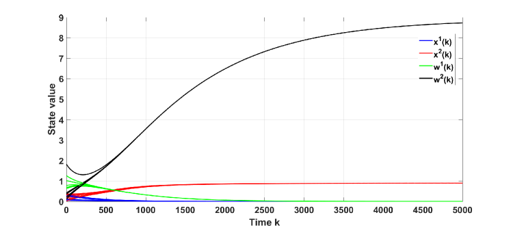
Figure 4: Time-varying spread dynamics with identical healing and infection rates for all individuals: virus 1 gets eradicated, but virus 2 remains persistent.

Simulation for Theorem 3: The network of individuals is partitioned into two groups: Group $a$ (Node 1 – Node 5) and Group $b$ (Node 6 – Node 10). For nodes in group $a$ consider the following choices of parameter values: a1) for $i=1,2,\ldots 5$, $\beta_{i}^{1}(k)=0.1,\beta_{i}^{w1}(k)=0.01,\delta_{i}^{1}(k)=3$, and for $j\in[5]$, $\delta_{j}^{w1}(k)=2$. For $i=6,7,\ldots 10$, $\beta_{i}^{2}(k)=0.4,\beta_{i}^{w2}(k)=0.01,\delta_{i}^{2}(k)=2$, and for $j\in[5]$ $\delta_{j}^{w2}(k)=1$. a2) For $i=1,2,\ldots 5$, $\beta_{i}^{1}(k)=0.05,\beta_{i}^{w1}(k)=0.01,\delta_{i}^{1}(k)=3$, and for $kj\in[5]$, $\delta_{j}^{w1}(k)=2$. For $i=6,7,\ldots 10$ $\beta_{i}^{2}(k)=0.2,\beta_{i}^{w2}(k)=0.01,\delta_{i}^{2}(k)=2$, and, for $j\in[5]$, $\delta_{j}^{w2}(k)=1$. For odd time instants; choose a1); otherwise, choose a2). For nodes in the group $b$, consider the following choices of values for the parameters: b1) For $i=1,2,\ldots,5$, $\beta_{i}^{1}(k)=0.1,\beta_{i}^{w1}(k)=0.01,\delta_{i}^{1}(k)=3$, and, for $j\in[5]$, $\delta_{j}^{w1}(k)=2$. For $i=1,2,\ldots,5$, $\beta_{i}^{2}(k)=0.01,\beta_{i}^{w2}(k)=0.01,\delta_{i}^{2}(k)=2$, and, for $j\in[5]$, $\delta_{j}^{w2}(k)=1$; b2) For $i=6,7,\ldots,10$, $\beta_{i}^{1}(k)=0.05,\beta_{i}^{w1}(k)=0.01,\delta_{i}^{1}(k)=3$, and, for $j\in[5]$, $\delta_{j}^{w1}(k)=2$. For $i=6,7,\ldots,10$, $\beta_{i}^{2}(k)=0.01,\beta_{i}^{w2}(k)=0.01,\delta_{i}^{2}(k)=2$, and, for $j\in[5]$, $\delta_{j}^{w2}(k)=1$. For odd time instants, choose b1); otherwise, choose b2). Assumptions 6-8 hold and $\sup_{k\in\mathbb{Z}_{\geq 0}}\rho(M_{f}^{1}(k))=0.9987<1$, $\sup_{k\in\mathbb{Z}_{\geq 0}}\rho(M_{f}^{2}(k))=1.0023>1$. Further, $\lvert|M_{f}^{1}(k)\rvert|\leq 1.0016$ for all $k\in\mathbb{Z}_{\geq 0}$, and $\sup_{k\in\mathbb{Z}_{\geq 0}}\lvert|M_{f}^{1}(k+1)-M_{f}^{1}(k)\rvert|=0.0005$. Figure 5 shows that, consistent with Theorem 4.4, virus 1 is eradicated; see the blue and green lines, respectively.

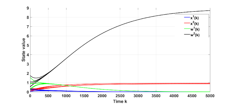
Figure 5: Time-varying spread dynamics with different healing and infection rates for some individuals: virus 1 gets eradicated, but virus 2 remains persistent.

6 Conclusion

The paper studied the spread of multiple competing using a discrete-time time-varying multi-competitive layered networked SIWS model. For time-invariant graphs, we identified a sufficient condition for the exponential eradication of a virus. Thereafter, we established a sufficient condition for exponential eradication of a virus for spread over time-varying undirected graphs with all nodes having identical infection (resp. healing) rates. Finally, for spread over slowly time-varying (un)directed graphs with the nodes not necessarily having identical infection (or healing) rates, we provided a sufficient condition for exponential eradication of a virus. Future work should study the endemic behaviors of the proposed model. Moreover, identifying sufficient (resp. necessary) conditions for estimating the infection level in the population, given knowledge of infection levels in (a part of) the infrastructure network, remains an open problem.

References

- Atkinson (2008) Atkinson, K.E. (2008). An Introduction to Numerical Analysis. John Wiley & Sons.
- Bloom et al. (2018) Bloom, D.E., Cadarette, D., and Sevilla, J. (2018). Epidemics and economics. Finance & Development, 55(002).
- Castillo-Chavez et al. (1989) Castillo-Chavez, C., Hethcote, H.W., Andreasen, V., Levin, S.A., and Liu, W.M. (1989). Epidemiological models with age structure, proportionate mixing, and cross-immunity. Journal of Mathematical Biology, 27(3), 233–258.
- Cui et al. (2022) Cui, S., Liu, F., Jardón-Kojakhmetov, H., and Cao, M. (2022). Discrete-time layered-network epidemics model with time-varying transition rates and multiple resources. arXiv preprint arXiv:2206.07425.
- Desoer (1970) Desoer, C. (1970). Slowly varying discrete system . Electronics Letters, 6(11), 339–340.
- Dunford and Schwartz (1958) Dunford, N. and Schwartz, J.T. (1958). Linear Operators Part I: General Theory. Interscience publishers New York.
- Giordano et al. (2020) Giordano, G., Blanchini, F., Bruno, R., Colaneri, P., Di Filippo, A., Di Matteo, A., and Colaneri, M. (2020). Modelling the COVID-19 epidemic and implementation of population-wide interventions in Italy. Nature Medicine, 26(6), 855–860.
- Gracy et al. (2020) Gracy, S., Paré, P.E., Sandberg, H., and Johansson, K.H. (2020). Analysis and distributed control of periodic epidemic processes. IEEE Transactions on Control of Network Systems, 8(1), 123–134.
- Hertzberg et al. (2018) Hertzberg, V.S., Weiss, H., Elon, L., Si, W., Norris, S.L., Team, F.R., et al. (2018). Behaviors, movements, and transmission of droplet-mediated respiratory diseases during transcontinental airline flights. Proceedings of the National Academy of Sciences, 115(14), 3623–3627.
- Hethcote (2000) Hethcote, H.W. (2000). The mathematics of infectious diseases. SIAM Review, 42(4), 599–653.
- Horn and Johnson (2012) Horn, R.A. and Johnson, C.R. (2012). Matrix Analysis. Cambridge University Press.
- Jackson (2009) Jackson, C. (2009). History lessons: The Asian flu pandemic. British Journal of General Practice, 59(565), 622–623.
- Janson et al. (2020) Janson, A., Gracy, S., Paré, P.E., Sandberg, H., and Johansson, K.H. (2020). Networked multi-virus spread with a shared resource: Analysis and mitigation strategies. arXiv preprint arXiv:2011.07569.
- Johnson and Mueller (2002) Johnson, N.P. and Mueller, J. (2002). Updating the accounts: Global mortality of the 1918-1920 “Spanish” influenza pandemic. Bulletin of the History of Medicine, 105–115.
- Kato (1960) Kato, T. (1960). Estimation of iterated matrices, with application to the von Neumann condition. Numerische Mathematik, 2(1), 22–29.
- La Rosa et al. (2020) La Rosa, G., Iaconelli, M., Mancini, P., Ferraro, G.B., Veneri, C., Bonadonna, L., Lucentini, L., and Suffredini, E. (2020). First detection of SARS-CoV-2 in untreated wastewaters in Italy. Science of The Total Environment, 736, 139652.
- Nowzari et al. (2016) Nowzari, C., Preciado, V.M., and Pappas, G.J. (2016). Analysis and control of epidemics: A survey of spreading processes on complex networks. IEEE Control Systems Magazine, 36(1), 26–46.
- Paré et al. (2020a) Paré, P.E., Gracy, S., Sandberg, H., and Johansson, K.H. (2020a). Data-driven distributed mitigation strategies and analysis of mutating epidemic processes. Proc. 59th IEEE Conference on Decision and Control,, 6138–6143.
- Paré et al. (2022) Paré, P.E., Janson, A., Gracy, S., Liu, J., Sandberg, H., and Johansson, K.H. (2022). Multi-layer SIS model with an infrastructure network. IEEE Transactions on Control of Network Systems.
- Rantzer (2011) Rantzer, A. (2011). Distributed control of positive systems. in Proc. 50th IEEE Conference on Decision and Control and European Control Conference,, 6608–6611.
- Rugh (1996) Rugh, W.J. (1996). Linear System Theory, volume 2. Prentice Hall Upper Saddle River, NJ.
- Santos et al. (2015) Santos, A., Moura, J.M., and Xavier, J.M. (2015). Bi-virus SIS epidemics over networks: Qualitative analysis. IEEE Transactions on Network Science and Engineering, 2(1), 17–29.
- Snow (1855) Snow, J. (1855). On the Mode of Communication of Cholera. John Churchill.
- Van Mieghem et al. (2008) Van Mieghem, P., Omic, J., and Kooij, R. (2008). Virus spread in networks. IEEE/ACM Transactions On Networking, 17(1), 1–14.
- Varga (2000) Varga, R. (2000). Matrix Iterative Analysis. Springer-Verlag.
- Vermeulen et al. (2015) Vermeulen, L., Hofstra, N., Kroeze, C., and Medema, G. (2015). Advancing waterborne pathogen modelling: Lessons from global nutrient export models. Current Opinion in Enviromental Sustainability, 14, 109–120.
- Vidyasagar (2002) Vidyasagar, M. (2002). Nonlinear Systems Analysis. SIAM.
- World Health Organization (2021) World Health Organization (2021). Novel coronavirus (2019-nCoV). https://www.who.int/westernpacific/emergencies/novel-coronavirus. Accessed: 2021-11-15.