Electron-Ion Temperature Ratio in Astrophysical Shocks

Abstract

Collisionless shock waves in supernova remnants and the solar wind heat electrons less effectively than they heat ions, as is predicted by kinetic simulations. However, the values of T_e/T_p inferred from the H$\alpha$ profiles of supernova remnant shocks behave differently as a function of Mach number or Alfvén Mach number than what is measured in the solar wind or predicted by simulations. Here we determine T_e/T_p for supernova remnant shocks using H$\alpha$ profiles, shock speeds from proper motions, and electron temperatures from X-ray spectra. We also improve the estimates of sound speed and Alfvén speed used to determine Mach numbers. We find that the H$\alpha$ determinations are robust and that the discrepancies among supernova remnant shocks, solar wind shocks and computer-simulated shocks remain. We discuss some possible contributing factors, including shock precursors, turbulence and varying preshock conditions.

1 Introduction

Collisional shock waves are characterized by a thickness of order the mean free path. Because the shock transitions are mediated by particle-particle collisions, they produce Maxwellian distributions and thermal equilibrium among the particle species. On the other hand, the thickness of a collisionless shock in a plasma is much smaller, of order the proton gyroradius or ion skin depth. Because they are mediated by electromagnetic fields and plasma turbulence instead of particle collisions, collisionless shocks can produce non-Maxwellian velocity distributions and very different temperatures among different particle species. Except for shocks inside stars or in molecular clouds, most astrophysical shocks are collisionless.

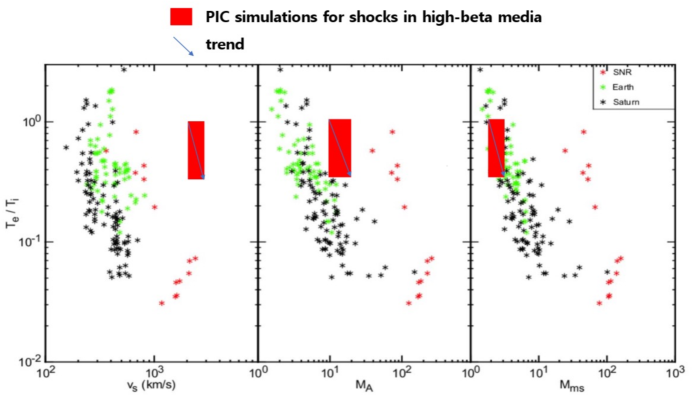
Figure 1: Comparison of estimates of T_e/T_p from SNR shocks and from solar system shocks measured in situ plotted against shock speed, Alfvén Mach number and magnetosonic Mach number, adapted from Figure 7 of Ghavamian et al. (2013). The red boxes and arrows indicate trends from PIC simulations of low Mach number perpendicular shocks in the high $\beta$ plasma typical of galaxy clusters (Ryu et al., in preparation). We expect $\beta$ in the range 0.2 to 2 for most SNR shocks, but the simulation values of T_e/T_p show little dependence on $\beta$.

The electron and proton temperatures T_e and T_p predicted by the Rankine-Hugoniot jump conditions can be very different, because a shock thermalizes most of the kinetic energy of the particles flowing through it, and the electron and ion kinetic energies differ by their mass ratio. Collisions can eventually bring T_e and T_p into equilibrium, but over a time scale that can exceed the dynamical age of the astrophysical object (e.g., supernova remnants, galaxy cluster shocks, structure formation shocks). However, energy dissipation in the shock front and precursor occurs by way of strong plasma turbulence, and this plasma turbulence is capable of transferring energy between ions and electrons more rapidly.

Reliable determination of T_e/T_p is important for understanding the physics of collisionless shocks. For instance, electron-ion thermal equilibration can affect the shock reformation process (Shimada & Hoshino, 2005). T_e/T_p is also important as a diagnostic tool, since T_e is measured from X-ray spectra. In partially neutral preshock conditions, shock speeds can also be determined from the H$\alpha$ line profile, which effectively measures T_p (Chevalier & Raymond, 1978; Bychkov & Lebedev, 1979). In cases where protons keep all the thermal energy, T_p is twice as large as it will be in thermal equilibrium, when half the thermal energy is given to the electrons. Finally, electron heating may play a significant role in the injection of particles into the diffusive shock acceleration process (DSA) which produces radio and X-ray synchrotron emission as well as gamma-ray emission from inverse Compton scattering in SNRs.

Different estimates for the degree of electron-ion temperature equilibration in collisionless shocks give contradictory results. The in situ measurements of bow shocks in the solar wind at Earth and Saturn show T_e/T_p dropping from 1 at very low sonic Mach numbers or Alfvén Mach numbers (M or M_A) to about 0.1 at Mach numbers near 10. Although observations of supernova remnants (SNRs) show a parallel decline, the trend is systematically shifted to much higher Mach numbers. In SNRs, T_e/T_p is near 1 at M$\sim$30, and it drops to 0.05 at M$\sim$300 as shown in Figure 1 (adapted from Ghavamian et al. (2013)).

A second inconsistency arises at higher Mach numbers. Both particle-in-cell (PIC) simulations and solar wind shocks show a drop in T_e/T_p with Mach number between M=1 and M=15, but then T_e/T_p rises to about 0.2-0.3 (Bohdan et al., 2020; Hanusch et al., 2020; Tsiolis et al., 2021; Wilson et al., 2020). On the other hand, values of T_e/T_p from the H$\alpha$ profiles observed in SNR shocks continue to decline with M to about 0.05 at M$\simeq$300 (Ghavamian et al., 2013).

Given the importance of understanding the electron-ion temperature ratio for interpreting observations of SNRs and other shocks, as well as for understanding collisionless shock physics and the acceleration of nonthermal electrons in shock waves, we try to resolve these discrepancies. In principle, the values of T_e/T_p derived from the SNR observations, PIC simulations and in situ measurements could all be correct, but the former pertain to a structure many orders of magnitude thicker than do the latter. The SNR measurements could be appropriate for such tasks as interpreting X-ray spectra, while the in situ and PIC results could be appropriate for studies of plasma processes on small scales. For instance, the PIC simulations and solar wind measurements could pertain to a subshock, while the SNR observations would include any precursor or postcursor effects.

On the other hand, the discrepancies could result from errors in either the theory or observations of the SNRs. In particular, the comparison in Ghavamian et al. (2013) relied on the H$\alpha$ line profiles of shocks in partially neutral gas. The profiles consist of a narrow component from H atoms that are collisionally excited after they pass through the shock, and a broad component from atoms that undergo charge transfer with postshock protons, acquiring a velocity distribution like that of the protons before they are excited (Chevalier et al., 1980). The ratio of the broad and narrow component intensities, I_B/I_N, depends on the electron temperature, and it is often used to determine T_e/T_p. However, this carries some uncertainty.

The aim of this paper is to compare T_e/T_p determinations based on the intensity ratios of the broad and narrow components of the H$\alpha$ profiles of SNR shocks (Ghavamian et al., 2013) with determinations that use electron temperatures measured from X-ray spectra, T_e,x, proton temperatures based on H$\alpha$ broad component widths, T_p,w, and shock speeds based upon proper motions for SNRs at known distances, V_pm. We make four sets of determinations based on 1) I_B/I_N vs broad component H$\alpha$ width, 2) T_p,w vs T_e,x, 3) V_pm vs T_p,w, and 4) V_pm vs. T_e,x, all based on published measurements of the relevant quantities. We will look for common trends of T_e/T_p with shock speed M or M_A among these different estimates.

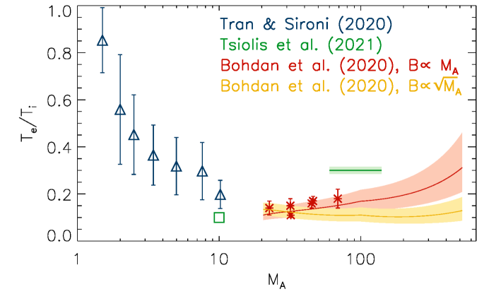
Figure 2: T_e/T_p for perpendicular shocks based on PIC Tran & Sironi (2020) (blue), Bohdan et al. (2020) (red) and Tsiolis et al. (2021) (green). The prediction of Te/Tp at M${}_{A}>$100 depends on the magnetic field generated by the Weibel instability: The red line is for B $\sim$ M_A and the yellow line is for B $\sim$ $M_{A}^{1/2}$ (see updated results in Bohdan et al. (2021)).

We will not attempt a statistical comparison because the uncertainties are dominated by systematic errors in the measurements or the T_e/T_p determinations that we cannot quantify. For example, we try to choose a portion of an SNR shock where V_pm and T_e are both measured, but the values will not always pertain to exactly the same plasma. All the values of the basic parameters are taken from the literature, and when a range of values is given, it indicates the range that entered an average rather than a 1-$\sigma$ or 3-$\sigma$ uncertainty. The comparison is complicated by the fact that we often take, for instance, proper motions from one paper and electron temperatures based on X-ray spectra from another. Detailed considerations for each SNR are given in the Appendix.

The paper is organized as follows. Section 2 describes predictions from numerical simulations, and Section 3 describes results from in situ measurements of shocks in the solar wind and in the laboratory. Section 4 describes the diagnostic measurements of SNR shocks, and section 5 discusses the four methods of estimating T_e/T_p in SNR shocks, along with the uncertainties involved. Section 6 discusses the comparisons among SNRs, solar wind and laboratory shocks and theory. It emphasizes the questions of whether the inclusion of shock precursors or postshock processes, cosmic ray acceleration, or the presence of neutrals in the regions observed in the SNRs can account for the differences. Section 7 summarizes our results, and the Appendix gives details of the T_e/T_p estimates for each SNR.

2 Predictions from Theory and Simulations

Early theoretical calculations for solar wind shocks based on energy transfer by various wave modes or on shock electric fields predicted T_e/T_p$\sim$0.2 (Cargill & Papadopoulos, 1988; Hull & Scudder, 2000). On the other hand, Ghavamian et al. (2007b) attempted to explain the observed decline on T_e/T_p in SNRs with shock speed based on lower hybrid waves in a cosmic ray-generated precursor.

PIC simulations of shocks have explored part of parameter space. For perpendicular shocks in plasma with $\beta$ near 1, T_e/T_p drops steeply from 1 at very small M_A to 0.1-0.2 at M_A = 10 (Tran & Sironi, 2020), then increases slowly from $\sim$0.1 at M_A = 20 to 0.2 at M_A = 100 (Bohdan et al., 2020), and perhaps tends asymptotically to 0.3 at higher M_A (Tsiolis et al., 2021). It should be noted that the prediction for Mach numbers above 100 depends on the scaling with M_A, and the saturation level may drop from 0.3 to 0.1. The results are summarized in Figure 2.

Oblique shocks seem to behave like perpendicular shocks, even in the presence of the electron foreshock generated by the shock reflected electrons (Morris et al., 2023). Lezhnin et al. (2021) report T_e/T_p$\sim$0.5 in a Mach 15 shock at $\Theta_{BN}=60^{\circ}$, where $\Theta_{BN}$ is the angle between shock normal and the magnetic field. On the other hand, parallel shocks are analytically predicted to show a decline in T_e/T_p with Mach number similar to that seen in SNRs, as shown in Figure 12 of Arbutina & Zeković (2021), or to show a decline from near equilibration to around 0.3 at M_A around 20 (Hanusch et al., 2020). Tran & Sironi (2020) investigated low M shocks in the context of the solar wind. That work and subsequent simulations show that at low Mach numbers, the electron heating is not much above that predicted for adiabatic compression, but that the non-adiabatic heating decreases with increasing magnetic obliquity. It increases with Mach number, and neither plasma $\beta$ nor the assumed electron-ion mass ratio is very important.

PIC simulations have also been performed for weak shocks ($M\sim 2-5$) in high beta plasmas ($\beta\gg 1$), as appropriate to shocks that form in hot intracluster medium (ICM) during mergers of galaxy clusters. Electron heating mechanisms and their efficiency were investigated for strictly perpendicular 2D shocks by Guo et al. (2017, 2018) who noted that T_e/T_p is independent of plasma $\beta$ in the range $\beta=4-32$ but decreases strongly with Mach number from T_e/T_p$\sim 0.8$ at $M=2$ to T_e/T_p$\sim 0.25$ at $M=5$. This result should hold at oblique superluminal shocks with $\Theta_{BN}>\Theta_{BN,cr}=\cos^{-1}{(v_{\mathrm{sh}}^{\mathrm{up}}/c)}$. A recent calculation by Kobzar et al. (2021) for an $M=3$ ($M_{A}$=6.1) and $\beta=5$ shock with a subluminal obliquity $\Theta_{BN}=75^{\circ}$, close to $\Theta_{BN,cr}\approx 81.4^{\circ}$ for their parameters, gives T_e/T_p$\sim 0.4-0.45$ in agreement with results by Guo et al. (2018). This is also compatible with 2D PIC simulations presented in Kang et al. (2019a). They found (private communication) that T_e/T_p increases with plasma beta from T_e/T_p$\sim 0.55$ at $\beta=20$ to T_e/T_p$\gtrsim 0.7$ at $\beta=100$ at a subluminal angle $\Theta_{BN}=63^{\circ}$ for an $M=3$ shock. T_e/T_p decreases in their simulations with the Mach number, but can reach T_e/T_p$\gtrsim 1$ in very weak shocks with $M\sim 2$. It also depends quite strongly on $\Theta_{BN}$, and approaches T_e/T_p around 1 at high obliquity angles in very high $\beta$ plasmas.

A limitation of some of the PIC simulations is an unrealistic electron-ion mass ratio. For instance, Shalaby et al. (2022) simulated very fast shocks (40,000 $\rm km~{}s^{-1}$) and found that a mass ratio of 100 suppresses an intermediate-scale instability in low M_A shocks. On the other hand, simulations by Tran & Sironi (2020) (m_i/m_e=20-625) and Bohdan et al. (2020) (m_i/m_e=50-400) demonstrate that the ion-to-electron mass ratio has a minor influence on T_e/T_p if the mass ratio is high enough to separate electron and ion scales (e.g., m_i/m${}_{e}>$100). They indicate that changing shock velocity ratio with respect to c, with Mach and $\beta$ fixed, does not affect this conclusion (Lezhnin et al., 2021)

They indicate that shock velocity does not affect this conclusion as long as all plasma components remain nonrelativistic.

3 Measurements of Shocks in the Solar Wind and the Laboratory

Extensive studies of T_e/T_p in the Earth’s bow shock (Schwartz et al., 1988) and Saturn’s bow shock (Masters et al., 2011) have been conducted, and results are presented in Ghavamian et al. (2013) and in Figure 1. The recent work of Wilson et al. (2020) is based on careful analysis of 15,000 velocity distribution functions in 52 interplanetary shocks seen by the Wind spacecraft. While there is a very large scatter, the average shows the electron heating increasing gradually with M_A, such that for solar wind shocks, T_e/T_p would be expected to drop from 1 at small Mach numbers to $\sim$0.05 at Mach numbers near 10, then rise to around 0.4 at Mach numbers of order 40. They found little correlation with parameters such as pre-shock $\beta$ or shock obliquity.

As with the values of T_e/T_p inferred from SNR observations and the values expected from PIC simulations, there are caveats. In particular, the shocks may not be steady, and the electrons may be mobile enough that they reflect average conditions rather than the local shock parameters, so that measurements from a single spacecraft passing through a shock will not always reflect the expected local electron-ion equilibration.

Recent developments in high-power lasers are now creating important opportunities to probe the plasma microphysics of collisionless shocks in controlled laboratory experiments. The interest in using laser-produced plasmas to study the physics of collisionless shocks is not new. Early experiments in the 70’s and 80’s have used 100 J class lasers to ablate solid targets and produce interpenetrating plasma flows to study their collisionless coupling (Dean et al., 1971; Cheung et al., 1973; Bell et al., 1988). However, for such laser energies, these earlier studies, were limited to relatively low Mach numbers and electrostatic coupling. The development of high-energy laser facilities capable of delivering 10 kJ to MJ laser energy on target, such as OMEGA and the National Ignition Facility (NIF) are transforming the ability to study for the first time high-Mach number collisionless regimes dominated by electromagnetic processes as pertinent to most space and astrophysical shocks.

In the last few years, several experiments produced supersonic, super-Alfvénic plasma flows in the laboratory to study the underlying shock formation processes (Ross et al., 2012; Fox et al., 2013; Huntington et al., 2015; Niemann et al., 2014; Schaeffer et al., 2017; Rigby et al., 2018; Swadling et al., 2020; Fiuza et al., 2020). The plasma flow velocities produced are typically in the range of 500 $\rm km~{}s^{-1}$ to 2000 $\rm km~{}s^{-1}$ and the corresponding Mach number M = 2 - 400. Developments in plasma diagnostics are starting to allow resolved measurements of the evolution of the plasma temperature in these systems. In particular, recent experiments at NIF characterized the formation of a collisionless shock with M $\sim$ 12 and M${}_{A}~{}\sim$ 400, measuring a downstream T_e = 3 keV using Thomson scattering, and demonstrating the acceleration of nonthermal electrons to energy $>$ 100 T_e (Fiuza et al., 2020). While these experiments did not measure T_i, considering that during shock formation the plasma flow velocity varies between 1800 km/s and 1000 km/s (the velocity of the laser produced flows varies in time) and using the standard conservation equations at the shock, one obtains $\rm ZT_{e}/T_{i}=0.15-0.75$ (note that the experiments use carbon plasmas with Z = 6). This is consistent with the PIC results summarized in Fig. 2, which suggest T_e/T_p = 0.1-0.4 for M_A = 400. Planned follow-up experiments will measure simultaneously the electron plasma wave and ion acoustic wave features of the Thomson scattering spectrum (Ross et al., 2012), enabling a detailed characterization of T_e/T_i. Furthermore, by varying the field strength and orientation of an external magnetic field produced by coils it will be possible to study T_e/T_i as function of M, M_A, and $\theta_{BN}$.

Table 1

Equilibration from the H$\alpha$ I_B/I_N

SNR	Pos	Navg	FWHMB	FWHMN	$\rm I_{B}/I_{N}$	VS	Te/Tp	Ref
			$\rm km~{}s^{-1}$	$\rm km~{}s^{-1}$		$\rm km~{}s^{-1}$
SN1006	NW	19	2300-2600	18-24	0.67-0.86	2700-3400	0.09	N13, M12
Tycho	knot ”g”	4	1760-2100	49(250)	0.67-1.08	1850-2400	0.05-0.15	G01, K17, S91, M12
Kepler	-	6	1540-3500	42	0.45-1.1	1250-2700	0.8	S03, B91, M12
RCW 86	SW	1	544-580	36	1.15-1.21	580-620	0.35-0.65	G01, S03
Cygnus Loop	North	9	203-296	35-43	0.60-1.39	300	0.8-1.0	M14, G99
0509-67.5	NE	3	4750-4235	25-31	0.05-0.7	$>$7000	$<$0.25	H18, M12
0519-69.0	-	1	1800-2800	39-42	0.4-0.8	2500	$<$0.20	S91, S94, M12, H18
0548-70.4	-	1	720-800	39-58	0.9-1.3	760	$>$0.5	S91, S94, M12
DEM L71	-	21	450-950	32-43	0.37-0.68	450-950	$>$0.1	S94, R09, M12
1E102.2-7219

References for Tables 1-5: A22- Alan & Bilir (2022), B19-Bandiera et al. (2019), B91-Blair et al. (1991), B06-Borkowski et al. (2006), C22-Coffin et al. (2022), G99-Ghavamian (2000), G00-Ghavamian et al. (2000), G01-Ghavamian et al. (2001), G17-Ghavamian et al. (2017), G22-Guest et al. (2022b), H02-Hwang et al. (2002), H11-Helder et al. (2011), H18-Hovey et al. (2018), K78-Kamper & van den Bergh (1978), K15- Katsuda et al. (2015), K16- Katsuda et al. (2016), K17-Knežević et al. (2017), K21-Knežević et al. (2021), K10-Kosenko et al. (2010), Mi12-Miceli et al. (2012), M12-Morlino et al. (2012), M13-Morlino et al. (2013), M14-Medina et al. (2014), N13-Nikolić et al. (2013), R03-Rakowski et al. (2003), R09-Rakowski et al. (2009), R17-Raymond et al. (2017), S09-Salvesen et al. (2009), S17 - Sano et al. (2017), S16-Schenck et al. (2016), S21-Seitenzahl et al. (2019), S94-Smith et al. (1994), S91 - Smith et al. (1991), S03-Sollerman et al. (2003), W13-Winkler et al. (2013), W16-Williams et al. (2016), W22-Williams et al. (2022), W03-Winkler et al. (2003), W13-Winkler et al. (2013), X19-Xi et al. (2019)

4 Diagnostic measurements

Here we list the 3 diagnostic measurements we will be using. Each measurement has systematic uncertainties. We discuss some of them here, and we will discuss others in more detail in the next section in the context of the specific estimates of T_e/T_p.

Some diagnostics for determining T_e/T_p in SNR shocks rely on the H$\alpha$ profiles. A collisionless shock in partially neutral gas produces a thin filament of emission in H$\alpha$ and other hydrogen lines, because some of the neutral H atoms are excited before they are ionized (Chevalier & Raymond, 1978; Chevalier et al., 1980). The collisionless shock thickness is set by the proton gyroradius or the skin depth, and it is very thin: $\sim 10^{8-10}\rm~{}cm$ for typical ISM magnetic fields and densities. For comparison, the length scale for excitation and ionization of H is of order $10^{15}\rm~{}cm$. The neutrals pass through the collisionless shock without feeling the electromagnetic fields or plasma turbulence, so many of them still have their preshock velocities when they are excited and emit H$\alpha$. On the other hand, some of the neutrals undergo charge transfer reactions with postshock protons. Those neutrals acquire a velocity distribution similar to the proton distribution, though weighted by the charge transfer cross section and the relative velocity (Chevalier et al., 1980; Ghavamian et al., 2001; Heng & McCray, 2007; van Adelsberg et al., 2008; Morlino et al., 2013). Thus the H$\alpha$ profile consists of a broad component, whose FWHM is comparable to the shock speed, and a narrow component, whose FWHM is typically 20-50 $\rm km~{}s^{-1}$  (Sollerman et al., 2003) .

The width of the H$\alpha$ broad component is a direct measurement of T_p in the postshock region, and the narrow component width indicates the temperature in the preshock region. Both widths include any turbulent motion. The turbulence is likely to be significant in a shock precursor (e.g., Bell (2004)). There may be significant turbulence in the postshock region as well. Small scale (kinetic scale) turbulence will decay over a distance much smaller than the size of the H$\alpha$ emitting region, but we discuss turbulence in more detail below. The intensity ratio I_B/I_N depends on the ratio of ionization time to charge transfer time scale, and it therefore depends on the electron temperature (Raymond, 1991; Smith et al., 1991; Laming et al., 1996; Ghavamian et al., 2001).

A second diagnostic is measurement of T_e,x from an X-ray spectrum. That is accomplished by folding a theoretical emission spectrum through the response function of an X-ray telescope and minimizing chi-squared between the model and the observation. To first order, T_e comes from the continuum shape, $\rm e^{(}-h\nu/kT)$, where h$\nu$ is the photon energy and kT is the thermal energy. Several factors can complicate the T_e,x measurement. It is necessary to separate the shocked ISM or CSM gas from shocked SN ejecta, which are heated by a separate reverse shock. The separation requires good spatial resolution, and that is particularly challenging for SNRs in the Magellanic Clouds. We use temperatures from analyses that were specifically meant to pertain to shocked ISM gas. The X-ray emitting plasma is not in ionization equilibrium. Models of shock-heated gas are available, but the ionization timescale is an additional free parameter in the fit. Elemental abundances introduce still more free parameters, because sputtering gradually liberates refractory elements from dust grains in the hot postshock gas. In addition, there are many cases where a single temperature model does not provide an adequate fit, so the T_e,x determination is ambiguous. Finally, in some cases X-ray synchrotron emission contaminates the spectrum of the thermal emission. That being said, observed temperatures of order 1 keV or less are easily distinguished from the higher temperatures that the faster shocks would produce if they were in thermal equilibrium.

The third diagnostic is measurement of the shock speed based on the proper motion of shocks in an SNR whose distance is known, V_pm. Proper motions are mostly measured with H$\alpha$ filaments because they are sharp, and because high spatial resolution can be achieved, for instance by the Hubble Space Telescope (HST). SNR filaments are tangencies of a line of sight to the thin sheet of shock-heated gas (Hester, 1987), so their motion is perpendicular to the line of sight, and the proper motion should correspond to the actual shock speed. However, Shimoda et al. (2015) simulated a SNR shock in an inhomogeneous medium, and they found that the rippled shock front could put some energy into turbulence rather than heat. In their models, comparison of V_pm with T_p could overestimate the energy in cosmic rays or in electron thermal energy by up to 40%. Proper motions can also be measured from the expansion of a remnant in Chandra X-ray images, provided that a long temporal baseline is available and that there are enough point sources in the field for image registration, or from expansion seen in IR images. In many cases, uncertainty in the distance to the SNR is the main limitation. We will consider a few Galactic SNRs whose distances are well-established, along with SNRs in the Magellanic Clouds.

Table 2

Equilibration from H$\alpha$ profile and T_e,x from X-rays

SNR	Pos	Navg	Vs	Tp	Te	TCoul	Te/Tp	Ref
			$\rm km~{}s^{-1}$	keV	keV	keV
SN1006	NW	1	2800	18.3	0.90	0.93	0.05	W13, N13
Tycho
Kepler	K2-K4	3	1250-1850	5.2-7.2	0.68-1.92	1.24-1.60	0.19	B91, K15
RCW 86	SEouter	1	1530	2.3	$<$0.7	$<$0.3	0.1-0.4	H11, M14
Cygnus Loop	North	1	300-325	0.21	0.17	0.10	0.8	M14, S09
0509-67.5
0519-69.0		4	1300-2800	2.9-18.3	1.43	$<$2.2	0.13	S16, H18
0548-70.4	-	1	720-800	1.2	0.42	0.54	$<$0.42	S16, S91
DEM L71	-	7	450-950	0.39-1.72	0.26-0.43	0.5	$<$0.23	R03, A22
1E102.2-7219

The key to the references is given with Table 1.

5 Four T_e/T_p Determinations

Different methods can be used to to determine T_e/T_p depending on the data available. Here we describe four methods, their uncertainties and the trends of T_e/T_p with shock speed.

5.1 H$\alpha$ Line Profiles: Line Width and I_B/I_N

The combination of the broad component line width and the broad-to-narrow component intensity ratio of a Balmer line filament, sometimes called a nonradiative shock, can be used to determine T_e/T_p. This method has the advantage that a single measurement of the H$\alpha$ profile provides both the shock speed and T_e/T_p. It is also attractive because to first order, the profile is determined by just three well-understood atomic rates; the ionization, charge transfer and excitation rates of H I. An unusual aspect of the atomic rates is that excitation and ionization by protons are important for shock speeds above about 1000 $\rm km~{}s^{-1}$. A second unusual feature is that the narrow component neutrals move at 3/4 V_S relative to the postshock protons, so that a 2D integration over the relative velocity distribution weighted by the velocity-dependent cross section is required (Chevalier et al., 1980; Ghavamian et al., 2001; Heng & McCray, 2007; van Adelsberg et al., 2008; Morlino et al., 2013). The asymmetry in the velocity distribution leads to polarization of H$\alpha$ (Laming, 1990; Sparks et al., 2015; Shimoda et al., 2018). The determination of the broad component width and I_B/I_N from the line profile is generally robust unless the spectral resolution is inadequate or the broad component is not Gaussian (Raymond et al., 2010).

There are two potential difficulties involving the narrow line intensity, however. First, most of the excitations to the 3p level produce Ly$\beta$ photons. The branching ratio for H$\alpha$ is 0.12, so a Ly$\beta$ photon will typically convert to H$\alpha$ after about 8 scatterings. In principle the optical depth to the narrow component Ly$\beta$ photons in the upstream direction is effectively infinite, while in the downstream direction it is typically a few (Chevalier et al., 1980; Ghavamian, 2000). This leads to a situation between Case A, where all the Ly$\beta$ photons escape, and Case B, where all the Ly$\beta$ photons are converted to H$\alpha$. The radiative transfer has been computed for various assumed line widths and preshock neutral fractions, and the conversion efficiency seems not to be too sensitive to those parameters (Chevalier et al., 1980; Hester et al., 1994; Ghavamian et al., 2001). However, there can be a broader component to the narrow line (Morlino et al., 2013; Knežević et al., 2017), and the precursor may accelerate the gas away from the preshock rest velocity, which might reduce the efficiency of conversion of Ly$\beta$ to H$\alpha$. It should be noted that I_B/I_N can also depend on the preshock neutral fraction, f₀. Morlino et al. (2013) show results for a reference value f₀ = 0.5. Since f₀ will not generally be much larger than that because of photoionization by He I and He II photons from the shock, and it will not usually be much smaller because that would make the Balmer emission very faint, we use that value. The two exceptions are SN1006, where f₀ is about 0.1 (Ghavamian et al., 2002) and knot ”g” of Tycho, where f₀ may be as large as 0.8 (Ghavamian et al., 2000).

The second potential difficulty is more complex. Gas upstream of a shock will be heated and ionized by ionizing photons from the SNR, and it may produce significant H$\alpha$ emission. Photoionization precursors are likely to be arcminutes thick for Galactic SNRs (Ghavamian et al., 2000; Medina et al., 2014). In principle, emission from such a precursor is subtracted along with the Geocoronal and Galactic H$\alpha$ backgrounds, but it may vary on smaller scales and be difficult to subtract.

There are also precursors associated with cosmic ray acceleration and with broad component neutrals that overtake the shock and deposit their energy upstream (Hester et al., 1994; Smith et al., 1994; Raymond et al., 2011; Morlino et al., 2012; Ohira, 2012). In Galactic SNRs these cosmic ray or neutral return precursors are on the order of arcseconds thick (Lee et al., 2010; Katsuda et al., 2016). Therefore, depending on the size of the region observed and on the seeing, a larger or smaller contribution from the precursor could be present. So far, there are few calculations of the H$\alpha$ emission from the precursor, but Morlino et al. (2012) compute the emission from the precursor and I_B/I_N for shocks faster than 1000 $\rm km~{}s^{-1}$. The precursor not only contributes to the narrow line emission, but ionization within the precursor can reduce the number of neutrals that reach the shock and undergo charge transfer to produce the broad component.

The Morlino et al. (2012) calculations assume Case B, so they somewhat overestimate I_N, and the results depend on the uncertain degree of electron-ion equilibration in the precursor. In addition, Morlino et al. (2012) did not include helium. For very fast shocks, this is appropriate, since there is little temperature equilibration among different ion species, but at lower shock speeds the helium ions can significantly heat the protons (Raymond et al., 2015, 2017). With those caveats, we use Figure 16 of Morlino et al. (2012) to estimate T_e/T_p from I_B/I_N for shocks faster than about 1000 $\rm km~{}s^{-1}$ and Ghavamian et al. (2001) for slower shocks. The contribution of the precursor to the H$\alpha$ narrow component can be assessed to some extent from intensity of associated [N II] emission (Medina et al., 2014).

The resulting estimates of T_e/T_p are shown in Table 1. The columns give the name of the SNR, the position within the SNR if one is given and if the measurement is not averaged over too large a region, the number of positions averaged (N_avg), the broad and narrow component line widths, the broad to narrow intensity ratio, and the shock speed and T_e/T_p derived from those values. The key to the references in this and other tables is included. There is a definite trend of high values of T_e/T_p in shocks slower than about 1000 $\rm km~{}s^{-1}$, while faster shocks show values below about 0.2. This is similar to the results compiled by Ghavamian et al. (2007b).

Table 3

Equilibration from V_pm and T_e,x

SNR	Pos	Navg	PM	D	VSHOCK	Te	TCoul	Te/Tp	Ref
			″/yr	kpc	$\rm km~{}s^{-1}$	keV	keV
SN1006	SE	8	0.50-0.70	1.85	4500-6300	1.60-2.10	0.57	0.02	Mi12
Tycho	west	6	0.28	3	4000	1.7-2.4	0.51	0.027	H02, W16
Kepler
RCW 86	SEouter	1	0.13	2.2-2.6	1530	$<$0.7	$<$0.3	0.1-0.4	H11, M14
Cygnus Loop	North	14	0.069-0.138	0.725	300-470	0.17	0.08-0.16	1.1	S09
0509-67.5
0519-69.0	3	1	0.011	50	1470-3700	1.4	1.9	0.04-0.07	S16, H18, W22
0548-70.4
DEM L71
1E102.2-7219	-	5	0.0055	60	1610$\pm$370	0.66	1.72	0.07-0.24	X19

The key to the references is given with Table 1.

5.2 H$\alpha$ Line Width and T_e,x from X-ray Spectra

This method was used by Rakowski et al. (2003) in a study of DEM L71, where they found that the faster shocks (700-1000 $\rm km~{}s^{-1}$) were consistent with no electron-ion equilibration, while the slower ones (400-600 $\rm km~{}s^{-1}$) were consistent with full equilibration at the shock. This method does not suffer from problems with background subtraction and contributions to the narrow component from a shock precursor. Nor does it depend on the distance to the SNR as the methods that use proper motion velocities do. The method is almost model-independent, it that it uses a direct measure of T_e from X-rays and an almost direct measure of T_p from the H$\alpha$ line width. It is somewhat model dependent in that the H$\alpha$ line width is given by an integral over the charge transfer cross section times the relative velocity distribution (Chevalier et al., 1980), which is further complicated if a particle goes through multiple charge transfer interactions (Heng & McCray, 2007; van Adelsberg et al., 2008; Morlino et al., 2013). Here, for shocks faster than about 1000 $\rm km~{}s^{-1}$ we use the models of Morlino et al. (2013) to infer a shock speed from the line width, then use that shock speed to compute T_p from the Rankine-Hugoniot jump conditions.

The main limitation of this method is that the X-ray spectrum pertains to a relatively thick region behind the shock as compared to the region where the H$\alpha$ line is formed. That means that there is time for Coulomb collisions to transfer energy from ions to electrons, so that the temperature from X-rays is an upper limit to electron heating in the shock itself. If the X-ray temperatures are determined from non-equilibrium ionization (NEI) fits, the product of density times time, $n_{e}t$, is also determined. We use that with the proton temperature and the assumption that the electrons are initially cold to compute T_Coul, the temperature that would be produced by Coulomb collisions alone. In most cases, this is less than the value of T_e determined from X-rays, but not insignificant. In a few cases it is larger than the measured X-ray temperature, indicating a problem with either the temperature or the value of $n_{e}t$ from the fit.

The resulting estimates are shown in Table 2. The electron and proton temperatures from the X-ray spectra and H$\alpha$ profiles, are given, along with the implied shock speed and the value of T_Coul which could be reached by Coulomb collisions alone, and finally T_e/T_p. As with the determinations from the H$\alpha$ profile, there is a clear trend of decreasing T_e/T_p with shock speed from near 1 in the slow shocks in the Cygnus Loop to 0.05 in the fast shocks in SN1006.

5.3 V_pm and T_e,x from X-ray spectra

The shock speed and the Rankine-Hugoniot jump conditions predict the average temperature, so a measurement of T_e implies a value of T_p, and therefore T_e/T_p. We use the jump conditions for positions far upstream and far downstream of the shock. The effects of ionization of neutrals are discussed in Secion 6.1. The main complication is that shocks in an inhomogenous gas become rippled and partly oblique. This can result in a somewhat lower postshock temperature than would be expected from a shock speed derived from the proper motion (Shimoda et al., 2015).

The second complication is that if particle acceleration is efficient, it reduces the thermal energy available. The reduced proton thermal energy can lead to an overestimate of T_e/T_p. The shocks we discuss here do not accelerate particles very efficiently based on a lack of synchrotron X-ray emission at the positions we consider, though other sections in some of the SNRs do have synchrotron X-ray filaments. Many do produce nonthermal radio and gamma-ray emission, in some cases by reacceleration of existing cosmic rays (Tutone et al., 2021). Here, we assume that cosmic rays absorb a negligible fraction of the shock energy, and we return to that assumption in the discussion section, where we summarize estimates of the fractions of shock energy in cosmic rays.

We consider the rather slow shocks in the Cygnus Loop (300-400 $\rm km~{}s^{-1}$; Salvesen et al. (2009)), faster shocks in SN1006 ($\sim 5000$ $\rm km~{}s^{-1}$; Miceli et al. (2012)), and shocks in Magellanic Cloud supernova remnants, where proper motions show speeds of 1400-3700 $\rm km~{}s^{-1}$ (Hovey et al., 2018; Xi et al., 2019; Williams et al., 2018) and electron temperatures have been measured in the outermost regions of the forward shocks chosen to exclude emission from the ejecta (Schenck et al., 2016).

We note that, as for the T_e,x vs. T_p from the H$\alpha$ line width method, the measurement of T_e pertains to a region that is around $10^{17}~{}\rm cm$ or more thick, so that Coulomb collisions can transfer a significant amount of heat from protons to electrons. Therefore, we again include T_Coul in Table 3, an estimate of T_e that would be reached by Coulomb collisions alone if the electrons were initially cold.

Table 3 shows the proper motion shock speeds, the electron temperatures derived from X-rays, the temperatures that would be reached by Coulomb collisions alone, and T_e/T_p. Again, the trend of T_e/T_p decreasing with Mach number is similar to that obtained from I_B/I_N.

5.4 V_pm vs T_p from H$\alpha$ broad component

Some reliable shock speeds have been obtained from measured proper motions and SNR distances, along with H$\alpha$ profiles. The Rankine-Hugoniot jump conditions predict the total thermal energy, and since the proton temperature can be inferred from the H$\alpha$ broad component width, we can determine T_e/T_p. As discussed above, the H$\alpha$ broad component width is not exactly the same as the proton thermal width, but it is determined by integrating over the cross section times the relative velocity of the neutrals and protons (Chevalier et al., 1980; Heng & McCray, 2007; Morlino et al., 2013). Especially at shock speeds above 2000 $\rm km~{}s^{-1}$, the line width is smaller than the proton thermal width. Therefore, we use V_pm the models of Morlino et al. (2013) to derive T_p from the H$\alpha$ width.

Table 4

Equilibration from V_pm and T_p from H$\alpha$ width

SNR	Pos	Navg	PM	D	Vpm	VFWHM	Te/Tp	Ref
			″/yr	kpc	$\rm km~{}s^{-1}$	$\rm km~{}s^{-1}$
SN1006	NW	11	0.37-0.45	1.85	3000	2900	$<$0.1	N13, W03, R17
Tycho	knot ”g”	1	0.20	2.3-3.7	$>$2200	1800	$<$0.4	K78, G01
Kepler
RCW 86	SEouter	1	0.13	2.2-2.6	1530	1120	0.1-0.4	H11, M14
Cygnus Loop	N	3	0.069-0.11	0.725	300-360	203-347	1.0	S09, M14
0509-67.5	NE	3	0.029	50	6900	7800	$<$0.1	H18, M13
0519-69.0	2-S	1	0.011	50	2300-3300	3200-4000	$<$ 0.20	H18, M13
0548-70.4
DEM L71
1E102.2-7219

The key to the references is given with Table 1.

Table 4 gives the proper motions and inferred shock speeds, along with the FWHM of the broad H$\alpha$ component and T_e/T_p. Once again, T_e/T_p tends to decline with shock speed, from approximatedly 1 for the $\sim$400 $\rm km~{}s^{-1}$ shocks in the Cygnus Loop to less than 0.1 in shocks faster than 3000 $\rm km~{}s^{-1}$ in SN1006 and 0509-67.5.

5.5 Evidence from other Observations

Ultraviolet spectra are only available for a few SNRs, but they support the estimates of T_e/T_p given above. First, Laming et al. (1996) used the intensity ratios in SN1006 to show that T_e/T_p$<$0.05. Second, kinetic temperatures of H, He, C, N and O have been measured in a handful of SNRs that are observable in the UV and in H$\alpha$ (Raymond et al., 1995; Korreck et al., 2004; Ghavamian et al., 2007a; Raymond et al., 2015, 2017), as well as X-rays (Miceli et al., 2019). They show fairly complete equilibration in the Cygnus Loop, where the shocks are around 350 $\rm km~{}s^{-1}$, and mass proportional temperatures (no equilibration) in SN1006, where the shocks are faster than 2500 $\rm km~{}s^{-1}$. It is possible that the wave modes responsible for sharing energy between electrons and ions could be different from those that redistribute energy among the different ion species. However, the drop in ion-ion thermal equilibration seems to mirror that in electron-ion equilibration.

Another estimate of T_e/T_p is given by Matsuda et al. (2022), who find T_e/T_p $<$ 0.15 in a knot on the NW limb of Tycho based on the X-ray temperature increase over 15 years and a shock speed of $>$ 1500 $\rm km~{}s^{-1}$. There is also an estimate of T_e/T_p for the reverse shock in Tycho by Yamaguchi et al. (2014), who used the centroid of the Fe K$\alpha$ line to determine the ionization state of iron. They found 0.003 $\leq$ T_e/T_p $\leq$ 0.02 for the reverse shock. Most recently, Ellien et al. (2023) were able to separate thermal from non-thermal X-ray emission at five positions in the South, West and Northeast regions of Tycho, and the 2.0-2.6 keV electron temperatures they derive are much less than the 10-15 keV predicted from the shock speeds of Williams et al. (2016) and the assumption of equal electron and ion temperatures. That indicates that shocks that produce strong synchrotron X-rays also show T_e/T_p$<$ 0.1 of the energy going into cosmic rays and magnetic field amplification is not too large (see Section 6.2).

We also note that, while Table 1 presents numbers for a 600 $\rm km~{}s^{-1}$/ shock in RCW86 from Ghavamian et al. (2001), which was analyzed in the greatest detail, several other positions in RCW86 were presented in Ghavamian (2000). Excluding 3 positions contaminated by radiative shocks, there were 6 other positions whose line widths and I_B/I_N ratios were similar to those in the one in Table 1, so they would have similar shock speeds and values of T_e/T_p around 0.5. There were also 2 positions showing line widths of 325 $\rm km~{}s^{-1}$and I_B/I_N= 1.0$\pm$0.2, indicating shock speeds of around 350-400 $\rm km~{}s^{-1}$ and T_e/T_p $>$ 0.6. These faster shock positions are in good agreement with the RCW86 value shown in Table 1, while the slower shocks agree with the Cygnus Loop value. Overall, these additional points support the trends in Table 1 and Figure 3.

This paper has concentrated on shocks in SNRs, but pure Balmer line spectra are also observed in the bow shocks driven through the ISM by some pulsars. Romani et al. (2022) measured an H$\alpha$ profile in the bow shock of PSR J1959+2048. The shock speed is probably about 150 $\rm km~{}s^{-1}$, but it is not well determined. The I_B/I_N ratio is about 4, which would indicate a low value of T_e/T_p, probably less than 0.2. This is much different than the Cygnus Loop shocks, where I_B/I_N is about 1. One possible cause of this difference is emission from a precursor in the Cygnus Loop. Another is that the T_e/T_p is lower in the bowshock because it is slower. Other possible causes include that the lower temperature in the bow shock favors excitation to the 3s and 3d levels of hydrogen as opposed to 3p and that the smaller width of the broad component permits some conversion of Ly$\beta$ to H$\alpha$ in the broad component. The latter might make T_e/T_p as high as 0.5 consistent with I_B/I_N = 4. If the shock speed is significantly less than 150 $\rm km~{}s^{-1}$, the lower postshock temperature would reduce the ionization rate, which could strongly increase I_B/I_N. Since the shock is oblique, the effective shock speed could be smaller than 150 $\rm km~{}s^{-1}$.

6 Discussion

All four estimates of T_e/T_p in SNRs agree that the electron-ion temperature ratio declines sharply with shock speed. The discrepancies between SNR observations and solar wind measurements appeared when T_e/T_p was plotted against V_S, M_A or M_ms in Figure 1, which is adapted from Figure 7 of Ghavamian et al. (2013). Measurements at the bowshocks of Earth and Saturn appeared to disagree when plotted against V_S, but agreed nicely with each other when plotted against M_A or M_ms, while the discrepancy with SNR shocks was magnified by plotting against M_A or M_ms.

The plots just described assumed generic sound speeds and Alfvén speeds for the SNRs of 11 $\rm km~{}s^{-1}$ and 9 $\rm km~{}s^{-1}$, respectively. Here, we consider the possibility that electron heating occurs only in the narrow collisionless shock, while protons are also heated in the precursor. In that case, the relevant sound speed is the sound speed in the precursor, which is given by the narrow line width, rather than the sound speed in the ambient ISM. Therefore, we use the widths of the H$\alpha$ narrow components to determine temperatures and sound speeds. Because nearly all of the observed shocks are Balmer line filaments, we assume that the gas is 50% ionized, except for SN1006 and 1E102.2-7219, which have low neutral fractions. As shown in Table 5, the narrow component widths vary, and the corresponding temperatures range from T₄ = 1.0 to 4.6, where T₄ = T/10,000 K. We note that Tycho’s SNR shows both a narrow and an intermediate component that account for 35% and 65% of the ‘narrow’ component. We have taken the weighted average of the corresponding temperatures in quadrature.

The Alfvén speed is even more problematic, given that neither the ambient magnetic field nor the compression in the precursor is known. For Milky Way SNRs we assume a field strength of 10 $\mu$G (Sofue et al., 2019). Kepler’s SNR and RCW 86 are expanding into their own circumstellar shells, which could have very low magnetic fields or very high fields due to compression, and the preshock densities vary enormously around their peripheries. For lack of reliable numbers, we do not compute Alfvén or magnetosonic speed for those remnants. For the LMC and SMC we also assume 10 $\mu$G based upon Mao et al. (2012), Seta & Federrath (2021), Seta et al. (2022) and Livingston et al. (2022). These are, of course, average magnetic fields, so the local field will be different. To obtain Alfvén speeds, we use preshock densities generally derived from X-ray observations and an assumed compression ratio of 4 at the shock. As seen in Table 5, the preshock densities vary by over an order of magnitude. The Alfvén speed may change in the precursor, but as the plasma and the perpendicular component of the field are compressed together, the change in V_A should not be drastic.

Table 5

Sound Speed and Alfvén Speed

SNR	Pos	V	FWHMnarrow	T4	n0	CS	VA	Ref
		$\rm km~{}s^{-1}$	$\rm km~{}s^{-1}$	104 K	$\rm cm^{-3}$	$\rm km~{}s^{-1}$	$\rm km~{}s^{-1}$
SN1006	Avg	3000	22	1.0	0.1	16	63	B19
Tycho	knot ”g”	2200	49,188	28.	1.0	65	20	K17, G00
Kepler	Avg	2000	42	3.5	-	23	-	S03
RCW 86	SW	560	36	2.6	-	20	-	S03, S17
Cygnus Loop	Avg N	320	35	2.5	0.20	20	44	M14, S09
0509-67.5	Avg	6000	28	1.6	0.4	16	31	S91 S21
0519-69.0	Avg	2500	40	3.2	1.5	22	16	S94, K10, W22
0548-70.4	Avg E	760	48	4.6	0.4	26	31	S91, S94, B06
DEM L71	Avg	800	37	2.8	0.6	21	26	S94, B06
1E102.2-7219	Avg	1600	-	1.0	1.6	12	16	X19

The key to the references is given with Table 1.

Based on the estimates of sound speed and Alfvén speed in Table 5 and the values of T_e/T_p in Tables 1-4, we plot in Figure 3 the equilibration as a function of shock speed, sonic Mach number, Alfvén Mach number and magnetosonic Mach number, using different colors for the different methods of estimation. To reduce the clutter, we plot only a single point for each SNR for each method of estimation, generally an average if a range of values is present, but in some cases such as RCW 86, the best determination for that SNR. We also introduce slight shifts along the X-axis in cases where a symbol in one color would cover that in another color.

Figure 3 shows that the trends of T_e/T_p with shock speed shown in Figure 7 of Ghavamian et al. (2013) (our Figure 1) hold, but that the Mach numbers are considerably smaller. This is due to the generally higher temperatures assumed here based on the narrow component line widths, to the generally higher Alfvén speeds due to smaller preshock density estimates, and to an assumed 10 $\mu$G magnetic field. However, the changes in Mach number, Alfvén Mach number and magnetosonic Mach number are not nearly enough to bring the SNR results into agreement with the solar wind results (T_e/T_p$\sim$0.15 at V$\sim$400 $\rm km~{}s^{-1}$, M${}_{A}\sim$10, M${}_{MS}\sim$7), or with the PIC prediction that T_e/T_p rises to about 0.1 to 0.3 when M_A exceeds about 20 to 30.

There are, or course, still ways in which our Mach numbers could be overestimates. For very short period Alfvén waves, the density of the ionized gas rather than the total density should be used. The ionization fraction is about 90% in SN1006 (Ghavamian et al., 2002), and it cannot be much less than about 0.5 because the shock itself produces ionizing photons (Medina et al., 2014). We also use mean magnetic fields to estimate the Alfvén speed, and the local fields can be higher or lower. We also use the pre-shock temperature estimated from the narrow component line width, and it is possible that protons are further heated in the precursor after the last charge transfer (on average) communicates the proton temperature to the neutrals. It is unlikely that these effects would reduce the Mach numbers by more than a factor of 2.

We therefore consider some ways in which the comparison among SNR, solar wind and PIC simulated shocks might be comparing different things. Then, we consider possible differences in the physics.

6.1 Different Length Scales

One obvious difference between observations of SNR shocks, the measurement of solar wind shocks and the PIC simulations is the scale. The latter two pertain to a few hundred times the ion skin depth, which is on the order of $10^{8}$ cm in the interstellar medium. The H$\alpha$ profile in an SNR shock is formed over an ionization length scale, typically $10^{15}$ cm, and X-ray spectra are generally resolution-limited to scales of $10^{17}$ cm. Thus if a shock has a precursor (either a cosmic ray modified shock or a return neutral precursor), the solar wind and PIC results might pertain to the subshock, while the SNR results pertain to the entire structure. Similarly, if postshock cooling or other processes affect the plasma between the shock jump and the H$\alpha$ formation region, that could affect the comparison. The comparison of laboratory experimental data with SNR observations suffers from similar challenges due to the small scales of the shock evolution captured in the experiments. Nevertheless, laboratory experiments can play an important role in benchmarking the results of numerical simulations, which have sometimes been limited by reduced mass ratios and dimensionality. This will strengthen the understanding of the plasma microphysics and its connection to T_e/T_p in collisionless shocks.

Cosmic ray precursor: A cosmic ray precursor requires magnetic turbulence to reflect accelerating particles back toward the shock, but it is uncertain how effectively the turbulence dissipates or whether it heats ions or electrons more effectively (Morlino et al., 2012). The magnetic turbulence in the precursor will contribute to the narrow component line width, causing an overestimate of the proton temperature and sound speed and an underestimate of the sonic Mach number. By the same token, the narrow component width provides an upper limit on the level of turbulence in the precursor, which is related to the amplification of magnetic fields discussed below.

Return neutral precursor: As was mentioned in connection with the narrow component flux, a neutral return precursor, in which some of the broad component neutrals overtake the shock front and deposit their energy upstream, is also expected (Hester et al., 1994; Raymond et al., 2011; Morlino et al., 2013). When a neutral overtakes the shock, it has at least the average energy of the shocked protons, and when it is ionized by charge transfer or by collision with an electron, it becomes a pickup ion similar to those seen in the solar wind, but with an energy of 0.5 to 200 keV for the shock speeds considered here. The pickup ions tend to be swept back through the shock, and what fraction of their energy is deposited upstream is a complex question. In a perpendicular shock with modest magnetic turbulence, the pickup ions form a ring beam in velocity space, and that very quickly scatters into a bispherical shell distribution in velocity space (Williams & Zank, 1994; Isenberg & Lee, 1996), transferring some of the kinetic energy to Alfvén waves in the process. The amount of energy deposited depends on $\Theta_{BN}$, the plasma $\beta$ and on the neutral fraction (Raymond et al., 2008). It is likely that protons are heated more effectively than electrons, but at the low temperatures in the precursor, Coulomb collisions may transfer energy to the electrons.

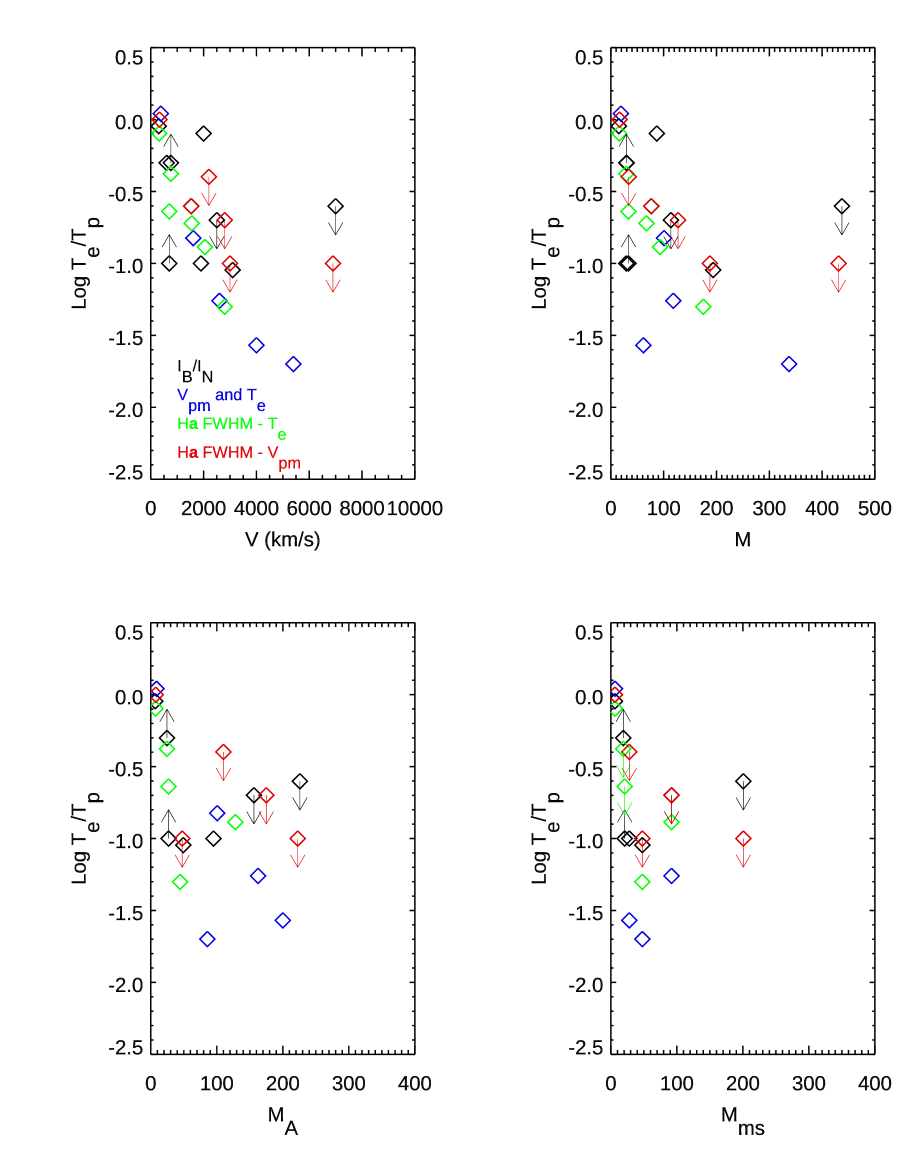
Figure 3: Four estimates of Log T_e/T_p plotted against shock speed, sonic Mach number, Alfvén Mach number and magnetosonic Mach number. At most one value is given for each SNR for each method of estimations, and it is either an average or the best-determined value, as discussed in the Appendix. The estimation method for T_e/T_p is indicated by the color. Note that the X-axis scales are different.

Postshock electron heating and cooling: Another possible factor is that electrons are cooled behind the shock. Some energy is required to ionize the atoms, and some energy is lost by radiation over the region where the Balmer lines are produced, mostly in the form of H I Lyman lines and He I and He II emission lines. The ionization and radiative loss energies involved could cool the electrons by removing thermal energy, but the amount is equivalent to reducing the effective shock speed to $v^{\prime^{2}}=v^{2}-72^{2}$ ($\rm km~{}s^{-1}$)² for a shock in fully neutral gas (Cox & Raymond, 1985), and that is negligible for the shocks we consider here. In addition, ionization of neutrals also liberates electrons, so the thermal energy that electrons gain at the shock is shared among more particles. The neutral fraction can be as high as 50% if there are no sources of ionizing radiation in the neighborhood other than the shock itself, so the liberation of neutrals downstream could cool the electrons to half their value at the shock. That could be a significant factor for the SNRs showing T_e/T_p$\sim$ 0.5, such as RCW 86 or 0548-70.4. The SNR with the most reliably known preshock neutral fraction is SN1006, where only 10% of the hydrogen is neutral (Ghavamian et al., 2002), and there the electrons created by ionization downstream would have only a 10% effect on the temperature. Another possible cooling process is adiabatic expansion, but that would tend to occur on large scales, over which Coulomb collisions could heat the electrons.

Another possible mechanism for heating the electrons downstream is the cosmic ray postcursor discussed by Diesing & Caprioli (2021) and Wilhelm et al. (2020). Here, magnetic turbulence in the postshock region is maintained for a thickness comparable to that of the cosmic ray precursor. If that turbulence is dissipated by reconnection, it could preferentially heat the electrons. That could help to explain why SNR shocks at Mach numbers around 10-15 show substantial equilibration, but it would aggravate the discrepancy between PIC predictions and SNR observations of T_e at high Mach numbers. The energy available is discussed below in connection with cosmic rays.

6.2 Jump Condition Energetics; Cosmic Rays and Magnetic Fields

The T_e/T_p estimates based on V_pm rely on the shock jump conditions and the differences between the inferred total thermal energy and the thermal energies measured for either protons or electrons. With the exception of the analyses of RCW 86 by Morlino et al. (2014) and 0509-67.5 by Hovey et al. (2018), most of these estimates assume that the fractions of shock energy going into cosmic rays and amplification of magnetic fields, $\epsilon_{CR}$ and $\epsilon_{B}$, are small. If the energy in cosmic rays and magnetic fields is significant, it will affect each estimate of T_e/T_p in a different way. The energy to accelerate cosmic rays comes from the protons, since they carry almost all the kinetic energy that is dissipated.

The estimates of T_e/T_p based in I_B/I_N and on the X-ray spectrum vs. the H$\alpha$ line width rely on direct measures of T_e and T_p, so they do not depend on assumptions about the fraction of energy in cosmic rays, but the shock speed would be underestimated by a factor $(1-\epsilon_{CR}-\epsilon_{B})^{1/2}$. The estimate obtained by comparing $T_{e,x}$ with the proper motion shock speed assumes that the ions have all the dissipated shock energy that is not in the electrons, so that T_p is overestimated and T_e/T_p is underestimated if $\epsilon_{CR}$ is significant. The estimate based on comparing T_p from the H$\alpha$ width with V_pm assumes that all the dissipated shock energy that is not in the ions is in the electrons, so it overestimates T_e and T_e/T_p if $\epsilon_{CR}$ is important.

If SNRs provide much of the energy in cosmic rays, then the fraction of shock energy in cosmic rays must be $\epsilon_{CR}$ = 0.05-0.10 (Strong et al., 2010) on average, though $\epsilon_{CR}$ may be much larger in fast shocks than in slower ones (Blasi et al., 2005). We only have detailed estimates for a few SNRs. Tutone et al. (2021) find that $\epsilon_{CR}$ is only about 0.02 in the 400 $\rm km~{}s^{-1}$ nonradiative shocks in the Cygnus Loop. Hovey et al. (2018) find upper limits $\epsilon_{CR}<0.07/(1-f_{0})$ and $\epsilon_{CR}<0.11/(1-f_{0})$, where $f_{0}$ is the preshock neutral fraction, in 0509-67.5 and 0519-69.0, respectively, with shock speeds spanning 1700 to 8500 $\rm km~{}s^{-1}$. Morlino et al. (2014) studied a 1500 $\rm km~{}s^{-1}$ shock in RCW 86, and found 0.05 $<~{}\epsilon_{CR}~{}<0.30$. With the possible exception of some positions in Tycho’s SNR, none of the regions studied here show nonthermal X-ray emission. Therefore, it is unlikely that $\epsilon_{CR}$ is more than 10% in the regions we consider. The recent work of Ellien et al. (2023) determined electron temperatures in Tycho’s SNR shocks by separating the thermal and nonthermal components of the X-ray spectra. Their comparison with temperatures determined from proper motion shock speeds indicates that T_e/T_pis 0.09-0.13 for $\epsilon_{CR}=\epsilon_{B}=0.1$. Thus shocks that produce X-ray synchrotron filaments seem not be behave much differently from shocks that do not.

Cosmic ray acceleration is accompanied by turbulent amplification of the magnetic field. That can reduce the energy available, but it also provides a nonthermal component to the line width. It has generally been assumed that kinetic scale turbulence would damp out over a length much smaller than the thickness of the region where H$\alpha$ forms, but a postcursor in which cosmic rays and turbulence exchange energy is also possible (Wilhelm et al., 2020; Diesing & Caprioli, 2021). The energy in magnetic turbulence could reach equipartition with the cosmic ray energy, $\epsilon_{B}=\epsilon_{CR}$, so it could be as much as 10% of the energy dissipated in the shock. It would reduce T_p like the cosmic rays, but it would increase the H$\alpha$ line width. In the reference case of $\epsilon_{B}=\epsilon_{CR}$ = 0.1, the energy density in the waves is 1/8 the thermal energy density. For Alfvén waves, the magnetic and kinetic energy contributions are equal, so the wave kinetic energy is 1/16 the thermal energy, and if T${}_{p}>>$ T_e the wave velocity amplitudes are 1/4 the proton thermal velocities. If T_p = T_e, the wave velocity contribution would be $\surd 2$ times higher. However, the slow Cygnus Loop shocks where T_p = T_e show $\epsilon_{CR}$ = 0.02 rather than 0.1 (Tutone et al., 2021). If the wave velocity and thermal velocity add in quadrature, the H$\alpha$ line widths are only increased by a few percent. The compilation by Reynolds et al. (2021) indicates that $\epsilon_{B}$ is about 10% on average for Tycho and RCW 86, but those estimates pertain to the X-ray synchrotron filaments rather than the ones studied here. The values of $\epsilon_{B}$ from Reynolds et al. (2021) are much smaller for SN1006 and Kepler.

6.3 Other Parameters

Other shock parameters might influence T_e/T_p. The angle between the shock normal and the magnetic field, $\Theta_{BN}$, could well have an effect according to PIC simulations, as discussed in Sections 2 and 3. There is no reason to believe that the SNR shocks are preferentially either quasi-parallel or quasi-perpendicular, though our avoidance of shocks with X-ray synchrotron emission might bias our sample toward perpendicular shocks according to some models. The ratio of gas pressure to magnetic pressure, $\beta$, could perhaps have an effect, but the preshock values of $\beta$ should be of order 0.1-1, and the solar wind shocks should be roughly similar. As also discussed in section 2, the plasma $\beta$ seems to have little effect for the modest Mach number shocks, and its importance would be expected to be even smaller in faster shocks.

Subcritical/Supercritical shocks: One aspect of the shocks that we have not discussed is their subcritical/supercritical character. Shocks up to M${}_{ms}\sim$2.76 (depending on shock parameters) can dissipate energy efficiently enough to make a smooth, steady shock structure possible (Treumann, 2009). Faster shocks must be unsteady, and reflection of protons at the shock can generate modified two-stream instabilities (MTSI) that produce plasma waves that could couple electrons and ions (Wu et al., 1984). While a supercritical shock may be required to produce some of the wave modes that can transfer energy from electrons to ions, even laminar shocks can produce whistler wave precursors that could transfer energy (Gary & Mellott, 1985). The supernova remnant shocks discussed here are well above the range of subcritical shocks, with the possible exception of the Cygnus Loop shocks, which could perhaps be slower than the “second whistler critical Mach number” or the “third or nonlinear whistler critical Mach number”, allowing phase-standing whistlers to create a steady structure (Kang et al., 2019). In any case, very weak shocks should converge on T_e/T_p$\sim$1 at M$\sim$1 due to adiabatic compression even without electron-ion coupling (Vink et al., 2015). However, the Cygnus Loop electrons are much too hot for adiabatic heating to account for T_e.

Effects of neutral atoms: The most likely parameter to influence electron heating could be the neutral fraction, which is effectively zero in the solar wind and in the PIC simulations, but is 0.1 or more in the Balmer filaments. Neutrals could damp plasma waves and perhaps weaken those responsible for transferring energy from ions to electrons. In general, that is expected to happen for relatively long period waves that resonate with highly energetic particles, so that a significant neutral fraction limits the maximum cosmic ray energy (Reville et al., 2007), while the ion-neutral damping length is much larger than the wavelengths of waves that would interact with thermal particles. If the presence of neutrals is important, it would affect all the T_e/T_p determinations that involve the H$\alpha$ profile. It would not affect the values of T_e/T_p determined by comparing proper motion shock speeds with X-ray determined temperatures in the western side of Tycho or in E0102.2-7219, where no Balmer filaments are seen.

7 Summary

We have used used four measured parameters of SNR shocks to determine T_e/T_p; the H$\alpha$ broad component widths, the H$\alpha$ broad-to-narrow intensity ratios, the electron temperatures derived from X-ray spectra and the shock speeds derived from proper motions. They provide four distinct estimates of T_e/T_p whose systematic uncertainties are different, and we have discussed the uncertainties for each method. We have used published values for the measured parameters, though in some cases we reinterpreted the data using newer models (Morlino et al., 2012, 2013) or newer distances to individual SNRs.

The result is that the trend of T_e/T_p obtained from the H$\alpha$ profiles by Ghavamian et al. (2013) is robust, and the disagreements with measurements of solar wind shocks remain, along with disagreement with PIC simulations. First, the in situ measurements and PIC simulations indicate that T_e/T_p is close to 1 at very low M numbers, but drops to $\sim$ 0.2 around M_A near 15, while the SNR shocks are still at T_e/T_p near 1 at M = 15-25. Second, both PIC simulations and in situ measurements indicate that as the shock speed increases for M above about 20, T_e/T_p increases to about 0.1 to 0.3, while in the SNR shocks, T_e/T_p continues to decrease to 0.05 or less.

We consider several possible avenues to resolve this discrepancy: the scale lengths of the regions where the diagnostic emission is formed, the presence of energetic particles and magnetic turbulence, the roles of shock precursors and postcursors, the Alfvén speeds used to derive Alfvén Mach numbers, and the presence of neutrals. While some of these factors decrease the discrepancies, they do not provide definitive explanations.

Thus, we have utterly failed to resolve the discrepancies among SNR shocks, solar wind shocks, and PIC simulations in electron-ion thermal equilibration. It is not clear whether the answer lies in more theory or more observations. Systematic observational studies, in which H$\alpha$ profiles, proper motion measurements and high resolution UV and X-ray spectra of individual shocks are obtained, are needed. On the theoretical side, simulations that include neutrals and the important plasma processes are needed, both upstream and downstream of the shock jump.

8 Acknowledgements

This research was supported by the International Space Science Institute (ISSI) in Bern, through ISSI International Team project #520. The effort was supported by HST Guest Observer grant GO-15285.0001_A to the Smithsonian Astrophysical Observatory. The work of J. N. has been supported by Narodowe Centrum Nauki through research project No. 2019/33/B/ST9/02569. The work of DR was supported by the National Research Foundation of Korea through 2020R1A2C2102800. AT was supported by NASA grant FINESST 80NSSC21K1383. AB was supported by the German Research Foundation (DFG) as part of the Excellence Strategy of the federal and state governments - EXC 2094 - 390783311.

Appendix A SN 1006

SN1006 has been extensively studied. H$\alpha$ is present around the entire circumference, but it is too faint for good line profiles to be obtained except in the NW, where Nikolić et al. (2013) obtained excellent IFU data. Proper motions have been measured both in H$\alpha$ and X-rays (Winkler et al., 2003; Miceli et al., 2012; Katsuda et al., 2013; Raymond et al., 2017). The distance to SN1006 has been estimated in a number of ways to be 1.6-2.2 kpc. High velocity absorption from the unshocked ejecta of SN 1006 has been seen in the spectrum of the Schweizer-Middleditch star, whose Gaia parallax indicates 1.43-2.0 kpc. A distance less than 1.6 kpc would imply shock speeds too small to account for the observed H$\alpha$ line widths. Therefore, we adopt D = 1.85$\pm$0.15 kpc to convert proper motions to shock speeds. X-ray temperatures are taken from Winkler et al. (2013) in the NW and Miceli et al. (2012) in the SE. We note that the regions observed by Miceli et al. (2012) do not show the relatively bright H$\alpha$ seen in the NW, but very faint H$\alpha$ is present. That might indicate a neutral fraction even lower than the value of 0.1 in the NW found by Ghavamian et al. (2002). Miceli et al. (2012) found values of n_et of only 2-7$\times 10^{8}~{}\rm cm^{-3}~{}s$, so T_Coul is only about 1/3 the observed X-ray temperatures. In the NW, Winkler et al. (2013) find a higher value of n_et, so Coulomb collisions could provide a substantial fraction of the temperature obtained from the X-ray spectra. We also note that other measurements of T_e,x and V_pm yield similar results for T_e/T_p (Long et al., 2003; Winkler et al., 2003).

Appendix B Tycho’s SNR

Tycho’s SNR has also been studied extensively. For the T_e/T_p estimate from I_B/I_N, we use H$\alpha$ widths and broad-to-narrow intensity ratios of Ghavamian et al. (2001) and Kirshner et al. (1987), and we interpret them with the models of Morlino et al. (2012) and Morlino et al. (2013). X-ray temperatures of the shocked ISM are available in several regions from Hwang et al. (2002), and while H$\alpha$ profiles are not available at those positions, we can compare them with proper motions from Williams et al. (2016). Distance estimates range from 2.3 to 3.7 kpc (Chevalier et al., 1980; Black & Raymond, 1984; Albinson et al., 1986). A distance of 2.3 kpc gives a lower limit to the shock speed of 3200 $\rm km~{}s^{-1}$, which leads to an upper limit to T_e/T_p of 0.15. The strongest limit comes from the combination of the X-ray temperatures from Hwang et al. (2002) with the proper motions on the western rim from Williams et al. (2016) and a distance of 3 kpc, which gives T_e/T_p=0.027. We note that this region does not show Balmer line filaments, so preshock neutral fraction is small. The proper motion of knot “g” of Kamper & van den Bergh (1978) is 0.20$\pm$0.01 ″ per year. With the H$\alpha$ width of Ghavamian et al. (2001) and the distance of 2.3 to 3.7 kpc, it implies T_e/T_p $<$ 0.4. Another spectrum in the knot “g” area is given by Raymond et al. (2010). Within the uncertainties, the width of the broad line agrees with the other values, but a Gaussian broad component did not provide an adequate fit to the data. Several interpretations, including multiple shocks within the aperture, a non-Maxwellian velocity distribution, a shock precursor or pickup ions, are possible.

Another estimate of T_e/T_p is given by Matsuda et al. (2022). They see a substantial increase in T_e from 0.30 to 0.69 keV in a knot on the NW limb of Tycho between 2000 and 2015, which they attribute to Coulomb heating. They find T_e/T_p $<$0.15 at the shock.

Appendix C Kepler

Individual values of I_B/I_N from Fesen et al. (1989) and Blair et al. (1991) vary considerably, and some are inconsistent with the models of Morlino et al. (2012). This is likely to be the result of contamination by radiative shocks. We exclude position P2D2 of Blair et al. (1991) because its very large FWHM would imply a shock speed above 5000 $\rm km~{}s^{-1}$, and we exclude positions where I_B/I_N cannot be matched by the models. The average FWHM and I_B/I_N give T_e/T_p = 0.8 if $T_{e}$ = T_p upstream. Overall, the profiles are suspect, given the possible contamination by radiative shocks. For the comparison of T_e,x with H$\alpha$ broad component line width we use Blair et al. (1991) and Katsuda et al. (2015). Coffin et al. (2022) have measured proper motions, but the distance uncertainty is large enough that we do not use proper motion velocities.

Appendix D RCW 86

Helder et al. (2011) studied the electron-ion equilibration in RCW 86 based on the broad component widths and electron temperatures from XMM spectra. In their sample, the three positions with low uncertainties showed T_e/T_p $<$ 0.1, two positions showed T_e/T_p $\simeq$0.45, and two positions showed T_e/T_p$>$0.58. One position showed an extremely narrow H$\alpha$ width that corresponded to T_e/T_p$>10$, but that is probably a case of a slow shock dominating the H$\alpha$ profile while a faster shock produces the X-rays. The shock speeds ranged from 580 $\rm km~{}s^{-1}$ to 1100 $\rm km~{}s^{-1}$, but there was no trend of T_e/T_p with shock speed. Table 1 give the value of T_e/T_p from Ghavamian et al. (2000) based on the H$\alpha$ profile. As described under the corroborating observations, Ghavamian (2000) presented several other H$\alpha$ profiles, and they indicate T_e/T_p in accord with values in Table 1.

The distance to RCW 86 is 2.4$\pm$0.2 kpc based on the kinematic distance to the associated atomic and molecular shell (Sano et al., 2017), so proper motion measurements by Helder et al. (2013) and Yamaguchi et al. (2016) can be translated into shock speeds of the thermal filaments of 700-2200 $\rm km~{}s^{-1}$, with speeds of 1200$\pm$200 $\rm km~{}s^{-1}$ in the NE and SE that correspond very well with the H$\alpha$ broad component widths for T_e/T_p=0.4.

Morlino et al. (2014) combined the proper motion, H$\alpha$ line width and X-ray temperature to obtain tight limits on cosmic ray acceleration efficiency and T_e/T_p at one position. We use their value for Tables 2, 3 and 4.

Appendix E Cygnus Loop

For estimates of T_e/T_p based on the H$\alpha$ FWHM and I_B/I_N, we use the observations of Medina et al. (2014) with the Ghavamian et al. (2001) predictions for I_B/I_N as a function of T_e/T_p. We exclude a point with a large uncertainty (FWHM=347$\pm$89 $\rm km~{}s^{-1}$) and positions with line widths of 141 $\rm km~{}s^{-1}$and 178 $\rm km~{}s^{-1}$, which would correspond to shocks slow enough to be radiative. We average the remaining nine positions and adopt T_e/T_p= 0.8-1.0.

Salvesen et al. (2009) also measured electron temperatures from ROSAT spectra. Two-temperature fits were required, but we use the lower temperatures because that component dominated the total emission. They are in line with other X-ray temperatures in the northern Cygnus Loop (Raymond et al., 2003; Katsuda et al., 2008; Sankrit et al., 2010). To estimate the contribution of Coulomb collisions to T_e for the X-ray observations, we assume a preshock density of 0.2 and therefore a postshock density of 0.8 cm^-3, along with a thickness of $5\times 10^{17}$ cm corresponding to the spatial resolution of the ROSAT spectra. The H$\alpha$ filaments are formed much closer to the shock, around $10^{15}$ cm, so Coulomb collisions can only heat the electrons to about $3\times 10^{5}$ K in the H$\alpha$-emitting region. We exclude four outlying points whose apparent speeds were less than 300 $\rm km~{}s^{-1}$, as they would be ineffective in producing X-rays and may be transitioning to become radiative shocks. The observed X-rays probably originate in faster nearby shocks. That leaves 14 positions whose speeds range from 300 to 470 $\rm km~{}s^{-1}$, and whose values of T_e/T_p range from 0.73 to 1.62 and average to 1.10.

To determine T_e/T_p from the H$\alpha$ width and T_e,x we combine the Salvesen et al. (2009) and Medina et al. (2014) results. Of the six positions where both are available, we exclude the five with line widths below 250 $\rm km~{}s^{-1}$, leaving only Salvesen’s position 8. It yields a value of T_e/T_p of 0.8, but the uncertainty in the H$\alpha$ line width is 20%, and the uncertainty in T_e/T_p is correspondingly large.

We also combine the data from Salvesen et al. (2009) and Medina et al. (2014) to determine T_e/T_p from V_pm and the H$\alpha$ width. Here, we average three positions, excluding the slowest shocks and the position whose line width is most uncertain and obtain an average T_e/T_p of 1.0.

Though the relatively bright filament in the NE first discussed by Fesen et al. (1982) has been studied extensively (Long et al., 1992; Hester et al., 1994; Sankrit et al., 2000; Blair et al., 2005; Katsuda et al., 2016) we do not include it here because it is partially a radiative shock.

Appendix F 0509-67.5

There are several sources for H$\alpha$ profiles and proper motions, though we have been unable to find an X-ray temperature derived from fits to a region that definitely corresponds to the shocked ISM (Smith et al., 1994; Helder et al., 2010; Hovey et al., 2018; Knežević et al., 2021). The broad component line width varies around the remnant, ranging from around 3000 $\rm km~{}s^{-1}$ in the E and to over 4000 $\rm km~{}s^{-1}$ in the NE and NW. The value of I_B/I_N is 0.06$\pm$0.01 according to the MUSE observations of Knežević et al. (2021). Though some positions show large uncertainties and provide less stringent upper limits to T_e/T_p, some positions indicate T_e/T_p$<$0.1 and probably lower; see Figure 3 of Knežević et al. (2021).

This SNR also has well-determined proper motions (Hovey et al., 2018), and the distance to the LMC is known, so reliable shock speeds can be derived. Very recent proper motion measurements were made from HST H$\alpha$ images (Arunachalam et al., 2022) and from Chandra images (Guest et al., 2022a). They show average shock speeds of 6315 and 6120 $\rm km~{}s^{-1}$, respectively, with speeds as high as 8000 $\rm km~{}s^{-1}$ in some regions. The limit on T_e/T_p given by Hovey et al. (2018) combines the H$\alpha$ profile information with the proper motions, and we use that value for both determinations.

Appendix G 0519-69.0

For the value of T_e/T_p from I_B/I_N and the H$\alpha$ line width we use the value of Hovey et al. (2018), which folds in proper motion measurements as well. We quote 1-$\sigma$ upper limits rather than the 95% confidence values given by Hovey et al. (2018). We also use the 95% upper limit from Hovey et al. (2018) (converted to 1-$\sigma$) for the constraint from the H$\alpha$ line width and proper motion velocity.

To determine T_e/T_p from X-ray observations and proper motion velocities, we combine the X-ray temperatures of Schenck et al. (2016) with proper motions from Hovey et al. (2018) and Williams et al. (2022). The Hovey et al. (2018) positions correspond better to the Schenck et al. (2016) extraction regions, while the Williams et al. (2022) proper motions should be more accurate because of their longer baseline. The average electron temperature of 1.4 keV and n_et = $5.0\times 10^{10}~{}\rm cm^{-3}~{}s$ are taken from Schenck et al. (2016). The extraction regions for the X-ray spectrum correspond approximately to regions East, 1-S, 2-S and 1-N of Hovey et al. (2018), so we use the average H$\alpha$ broad component line width of those regions for comparison. We use the average proper motion speeds of Hovey et al. (2018) to predict an average proton temperature of 11.6 keV if there is no equilibration. More recently, Williams et al. (2022) measured proper motions in 0519-69.0, and their regions 5, 6, 16 and 20 correspond approximately to the regions where Schenck et al. (2016) extracted the X-ray spectrum. Their velocities give an average proton temperature of 16.7 keV. We use both to estimate a range T_e/T_p = 0.04-0.07. This is a case where Coulomb heating could account for all the electron thermal energy. Guest et al. (2023) have very recently remeasured the X-ray expansion rate, and they find an average value of 4760 $\rm km~{}s^{-1}$, at the upper end of the range reported by Williams et al. (2022).

Appendix H 0548-70.4

The estimate of T_e/T_p from I_B/I_N and the H$\alpha$ line width uses the measurements of Smith et al. (1991). Taking an X-ray temperature of 0.42 keV from Schenck et al. (2016) and a shock speed of 760$\pm$40 from the line width given by Smith et al. (1991) gives T_e/T_p= 0.28-0.67. However, Schenck et al. (2016) also give n_et = $2.6\times 10^{11}~{}\rm cm^{-3}~{}s$, which is long enough for Coulomb collisions to heat the electrons to 0.5 keV. We consider the value of n_et to be the most uncertain of the measurements, and indeed somewhat large for the likely age of the SNR. Simply taking T_p = 1.02 keV from the H$\alpha$ line width and the X-ray temperature T_e = 0.42 keV gives T_e/T_p= 0.42, and since Coulomb equilibration is probably significant, we take that as an upper limit. Proper motions are not available for this SNR.

Appendix I DEM L71

We use the H$\alpha$ profile measurements of Smith et al. (1991) and Rakowski et al. (2009) to find the values of T_e/T_p from I_B/I_N. Alan & Bilir (2022) fit X-ray spectra of the shocked ISM in DEM L71, and we have interpolated among positions where Rakowski et al. (2009) measured the H$\alpha$ line widths. For seven positions, the broad component widths range from 450 $\rm km~{}s^{-1}$ to 950 $\rm km~{}s^{-1}$, with an average of 785 $\rm km~{}s^{-1}$. The corresponding proton temperatures range from 0.39 to 1.72 keV, while the electron temperatures from the X-ray fits range from 0.26 to 0.43 keV. The average value for T_e/T_p is 0.23. The values of n_et obtained by Alan & Bilir (2022) are larger than $10^{11}~{}\rm cm^{-3}~{}s$, so substantial Coulomb heating of the electrons has probably occurred. We note that Rakowski et al. (2003) also compared H$\alpha$ line widths with T_e,x at 5 positions around DEM L71. Their values of n_et at two positions preclude useful determination of T_e/T_p, but 3 other positions with shock speeds from 750 to 1000 $\rm km~{}s^{-1}$ show T_e/T_p averaging 0.7, where Coulomb collisions might account for perhaps half of T_e. No proper motions are available for this SNR.

Appendix J N103B

H$\alpha$ profiles at 4 positions are available from a MUSE data cube, and they indicate shock speeds between 1160 and 3560 $\rm km~{}s^{-1}$, depending how much electron-ion equilibration occurs (Ghavamian et al., 2017). Unfortunately, the values of I_B/I_N range between 0.23 and 0.48, and they are all below the range predicted by Morlino et al. (2012). It is likely that the narrow components are contaminated by H$\alpha$ from a stronger precursor than is predicted by (Morlino et al., 2012) or by some other background. Guest et al. (2022b) fit the X-ray spectrum of the region selected as shocked circumstellar medium on the basis of X-ray line ratios, but that region may be dominated by slower shocks in regions far from the positions of the MUSE spectra. The proton temperatures from the H$\alpha$ profiles and the values of n_et from the X-ray fits would give T_e from Coulomb collisions alone of 1.6 keV, which is well above the value of 0.9 keV from the fit. The average proper motion expansion speed is 4170 $\rm km~{}s^{-1}$ (Williams et al., 2022), and that speed combined with T_e,x = 0.9 keV from Guest et al. (2022b) yields T_e/T_p= 0.03. Because T_Coul is almost twice the electron temperature measured from the X-ray spectrum, and because slower shocks probably contribute to the X-ray emission averaged over much of the SNR and reduce the temperature determined from the X-ray spectra, we do not include N103B in the tables or Figure 3, but it is consistent with the low values of T_e/T_p in other fast shocks.

Appendix K 1E102.2-7219

There are no H$\alpha$ profiles for this SNR, apparently because the shock is passing through ionized material. Xi et al. (2019) measured the expansion proper motion of 1E102.2-7219, and they fit the X-ray spectra of the shocked ISM in 5 sectors covering over half the circumference of the SNR. They found temperatures in a narrow range between 0.61 and 0.75 keV and values of n_et of $1.1-2.3\times 10^{11}~{}\rm cm^{-3}~{}s$. For a shock speed of 1610 $\rm km~{}s^{-1}$ and n_et = $1.7\times 10^{11}\rm~{}cm^{-3}~{}s$, Coulomb collisions alone could heat the electrons to 1.7 keV, which is above the observed electron temperature. The value of n_et is not unreasonable given an estimated age of 1740 years (Banovetz et al., 2021), but it is still the least reliably determined parameter in this comparison.

References

- Alan & Bilir (2022) Alan, N., & Bilir, S. 2022, MNRAS, 511, 5018, doi: 10.1093/mnras/stac359
- Albinson et al. (1986) Albinson, J. S., Tuffs, R. J., Swinbank, E., & Gull, S. F. 1986, MNRAS, 219, 427, doi: 10.1093/mnras/219.2.427
- Arbutina & Zeković (2021) Arbutina, B., & Zeković, V. 2021, Astroparticle Physics, 127, 102546, doi: 10.1016/j.astropartphys.2020.102546
- Arunachalam et al. (2022) Arunachalam, P., Hughes, J. P., Hovey, L., & Eriksen, K. 2022, arXiv e-prints, arXiv:2208.07693. https://arxiv.org/abs/2208.07693
- Bandiera et al. (2019) Bandiera, R., Morlino, G., Knežević, S., & Raymond, J. C. 2019, MNRAS, 483, 1537, doi: 10.1093/mnras/sty3254
- Banovetz et al. (2021) Banovetz, J., Milisavljevic, D., Sravan, N., et al. 2021, ApJ, 912, 33, doi: 10.3847/1538-4357/abe2a7
- Bell (2004) Bell, A. R. 2004, MNRAS, 353, 550, doi: 10.1111/j.1365-2966.2004.08097.x
- Bell et al. (1988) Bell, A. R., Choi, P., Dangor, A. E., Willi, O., & Bassett, D. A. 1988, Phys. Rev. A, 38, 1363, doi: 10.1103/PhysRevA.38.1363
- Black & Raymond (1984) Black, J. H., & Raymond, J. C. 1984, AJ, 89, 411, doi: 10.1086/113529
- Blair et al. (1991) Blair, W. P., Long, K. S., & Vancura, O. 1991, ApJ, 366, 484, doi: 10.1086/169583
- Blair et al. (2005) Blair, W. P., Sankrit, R., & Raymond, J. C. 2005, AJ, 129, 2268, doi: 10.1086/429381
- Blasi et al. (2005) Blasi, P., Gabici, S., & Vannoni, G. 2005, MNRAS, 361, 907, doi: 10.1111/j.1365-2966.2005.09227.x
- Bohdan et al. (2020) Bohdan, A., Pohl, M., Niemiec, J., et al. 2020, ApJ, 904, 12, doi: 10.3847/1538-4357/abbc19
- Bohdan et al. (2021) —. 2021, Phys. Rev. Lett., 126, 095101, doi: 10.1103/PhysRevLett.126.095101
- Borkowski et al. (2006) Borkowski, K. J., Williams, B. J., Reynolds, S. P., et al. 2006, ApJ, 642, L141, doi: 10.1086/504472
- Bychkov & Lebedev (1979) Bychkov, K. V., & Lebedev, V. S. 1979, A&A, 80, 167
- Cargill & Papadopoulos (1988) Cargill, P. J., & Papadopoulos, K. 1988, ApJ, 329, L29, doi: 10.1086/185170
- Cheung et al. (1973) Cheung, A. Y., Goforth, R. R., & Koopman, D. W. 1973, Phys. Rev. Lett., 31, 429, doi: 10.1103/PhysRevLett.31.429
- Chevalier et al. (1980) Chevalier, R. A., Kirshner, R. P., & Raymond, J. C. 1980, ApJ, 235, 186, doi: 10.1086/157623
- Chevalier & Raymond (1978) Chevalier, R. A., & Raymond, J. C. 1978, ApJ, 225, L27, doi: 10.1086/182785
- Coffin et al. (2022) Coffin, S. C., Williams, B. J., & Katsuda, S. 2022, ApJ, 926, 84, doi: 10.3847/1538-4357/ac4240
- Cox & Raymond (1985) Cox, D. P., & Raymond, J. C. 1985, ApJ, 298, 651, doi: 10.1086/163649
- Dean et al. (1971) Dean, S. O., McLean, E. A., Stamper, J. A., & Griem, H. R. 1971, Phys. Rev. Lett., 27, 487, doi: 10.1103/PhysRevLett.27.487
- Diesing & Caprioli (2021) Diesing, R., & Caprioli, D. 2021, ApJ, 922, 1, doi: 10.3847/1538-4357/ac22fe
- Ellien et al. (2023) Ellien, A., Greco, E., & Vink, J. 2023, arXiv e-prints, arXiv:2302.02346, doi: 10.48550/arXiv.2302.02346
- Fesen et al. (1989) Fesen, R. A., Becker, R. H., Blair, W. P., & Long, K. S. 1989, ApJ, 338, L13, doi: 10.1086/185389
- Fesen et al. (1982) Fesen, R. A., Blair, W. P., & Kirshner, R. P. 1982, ApJ, 262, 171, doi: 10.1086/160408
- Fiuza et al. (2020) Fiuza, F., Swadling, G. F., Grassi, A., et al. 2020, Nature Physics, 16, 916, doi: 10.1038/s41567-020-0919-4
- Fox et al. (2013) Fox, W., Fiksel, G., Bhattacharjee, A., et al. 2013, Phys. Rev. Lett., 111, 225002, doi: 10.1103/PhysRevLett.111.225002
- Gary & Mellott (1985) Gary, S. P., & Mellott, M. M. 1985, J. Geophys. Res., 90, 99, doi: 10.1029/JA090iA01p00099
- Ghavamian (2000) Ghavamian, P. 2000, PhD thesis, Rice University, Texas
- Ghavamian et al. (2007a) Ghavamian, P., Blair, W. P., Sankrit, R., Raymond, J. C., & Hughes, J. P. 2007a, ApJ, 664, 304, doi: 10.1086/518686
- Ghavamian et al. (2007b) Ghavamian, P., Laming, J. M., & Rakowski, C. E. 2007b, ApJ, 654, L69, doi: 10.1086/510740
- Ghavamian et al. (2000) Ghavamian, P., Raymond, J., Hartigan, P., & Blair, W. P. 2000, ApJ, 535, 266, doi: 10.1086/308811
- Ghavamian et al. (2001) Ghavamian, P., Raymond, J., Smith, R. C., & Hartigan, P. 2001, ApJ, 547, 995, doi: 10.1086/318408
- Ghavamian et al. (2013) Ghavamian, P., Schwartz, S. J., Mitchell, J., Masters, A., & Laming, J. M. 2013, Space Sci. Rev., 178, 633, doi: 10.1007/s11214-013-9999-0
- Ghavamian et al. (2017) Ghavamian, P., Seitenzahl, I. R., Vogt, F. P. A., et al. 2017, ApJ, 847, 122, doi: 10.3847/1538-4357/aa83b8
- Ghavamian et al. (2002) Ghavamian, P., Winkler, P. F., Raymond, J. C., & Long, K. S. 2002, ApJ, 572, 888, doi: 10.1086/340437
- Guest et al. (2023) Guest, B. T., Borkowski, K. J., Ghavamian, P., et al. 2023, arXiv e-prints, arXiv:2303.03456, doi: 10.48550/arXiv.2303.03456
- Guest et al. (2022a) —. 2022a, AJ, 164, 231, doi: 10.3847/1538-3881/ac9792
- Guest et al. (2022b) Guest, B. T., Blair, W. P., Borkowski, K. J., et al. 2022b, ApJ, 926, 207, doi: 10.3847/1538-4357/ac4913
- Guo et al. (2017) Guo, X., Sironi, L., & Narayan, R. 2017, ApJ, 851, 134, doi: 10.3847/1538-4357/aa9b82
- Guo et al. (2018) —. 2018, ApJ, 858, 95, doi: 10.3847/1538-4357/aab6ad
- Hanusch et al. (2020) Hanusch, A., Liseykina, T. V., & Malkov, M. A. 2020, A&A, 642, A47, doi: 10.1051/0004-6361/202038915
- Helder et al. (2010) Helder, E. A., Kosenko, D., & Vink, J. 2010, ApJ, 719, L140, doi: 10.1088/2041-8205/719/2/L140
- Helder et al. (2013) Helder, E. A., Vink, J., Bamba, A., et al. 2013, MNRAS, 435, 910, doi: 10.1093/mnras/stt993
- Helder et al. (2011) Helder, E. A., Vink, J., & Bassa, C. G. 2011, ApJ, 737, 85, doi: 10.1088/0004-637X/737/2/85
- Heng & McCray (2007) Heng, K., & McCray, R. 2007, ApJ, 654, 923, doi: 10.1086/509601
- Hester (1987) Hester, J. J. 1987, ApJ, 314, 187, doi: 10.1086/165049
- Hester et al. (1994) Hester, J. J., Raymond, J. C., & Blair, W. P. 1994, ApJ, 420, 721, doi: 10.1086/173598
- Hovey et al. (2018) Hovey, L., Hughes, J. P., McCully, C., Pandya, V., & Eriksen, K. 2018, ApJ, 862, 148, doi: 10.3847/1538-4357/aac94b
- Hull & Scudder (2000) Hull, A. J., & Scudder, J. D. 2000, J. Geophys. Res., 105, 27323, doi: 10.1029/2000JA900105
- Huntington et al. (2015) Huntington, C. M., Fiuza, F., Ross, J. S., et al. 2015, Nature Physics, 11, 173, doi: 10.1038/nphys3178
- Hwang et al. (2002) Hwang, U., Petre, R., Szymkowiak, A. E., & Holt, S. S. 2002, Journal of Astrophysics and Astronomy, 23, 81, doi: 10.1007/BF02702469
- Isenberg & Lee (1996) Isenberg, P. A., & Lee, M. A. 1996, J. Geophys. Res., 101, 11055, doi: 10.1029/96JA00293
- Kamper & van den Bergh (1978) Kamper, K. W., & van den Bergh, S. 1978, ApJ, 224, 851, doi: 10.1086/156435
- Kang et al. (2019) Kang, H., Ryu, D., & Ha, J.-H. 2019, ApJ, 876, 79, doi: 10.3847/1538-4357/ab16d1
- Katsuda et al. (2013) Katsuda, S., Long, K. S., Petre, R., et al. 2013, ApJ, 763, 85, doi: 10.1088/0004-637X/763/2/85
- Katsuda et al. (2008) Katsuda, S., Tsunemi, H., Kimura, M., & Mori, K. 2008, ApJ, 680, 1198, doi: 10.1086/588188
- Katsuda et al. (2015) Katsuda, S., Mori, K., Maeda, K., et al. 2015, ApJ, 808, 49, doi: 10.1088/0004-637X/808/1/49
- Katsuda et al. (2016) Katsuda, S., Maeda, K., Ohira, Y., et al. 2016, ApJ, 819, L32, doi: 10.3847/2041-8205/819/2/L32
- Kirshner et al. (1987) Kirshner, R., Winkler, P. F., & Chevalier, R. A. 1987, ApJ, 315, L135, doi: 10.1086/184875
- Knežević et al. (2021) Knežević, S., Morlino, G., Bandiera, R., et al. 2021, in XIX Serbian Astronomical Conference, Vol. 100, 267–273
- Knežević et al. (2017) Knežević, S., Läsker, R., van de Ven, G., et al. 2017, ApJ, 846, 167, doi: 10.3847/1538-4357/aa8323
- Kobzar et al. (2021) Kobzar, O., Niemiec, J., Amano, T., et al. 2021, ApJ, 919, 97, doi: 10.3847/1538-4357/ac1107
- Korreck et al. (2004) Korreck, K. E., Raymond, J. C., Zurbuchen, T. H., & Ghavamian, P. 2004, ApJ, 615, 280, doi: 10.1086/424481
- Kosenko et al. (2010) Kosenko, D., Helder, E. A., & Vink, J. 2010, A&A, 519, A11, doi: 10.1051/0004-6361/200913903
- Laming (1990) Laming, J. M. 1990, ApJ, 362, 219, doi: 10.1086/169257
- Laming et al. (1996) Laming, J. M., Raymond, J. C., McLaughlin, B. M., & Blair, W. P. 1996, ApJ, 472, 267, doi: 10.1086/178061
- Lee et al. (2010) Lee, J.-J., Raymond, J. C., Park, S., et al. 2010, ApJ, 715, L146, doi: 10.1088/2041-8205/715/2/L146
- Lezhnin et al. (2021) Lezhnin, K. V., Fox, W., Schaeffer, D. B., et al. 2021, ApJ, 908, L52, doi: 10.3847/2041-8213/abe407
- Livingston et al. (2022) Livingston, J. D., McClure-Griffiths, N. M., Mao, S. A., et al. 2022, MNRAS, 510, 260, doi: 10.1093/mnras/stab3375
- Long et al. (1992) Long, K. S., Blair, W. P., Vancura, O., et al. 1992, ApJ, 400, 214, doi: 10.1086/171988
- Long et al. (2003) Long, K. S., Reynolds, S. P., Raymond, J. C., et al. 2003, ApJ, 586, 1162, doi: 10.1086/367832
- Mao et al. (2012) Mao, S. A., McClure-Griffiths, N. M., Gaensler, B. M., et al. 2012, ApJ, 759, 25, doi: 10.1088/0004-637X/759/1/25
- Masters et al. (2011) Masters, A., Schwartz, S. J., Henley, E. M., et al. 2011, Journal of Geophysical Research (Space Physics), 116, A10107, doi: 10.1029/2011JA016941
- Matsuda et al. (2022) Matsuda, M., Uchida, H., Tanaka, T., Yamaguchi, H., & Tsuru, T. G. 2022, arXiv e-prints, arXiv:2209.12150. https://arxiv.org/abs/2209.12150
- Medina et al. (2014) Medina, A. A., Raymond, J. C., Edgar, R. J., et al. 2014, ApJ, 791, 30, doi: 10.1088/0004-637X/791/1/30
- Miceli et al. (2012) Miceli, M., Bocchino, F., Decourchelle, A., et al. 2012, A&A, 546, A66, doi: 10.1051/0004-6361/201219766
- Miceli et al. (2019) Miceli, M., Orlando, S., Burrows, D. N., et al. 2019, Nature Astronomy, 3, 236, doi: 10.1038/s41550-018-0677-8
- Morlino et al. (2012) Morlino, G., Bandiera, R., Blasi, P., & Amato, E. 2012, ApJ, 760, 137, doi: 10.1088/0004-637X/760/2/137
- Morlino et al. (2013) Morlino, G., Blasi, P., Bandiera, R., & Amato, E. 2013, A&A, 558, A25, doi: 10.1051/0004-6361/201322006
- Morlino et al. (2014) —. 2014, A&A, 562, A141, doi: 10.1051/0004-6361/201322986
- Morris et al. (2023) Morris, P. J., Bohdan, A., Weidl, M. S., et al. 2023, arXiv e-prints, arXiv:2301.00872. https://arxiv.org/abs/2301.00872
- Niemann et al. (2014) Niemann, C., Gekelman, W., Constantin, C. G., et al. 2014, Geophys. Res. Lett., 41, 7413, doi: 10.1002/2014GL061820
- Nikolić et al. (2013) Nikolić, S., van de Ven, G., Heng, K., et al. 2013, Science, 340, 45, doi: 10.1126/science.1228297
- Ohira (2012) Ohira, Y. 2012, ApJ, 758, 97, doi: 10.1088/0004-637X/758/2/97
- Rakowski et al. (2003) Rakowski, C. E., Ghavamian, P., & Hughes, J. P. 2003, ApJ, 590, 846, doi: 10.1086/375162
- Rakowski et al. (2009) Rakowski, C. E., Ghavamian, P., & Laming, J. M. 2009, ApJ, 696, 2195, doi: 10.1088/0004-637X/696/2/2195
- Raymond (1991) Raymond, J. C. 1991, PASP, 103, 781, doi: 10.1086/132881
- Raymond et al. (1995) Raymond, J. C., Blair, W. P., & Long, K. S. 1995, ApJ, 454, L31, doi: 10.1086/309772
- Raymond et al. (2015) Raymond, J. C., Edgar, R. J., Ghavamian, P., & Blair, W. P. 2015, ApJ, 805, 152, doi: 10.1088/0004-637X/805/2/152
- Raymond et al. (2003) Raymond, J. C., Ghavamian, P., Sankrit, R., Blair, W. P., & Curiel, S. 2003, ApJ, 584, 770, doi: 10.1086/345741
- Raymond et al. (2008) Raymond, J. C., Isenberg, P. A., & Laming, J. M. 2008, ApJ, 682, 408, doi: 10.1086/589645
- Raymond et al. (2011) Raymond, J. C., Vink, J., Helder, E. A., & de Laat, A. 2011, ApJ, 731, L14, doi: 10.1088/2041-8205/731/1/L14
- Raymond et al. (2017) Raymond, J. C., Winkler, P. F., Blair, W. P., & Laming, J. M. 2017, ApJ, 851, 12, doi: 10.3847/1538-4357/aa998f
- Raymond et al. (2010) Raymond, J. C., Winkler, P. F., Blair, W. P., Lee, J.-J., & Park, S. 2010, ApJ, 712, 901, doi: 10.1088/0004-637X/712/2/901
- Reville et al. (2007) Reville, B., Kirk, J. G., Duffy, P., & O’Sullivan, S. 2007, A&A, 475, 435, doi: 10.1051/0004-6361:20078336
- Reynolds et al. (2021) Reynolds, S. P., Williams, B. J., Borkowski, K. J., & Long, K. S. 2021, ApJ, 917, 55, doi: 10.3847/1538-4357/ac0ced
- Rigby et al. (2018) Rigby, A., Cruz, F., Albertazzi, B., et al. 2018, Nature Physics, 14, 475, doi: 10.1038/s41567-018-0059-2
- Romani et al. (2022) Romani, R. W., Deller, A., Guillemot, L., et al. 2022, ApJ, 930, 101, doi: 10.3847/1538-4357/ac6263
- Ross et al. (2012) Ross, J. S., Glenzer, S. H., Amendt, P., et al. 2012, Physics of Plasmas, 19, 056501, doi: 10.1063/1.3694124
- Salvesen et al. (2009) Salvesen, G., Raymond, J. C., & Edgar, R. J. 2009, ApJ, 702, 327, doi: 10.1088/0004-637X/702/1/327
- Sankrit et al. (2000) Sankrit, R., Blair, W. P., Raymond, J. C., & Long, K. S. 2000, AJ, 120, 1925, doi: 10.1086/301578
- Sankrit et al. (2010) Sankrit, R., Williams, B. J., Borkowski, K. J., et al. 2010, ApJ, 712, 1092, doi: 10.1088/0004-637X/712/2/1092
- Sano et al. (2017) Sano, H., Reynoso, E. M., Mitsuishi, I., et al. 2017, Journal of High Energy Astrophysics, 15, 1, doi: 10.1016/j.jheap.2017.04.002
- Schaeffer et al. (2017) Schaeffer, D. B., Fox, W., Haberberger, D., et al. 2017, Phys. Rev. Lett., 119, 025001, doi: 10.1103/PhysRevLett.119.025001
- Schenck et al. (2016) Schenck, A., Park, S., & Post, S. 2016, AJ, 151, 161, doi: 10.3847/0004-6256/151/6/161
- Schwartz et al. (1988) Schwartz, S. J., Thomsen, M. F., Bame, S. J., & Stansberry, J. 1988, J. Geophys. Res., 93, 12923, doi: 10.1029/JA093iA11p12923
- Seitenzahl et al. (2019) Seitenzahl, I. R., Ghavamian, P., Laming, J. M., & Vogt, F. P. A. 2019, Phys. Rev. Lett., 123, 041101, doi: 10.1103/PhysRevLett.123.041101
- Seta & Federrath (2021) Seta, A., & Federrath, C. 2021, MNRAS, 502, 2220, doi: 10.1093/mnras/stab128
- Seta et al. (2022) Seta, A., Federrath, C., Livingston, J. D., & McClure-Griffiths, N. M. 2022, arXiv e-prints, arXiv:2206.13798. https://arxiv.org/abs/2206.13798
- Shalaby et al. (2022) Shalaby, M., Lemmerz, R., Thomas, T., & Pfrommer, C. 2022, ApJ, 932, 86, doi: 10.3847/1538-4357/ac6ce7
- Shimada & Hoshino (2005) Shimada, N., & Hoshino, M. 2005, Journal of Geophysical Research (Space Physics), 110, A02105, doi: 10.1029/2004JA010596
- Shimoda et al. (2015) Shimoda, J., Inoue, T., Ohira, Y., et al. 2015, ApJ, 803, 98, doi: 10.1088/0004-637X/803/2/98
- Shimoda et al. (2018) Shimoda, J., Ohira, Y., Yamazaki, R., Laming, J. M., & Katsuda, S. 2018, MNRAS, 473, 1394, doi: 10.1093/mnras/stx2339
- Smith et al. (1991) Smith, R. C., Kirshner, R. P., Blair, W. P., & Winkler, P. F. 1991, ApJ, 375, 652, doi: 10.1086/170228
- Smith et al. (1994) Smith, R. C., Raymond, J. C., & Laming, J. M. 1994, ApJ, 420, 286, doi: 10.1086/173558
- Sofue et al. (2019) Sofue, Y., Nakanishi, H., & Ichiki, K. 2019, MNRAS, 485, 924, doi: 10.1093/mnras/stz407
- Sollerman et al. (2003) Sollerman, J., Ghavamian, P., Lundqvist, P., & Smith, R. C. 2003, A&A, 407, 249, doi: 10.1051/0004-6361:20030839
- Sparks et al. (2015) Sparks, W. B., Pringle, J. E., Carswell, R. F., Long, K. S., & Cracraft, M. 2015, ApJ, 815, L9, doi: 10.1088/2041-8205/815/1/L9
- Strong et al. (2010) Strong, A. W., Porter, T. A., Digel, S. W., et al. 2010, ApJ, 722, L58, doi: 10.1088/2041-8205/722/1/L58
- Swadling et al. (2020) Swadling, G. F., Bruulsema, C., Fiuza, F., et al. 2020, Phys. Rev. Lett., 124, 215001, doi: 10.1103/PhysRevLett.124.215001
- Tran & Sironi (2020) Tran, A., & Sironi, L. 2020, ApJ, 900, L36, doi: 10.3847/2041-8213/abb19c
- Treumann (2009) Treumann, R. A. 2009, A&A Rev., 17, 409, doi: 10.1007/s00159-009-0024-2
- Tsiolis et al. (2021) Tsiolis, V., Spitkovsky, A., & Crumley, P. 2021, in APS Meeting Abstracts, Vol. 2021, APS Division of Plasma Physics Meeting Abstracts, NO06.011
- Tutone et al. (2021) Tutone, A., Ballet, J., Acero, F., D’Aì, A., & Cusumano, G. 2021, A&A, 656, A139, doi: 10.1051/0004-6361/202141978
- van Adelsberg et al. (2008) van Adelsberg, M., Heng, K., McCray, R., & Raymond, J. C. 2008, ApJ, 689, 1089, doi: 10.1086/592680
- Vink et al. (2015) Vink, J., Broersen, S., Bykov, A., & Gabici, S. 2015, A&A, 579, A13, doi: 10.1051/0004-6361/201424612
- Wilhelm et al. (2020) Wilhelm, A., Telezhinsky, I., Dwarkadas, V. V., & Pohl, M. 2020, A&A, 639, A124, doi: 10.1051/0004-6361/201936079
- Williams et al. (2016) Williams, B. J., Chomiuk, L., Hewitt, J. W., et al. 2016, ApJ, 823, L32, doi: 10.3847/2041-8205/823/2/L32
- Williams et al. (2022) Williams, B. J., Ghavamian, P., Seitenzahl, I. R., et al. 2022, ApJ, 935, 78, doi: 10.3847/1538-4357/ac81ca
- Williams et al. (2018) Williams, B. J., Blair, W. P., Borkowski, K. J., et al. 2018, ApJ, 865, L13, doi: 10.3847/2041-8213/aae08d
- Williams & Zank (1994) Williams, L. L., & Zank, G. P. 1994, J. Geophys. Res., 99, 19229, doi: 10.1029/94JA01657
- Wilson et al. (2020) Wilson, Lynn B., I., Chen, L.-J., Wang, S., et al. 2020, ApJ, 893, 22, doi: 10.3847/1538-4357/ab7d39
- Winkler et al. (2003) Winkler, P. F., Gupta, G., & Long, K. S. 2003, ApJ, 585, 324, doi: 10.1086/345985
- Winkler et al. (2013) Winkler, P. F., Williams, B. J., Blair, W. P., et al. 2013, ApJ, 764, 156, doi: 10.1088/0004-637X/764/2/156
- Wu et al. (1984) Wu, C. S., Winske, D., Zhou, Y. M., et al. 1984, Space Sci. Rev., 37, 63, doi: 10.1007/BF00213958
- Xi et al. (2019) Xi, L., Gaetz, T. J., Plucinsky, P. P., Hughes, J. P., & Patnaude, D. J. 2019, ApJ, 874, 14, doi: 10.3847/1538-4357/ab09ea
- Yamaguchi et al. (2016) Yamaguchi, H., Katsuda, S., Castro, D., et al. 2016, ApJ, 820, L3, doi: 10.3847/2041-8205/820/1/L3
- Yamaguchi et al. (2014) Yamaguchi, H., Eriksen, K. A., Badenes, C., et al. 2014, ApJ, 780, 136, doi: 10.1088/0004-637X/780/2/136