Quantum Kerr-de Sitter black holes in three dimensions

Abstract

We use braneworld holography to construct a three-dimensional quantum-corrected Kerr-de Sitter black hole, exactly accounting for semi-classical backreaction effects due to a holographic conformal field theory. By contrast, classically there are no de Sitter black holes in three-dimensions, only geometries with a single cosmological horizon. The quantum Kerr black hole shares many qualitative features with the classical four-dimensional Kerr-de Sitter solution. Of note, backreaction induces inner and outer black hole horizons which hide a ring singularity. Moreover, the quantum-corrected geometry has extremal, Nariai, and ultracold limits, which appear as fibered products of a circle and two-dimensional anti-de Sitter, de Sitter, and Minkowski space, respectively. The thermodynamics of the classical bulk black hole, described by the rotating four-dimensional anti-de Sitter C-metric, has an interpretation on the brane as thermodynamics of the quantum black hole, obeying a semi-classical first law where the Bekenstein-Hawking area entropy is replaced by the generalized entropy. For purposes of comparison, we derive the renormalized quantum stress-tensor due to a free conformally coupled scalar field in the classical Kerr-de Sitter conical geometry and perturbatively solve for its backreaction.

1 Introduction

Developing a consistent theory of quantum gravity remains a difficult open problem in theoretical physics. To make progress, it is standard practice to simplify the problem. One approach is to focus on spacetimes exhibiting features quantum gravity is expected to display, such as black holes, whose thermodynamics lay the foundation for holography. Another approach is to study quantum gravity in spacetimes with fewer dimensions than our own, where we often have better analytic control. Combining both views has proven successful in the context of the anti-de Sitter/conformal field theory (AdS/CFT) correspondence, where, for example, physics of three-dimensional AdS black holes Banados:1992wn ; Banados:1992gq , including a statistical interpretation of their thermal entropy Strominger:1997eq ; Birmingham:1998jt and computation of the partition function Dijkgraaf:2000fq , has a dual description in terms of a CFT living on the two-dimensional boundary of AdS.

Classically, however, there are no black hole solutions to Einstein’s field equations in three-dimensional de Sitter space ($\text{dS}_{3}$). Rather, the geometry of a point mass in $\text{dS}_{3}$ describes a conical defect with a single cosmological horizon and no black hole horizon Deser:1983nh . This is unfortunate since de Sitter space, having a positive cosmological constant, is a reasonable approximation of our universe during its inflationary past and current phase of accelerated expansion. Consequently, the uncharged Kerr-de Sitter spacetime is, arguably, the most astrophysically relevant black hole to study. However, it seems we cannot learn about the microphysics of higher-dimensional de Sitter black holes by appealing to lower dimensions.

Despite the lack of classical $\text{dS}_{3}$ black holes, quantum effects dramatically alter the situation: de-Sitter black holes with horizons significantly larger than the Planck length arise due to semi-classical backreaction Emparan:2022ijy . Cursory evidence for this can be seen by analyzing the semi-classical Einstein equations

$$G_{\mu\nu}+\Lambda_{3}g_{\mu\nu}=8\pi G_{3}\langle T_{\mu\nu}\rangle\;$$ (1)

of a massless conformally coupled scalar field with stress-energy tensor $T_{\mu\nu}$ in a three-dimensional Schwarzschild-de Sitter background. To leading order in backreaction, the geometry receives a correction, $\delta g_{tt}\sim L_{\text{P}}/r$ in static coordinates, such that a black hole horizon appears Emparan:2022ijy . In fact, the $(t,r)$-sector of the resulting geometry looks like a classical four-dimensional Schwarzschild-dS black hole, heralding a holographic pedigree.

The purpose of this article is to analyze semi-classical backreaction of a conformal field theory in a Kerr-$\text{dS}_{3}$ ($\text{KdS}_{3}$) background. Despite the inclusion of rotation, the $\text{KdS}_{3}$ metric also describes a conical defect with a single cosmological horizon (see, e.g., Klemm:2002ir ). As we will show, semi-classical backreaction leads to the development of inner and outer black hole horizons, as is standard for the classical higher-dimensional Kerr-dS geometry. However, as in the static case, to confirm such a quantum-corrected black hole does arise, we must consistently solve the semi-classical Einstein equations for a large number of quantum fields perturbatively in $L_{\text{P}}$ beyond leading order, another challenging open problem.

Fortunately, there is an alternative framework, dubbed ‘braneworld holography’ deHaro:2000wj , that may exactly account for quantum backreaction, without explicitly solving the semi-classical Einstein equations (1). In this setting, one couples Einstein gravity in a holographic asymptotically $(d+1)$-dimensional AdS background to a $d$-dimensional Randall-Sundrum brane Randall:1999vf . Integrating out the bulk gravitational degrees of freedom up to the brane leads to a theory of gravity induced on the brane with, schematically, the following field equations

$$G_{\mu\nu}+\Lambda_{d}g_{\mu\nu}+(\text{higher-curvature})=8\pi G_{d}\langle T_{\mu\nu}\rangle\;.$$ (2)

This leads to two equivalent perspectives, bulk and brane. The bulk is described by classical general relativity in $\text{AdS}_{d+1}$, with a dual $\text{CFT}_{d}$ description, coupled to a codimension-1 brane, while an observer confined to the brane experiences a $d$-dimensional semi-classical theory of gravity coupled to the holographic $\text{CFT}_{d}$ with an ultraviolet cutoff and renormalized stress-tensor $\langle T_{\mu\nu}\rangle$. Consistency between these two pictures demands quantum dynamics of the brane gravity theory be entirely encoded in the classical dynamics of the bulk. Consequently, black holes localized on a brane in $\text{AdS}_{d+1}$ – found by solving the classical bulk Einstein equations with brane boundary conditions – are, from the brane point of view, black holes corrected by the backreaction of the $d$-dimensional CFT Emparan:2002px . Thus far, this procedure has been carried out analytically in $d=3$, uncovering a family of quantum $\text{AdS}_{3}$ black holes, collectively referred to as the quantum BTZ (qBTZ) solution Emparan:2020znc , and the quantum Schwarzschild-dS (qSdS) black hole Emparan:2022ijy .

Following suit, here we use braneworld holography to find an exact quantum-corrected rotating black hole in $\text{dS}_{3}$, a non-trivial extension of Emparan:2022ijy . Our starting point, as in Emparan:2020znc , is the rotating $\text{AdS}_{4}$ C-metric, however, coupled to an asymptotically $\text{dS}_{3}$ Randall-Sundrum brane. As an exact solution to the bulk Einstein equations, we are guaranteed the brane geometry is an exact solution to the full semi-classical theory (2), in the planar limit of the CFT, resulting in the quantum Kerr-dS (qKdS) black hole, presented in (34). The essential new correction to the geometry is a term which goes like $1/r$ in appropriate static coordinates. This feature, combined with the $1/r^{2}$ behavior typical in a Kerr-black hole (including classical Kerr-$\text{dS}_{3}$), results in a three-dimensional geometry with three horizons, an inner and outer black hole horizon and a cosmological horizon, leading to three limiting behaviors: (i) an extremal limit, when the inner and outer horizons coincide, (ii) the rotating quantum Nariai black hole, when the outer and cosmological horizons coincide, and (iii) an ultracold limit when all three horizons coincide. There is also a ‘lukewarm’ quantum black hole, where the surface gravities of outer and cosmological horizons are equal. Further, unlike three-dimensional KdS, the quantum-corrected geometry has a ring singularity.

Quantum backreaction also enriches the thermodynamic behavior of the black hole. Via holography, thermodynamics of the bulk black hole is interpreted as thermodynamics of the semi-classical brane black hole. Crucially, the Bekenstein-Hawking entropy of the bulk black hole $S_{\text{BH}}$, proportional to the area $A_{4}$ of its event horizon, is identified with the three-dimensional generalized entropy $S_{\text{gen}}$,

$$S_{\text{BH}}=\frac{A_{4}}{4G_{4}}\leftrightarrow S_{\text{gen}}=\frac{A_{3}}{4G_{3}}+S_{\text{Wald}}+S_{\text{CFT}}\;.$$ (3)

Here $A_{3}$ represents the area of the horizon of the brane black hole, $S_{\text{Wald}}$ is the Wald entropy Wald:1993nt accounting for the higher-curvature corrections in the theory, and $S_{\text{CFT}}$ is the CFT entanglement entropy due to quantum fluctuations outside of each horizon. With this identification, we will uncover the first law of thermodynamics of quantum-corrected Kerr-de Sitter black holes, which, again, is guaranteed to hold to all orders in backreaction.

An outline of the remainder of this article is as follows. In Section 2 we briefly review braneworld holography and the construction of the qSdS solution. Section 3 is primarily devoted to the geometric construction of the qKdS black hole, where include an analysis of each of its Nariai, extremal, and ultracold limits, and compute the renormalized stress-tensor of the holographic CFT. A detailed account of the horizon thermodynamics is given in Section 4. We conclude in Section 5 where we describe multiple future research directions. To keep this article complete and self-contained, we include a number of appendices. Appendix A summarizes the basic elements of the classical Kerr-$\text{dS}_{3}$ geometry. Since we have not seen the computation performed in the literature, in Appendix B we provide an analysis of perturbative backreaction due to a massless conformally coupled scalar field in classical Kerr-$\text{dS}_{3}$. Appendix C reviews the geometry of the $\text{AdS}_{4}$ C-metric along with additional details of the braneworld construction. Appendix D expounds on the extremal, Nariai, ultracold, and lukewarm limits of the quantum black hole.

2 Braneworlds and quantum SdS black hole: review

Braneworld holography and induced gravity

Consider an asymptotically $\text{AdS}_{d+1}$ spacetime $\mathcal{M}$ of curvature scale $L_{d+1}$, with a dual description in terms of a $\text{CFT}_{d}$ on the asymptotic boundary $\partial\mathcal{M}$. The standard AdS/CFT dictionary of Gubser, Klebanov, Polyakov and Witten (GKPW) Gubser:1998bc ; Witten:1998qj relates the CFT generating functional to the on-shell gravitational action. Even at tree level, the on-shell action will have long-distance infrared (IR) divergences since the metric will grow to infinity as the asymptotic AdS boundary is approached. These correspond to ultraviolet (UV) divergences due to quantum fluctuations of the dual CFT. Holographic renormalization deHaro:2000vlm ; Skenderis:2002wp is a prescription to remove the IR divergences by adding appropriate local counterterms Kraus:1999di ; Emparan:1999pm ; deHaro:2000vlm ; Papadimitriou:2004ap in a minimal subtraction scheme. The divergent contribution to the action may be cast in terms of the curvature invariants with respect to the induced metric $h_{ij}$ near $\partial\mathcal{M}$

$$I_{\text{div}}=\frac{L_{d+1}}{16\pi G_{d+1}}\int_{\partial\mathcal{M}}d^{d}x\sqrt{-h}\biggr{[}\frac{2(d-1)}{L_{d+1}^{2}}+\frac{R}{(d-2)}+\frac{L^{2}_{d+1}}{(d-2)^{2}(d-4)}\left(R_{ij}^{2}-\frac{dR^{2}}{4(d-1)}\right)+...\biggr{]}.$$ (4)

Technically, this action arises by introducing an IR cutoff surface at some small finite distance away from $\partial\mathcal{M}$. Integrating out the bulk degrees freedom up to the cutoff surface, the regulated bulk gravity action (Einstein-Hilbert action plus a Gibbons-Hawking-York boundary term) is a sum of a divergent contribution (4) and a finite action in the limit the bulk cutoff surface approaches the boundary. Holographic renormalization is complete by adding a counterterm $I_{\text{ct}}=-I_{\text{div}}$ to the regulated action and taking the boundary limit.

In braneworld holography deHaro:2000wj , the bulk IR regulator surface is replaced by a $d$-dimensional end-of-the-world brane $\mathcal{B}$ (typically taken to be near the boundary), as in the Randall-Sundrum braneworld construction Randall:1999vf , such that the limiting procedure is not taken. Consequently, the physical space is cutoff, however, there are no longer any divergences to remove and $I_{\text{div}}$ is finite. Additionally, the metric on the brane is dynamical, characterized by a holographically induced higher curvature theory of gravity coupled to a CFT with a UV cutoff. More precisely, the induced theory on the brane is found by adding to the bulk Einstein theory the brane action

$$I_{\text{brane}}=-\tau\int_{\mathcal{B}}d^{d}x\sqrt{-h}\,,$$ (5)

where $\tau$ is a parameter controlling the tension of the brane. Integrating out the bulk between $\partial\mathcal{M}$ up to $\mathcal{B}$ as in holographic regularization, the induced theory on the brane is

$$I=I_{\text{Bgrav}}[\mathcal{B}]+I_{\text{CFT}}[\mathcal{B}]\,.$$ (6)

The induced gravity theory on the brane is (see, e.g., Chen:2020uac ; Bueno:2022log )

$$\begin{split}I_{\text{Bgrav}}&=\frac{1}{16\pi G_{d}}\int_{\mathcal{B}}d^{d}x\sqrt{-h}\biggr{[}R+\frac{2(d-1)(d-2)}{L_{d+1}^{2}}\left(1-\frac{4\pi G_{d+1}L_{d+1}}{(d-1)}\tau\right)\\ &+\frac{L_{d+1}^{2}}{(d-4)(d-2)}\left(R_{ij}^{2}-\frac{dR^{2}}{4(d-1)}\right)+\cdots\biggr{]}\,,\end{split}$$ (7)

where the ellipsis corresponds to higher curvature densities, which have thus far been efficiently computed up to quintic order in curvature for arbitrary $d$ and sextic order for $d=3$ Bueno:2022log . Here $G_{d}$ represents the effective Newton’s constant endowed from the bulk

$$G_{d}=\frac{d-2}{2L_{d+1}}G_{d+1}\,.$$ (8)

It is also natural to introduce another induced length scale $L_{d}$ on the brane, expressed in terms of $L_{d+1},G_{d+1}$ and $\tau$, which would represent the induced dS radius on the brane. We will do this explicitly momentarily. The second action $I_{\text{CFT}}$ corresponds to the finite contribution to the regulated bulk action upon integrating out the bulk. This contribution is not determined by the boundary metric and thus corresponds to the state of the $\text{CFT}_{d}$.

There are two ways to interpret the theory $I$ (6). From the bulk perspective, $I$ characterizes a theory of a finite $(d+1)$-dimensional system with dynamics ruled by general relativity and a brane. Alternatively, from the brane perspective, $I$ represents a specific holographically induced higher-curvature theory in $d$ dimensions coupled to a CFT which backreacts on the brane metric $h_{ij}$. Notably, the CFT has a UV cutoff corresponding to the IR cutoff surface introduced in holographic regularization. Additionally, the induced theory of gravity is said to be ‘massive’ since a massive graviton bound state will localize on the brane Karch:2000ct , however, this mass will become negligible for a brane very near the boundary.

By consistency, there is an equivalence between the bulk and brane viewpoints, leading to a powerful computational device: classical solutions to the bulk Einstein equations (with appropriate brane boundary conditions) exactly correspond to solutions to the semi-classical equations of motion on the brane. Specifically, classical black holes map to quantum-corrected black holes, accounting for all orders of backreaction Emparan:2002px . To illustrate this point, we briefly summarize a relevant construction below, the quantum $\text{SdS}_{3}$ black hole Emparan:2022ijy .

The qSdS black hole

Consider the four-dimensional $\text{AdS}_{4}$ C-metric, a solution to Einstein’s equation with a negative cosmological and belongs to the general Plebanski-Demianski type-D class Plebanski:1976gy

$$ds^{2}=\frac{\ell^{2}}{(\ell+xr)^{2}}\left[-H(r)dt^{2}+\frac{dr^{2}}{H(r)}+r^{2}\left(\frac{dx^{2}}{G(x)}+G(x)d\phi^{2}\right)\right]\;,$$ (9)

with metric functions $H(r)$ and $G(x)$

$$H(r)=1-\frac{r^{2}}{R_{3}^{2}}-\frac{\mu\ell}{r}\;,\qquad G(x)=1-x^{2}-\mu x^{3}\;.$$ (10)

Our conventions primarily follow Emparan:2020znc , however, with $\kappa=+1$ and set $\ell_{3}^{2}=-R_{3}^{2}$ such that the brane we eventually introduce is a $\text{dS}_{3}$ brane of radius $R_{3}$. The C-metric is known to describe accelerating black holes, where the real, positive parameter $\ell$ is equal to the (inverse) acceleration. Meanwhile, $\mu>0$ is interpreted to be a mass parameter of the four-dimensional black hole. The $\text{AdS}_{4}$ length scale $L_{4}$ is related to the parameters $R_{3}$ and $\ell$ via

$$L_{4}^{-2}=\ell^{-2}\left[1-\left(\frac{\ell}{R_{3}}\right)^{2}\right]\;.$$ (11)

For $L_{4}^{2}>0$ such that the bulk cosmological constant is negative, we require $R_{3}^{2}>\ell^{2}$.

Following the construction of Emparan:1999wa ; Emparan:1999fd , a Randall-Sundrum brane with tension $\tau$ and action (5) is placed at the umbilic $x=0$ surface, resulting in a tension

$$\tau=\frac{1}{2\pi G_{4}\ell}\;.$$ (12)

The tension may be read off from the Israel junction conditions which determine the location of the brane, such that tuning the tension corresponds to changing the position of the brane. We review this construction more carefully in Appendix C. Further, recall that the brane effectively cuts off the bulk space. For a dS braneworld, we keep only the $x>0$ portion of the bulk, eliminating all but one of the roots of $G(x)$, which we denote as $x_{1}$. This root corresponds to an axis for the rotational Killing symmetry $\partial_{\phi}$ resulting in a conical singularity at $x=x_{1}$, and is removed via the identification

$$\phi\sim\phi+\Delta\phi\;,\quad\Delta\phi=\frac{4\pi}{|G^{\prime}(x_{1})|}=\frac{4\pi x_{1}}{3-x_{1}^{2}}\;.$$ (13)

To complete the space, we perform surgery by cutting the bulk at $x=0$, keeping only the range $0\leq x\leq x_{1}$, where there are no conical singularities, and glue a second copy along $\mathcal{B}$ to complete the space. See Figure 1 for an illustration.

            

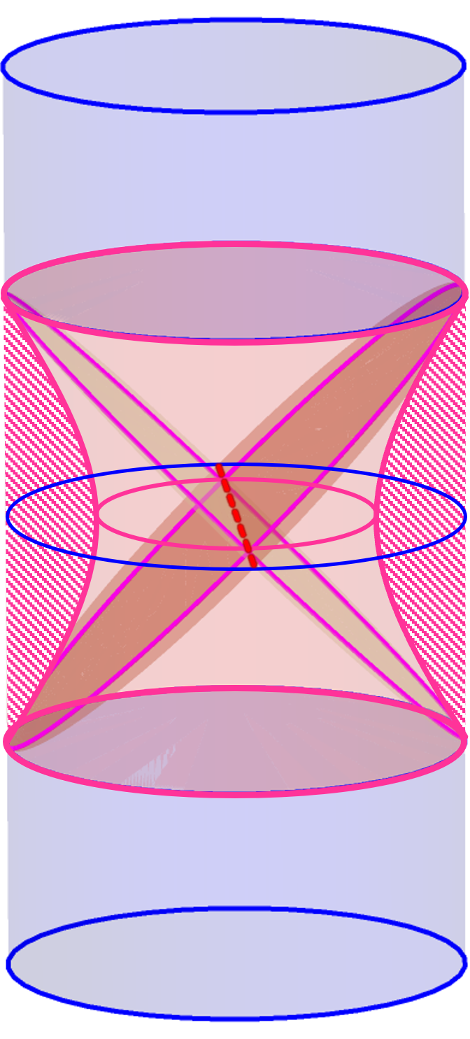
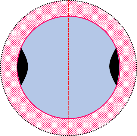
Figure 1: Left: Bulk $\text{AdS}_{4}$ with a de Sitter₃ brane. The brane is represented as a (magenta) hyperboloid. The bulk region up to the brane ($x<0$, dashed magenta region) is excluded. To complete the construction, we glue a second copy along the two-sided brane. Cosmological horizons on the dS brane corresponds to the bulk acceleration horizons intersecting the brane (red dashed line). Right: Constant $t$-time slice of a single $\text{AdS}_{4}$ cylinder with a de Sitter brane (thick red circle) containing black holes. The coordinates cover only half of the disk, containing only a single black hole and cosmological horizon, where the other half is obtained via an appropriate analytic continuation.

The geometry induced on the brane at $x=0$ will result in a metric in $(t,r,\phi)$-coordinates which has a conical deficit angle due to the identification (13). To respect regularity in the bulk, one thus rescales coordinates $(t,r,\phi)\to(\bar{t},\bar{r},\bar{\phi})$, where $t=\eta\bar{t}$, $r=\eta^{-1}\bar{r}$, and $\phi=\eta\bar{\phi}$, and $2\pi\eta\equiv\Delta\phi$, such that $\bar{\phi}$ is periodic in $2\pi$, and results in the geometry Emparan:2022ijy

$$ds^{2}_{\text{qSdS}}=-H(\bar{r})d\bar{t}^{2}+H^{-1}(\bar{r})d\bar{r}^{2}+\bar{r}^{2}d\bar{t}^{2}\;,\quad H(\bar{r})=1-8\mathcal{G}_{3}M-\frac{\ell F(M)}{\bar{r}}-\frac{\bar{r}^{2}}{R_{3}^{2}}\;.$$ (14)

This is the three-dimensional quantum Schwarzschild-de Sitter black hole. Depending on the size of $\ell F(M)$, there exist two positive roots to $H(\bar{r})=0$, denoted $\bar{r}_{+}$ and $\bar{r}_{c}$, the black hole and cosmological horizon, respectively. From the bulk perspective, the cosmological horizon on the brane arises due to the brane intersecting the acceleration horizon of the bulk black hole. Moreover, here the mass $M$ of the brane black hole and the form factor $F(M)$ are

$$8\mathcal{G}_{3}M\equiv 1-\frac{4x_{1}^{2}}{(3-x_{1}^{2})^{2}}\;,\quad F(M)\equiv\frac{8(1-x_{1}^{2})}{(3-x_{1}^{2})^{3}}\;,$$ (15)

with renormalized Newton’s constant $\mathcal{G}_{3}\equiv L_{4}G_{3}/\ell$. To arrive at the expression for $F(M)$, the parameter $\mu$ is treated as being “derived” from $G(x_{1})=0$, such that $x_{1}\in(0,1]$, where $x_{1}=1$ coincides with $\mu=0$ Emparan:2020znc .

We can think of the metric (14) as a semi-classical black hole because it is an exact solution to the holographically induced theory of gravity

$$I=\frac{1}{16\pi G_{3}}\int_{\mathcal{B}}d^{3}x\sqrt{-h}\left[R-\frac{2}{L_{3}^{2}}-L_{4}^{2}\left(R_{ij}^{2}-\frac{3}{8}R^{2}\right)+...\right]+I_{\text{CFT}}\;,$$ (16)

with semi-classical equations of motion

$$8\pi G_{3}\langle T^{\text{CFT}}_{ij}\rangle=G_{ij}+\frac{h_{ij}}{L_{3}^{2}}$$ (17)

$$+\ell^{2}\biggr{[}4R_{i}^{\;k}\tilde{R}_{jk}-\frac{9}{4}RR_{ij}-\Box R_{ij}+\frac{1}{4}\nabla_{i}\nabla_{j}R+\frac{1}{2}h_{ij}\left(\frac{13}{8}R^{2}-3R_{kl}^{2}+\frac{1}{2}\Box R\right)\biggr{]}+...\;.$$

The CFT stress-energy tensor sources the effective three-dimensional gravity theory such that backreaction is accounted for by $\langle T_{ij}^{\text{CFT}}\rangle$. Here we work in the limit where the effective three-dimensional theory obeys $L_{4}\ll L_{3}$, or, equivalently, $\ell\sim L_{4}$ such that $\ell/R_{3}$ is taken to be a small expansion parameter. Thus, the higher curvature terms in the action are multiplied by higher powers of $\ell$, where, from the brane perspective, $\ell$ captures the strength of backreaction. Hence, the higher-derivative corrections can be understood as a series of corrections due to semi-classical backreaction. In the limit of small backreaction, moreover, $L_{3}^{2}\approx R_{3}^{2}$ while the central charge $c\equiv L_{4}^{2}/G_{4}$ of the $\text{CFT}_{3}$ satisfies $2cG_{3}=L_{4}\approx\ell$. Therefore, for fixed $c$, gravity becomes weak on the brane as $\ell\to 0$ such that there is no backreaction due to the CFT. Lastly, $\ell\approx 2cL_{\text{P}}$, where $L_{\text{P}}=G_{3}$ is the Planck length (since we set $\hbar=1$).

Returning to the qSdS geometry (14), we see that the $\ell F(M)/\bar{r}$ contribution characterizes quantum-corrections to the classical $\text{SdS}_{3}$ solution. Since $\ell\approx 2cL_{\text{P}}$ and $c\gg 1$, as required by holography, the qSdS is not a Planck-sized black hole, but rather has a horizon much larger than the Planck length. Further, the renormalized Newton’s constant $\mathcal{G}_{3}$ (15) takes into account the modification of the definition of mass due to the higher curvature corrections Emparan:2020znc . Finally, we emphasize that analyzing the semi-classical Einstein’s equations for a free conformally coupled scalar results in the metric (14) to leading order in $L_{\text{P}}$ Emparan:2022ijy .

3 Geometry of quantum Kerr-$\text{dS}_{3}$ black holes

As reviewed above, braneworld holography grants us the ability to study the problem of semi-classical backreaction without having to explicitly solve semi-classical equations of motion. By a judicious choice of a bulk spacetime, the bulk black hole localizes on the brane and leads to the qSdS on the brane – the first known example of an exact quantum de Sitter black hole in the sense that the solution encodes all orders of semi-classical backreaction. Here we use braneworld holography to uncover the quantum Kerr-de Sitter black hole, focusing primarily on the geometry, leaving the thermodynamic analysis for the subsequent section.

3.1 Bulk and brane geometry

Analogous to the rotating quantum BTZ black hole Emparan:2020znc , our starting point is the rotating $\text{AdS}_{4}$ C-metric, describing accelerating Kerr-$\text{AdS}_{4}$ black holes and has the line element

$$\begin{split}ds^{2}&=\omega^{2}\biggr{(}-\frac{H(r)}{\Sigma}(dt-ax^{2}d\phi)^{2}+\frac{\Sigma}{H(r)}dr^{2}+r^{2}\left[\frac{\Sigma}{G(x)}dx^{2}+\frac{G(x)}{\Sigma}\left(d\phi+\frac{a}{r^{2}}dt\right)^{2}\right]\biggr{)}\end{split}$$ (18)

with metric functions

$$H(r)=1-\frac{r^{2}}{R_{3}^{2}}-\frac{\mu\ell}{r}+\frac{a^{2}}{r^{2}}\;,\quad G(x)=1-x^{2}-\mu x^{3}-\frac{a^{2}}{R_{3}^{2}}x^{4}\;,$$ (19)

$$\omega^{2}=\frac{\ell^{2}}{(\ell+xr)^{2}}\;,\quad\Sigma=1+\frac{a^{2}x^{2}}{r^{2}}\;.$$ (20)

Our conventions largely follow Emparan:2020znc , apart from the substitutions $R_{3}^{2}=-\ell_{3}^{2}$ (or $\ell_{3}=iR_{3}$) and $a\to-a$. Here $a$ is a parameter encoding the rotation of the bulk black hole (the angular momentum per unit mass), and in the limit $a=0$ we recover the static C-metric (9). Evaluating the bulk Kretschmann scalar invariant $\hat{R}^{abcd}\hat{R}_{abcd}$, there is a curvature singularity when $r^{2}\Sigma=r^{2}+a^{2}x^{2}=0$, i.e., when both $r=0$ and $x=0$. This is the familiar ring singularity in Kerr black holes.

Despite rotation, the $x=0$ hypersurface remains umbilic, obeying $K_{ij}=-\ell^{-1}h_{ij}$, and is thus a natural location to place the de Sitter brane. The geometry on the brane is

$$ds^{2}|_{x=0}=-H(r)dt^{2}+H^{-1}(r)dr^{2}+r^{2}\left(d\phi+\frac{a}{r^{2}}dt\right)^{2}\;.$$ (21)

Since the rotating C-metric (18) is a solution to the bulk Einstein equations, we are guaranteed the brane geometry is a solution to the induced theory of gravity (16). However, at this stage it would be naive to interpret this solution as the quantum Kerr-$\text{dS}_{3}$ black hole. This is because we have not yet accounted for bulk regularity conditions, which will affect more than just the periodicity of the angular variable $\phi$. In fact, we know the ‘naive metric’ (21) does not capture all of the correct features because the ring singularity lives on the brane, yet the above metric does not have a ring singularity at $r=0$ but rather a standard curvature singularity. We will see momentarily how the ring singularity makes an appearance.

Bulk regularity

Notice that the Killing vector $\partial_{\phi}$ no longer has vanishing norm at a zero $x_{i}$ of $G(x)$. Rather, the Killing vector

$$\xi^{b}=\partial^{b}_{\phi}+ax_{i}^{2}\partial^{b}_{t}\;,$$ (22)

obeys $\xi^{2}|_{x_{i}}=0$. Avoiding conical defects at $x=x_{i}$ requires us to identify points along the integral curves of the vector (22) with an appropriate period. To determine the correct periodicity, consider the rotating C-metric (18) near a zero $x=x_{i}$ such that $G(x)\sim G^{\prime}(x_{i})(x-x_{i})$ (see Appendix C). Removal of a conical singularity at $x=x_{i}$ requires one simultaneously perform the coordinate transformation $\tilde{t}=t-ax_{i}^{2}\phi$ together with the same periodicity condition on $\phi$ (13). Specifically, singling out the smallest positive root $x=x_{1}$, then

$$\phi\sim\phi+\Delta\phi\;,\quad\Delta\phi=\frac{4\pi}{|G^{\prime}(x_{1})|}=\frac{4\pi x_{1}}{3-x_{1}^{2}+\tilde{a}^{2}}\;,$$ (23)

where to arrive to the second equality we recast the parameter $\mu$ in terms of $x_{1}$

$$\mu=\frac{1-x_{1}^{2}-\tilde{a}^{2}}{x_{1}^{3}}\;,\quad\tilde{a}\equiv\frac{ax_{1}^{2}}{R_{3}}\;.$$ (24)

Thus, identifying points along the orbits of $\xi^{b}$ are made on surfaces of constant

$$\tilde{t}\equiv t-ax_{1}^{2}\phi\;.$$ (25)

The remaining zeros $x_{i}\neq x_{1}$ are dealt with by cutting off the bulk spacetime at $x=0$, and gluing to a second region such that the complete space is comprised of a bulk region with $x\in[0,x_{1}]$, leaving a space which is free of conical singularities at $x=x_{i}$.

Returning to the naive geometry at $x=0$ (21), consider the asymptotic limit $r\to\infty$. The metric is asymptotic to ‘rotating $\text{dS}_{3}$’, where the $dtd\phi$ component grows like a constant. Unfortunately, the coordinates are not canonically normalized due to the periodicity in $\phi$ (23). In fact, since points along orbits of (22) are identified, the periodicity in $\phi$ (23) returns one to a different point in time $t$: from (25), we see that with $\tilde{t}\sim\tilde{t}$ then $t\sim t+2\pi\eta ax_{1}^{2}$, where $\eta\equiv\Delta\phi/2\pi$. This means we cannot just rescale coordinates $(t,r,\phi)\to(\bar{t},\bar{r},\bar{\phi})$ as done in the static case (14). Additionally, the periodicity alters the asymptotic form of the metric such that the $dtd\phi$ grows as $r^{2}$, which would seem to imply a diverging angular momentum.

We can remedy the situation by changing coordinates $(t,\phi)$ to $(\tilde{t},\tilde{\phi})$ where $t=\tilde{t}+ax_{1}^{2}\tilde{\phi}$ and $\phi=\tilde{\phi}+C\tilde{t}$ for some constant $C$. In the asymptotic limit, the $\tilde{t}-\tilde{\phi}$ component of the naive brane metric (21) will have go as

$$h_{\tilde{t}\tilde{\phi}}=\left(C+\frac{ax_{1}^{2}}{R_{3}^{2}}\right)r^{2}+(a-ax_{1}^{2}+Ca^{2}x_{1}^{2})+\mathcal{O}(1/r)\;.$$ (26)

Judiciously, we choose $C\equiv-ax_{1}^{2}/R_{3}^{2}=-\tilde{a}/R_{3}$ to eliminate the $r^{2}$ divergence. Making this choice deals with the undesired asymptotic growth, however, $\tilde{\phi}$ is still not periodic in $2\pi$. This is now easily resolved by a simple rescaling, $\tilde{t}=\eta\bar{t}$ and $\tilde{\phi}=\eta\bar{\phi}$, such that the transformation

$$t=\eta(\bar{t}+\tilde{a}R_{3}\bar{\phi})\;,\quad\phi=\eta\left(\bar{\phi}-\frac{\tilde{a}}{R_{3}}\bar{t}\right)\;,$$ (27)

puts the brane geometry in a more canonical form. Inverting the transformation (27),

$$\bar{t}=\frac{1}{\eta(1+\tilde{a}^{2})}(t-\tilde{a}R_{3}\phi)\;,\quad\bar{\phi}=\frac{1}{\eta(1+\tilde{a}^{2})}\left(\phi+\frac{\tilde{a}}{R_{3}}t\right)\;,$$ (28)

we see the Killing vectors $\partial_{t}$ and $\partial_{\phi}$ transform as

$$\partial_{t}=\frac{1}{\eta(1+\tilde{a}^{2})}\left(\partial_{\bar{t}}+\frac{\tilde{a}}{R_{3}}\partial_{\bar{\phi}}\right)\;,\quad\partial_{\phi}=\frac{1}{\eta(1+\tilde{a}^{2})}\left(\partial_{\bar{\phi}}-\tilde{a}R_{3}\partial_{\bar{t}}\right)\;.$$ (29)

Consequently, now the rotational Killing vector (22) is $\xi^{b}=\eta^{-1}\partial_{\bar{\phi}}$.

With the coordinate change (27), the brane metric does not quite have the canonical asymptotic form of a rotating de Sitter black hole. We still need to redefine the radial coordinate $r$. Following Emparan:2020znc , let

$$r^{2}\equiv\frac{\bar{r}^{2}-r_{s}^{2}}{(1+\tilde{a}^{2})\eta^{2}}\;,\quad r_{s}=-\frac{R_{3}\tilde{a}\eta}{x_{1}}\sqrt{2-x_{1}^{2}}=-\frac{2\tilde{a}R_{3}\sqrt{2-x_{1}^{2}}}{3-x_{1}^{2}+\tilde{a}^{2}}\;.$$ (30)

Altogether, the geometry on the brane in the canonically normalized coordinates $(\bar{t},\bar{r},\bar{\phi})$ is

$$\begin{split}ds^{2}|_{x=0}&=-\left(\eta^{2}\left(1-\tilde{a}^{2}+\frac{4\tilde{a}^{2}}{x_{1}^{2}}\right)-\frac{\bar{r}^{2}}{R_{3}^{2}}-\frac{\mu\ell\eta^{2}}{r}\right)d\bar{t}^{2}\\ &+\left(\eta^{2}\left(1-\tilde{a}^{2}+\frac{4\tilde{a}^{2}}{x_{1}^{2}}\right)-\frac{\bar{r}^{2}}{R_{3}^{2}}-\frac{\mu\ell(1+\tilde{a}^{2})^{2}\eta^{4}r}{\bar{r}^{2}}+\frac{R_{3}^{2}\tilde{a}^{2}\mu^{2}x_{1}^{2}\eta^{4}}{\bar{r}^{2}}\right)^{-1}d\bar{r}^{2}\\ &+\left(\bar{r}^{2}+\frac{\mu\ell\tilde{a}^{2}R_{3}^{2}\eta^{2}}{r}\right)d\bar{\phi}^{2}+R_{3}\tilde{a}\mu x_{1}\eta^{2}\left(1+\frac{\ell}{x_{1}r}\right)(d\bar{\phi}d\bar{t}+d\bar{t}d\bar{\phi})\;,\end{split}$$ (31)

where we have kept both $r$ and $\bar{r}$ when convenient.

3.2 Black hole on the brane

Let us now scrutinize the brane geometry (31). First, we identify the mass $M$ as

$$8\mathcal{G}_{3}M\equiv 1-\eta^{2}\left(1-\tilde{a}^{2}+\frac{4\tilde{a}^{2}}{x_{1}^{2}}\right)=1-\frac{4[x_{1}^{2}-\tilde{a}^{2}(x_{1}^{2}-4)]}{(3-x_{1}^{2}+\tilde{a}^{2})^{2}}\;,$$ (32)

where $\mathcal{G}_{3}\equiv L_{4}G_{3}/\ell$ is the ‘renormalized’ three-dimensional Newton’s constant Emparan:2020znc . Since the brane theory is generally three-dimensional Einstein-de Sitter gravity plus higher-derivative corrections, we do not have a generic Komar-like mass integral in which we compute $M$. Rather, here we have identified the mass as the subleading constant term in $h_{\bar{t}\bar{t}}$, as done in Einstein-de Sitter gravity, and used $\mathcal{G}_{3}$ to encompass all of the higher-derivative corrections entering at order $\ell^{2}$ in the brane action (16) Cremonini:2009ih . Similarly, we have identified the three-dimensional angular momentum $J$ to be

$$4\mathcal{G}_{3}J\equiv-R_{3}\tilde{a}\mu x_{1}\eta^{2}=\frac{4R_{3}\tilde{a}(x_{1}^{2}+\tilde{a}^{2}-1)}{(3-x_{1}^{2}+\tilde{a}^{2})^{2}}\;,$$ (33)

where again the renormalized Newton’s constant plays the role of accounting for higher-derivative corrections to the angular momentum. Importantly, notice $M$ and $J$ depend on $\tilde{a}^{2}$ and $x_{1}^{2}$, and the parameter $\ell$ does not make an explicit appearance.

We emphasize, at this stage, the mass $M$ (32) and angular momentum $J$ (33) are identifications. Justification for this, in part, comes from the fact that these quantities satisfy a first law of thermodynamics, as we demonstrate in the next section. Essentially, as argued in Emparan:2002px the mass of the black hole on the brane is identified as the mass of the bulk black hole intersecting the brane. A feature distinguishing AdS and dS braneworld constructions is how the mass (32) coincides with a conserved charge. This is because asymptotically dS spacetimes do not have a boundary which makes providing an invariant notion of conserved charges more difficult. From the brane perspective, one could compute conserved charges, for example, by calculating the Brown-York quasi-local stress tensor on slices at past and future infinity Balasubramanian:2001nb . The mass found should then coincide with the mass of the bulk black hole intersecting the brane at $I^{\pm}$. In practice this is difficult, however, because the theory on the brane is a complicated higher-order theory of gravity, a context in which defining conserved charges is also a subtle matter (AdS braneworld models encounter the same subtlety in this regard). Alternatively, one can use the method developed in Dolan:2018hpl , which does not require entering an asymptotic region. It would be worthwhile to explore this question and verify the mass identified in the first law coincides with an invariant conserved charge.

With the substitutions (32) and $J$ (33)s, the brane geometry (31) takes the form

$$\begin{split}ds^{2}_{\text{qKdS}}&=-\left(1-8\mathcal{G}_{3}M-\frac{\bar{r}^{2}}{R_{3}^{2}}-\frac{\mu\ell\eta^{2}}{r}\right)d\bar{t}^{2}\\ &+\left(1-8\mathcal{G}_{3}M-\frac{\bar{r}^{2}}{R_{3}^{2}}+\frac{(4\mathcal{G}_{3}J)^{2}}{\bar{r}^{2}}-\frac{\mu\ell(1+\tilde{a}^{2})^{2}\eta^{4}r}{\bar{r}^{2}}\right)^{-1}d\bar{r}^{2}\\ &+\left(\bar{r}^{2}+\frac{\mu\ell\tilde{a}^{2}R_{3}^{2}\eta^{2}}{r}\right)d\bar{\phi}^{2}-4\mathcal{G}_{3}J\left(1+\frac{\ell}{x_{1}r}\right)(d\bar{\phi}d\bar{t}+d\bar{t}d\bar{\phi})\;.\end{split}$$ (34)

Since the metric (34) is an exact solution to the full semi-classical theory of gravity on the brane (17), we refer to the three-dimensional spacetime as the quantum Kerr-$\text{dS}_{3}$ black hole (qKdS). We say ‘black hole’ because, as we describe below, this geometry possesses both an inner and outer black hole horizon, shrouding a ring singularity, and a cosmological horizon. We say ‘quantum’ because it includes all orders of semi-classical backreaction due to the CFT, where terms in the metric proportional to $\mu\ell$ are understood to be quantum corrections to the classical Kerr-$\text{dS}_{3}$ conical defect. Justification of this terminology will be given when we compute the renormalized CFT stress-tensor $\langle T^{\text{CFT}}_{ij}\rangle$.

Before we analyze the brane geometry (34) in more detail, there are a few special limits to consider. First, clearly, when the rotation $a\to 0$, then $J=0$ and the geometry reduces to the static metric (14), the quantum Schwarzschild-de Sitter black hole Emparan:2022ijy . Next, in the limit of vanishing backreaction $\ell\to 0$, in which the gravitational effects of the cutoff CFT are suppressed (where $\mathcal{G}_{3}\to G_{3}$), the metric (34) takes the form of the classical Kerr-$\text{dS}_{3}$ conical defect spacetime (see Appendix A). Thirdly, when the parameter $\mu$ (24) vanishes, i.e., $x_{1}=\sqrt{1-\tilde{a}^{2}}$, then both $M=J=0$, resulting in the empty $\text{dS}_{3}$ geometry. The mass $M$ will also be zero when $x_{1}=\sqrt{9-\tilde{a}^{2}}$. When this is the case, $J\neq 0$ and $\mu\neq 0$,

$$4\mathcal{G}_{3}J=\frac{32\tilde{a}R_{3}}{(6-2\tilde{a}^{2})^{2}}\;,\quad\mu=\frac{512\tilde{a}R_{3}}{(\tilde{a}^{2}-9)^{3}(\tilde{a}^{2}-3)^{2}}\;,$$ (35)

and we can think of the brane geometry as quantum rotating $\text{dS}_{3}$.

Horizons and closed timelike curves

While the metric (34) is in the correct canonically normalized coordinates $(\bar{t},\bar{r},\bar{\phi})$, in what follows we will perform calculations in the naive background $(t,r,\phi)$ (21), and perform the appropriate coordinate transformation. This is largely done for convenience, but also because both metrics share nearly all of the same qualitative features.

In the static case, roots of $H(r)$ correspond to the Killing horizons of the Killing vector $\partial_{t}$. With rotation, the Killing vector

$$\zeta^{b}=\partial_{t}-\frac{a}{r_{i}^{2}}\partial_{\phi}\;$$ (36)

becomes null at roots $r_{i}$ of $H(r)$. Define the function $Q(r)\equiv r^{2}H(r)$. Since $Q(r)$ is a quartic polynomial in $r$, it will generally have either four, two, or zero real roots. Here we focus on the case when there are four real roots, which we will see later enforces conditions on the physical parameters $a$ and $\mu$. The three positive roots to $Q(r)$ are the cosmological horizon $r_{c}$, the outer black hole horizon $r_{+}$ and inner black hole horizon $r_{-}$, obeying $r_{-}\leq r_{+}\leq r_{c}$. The fourth root, $r_{n}$, is negative and resides behind the singularity at $r=0$. Using $H(r_{c})=0$, and $H(r_{\pm})=0$, we can express

$$\begin{split}&R_{3}^{2}=r_{c}^{2}+r_{+}^{2}+r_{c}r_{+}+r_{-}(r_{c}+r_{+}+r_{-})\;,\\ &\mu\ell=\frac{(r_{c}+r_{+})(r_{c}+r_{-})(r_{+}+r_{-})}{r_{c}^{2}+r_{+}^{2}+r_{c}r_{+}+r_{-}(r_{c}+r_{+}+r_{-})}\;,\\ &a^{2}=\frac{r_{c}r_{+}r_{-}(r_{c}+r_{+}+r_{-})}{r_{c}^{2}+r_{+}^{2}+r_{c}r_{+}+r_{-}(r_{c}+r_{+}+r_{-})}\;.\end{split}$$ (37)

The blackening factor $H(r)$ factorizes as

$$\begin{split}H(r)&=\frac{1}{R_{3}^{2}r^{2}}(r_{c}-r)(r-r_{+})(r-r_{-})(r+r_{c}+r_{+}+r_{-})\;.\end{split}$$ (38)

The limit $r_{-}\to 0$ coincides with $a=0$, while $r_{+}=r_{-}=0$ corresponds to $\mu\to 0$, resulting in the Kerr-$\text{dS}_{3}$ geometry with a single cosmological horizon.

Since the black hole is stationary, the positive roots $r_{i}$ to $H(r)$ correspond to rotating horizons with rotation $\Omega_{i}$,

$$\Omega_{i}\equiv\frac{a}{R_{3}^{2}}\frac{(x_{1}^{2}r_{i}^{2}-R_{3}^{2})}{(r_{i}^{2}+a^{2}x_{1}^{2})}\;,$$ (39)

where we used the transformations (29), to express $\zeta^{b}$ and define $\bar{\zeta}^{b}$

$$\bar{\zeta}^{b}\equiv\frac{\eta(1+\tilde{a}^{2})}{\left(1+\frac{a^{2}x_{1}^{2}}{r_{i}^{2}}\right)}\zeta^{b}=\partial_{\bar{t}}^{b}+\Omega_{i}\partial_{\bar{\phi}}^{b}\;.$$ (40)

Further, relative to $\bar{\zeta}^{b}$, the surface gravity $\kappa_{i}$ associated with each horizon $r_{i}$ is given by

$$\kappa_{i}=\frac{\eta(1+\tilde{a}^{2})}{\left(r_{i}^{2}+a^{2}x_{1}^{2}\right)}\frac{r_{i}^{2}}{2}|H^{\prime}(r_{i})|=\frac{\eta(1+\tilde{a}^{2})}{\left(r_{i}^{2}+a^{2}x_{1}^{2}\right)}\frac{1}{2R_{3}^{2}r_{i}}|R_{3}^{2}\mu\ell r_{i}-2r_{i}^{4}-2a^{2}R_{3}^{2}|\;,$$ (41)

where we used the definition $\bar{\zeta}^{b}\nabla_{b}\bar{\zeta}^{c}=\kappa\bar{\zeta}^{c}$. Explicitly,

$$\begin{split}&\kappa_{c}=-\frac{\eta(1+\tilde{a}^{2})}{2R_{3}^{2}\left(r_{c}^{2}+a^{2}x_{1}^{2}\right)}(r_{c}-r_{+})(r_{c}-r_{-})(r_{+}+r_{-}+2r_{c})\;,\\ &\kappa_{+}=\frac{\eta(1+\tilde{a}^{2})}{2R_{3}^{2}\left(r_{+}^{2}+a^{2}x_{1}^{2}\right)}(r_{c}-r_{+})(r_{+}-r_{-})(r_{c}+r_{-}+2r_{+})\;,\\ &\kappa_{-}=-\frac{\eta(1+\tilde{a}^{2})}{2R_{3}^{2}\left(r_{-}^{2}+a^{2}x_{1}^{2}\right)}(r_{c}-r_{-})(r_{+}-r_{-})(r_{c}+r_{+}+2r_{-})\;.\end{split}$$ (42)

Notice the cosmological horizon surface gravity $\kappa_{c}$ vanishes when $r_{c}=r_{+}$ or $r_{c}=r_{-}$, and similarly for the other surface gravities. We explore these extremal limits momentarily. When $r_{-}\to 0$, i.e., vanishing rotation, we recover the surface gravities of the cosmological horizon and black hole horizon of the qSdS black hole Emparan:2022ijy . Additionally, in the limit of vanishing backreaction, then $r_{\pm}\to 0$ such that $\kappa_{\pm}\to 0$.

As mentioned previously, in the naive coordinates (21), a computation of the Kretschmann scalar reveals a curvature singularity at $r=0$. In the canonically normalized coordinates (34), $r=0$ corresponds $\bar{r}=r_{s}$, corresponding to a ring singularity, and is endowed from the bulk black hole solution. Moreover, near the ring singularity there exists the possibility of closed timelike curves. Relative to the canonically normalized metric (34), the norm of the axial Killing vector $\partial_{\bar{\phi}}$ is

$$\partial_{\bar{\phi}}^{2}=h_{\bar{\phi}{\phi}}=\bar{r}^{2}+\frac{\mu\ell\tilde{a}^{2}R_{3}^{2}\eta^{2}}{r}\;.$$ (43)

Thus, for sufficiently small and negative $r$, the vector $\partial_{\bar{\phi}}$ becomes timelike, the orbits of which are closed curves around the rotation axis. However, unlike the rotating qBTZ black hole, these closed timelike curves do not become naked.

When all of the roots to $Q(r)$ are distinct, then standard methods Gibbons:1977mu lead to a maximal extension of the quantum Kerr-$\text{dS}_{3}$ black hole. Generally, the resulting conformal diagram is infinite in extent and is nearly identical to the Kruskal extension of the classical four-dimensional Kerr-dS black hole. The aforementioned closed timelike curves may be eliminated by an appropriate periodic identification Booth:1998gf , such that constant $\bar{t}$ hypersurfaces are closed and span two black hole regions with opposite spin, cutting through intersections of $r=r_{c}$ and $r=r_{+}$ (see Figure 2 for a diagram).

Figure 2: Penrose diagram of a neutral quantum Kerr black hole in dS₃. Shown here is the global structure with periodic identifications made along constant $\bar{t}$ hypersurfaces. The diagram has infinite extent in the vertical directions while the dashed edges are identified.

Ergoregions

As with classical Kerr-de Sitter spacetimes, the qKdS black hole has a stationary limit surface and two ergoregions associated with the outer black hole and cosmological horizons. Explicitly, the time-translation Killing vector $\partial_{t}$ in the naive metric has the norm $\mathcal{N}$

$$\mathcal{N}=-H(r)+\frac{a^{2}}{r^{2}}\;.$$ (44)

Clearly, at the outer and cosmological horizons, where $H=0$, then $\partial_{t}$ is spacelike. The locus of points where $\mathcal{N}=0$ yields a stationary limit surface, satisfying $r(R_{3}^{2}-r^{2})=R_{3}^{2}\mu\ell$. Since there exist regions in between the outer and cosmological horizons where $\partial_{t}$ is timelike, there are two ergoregions, where an observer is forced to move in the direction of rotation of the outer black hole horizon or cosmological horizon (the black hole and cosmological ergoregions, respectively). With the appearance of ergoregions, one can in principle examine the Penrose process of energy extraction in the qKdS solution in morally the same way as a classical four-dimensional Kerr-de Sitter black hole (see, e.g., Bhattacharya:2017scw ). At least for small backreaction, it is expected the Penrose process in the cosmological ergoregion is not possible.

3.3 Extremal, Nariai, ultracold, and lukewarm limits

As with the four-dimensional Kerr-de Sitter black hole, the quantum Kerr-$\text{dS}_{3}$ has a number of limiting geometries. Specifically, (i) extremal or ‘cold’ limit, where $r_{+}=r_{-}$; (ii) rotating Nariai limit, where $r_{c}=r_{+}$; (iii) the ‘ultacold’ limit where $r_{c}=r_{+}=r_{-}$, and (iv) the ‘lukewarm’ limit, where the surface gravities $\kappa_{c}=\kappa_{+}$. Below we summarize each of these limiting geometries and briefly explore their features, leaving the details to Appendix D. Our analysis primarily follows Booth:1998gf , and for simplicity, we work with the naive metric $(t,r,\phi)$ (21) except when stated otherwise.

Extremal black hole: $r_{+}=r_{-}$

The extremal black hole corresponds to when the outer and inner black hole horizons coincide. In this limit the surface gravity of the outer horizon $\kappa_{+}=0$, and, correspondingly the Hawking temperature $T_{+}$ of the black hole vanishes, i.e., the black hole is ‘cold’. Moreover, parameters $a^{2}$ and $\mu\ell$ may be cast as

$$a^{2}=r_{+}^{2}-\frac{3r_{+}^{4}}{R_{3}^{2}}\;,\quad\mu\ell=2r_{+}-\frac{4r_{+}^{3}}{R_{3}^{2}}\;.$$ (45)

In the extremal limit the global structure of the spacetime changes because now the (double) black hole horizon moves to an infinite proper distance away from all other portions of the geometry, such that the black hole interior is inaccessible from the rest of the spacetime.

In the near horizon limit of extremal qKdS, we can no longer express the metric in coordinates $(t,r,\phi)$ as they become singular. Rather, we perform a coordinate transformation analogous to Bardeen:1999px ; Hartman:2008pb

$$r=r_{+}+\lambda\rho\;,\quad t=\frac{\tau}{\lambda}\;,\quad\phi=\varphi-\frac{a\tau}{r_{+}^{2}\lambda}\;,$$ (46)

where upon taking $\lambda\to 0$ we find

$$ds^{2}_{\text{ex}}=\Gamma\left(-\hat{\rho}^{2}d\hat{\tau}^{2}+\frac{d\hat{\rho}^{2}}{\hat{\rho}^{2}}\right)+r_{+}^{2}\left(d\varphi+k\hat{\rho}d\hat{\tau}\right)^{2}\;,$$ (47)

with

$$\Gamma=\frac{r_{+}^{2}}{1-6r_{+}^{2}/R_{3}^{2}}\;,\quad k=-\frac{2aR_{3}^{2}}{r_{+}(R_{3}^{2}-6r_{+}^{2})}\;.$$ (48)

This is the near horizon extremal Kerr (NHEK) geometry for the quantum-corrected Kerr-$\text{dS}_{3}$. Formally it has the same structure as the NHEK region of four-dimensional Kerr-(A)dS spacetimes, and has the form of a fibered product of $\text{AdS}_{2}$ and the circle. As such, following Hartman:2008pb , the isometry group is $\text{SL}(2,\mathbb{R})\times U(1)$.

Notice from (45) that $a=0$ when $r_{+}=0$ or $r_{+}=R_{3}/\sqrt{3}$, which, respectively, corresponds to $\mu\ell=0$ or $\mu\ell=2R_{3}/3\sqrt{3}$. The latter is simply the Nariai limit of the quantum Schwarzschild-de Sitter black hole Emparan:2022ijy , which we explore in more detail below.

Rotating Nariai black hole: $r_{c}=r_{+}$

The Nariai solution occurs when the cosmological and outer black hole horizons coincide $r_{c}=r_{+}\equiv r_{\text{N}}$. Then

$$a^{2}=\frac{r_{\text{N}}^{2}}{R_{3}^{2}}(R_{3}^{2}-3r_{\text{N}}^{2})\;,\quad(\mu\ell)_{\text{N}}=\frac{2r_{\text{N}}}{R_{3}^{2}}(R_{3}^{2}-2r_{\text{N}}^{2})\;.$$ (49)

Notice when $a=0$ we recover $r_{\text{N}}=R_{3}/\sqrt{3}$ and $(\mu\ell)_{\text{N}}=2R_{3}/3\sqrt{3}$, the Nariai limit of the static Schwarzschild-de Sitter black hole. Physically, the Nariai black hole is the largest black hole which may fit inside the cosmological horizon, saturating at $\mu_{\text{N}}$. Moreover, the rotating Nariai black hole is generally larger than the static Nariai solution, analogous to how the charged Nariai black hole is larger than the neutral geometry.

The blackening factor $H(r)$ vanishes when $r=r_{\text{N}}$ making the $(t,r,\phi)$ coordinate system incompatible in describing the Nariai geometry. Thus, introduce coordinates Booth:1998gf

$$r=r_{\text{N}}+\epsilon\rho\;,\quad t=\frac{\Gamma\hat{\tau}}{\epsilon}\;,\quad\phi=\varphi-\frac{a}{r_{\text{N}}^{2}\epsilon}\tau\;.$$ (50)

and send $\epsilon\to 0$ such that the naive geometry (21) becomes

$$ds^{2}_{\text{N}}=\Gamma\left(-(1-\rho^{2})d\hat{\tau}^{2}+\frac{d\rho^{2}}{(1-\rho^{2})}\right)+r_{\text{N}}^{2}\left(d\varphi+k\rho d\hat{\tau}\right)^{2}\;,$$ (51)

where

$$\Gamma=\frac{R_{3}^{2}r_{\text{N}}^{2}}{6r_{\text{N}}^{2}-R_{3}^{2}}\;,\quad k=-\frac{2aR_{3}^{2}}{r_{\text{N}}(6r_{\text{N}}^{2}-R_{3}^{2})}\;.$$ (52)

Hence, the Nariai limit of the qKdS black hole has the product structure of $\text{dS}_{2}$ fibered over a circle, written here in static patch coordinates, and has the isometry group $U(1)\times\text{SL}(2,\mathbb{R})$. When $a=0$, then $\Gamma=R_{3}^{2}/3$, leading to the non-rotating Nariai metric Nariai99 ; Ginsparg:1982rs ; Cardoso:2004uz with product geometry $\text{dS}_{2}\times S_{2}$. A static patch observer is restricted to the region $\rho\in(-1,1)$, where $\rho=-1$ corresponds to the black hole horizon and $\rho=+1$ the cosmological horizon, at a finite proper distance apart. To draw the Penrose diagram (see Figure 3) it is useful to switch to global coordinates Anninos:2009yc

Figure 3: Penrose diagram of the Nariai qKdS black hole. The black hole and cosmological horizons are located at $\rho=-1$ and $\rho=1$, respectively, and are in thermal equilibrium at a non-zero temperature. Clearly there is a finite proper distance between the two horizons. Future and past infinity $\mathcal{I}^{\pm}$ are located at $\rho=\infty$, while the past and future black hole singularities correspond to $\rho=-\infty$. The left and right sides of the diagram are identified.

$$\begin{split}&\tan(\eta/2)=\tanh\left(\frac{1}{2}\sinh^{-1}(\sqrt{1-\rho^{2}}\sinh\hat{\tau})\right)\\ &\cos\psi=\rho(\cosh^{2}\hat{\tau}-\rho^{2}\sinh^{2}\hat{\tau})^{-1/2}\\ &\chi=\varphi+\frac{k}{2}\log\left(\frac{\sin(\eta+\psi)}{\sin(\eta-\psi)}\right)\;,\end{split}$$ (53)

such that

$$ds^{2}_{\text{N}}=\Gamma\left(\frac{-d\eta^{2}+d\psi^{2}}{\cos^{2}\eta}\right)+r_{\text{N}}^{2}(d\chi+k\tan\eta d\psi)^{2}\;,$$ (54)

where $\psi\sim\psi+2\pi$ and $\eta\in(-\pi/2,\pi/2)$ cover the all of the $\text{dS}_{2}$ portion.

Naively, when $r_{c}=r_{+}$ the surface gravities (41) of the cosmological and black hole horizons vanish, $\kappa_{c}=\kappa_{+}=0$. However, in the Nariai geometry (51), the two horizons are in thermal equilibrium at a non-zero temperature $T_{\text{N}}$. We will return to this in Section 4.

Ultracold black hole: $r_{c}=r_{+}=r_{-}$

The ultracold black hole is the limit when all of the horizons coincide, namely, $r_{c}=r_{+}=r_{-}\equiv r_{uc}$. The form of the metric can be found directly from the Nariai geometry (51). Since the Nariai geometry becomes singular when $r_{\text{N}}=r_{-}$, the coordinates $(\rho,\hat{\tau})$ require an appropriate rescaling

$$\rho=\sqrt{\frac{2r_{\text{uc}}-\delta}{R_{3}}}X\;,\quad\tau=\sqrt{\frac{R_{3}}{2r_{\text{uc}}-\delta}}\frac{R_{3}r_{\text{uc}}}{4}T\;,$$ (55)

where $\tau=\Gamma\hat{\tau}$, and subsequently take the limit $\delta\to 2r_{\text{uc}}$. The resulting geometry is

$$ds^{2}_{\text{uc}}=\frac{R_{3}r_{\text{uc}}}{4}(-dT^{2}+dX^{2})+r_{\text{uc}}^{2}\left(d\varphi-\frac{2aX}{r_{\text{uc}}^{3}}dT\right)^{2}\;.$$ (56)

This geometry is of the form of a fibered product of two-dimensional Minkowski space over a circle. Via an appropriate coordinate transformation (see Booth:1998gf ), the ultracold solution can also be expressed as a fibered product of two-dimensional Rindler space and a circle. In the limit of vanishing rotation there is no ultracold solution, but rather a static Nariai black hole.

Lukewarm black hole: $\kappa_{c}=\kappa_{+}$

As with all Kerr-de Sitter black holes, the quantum Kerr-$\text{dS}_{3}$ has a lukewarm limit. This occurs when the surface gravities of the cosmological and outer black hole horizons coincide at a value different from the surface gravity of the Nariai black hole. Notably, the geometry is non-singular in $(t,r,\phi)$ coordinates. Thermodynamically speaking, this spacetime is another example of where the black hole and cosmological horizon are in thermal equilibrium. We will return to this limit in Section 4, however, in Appendix D we find its limiting form in the naive brane geometry.

Before moving on, we point out that the special limits of the quantum Kerr-$\text{dS}_{3}$ black hole has qualitatively similar features to $\text{dS}_{3}$ black hole solutions to topologically massive gravity, cf. Nutku:1993eb ; Anninos:2009jt ; Anninos:2011vd . Indeed, the asymptotically warped $\text{dS}_{3}$ black hole (obtained from discrete global identifications of warped $\text{dS}_{3}$) has a Nariai limit whose $U(1)\times U(1)$ isometry is enhanced to a $\text{SL}(2,\mathbb{R})\times U(1)$ isometry group. It would be interesting to understand the relation between quantum $\text{dS}_{3}$ black holes and warped $\text{dS}_{3}$ black holes in more detail.

3.4 Holographic conformal matter stress-tensor

We have been referring to the geometry on the brane (34) as a quantum black hole since, via the holographic dictionary, it is a solution to the semi-classical equations of motion (17) to all orders in backreaction. Let us now justify this claim and solve for the expectation value of the CFT stress-energy tensor $\langle T_{ij}\rangle$ sourcing the black hole.

Following Emparan:2020znc , we decompose $\langle T^{i}_{\;j}\rangle=\langle T^{i}_{\;j}\rangle_{0}+\ell^{2}\langle T^{i}_{\;j}\rangle_{2}+...$ in increasing powers of $\ell^{2}$. Specifically, the leading order contribution is

$$8\pi G_{3}\langle T^{i}_{\;j}\rangle_{0}=R^{i}_{\;j}-\frac{1}{2}\delta^{i}_{\;j}\left(R-\frac{2}{R_{3}^{2}}\right)\;,$$ (57)

while the $\mathcal{O}(\ell^{2})$ contribution is

$$\begin{split}8\pi G_{3}\langle T^{i}_{\;j}\rangle_{2}&=4R^{ik}R_{jk}-\Box R^{i}_{\;j}-\frac{9}{4}RR^{i}_{\;j}+\frac{1}{4}\nabla^{i}\nabla_{j}R\\ &+\frac{1}{2}\delta^{i}_{\;j}\left(\frac{13}{8}R^{2}-3R_{kl}^{2}+\frac{1}{2}\Box R-\frac{1}{2R_{3}^{4}}\right)\;.\end{split}$$ (58)

It proves is more computationally convenient to determine $\langle T_{ij}\rangle$ in the naive metric (21) and then transform into the $(\bar{t},\bar{r},\bar{\phi})$ than working directly with the metric (34). Thus, in the naive background we find the only non-vanishing components of the stress-tensor are

$$\begin{split}&\langle T^{t}_{\;t}\rangle_{0}=\langle T^{r}_{\;r}\rangle_{0}=-\frac{1}{2}\langle T^{\phi}_{\;\phi}\rangle_{0}=\frac{1}{16\pi G_{3}}\frac{\mu\ell}{r^{3}}\;,\\ &\langle T^{\phi}_{\;t}\rangle_{0}=-\frac{1}{16\pi G_{3}}\frac{3\mu\ell a}{r^{5}}\;,\end{split}$$ (59)

and, for completeness,

$$\begin{split}&\langle T^{t}_{\;t}\rangle_{2}=-\frac{\mu\ell}{32\pi G_{3}R_{3}^{2}r^{7}}\left[90a^{2}R_{3}^{2}-11r^{4}+R_{3}^{2}r(18r-19\mu\ell)\right]\;,\\ &\langle T^{r}_{\;r}\rangle_{2}=-\frac{\mu\ell}{32\pi G_{3}R_{3}^{2}r^{7}}\left[r^{4}+30a^{2}R_{3}^{2}+R_{3}^{2}r(6r-7\mu\ell)\right]\;,\\ &\langle T^{\phi}_{\;\phi}\rangle_{2}=-\frac{\mu\ell}{32\pi G_{3}R_{3}^{2}r^{7}}\left[10r^{4}-120a^{2}R_{3}^{2}-R_{3}^{2}r(24r-29\mu\ell)\right]\;,\\ &\langle T^{t}_{\;\phi}\rangle_{2}=-\frac{3a\mu\ell}{2\pi G_{3}r^{5}}\;,\\ &\langle T^{\phi}_{\;t}\rangle_{2}=-\frac{3a\mu\ell}{32\pi G_{3}R_{3}^{2}r^{9}}\left[23r^{4}-70a^{2}R_{3}^{2}-R_{3}^{2}r(30r-32\mu\ell)\right]\;\end{split}$$ (60)

Notice that while $\langle T^{i}_{\;i}\rangle_{0}=0$, as one would expect for a CFT stress-tensor, we see $\langle T^{i}_{i}\rangle_{2}=-3(\mu\ell)^{2}/32\pi G_{3}r^{6}$. A non-termminating trace at higher order powers is a consequence of the fact that the CFT on the brane has an ultraviolet cutoff.

Transforming to the $(\bar{t},\bar{r},\bar{\phi})$ coordinates

$$\langle T^{\bar{i}}_{\;\bar{j}}\rangle=\Lambda^{\bar{i}}_{\;i}\Lambda^{j}_{\;\bar{j}}\langle T^{i}_{\;j}\rangle\;,\quad\Lambda^{\bar{i}}_{\;j}\equiv\frac{\partial\bar{x}^{i}}{\partial x^{j}}=\frac{1}{\eta(1+\tilde{a}^{2})}\begin{pmatrix}1&0&-\tilde{a}R_{3}\\ 0&r\sqrt{\frac{1+\tilde{a}^{2}}{r^{2}-r_{s}^{2}}}&0\\ -\frac{\tilde{a}}{R_{3}}&0&1\end{pmatrix}\;,$$ (61)

we find the leading order contribution to the stress-tensor is

$$\begin{split}&\langle T^{\bar{t}}_{\;\bar{t}}\rangle_{0}=\frac{\mu\ell}{16\pi G_{3}(1+\tilde{a}^{2})r^{3}}\left(1-2\tilde{a}^{2}+\frac{3\tilde{a}^{2}R_{3}^{2}}{x_{1}^{2}r^{2}}\right)\;,\\ &\langle T^{\bar{r}}_{\;\bar{r}}\rangle_{0}=\frac{\mu\ell}{16\pi G_{3}r^{3}}\;,\\ &\langle T^{\bar{\phi}}_{\;\bar{\phi}}\rangle_{0}=-\frac{\mu\ell}{16\pi G_{3}(1+\tilde{a}^{2})r^{3}}\left(2-\tilde{a}^{2}+\frac{3\tilde{a}^{2}R_{3}^{2}}{x_{1}^{2}r^{2}}\right)\;,\\ &\langle T^{\bar{t}}_{\;\bar{\phi}}\rangle_{0}=\frac{3\mu\ell\tilde{a}R_{3}}{16\pi G_{3}(1+\tilde{a}^{2})r^{3}}\left(1+\frac{\tilde{a}^{2}R_{3}^{2}}{x_{1}^{2}r^{2}}\right)\;,\\ &\langle T^{\bar{\phi}}_{\;\bar{t}}\rangle_{0}=\frac{3\mu\ell\tilde{a}}{16\pi G_{3}(1+\tilde{a}^{2})R_{3}r^{3}}\left(1-\frac{R_{3}^{2}}{x_{1}^{2}r^{2}}\right)\;,\end{split}$$ (62)

where recall $r$ is given in (30). In what follows it suffices to only study the stress-tensor to this order and therefore we do not include the cumbersome expressions of $\langle T^{\bar{i}}_{\;\bar{j}}\rangle$ at higher orders in $\ell$. Notice these components are equivalent to the stress-tensor of the CFT in the rotating quantum BTZ black hole upon the simultaneous Wick rotations $\ell_{3}\to iR_{3}$ and $\tilde{a}\to i\tilde{a}$.

For practical purposes, we can view the black hole as being characterized by $R_{3},x_{1}^{2},\tilde{a}$ and $\ell$. Notably, the mass $M$ (32) and angular momentum $J$ (33) do not explicitly depend on $\ell$, they only depend on $\ell$ through the renormalized Newton’s constant $\mathcal{G}_{3}$. Moreover, at least with respect to the leading order components of the stress-tensor (62), the parameter $\ell$ only appears in the overall prefactor. Combining these two observations indicates $\langle T^{i}_{\;j}\rangle_{0}$ depends on backreaction only through $\mathcal{G}_{3}$. This is no longer the case at higher orders, however, as can be gleaned from the $\mathcal{O}(\ell^{2})$ contributions (60).

In the static case, the quantum SdS black hole (14), the dependence of the stress-tensor on the mass was entirely captured by a single function $F(M)$ (15) Emparan:2022ijy ,

$$\langle T^{\bar{i}}_{\;\bar{j}}\rangle_{0}^{\text{qSdS}}=\frac{1}{16\pi G_{3}}\frac{\ell F(M)}{\bar{r}^{3}}\text{diag}(1,1,-2)\;.$$ (63)

Unfortunately this is not possible when rotation is included: the dependence of the stress-tensor on $M$ and $J$ cannot be characterized solely by a single function $F(M,J)$. However, as in Emparan:2020znc , we instead identify $F(M,J)$ with the leading contribution at large $\bar{r}$. Precisely, consider $\langle T^{\bar{t}}_{\;\bar{t}}\rangle_{0}$ at large $r$,

$$\langle T^{\bar{t}}_{\bar{t}}\rangle_{0}=\frac{\mu\ell}{16\pi G_{3}\bar{r}^{3}}\sqrt{1+\tilde{a}^{2}}\eta^{3}(1-2\tilde{a}^{2})+\mathcal{O}(\bar{r}^{-5})\;,$$ (64)

where we used $r\approx\bar{r}/\sqrt{1+\tilde{a}^{2}}\eta$. We thus define

$$\begin{split}F(M,J)&\equiv\mu\eta^{3}\sqrt{1+\tilde{a}^{2}}(1-2\tilde{a}^{2})=\frac{8\sqrt{1+\tilde{a}^{2}}(1-2\tilde{a}^{2})}{(3-x_{1}^{2}+\tilde{a}^{2})^{3}}(1-x_{1}^{2}-\tilde{a}^{2})\;,\end{split}$$ (65)

such that for large $\bar{r}$

$$\langle T^{\bar{t}}_{\;\bar{t}}\rangle_{0}\approx\frac{1}{16\pi G_{3}}\frac{\ell F(M,J)}{\bar{r}^{3}}\;,$$ (66)

and similarly for the other components of the stress-tensor (62). Notice $F(M,J)$ will vanish when $\mu=0$ (i.e., $a^{2}=1-x_{1}^{2}$), the empty $\text{dS}_{3}$ solution, or when $\tilde{a}^{2}=1/2$, and it reduces to $F(M)$ (15) for the static solution when $\tilde{a}=0$.

It is worth repeating there are two perspectives to interpret the solution on the brane and the parameters defining the background. From the bulk viewpoint, the solution is naturally characterized by $L_{4},\ell,\mu$ and $a$. Meanwhile, from the point of view of the brane, the natural quantities parameterizing the solution include the radius $R_{3}$ fixing the scale of the brane geometry, $cG_{3}$, $\mathcal{G}_{3}M$, and $\mathcal{G}_{3}J$. The cutoff length of the three-dimensional effective theory is $L_{4}=cL_{\text{P}}$, such that for large $c$, this cutoff is much larger than the Planck length, where quantum gravity effects dominate. Thus, the ‘quantum’ black holes constructed here, as described in the introduction, are much larger than the Planck length. Hence, our solution can be viewed as a valid solution to the problem of semi-classical backreaction.

Comparison to perturbative backreaction

It is illustrative to compare the holographic stress-tensor (62) to the renormalized quantum stress-tensor due to perturbative backreaction of a free conformally coupled scalar field in conical Kerr-$\text{dS}_{3}$. We present the detailed computation in Appendix B, summarizing the final result below:

$$\begin{split}&\langle T^{t}_{\;t}\rangle=\frac{L_{\text{P}}}{8\pi G_{3}}\sum_{n=1}^{\infty}\frac{1}{r_{n}^{3}}\left(A_{n}+\frac{\tilde{A}_{n}}{r_{n}^{2}}\right)\;,\\ &\langle T^{r}_{\;r}\rangle=\frac{L_{\text{P}}}{16\pi G_{3}}\sum_{n=1}^{\infty}\frac{c_{n}}{r_{n}^{3}}\;,\\ &\langle T^{\phi}_{\;\phi}\rangle=-\frac{L_{\text{P}}}{8\pi G_{3}}\sum_{n=1}^{\infty}\frac{1}{r_{n}^{3}}\left(B_{n}+\frac{\tilde{A}_{n}}{r_{n}^{2}}\right)\;,\\ &\langle T^{t}_{\;\phi}\rangle=-\frac{3R_{3}L_{\text{P}}}{8\pi G_{3}}\sum_{n=1}^{\infty}\frac{1}{r_{n}^{3}}\left(E_{n}+\frac{\tilde{E}_{n}}{r_{n}^{2}}\right)\;,\\ &\langle T^{\phi}_{\;t}\rangle=-\frac{3L_{\text{P}}}{8\pi G_{3}R_{3}}\sum_{n=1}^{\infty}\frac{1}{r_{n}^{3}}\left(E_{n}+\frac{F_{n}}{r_{n}^{2}}\right)\;.\end{split}$$ (67)

Here the denominator $r_{n}\equiv\sqrt{r^{2}d_{n}^{(1)}+R_{3}^{2}d_{n}^{(2)}}$ with

$$\begin{split}&d_{n}^{(1)}=\frac{16}{(\beta_{+}^{2}+\beta_{-}^{2})}\left[\sinh^{2}\left(\frac{n\pi\beta_{-}}{2}\right)+\sin^{2}\left(\frac{\pi n\beta_{+}}{2}\right)\right]\;,\\ &d^{(2)}_{n}=\frac{4}{(\beta_{+}^{2}+\beta_{-}^{2})}\biggr{[}\beta_{-}^{2}\sin^{2}\left(\frac{n\pi\beta_{+}}{2}\right)-\beta_{+}^{2}\sinh^{2}\left(\frac{\pi n\beta_{-}}{2}\right)\biggr{]}\;.\end{split}$$ (68)

The remaining coefficients $A_{n},\tilde{A}_{n},c_{n}$, etc., are cumbersome to write here, but explicitly given in Appendix B and satisfy $A_{n}+\frac{c_{n}}{2}-B_{n}=0$ . Moreover, the parameters $\beta_{+}\equiv 2r_{c}/R_{3}$ and $\beta_{-}=-8G_{3}J/r_{c}$ are related to the periodicity of coordinates in $t$ and $\phi$, respectively, where $r_{c}$ is the cosmological horizon radius. The infinite sum arises from using the method of images to determine the appropriate Green function solving the scalar equation of motion, where, unlike the Schwarzschild-$\text{dS}_{3}$ case Emparan:2022ijy , there are a countably infinite number of distinct images.

Comparing to the holographic stress-tensor (62), we notice the tensor components share a similar structure. In particular, coefficients aside, the two sets of tensors have a comparable radial dependence, comparing the $\bar{r}$ dependence in (62) and $r_{n}$ above. Of course, once the infinite sums are performed, the radial dependence in (67) is sufficiently more complicated than its holographic counterpart. Likewise, substituting in the explicit expressions of $\beta_{\pm}$ results in expressions with cumbersome dependence on $M$ and $J$. This is in contrast to the static case explored in Emparan:2022ijy , where the radial dependence in either the holographic or perturbative methods was the same, going as $1/\bar{r}^{3}$ (63). In summary, due to the complicated radial dependence, with non-zero rotation the result of a holographic CFT backreacting on the geometry is far simpler than that of a single conformally coupled scalar field. Indeed, the holographic stress-tensor (62) is clearly non-singular everywhere outside of the ring singularity at $r=0$. This is far less obvious looking at the perturbative stress-tensor.

Moreover, the complicated radial dependence in the perturbative backreaction (67) lead to far more complicated quantum corrections to the Kerr-$\text{dS}_{3}$ geometry, a result from solving the three-dimensional semi-classical Einstein equations

$$G_{\mu\nu}+\frac{1}{R_{3}^{2}}g_{\mu\nu}=8\pi G_{3}\langle T_{\mu\nu}\rangle$$ (69)

perturbatively in $L_{\text{P}}$. Leaving the details to Appendix B, we expand the metric ansatz

$$ds^{2}=N(r)^{2}f(r)dt^{2}+\frac{dr^{2}}{f(r)}+r^{2}(d\theta+k(r)dt)^{2}\$$ (70)

to linear order in $L_{\text{P}}$ such that

$$\begin{split}N(r)=N_{0}(r)+L_{\text{P}}N_{1}(r)\;,\quad f(r)=f_{0}(r)++L_{\text{P}}f_{1}(r)\;,\quad k(r)=k_{0}(r)+L_{\text{P}}k_{1}(r)\;.\end{split}$$ (71)

At $\mathcal{O}(L^{0}_{\text{P}})$ we recover the classical Kerr-$\text{dS}_{3}$ geometry, while perturbatively solving the semi-classical Einstein equations yields

$$N_{1}(r)=\frac{R_{3}^{2}}{2(\beta_{+}^{2}+\beta_{-}^{2})}\sum^{\infty}_{n=1}\frac{a_{n}c_{n}-2\beta_{+}\beta_{-}e_{n}}{b_{n}r_{n}^{3}}\ ,$$ (72)

$$f_{1}(r)=\sum^{\infty}_{n=1}\frac{4h_{n}(r)(a_{n}c_{n}-2\beta_{+}\beta_{-}e_{n})-c_{n}r_{n}^{4}(\beta_{+}^{2}+\beta_{-}^{2})^{3}}{64r^{2}(\beta_{+}^{2}+\beta_{-}^{2})b_{n}^{2}r_{n}^{3}}\ ,$$ (73)

$$k_{1}(r)=-\frac{R_{3}}{8r^{2}}\sum^{\infty}_{n=1}\frac{(\beta_{+}^{2}-\beta_{-}^{2})e_{n}+\beta_{+}\beta_{-}c_{n}(c_{n}-4)}{b_{n}^{2}r_{n}}\ .$$ (74)

with coefficients $a_{n},b_{n}$ etc. are presented in Appendix B. Clearly, the terms to linear order in $L_{\text{P}}$ are more cumbersome than the quantum corrected geometry due to the holographic stress-tensor. Since $f_{1}\sim 1/r$ as $r\to\infty$, the correction to the blackening factor does resemble the 4D Schwarzschild-like contribution that emerges from the holographic calculations. However, as this derivation can only be accomplished to linear order in $L_{\text{P}}$, a limit of the perturbative approach, we cannot justify these quantum corrections induce a black hole horizon; one must consider higher order corrections. It is also worth emphasizing that the backreacted geometry due to a single free field would have lead to a black hole horizon on the scale of the Planck length, while the holographic quantum black hole horizon is of size $\ell\sim cL_{\text{P}}\gg L_{\text{P}}$.

4 Thermodynamics of quantum Kerr-$\text{dS}_{3}$ black holes

Here we analyze the thermodynamics of the quantum Kerr-dS black hole. As with the geometry, there are two perspectives to view the thermodynamics of the system: the thermodynamics of the classical bulk black hole, and the thermodynamics of the quantum black hole on the brane. Due to the holographic construction, the formulae we derive in either perspective appear the same, however, with conceptually different interpretations. Since the parent solution is well understood, we begin with the thermodynamics of the bulk.

4.1 Bulk thermodynamics

The C-metric (18) is known to describe a uniformly accelerating black hole or a pair of such black holes, whose acceleration is mediated by a cosmic string. Since the bulk black hole is accelerating it is natural to wonder whether it is sensible to study the thermodynamics of accelerating black holes. It is worth emphasizing that while the black hole is accelerating, it is nonetheless stationary, having a time-translation Killing symmetry $\partial_{t}$. Moreover, the black hole(s) are held fixed at a proper distance away from the acceleration horizon. Consequently, the black hole has a sensible thermodynamic interpretation (see, e.g., Appels:2016uha ), having a well-defined temperature and entropy.

When analyzing the thermodynamics, it is useful to introduce the parameters Emparan:2020znc

$$z\equiv\frac{R_{3}}{r_{i}x_{1}}\;,\quad\nu\equiv\frac{\ell}{R_{3}}\;,\quad\alpha\equiv\frac{ax_{1}}{R_{3}}=\frac{\tilde{a}}{x_{1}}\;,$$ (75)

where $r_{i}$ is a positive real root of the bulk blackening factor $H(r)$, representing each horizon of braneworld black hole. We can express $x_{1}$, $\mu$ and $r_{i}$ solely in terms of these parameters,

$$\begin{split}&x_{1}^{2}=\frac{1+\nu z^{3}}{z^{2}[1+\nu z+\alpha^{2}z(z+\nu)]}\;,\\ &r_{i}^{2}=R_{3}^{2}\frac{1+\nu z+\alpha^{2}z(z+\nu)}{1+\nu z^{3}}\;,\\ &\mu x_{1}=\frac{(z^{2}-1)(1+\alpha^{2}(1+z^{2}))}{1+\nu z^{3}}\;.\end{split}$$ (76)

The first expression is found by solving $H(r_{i})=0$ for $x_{1}^{2}$, from which the other two relations readily follow. Moreover, the bare and renormalized Newton’s constants are

$$G_{4}=2L_{4}G_{3}=\frac{2G_{3}\ell}{\sqrt{1-\nu^{2}}}\;,\quad\mathcal{G}_{3}=\frac{L_{4}}{\ell}G_{3}=\frac{G_{3}}{\sqrt{1-\nu^{2}}}\;.$$ (77)

The limit of vanishing backreaction now coincides with small $\nu$, and we take $\nu^{2}<1$, which guarantees the bulk is asymptotically $\text{AdS}_{4}$. Using the parameters (76), we can recast the mass $M$ (32) and angular momentum $J$ (33)

$$M=\frac{1}{8G_{3}}\sqrt{1-\nu^{2}}\frac{(z^{2}-1)[1+\alpha^{2}(1+z^{2})][9z^{2}-1+8\nu z^{3}+\alpha^{2}(9z^{4}-1+8\nu z^{3})]}{(3z^{2}-1+2\nu z^{3}+\alpha^{2}(1+4\nu z^{3}+3z^{4}))^{2}}\;,$$ (78)

$$J=\frac{\alpha R_{3}}{G_{3}}\sqrt{1-\nu^{2}}\frac{z(z^{2}-1)[1+\alpha^{2}(1+z^{2})]\sqrt{(1+\nu z^{3})(1+\nu z+\alpha^{2}z(z+\nu))}}{(3z^{2}-1+2\nu z^{3}+\alpha^{2}(1+4\nu z^{3}+3z^{4}))^{2}}\;.$$ (79)

As described in the previous section, the canonically normalized Killing vector $\bar{\zeta}^{b}=\partial_{\bar{t}}^{b}+\Omega_{i}\partial_{\bar{\phi}}$ (40) generates rotating horizons at the positive roots $r_{i}$ with rotation $\Omega_{i}$ (39), now expressed as

$$\begin{split}\Omega_{i}&=\frac{\alpha}{R_{3}}\frac{(z^{2}-1)\sqrt{(1+\nu z^{3})(1+\nu z+\alpha^{2}z(z+\nu))}}{z(1+\nu z)(1+\alpha^{2}(1+z^{2}))}\;.\end{split}$$ (80)

Additionally, the surface gravity $\kappa_{i}$ (41) relative to $\bar{\zeta}^{b}$ yields a temperature $T_{i}=\kappa_{i}/2\pi$,

$$\begin{split}&T_{i}=\frac{1}{2\pi R_{3}}\frac{(z^{2}(1+\nu z)+\alpha^{2}(1+2\nu z^{3}+z^{4}))|(2+3\nu z-\nu z^{3}+\alpha^{2}(4z^{2}+\nu z(z^{4}+3)))|}{z(1+\nu z)(1+\alpha^{2}(1+z^{2}))(3z^{2}-1+2\nu z^{3}+\alpha^{2}(1+3z^{4}+4\nu z^{3}))}\;.\end{split}$$ (81)

We will deal with absolute value more carefully in the next section.

Lastly, the bulk horizon entropy is given by the Bekenstein-Hawking area formula

$$\begin{split}S^{(4)}_{\text{BH}}&=\frac{\text{Area}(r_{i})}{4G_{4}}=\frac{2}{4G_{4}}\int^{2\pi}_{0}d\bar{\phi}\int^{x_{1}}_{0}dx\frac{r_{i}^{2}\ell^{2}}{(\ell+r_{i}x)^{2}}\eta\left(1+\frac{a^{2}x^{2}_{1}}{r_{i}^{2}}\right)\\ &=\frac{\pi}{G_{4}}\frac{\eta\ell x_{1}(r_{i}^{2}+a^{2}x_{1}^{2})}{(\ell+r_{i}x_{1})}\\ &=\frac{\pi R_{3}}{G_{3}}\frac{\sqrt{1-\nu^{2}}z(1+\alpha^{2}(1+z^{2}))}{(3z^{2}-1+2\nu z^{3}+\alpha^{2}(1+3z^{4}+4\nu z^{3}))}\;.\end{split}$$ (82)

Altogether, the mass (78), angular momentum (79), angular velocity (80), temperature (81) and entropy (82) constitute the thermodynamics of the rotating $\text{AdS}_{4}$ bulk black hole. In the $\alpha=0$ limit, one recovers the thermodynamics of the static $\text{AdS}_{4}$ bulk Emparan:2022ijy . One may derive the bulk thermodynamics using a canonical partition function by evaluating the on-shell bulk gravity action via an appropriate modification of the presentation given in Kudoh:2004ub . Additionally, by explicit computation it is straightforward to verify

$$\partial_{z}M-T_{i}\partial_{z}S^{(4)}_{\text{BH}}-\Omega_{i}\partial_{z}J=0\;,\quad\partial_{\alpha}M-T_{i}\partial_{\alpha}S^{(4)}_{\text{BH}}-\Omega_{i}\partial_{\alpha}J=0\;,$$ (83)

such that the bulk system obeys the first law

$$dM=T_{i}dS_{\text{BH}}^{(4)}+\Omega_{i}dJ\;,$$ (84)

for all values of the parameters, including any value of the brane tension, as controlled by $\nu$.

4.2 Semi-classical thermodynamics on the brane

From the brane perspective, the thermodynamics of the classical bulk system doubles as the thermodynamics of the quantum de Sitter black hole. It is worth mentioning that, even without accounting for backreaction, de Sitter thermodynamics is more subtle than their flat or AdS space counterparts. Firstly, this is because de Sitter space lacks an asymptotic region to introduce boundary conditions which fix thermoodynamic data to define a thermal ensemble. Moreover, the first law of cosmological horizons Gibbons:1977mu comes with a minus sign which begs how the thermodynamics of the dS static patch should be understood. In what follows, we ignore these subtleties, though it would be interesting to return to them in the future, adapting the quasi-local approach developed in Banihashemi:2022jys ; Banihashemi:2022htw (see also Svesko:2022txo ; Anninos:2022hqo ).

Thermodynamics with multiple horizons

The quantum de Sitter black hole comes with three horizons which are generally at different temperatures. Consequently, each horizon generally has its own thermodynamics, satisfying its own first laws, as we now show. The mass (78), angular momentum (79), and angular velocity (80) of the quantum black hole all take the same form in terms of parameters (75). The temperature (81) encodes the temperature of each horizon of the quantum black hole, where we remind the reader the outer and inner black hole horizons correspond to the outer and inner bulk black hole horizons localized on the brane, while the cosmological horizon arises from the bulk acceleration horizon intersecting the brane. To distinguish each horizon, it is useful to slightly modify the notation for $z$ via $z_{c}=R_{3}/r_{c}x_{1}$ and $z_{\pm}=R_{3}/r_{\pm}x_{1}$ to denote the cosmological and black hole horizons, respectively. Then, from the surface gravities (42)

$$T_{c}=T_{i}(z_{c})\;,\quad T_{+}=-T_{i}(z_{+})\;,\quad T_{-}=T_{i}(z_{-})\;,$$ (85)

where we used $r_{-}<r_{+}<r_{c}$ such that $z_{-}>z_{+}>z_{c}$. Consequently, the black hole horizon is generally hotter than the cosmological horizon, $T_{c}<T_{+}$, such that the system is not in thermal equilibrium; an observer located between the cosmological and (outer) black hole horizon is in a system characterized by two temperatures. There are three special cases, where the horizons degenerate, when the outer black hole and cosmological horizons are in thermal equilibrium, as we explore below.

The most notable difference between the bulk and brane black hole thermodynamics is the interpretation of the entropy (82). On the brane, this entropy $S_{\text{BH}}^{(4)}$ is equal to the sum of gravitational entropy and the entanglement entropy of the holographic CFT Emparan:2020znc . Thus, the bulk entropy is identified with the generalized entropy on the brane $S_{\text{gen}}^{(3)}$,

$$S_{\text{BH}}^{(4)}=S_{\text{gen}}^{(3)}=S_{\text{grav}}^{(3)}+S_{\text{CFT}}^{(3)}\;.$$ (86)

This relation is exact to all orders in semi-classical backreaction codified by $\nu$. The gravitational entropy is computed using Wald’s entropy functional Wald:1993nt ,

$$S_{\text{Wald}}=-2\pi\int_{\mathcal{H}}dA\frac{\partial\mathcal{L}}{\partial R^{abcd}}\epsilon_{ab}\epsilon_{cd}\;,$$ (87)

where $dA=d^{d-2}x\sqrt{q}$ is the codimension-2 area element of the bifurcate horizon $\mathcal{H}$, with $q_{ab}=h_{ab}+n_{a}n_{b}-u_{a}u_{b}$ being the induced metric, for spacelike and timelike unit normals $n_{a}$ and $u_{a}$, respectively. The binormal $\epsilon_{ab}=(n_{a}u_{b}-n_{b}u_{a})$ satisfies $\epsilon^{2}=-1$, and we define $(d-1)$-dimensional metric in directions orthogonal to the horizon. Moreover, $\mathcal{L}$ refers to the Lagrangian density defining the theory. With respect to the induced theory of gravity on the brane (16), the gravitational entropy is

$$S_{\text{grav}}^{(3)}=\frac{1}{4G_{3}}\int_{\mathcal{H}}dx\sqrt{q}\left[1+\ell^{2}\left(\frac{3}{4}R-g^{ab}_{\perp}R_{ab}\right)+\mathcal{O}(\ell^{4}/R_{3}^{6})\right]\;.$$ (88)

We see higher-curvature corrections to entropy enter at order $\ell^{2}$, such that the dominant contribution to the entropy at leading order in backreaction is the three-dimensional Bekenstein-Hawking entropy

$$S_{\text{BH}}^{(3)}=\frac{1}{4G_{3}}\int_{\mathcal{H}}dx\sqrt{q}=\frac{2\pi r_{i}\eta}{4G_{3}}\left(1+\frac{a^{2}x_{1}^{2}}{r_{i}^{2}}\right)=\frac{1+\nu z}{\sqrt{1-\nu^{2}}}S_{\text{gen}}^{(3)}\;.$$ (89)

Therefore, the Bekenstein-Hawking entropy includes semi-classical backreaction effects.

Formally, the matter entropy $S_{\text{CFT}}^{(3)}$ is given by the difference

$$S_{\text{CFT}}^{(3)}=S_{\text{gen}}^{(3)}-S_{\text{grav}}^{(3)}\;.$$ (90)

Notably, the matter entropy enters at linear order in $\nu$,

$$S_{\text{CFT}}^{(3)}\approx S_{\text{gen}}^{(3)}-S_{\text{BH}}^{(3)}=-\nu zS_{\text{BH}}^{(3)}\;,$$ (91)

in contrast with the higher-curvature contributions to the gravitational entropy which enter at order $\nu^{2}$. Recall that the central charge $c=L_{4}^{2}/G_{4}\approx\nu R_{3}/2G_{3}$, such that $S_{\text{CFT}}^{(3)}$ is proportional to $c$. As in the quantum BTZ case Emparan:2020znc , generally the matter entropy will be dominated by entanglement across the horizon(s) in CFT states with large Casimir effects.

Interpreting $S_{\text{BH}}^{(4)}$ as the generalized entropy of the quantum black hole, the bulk first law (84) leads to a semi-classical first law for each horizon

$$dM=T_{+}dS^{(3)}_{\text{gen},+}+\Omega_{+}dJ\;,$$ (92)

$$dM=-T_{c}dS^{(3)}_{\text{gen},c}+\Omega_{c}dJ\;,$$ (93)

$$dM=-T_{-}dS^{(3)}_{\text{gen},-}+\Omega_{-}dJ\;,$$ (94)

where $\Omega_{c}=\Omega_{i}(z_{c})$ and $\Omega_{\pm}=\Omega_{i}(z_{\pm})$ are the angular speeds of the cosmological and black hole horizons. Combining the first two first laws yields

$$0=T_{+}dS_{\text{gen}}^{(3)}+T_{c}dS_{\text{gen}}^{(3)}+(\Omega_{+}-\Omega_{-})dJ\;.$$ (95)

Our first law is consistent with the semi-classical first laws for static two-dimensional (A)dS black holes in Svesko:2022txo ; Pedraza:2021cvx . Notice the minus sign in the first law of the cosmological horizon remains even in the quantum-backreacted geometry. Consequently, adding positive energy into the static patch reduces the total entropy of the system, with the entropy of pure dS being maximal, such that de Sitter black holes behave as instantons constraining the states of the original de Sitter degrees of freedom (cf. Morvan:2022ybp ; Draper:2022xzl ; Morvan:2022aon ).

At this stage, there are two limits of interest. The first is the quantum de Sitter limit, at $z=1$ or $\mu=0$, and, consequently,

$$M=J=\Omega_{i}=0\;,$$ (96)

$$S_{\text{gen}}^{(3)}=\frac{2\pi R_{3}}{4G_{3}}\frac{\sqrt{1-\nu^{2}}}{1+\nu}\;,\quad T_{c}=\frac{1}{2\pi R_{3}}\;,$$ (97)

where we see the temperature of the quantum $\text{dS}_{3}$ cosmological horizon is the same as classical $\text{dS}_{3}$. Second, when backreaction vanishes $\nu\to 0$, then $z_{\pm}\to\infty$ since $r_{\pm}\to 0$ and we have

$$\begin{split}&M=\frac{1}{8G_{3}}\frac{(z^{2}-1)(1+\alpha^{2}(1+z^{2}))(9z^{2}-1+\alpha^{2}(9z^{4}-1))}{(3z^{2}-1+\alpha^{2}(1+3z^{4}))^{2}}\;,\\ &J=\frac{\alpha R_{3}}{G_{3}}\frac{z(z^{2}-1)(1+\alpha^{2}(1+z^{2}))\sqrt{1+\alpha^{2}z^{2}}}{(3z^{2}-1+\alpha^{2}(1+3z^{4}))^{2}}\;,\\ &\Omega_{c}=\frac{\alpha(z^{2}-1)\sqrt{1+\alpha^{2}z^{2}}}{R_{3}z(1+\alpha^{2}(1+z^{2}))}\;,\\ &T_{c}=\frac{1}{2\pi R_{3}}\frac{2(1+2\alpha^{2}z^{2})(z^{2}+\alpha^{2}(1+z^{4}))}{z(3z^{2}-1+\alpha^{2}(1+3z^{4}))(1+\alpha^{2}(1+z^{2}))}\;,\\ &S_{c}=\frac{\pi R_{3}}{G_{3}}\frac{z(1+\alpha^{2}(1+z^{2}))}{(3z^{2}-1+\alpha^{2}(1+3z^{4}))}\;,\end{split}$$ (98)

where it is understood that here $z=z_{c}$. It is straightforward to show the resulting thermodynamics reproduces that of the classical Kerr-$\text{dS}_{3}$ (see Appendix A), namely,

$$S_{\text{gen}}^{(3)}|_{\nu=0}=\frac{\pi R_{3}}{4G_{3}}\left(\sqrt{(1-8G_{3}M)+i\frac{8G_{3}J}{R_{3}}}+\sqrt{(1-8G_{3}M)-i\frac{8G_{3}J}{R_{3}}}\right)=S_{\text{KdS}_{3}}\;,$$ (99)

where we used the relation $\sqrt{x+iy}+\sqrt{x-iy}=2\sqrt{x+\sqrt{x^{2}+y^{2}}}/\sqrt{2}$.

Thermodynamics of degenerate horizons

As described in Section 3, the quantum Kerr black hole has special limits where two or more horizons become degenerate. Of interest are the extremal ($r_{+}=r_{-}$), Nariai ($r_{c}=r_{+}$), and lukewarm ($T_{c}=T_{+}$) geometries. The extremal black hole is one with a vanishing temperature, $T_{\text{ext}}=0$. Naively, the Nariai black hole will have a vanishing temperature, however, in its near horizon geometry, the temperature of the black hole and cosmological horizon will be in thermal equilibrium at a non-zero temperature $T_{\text{N}}$. The precise form of the temperature can be found, for example, by removing the conical singularity in the Euclideanized section of the (naive) Nariai geometry (51), given via the Wick rotation $\hat{\tau}\to i\hat{\tau}_{E}$ and $a\to ia_{E}$, resulting in $T_{\text{N}}=(2\pi\sqrt{\Gamma})^{-1}$. To connect to the canonical geometry, we relate the Nariai radii $r_{\text{N}}$ and $\bar{r}_{\text{N}}$ via (30). Lastly, the lukewarm limit occurs when the outer black hole and cosmological horizons are in thermal equilibrium at a temperature different from the Nariai temperature. Though the resulting expression is cumbersome and not very illustrative, the precise temperature can be solved for explicitly by setting $T_{+}=T_{c}$ (using the surface gravities (42)) and following the method described in Appendix D. The lukewarm temperature is proportional to $(r_{c}-r_{+})/2\pi R_{3}^{2}$, with $r_{c}\neq r_{+}$.

5 Discussion

In this article we used braneworld holography to construct a three-dimensional quantum-corrected Kerr-de Sitter black hole exactly accounting for backreaction effects due to a conformal field theory. By stark contrast, there are no de Sitter black holes in three-dimensions, only conical defect geometries with a single cosmological horizon. Thus, semi-classical backreaction alters the defect geometry so as to induce inner and outer black hole horizons, which hide a ring singularity, sharing many qualitative features with the classical four-dimensional Kerr-de Sitter solution. With three horizons, we uncovered the extremal, Nariai, and ‘ultracold’ limits of the semi-classical black hole, which appear as fibered products of a circle and $\text{AdS}_{2}$, $\text{dS}_{2}$, or two-dimensional Minkowski space, respectively.

Moreover, the thermodynamics of the classical bulk black hole, described by the rotating $\text{AdS}_{4}$ C-metric, has a dual interpretation on the brane as thermodynamics of the semi-classical Kerr-$\text{dS}_{3}$ black hole. Specifically, the standard first law of thermodynamics in the bulk becomes a semi-classical first law, where the four-dimensional Bekenstein-Hawking area-entropy is identified with the three-dimensional generalized entropy, given by the sum of the Wald entropy due to higher curvature corrections, and the matter entropy of the CFT. In essence, we have derived the semi-classical generalization of the first law of cosmological horizons of Gibbons and Hawking Gibbons:1977mu . As in the classical four-dimensional Kerr-dS solution, the limiting geometries of the quantum Kerr-dS black hole give rise to scenarios of thermal equilibrium, including the Nariai and lukewarm limits where the temperatures of the cosmological and outer black hole horizons coincide. Therefore, quantum-corrections greatly enrich the thermodynamic structure of three-dimensional de Sitter solutions.

There are multiple future directions to take this work, some of which we list below.

Other three-dimensional quantum black holes: Here we focused on neutral rotating quantum de Sitter black holes. It is natural to ask whether other types of three-dimensional quantum black holes are possible using a similar braneworld construction. Firstly, one may consider charged quantum black holes simply by starting from the charged $\text{AdS}_{4}$ C-metric. Although there is no need for counterterms for the Maxwell field in AdS₄ Emparan:1999pm ; Chamblin:1999tk , a Maxwell action is nevertheless generated on a brane at finite distance in the bulk, further modifying the geometry of the quantum black hole inprep . Similarly, starting from the accelerating Taub-NUT $\text{AdS}_{4}$ black hole, one would conceivably find a quantum Taub-NUT black hole on the brane. Altogether, via suitable modifications to the $\text{AdS}_{4}$ C-metric, one could develop a catalog of charged, rotating, Taub-NUT quantum (A)dS black holes in three-dimensions.

A further generalization would be to consider quantum black holes with scalar hair. One way to do this is to consider bulk Einstein gravity in addition to a conformally coupled scalar field. Black hole solutions to this theory have a rich history, dating back to Bekenstein Bekenstein:1974sf ; Bekenstein:1975ts , including exact generalizations of the charged C-metric Charmousis:2009cm and Plebanski-Demianski family of metrics Anabalon:2009qt . In holographic renormalization, adding scalar fields in the bulk requires additional counterterms thereby modifying the induced theory on the brane, resulting in, presumably, an exact quantum black hole with scalar hair.

Higher dimensional quantum black holes: The quantum Kerr-$\text{dS}_{3}$ black hole is another example of an exact description of a localized three-dimensional black hole in a Randall-Sundrum braneworld, belonging to the class of the solutions uncovered in Emparan:1999fd ; Emparan:1999wa (see also Anber:2008qu , where the brane tension was detuned from the bulk acceleration). It is natural to wonder whether one can construct higher-dimensional quantum black holes in a similar fashion. Extrapolating from the four-dimensional bulk models, holographic considerations predict backreaction due to conformal fields is expected to similarly induce quantum corrections to the geometry. For example, a semi-classical four-dimensional brane black hole would include a $\ell\mu/r^{2}$ correction to the standard $1/r$ gravitational potential, a behavior inherited from its parent $\text{AdS}_{5}$ black hole.

Thus far, however, there are no known exact quantum black holes in higher dimensions. This is because finding static brane localized black holes in higher dimensions has proven challenging, both analytically and numerically (for a review, see Tanahashi:2011xx ). The essential feature of the four-dimensional C-metric which is exploited is that there is a natural location to place the brane, at $x=0$, where the Israel-junction conditions are automatically satisfied. A higher-dimensional analog of the C-metric exuding this feature is not known to exist Podolsky:2006du , making the construction of exact quantum black holes difficult. Perhaps numerical techniques together with the large-$D$ approximation of bulk Einstein gravity, as was recently accomplished to describe evaporating brane black holes Emparan:2023dxm , can be adapted to construct exact quantum black holes in higher-dimensions.

Dimensional reduction and deviations away from extremality: Spherical reduction of a $d\geq 4$ dimensional classical de Sitter black hole near its extremal, Nariai, or ultracold limits results in different two-dimensional effective theories of dilaton-gravity (see, e.g., Maldacena:2019cbz ; Castro:2022cuo ). Alternatively, the low-energy dynamics of spherical reduced three-dimensional empty dS is characterized by de Sitter Jackiw-Teitelboim gravity, where the dilaton only ranges over positive values. Spherical reduction of three-dimensional quantum de Sitter black holes in their nearly extremal limits will be described by modified dilaton theories of gravity, including $R^{2}$ corrections owed to reduction of the induced theory on the brane. It would be interesting to study these effective two-dimensional theories to better understand deviations away from extremal quantum dS black holes, along the lines of Castro:2022cuo .

Double holography and quantum Kerr-dS/CFT: Black holes localized on Karch-Randall braneworlds enjoy a ‘doubly-holographic’ perspective, where the $d$-dimensional induced gravity theory on the brane has a dual description in terms of a defect $\text{CFT}_{d-1}$, which interacts with the $\text{CFT}_{d}$ on the $\text{AdS}_{d+1}$ boundary Karch:2000gx ; Karch:2000ct ; Takayanagi:2011zk ; Fujita:2011fp . As recognized in Emparan:2022ijy , the de Sitter braneworld provides a means to explore dS/CFT holography, where gravity on the brane may be characterized by defect Euclidean CFTs at $\mathcal{I}^{\pm}$ of the dS hyperboloid. The hope would be to use this type of double holography to study dS/CFT in a controlled way.

The quantum Kerr-black hole presents an opportunity to study another kind of holographic duality, namely, the Kerr-CFT correspondence Guica:2008mu (see also Hartman:2008pb ; Lu:2008jk ). In particular, a four-dimensional extremal Kerr-(A)dS black hole is dual to (half of a chiral) two-dimensional CFT, a consequence that there exist boundary conditions of the near horizon extremal Kerr solution which enhance the $U(1)$ isometry of $SL(2,\mathbb{R})\times U(1)$ to a Virasoro algebra with non-trivial central charge. Moreover, in the case of Kerr-dS, the rotating-Nariai black hole has a dual description in terms of a two-dimensional (Euclidean) CFT Anninos:2009yc , akin to the dS/CFT correspondence. Since the limiting geometries of the quantum Kerr-$\text{dS}_{3}$ have the same isometry subgroup as their four-dimensional classical counterparts, it is plausible these quantum black holes have an additional dual description in terms of a two-dimensional chiral CFT, however, with a different central charge. It would be interesting to pursue this duality further and better understand the dual CFT using the classical bulk.

Holographic information of quantum de Sitter black holes: Exact semi-classical black holes allow one to explore proposals of information theoretic descriptions of gravity including backreaction effects. For example, in the context of the (static) quantum BTZ black hole, both ‘complexity=volume’ and ‘complexity=action’ conjectures were analyzed Emparan:2021hyr , where complexity=volume was found to have a consistent semi-classical expansion, while complexity=action was unable to produce the classical limit. Likewise, quantum de Sitter black holes offer the chance to study holographic complexity in de Sitter space, which thus far has largely been unexplored (see, however, Reynolds:2017lwq ; Chapman:2021eyy ; Jorstad:2022mls ). There are at least two ways forward with the de Sitter braneworld set-ups. One could attempt to exploit the aforementioned doubly holographic interpretation to understand the complexity of bulk quantum fields, however, this would require deeper insight into the relation between the $\text{CFT}_{3}$ and the Euclidean defect $\text{CFT}_{2}$. Alternately, complexity in terms of holographic state preparation, as in Pedraza:2021mkh ; Pedraza:2021fgp ; Pedraza:2022dqi , can be adapted into models of de Sitter braneworlds, where the de Sitter hyperboloid represents time evolution of the dual boundary CFT state prepared by a Euclidean path integral.

Specific to rotating qBTZ and quantum Kerr-dS black holes, it would be worthwhile to see how complexity of formation – the volume-complexity of a black hole minus the analogous volume of the relevant vacuum spacetime – is modified due to backreaction. In fact, complexity of formation for classical rotating black holes was found to be controlled by the thermodynamic volume familiar to the framework of extended black hole thermodynamics AlBalushi:2020rqe . Likewise, it would be interesting to see whether the thermodynamic volume of rotating quantum black holes yields a similar description of their complexity of formation.

Lastly, doubly holography of AdS braneworlds have provided a means to study the black hole information paradox by computing the fine grained entropy of Hawking radiation using the ‘island rule’ Chen:2020uac ; Chen:2020hmv ; Almheiri:2019psy . It would be worth exploring the formation of islands in quantum de Sitter black hole backgrounds which incorporate all orders of semi-classical backreaction. Progress in this regard has already been made in the static case inprep2 .

Appendix A Geometry of classical Kerr-dS₃

In this appendix we review the geometry of the classical Kerr-dS₃ black hole. To appreciate its properties, we first briefly recall facts about conical geometries.

Conical singularities

In Riemannian geometry, a conical singularity is a singular point of the $n$-dimensional manifold in the proximity of which the metric locally looks like the spherical quotient $\text{S}^{n-1}/G$ by a finite subgroup $G$. For example, for the cyclic group $G=\mathbb{Z}_{k}$, the resulting geometry is isomorphic to $\mathbb{R}^{n}$ with an angular deficit $\delta$, i.e., a wedge of $\delta$-radians cut out from the $n$-dimensional plane with the edges identified, where $\delta=2\pi(1-\gamma)$, with $\gamma\equiv 1/k$. Unsurprisingly, the geometry of a cone is an example of a manifold with a conical singularity. Explicitly, the metric on the (flat) 2-cone in polar coordinates $(r,\varphi)$ is

$$ds^{2}=dr^{2}+r^{2}d\varphi^{2}\ .$$ (100)

where, due to conical geometry, the angular variable is not $2\pi$-periodic but rather, $0\leq\varphi<2\pi-\delta$. To make the difference between the cone and the flat space metric (where $\varphi$ is $2\pi$-periodic) explicit, rescale the angular coordinates to have standard $2\pi$-periodicity. Namely, define $\phi$ such that $\varphi=\gamma\phi$, where $\phi$ is $2\pi$-periodic.

Of interest are $(2+1)$-dimensional spacetimes with conical singularities. Generally the spacetime is singular at the tip of the cone due to geodesic incompleteness and because there is a curvature singularity at the tip. The stress-energy tensor sourcing such geometries is that of a point particle of mass $M$ (and spin $J$ if the spacetime is stationary), whose angular deficit $\delta$ is generally a function of the mass and spin. This also means that, classically, there are no three-dimensional flat or de Sitter black holes as we now briefly review.

(2+1)-dimensional Kerr-de Sitter

The general solution for (2+1)-dimensional Einstein’s equations of a point particle of mass $m$ and spin $J$ in a background with positive cosmological constant $\Lambda=\frac{1}{R_{3}^{2}}$ is

$$ds^{2}=-N(r)dt^{2}+N^{-1}(r)dr^{2}+r^{2}(d\phi+N_{\phi}dt)^{2}\;,$$ (101)

with lapse and shift metric functions

$$N(r)=m-\frac{r^{2}}{R_{3}^{2}}+\frac{16G_{3}^{2}J^{2}}{r^{2}}\;,\quad N_{\phi}=\frac{4G_{3}J}{r^{2}}\;.$$ (102)

The mass and spin are respectively related to the conserved charges associated with the time-translation and rotational Killing symmetries Klemm:2002ir . The lapse $N$ has roots $r_{\pm}$

$$r^{2}_{\pm}=\frac{R_{3}^{2}}{2}\left(m\pm\sqrt{m^{2}-\left(\frac{8G_{3}J}{R_{3}}\right)^{2}}\right)\;,$$ (103)

with only a single positive root $r_{+}$

$$r_{+}=\frac{R_{3}}{2}\left(\sqrt{m+i\frac{8G_{3}J}{R_{3}}}+\sqrt{m-i\frac{8G_{3}J}{R_{3}}}\right)\;.$$ (104)

In the main text we set $m=1-8G_{3}M$. Notice $R_{3}^{2}m=r_{+}^{2}+r_{-}^{2}$ while $J=-ir_{+}r_{-}/4G_{3}R_{3}$. When $J=0$, we recover Schwarzschild-$\text{dS}_{3}$, where $r_{-}=0$.

The spacetime (101) is simply Kerr-$\text{dS}_{3}$, however, it is not a black hole. Here $r_{+}$ is identified as the cosmological horizon $r_{c}$, there being no black hole horizon for reasons given in the introduction. Rather, Kerr-$\text{dS}_{3}$ is a conical defect geometry. To see this, introduce dimensionless parameters $\gamma\equiv r_{c}/R_{3}$ and $\alpha\equiv-4G_{3}J/\gamma R_{3}=ir_{-}/R_{3}$, satisfying $m=\gamma^{2}-\alpha^{2}$, and consider the following coordinate transformation Deser:1983nh ; Bousso:2001mw

$$\begin{split}\tilde{t}=\gamma t+\alpha R_{3}\phi\;,\quad\tilde{\phi}=\gamma\phi-\alpha t/R_{3}\;,\quad\tilde{r}/R_{3}=\sqrt{\frac{(r/R_{3})^{2}+\alpha^{2}}{\gamma^{2}+\alpha^{2}}}\;.\end{split}$$ (105)

This brings the Kerr-$\text{dS}_{3}$ geometry (101) into an empty $\text{dS}_{3}$ form

$$ds^{2}=-\left(1-\frac{\tilde{r}^{2}}{R_{3}^{2}}\right)d\tilde{t}^{2}+\left(1-\frac{\tilde{r}^{2}}{R_{3}^{2}}\right)^{-1}d\tilde{r}^{2}+\tilde{r}^{2}d\tilde{\phi}^{2}\;,$$ (106)

however, the coordinates $\tilde{t}$ and $\tilde{\phi}$ do not have the same periodicity as genuine $\text{dS}_{3}$, where $(t,r,\phi)\sim(t,r,\phi+2\pi)$. Now

$$(\tilde{t},\tilde{\phi})\sim(\tilde{t}+2\pi R_{3}\alpha,\tilde{\phi}+2\pi\gamma)\;.$$ (107)

This reveals Kerr$-\text{dS}_{3}$ is a conical defect geometry with angular deficit $\delta=2\pi\gamma$, and is a quotient of $\text{dS}_{3}$. Moreover, the Schwarzschild-$\text{dS}_{3}$ geometry (where $J=0=\alpha$) is also a conical defect with deficit $\delta=\sqrt{1-8G_{3}M}$, or a particle of mass $m$ whose stress-energy tensor $T_{ab}=m\delta(r)\delta^{0}_{a}\delta^{0}_{b}$ sources the geometry.

The thermodynamics of the cosmological horizon is straightforward to work out (cf. Park:1998qk )

$$\begin{split}&m=\gamma^{2}-\alpha^{2}\;,\quad J=-\frac{\alpha\gamma R_{3}}{4G_{3}}\;,\quad\Omega_{c}=-\frac{\alpha}{\gamma R_{3}}\;,\\ &T_{c}=\frac{\gamma^{2}+\alpha^{2}}{2\pi\gamma R_{3}}\;,\quad S_{\text{BH}}=\frac{2\pi r_{c}}{4G_{3}}=\frac{2\pi R_{3}\gamma}{4G_{3}}\;,\end{split}$$ (108)

satisfying the first law

$$dM=-T_{c}dS_{\text{BH}}+\Omega_{c}dJ\;,$$ (109)

where $m=1-8G_{3}M$. Moreover, the system obeys the following Smarr relation

$$0=-T_{c}S_{\text{BH}}+\Omega_{c}J-2PV_{c}\;,$$ (110)

where $P=-\frac{\Lambda}{8\pi G_{3}}=-\frac{1}{8\pi G_{3}R_{3}^{2}}$ is a thermodynamic pressure and $V_{c}=\pi r_{c}^{2}$ the conjugate thermodynamic volume. If we allow for variations to the dynamical pressure, the above first law is extended to include a $+V_{c}dP$ term.

Appendix B Perturbative backreaction in Kerr-$\text{dS}_{3}$

Here we study perturbative backreaction in the Kerr-$\text{dS}_{3}$ conical defect geometry due to a free conformally coupled scalar field $\Phi$. The complete theory is characterized by

$$I=\frac{1}{16\pi G_{3}}\int d^{3}x\sqrt{-g}(R-2\Lambda)-\frac{1}{2}\int d^{3}x\sqrt{-g}\left(\frac{1}{8}R\Phi^{2}+(\nabla\Phi)^{2}\right)\;.$$ (111)

The energy-momentum tensor for $\Phi$ is found by varying the matter action

$$T_{\mu\nu}\equiv-\frac{2}{\sqrt{-g}}\frac{\delta I_{\Phi}}{\delta g^{\mu\nu}}=\frac{3}{4}\nabla_{\mu}\Phi\nabla_{\nu}\phi-\frac{1}{4}g_{\mu\nu}(\nabla\Phi)^{2}-\frac{1}{4}\Phi\nabla_{\mu}\nabla_{\nu}\Phi+\frac{1}{4}g_{\mu\nu}\Phi\Box\Phi+\frac{1}{8}G_{\mu\nu}\Phi^{2}\;.$$ (112)

We will be interested in the case when $G_{\mu\nu}=-g_{\mu\nu}\Lambda$, where $\Lambda=\frac{1}{R_{3}^{2}}$ and $R=6/R_{3}^{2}$. Upon invoking the scalar equation of motion,

$$\left(\Box-\frac{1}{8}R\right)\Phi=0\;,$$ (113)

it follows that the stress-energy tensor is both traceless and conserved.

Below we compute the renormalized quantum stress-energy tensor $\langle T_{\mu\nu}\rangle$ of the free scalar field. We do this in two steps, primarily following the techniques developed for the BTZ black hole and conical $\text{AdS}_{3}$ Steif:1993zv ; Casals:2016ioo ; Casals:2019jfo , extending the analysis in Emparan:2022ijy . First we determine the Green function of the conical $\text{dS}_{3}$ defect geometry (106) related to Kerr-$\text{dS}_{3}$ using the method of images. We then use point-splitting to compute the renormalized $\langle T_{\mu\nu}\rangle$.

Green function in conical $\text{dS}_{3}$

We begin with the Green function $G(x,x^{\prime})$ of pure $\text{dS}_{3}$ which solves the scalar field equations of motion (113). Imposing transparent boundary conditions, the Green function is Avis:1977yn ; Lifschytz:1993eb

$$G(x,x^{\prime})=\frac{1}{4\pi}\frac{1}{|x-x^{\prime}|}\;,$$ (114)

where $|x-x^{\prime}|\equiv\sqrt{(x-x^{\prime})^{a}(x-x^{\prime})_{a}}$ is the chordal or geodesic distance between $x$ and $x^{\prime}$ in the four-dimensional embedding space $\mathbb{R}^{1,3}$. The embedding coordinates $x^{a}=(X_{1},X_{2},T_{1},T_{2})^{T}$ for empty $\text{dS}_{3}$ are

$$T_{1}=\sqrt{\tilde{r}^{2}-R_{3}^{2}}\cosh(\tilde{t}/R_{3})\,,\;\;T_{2}=\sqrt{\tilde{r}^{2}-R_{3}^{2}}\sinh(\tilde{t}/R_{3})\,,\;\;X_{1}=\tilde{r}\cos\tilde{\phi}\,,\;\;X_{2}=\tilde{r}\sin\tilde{\phi}\,,$$ (115)

obeying $-T_{1}^{2}+T_{2}^{2}+X_{1}^{2}+X_{2}^{2}=R_{3}^{2}$, and where the metric $ds^{2}=-dT_{1}^{2}+dT_{2}^{2}+dX_{1}^{2}+dX_{2}^{2}$ yields empty $\text{dS}_{3}$ in static patch coordinates. Moreover, it is easy to verify

$$\left(\Box-\frac{3}{4R_{3}^{2}}\right)G_{\text{dS}_{3}}(x,x^{\prime})=0\;$$ (116)

for $x\neq x^{\prime}$, with the chordal distance being

$$\begin{split}|x-x^{\prime}|&=[-(T_{1}-T^{\prime}_{1})^{2}+(T_{2}-T^{\prime}_{2})^{2}+(X_{1}-X^{\prime}_{1})^{2}+(X_{2}-X^{\prime}_{2})^{2}]^{1/2}\\ &=\left[2R_{3}^{2}+2\sqrt{\tilde{r}^{2}-R_{3}^{2}}\sqrt{\tilde{r}^{\prime 2}-R_{3}^{2}}\cosh\left(\frac{\tilde{t}-\tilde{t}^{\prime}}{R_{3}}\right)-2\tilde{r}\tilde{r}^{\prime}\cos(\tilde{\phi}-\tilde{\phi}^{\prime})\right]^{1/2}\;.\end{split}$$ (117)

To construct the Green function $G_{\text{CdS}_{3}}(x,x^{\prime})$ for the conical defect spacetime (106) we use the method of images, exploiting the fact the conical defect geometry is an orbifold due to discrete identifications of $\text{dS}_{3}$. Namely, the Green function is given by summing over the distinct images under the action respecting the periodicity conditions (107). In particular, identified points are related by an element $H\in SO(1,3)$ on the embedding space coordinates (115), except where now $\tilde{\phi}\sim\tilde{\phi}+2\pi\gamma$ and $\tilde{t}\sim\tilde{t}+2\pi\alpha^{\prime}$, where we defined $\alpha^{\prime}=R_{3}\alpha$ in (107) for notational convenience. Explicitly,

$$H(\gamma,\alpha^{\prime})=\begin{pmatrix}\cos(2\pi\gamma)&\sin(2\pi\gamma)&0&0\\ -\sin(2\pi\gamma)&\cos(2\pi\gamma)&0&0\\ 0&0&\cosh(2\pi\alpha^{\prime})&-\sinh(2\pi\alpha^{\prime})\\ 0&0&-\sinh(2\pi\alpha^{\prime})&\cosh(2\pi\alpha^{\prime})\end{pmatrix}\;.$$ (118)

For integer $n$ we observe $H^{n}(\gamma,\alpha^{\prime})=H(n\gamma,n\alpha^{\prime})$. When $\alpha=0$, we recover the identification matrix for static $\text{dS}_{3}$ related to the Schwarzschild-$\text{dS}_{3}$ solution Emparan:2022ijy .

The Green function $G_{\text{CdS}_{3}}(x,x^{\prime})$ for the conical defect spacetime (106) then follows using the method of images, where one sums over all distinct images of a point obtained by the embedding space identification:

$$G_{\text{CdS}_{3}}(x,x^{\prime})=\frac{1}{4\pi}\sum_{n\in I}G_{\text{dS}_{3}}(x,H^{n}x^{\prime})=\frac{1}{4\pi}\sum_{n\in I}\frac{1}{|x-H^{n}x^{\prime}|}\;,$$ (119)

with

$$\begin{split}|x-H^{n}x^{\prime}|&=\biggr{[}2\sqrt{\tilde{r}^{2}-R_{3}^{2}}\sqrt{\tilde{r}^{\prime 2}-R_{3}^{2}}\cosh\left(\frac{\tilde{t}-\tilde{t}^{\prime}+2\pi n\alpha}{R_{3}}\right)\\ &-2\tilde{r}\tilde{r}^{\prime}\cos\left(\tilde{\phi}-\tilde{\phi}^{\prime}+2\pi n\gamma\right)+2R_{3}^{2}\biggr{]}^{1/2}\;.\end{split}$$ (120)

The summation range $I\subset\mathbb{Z}$ depends on the number of distinct images, and is related to the nature of the identification matrix $H$. For the case of the Kerr-dS geometry, the identification matrix (118) will act transitively on $\mathbb{R}^{1,3}$ such that there are a countably infinite number of distinct images, i.e., $I=\mathbb{Z}$. By contrast, in the limit of vanishing rotation $\alpha=0$, the identification matrix $H$ becomes cyclic, such that there are a finite number of distinct images, $N-1$, where $N$ is the smallest positive integer such that $H^{N}=1$. This implies $\gamma$ is a rational number, which without loss of generality can be set to $\gamma=1/N$. The cyclic property is broken for the Kerr-$\text{dS}_{3}$ identification matrix due to the lower block matrix. An analogous story carries over for rotating BTZ and (static or rotating) conical $\text{AdS}_{3}$ Casals:2016ioo ; Casals:2019jfo . Notably, at this stage, upon the Wick rotation $\ell_{3}=iR_{3}$, and $J\to-J$, one recovers the scalar field Green function in conical $\text{AdS}_{3}$ Casals:2016ioo , however, Wick rotating the identification matrix (118) does not yield the appropriate identification matrix for conical $\text{AdS}_{3}$ or the rotating BTZ.

Renormalized quantum stress-tensor

The renormalized quantum stress tensor $\langle T_{\mu\nu}\rangle$ is obtain from $G(x,x^{\prime})$ using the point-splitting method Christensen:1976vb ; Steif:1993zv ; Souradeep:1992ia ; Casals:2016ioo . Specifically,

$$\langle T_{\mu\nu}(x)\rangle=\lim_{x^{\prime}\to x}\left(\frac{3}{4}\nabla^{x}_{\mu}\nabla^{x^{\prime}}_{\nu}G-\frac{1}{4}g_{\mu\nu}g^{\alpha\beta}\nabla^{x}_{\alpha}\nabla^{x^{\prime}}_{\beta}G-\frac{1}{4}\nabla^{x}_{\mu}\nabla^{x}_{\nu}G+\frac{1}{16R_{3}^{2}}g_{\mu\nu}G\right)\;.$$ (121)

Here $G(x,x^{\prime})=G_{\text{CdS}_{3}}(x,x^{\prime})$ is the Green function (119), the metric $g_{\mu\nu}$ is a function of the spacetime point $x$, $\nabla_{\mu}^{x}$ denotes a covariant derivative with respect to $x$, and $\nabla_{\mu}^{x^{\prime}}$ denotes a derivative with respect to the point $x^{\prime}$. Moreover, the coincident limit $x\to x^{\prime}$ amounts to evaluating the resulting expression at $x^{\prime}=x$. Note that while normally the renormalization of the stress tensor is difficult, here we simply subtract off the divergent $n=0$ contribution in the image sum in the coincident limit.

To evaluate each component of the renormalized stress tensor in the conical defect background, we use the fact $G(x,x^{\prime})$ is a symmetric biscalar, while its covariant derivatives are bitensors. Thus, we invoke a generalization of Synge’s theorem for bitensors Christensen:1976vb (see also Eq. (54) of Herman:1995hm ):

$$\lim_{x^{\prime}\to x}(\nabla^{x^{\prime}}_{\mu}A_{\alpha_{1}})=\nabla^{x}_{\mu}\lim_{x^{\prime}\to x}(A_{\alpha_{1}})-\lim_{x^{\prime}\to x}(\nabla^{x}_{\mu}A_{\alpha_{1}})\;,$$ (122)

where $A_{\alpha_{1}}$ is a bivector with equal weight at both $x$ and $x^{\prime}$, whose coincidence limit exists. Consequently, applying Synge’s rule (122) to the quantum stress tensor (121) we have:

$$\langle T_{\mu\nu}(x)\rangle =\frac{3}{4}\left[\nabla_{\nu}^{x}\lim_{x^{\prime}\to x}(\nabla^{x}_{\mu}G)-\lim_{x^{\prime}\to x}(\nabla^{x}_{\nu}\nabla^{x}_{\mu}G)\right]-\frac{1}{4}g_{\mu\nu}g^{\alpha\beta}\left[\nabla^{x}_{\beta}\lim_{x^{\prime}\to x}(\nabla_{\alpha}^{x}G)-\lim_{x^{\prime}\to x}(\nabla^{x}_{\beta}\nabla_{\alpha}^{x}G)\right]$$

$$+\lim_{x^{\prime}\to x}\left(-\frac{1}{4}\nabla^{x}_{\mu}\nabla^{x}_{\nu}G+\frac{1}{16R_{3}^{2}}g_{\mu\nu}G\right)\;.$$ (123)

To clarify,

$$\begin{split}\nabla^{x}_{\nu}\lim_{x^{\prime}\to x}(\nabla^{x}_{\mu}G)&=\partial_{\nu}^{x}\left(\lim_{x^{\prime}\to x}\partial_{\mu}^{x}G\right)-\Gamma^{\rho}_{\;\nu\mu}\left(\lim_{x^{\prime}\to x}\partial_{\rho}^{x}G\right)\;,\end{split}$$ (124)

where the coincident limit is taken before evaluating the $\partial^{x}_{\nu}$ derivative. Meanwhile,

$$\begin{split}\lim_{x^{\prime}\to x}(\nabla^{x}_{\nu}\nabla^{x}_{\mu}G)&=\lim_{x^{\prime}\to x}(\partial_{\mu}^{x}\partial_{\nu}^{x}G-\Gamma^{\rho}_{\;\mu\nu}\partial_{\rho}G)\;,\end{split}$$ (125)

where the limit $x\to x^{\prime}$ is taken at the end.

Evaluating the quantum stress-tensor (123) in the defect geometry (106) and performing the inverse coordinate transformation of (105) to return to $(t,r,\phi)$ coordinates yields,

$$\begin{split}&\langle T^{t}_{\;t}\rangle=\frac{1}{8\pi}\sum_{n=1}^{\infty}\frac{(4r^{2}[(\beta_{+}^{2}+\beta_{-}^{2})b_{n}-3a_{n}]+2R_{3}^{2}g_{n})c_{n}-3\beta_{+}\beta_{-}e_{n}[8r^{2}+(\beta_{-}^{2}-\beta_{+}^{2})R_{3}^{2}]}{(\beta_{+}^{2}+\beta_{-}^{2})^{2}d_{n}(r)^{5/2}}\;,\\ &\langle T^{r}_{\;r}\rangle=\frac{1}{16\pi}\sum_{n=1}^{\infty}\frac{c_{n}}{d_{n}(r)^{3/2}}\;,\\ &\langle T^{\phi}_{\;\phi}\rangle=-\frac{1}{8\pi}\sum_{n=1}^{\infty}\frac{(4r^{2}[3\bar{a}_{n}-(\beta_{+}^{2}+\beta_{-}^{2})b_{n}]+2R_{3}^{2}\bar{g}_{n})c_{n}-3\beta_{+}\beta_{-}e_{n}[8r^{2}+(\beta_{-}^{2}-\beta_{+}^{2})R_{3}^{2}]}{(\beta_{+}^{2}+\beta_{-}^{2})^{2}d_{n}(r)^{5/2}}\;,\\ &\langle T^{t}_{\;\phi}\rangle=-\frac{3R_{3}}{8\pi}\sum_{n=1}^{\infty}\frac{\beta_{+}\beta_{-}c_{n}[4r^{2}(c_{n}-4)-R_{3}^{2}a_{n}]+e_{n}[4r^{2}(\beta_{+}^{2}-\beta_{-}^{2})+2\beta_{-}^{2}\beta_{+}^{2}R_{3}^{2}]}{(\beta_{+}^{2}+\beta_{-}^{2})^{2}d_{n}(r)^{5/2}}\;,\\ &\langle T^{\phi}_{\;t}\rangle=-\frac{3}{8\pi R_{3}}\sum_{n=1}^{\infty}\frac{\beta_{+}\beta_{-}c_{n}[4r^{2}(c_{n}-4)-R_{3}^{2}a_{n}]+e_{n}[4r^{2}(\beta_{+}^{2}-\beta_{-}^{2})-R_{3}^{2}(\beta_{+}^{4}+\beta_{-}^{4})]}{(\beta_{+}^{2}+\beta_{-}^{2})^{2}d_{n}(r)^{5/2}}\;.\end{split}$$ (126)

Here we introduced parameters $\beta_{+}\equiv 2\gamma$ and $\beta_{-}\equiv 2\alpha^{\prime}/R_{3}$ and defined

$$a_{n}=2\left[\beta_{-}^{2}\sin^{2}\left(\frac{n\pi\beta_{+}}{2}\right)+\beta_{+}^{2}\sinh^{2}\left(\frac{n\pi\beta_{-}}{2}\right)\right]\;,$$ (127)

$$\bar{a}_{n}=2\left[\beta_{+}^{2}\sin^{2}\left(\frac{n\pi\beta_{+}}{2}\right)+\beta_{-}^{2}\sinh^{2}\left(\frac{n\pi\beta_{-}}{2}\right)\right]\;,$$ (128)

$$b_{n}\equiv 2\left[\sinh^{2}\left(\frac{n\pi\beta_{-}}{2}\right)+\sin^{2}\left(\frac{\pi n\beta_{+}}{2}\right)\right]\;.$$ (129)

$$c_{n}\equiv 2+\cos(\pi n\beta_{+})+\cosh(\pi n\beta_{-})\;,$$ (130)

$$e_{n}\equiv 2\sin(n\pi\beta_{+})\sinh(n\pi\beta_{-})\;,$$ (131)

$$g_{n}\equiv\beta_{-}^{2}(\beta_{+}^{2}-2\beta_{-}^{2})\sin^{2}\left(\frac{n\pi\beta_{+}}{2}\right)-\beta_{+}^{2}(\beta_{-}^{2}-2\beta_{+}^{2})\sinh^{2}\left(\frac{n\pi\beta_{-}}{2}\right)\;,$$ (132)

$$\bar{g}_{n}\equiv\beta_{+}^{2}(\beta_{+}^{2}-2\beta_{-}^{2})\sinh^{2}\left(\frac{n\pi\beta_{-}}{2}\right)-\beta_{-}^{2}(\beta_{-}^{2}-2\beta_{+}^{2})\sin^{2}\left(\frac{n\pi\beta_{+}}{2}\right)\;,$$ (133)

and with denominator

$$d_{n}(r)\equiv\frac{4R_{3}^{2}}{\beta_{+}^{2}+\beta_{-}^{2}}\biggr{[}\beta_{-}^{2}\sin^{2}\left(\frac{n\pi\beta_{+}}{2}\right)-\beta_{+}^{2}\sinh^{2}\left(\frac{\pi n\beta_{-}}{2}\right)+2R_{3}^{-2}r^{2}b_{n}\biggr{]}\;,$$ (134)

We have already removed the divergent $n=0$ contribution. Note that we recover components of the renormalized stress-tensor for a free conformally coupled scalar field in conical $\text{AdS}_{3}$ Casals:2019jfo upon the Wick rotations $R_{3}\to-iL$ and $\beta_{-}\to i\beta_{-}$. To arrive at these expressions we used the summation symmetry over negative and positive integers $n\in\mathbb{Z}$ such that $\sum_{n\in\mathbb{Z}/\{0\}}f_{n}=\frac{1}{2}\sum_{n=1}^{\infty}(f_{n}+f_{-n})$, where $f_{-n}=\pm f_{n}$ depending on each summand $f_{n}$. For example, $\langle T^{\tilde{r}}_{\;\tilde{t}}\rangle$ has a numerator $\sin^{2}(n\pi\gamma)\sinh(2\pi n\alpha^{\prime}/R_{3})$ which is eliminated under the sum symmetry between positive and negative integers. This symmetry eliminates all mixed components with $\tilde{r}$.

To compare to the holographic stress-tensor it is useful to define

$$r_{n}\equiv d_{n}^{1/2}\;,\quad d_{n}=r^{2}d_{n}^{(1)}+R_{3}^{2}d_{n}^{(2)}\;,$$ (135)

with

$$d_{n}^{(1)}=\frac{8b_{n}}{(\beta_{+}^{2}+\beta_{-}^{2})}\;,\quad d^{(2)}_{n}=\frac{4}{\beta_{+}^{2}+\beta_{-}^{2}}\biggr{[}\beta_{-}^{2}\sin^{2}\left(\frac{n\pi\beta_{+}}{2}\right)-\beta_{+}^{2}\sinh^{2}\left(\frac{\pi n\beta_{-}}{2}\right)\biggr{]}\;,$$ (136)

so as to suggestively write the stress-tensor components as in (67) with coeffcients

$$\begin{split}&A_{n}\equiv\frac{A^{\prime}_{n}}{r_{n}^{2}}\;,\quad A^{\prime}_{n}=\frac{(4r^{2}[(\beta_{+}^{2}+\beta_{-}^{2})b_{n}-3a_{n}]+2R_{3}^{2}g_{n})c_{n}}{(\beta_{+}^{2}+\beta_{-}^{2})^{2}}\;,\\ &B_{n}\equiv\frac{B^{\prime}_{n}}{r_{n}^{2}}\;,\quad B^{\prime}_{n}=\frac{(4r^{2}[3\bar{a}_{n}-(\beta_{+}^{2}+\beta_{-}^{2})b_{n}]+2R_{3}^{2}\bar{g}_{n})c_{n}}{(\beta_{+}^{2}+\beta_{-}^{2})^{2}}\;,\\ &E_{n}\equiv\frac{E^{\prime}_{n}}{r_{n}^{2}}\;,\quad E^{\prime}_{n}=\frac{\beta_{+}\beta_{-}c_{n}[4r^{2}(c_{n}-4)-R_{3}^{2}a_{n}]}{(\beta_{+}^{2}+\beta_{-}^{2})^{2}}\;,\\ &\tilde{A}_{n}=-\frac{3\beta_{+}\beta_{-}e_{n}[8r^{2}+(\beta_{-}^{2}-\beta_{+}^{2})R_{3}^{2}]}{(\beta_{+}^{2}+\beta_{-}^{2})^{2}}\;,\\ &\tilde{E}_{n}=\frac{e_{n}[4r^{2}(\beta_{+}^{2}-\beta_{-}^{2})+2\beta_{-}^{2}\beta_{+}^{2}R_{3}^{2}]}{(\beta_{+}^{2}+\beta_{-}^{2})^{2}}\;,\quad F_{n}=\frac{e_{n}[4r^{2}(\beta_{+}^{2}-\beta_{-}^{2})-R_{3}^{2}(\beta_{+}^{4}+\beta_{-}^{4})]}{(\beta_{+}^{2}+\beta_{-}^{2})^{2}}\;.\end{split}$$ (137)

Quantum-corrected geometry

With the renormalized quantum stress-tensor at hand, let us proceed and compute the quantum corrections to Kerr-$\text{dS}_{3}$ by solving the three-dimensional semi-classical Einstein equations

$$G_{\mu\nu}+\frac{1}{R_{3}^{2}}g_{\mu\nu}=8\pi G_{3}\langle T_{\mu\nu}\rangle$$ (138)

perturbatively in $L_{\text{P}}$. Our strategy closely follows the $\text{AdS}_{3}$ analysis presented in Casals:2019jfo . Our starting point is the general form of the stationary (rotating) balck hole:

$$ds^{2}=N(r)^{2}f(r)dt^{2}+\frac{dr^{2}}{f(r)}+r^{2}(d\theta+k(r)dt)^{2}\ ,$$ (139)

where $k$, $f$ and $N$ are the functions to be determined. Expanding to linear order in $L_{p}$

$$\begin{split}N(r)=N_{0}(r)+L_{P}N_{1}(r)+\mathcal{O}(L_{P}^{2})\ ,\\ f(r)=f_{0}(r)++L_{P}f_{1}(r)+\mathcal{O}(L_{P}^{2})\ ,\\ k(r)=k_{0}(r)+L_{P}k_{1}(r)+\mathcal{O}(L_{P}^{2})\ .\end{split}$$ (140)

We substitute these expressions back into the left hand side of (138) and match order by order in $L_{P}$ with the expectation value for the stress energy tensor. At $\mathcal{O}(L_{P}^{0})$ we obtain

$$N_{0}=1\;,\quad f_{0}=m-\frac{r^{2}}{R_{3}^{2}}+\frac{J^{2}}{4r^{2}}\;,\quad k_{0}=\frac{J}{2r^{2}}\;,$$ (141)

recovering the Kerr-$\text{dS}_{3}$ metric (101), to a minor redefinition of the constants of integration $J$. Note that we have also made the choice of a vanishing shift vector at infinity, which sets a third integration constant to zero.

At linear order in $L_{P}$, we solve the differential equations for the linear corrections to the Kerr metric using that we have computed the stress-tensor to linear order in $L_{P}$. It is helpful to use the traceless property of the perturbative stress energy tensor,

$$\langle T_{tt}\rangle=f_{0}^{2}\langle T_{rr}\rangle-\left(\frac{1}{R_{3}^{2}}-\frac{m}{r^{2}}\right)\langle T_{\phi\phi}\rangle+\frac{J}{r^{2}}\langle T_{t\phi}\rangle\ .$$ (142)

Going through the algebra and requiring the corrections to go to zero for vanishing stress energy tensor, we eventually find

$$\begin{split}&N_{1}(r)=\frac{8\pi G_{3}}{L_{P}}\int dr\left(2r\langle T_{rr}\rangle+\frac{\langle T_{\phi\phi}\rangle}{rf_{0}}\right),\\ &f_{1}(r)=\int dr\left[-2f_{0}N_{1}^{\prime}+\left(\frac{2m}{r}+\frac{J^{2}}{r^{3}}\right)N_{1}+\frac{2}{r^{3}}\int dr\left(-2mrN_{1}+\frac{8\pi G_{3}}{L_{P}}r^{3}f_{0}\langle T_{rr}\rangle\right)\right],\\ &Jk_{1}=f_{1}+2f_{0}N_{1}+2\int rdr\left(\frac{2N_{1}(r)}{R_{3}^{2}}-f_{0}\frac{8\pi G_{3}}{L_{P}}\langle T_{rr}\rangle\right).\end{split}$$ (143)

Substituting in (126) and integrating, we recover the expressions for $f_{1},N_{1}$ and $k_{1}$ presented in the main text (72) – (74), with

$$h_{n}\equiv(4r^{2}-R_{3}\beta_{+}^{2})(4r^{2}+R_{3}^{2}\beta_{-}^{2})b_{n}+(\beta_{+}^{2}+\beta_{-}^{2})\left(4r^{2}-\frac{(\beta_{-}^{2}-\beta_{-}^{2})R_{3}^{2}}{2}\right)d_{n}\;.$$ (144)

Appendix C Elements of the AdS C-metric

The $\text{AdS}_{4}$ C-metric is a solution to Einstein’s equation with negative cosmological constant, arising from a particular rescaling of the Plebanski-Demianski solution Plebanski:1976gy :

$$ds^{2}=\frac{1}{A^{2}(x-y)^{2}}\left[H(y)dt^{2}-\frac{dy^{2}}{H(y)}+\frac{dx^{2}}{G(x)}+G(x)d\phi^{2}\right]\;,$$ (145)

with

$$H(y)=-\lambda+ky^{2}-2mAy^{3}\;,\quad G(x)=1+kx^{2}-2mAx^{3}\;,$$ (146)

and $k=+1,0,-1$ which will determine the topology of the horizon of the black hole solutions when they exist. The parameters $A$ and $m$ can be thought of as acceleration and mass, respectively, while $\lambda$ is related to the cosmological constant. Indeed, the bulk Ricci tensor satisfies $\hat{R}_{AB}=-(3/L_{4}^{2})\hat{g}_{AB}$ where $L_{4}\equiv(A\sqrt{\lambda+1})^{-1}$ sets the scale for the bulk cosmological constant. Maintaining a negative cosmological constant in the bulk requires $\lambda>-1$, however, as summarized below, various ranges of $\lambda$ describe different asymptotic brane geometries.

The overall factor $(x-y)^{-2}$ in (145) implies the point $y=x$ is infinitely far away from points $y\neq x$ (the point $y=x$ corresponds to the asymptotic $\text{AdS}_{4}$ geometry). A curvature singularity is located at $y=-\infty$, which is hidden behind one of the horizons. To maintain a ‘mostly plus’ Lorentzian signature requires $G(x)\geq 0$, restricting the range of $x$.

Each zero of $H(y)$ corresponds to a Killing horizon associated with the time translation Killing vector $\partial_{t}$. Meanwhile, the zeros of $G(x)$ correspond to an axis for the rotation symmetry $\partial_{\phi}$, i.e., for $\xi^{a}=\partial_{\phi}^{a}$, then $\xi^{2}\sim G(x)$, vanishing at a zero of $G(x)$. For a range of values of $mA$ and $k$, there will be three distinct real zeros to $G(x)$, $\{x_{0},x_{1},x_{2}\}$, with each zero leading to a distinct conical singularity. One singularity can be removed via

$$\phi\sim\phi+\Delta\phi\;,\quad\Delta\phi=\frac{4\pi}{|G^{\prime}(x_{i})|}\;,$$ (147)

where $x_{i}$ is one of the zeros. Once the period of $\phi$ has been fixed in this way, say at $x=x_{1}$, then $\phi$ cannot be readjusted to eliminate the remaining conical singularities at $x=x_{0},x_{2}$. Thus, in general there will be a conical singularity along the axis $x=x_{i}$ with deficit angle

$$\delta=\frac{4\pi}{G^{\prime}(x_{i})}-\Delta\phi\;,$$ (148)

which can be interpreted as a cosmic string with tension $\tau_{cs}=\delta/8\pi$. Note that it is this feature which leads one to interpret the C-metric as a single or pair of accelerating black holes. For example, for a single black hole, a cosmic string attaches at one pole in the background and the black hole, suspending it away from the center of the spacetime, thereby inducing its acceleration (for a detailed analysis on the interpretation of the C-metric, see Griffiths:2006tk ). This acceleration leads to an additional acceleration horizon, analogous to a Rindler horizon, and an equilibrium thermodynamic description Emparan:1999fd (see also Appels:2016uha ).

We are interested in introducing a brane into the $\text{AdS}_{4}$ spacetime. Generally there will be a discontinuity in the extrinsic curvature $K_{ij}[h]$ across the brane which, via the Israel junction conditions (equations of motion for the brane), is related to the stress-tensor introduced by the brane. In the four-dimensional case at hand, where the brane action is purely tensional, the junction conditions are

$$\Delta K_{ij}-h_{ij}\Delta K^{k}_{\;k}=8\pi G_{4}\tau h_{ij}\;,$$ (149)

where $\Delta K_{ij}=K_{ij}^{+}-K_{ij}^{-}=2K_{ij}$ and $S_{ij}=-\tau h_{ij}$. Therefore, the tension can be seen as a parameter which fixes the location of the brane $\mathcal{B}$. In the case of the C-metric, a natural choice for the location of $\mathcal{B}$ is the surface $x=0$ since it is umbilic. To see this, note that the unit normal to the brane at $x=0$ is $n_{x}^{i}=A\epsilon(x-y)\sqrt{G(x)}\partial^{i}_{x}$, where $\epsilon=\pm 1$ corresponds to the orientation of the normal; here we take $\epsilon=+1$ since $x=0$ is a timelike hypersurface. The non-vanishing components of $K_{ij}=\nabla_{i}n_{j}$ obey $K_{ij}=-Ah_{ij}^{(x)}$, with $h^{(x)}_{ij}$ being the induced metric along the $x=0$ brane. Comparing to the Israel junction conditions we identify the brane tension (12). Similarly, the $y=0$ hypersurface is umbilic. Indeed, with unit normal $n_{y}^{i}=A\epsilon(x-y)\sqrt{H(y)}\partial^{i}_{y}$, then $K_{ij}=-A\epsilon\sqrt{-\lambda}h^{(y)}_{ij}$, where $h^{(y)}_{ij}$ is the induced metric at $y=0$.

To gain some intuition for the brane construction, it is helpful to consider the simplifying case when $mA=0$. One can then move to a coordinate frame showing the geometry is locally $\text{AdS}_{4}$ where the brane itself has a three-dimensional cosmological constant $\Lambda_{3}=-\lambda$ Emparan:1999fd . Thus, the sign of $\lambda$ denotes different constant curvature slicings of $\text{AdS}_{4}$. There are three distinct cases: (1) $\lambda=0$, a flat slicing. In this case one must choose $k=\pm 1$, where for $k=-1$ the coordinate $t$ is timelike everywhere; (2) $-1<\lambda<0$, leads to a three-dimensional de Sitter slicing. One must select $k=-1$ to have $\text{dS}_{3}$ in static patch coordinates and cosmological horizons, and (3) $\lambda>0$, an $\text{AdS}_{3}$ slicing where the three different values of $k$ distinguish three distinct slicings of $\text{AdS}_{3}$: global coordinates ($k=-1$), the massive BTZ black hole ($k=+1$), and the massless BTZ black hole ($k=0$). The flat ($\lambda=0$) solution was studied in Emparan:1999wa while the $\text{AdS}_{3}$ slicings were analyzed in Emparan:1999fd .

Adding rotation

For completion, let us briefly review the rotating $\text{AdS}_{4}$ C-metric, following the conventions of Emparan:1999fd . The line element is

$$\begin{split}ds^{2}&=\frac{1}{A^{2}(x-y)^{2}}\biggr{[}\frac{H(y)}{\Sigma(x,y)}(dt+ax^{2}d\phi)^{2}-\frac{\Sigma(x,y)}{H(y)}dy^{2}+\frac{\Sigma(x,y)}{G(x)}dx^{2}+\frac{G(x)}{\Sigma(x,y)}(d\phi-ay^{2}dt)^{2}\biggr{]}\;,\end{split}$$ (150)

with metric functions

$$\begin{split}&H(y)=-\lambda+ky^{2}-2mAy^{3}-a^{2}y^{4}\;,\quad\Sigma(x,y)=1+a^{2}x^{2}y^{2}\\ &G(x)=1+kx^{2}-2mAx^{3}+a^{2}\lambda x^{4}\;.\end{split}$$ (151)

As in the static case, this spacetime is obeys $\hat{R}_{AB}=-3/L_{4}^{2}\hat{g}_{AB}$ with the same scale $L_{4}$. When $m\neq 0$, there is a curvature singularity when $1/y^{2}\Sigma(x,y)=0$, i.e., when both $y\to-\infty$ and $x=0$, which may be recognized as the standard ring singularity familiar to Kerr black holes.

The zeros $x_{i}$ of $G(x)$ now correspond to fixed orbits of the rotational Killing vector

$$\xi=\partial_{\phi}-ax_{i}^{2}\partial_{t}\;.$$ (152)

Indeed, the vector $\partial_{\phi}^{\mu}$ no longer has vanishing norm at $x=x_{i}$, while $\xi$ does. Avoiding a conical defect at, say, $x=x_{1}$ requires one identify points along the integral curves of this Killing vector with an appropriate period, amounting to coordinate transformation $\tilde{t}=t+ax_{1}^{2}\phi$, where angular variable $\phi$ has the same period (147). To see this, expand the relevant portion of the metric (150) near a zero of $G(x)$. Without loss of generality, consider the slice $y=0$, where, up to the conformal factor

$$ds^{2}\approx-\lambda(dt+ax_{i}^{2}d\phi)^{2}+\frac{dx^{2}}{G^{\prime}(x_{i})(x-x_{i})}+G^{\prime}(x_{i})(x-x_{i})d\phi^{2}\;.$$ (153)

Aside from the first term, the $(x,\phi)$ sector takes the same form as in the non-rotating case, from which the periodicity of $\phi$ is (147) (see Footnote 27). Including rotation, however, this would not be the correct periodicity for $\phi$. The situation is remedied with the coordinate transformation $\tilde{t}=t+ax_{i}^{2}\phi$, such that, at $x=x_{i}$, then $d\tilde{t}=(dt+ax_{i}^{2}d\phi)$. Similarly, at the roots $y_{i}$ of $H(y)$, the Killing vector $\zeta=\partial_{t}+ay_{i}^{2}\partial_{\phi}$ becomes null, defining horizons with angular velocity $\Omega=ay_{i}^{2}$.

The brane is again placed at $x=0$ since this surface remains umbilic. Indeed, for spacelike unit normal $n_{x}^{i}=A(x-y)\sqrt{G(x)/\Sigma(x,y)}\partial_{x}^{i}$, the extrinsic curvature again satisfies $K_{ij}=-Ah^{(x)}_{ij}$ at $x=0$. Similarly, the $y=0$ hypersurface, with unit normal $n^{i}_{y}=A\epsilon(x-y)\sqrt{H(y)/\Sigma(x,y)}\partial_{y}^{i}$, obeys $K_{ij}=(-A\epsilon\sqrt{-\lambda})h^{(y)}_{ij}$.

Due to the periodicity in $\phi$, notice that along the orbit $\xi$ the coordinate $t$ is shifted: via $t=\tilde{t}-ax_{1}^{2}\phi$ and $\tilde{t}\sim\tilde{t}$, then $t\sim t-ax_{1}^{2}\Delta\phi$. Consequently, this introduces a rotation of frames in the asymptotic limit; namely, introducing radial coordinate $\rho=-y^{-1}$ and performing the coordinate transformation $(t,y,\phi)\to(\tilde{t},\rho,\phi)$, the $h_{\tilde{t}\phi}$ component of the brane metric at $x=0$ will grow as $\rho^{2}$ and not as a constant Emparan:1999fd . To remove this undesired asymptotic growth, one further shifts $\phi=\tilde{\phi}+C\tilde{t}$ for a judiciously chosen constant to remove the $\rho^{2}$ growth in the coordinate frame $(\tilde{t},\rho,\tilde{\phi})$. To place the brane metric in more canonically normalized coordinates, one further rescales coordinates $\tilde{t}$ and $\tilde{\phi}$ and redefines the radial coordinate $\rho$.

Appendix D Limits of qKdS

Here we provide details leading to the various limiting geometries of the qKdS black hole described in the main text. Our analysis primarily follows Booth:1998gf . First let us explore the horizon structure of the naive metric (21), corresponding to the roots of the blackening factor $H(r)$. Introduce a function $Q(r)\equiv r^{2}H(r)$ such that the roots of $Q$ coincide with the roots of $H$. Since $Q$ is a quartic, it will have either four, two, or zero real roots. Requiring $Q$ to have four real roots, three of which are positive and correspond to the horizons $r_{c}\geq r_{+}\geq r_{-}$, imposes restrictions on the physical parameters of the black hole solution, namely, $a$ and $\mu$. As described in the main text, we can express the parameters $a^{2},R_{3}^{2}$ and $\mu\ell$ in terms of the three horizons $r_{\pm}$ and $r_{c}$. The negative root of $Q$, denoted $r_{n}$ and sometimes called the ‘negative horizon’, lies behind the singularity at $r=0$.

With these roots, we factorize $Q$ as

$$Q(r)=-\frac{1}{R_{3}^{2}}(r-r_{c})(r-r_{+})(r-r_{-})(r-r_{n})\;.$$ (154)

It proves convenient to introduce parameters $d,\delta,e$ and $\epsilon$ to parameterize the roots of $Q$,

$$\begin{split}&r_{c}=e+\epsilon\;,\quad r_{+}=e-\epsilon\;,\\ &r_{-}=d+\delta\;,\quad r_{n}=d-\delta\;.\end{split}$$ (155)

Since $r_{c}$ and $r_{\pm}$ are all non-negative, we immediately learn $e$ and $d$ are real while $\delta$ and $\epsilon$ must be non-negative real numbers. Expressing $Q(r)$ in terms of these parameters, one fixes $d=-e$ to eliminate the $r^{3}$ contribution. Additionally, the root ordering condition, $r_{c}\geq r_{+}\geq r_{-}$ and $r_{n}=-(r_{+}+r_{-}+r_{c})<0$ further imposes

$$0\leq\epsilon<e\;,\quad e\leq\delta<2e-\epsilon\;,$$ (156)

allowing us to write

$$Q=-\frac{1}{R_{3}^{2}}((r-e)^{2}-\epsilon^{2})((r+e)^{2}-\delta^{2})\;.$$ (157)

Moreover, the parameters $R_{3}^{2}$, $a^{2}$ and $\mu\ell$ (37) become

$$\begin{split}&R_{3}^{2}=2e^{2}+\epsilon^{2}+\delta^{2}\;,\\ &a^{2}=-\frac{(e-\delta)(e+\delta)(e-\epsilon)(e+\epsilon)}{2e^{2}+\epsilon^{2}+\delta^{2}}\;,\\ &\mu\ell=\frac{2e(\delta-e)(\delta+e)}{2e^{2}+\epsilon^{2}+\delta^{2}}\;.\end{split}$$ (158)

Notice from the root ordering (156) that $a^{2}\geq 0$ and $\mu\geq 0$.

There are multiple cases when $Q$ has degenerate roots, or degenerate horizons. These include: (i) the extremal or ‘cold’ limit, where $r_{+}=r_{-}$; (ii) the (rotating) Nariai limit, where $r_{c}=r_{+}$, and (iii) the ‘ultracold’ limit, when $r_{c}=r_{+}=r_{-}$ coincide. Each are explored below.

Extremal limit

The extremal limit corresponds to when the inner and outer black hole horizons coincide, $r_{+}=r_{-}$. In this limit, the temperature of the outer black hole horizon vanishes, $T_{+}=0$, and is thus sometimes called the ‘cold’ black hole. Given the parameterization (155), $r_{+}=r_{-}$ imposes $\delta=2e-\epsilon$. Consequently, the parameters (158) become

$$a^{2}=\frac{1}{R_{3}^{2}}(e-\epsilon)^{2}(3e-\epsilon)(e+\epsilon)\;,\quad\mu\ell=\frac{8e^{2}(e-\epsilon)}{R_{3}^{2}}\;,$$ (159)

with $R_{3}^{2}=2(3e^{2}-2e\epsilon+\epsilon^{2})$, and

$$Q(r)=-\frac{1}{R_{3}^{2}}(r-(e+\epsilon))(r-e+\epsilon)^{2}(r+3e-\epsilon)\;.$$ (160)

It is interesting to consider the near horizon limit of the extremal black hole, where $r\approx r_{+}=e-\epsilon$. The coordinates $(t,r,\phi)$ become singular in this limit and we therefore perform the coordinate transformation

$$r=e-\epsilon+\lambda\rho\;,\quad t=\frac{\tau}{\lambda}\;,\quad\phi=\varphi-\frac{a\tau}{(e-\epsilon)^{2}\lambda}\;,$$ (161)

where $\lambda$ is a dimensionless parameter which for the time being is non-zero. Then,

$$Q(\rho)=-\frac{\lambda^{2}\rho^{2}}{R_{3}^{2}}(\lambda\rho-2\epsilon)(\lambda\rho+4e-2\epsilon)\;.$$ (162)

Substituting this, performing the coordinate transformation and then taking the limit $\lambda\to 0$, the naive brane geometry (21) becomes

$$ds^{2}_{\text{ex}}=-\frac{\rho^{2}}{\Gamma}d\tau^{2}+\Gamma\frac{d\rho^{2}}{\rho^{2}}+(e-\epsilon)^{2}\left(d\varphi-\frac{2\rho a}{(e-\epsilon)^{3}}d\tau\right)^{2}\;,$$ (163)

with

$$\Gamma\equiv\frac{R_{3}^{2}(e-\epsilon)^{2}}{4\epsilon(2e-\epsilon)}=\frac{R_{3}^{2}r_{+}^{2}}{(r_{c}-r_{+})(r_{c}+3r_{+})}=\frac{r_{+}^{2}}{1-6r_{+}^{2}/R_{3}^{2}}\;.$$ (164)

Introducing dimensionless coordinates ($\hat{\tau},\hat{\rho})$ such that $\tau=\sqrt{\Gamma}\hat{\tau}$ and $\rho=\sqrt{\Gamma}\hat{\rho}$, we find

$$ds^{2}_{\text{ex}}=\Gamma\left(-\hat{\rho}^{2}d\hat{\tau}^{2}+\frac{d\hat{\rho}^{2}}{\hat{\rho}^{2}}\right)+r_{+}^{2}\left(d\varphi+k\hat{\rho}d\hat{\tau}\right)^{2}\;,$$ (165)

where $k\equiv-2a\Gamma/r_{+}^{3}=-2aR_{3}^{2}/r_{+}(R_{3}^{2}-6r_{+}^{2})$.

For completeness, the leading order contribution to the holographic CFT stress-energy tensor in the extremal background is

$$\begin{split}&\langle T^{\hat{\tau}}_{\;\hat{\tau}}\rangle_{0}=\langle T^{\hat{\rho}}_{\;\hat{\rho}}\rangle_{0}=-\frac{1}{2}\langle T^{\varphi}_{\;\hat{\tau}}\rangle_{0}=\frac{1}{16\pi G_{3}}\frac{\mu\ell}{r_{+}^{3}}\;,\\ &\langle T^{\varphi}_{\;\varphi}\rangle_{0}=\frac{3\mu\ell aR_{3}^{2}}{8\pi G_{3}(R_{3}^{2}-6r_{+}^{2})}\frac{\hat{\rho}}{r_{+}^{4}}\;,\end{split}$$ (166)

which has vanishing trace to this order.

Nariai limit

The Nariai black hole is when the outer black hole horizon and cosmological horizon coincide, $r_{c}=r_{+}=r_{\text{N}}$. In this limit, naively, the temperature of the cosmological and black hole horizons vanish, however, we will see the Nariai black hole has a non-zero temperature. From the parameterization (155), $r_{c}=r_{+}$ is equivalent to $\epsilon=0$, such that

$$a^{2}=\frac{e^{2}(\delta^{2}-e^{2})}{R_{3}^{2}}\;,\quad\mu\ell=\frac{2e\delta^{2}}{R_{3}^{2}}\;,$$ (167)

with $R_{3}^{2}=2e^{2}+\delta^{2}$, and

$$Q=-\frac{1}{R_{3}^{2}}(r-r_{\text{N}})^{2}((r+r_{\text{N}})^{2}-\delta^{2})\;,$$ (168)

which vanishes in the limit $r=r_{\text{N}}$. Therefore, the $(t,r,\phi)$ coordinate system is insufficient to describe the Nariai geometry.

To this end, consider the following coordinate transformation

$$r=e+\epsilon\rho\;,\quad t=\frac{\tau}{\epsilon}\;,\quad\phi=\varphi-\frac{a}{e^{2}\epsilon}\tau\;.$$ (169)

The function $Q$ becomes

$$Q(\rho)=\frac{\epsilon^{2}}{R_{3}^{2}}(1-\rho^{2})((\epsilon\rho+2e)^{2}-\delta^{2})\;.$$ (170)

Taking the $\epsilon\to 0$ limit, the brane metric (21) takes the form

$$ds^{2}_{\text{N}}=\Gamma\left(-(1-\rho^{2})d\hat{\tau}^{2}+\frac{d\rho^{2}}{(1-\rho^{2})}\right)+e^{2}\left(d\varphi+k\rho d\hat{\tau}\right)^{2}\;,$$ (171)

where $\tau=\Gamma\hat{\tau}$ and

$$\Gamma\equiv\frac{R_{3}^{2}e^{2}}{4e^{2}-\delta^{2}}=\frac{R_{3}^{2}r_{\text{N}}^{2}}{6r_{\text{N}}^{2}-R_{3}^{2}}\;,\quad k\equiv-\frac{2a\Gamma}{r_{\text{N}}^{3}}\;,$$ (172)

where we used $\delta=\sqrt{R_{3}^{2}-2r_{\text{N}}^{2}}$.

The temperature $T_{\text{N}}$ of the Nariai black hole can be found by Wick rotating the near horizon metric into an appropriate Euclidean section. To see this, rescale coordinates $\hat{\rho}=\rho\sqrt{\Gamma}$ and $\tau=\hat{\tau}\sqrt{\Gamma}$, such that the Nariai metric (171) becomes

$$ds^{2}_{\text{N}}=-f(\hat{\rho})d\tau^{2}+f^{-1}(\hat{\rho})d\hat{\rho}^{2}+r_{\text{N}}^{2}(d\phi+(k/\Gamma)\hat{\rho}d\tau)^{2}\;,$$ (173)

with $k/\Gamma=-2a/r_{\text{N}}^{2}$ and $f(\hat{\rho})=1-\hat{\rho}^{2}/\Gamma$. Next, Wick rotate $\tau\to i\tau_{E}$ and $a\to ia_{E}$, such that the Euclideanized geometry is

$$ds^{2}_{\text{N}}=f(\hat{\rho})d\tau_{E}^{2}+f^{-1}(\hat{\rho})d\hat{\rho}^{2}+r_{\text{N}}^{2}\left(d\phi+\frac{2a_{E}\hat{\rho}}{r_{\text{N}}^{2}}d\tau_{E}\right)\;.$$ (174)

We now zoom in to the near horizon region where $\hat{\rho}_{i}=\sqrt{\Gamma}$ and express the metric in flat polar coordinates and impose regularity to remove the conical singularity. Thus, introduce the radial coordinate

$$\rho^{\prime 2}=\frac{4(\hat{\rho}-\hat{\rho}_{i})}{f^{\prime}(\hat{\rho}_{i})}\quad\Rightarrow\quad d\hat{\rho}^{2}=(f^{\prime}(\hat{\rho}_{i})\rho^{\prime}/2)^{2}d\rho^{\prime 2}\;.$$ (175)

Moreover, to eliminate the $d\tau_{E}d\phi$ cross term in the line element, introduce coordinates

$$\tau_{E}=\frac{1}{(\gamma^{2}+\alpha^{2})}(\gamma\tau_{E}^{\prime}-r_{\text{N}}\alpha\phi^{\prime})\;,\quad\phi=\frac{1}{(\gamma^{2}+\alpha^{2})}\left(\frac{\alpha}{r_{\text{N}}}\tau^{\prime}_{E}+\gamma\phi^{\prime}\right)\;,$$ (176)

with $\gamma=\sqrt{\Gamma}/r_{\text{N}}$ and $\alpha=-2a_{E}\Gamma/r_{\text{N}}^{2}$. Then, expand the metric (174) about $\hat{\rho}=\sqrt{\Gamma}$,

$$ds^{2}_{\text{N}}\approx\rho^{\prime 2}d(\beta^{-1}\tau^{\prime}_{E})^{2}+d\rho^{\prime 2}+\frac{r_{\text{N}}^{2}}{\Gamma}d\phi^{\prime 2}\;,$$ (177)

where we used $f(\hat{\rho})\approx f^{\prime}(\hat{\rho}_{i})(\hat{\rho}-\hat{\rho}_{i})$ and

$$\beta=\frac{\Gamma^{2}}{r_{\text{N}}^{3}R_{3}^{2}}(6r_{\text{N}}^{2}-R_{3}^{2}+4a_{E}^{2}R_{3}^{2})\;.$$ (178)

The $(\tau_{E}^{\prime},\rho^{\prime})$-sector is that of a cone where we remove the singularity at $\rho^{\prime}=0$ by demanding $\tau_{E}^{\prime}$ have period $\Delta\tau_{E}^{\prime}=2\pi\beta$. Additionally, we impose $\phi^{\prime}$ to have period $\Delta\phi^{\prime}=0$, such that the geometry (177) represents flat polar coordinates. We now solve for the periodicity of $\Delta\tau_{E}$ in the Euclidean geometry (174) via

$$\Delta\tau_{E}^{\prime}=2\pi\beta=\gamma\Delta\tau_{E}+r_{\text{N}}\alpha\Delta\phi\;,\quad\Delta\phi^{\prime}=0=\gamma\Delta\phi-\frac{\alpha}{r_{\text{N}}}\Delta\tau_{E}\;,$$ (179)

leading to

$$\Delta\tau_{E}=\frac{2\pi\beta\gamma}{(\gamma^{2}+\alpha^{2})}=2\pi\sqrt{\Gamma}\;.$$ (180)

Hence, the temperature of the Nariai black hole is $T_{\text{N}}=(2\pi\sqrt{\Gamma})^{-1}$.

Lastly, the holographic CFT stress-energy tensor in the rotating Nariai geometry is

$$\begin{split}&\langle T^{\hat{\tau}}_{\;\hat{\tau}}\rangle_{0}=\langle T^{\rho}_{\;\rho}\rangle_{0}=-\frac{1}{2}\langle T^{\varphi}_{\;\hat{\tau}}\rangle_{0}=\frac{1}{16\pi G_{3}}\frac{\mu\ell}{r_{\text{N}}^{3}}\;,\\ &\langle T^{\varphi}_{\;\varphi}\rangle_{0}=\frac{3\mu\ell aR_{3}^{2}}{8\pi G_{3}(6r_{\text{N}}^{2}-R_{3}^{2})}\frac{\rho}{r_{\text{N}}^{4}}\;.\end{split}$$ (181)

When $a=0$, we recover the stress-tensor for the static quantum Nariai black hole Emparan:2022ijy .

Ultracold limit

The ultracold limit occurs when all three horizons coincide, $r_{c}=r_{+}=r_{-}\equiv r_{\text{uc}}$. Thus, this is a combination of the Nariai and extremal limits, i.e., simultaneously sending $\delta\to 2e-\epsilon$ and $\epsilon\to 0$. Here we will arrive at the ultracold limit directly from the Nariai limit, where we make the following change of variables:

$$\rho=\sqrt{\frac{2e-\delta}{R_{3}}}X\;,\quad\tau=\sqrt{\frac{R_{3}}{2e-\delta}}\frac{R_{3}e}{4}T\;,$$ (182)

and subsequently take the limit $\delta\to 2e$ such that the Nariai geometry (171) becomes that of the ultracold black hole,

$$ds^{2}_{\text{uc}}=\frac{R_{3}r_{\text{uc}}}{4}(-dT^{2}+dX^{2})+r_{\text{uc}}^{2}\left(d\varphi-\frac{2aX}{r_{\text{uc}}^{3}}dT\right)^{2}\;.$$ (183)

The physical parameters meanwhile are $a^{2}=3e^{4}/R_{3}^{2}$ and $\mu\ell=8e^{3}/R_{3}^{2}$.

Lukewarm black hole

Lastly, as with all Kerr-de Sitter black holes, the qKdS has a lukewarm limit, where the surface gravities of the cosmological and outer black hole horizons coincide $\kappa_{c}=\kappa_{+}$, apart from the surface gravity of the Nariai black hole. For completeness we carry out the analysis of this limiting geometry with respect to the surface gravities of the naive black hole spacetime, leaving the analysis of the lukewarm limit of the regular black hole for the main text.

To this end, the surface gravities with respect to the naive metric (21) are simply $\kappa_{i}=\frac{1}{2}|H^{\prime}(r_{i})|$, following the definition $\zeta^{b}\nabla_{b}\zeta^{c}=\kappa\zeta^{c}$, where there is a surface gravity associated with each root of the blackening factor $H(r)$. The temperature of each horizon is then

$$T_{i}=\frac{\kappa_{i}}{2\pi}=\frac{|H^{\prime}(r_{i})|}{4\pi}\;.$$ (184)

Then, using $H^{\prime}(r_{i})=r_{i}^{-2}Q^{\prime}(r_{i})$, since $H(r_{i})=0$, we have

$$T_{i}=\frac{|Q^{\prime}(r_{i})|}{4\pi r_{i}^{2}}=\frac{1}{2\pi r_{i}^{2}R_{3}^{2}}|[(r_{i}-e)((r_{i}+e)^{2}-\delta^{2})+(r_{i}+e)((r_{i}-e)^{2}-\epsilon^{2})]|\;.$$ (185)

Then, the temperature of the outer horizon $r_{+}=e-\epsilon$ is

$$T_{+}=\frac{1}{4\pi R_{3}^{2}}\frac{2\epsilon((2e-\epsilon)^{2}-\delta^{2})}{(e-\epsilon)^{2}}\;.$$ (186)

Via root ordering, this temperature is positive, and vanishes in the extremal limit. Meanwhile, the temperature of the cosmological horizon $r_{c}=e+\epsilon$ is

$$T_{c}=\frac{1}{4\pi R_{3}^{2}}\frac{2\epsilon((2e+\epsilon)^{2}-\delta^{2})}{(e+\epsilon)^{2}}\;.$$ (187)

Taking their difference,

$$T_{c}-T_{+}=0\quad\Longleftrightarrow\quad e\epsilon^{2}(\epsilon^{2}-2e^{2}+\delta^{2})=0\;.$$ (188)

Here $e=0$ is forbidden via the root ordering while $\epsilon=0$ corresponds to the Nariai limit. Hence, the lukewarm limit corresponds to when $\delta^{2}=2e^{2}-\epsilon^{2}$, with temperature $T_{\text{luke}}=\frac{\epsilon}{2\pi R_{3}^{2}}$. Moreover, since $H(r)$ is non-zero in this limit, the lukewarm geometry is safely covered by the coordinates $(t,r,\phi)$ with blackening factor

$$H(r)=-\frac{1}{R_{3}^{2}r^{2}}((r-e)^{2}-\epsilon^{2})((r+e)^{2}-2e^{2}+\epsilon^{2})\;,$$ (189)

and where (158) become $R_{3}^{2}a^{2}=(e^{2}-\epsilon^{2})^{2}$ and $R_{3}^{2}\mu\ell=4e(e^{2}-\epsilon^{2})$, with $R_{3}^{2}=4e^{2}$.

References

- (1) M. Banados, C. Teitelboim and J. Zanelli, The Black hole in three-dimensional space-time, Phys. Rev. Lett. 69 (1992) 1849–1851, [hep-th/9204099].
- (2) M. Banados, M. Henneaux, C. Teitelboim and J. Zanelli, Geometry of the (2+1) black hole, Phys. Rev. D 48 (1993) 1506–1525, [gr-qc/9302012].
- (3) A. Strominger, Black hole entropy from near horizon microstates, JHEP 02 (1998) 009, [hep-th/9712251].
- (4) D. Birmingham, I. Sachs and S. Sen, Entropy of three-dimensional black holes in string theory, Phys. Lett. B 424 (1998) 275–280, [hep-th/9801019].
- (5) R. Dijkgraaf, J. M. Maldacena, G. W. Moore and E. P. Verlinde, A Black hole Farey tail, hep-th/0005003.
- (6) S. Deser and R. Jackiw, Three-Dimensional Cosmological Gravity: Dynamics of Constant Curvature, Annals Phys. 153 (1984) 405–416.
- (7) R. Emparan, J. F. Pedraza, A. Svesko, M. Tomašević and M. R. Visser, Black holes in dS3, JHEP 11 (2022) 073, [2207.03302].
- (8) D. Klemm and L. Vanzo, De Sitter gravity and Liouville theory, JHEP 04 (2002) 030, [hep-th/0203268].
- (9) S. de Haro, K. Skenderis and S. N. Solodukhin, Gravity in warped compactifications and the holographic stress tensor, Class. Quant. Grav. 18 (2001) 3171–3180, [hep-th/0011230].
- (10) L. Randall and R. Sundrum, An Alternative to compactification, Phys. Rev. Lett. 83 (1999) 4690–4693, [hep-th/9906064].
- (11) R. Emparan, A. Fabbri and N. Kaloper, Quantum black holes as holograms in AdS brane worlds, JHEP 08 (2002) 043, [hep-th/0206155].
- (12) R. Emparan, A. M. Frassino and B. Way, Quantum BTZ black hole, JHEP 11 (2020) 137, [2007.15999].
- (13) R. Emparan, G. T. Horowitz and R. C. Myers, Exact description of black holes on branes, JHEP 01 (2000) 007, [hep-th/9911043].
- (14) R. Emparan, G. T. Horowitz and R. C. Myers, Exact description of black holes on branes. 2. Comparison with BTZ black holes and black strings, JHEP 01 (2000) 021, [hep-th/9912135].
- (15) R. M. Wald, Black hole entropy is the Noether charge, Phys. Rev. D 48 (1993) R3427–R3431, [gr-qc/9307038].
- (16) S. S. Gubser, I. R. Klebanov and A. M. Polyakov, Gauge theory correlators from noncritical string theory, Phys. Lett. B 428 (1998) 105–114, [hep-th/9802109].
- (17) E. Witten, Anti-de Sitter space and holography, Adv. Theor. Math. Phys. 2 (1998) 253–291, [hep-th/9802150].
- (18) S. de Haro, S. N. Solodukhin and K. Skenderis, Holographic reconstruction of space-time and renormalization in the AdS / CFT correspondence, Commun. Math. Phys. 217 (2001) 595–622, [hep-th/0002230].
- (19) K. Skenderis, Lecture notes on holographic renormalization, Class. Quant. Grav. 19 (2002) 5849–5876, [hep-th/0209067].
- (20) P. Kraus, F. Larsen and R. Siebelink, The gravitational action in asymptotically AdS and flat space-times, Nucl. Phys. B 563 (1999) 259–278, [hep-th/9906127].
- (21) R. Emparan, C. V. Johnson and R. C. Myers, Surface terms as counterterms in the AdS / CFT correspondence, Phys. Rev. D 60 (1999) 104001, [hep-th/9903238].
- (22) I. Papadimitriou and K. Skenderis, AdS / CFT correspondence and geometry, IRMA Lect. Math. Theor. Phys. 8 (2005) 73–101, [hep-th/0404176].
- (23) H. Z. Chen, R. C. Myers, D. Neuenfeld, I. A. Reyes and J. Sandor, Quantum Extremal Islands Made Easy, Part I: Entanglement on the Brane, JHEP 10 (2020) 166, [2006.04851].
- (24) P. Bueno, R. Emparan and Q. Llorens, Higher-curvature Gravities from Braneworlds and the Holographic c-theorem, 2204.13421.
- (25) A. Karch and L. Randall, Locally localized gravity, JHEP 05 (2001) 008, [hep-th/0011156].
- (26) J. Garriga and T. Tanaka, Gravity in the brane world, Phys. Rev. Lett. 84 (2000) 2778–2781, [hep-th/9911055].
- (27) C. Charmousis, R. Gregory and V. A. Rubakov, Wave function of the radion in a brane world, Phys. Rev. D 62 (2000) 067505, [hep-th/9912160].
- (28) J. F. Plebanski and M. Demianski, Rotating, charged, and uniformly accelerating mass in general relativity, Annals Phys. 98 (1976) 98–127.
- (29) D. Anninos and T. Hartman, Holography at an Extremal De Sitter Horizon, JHEP 03 (2010) 096, [0910.4587].
- (30) S. Cremonini, J. T. Liu and P. Szepietowski, Higher Derivative Corrections to R-charged Black Holes: Boundary Counterterms and the Mass-Charge Relation, JHEP 03 (2010) 042, [0910.5159].
- (31) H. Kudoh and Y. Kurita, Thermodynamics of four-dimensional black objects in the warped compactification, Phys. Rev. D 70 (2004) 084029, [gr-qc/0406107].
- (32) V. Balasubramanian, J. de Boer and D. Minic, Mass, entropy and holography in asymptotically de Sitter spaces, Phys. Rev. D 65 (2002) 123508, [hep-th/0110108].
- (33) B. P. Dolan, The definition of mass in asymptotically de Sitter space-times, Class. Quant. Grav. 36 (2019) 077001, [1808.09081].
- (34) G. W. Gibbons and S. W. Hawking, Cosmological Event Horizons, Thermodynamics, and Particle Creation, Phys. Rev. D 15 (1977) 2738–2751.
- (35) I. S. Booth and R. B. Mann, Cosmological pair production of charged and rotating black holes, Nucl. Phys. B 539 (1999) 267–306, [gr-qc/9806056].
- (36) S. Bhattacharya, Kerr-de Sitter spacetime, Penrose process and the generalized area theorem, Phys. Rev. D 97 (2018) 084049, [1710.00997].
- (37) J. M. Bardeen and G. T. Horowitz, The Extreme Kerr throat geometry: A Vacuum analog of AdS(2) x S**2, Phys. Rev. D 60 (1999) 104030, [hep-th/9905099].
- (38) T. Hartman, K. Murata, T. Nishioka and A. Strominger, CFT Duals for Extreme Black Holes, JHEP 04 (2009) 019, [0811.4393].
- (39) H. Nariai, On a new cosmological solution of einstein’s field equations of gravitation, General relativity and gravitation 31 (06, 1999) 963 – 971.
- (40) P. H. Ginsparg and M. J. Perry, Semiclassical Perdurance of de Sitter Space, Nucl. Phys. B 222 (1983) 245–268.
- (41) V. Cardoso, O. J. C. Dias and J. P. S. Lemos, Nariai, Bertotti-Robinson and anti-Nariai solutions in higher dimensions, Phys. Rev. D 70 (2004) 024002, [hep-th/0401192].
- (42) Y. Nutku, Exact solutions of topologically massive gravity with a cosmological constant, Class. Quant. Grav. 10 (1993) 2657–2661.
- (43) D. Anninos, Sailing from Warped AdS(3) to Warped dS(3) in Topologically Massive Gravity, JHEP 02 (2010) 046, [0906.1819].
- (44) D. Anninos, S. de Buyl and S. Detournay, Holography For a De Sitter-Esque Geometry, JHEP 05 (2011) 003, [1102.3178].
- (45) M. Appels, R. Gregory and D. Kubiznak, Thermodynamics of Accelerating Black Holes, Phys. Rev. Lett. 117 (2016) 131303, [1604.08812].
- (46) B. Banihashemi and T. Jacobson, Thermodynamic ensembles with cosmological horizons, JHEP 07 (2022) 042, [2204.05324].
- (47) B. Banihashemi, T. Jacobson, A. Svesko and M. Visser, The minus sign in the first law of de Sitter horizons, JHEP 01 (2023) 054, [2208.11706].
- (48) A. Svesko, E. Verheijden, E. P. Verlinde and M. R. Visser, Quasi-local energy and microcanonical entropy in two-dimensional nearly de Sitter gravity, 2022. 10.1007/JHEP08(2022)075.
- (49) D. Anninos and E. Harris, Interpolating geometries and the stretched dS2 horizon, JHEP 11 (2022) 166, [2209.06144].
- (50) A. M. Frassino, J. F. Pedraza, A. Svesko and M. R. Visser, Higher-dimensional origin of extended black hole thermodynamics, 2212.14055.
- (51) D. Kastor, S. Ray and J. Traschen, Enthalpy and the Mechanics of AdS Black Holes, Class. Quant. Grav. 26 (2009) 195011, [0904.2765].
- (52) B. P. Dolan, The cosmological constant and the black hole equation of state, Class. Quant. Grav. 28 (2011) 125020, [1008.5023].
- (53) J. F. Pedraza, A. Svesko, W. Sybesma and M. R. Visser, Semi-classical thermodynamics of quantum extremal surfaces in Jackiw-Teitelboim gravity, JHEP 12 (2021) 134, [2107.10358].
- (54) E. K. Morvan, J. P. van der Schaar and M. R. Visser, On the Euclidean Action of de Sitter Black Holes and Constrained Instantons, 2203.06155.
- (55) P. Draper and S. Farkas, de Sitter black holes as constrained states in the Euclidean path integral, Phys. Rev. D 105 (2022) 126022, [2203.02426].
- (56) E. K. Morvan, J. P. van der Schaar and M. R. Visser, Action, entropy and pair creation rate of charged black holes in de Sitter space, 2212.12713.
- (57) A. Chamblin, R. Emparan, C. V. Johnson and R. C. Myers, Charged AdS black holes and catastrophic holography, Phys. Rev. D 60 (1999) 064018, [hep-th/9902170].
- (58) A. Climent, R. Emparan and R. Hennigar., In preparation.
- (59) J. D. Bekenstein, Exact solutions of Einstein conformal scalar equations, Annals Phys. 82 (1974) 535–547.
- (60) J. D. Bekenstein, Black Holes with Scalar Charge, Annals Phys. 91 (1975) 75–82.
- (61) C. Charmousis, T. Kolyvaris and E. Papantonopoulos, Charged C-metric with conformally coupled scalar field, Class. Quant. Grav. 26 (2009) 175012, [0906.5568].
- (62) A. Anabalon and H. Maeda, New Charged Black Holes with Conformal Scalar Hair, Phys. Rev. D 81 (2010) 041501, [0907.0219].
- (63) M. Anber and L. Sorbo, New exact solutions on the Randall-Sundrum 2-brane: lumps of dark radiation and accelerated black holes, JHEP 07 (2008) 098, [0803.2242].
- (64) N. Tanahashi and T. Tanaka, Black holes in braneworld models, Prog. Theor. Phys. Suppl. 189 (2011) 227–268, [1105.2997].
- (65) J. Podolsky and M. Ortaggio, Robinson-Trautman spacetimes in higher dimensions, Class. Quant. Grav. 23 (2006) 5785–5797, [gr-qc/0605136].
- (66) R. Emparan, R. Luna, R. Suzuki, M. Tomašević and B. Way, Holographic duals of evaporating black holes, 2301.02587.
- (67) J. Maldacena, G. J. Turiaci and Z. Yang, Two dimensional Nearly de Sitter gravity, JHEP 01 (2021) 139, [1904.01911].
- (68) A. Castro, F. Mariani and C. Toldo, Near-Extremal Limits of de Sitter Black Holes, 2212.14356.
- (69) A. Karch and L. Randall, Open and closed string interpretation of SUSY CFT’s on branes with boundaries, JHEP 06 (2001) 063, [hep-th/0105132].
- (70) T. Takayanagi, Holographic Dual of BCFT, Phys. Rev. Lett. 107 (2011) 101602, [1105.5165].
- (71) M. Fujita, T. Takayanagi and E. Tonni, Aspects of AdS/BCFT, JHEP 11 (2011) 043, [1108.5152].
- (72) M. Guica, T. Hartman, W. Song and A. Strominger, The Kerr/CFT Correspondence, Phys. Rev. D 80 (2009) 124008, [0809.4266].
- (73) H. Lu, J. Mei and C. N. Pope, Kerr/CFT Correspondence in Diverse Dimensions, JHEP 04 (2009) 054, [0811.2225].
- (74) R. Emparan, A. M. Frassino, M. Sasieta and M. Tomašević, Holographic complexity of quantum black holes, JHEP 02 (2022) 204, [2112.04860].
- (75) A. Reynolds and S. F. Ross, Complexity in de Sitter Space, Class. Quant. Grav. 34 (2017) 175013, [1706.03788].
- (76) S. Chapman, D. A. Galante and E. D. Kramer, Holographic complexity and de Sitter space, JHEP 02 (2022) 198, [2110.05522].
- (77) E. Jørstad, R. C. Myers and S.-M. Ruan, Holographic complexity in dSd+1, JHEP 05 (2022) 119, [2202.10684].
- (78) J. F. Pedraza, A. Russo, A. Svesko and Z. Weller-Davies, Lorentzian Threads as Gatelines and Holographic Complexity, Phys. Rev. Lett. 127 (2021) 271602, [2105.12735].
- (79) J. F. Pedraza, A. Russo, A. Svesko and Z. Weller-Davies, Sewing spacetime with Lorentzian threads: complexity and the emergence of time in quantum gravity, JHEP 02 (2022) 093, [2106.12585].
- (80) J. F. Pedraza, A. Russo, A. Svesko and Z. Weller-Davies, Computing spacetime, Int. J. Mod. Phys. D 31 (2022) 2242010, [2205.05705].
- (81) A. Al Balushi, R. A. Hennigar, H. K. Kunduri and R. B. Mann, Holographic Complexity and Thermodynamic Volume, Phys. Rev. Lett. 126 (2021) 101601, [2008.09138].
- (82) H. Z. Chen, R. C. Myers, D. Neuenfeld, I. A. Reyes and J. Sandor, Quantum Extremal Islands Made Easy, Part II: Black Holes on the Brane, JHEP 12 (2020) 025, [2010.00018].
- (83) A. Almheiri, R. Mahajan and J. E. Santos, Entanglement islands in higher dimensions, SciPost Phys. 9 (2020) 001, [1911.09666].
- (84) S. E. Aguilar-Gutierrez, A. K. Patra, J. Pedraza and M. Sasieta., In preparation.
- (85) R. Bousso, A. Maloney and A. Strominger, Conformal vacua and entropy in de Sitter space, Phys. Rev. D 65 (2002) 104039, [hep-th/0112218].
- (86) M.-I. Park, Statistical entropy of three-dimensional Kerr-de Sitter space, Phys. Lett. B 440 (1998) 275–282, [hep-th/9806119].
- (87) A. R. Steif, The Quantum stress tensor in the three-dimensional black hole, Phys. Rev. D 49 (1994) 585–589, [gr-qc/9308032].
- (88) M. Casals, A. Fabbri, C. Martínez and J. Zanelli, Quantum dress for a naked singularity, Phys. Lett. B 760 (2016) 244–248, [1605.06078].
- (89) M. Casals, A. Fabbri, C. Martínez and J. Zanelli, Quantum-corrected rotating black holes and naked singularities in ( 2+1 ) dimensions, Phys. Rev. D 99 (2019) 104023, [1902.01583].
- (90) S. J. Avis, C. J. Isham and D. Storey, Quantum Field Theory in anti-De Sitter Space-Time, Phys. Rev. D 18 (1978) 3565.
- (91) G. Lifschytz and M. Ortiz, Scalar field quantization on the (2+1)-dimensional black hole background, Phys. Rev. D 49 (1994) 1929–1943, [gr-qc/9310008].
- (92) S. M. Christensen, Vacuum Expectation Value of the Stress Tensor in an Arbitrary Curved Background: The Covariant Point Separation Method, Phys. Rev. D 14 (1976) 2490–2501.
- (93) T. Souradeep and V. Sahni, Quantum effects near a point mass in (2+1)-Dimensional gravity, Phys. Rev. D 46 (1992) 1616–1633, [hep-ph/9208219].
- (94) R. Herman and W. A. Hiscock, Renormalization of the charged scalar field in curved space, Phys. Rev. D 53 (1996) 3285–3295, [gr-qc/9509015].
- (95) J. B. Griffiths, P. Krtous and J. Podolsky, Interpreting the C-metric, Class. Quant. Grav. 23 (2006) 6745–6766, [gr-qc/0609056].