Multiwavelength monitoring of the nucleus in PBC J2333.9-2343: the giant radio galaxy with a blazar-like core

Abstract

PBC J2333.9-2343 is a giant radio galaxy at z = 0.047 with a bright central core associated to a blazar nucleus. If the nuclear blazar jet is a new phase of the jet activity, then the small orientation angle suggest a dramatic change of the jet direction. We present observations obtained between September 2018 and January 2019 (cadence larger than three days) with Effeslberg, SMARTS-1.3m, ZTF, ATLAS, Swift, and Fermi-LAT, and between April-July 2019 (daily cadence) with SMARTS-1.3m and ATLAS. Large ($>$2$\times$) flux increases are observed on timescales shorter than a month, which are interpreted as flaring events. The cross correlation between the SMARTS-1.3m monitoring in the NIR and optical shows that these data do not show significant time lag within the measured errors. A comparison of the optical variability properties between non-blazars and blazars AGN shows that PBC J2333.9-2343 has properties more comparable to the latter. The SED of the nucleus shows two peaks, that were fitted with a one zone leptonic model. Our data and modelling shows that the high energy peak is dominated by External Compton from the dusty torus with mild contribution from Inverse Compton from the jet. The derived jet angle of 3 degrees is also typical of a blazar. Therefore, we confirm the presence of a blazar-like core in the center of this giant radio galaxy, likely a Flat Spectrum Radio Quasar with peculiar properties.

1 Introduction

Active Galactic Nuclei (AGN) are thought to be powered by supermassive black holes at the center of the galaxies, which are fed by matter falling from the accretion disk (Rees, 1984). Among nearby AGN, only $\sim$10$\%$ show biconical relativistic jets (Panessa et al., 2016; Padovani et al., 2017). Jets are produced by charged particles accelerated and collimated relativistically in a strong magnetic field. Jets imprint their mark at radio frequencies due to synchrotron radiation and these AGN are classified as radio galaxies. When one of the jets is oriented close to the line of sight of the observer, its emission is relativistically Doppler boosted, and can dominate over all of the other sources of radiation (Blandford & Rees, 1978; Giommi et al., 2012a). The simplistic Unified Model (UM) of AGN tries to explain the different types of AGN due to orientation effects, with radio galaxies being those where the pair of jets can be observed in the plane of the sky, and blazars represent sources where one of the jets is pointing to the line of sight to the observer (Urry & Padovani, 1995).

It is commonly believed that the AGN phenomenon is a phase in the life cycle of a galaxy, where the nuclear activity can be reactivated 10-100 times during its lifetime, with typical timescales for this phases of about 10⁵-10⁶ years (Hickox et al., 2014; Schawinski et al., 2015; Shen, 2021). The total growth time of a supermassive black hole has been estimated to be 10⁷–10⁹ yr (Marconi et al., 2004; Konar et al., 2006).

One example of the reactivation of AGN activity is from Giant Radio Galaxies (GRGs, Ishwara-Chandra & Saikia, 1999; Lara et al., 2001), which are characterized by showing linear sizes larger than 0.7 Mpc from radio-lobe to radio-lobe. Some GRGs show multiple episodes of nuclear activity that can be observed in the same radio image at different spatial scales. The farthest lobes correspond to the oldest ejection, where the most energetic electrons have already cooled, whereas the structures located closer to the nucleus represent younger and active jets. This is usually interpreted as recurrent nuclear activity, where the old jets are relics of past radio activity (Lara et al., 1999; Lara et al., 2002; Saikia & Jamrozy, 2009; Gopal-Krishna et al., 2012; Bruni et al., 2020, and references therein). A particular case are the X-shaped radio galaxies (XRGs, Leahy & Williams, 1984; Leahy & Parma, 1992), which are characterized by exhibiting two misaligned pairs of radio lobes, with the primary lobes created by a pair of powerful radio jets emanating from the central AGN, whereas the origin of the secondary pair is still under debate. Recent works have indeed proposed that not only one scenario can explain their shapes, but that this morphology can be the result of different mechanisms, with one of the options being the reorientation of the jets (see Joshi et al., 2019; Bhukta et al., 2022, and references therein).

PBC J2333.9-2343 is a radio galaxy at redshift z = 0.047 with observational characteristics that point to an extreme reinitiated nuclear activity. It was first selected from the INTEGRAL sample because of its different classifications when observed at different wavelengths (Bassani et al., 2016). At Mpc scales, the Very Large Array (VLA) radio map shows two jets with a linear size of 1.2 Mpc (Bassani et al., 2016), whereas at milliarcsecond scale, the Very Long Baseline Array (VLBA) images show an optically thick compact core with an inverted, self-absorbed spectrum and a steep-spectrum, optically thin jet that extends out asymmetrically to over 60 mas, i.e., $\sim$53 pc in projection. Based on the observed radio spectral index, the angle between the jet and the observer must be smaller than 40 degrees (Hernández-García et al., 2017). Furthermore, its infrared WISE colors and association with a radio source would classify it as BL Lac (D’Abrusco et al., 2014), and the modeling of the spectral energy distribution (SED) constrains the angle between the small-scale jet and the observer to less than 6 degrees (Hernández-García et al., 2017). The most plausible explanation for resolving the discrepancy for the different classifications given to this AGN is that, in the past, the nuclear activity was restarted and the jets changed direction so that now a jet is pointing towards us. Indeed, Bruni et al. (2020) presented a deep image with the Giant Metrewave Radio Telescope (GMRT) at 150 MHz showing a lack of emission between the lobes and the core region, reinforcing the scenario for which the jet has changed its direction due to a major event, like a galaxy major merger. This would imply that for the first time we are observing a transformation from a GRG (with two lobes in the plane of the sky) to a blazar (with a jet pointing towards us), a very exceptional case of jet reorientation. Previous observations of PBCJ2333.9-2343 showed variations at all observed wavelengths between radio and X-rays, as well as in the broad optical emission lines, with flux and spectral variations of about 60%, but the epochs of observation were so sparse ($>$1 year) that the typical timescales could not be estimated (Hernández-García et al., 2018). In order to constrain the timescales of these variations and to shed light on the nature of this source, we organized a multi-frequency monitoring that was carried out during 2018 and 2019, where contemporaneous observations were obtained with Swift (X-rays and ultraviolet), SMARTS-1.3m (infrared and optical photometry), and Effelsberg-100m (radio frequency). This study is complemented by data provided through the alert systems Zwicky Transient Facility (ZTF), the Asteroid Terrestrial-impact Last Alert System (ATLAS), plus detections by the Very Long baseline Array (VLBA), the Very Large Array Sky Survey (VLASS), and the Rapid ASKAP Continuum Survey (RACS), in the radio, and Fermi-LAT at gamma-rays.

The paper is organized as follows. In Section 2 we present the observations and data reduction. In Section 3 the results from the variability analysis, cross correlation and the SED can be found. A discussion is presented in Section 5. Finally, the main results of this work are summarized in Section 6.

2 Observations and data reduction

In this section we present the multiwavelength data that will be used for the analysis. Figures with the light curves for each instrument and Tables containing the data are presented in Appendix A.

2.1 Radio data

2.1.1 Effelsberg-100m monitoring

We performed a multi-frequency monitoring with the Effelsberg-100m radio telescope, from June to December 2018, with a cadence of almost once per month (project ID 15-18). Secondary focus receivers at four different frequencies were used: 4.8, 8.5, 10.5, and 20.4 GHz (see Table 4 for technical details). Observations were performed in cross-scan mode, correcting the pointing on suitable calibrators at a few tens of arcminutes distance from the target. The flux density scale was calibrated on well known sources from Ott et al. (1994). Data reduction was performed with the TOOLBOX2 software, extracting the flux density via single-component Gaussian fit of the cross-scans. The measurement errors were calculated as the sum in quadrature of the cross-scan rms and a 10% of the total flux density, with the latter being a conservative estimate of the uncertainty on the absolute flux scale calibration.

2.1.2 Very Long Baseline Array

Observations with the Very Long Baseline Array (VLBA) were performed on June 28th, 2018, at 15 GHz and 24 GHz (project ID BB390A). The same setup of the previous observations presented in Hernández-García et al. (2017) was adopted. The on-source time was 0.5 hours at 15 GHz, while 1.5 hours at 24 GHz. Data were reduced with the astronomical image processing system (AIPS) following standard procedures. Imaging was performed in DIFMAP, via several cycles of phase and phase-amplitude self-calibration.

2.1.3 Ancillary data from new radio surveys

Additionally, we considered data from the Very Large Array Sky Survey at 3 GHz (VLASS, Lacy et al., 2020) observed on 30 June 2019, and the Rapid ASKAP Continuum Survey at 0.88 GHz (RACS, McConnell et al. 2020) obtained on 27 March 2020. These data will be used for visualization purposes only (see Section 3.3).

2.2 Infrared and optical photometry with SMARTS

PBC J2333.9-2343 was monitored using the dual optical/NIR photometer ANDICAM, that have a pixel scale of 0.37”/px (optical) and 0.27”/px (NIR), mounted on the SMARTS-1.3m telescope, located in Cerro Tololo, Chile. We carried out two observing campaigns. The first one used the $V$ and $K$ bands, had a four days average cadence with three exposures per epoch and was carried out between August 2018 and January 2019, to coincide with the targeted campaigns in the other energy bands. The second campaign used the $I$ and $K$ filters and was carried out between April-July 2019 with an average cadence of one day and four exposures per epoch, to refine the measurement of rapid optical and NIR fluctuations.

The $V$ and $I$ band images were bias-subtracted and corrected by flat-fielded using the observatory standard pipeline. The reduced images were aligned to a reference frame using the xyxymatch, geomap and geotran iraf tasks. The images were degraded to a common seeing of FWHM=7.5 pixels using the task psfmatch. We then performed aperture photometry on the target and several other sources in the field using a common coordinate file and fixed small aperture of 8 pixels in diameter, with the task phot.

These fluxes were used to build a relative photometry light curve by dividing the flux of PBC J2333.9-2343 by that of the sum of the fluxes of four other sources in the field:

$$\frac{ADU_{gal}}{\sum ADU_{i}}=\frac{f_{gal}}{\sum f_{i}}\>\Rightarrow\>f_{gal}=\frac{ADU_{gal}}{\sum ADU_{i}}\cdot\sum f_{i}$$ (1)

where ADU are the counts on the detector and $f_{i}$ are the calibrated fluxes of the stars obtained from the literature as described at the end of this section.

These comparison sources were selected to be bright but well below the saturation limit and that the pair-wise relative light curves between any pair showed a consistent constant flux ratio. Three or four consecutive exposures of 225 s for the $I$ band and 300 s in the $V$ band were taken each observing night. We averaged the relative fluxes within a night and considered the root-mean-squared (RMS) scatter of the fluxes as an estimate of the uncertainty in the flux measurement.

In the case of the NIR detector, two co-added exposures of 90 s each were taken at three different pointings with a small offset respect to the field size each observing night. The three pointings ensure that the target and two nearby comparison objects appear in each exposure at a different location in the detector, so that consecutive images can be used to subtract the bright sky emission. Naming the exposures as A, B and C in chronological order, we computed the difference images A-B, B-A and C-B using the task imarith in iraf to produce three sky-subtracted images. We further degraded these to a common FWHM of 8 pixels with the task gauss in iraf and extracted aperture photometry for the targets and two comparison objects with an aperture diameter of 8 px. As the field of view of the NIR detector is smaller than that of the optical detector, we could only use the nearest two comparison objects of the four used in the optical case. One of them, however, was too dim to produce useful photometric data so the final relative photometry was done with respect to the brightest of the two comparison objects, which is 20 times brighter than our target. The three relative photometry points per observing night were averaged together and the RMS scatter between the three points is used as an estimate of the uncertainty.

We then calibrated the relative flux by multiplying it by the sum of the fluxes of the comparison objects, where the reference fluxes in the V and K bands were obtained from the "TESS input catalog v8.0" (Stassun et al., 2019), and for the I band it was obtained from the "The USNO-B1.0" (Monet et al., 2003).

2.3 Optical photometry

2.3.1 Zwicky Transient Facility (ZTF)

The Zwicky Transient Facility (ZTF, Graham et al., 2019; Bellm et al., 2019; Masci et al., 2019) surveys the extragalactic Northern Sky every three days in the g, r and i optical filters since 2018. It uses the Palomar Observatory’s Samuel Oschin 48" Schmidt telescope, that has a 47 deg² field of view (FoV) composed by 16 CCDs and reaches 20.5 r-band mag in 30 seconds exposure time. The images are processed by the Infrared Processing and Analysis Center (IPAC) pipeline.

ZTF offers different services, including 1) a public alert system, for real-time, time-domain science, 2) Data Releases (DRs) every two months, including photometry measurements on the science images and 3) the Forced Photometry Service on-demand and per source, including photometry measurements on the reference-subtracted science images.

For an alert to be generated, a source has to show a variation above 5$\sigma$ of confidence level with respect to a reference image. We cross-matched the coordinates of PBC J2333.9-2343 with the ZTF alert stream using the Web Interface provided by the Automatic Learning for the Rapid Classification of Events (ALeRCE, Förster et al., 2021) broker, and found that this source (ZTF name is ZTF18abwpdny) had alerts during the monitoring that we performed (AT 2018igu, Nordin et al., 2018).

For this work we retrieved data from the ZTF Forced Photometry Service. The measurements obtained from this service are less affected by extranuclear emission than in DRs because it is obtained from the reference-subtracted images, therefore isolating the variable nuclear component. The light curves were cleaned with the following criteria: the processing summary/QA bits for science image infobits=0, we used data only from the CCD with the largest number of data points per filter, as well as rejecting bad-data quality flags that are explained in the ZTF Public DRs. The following are filter dependent and are related to the photometric zero point (ZP) for science image (zpmaginpsci, in [mag]), and its deviation from the average (rms) difference between instrumental magnitudes and PanSTARRS1 calibrators (zpmaginpscirms, in [mag]), so we rejected data points that fulfill the following criteria:

• Filter g:

  zpmaginpsci > 26.7 - 0.2secz OR

  zpmaginpsci < ZP_thres[rcid] - 0.2secz OR

  nps1matches < 80 OR

  zpmaginpscirms > 0.06

• Filter r:

  zpmaginpsci > 26.65 - 0.15secz OR

  zpmaginpsci < ZP_thres[rcid] - 0.15secz OR

  nps1matches < 120 OR

  zpmaginpscirms > 0.05

• Filter i:

  zpmaginpsci > 26.0 - 0.07secz OR

  zpmaginpsci < ZP_thres[rcid] - 0.07secz OR

  nps1matches < 100 OR

  zpmaginpscirms > 0.06

where secz is the airmass, that was computed by using the EarthLocation function within astropy (Astropy Collaboration et al., 2013, 2018); ZP_thres[rcid] is the CCD-quadrant-based ZP thresholds to identify bad quality images; and nps1matches is the number of PS1 calibrators.

The difference PSF magnitudes were converted into apparent magnitude following Förster et al. (2021). The resulting magnitudes were color corrected using the linear color coefficient from ZTF calibration and the colors in Pan-STARRS1 (clrcoeff*(g-r) for g and r, and clrcoeff*(r-i) for the i-filter. We used data between July-December 2018. We note that data during the second monitoring in 2019 is not included because even if there was coverage later on with ZTF, there are only a few data points and do not provide additional information.

2.3.2 Asteroid Terrestrial-impact Last Alert System (ATLAS)

The Asteroid Terrestrial-impact Last Alert System (ATLAS, Tonry et al., 2018) surveys the entire north sky (dec $>$ -50 degrees) every two nights in two optical filters, c (4157.33-6556.44 Å) and o (5582.07-8249.18 Å). ATLAS began observations in 2015 with one telescope and its two-telescopes version has been operational since 2017. Each of these are 50-centimeter diameter f/2 Wright-Schmidt telescopes, with a 7.4 deg FOV. At 30 seconds per exposure, they reach a magnitude limit of 19.

We obtained the data from the ATLAS Forced Photometry Service on the science images. In order to remove bad data points, we applied filters to the errors and the limiting magnitude as follows. We obtained the cumulative distributions of the flux error and limiting magnitude and determined the percentiles at which the slope of the distributions changed. This resulted in a 90% percentile for the flux error (duJy $<$ 62) and 5% percentile for the limiting magnitude (mag5sig $<$ 17.2). We also filtered by date to include only data during our monitoring campaign (MJD between 58320 and 58700).

2.4 UV data

The Ultraviolet and Optical Telescope (UVOT, Roming et al., 2005) onboard the Neil Gehrels Swift Observatory has six primary photometric filters. During the monitoring only the UVM2 (centered at 2246 Å) filter was used, in order to maximize the cadence and S/N of the resulting light curve. These observations were performed simultaneously to the X-ray observations weekly between August-November 2018.

The uvotsource task within the software HEASoft version 6.26 was used to perform aperture photometry using a circular aperture radius of 5 arcsec centred on the coordinates of PBC J2333.9-2343. The background region was selected free of sources adopting a circular region of 20 arcsec close to the nucleus.

2.5 X-ray data

We performed weekly monitoring with the Swift X-ray Telescope (XRT, Burrows et al., 2005) onboard the Neil Gehrels Swift Observatory in the Photon Counting mode between August-November 2018, with a total of 17 observations taken simultaneously to the UV observations.

The data reduction was performed following standard routines described by the UK Swift Science Data Centre (UKSSDC) using the software in HEASoft version 6.26. Calibrated event files were produced using the routine xrtpipeline, accounting for bad pixels and effects of vignetting, and exposure maps were also created. Source and background spectra were extracted from circular regions with 30 arcsec and 80 arcsec radius, respectively. The xrtmkarftask was used to create the corresponding ancillary response files. The response matrix files were obtained from the HEASARC CALibration DataBase. The spectra were grouped to have a minimum of 20 counts per bin using the grppha task.

The X-ray data analysis was performed using XSPEC v. 12.10.1. We assumed a Galactic absorption of $N_{Gal}=1.63\times 10^{20}cm^{-2}$ (Dickey & Lockman, 1990). Following the results obtained in Hernández-García et al. (2017) and Hernández-García et al. (2018), where Swift data between 2010 and 2017 were analyzed, we fitted the Swift/XRT spectra with a single power-law model. All the spectra were fitted simultaneously to search for X-ray spectral and flux variability (Hernández-García et al., 2013). Modeling all epochs with linked photon index, $\Gamma$, and normalizations of the power law (i.e. assuming the non-variable case) results in a $\chi^{2}$ of 2481.7 for 1242 degrees of freedom (dof), i.e. a reduced $\chi^{2}$ of 2). Allowing the normalizations to vary independently results in a satisfactory fit with $\chi^{2}$/dof = 1198.08/1121 = 0.99, whereas allowing $\Gamma$ to vary results in a reduced $\chi^{2}$ of 1.74. Varying together the normalizations and $\Gamma$ did not improve the fit (F-test=0.02). From this spectral fit we obtained the intrinsic X-ray luminosity of the source for each epoch.

We used XMM-Newton data (from pn and OM) analyzed in Hernández-García et al. (2017) to compare multiwavelength data of the source in different epochs through its spectral energy distribution (SED, see Section 3.3). We refer the reader to this paper for details on the data reduction and analysis. The only difference between the data presented here, and the one published before, is that there was an error in the unit conversion of a factor two in the X-ray data that is now corrected for a proper comparison.

2.6 Gamma-Ray Data

We used data from the Fermi Large Area Telescope (LAT, Abdo et al., 2009) database. First, we checked that the 95% error ellipse of this source includes only the nuclear region, excluding the lobes as gamma-ray emitters. We calculated the gamma-ray flux integrating data between May 1st 2018 at 00:00 (UT) and September 30th 2019 at 24:00 (UT), in order to match the observation epochs of the data in the other wavebands. We considered data in the energy range 0.1–300 GeV, and analyzed it with the Fermitools version 1.0.2. From the 4FGL catalog (Abdollahi et al., 2020), all sources within 15° of the location of PBC J2333.9-2343 were included in the model. The spectral parameters for the sources within 5° were left free, while for the remaining sources only the normalization was left free. We note that we were not able to obtain a light curve because the smaller time bins tested did not have enough signal to noise ratio to consider them statistically significant detections (test statistic, TS $\geq$ 25).

For the aforementioned epochs, we obtained an integrated flux of (1140.8$\,\pm\,$6.2)$\,\times\,$10^-11 photons s^-1cm^-2 $\equiv$ (599.4$\,\pm\,$6.5)$\,\times\,$10^-14 erg s^-1cm^-2 at a 6.2$\sigma$ of significance level. The data were fitted with a power law model with spectral index $\Gamma$ = 2.417$\pm$0.002.

In order to compare with the results in Hernández-García et al. (2017), we performed the same analysis in Fermi-LAT data between January 1st 2015 at 00:00 (UT) and December 31 2015 at 24:00 (UT). We obtained an integrated flux of (603.8$\,\pm\,$3.4)$\,\times\,$10^-11 photons s^-1cm^-2 $\equiv$ (520.0$\,\pm\,$5.9)$\,\times\,$10^-14 erg s^-1cm^-2 at a 5.1$\sigma$ of significance level, and $\Gamma$ = 2.149$\pm$0.002.

Regarding the use of gamma-ray data to constrain the SED model, we prefer to not use the fluxes obtained above, because they span over three orders of magnitude in energy. Therefore, we made three equal logarithmic energy bins for the same epochs detailed above, to try and build a low-resolution gamma-ray spectra. The three energy bins are between the energies 100 MeV - 1.44 GeV - 20.8 GeV - 300 GeV.

For the 2018-2019 data, the first energy bin resulted in a TS of 19.2, the second energy bin yielded a TS of 14.9, and the third energy bin resulted in a TS lower than 0, which means that the isotropic and diffuse background are brighter than the source at those energies. Since the TS for any of the three bins is not enough to be considered a detection (i.e., TS $\geq$ 25), we decided to compute upper limits (with Bayesian analysis, using FermiPy) for the first and second energy bins – it was impossible for the third one. For the first energy bin, we obtained an upper limit of 7.8 $\times$ 10^-9 ph s^-1 cm^-2 $\equiv$ 3.2 $\times$ 10^-12 erg s^-1 cm^-2. For the second energy bin, we obtained an upper limit of 2.1 $\times$ 10^-10 ph s^-1 cm^-2 $\equiv$ 1.3 $\times$ 10^-12 erg s^-1 cm^-2.

For the 2015 data, we did not get a significant detection, the TS we obtained for the first, second and third energy bins are 7.5, 20.4 and lower than zero, respectively. This time, we were only able to get an upper limit for the second energy bin, for the third energy bin it was impossible, and for the first one, the analysis did not converged satisfactorily. For the second energy bin, we obtained an upper limit of 3.7 $\times$ 10^-10 ph s^-1 cm^-2 $\equiv$ 1.6 $\times$ 10^-12 erg s^-1 cm^-2. These upper limits will be used in Section 3.3.

In order to visually compare our upper limits, we included the results reported in Abdollahi et al. (2020), who presented the Data Release 3 (4FGL-DR3) for Fermi-LAT including 12 years of survey data. PBC J2333.9-2343 shows detections in three out of the eight energy bands: 0.3-1, 1-3, and 3-10 MeV (see Section 3.3).

Figure 1: Multiwavelength light curve of the monitoring of PBC J2333.9-2343 during 2018. Note that for more clarity, only one light curve per instrument is plotted here. The grey dashed lines represent the peak of the first and second flares as observed by Swift/UVOT/UVM2 that occurred at MJD=58387 and 58429.

3 Results

3.1 Variability analysis

In Fig. 1 we plot the multiwavelength light curves for the monitoring in 2018, spanning between MJD=58320 (July 21st, 2018) and 58500 (January 17th, 2019). For simplicity and clarity, we plot only the most representative light curve per instrument (see Appendix A for light curves in all bands). The selection of the light curves obeys to the following criteria: for Effelsberg we selected the 20.4 GHz because is the only one showing variations in the radio, from SMARTS-1.3 the K band shows NIR variations, from ZTF and ATLAS the r-band and o-band because these have better cadence, from Swift/UVOT there is only one band, and from Swift/XRT the 2-10 keV band because it represents the nuclear source. In Fig. 2 we plot the monitoring performed between MJD=58600-58700 (April 27th-August 5th, 2019) with SMARTS-1.3m and also observed by ATLAS. These observations were taken with a cadence of 1-3 days, allowing a more detailed analysis of the observed variations.

Figure 2: Multiwavelength light curve of the monitoring of PBC J2333.9-2343 during 2019. Observations are only available with SMARTS-1.3m and ATLAS. The grey dashed lines represent the peak of the third flare at MJD=58644.5.

We show the results of the variability analysis of these light curves in Table 1. For each of the observed bands, we list the mean flux and its standard deviation. The $\chi^{2}$ of the light curve with respect to a constant flux is also presented with the degrees of freedom (d.o.f). In addition, we have estimated the normalized excess variance, $\sigma^{2}_{NXS}$ and its error $\Delta\sigma^{2}_{NXS}$, which represents the variability amplitude of the light curves, following the prescriptions in Vaughan et al. (2003). A source is considered to be variable when $\sigma^{2}_{NXS}$ $>0$ within the errors, i.e. when the intrinsic amplitude of the variability is greater than zero. We also report F_var, i.e., the intrinsic variability amplitude as in Vaughan et al. (2003). Finally we include the percentage of the variations, estimated as the change between the minimum and maximum flux in the light curves.

The results obtained from this analysis are the following:

• Flux variations are found in almost all the observed frequencies:

  • In the radio, flux densities at different epochs with Effelsberg at 4.8, 8.5, and 10.5 GHz are consistent within errors, thus showing no variability. At 20 GHz, a significant difference between epochs is found, with values varying by a factor of four - between $\sim$0.5 Jy and $\sim$2 Jy - in only two months, at a 13$\sigma$ of confidence level. The fact that variability is only evident at frequencies $>$10 GHz is most probably due to the different radio-emitting regions probed at high frequencies, the latter being linked to the inner part of the jet (closer to the core) and thus more subject to Doppler boosting.

  • Variations in the K band flux observed by SMARTS-1.3m between 7.3 and 12.13 mJy are detected, at a 6$\sigma$ of confidence level in 2018, and 20$\sigma$ during the 2019 monitoring.

  • Optical variations in the g,r,i (ZTF), o,c (ATLAS), and $V$,$I$ (SMARTS-1.3m) by a factor of about two are observed in all bands. In all cases these variations are detected at confidence levels larger than 14$\sigma$.

  • The UV Swift observations show changes between 0.96 and 2.36 $\times$ 10^-15 erg s^-1cm^-2, i.e., a flux increase by a factor of 2.5. The variations are detected at 16 $\sigma$ of confidence level.

  • X-ray variations are detected only at a 2$\sigma$ of confidence level, with flux variations by a factor of 1.4.

• The observed flux variations show a flaring behaviour. Three events occurred during this monitoring and were detected at different frequencies:

  • On September 25th, 2018 the ZTF reported a first alert coming from the coordinates of PBC J2333.9-2343. These alerts are produced only for changes above 5$\sigma$ when compared to a reference image. This first flare had its peak around September 26th, 2018 (MJD=58387) and was detected by Swift/UVOT, and ZTF (see Fig. 1). The data points before and after this date observed by Swift/UVOT, when the higher amplitude of the variation is detected, were September 19th and October 3rd, 2018, i.e., 16 days, so this represents the maximum duration for this first flare. The left black dashed line of Fig. 1 represents the highest point in Swift/UVOT.

  • The second flare peaked around November 11th, 2018 (MJD=58429) and was detected by Swift/UVOT, ZTF, ATLAS, and SMARTS-1.3m. The data points before and after this date observed by Swift/UVOT were October 31st and November 14th, 2018, i.e., 15 days. The right black dashed line of Fig. 1 represents the highest point in Swift/UVOT during this flare.

  • The third flare peaked on June 10th, 2019 (MJD=58644.5). This was detected by SMARTS-1.3m and ATLAS, the only telescopes that were monitoring during that period. The flare occurred between May 25th and June 22nd, 2018 as observed by SMARTS-1.3m, i.e., 28 days (see Fig. 2).

  • Effelsberg also shows variations at 20.4 GHz, but the sampling of the light curve does not allow a detailed study at this frequency. The maximum flux observed at 20.4 GHz was on November 20th, 2018, i.e., in the middle of the first and second flare, so we cannot assume that it is related to any of the flares.

• In order to quantify the variability timescales of the source, we calculated the doubling/halving times, $t_{d}$ (see e.g. Brown, 2013; Saito et al., 2013; Kapanadze et al., 2018; Abhir et al., 2021), using the SMARTS-1.3m light curves from 2019, which have the highest cadence among our data sets. The doubling/halving times represent how long it will take for a variable time series, to double (if it increases) or halve (if it decreases) its flux, assuming the variability pattern (in this case, a power-law function) does not change during the time period of interest (see Appendix B for details). The shortest $t_{d}$ in the I band is 7.7 days, and in the K band is 6.7 days. Using these timescales we computed the size of the emission region following the relation $R\leq ct_{var}\delta_{D}/(1+z)$ (Abdo et al., 2011). We estimated the Doppler factor $\delta_{D}=[\Gamma(1-\beta cos\theta)]^{-1}$=2.7 using $\theta$=3 degrees and $\Gamma$ and $\beta$ from Hernández-García et al. (2017). Assuming $t_{var}$=$t_{d}$, we obtain a region of 5.1$\times$10¹⁶ cm in the I band, and of 4.4$\times$10¹⁶ cm in the K band.

Table 1: Results of the variability analysis. For the 2018 (Fig. 1) and 2019 (Fig. 2) monitorings, and for each band, it lists the mean flux and its standard deviation (in mJy), the value of $\chi^{2}$ and the degrees of freedom, the normalized excess variance, $\sigma^{2}_{NXS}$, and its error, the intrinsic variability amplitude, $F_{var}$ and its error, and the percentage of variation.

Band	Mean (mJy)	Stddev (mJy)	$\chi^{2}$ / d.o.f	$\sigma^{2}_{NXS}\pm\Delta\sigma^{2}_{NXS}$	$F_{var}\pm\Delta F_{var}$	Change ($\%$)
Monitoring 2018
Effelsberg-4.8	1156.0	43.3	0.8 / 6	<0	-	10.4
Effelsberg-8.5	1331.3	65.7	1.7 / 6	<0	-	13.0
Effelsberg-10.5	1456.3	98.0	3.0 / 6	<0	-	16.8
Effelsberg-20.4	1122.0	774.1	247.7/2	0.47 $\pm$0.08	0.68 $\pm$0.04	77.4
SMARTS-V	1.2	0.1	7189.3 / 24	0.0079 $\pm$0.0004	0.0886 $\pm$0.0002	32.5
SMARTS-K	9.0	0.8	4375.2 / 24	0.006 $\pm$0.001	0.0793 $\pm$0.0005	30.5
ZTF-g	0.70	0.08	12045.7 / 45	0.0145 $\pm$0.0003	0.1204 $\pm$0.0002	45.9
ZTF-r	1.3	0.2	23291.6 / 62	0.0135 $\pm$0.0002	0.11615 $\pm$0.00008	38.9
ZTF-i	1.8	0.1	1320.2 / 10	0.0067 $\pm$0.0003	0.0819 $\pm$0.0001	24.3
ATLAS-o	2.1	0.3	20554.3 / 165	0.0167 $\pm$0.0003	0.1293 $\pm$0.0001	47.6
ATLAS-c	1.2	0.1	1050.7 / 33	0.0069 $\pm$0.0005	0.0828 $\pm$0.0003	27.8
Swift-UVM2	0.00009	0.00003	514.9 / 16	0.086 $\pm$0.006	0.296$\pm$0.003	59.2
emphSwift-(0.5-2 keV)	0.0018	0.0002	49.4 / 16	0.005 $\pm$0.002	0.073 $\pm$0.001	27.6
Swift-(2-10 keV)	0.00071	0.00007	42.8 / 16	0.005 $\pm$0.002	0.071 $\pm$0.001	29.2
Monitoring 2019
SMARTS-I	2.6	0.3	20064.4 / 58	0.0132 $\pm$0.0003	0.1150 $\pm$ 0.0002	37.8
SMARTS-K	8.9	1.0	3648.7 / 58	0.0132 $\pm$0.0007	0.1150 $\pm$ 0.0003	39.5
ATLAS-o	2.1	0.3	6927.1 / 54	0.0169 $\pm$0.0005	0.1299 $\pm$ 0.0003	37.9

3.2 Cross-Correlation analysis

The monitoring in 2018 had roughly weekly cadence, thus it is not possible to evaluate the similarity between the light curves. For this reason, we did not perform the cross-correlation analysis on these data. We will use the 2019 SMARTS-1.3m monitoring, which has cadence of 1-3 days and simultaneous observations in both bands, to cross-correlate the light curves in the K and I bands.

The cross-correlation function (CCF) was estimated using three methods: the Interpolated Cross Correlation Function (ICCF, Gaskell & Sparke, 1986), Discrete Cross-Correlation Function (DCF, Edelson & Krolik, 1988), and the Z-Transformed Discrete Cross-Correlation Function (ZDCF Alexander, 1997). We applied these methods with the modifications to be used for non-stationary time series following Patiño-Álvarez et al. (2018) and Amaya-Almazán et al. (2022). We also calculated significance levels, following Emmanoulopoulos et al. (2013). The cross-correlation function between the K and I bands is shown in Figure 3. We consider a significant delay only when it is above 99% significance and obtained in at least two of the methods. We obtained a delay by averaging the lag obtained with the three methods, of 1.02$\pm$1.45 days, i.e., the cross-correlation analysis did not find either delay or advance within the measurement errors, and is compatible with these variations occurring quasi-simultaneously.

Figure 3: The cross correlation function obtained by the interpolation method using SMARTS-1.3m data. The noisy horizontal lines represent the 90, 95 and 99% significance, both at correlation (above correlation coefficient above 0) and anti-correlation (below 0).

3.3 Spectral energy distribution (SED)

In order to construct the SED, we used data obtained when there was no flaring activity in the different bands, i.e., before MJD = 58370. When more than one data point was available, we computed the mean value. The SED is presented in the right panel of Fig. 4. We included RACS and VLASS data for visualization purposes, but data below 20 GHz were not considered because compact regions produce a synchrotron spectrum that is self–absorbed, and therefore cannot account for the radio flux at smaller frequencies. This has to be produced by other, more extended, portions of the jet. We also included VLBA data at 15 (for visualization) and 24 GHz.

We fit a single-zone leptonic model to the SED, using the Jets SED modeler and fitting Tool (JetSeT) (Tramacere et al., 2009, 2011; Tramacere, 2020) for a Synchrotron Self Compton (SSC) + External Compton (EC) scenario. The accretion disk spectrum is modeled as multi-temperature blackbody as described in Frank et al. (2002), with a luminosity $L_{\rm Disk}$, a black hole mass $M_{BH}$ (fixed to the value derived in Hernández-García et al. 2018), and an accretion efficiency fixed to $0.08$. The BLR is assumed to be a clumpy thin spherical shell with and internal radius determined by the phenomenological relation provided by Kaspi et al. (2007), $R_{BLR,in}=3\times 10^{17}L_{\rm Disk,46}^{1/2}\,$cm. The external radius of the BLR is assumed to be $0.1R_{\rm BLR,in}$, with a coverage factor $\tau_{BLR}=0.1$. The dusty torus (DT) radiation is assumed to be described by spherical uniform radiative filed, with a radius $R_{DT}=2\times 10^{19}L_{\rm Disk,46}^{1/2}\,$cm, (Cleary et al., 2007), and a reprocessing factor $\tau_{DT}=0.1$. Both the radius of the DT, and the radii of the BLR are implemented in JetSeT as dependent parameters, hence during the fit they are not free but determined by the phenomenological relation described above. The emitting region is assumed to be a single zone with a spherical geometry and radius $R$, located at a distance $R_{H}$ from the central black hole of mass logM_BH = 8.4. The jet is assumed to be conical at the scale where the emitting region is located, with an half opening angle of $\phi\approx$ 5 deg, with the emitting region size determined by $R=R_{H}\tan{\phi}$. The blob moves through the jet with a bulk Lorentz factor $\Gamma$, oriented at a viewing angle $\theta$, and a consequent beaming factor $\delta=1/(\Gamma\sqrt{1-\beta_{\Gamma}\cos(\theta))}$. The relativistic electrons are assumed to follow a broken power-law energy distribution,

$$n(\gamma)=N\left\{\begin{array}[]{ll}N_{0}\gamma^{-p}&\gamma_{min}\leq\gamma\leq\gamma_{b}\\ N_{0}\gamma^{-p_{1}}\gamma_{b}^{p-p_{1}}&\gamma_{b}<\gamma<\gamma_{max},\end{array}\right.$$ (2)

with an index of $p$ and $p_{1}$ below and above the break energy $\gamma_{b}$, respectively. The electron distribution normalization constant, $N_{0}$, is set in order to have $\int^{\gamma_{max}}_{\gamma_{mind}}n(\gamma)d\gamma=N$. Given the small size of the BLR we set the initial position of the emitting region at $R_{H}\approx 1$ pc. The resulting best fit model is shown in Figure 4. The initial value of $L_{\rm Disk}$, is determined by JetSeT during the pre-fit stage, and is set to an initial value of $L_{\rm Disk}=10^{43}$ erg s^-1. The minmization of the model is performed using the JetSeT ModelMinimizer module plugged to iminuit python interface (Dembinski & et al., 2020). The errors are estimated from the matrix of second derivatives, using the HESSE method. Even though, in JetSeT errors can be evaluated more accurately forcing the MINOS iminuit method, or by using a MonteCarlo Markov Chain, for the current analysis the HESSE method provides a fair estimate. We fit data above 20 GHz, excluding data below the synchrotron self-absorption frequency, we also add a 10% systematic error to data below $10^{16}$ Hz to avoid that the small errors in the UV-to-radio frequencies biases the fit toward the lower frequencies. Since the model fit returned for both the sates (2015 and 2018) a similar best-fit value of $L_{\rm Disk}\approx 10^{43}$ erg s^-1, and of $\theta\approx 3$ deg, then we decided to freeze these parameters.

Table 2: Parameters of the fitting for the SED built with the 2015 data, and the SED built with the 2018-19 data. The parameters marked with * were frozen in the fit, the parameters marked with ^† are dependent parameters (see text for details).

Name	Units	Values (2015)	Values (2018-19)
$\gamma_{min}$*		1	1
$\gamma_{max}$		$(4.0\pm 0.2)\times 10^{3}$	$(4\pm 3)\times 10^{3}$
$N$	cm-3	$(2.4\pm 0.8)\times 10^{3}$	$(8\pm 2)\times 10^{2}$
$\gamma_{b}$		$1917\pm 221$	$110\pm 10$
$p$		$2.3\pm 0.2$	$2.2\pm 0.8$
$p_{1}$		$3.4\pm 0.4$	$3.7\pm 0.2$
$T_{\rm DT}$*	K	$330$	$330$
$R_{\rm DT}$†	cm	$6.3\times 10^{17}$	$6.3\times 10^{17}$
$\tau_{\rm DT}$*		$0.1$	$0.1$
accr. eff.*		$0.08$	$0.08$
$M_{\rm BH}$*	$M_{\sun}$	$2.5\times 10^{8}$	$2.5\times 10^{8}$
$\tau_{\rm BLR}$*		$0.1$	$0.1$
$R_{\rm BLR,in}$†	cm	$9.5\times 10^{15}$	$9.5\times 10^{15}$
$R_{\rm BLR,out}$†	cm	$1.0\times 10^{16}$	$1.0\times 10^{16}$
$L_{\rm Disk}$	erg/s	$10^{43}$	$10^{43}$
$R$†	cm	$4.8\times 10^{16}$	$6.3\times 10^{16}$
$R_{H}$	cm	$(4.76\pm 0.09)\times 10^{17}$	$(6.325\pm 0.006)\times 10^{17}$
$B$	G	$0.20\pm 0.01$	$0.42\pm 0.05$
$\theta$*	deg	$3.0$	$3.0$
$\Gamma$		$24\pm 2$	$19\pm 5$

We used the same model to fit both, the data in 2018, and the data in the SED presented in (Hernández-García et al., 2017, using data from 2015) using data from the VLBA in the radio, XMM-Newton in UV/optical/X-rays, and added the gamma-ray upper limit obtained for Fermi-LAT data within the dates mentioned in Section 2.6. We also included data from the 4FGL-DR3 in three energy bands (0.3-1, 1-3, and 3-10 MeV) in comparison with the upper limits in both SEDs. However these data are for visualization purposes only because flares can easily exceed stacked average constraints and we do not know what variability behavior might have gone into the stacked average including 12 years of data.

Both the 2015 and 2018 SEDs can be explained by an EC dominated scenario coming from the dusty torus, with mild contribution of the SSC component. The most relevant model parameters are reported in Table 2, and the best fit SEDs are shown in Figure 4. Due to the lack of data in the mm-IR band, where the peak of the synchrotron component occurs, it is not straight forward to provide a firm estimate of the luminosity of this component from the model fit, anyhow we notice that the total energetic budget of the jet has not showed a dramatic change. Assuming a barionic load of one cold proton each lepton, the total luminosity of the jet in 2015 is of $\approx 4\times 10^{47}$ erg s^-1, and of $\approx 2\times 10^{47}$ erg s^-1 in 2018, with a radiative power changing from $\approx 6\times 10^{42}$ erg s^-1 in 2015, to $\approx 2\times 10^{42}$ erg s^-1 in 2018. The difference in the radiative output can be explained mainly by the changes in the bulk Lorentz factor, and in the electron distribution, with the one in 2015 being harder and characterized by larger value of $\gamma_{b}\approx 1900$. Anyhow, a model with spectral changed due mostly to variation of $\Gamma$ and/or different viewing angles and magnetic field intensity, could still be accommodated. In conclusion, we think that the behaviour of the jet, based on the result of the SED modeling, can be related to a mostly quiescent state of the source, with a moderate change in the radiative output and moderate flarign activity in a shock located at a scale between 0.1 and 1 pc.

Figure 4: Left: The observed frame SED of PBC J2333.9–02343 built with data from 2015 (as in Hernández-García et al. 2017), including data from VLBA, XMM-Newton and Fermi-LAT (not included in previous works). Right: The observed frame SED using contemporaneous data from 2018 from the Effelsberg, SMARTS-1.3m, ZTF, ATLAS, and Swift observatories. Additionally we included data from VLASS, RACS (only for visualization), VLBA and Fermi-LAT. The fit was done using the upper limits from Fermi-LAT, but for visualization we also include the 4FGL-DR3 detections.

. The solid lines represent the different components of the fitted model: the orange line represents the synchrotron emission, the yellow line represents the synchrotron self-Compton (SSC), the pink line represents the dusty torus, the purple line represents the inverse Compton of the dusty torus, the green line represents the accretion disk, the blue line represents the inverse Compton from the broad line region and the black line is the sum of all the aforementioned components. The bottom panels include the residuals, which correspond to data with systematics.

4 Discussion

4.1 Variability of AGN and blazar populations

Variability is a property characterizing AGN, that manifests in a variety of timescales, ranging from minutes to years depending on the type of source (Netzer, 2013). Among them, some blazars show the most peculiar variability pattern, showing flaring activity with high amplitude variations (in some cases to some orders of magnitude) in timescales as short as a few days, as shown by intensive monitoring campaigns of particular sources (e.g., Patiño-Álvarez et al., 2018; MAGIC Collaboration et al., 2018; Fraija et al., 2019; Fernandes et al., 2020; Chavushyan et al., 2020; Zargaryan et al., 2022; Guise et al., 2022; Priya et al., 2022; Abe et al., 2022). However, intensive monitoring is usually performed for interesting sources that usually show the largest amplitude variations (in particular for blazars), so these studies could be hampered by the few available resources to follow-up large samples of sources at different wavebands.

The ZTF survey has a sampling rate of three days with the possibility to monitor light curves of large samples of AGN, especially blazars. This allows a comparison of the optical variability properties of these samples with the ones of PBC J2333.9-2343.

The samples used for comparison were taken from the training set used by the ALeRCE light curve classifier (see Sánchez-Sáez et al., 2021, for details). The first sample is composed by a total of 4667 non-blazar AGN; these sources were taken from the class “A” of the Million Quasars Catalog (MILLIQUAS, version 6.4c, 2019 December; Flesch 2015, 2019) and the New Catalog of Type 1 AGNs (Oh et al., 2015). The second sample contains 1267 blazars, these were taken from the 5th Roma-BZCAT Multi-Frequency Catalog of Blazars (ROMABZCAT; Massaro et al. 2015), and the class “B” sources of the MILLIQUAS.

In particular, we used the ALeRCE light curve classifier repository to compute variability features. Ruan et al. (2012) have shown that the Damped Random Walk (DRW, Kelly et al., 2009) parameters are able to differentiate the variability properties of blazar and non-blazar populations of AGN. We used the ZTF alerts light curves for this comparison, as well as the complete alert light curve of PBC J2333.9-2343 retrieved from ALeRCE. We measured $\tau_{DRW}$; the characteristic time for the time series to become roughly uncorrelated; and $\sigma_{DRW}^{2}$; the squared amplitude of the variations; for the g-filter (that is the less affected by the host galaxy contribution) of the ZTF light curves. From $\sigma_{DRW}^{2}$ we estimated the asymptotic value of the structure function on long timescales as SF${}_{\infty}=\sqrt{2}\sigma_{DRW}$ (MacLeod et al., 2011). The measurements are shown in Fig. 5. AGN are represented as red circles, blazars as green triangles, and PBC J2333.9-2343 is marked with a blue cross, and is among the blazar population, suggesting its optical variability properties are closer to those of the blazar population. This plot shows results in agreement with Ruan et al. (2012), who reported that blazars have $\tau_{DRW}$ in between those of normal quasars and other objects (mainly variable stars), as well as larger values of SF_∞. It is worth remarking that there might exist a degree of misclassification between blazar and non-blazar AGN. Indeed, the confusion matrix in Sánchez-Sáez et al. (2021) shows that 74${}^{+5}_{-3}$% of blazars are well classified using the ALeRCE light curve classifier, while the rest of the sources are classified as AGN or Quasar. For instance, blazars could be classified as AGN during non-flaring activity, explaining why there is some mix between the classes.

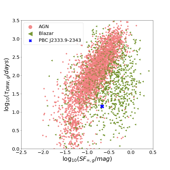
Figure 5: Distribution of the Damp Random Walk (DRW) parameters, $\tau_{DRW}$ (in days) against $SF_{\infty}$ (in $mag$), in logarithmic scale, in the g-filter for the ALeRCE training set sample of non-blazar AGN (red circles) and blazars (green triangles). The parameters for PBC J2333.9-2343 are marked as a blue cross.

4.2 Constraints on the region responsible for the variations observed in the optical/NIR bands

Optical and NIR variations are normally seen in radio quiet AGN as well as radio loud objects. In the former case they are often attributed to variations in the accretion disc (optical and NIR) and reprocessing of variable emission in the torus (NIR). In this section we compare the upper limits on the delay between I band and K band fluctuations in PBC J2333.9-2343 to the ranges of delays expected in these non-jet scenarios, in order to constrain the origin of the variable optical/NIR emission in this object. In PBC J2333.9-2343 we found a time lag between the K and I band of 1.02$\pm$1.45 days, so we can investigate if the lag would be compatible with the K band emission arising from the torus, the accretion disk or the jet. We use a black hole mass of logM_BH = 8.4 and the luminosity at 5100 Å reported in Hernández-García et al. (2018) to estimate an Eddington ratio $R_{\rm Edd}$ of 3.2$\times$10^-3 following Sánchez-Sáez et al. (2018).

When the NIR emission is dominated by the torus, the dust, responsible for the re-emission in the NIR, can only be located at distances of at least light days/weeks, so variations may occur smoothly and with time lags of weeks/months due to the different time delays on different sides of the torus (Lira et al., 2015; Sánchez et al., 2017). Indeed, recent studies show delayed response of the K-band light curve after the V-band light curve of at least 10 days, and in particular for the luminosity of PBC J2333.9-2343 a lag longer than 80 days is expected (Koshida et al., 2014; Minezaki et al., 2019). We can therefore reject that the torus is responsible for the NIR emission.

The variable optical and NIR emission can also come from the accretion disk, either through intrinsic (i.e. viscosity or thermal) changes in the disk or through reprocessing of a variable illuminating source, for example of X-rays (Netzer, 2013). In the first case, the intrinsic variations have difficulty reproducing quasi-simultaneous flux changes in two different bands, unless it is only a small region of the disk which is varying and this region contributes all the variability of both bands even if it does not produce all their emission. In any accretion disk where the surface temperature decreases outwards, longer wavelength are emitted by larger fractions of the disk. Therefore, if only a small central region of the disk is producing the variations, these will modulate a larger fraction of the total I band emission than of the total emission of the disk in the K band and the fractional variability of the I band would be larger than that of the K band, which is contrary to what we observe. On the other hand, to estimate the delay expected from reprocessing on the disk, we followed Lira et al. (2015) to estimate the light travel time across a standard accretion disk model as $\tau=3\times 10^{-10}\lambda^{4/3}R_{Edd}^{1/3}M_{BH}^{2/3}$, with $\lambda$ in Å, $\tau$ in days, $R_{Edd}$ in Eddington units and M_BH in solar masses. The expected lag between the K and I band is of 7.5 days, much larger than the measured value of $1.02\pm{1.45}$ days. Thus it is unlikely that the accretion disk is responsible for the variable emission in both I and K bands.

If variations are related to jet emission and the jet is oriented towards the observer, however, the variability timescale is shortened and the radiation is strongly enhanced by relativistic beaming. The characteristic timescales of such variations are of about a few days, which may be interpreted as the typical timescale of successive flare events (Kataoka et al., 2001). In fact, if the emission is dominated by emission from the jet both at optical and NIR frequencies, then the variations are rapid, high amplitude and simultaneous in both bands (Asmus et al., 2015). For instance, Bonning et al. (2012) presented the results of light curves from a sample of 12 blazars observed by SMARTS-1.3m in the BVRJK between 2008-10, showing that their CCFs are centered around zero. The monitoring campaign presented here, as well as the analysis of the variability in PBC J2333.9-2343 (see Sect. 3.1), reveals large amplitude variations at short timescales showing flaring behaviour, and the fact that the variations occur simultaneously in the optical and NIR band agrees well with the blazar nature of PBC J2333.9-2343.

The doubling/halving times were estimated to be 7.7 days (I band) and 6.7 days (K band). We estimated the electrons cooling time in the observer frame using best fit parameters for the SED from 2018-19, taking into account both synchrotron and IC/EC in Thomson regime, which results to be $\sim$0.3 days, and the escape time, ignoring possible contribution from turbulence, ($\frac{R(1+z)}{c\delta_{D}}$) $\sim$ 1 day. This seems to indicate that the decay could be driven not only by the electrons cooling/escape times, but other mechanisms may play a role, as for instance a modulation in the injection of the particles (and/or in the beaming pattern), or an area of magnetic reconnection in the flare (see e.g., Zhu et al., 2018; Sahakyan et al., 2020; Pandey & Stalin, 2022).

4.3 Multiwavelength emission

Extra-galactic emission in the gamma-ray band is a phenomenon related to the presence of relativistic jets (Dermer & Giebels, 2016). PBC J2333.9-2343 is detected by Fermi-LAT and reported in the fourth catalog of AGN detected by the Fermi Gamma-ray Space Telescope Large Area Telescope (4LAC), with an integrated flux of 3.9$\pm$0.5$\times$10^-12 erg s^-1cm^-2 in the 0.1-100 GeV band between 2008 and 2016, and a spectral index of 2.42$\pm$0.12 (Ajello et al., 2020), in agreement with our results (see Sect. 2.6). Indeed, this source is classified as a remarkable ‘other AGN’ case because it was not possible to classify it. We notice that the fact that gamma-ray emission was detected on this source with Fermi-LAT at a 6.2$\sigma$ of significance level is more likely indicative to be from a blazar rather than a radio galaxy. Furthermore, our results show that this source has varied in the gamma-ray range, the number of photons being almost half in 2015 compared to the 2018-2019 data. This is in agreement with the variability results from the 4FGL-DR3 where a variability index of 30.8 is reported for this source (Abdollahi et al., 2022).

Blazars characteristically show a two hump structure (low and high energy), as we see for PBC J2333.9-2343. The low energy hump is well explained by synchrotron emission by ultrarelativistic electrons, whereas the high peak is usually interpreted as inverse Compton (IC) emission for the case of a pure leptonic scenario (Blandford & Königl, 1979), or dominated by high energy emission of ultra-relativistic protons in the case of the hadronic scenario (Dermer & Schlickeiser, 1993; Böttcher et al., 2013). Radio galaxies can also show a two hump structure, the way to differentiate between a blazar or a radio galaxy being the jet angle (e.g., Ghisellini et al., 2005). In this work we used a one-zone leptonic model, where the high energy frequencies are well fitted by EC emission and some SSC contribution, with values of the model parameters within the blazar expectations, among them a jet angle of 3 degrees (see Fig. 4 and Table 2).

A previous SED fitting was presented in Hernández-García et al. (2017) using simultaneous XMM–Newton data. The main difference between the SED fittings is that in Hernández-García et al. (2017) the SSC and EC are fitted separately, whereas here they are fitted simultaneously. Moreover, the photon contribution to the EC model in Hernández-García et al. (2017) comes from IC emission with seed photons from the torus, whereas in this work the contribution comes from IC emission with seed photons from the disk, the BLR and the torus.

In order to be able to compare the SEDs built in 2015 and 2018, we fitted the two of them with the same model (see Section 3.3). The main result from this analysis is that the jet angle must be very close to the line of sight of the observer. For larger angles the Doppler boosting is smaller and therefore in order to properly fit the lower frequency peak of the SED it becomes necessary to either increase the energy of the electron population, or increase the amount of electrons available (either by increasing the density or the size of the region). However, for both cases, the high energy part of the SED model increases significantly, which results in a poor fit to the X-ray data. Therefore, we found necessary to increase the Doppler boosting (lowering the angle) to obtain a good fit.

The advantage of the current SED is that more data points are available, including data in the gamma-rays, which allows a more robust fit. In particular, the fact that gamma-ray emission is detected and the SED shows a two peaked structure favors the blazar-like nature hypothesis, consistent with its variability pattern. It is worth remarking that according to the SED modeling, in this object, the contribution of the disk and the torus is negligible compared to the synchrotron emission, which would be responsible for almost all the optical and NIR emission, as well as the X-rays and gamma-rays can also be explained by emission reprocessed by the jet, with mild contribution from the dusty torus.

Blazars are further classified into flat-spectrum radio quasars (FSRQ) and BL Lac (BL Lacertae being the prototype) based on various observational properties. BL Lacs show no (or weak) emission lines in their optical spectra, and the synchrotron peaks in the SED at frequencies $>$ 10¹⁴ Hz, whereas FSRQ do show emission lines and their synchrotron typically peaks at frequencies lower than 10¹⁴ Hz (Abdo et al., 2010; Giommi et al., 2012b; Padovani et al., 2017). The optical spectrum of PBC J2333.9-2343 shows prominent narrow and broad emission lines (Hernández-García et al., 2018) and the synchrotron peak in the SED is at $<$ 10¹⁴ Hz (Fig. 4), therefore we classify the nucleus of this galaxy as a FSRQ.

We would like to stress the peculiarities of this galaxy, with emphasis on the low gamma-ray luminosity ((3.10$\pm$0.02)$\times$10⁴³ erg $s^{-1}$) compared to other blazars (see Fig. 10 in Ajello et al., 2020), more typical of BL Lacs. It has also being suggested that BL Lacs are dominated by SSC whereas FSRQ are dominated by EC, in agreement with the classical FSRQ classification of PBC J2333.9-2343. However, there are examples in the literature of sources that can change from EC to SSC dominated, as for example 3C 279 (Patiño-Álvarez et al., 2018). In the recent work by Pei et al. (2022) the authors proposed an “appareling zone” consisting on a potential transition field between BL Lacs and FSRQs where changing-look blazars may reside based on four physical parameters, where PBC J2333.9-2343 indeed should be located. Other examples of sources showing observational characteristics changing between a BL Lac and a FSRQ include BS B1646+499 (Pajdosz-Śmierciak et al., 2018) or B2 1420+32 (Mishra et al., 2021). Observing morphologically different AGN types simultaneously has been proposed as the result of jet axis reorientation (Pajdosz-Śmierciak et al., 2022). PBC J2333.9-2343 could also be an extreme case of XRG, with the new jet pointing towards us and therefore preventing us from observing the X-shaped morphology.

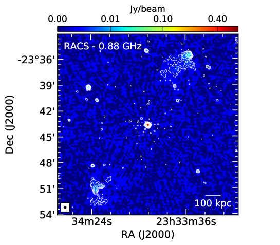
Figure 6: Image of PBC J2333.9-2343 from the RACS survey at 0.88 GHz. Contours are 3$\times$RMS$\times$(-1, 1, 2, 4, 8, 16, 32, 64, 128, 256). The HPBW (14.8″$\times$13.5″) is shown in the lower-left corner.

4.4 Radio morphology and long-term variability from the latest radio surveys and archives

An additional evidence in favour of the blazar nature of the core is the lack of clear jet emission connecting the lobes and the core region presented in Bruni et al. (2020) with the GMRT at 150 MHz. To further confirm this result, we considered images of the source from recently released radio surveys: the VLASS at 3 GHz, and the RACS at 0.88 GHz. The latter has a sensitivity ten times larger than the mentioned GMRT observations, and five times larger than the NVSS. Moreover, the short baselines of ASKAP allow to recover extended structures up to 1 deg, making it suitable for the study of GRGs. The RACS image is presented in Figure 6: at a noise level of 215 $\mu$Jy/beam, and a resolution of $\sim$15″, no sign of connection between the lobes and the nucleus is visible, confirming previous results. The shortest distance between the core and the first contour of the lobes is $\sim$3′ (167 kpc at the redshift of the source), resulting in a missing association and the consequent absence of this source in the recent catalogue of GRG from RACS (Andernach et al., 2021). The VLASS quick-look image, at an angular resolution of $\sim$2.8 arcsec and an RMS of 580 $\mu$Jy/beam, detects only the core. This is expected, since the VLA configuration used for the survey (B) only allows to recover structures with an angular size up to 1′. However, the absence of a jet even in the regions closer to the core, confirms the discontinuity visible at lower frequencies.

Finally, we have investigated the core long-term radio variability browsing the NRAO VLA archive survey (NVAS, Crossley et al. 2007). We could collect images between 1983 and 2001, covering almost 20 years at 4.8 and 15 GHz. At 8.5 GHz, the observations span about 10 years (1990-1999). The highest flux density was recorded at 15 GHz during November 1984 (6.9$\pm$0.3 Jy), corresponding to a factor of $\sim$ 7 of variability with respect to previous and subsequent epochs. A corresponding, although lower, peak is present at 4.8 GHz (200% increase, also November 1984), confirming the variation. Only mild variations were recorded at these frequencies during later years. At 8.5 GHz, the absolute maximum was recorded in July 1991 (an increase of a factor 2 with respect to the previous epoch), and milder variations during 1999. As a whole, these archival data confirm the pronounced variability discussed in this work, and detected in the radio band with the Effelsberg observations on a shorter time window, as well as comparison with previous works such as the flux reported at 8 GHz by Ojha et al. (2004) and Hernández-García et al. (2017) with data obtained 11 years later.

4.5 A re-oriented jet or an intervening blazar in a GRG?

Another possibility to explain the behaviour of this source is to consider the presence of an intervening blazar in our line of sight. Looking at the number of hard X-ray selected blazars, N, as a function of flux, S (14-195 keV), logN-logS (see figure 10 from Langejahn et al. 2020) and assuming the Swift/XRT error circle of 6 arcsec, the number of blazars similar to PBC J2333.9-2343 expected to fall in it is $\sim$6$\times$10^-5, i.e. indicating that a chance overlap is unlikely.

Generally in these cases there is an overlapping of two different optical spectra with some peculiar composition, as for instance lines at different redshift, that should appear as double peaked lines in the narrow emission lines. This is not observed in the spectra of PBC J2333.9-2343  even with data obtained from the Very Large Telescope at a dispersion of 0.3 Å/pixel (Hernandez-Garcia et al., in prep.). Then, if there are two sources we should assume that there is a broad-line radio galaxy with its optical spectrum and then a blazar with a featureless blue spectrum which becomes embedded in the radio galaxy. However, no indications of composite spectral continuum are found.

If an intervening blazar can be discarded, we can conclude that the GRG and the blazar nucleus in PBC J2333.9-2343 are part of the same galaxy. Then, the most plausible explanation is that the jet has changed its direction, as previously proposed in Hernández-García et al. (2017), making this an exceptional case of jet reorientation. These kind of changes have already been proposed to explain XRGs. For example, Dennett-Thorpe et al. (2002) studied two XRG (3C 223.1 and 3C 403) and explained the morphology in terms of a rapid realignment of the radio jet, and considered a binary black hole merger or acquisition of a smaller galaxy as likely candidates for the cause of the change of the jet axis, as they did not see any indication of merging. Similarly, Machalski et al. (2016) reported the case of 3C 293, which is very likely the result of a post merging event with the galaxy UGC 8782. In this work they concluded that the jet axis flipped rapidly due to tidal interaction of its merging process. In the particular case of PBC J2333.9-2343, we do not see the X-shape, but this can be explained because the new jets are, by chance, pointing towards us. The confirmation of no emission between the nucleus and the jet discussed in Sect. 4.4 strongly supports the idea of a re-oriented jet.

5 Conclusions

In this work we presented a contemporaneous multiwavelength monitoring of the nucleus in PBC J2333.9-2343 that covered two periods, between September 2018 and January 2019, and April-July 2019. Variations are found at all observed wavelengths at significance larger than 6$\sigma$, except at X-rays where variations are detected at 2$\sigma$ of confidence level within the four month monitoring period. The observed variations occur in timescales shorter than a month and with amplitudes larger than a factor of two. The cross-correlation between optical/NIR also shows that the variations occur simultaneously in these bands. When comparing the optical variability features with large samples of non-blazar AGN and blazars, PBC J2333.9-2343 shows characteristics more similar to the blazar population. According to these results, we interpret the observed variations as flaring events.

We constructed the SED, that we then fitted using a single-zone leptonic model. The SED shows two distinct peaks, the low energy one is well fitted by synchrotron emission, while the high energy peak is dominated by EC from the torus with some contribution from SSC. This SED was compared with the data already presented in Hernández-García et al. (2017) using VLBA and XMM-Newton, and we added Fermi-LAT data. The jet angle in the fitted models is 3 degrees, indicative of a blazar.

These results and the gamma-ray detection at 6$\sigma$ of confidence level strongly suggest the presence of a blazar-like nucleus at the center of PBC J2333.9-2343. This galaxy was previously classified as a GRG, suggestive of a change in the direction of the jet as previously proposed in Hernández-García et al. (2017). Further evidence in agreement with this scenario is the fact that no connection between the nucleus and the lobes is observed in the deepest radio images, and historical radio fluxes from the NRAO VLA archive survey revealed variations by a factor of seven about 30 years ago, confirming the pronounced variability in the radio at 20.4 GHz shown in the present work.

In the future we can use resources such as the ZTF or ATLAS alert streams to monitor this or other interesting sources and trigger other instrumentation at different wavebands when a flaring event is detected. In particular, ALeRCE has a watchlist service that notifies via email when a source from your own target list generates an alert.

Data availability

The data underlying this article were accessed from the ZTF Forced Photometry Service (https://ztfweb.ipac.caltech.edu/cgi-bin/requestForcedPhotometry.cgi), the ATLAS Forced Photometry Service (https://fallingstar-data.com/forcedphot/), Swift (https://swift.gsfc.nasa.gov/), and Fermi (https://fermi.gsfc.nasa.gov/) archives. The Effelsberg, VLBA, SMARTS-1.3m data and the derived data generated in this research will be shared on reasonable request to the corresponding author.

Appendix A Figures and tables

In this section we present the plots and tables of the monitoring campaigns with the different instruments. In Fig. 7 and Table 3, results of the radio monitoring performed with the Effelsberg-100m single dish at 4.8, 8.5, 10.5, and 20.4 GHz are shown. Details about receivers and instrumental setup are reported in Table 4. In Table 5 we report information about the VLBA observations. Fig. 8 and Table LABEL:tab:smarts show fluxes of the NIR ($K$-band) and optical ($V$/$I$ bands) from the SMARTS-1.3m. Optical data are shown also in Fig. 9 and Table LABEL:tab:ztf for ZTF in the gri filters, and in Fig. 10 and Table LABEL:tab:atlas for ATLAS in the oc filters. Swift data is presented in Table 9 and Figs. 11 (UVM2 filter) and 12 (X-rays).

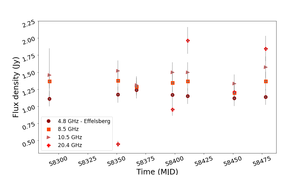
Figure 7: Effelsberg radio flux densities collected from June to December 2018, at 4.8, 8.5, 10.5, and 20.4 GHz.

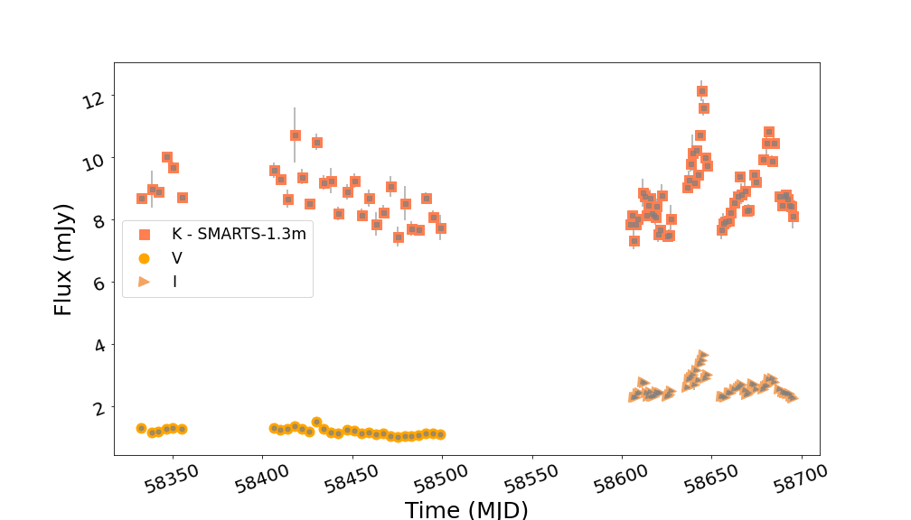
Figure 8: Flux light curves in $V$ and $I$ bands and the corresponding simultaneous $K$ band light curves with SMARTS-1.3m.

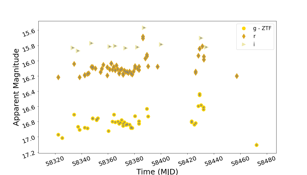
Figure 9: ZTF forced photometry light curves in the gri filters between July 2018 and January 2019.

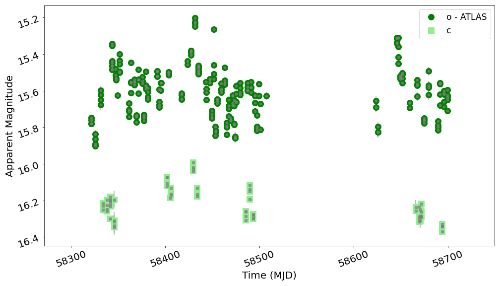
Figure 10: ATLAS forced photometry light curves in the c and o filters between July 2018 and May 2019.

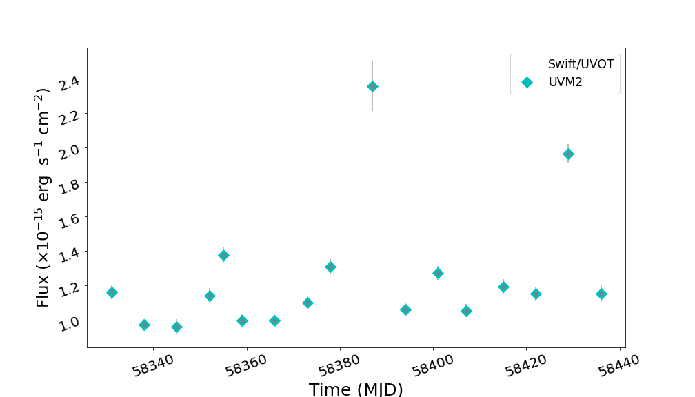
Figure 11: Swift/UVOT lightcurve of the observations during weekly monitoring between August-November 2018.

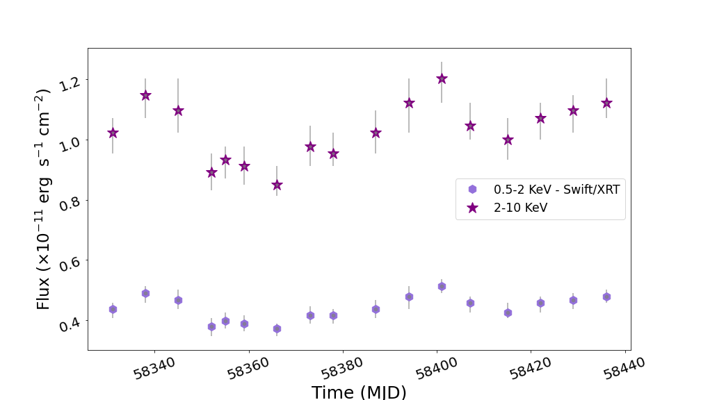
Figure 12: Swift/XRT lightcurves of PBC J2333.9-2343 in the soft (0.5-2 keV) and hard (2-10 keV) energy bands during the weekly monitoring between August-November 2018.

Table 3: Flux densities between 4.8 and 20.4 GHz, collected at the different epochs (in MJD) with the Effelsberg-100m telescope.

MJD	$S_{4.8}$	$S_{8.5}$	$S_{10.5}$	$S_{20.4}$
	(Jy)	(Jy)	(Jy)	(Jy)
58293	1.1$\pm$0.1	1.4$\pm$0.1	1.5$\pm$0.4	–
58351	1.2$\pm$0.1	1.4$\pm$0.1	1.5$\pm$0.2	0.45$\pm$0.05
58367	1.2$\pm$0.1	1.3$\pm$0.1	1.3$\pm$0.1	–
58398.9	1.2$\pm$0.1	1.3$\pm$0.1	1.5$\pm$0.2	0.96$\pm$0.09
58411.9	1.2$\pm$0.1	1.4$\pm$0.1	1.5$\pm$0.2	2.0$\pm$0.2
58451.7	1.1$\pm$0.1	1.2$\pm$0.1	1.3$\pm$0.1	1.2$\pm$0.1
58478.7	1.1$\pm$0.1	1.4$\pm$0.1	1.6$\pm$0.2	1.8$\pm$0.2

Table 4: Log of used receivers at the Effelsberg-100m telescope.

	S60mm	S36mm	S28mm	S14mm
Center frequency	4.85 GHz	8.35 GHz	10.45 GHz	20.40 GHz
Typical $T_{sys}$ (zenith)	25 K	22 K	50 K	51 K
HPBW	145 arcsec	82 arcsec	66 arcsec	40 arcsec
Sensitivity	1.55 K/Jy	1.35 K/Jy	1.35 K/Jy	1.07 K/Jy
N. of pixels	2	1	2	1

Table 5: VLBA images parameters. Column 1: frequency, Col. 2: full width at half maximum (FWHM) with position angle, Col. 3: image noise, Col. 4: image peak brightness, Col. 6: total flux density.

$\nu$	FWHM	RMS	$I_{\nu}$	$S_{\nu}$
(GHz)	(mas$\times$mas, deg)	(mJy/beam)	(mJy/beam)	(Jy)
15	0.9$\times$0.3, –2.2	0.3	1072	1.7$\pm$0.2
24	0.6$\times$0.2, –3.4	1.3	911	1.4$\pm$0.1

Table 6: A Log of the SMARTS-1.3m observations. This includes dates in MJD, and the fluxes in the optical and NIR bands (in mJy). In the optical, dates before MJD=58499 are in the $V$-filter, and after that in the $I$-filter.

MJD	Flux ($V$/$I$) mJy	Flux ($K$) mJy
58332.3	1.31 $\pm$ 0.02	8.69 $\pm$ 0.09
58338.3	1.150 $\pm$ 0.005	9.0 $\pm$ 0.6
58342.2	1.184 $\pm$ 0.003	8.9 $\pm$ 0.1
58346.2	1.266 $\pm$ 0.008	10.02 $\pm$ 0.08
58350.2	1.31 $\pm$ 0.02	9.7 $\pm$ 0.2
58355.2	1.27 $\pm$ 0.02	8.7 $\pm$ 0.1
58406.2	1.301 $\pm$ 0.005	9.6 $\pm$ 0.2
58410.1	1.24 $\pm$ 0.03	9.32 $\pm$ 0.09
58414.1	1.3 $\pm$ 0.1	8.7 $\pm$ 0.3
58418.1	1.35 $\pm$ 0.04	10.7 $\pm$ 0.9
58422.2	1.266 $\pm$ 0.003	9.5 $\pm$ 0.3
58426.1	1.180 $\pm$ 0.003	8.530 $\pm$ 0.007
58430.1	1.50 $\pm$ 0.01	10.5 $\pm$ 0.3
58434.1	1.260 $\pm$ 0.007	9.2 $\pm$ 0.2
58438.1	1.16 $\pm$ 0.01	9.3 $\pm$ 0.4
58442.1	1.136 $\pm$ 0.005	8.2 $\pm$ 0.2
58447.1	1.24 $\pm$ 0.02	8.9 $\pm$ 0.3
58451.1	1.212 $\pm$ 0.004	9.2 $\pm$ 0.2
58455.1	1.128 $\pm$ 0.004	8.1 $\pm$ 0.2
58459.1	1.157 $\pm$ 0.002	8.7 $\pm$ 0.3
58463.1	1.093 $\pm$ 0.008	7.9 $\pm$ 0.4
58467.0	1.140 $\pm$ 0.004	8.2 $\pm$ 0.2
58471.1	1.050 $\pm$ 0.004	9.1 $\pm$ 0.3
58475.1	1.014 $\pm$ 0.008	7.4 $\pm$ 0.3
58479.1	1.048 $\pm$ 0.007	8.5 $\pm$ 0.5
58483.0	1.040 $\pm$ 0.004	7.7 $\pm$ 0.2
58487.0	1.083 $\pm$ 0.004	7.69 $\pm$ 0.05
58491.0	1.120 $\pm$ 0.007	8.7 $\pm$ 0.2
58495.0	1.12 $\pm$ 0.03	8.1 $\pm$ 0.2
58499.0	1.12 $\pm$ 0.03	7.7 $\pm$ 0.4
58606.4	2.29 $\pm$ 0.02	7.9 $\pm$ 0.2
58607.4	2.30 $\pm$ 0.03	8.2 $\pm$ 0.1
58608.4	2.42 $\pm$ 0.02	7.3 $\pm$ 0.3
58609.4	2.44 $\pm$ 0.03	7.9 $\pm$ 0.2
58611.4	2.77 $\pm$ 0.04	8.0 $\pm$ 0.2
58612.4	2.763 $\pm$ 0.008	8.9 $\pm$ 0.4
58613.4	2.4 $\pm$ 0.1	8.8 $\pm$ 0.2
58614.4	2.32 $\pm$ 0.03	8.1 $\pm$ 0.1
58615.4	2.472 $\pm$ 0.007	8.48 $\pm$ 0.09
58616.4	2.33 $\pm$ 0.01	8.7 $\pm$ 0.2
58617.4	2.32 $\pm$ 0.01	8.2 $\pm$ 0.2
58618.4	2.38 $\pm$ 0.03	8.2 $\pm$ 0.3
58619.4	2.47 $\pm$ 0.04	8.1 $\pm$ 0.3
58620.4	2.42 $\pm$ 0.02	8.4 $\pm$ 0.3
58621.4	2.43 $\pm$ 0.01	7.6 $\pm$ 0.3
58625.4	2.321 $\pm$ 0.008	7.69 $\pm$ 0.08
58626.4	2.39 $\pm$ 0.02	8.8 $\pm$ 0.3
58627.4	2.48 $\pm$ 0.07	7.48 $\pm$ 0.07
58636.4	2.60 $\pm$ 0.01	7.5 $\pm$ 0.2
58637.4	2.87 $\pm$ 0.02	8.0 $\pm$ 0.4
58638.4	2.91 $\pm$ 0.02	9.1 $\pm$ 0.1
58639.4	3.01 $\pm$ 0.03	9.3 $\pm$ 0.3
58640.4	2.7 $\pm$ 0.2	9.8 $\pm$ 0.3
58641.3	3.16 $\pm$ 0.08	10.2 $\pm$ 0.6
58642.4	2.85 $\pm$ 0.02	9.20 $\pm$ 0.02
58643.4	3.35 $\pm$ 0.04	10.2 $\pm$ 0.2
58644.4	3.48 $\pm$ 0.02	9.4 $\pm$ 0.1
58645.4	3.64 $\pm$ 0.08	10.7 $\pm$ 0.1
58646.4	2.90 $\pm$ 0.03	12.1 $\pm$ 0.3
58647.4	3.01 $\pm$ 0.02	11.6 $\pm$ 0.3
58655.3	2.31 $\pm$ 0.08	10.0 $\pm$ 0.1
58656.4	2.31 $\pm$ 0.02	9.8 $\pm$ 0.1
58657.4	2.30 $\pm$ 0.03	7.7 $\pm$ 0.3
58659.4	2.43 $\pm$ 0.01	7.9 $\pm$ 0.3
58660.4	2.43 $\pm$ 0.01	7.93 $\pm$ 0.07
58662.4	2.56 $\pm$ 0.04	7.9 $\pm$ 0.2
58664.3	2.58 $\pm$ 0.03	8.24 $\pm$ 0.08
58665.4	2.629 $\pm$ 0.008	8.57 $\pm$ 0.06
58666.4	2.70 $\pm$ 0.02	8.7 $\pm$ 0.1
58668.4	2.53 $\pm$ 0.03	9.4 $\pm$ 0.1
58669.4	2.384 $\pm$ 0.004	8.8 $\pm$ 0.3
58670.4	2.43 $\pm$ 0.01	8.9 $\pm$ 0.3
58672.4	2.73 $\pm$ 0.02	8.29 $\pm$ 0.04
58673.4	2.70 $\pm$ 0.04	8.3 $\pm$ 0.2
58674.4	2.56 $\pm$ 0.02	9.5 $\pm$ 0.1
58678.4	2.540 $\pm$ 0.004	9.2 $\pm$ 0.1
58679.4	2.642 $\pm$ 0.007	9.9 $\pm$ 0.1
58680.4	2.67 $\pm$ 0.02	10.5 $\pm$ 0.4
58681.4	2.86 $\pm$ 0.01	10.84 $\pm$ 0.08
58683.4	2.90 $\pm$ 0.03	9.9 $\pm$ 0.2
58684.4	2.78 $\pm$ 0.01	10.5 $\pm$ 0.2
58687.3	2.55 $\pm$ 0.08	8.8 $\pm$ 0.1
58689.3	2.476 $\pm$ 0.006	8.5 $\pm$ 0.1
58690.4	2.43 $\pm$ 0.03	8.8 $\pm$ 0.2
58691.3	2.426 $\pm$ 0.006	8.8 $\pm$ 0.1
58692.3	2.40 $\pm$ 0.01	8.68 $\pm$ 0.09
58693.3	2.41 $\pm$ 0.01	8.5 $\pm$ 0.2
58694.3	2.312 $\pm$ 0.005	8.4 $\pm$ 0.1
58695.3	2.27 $\pm$ 0.02	8.1 $\pm$ 0.4

Table 7: Log of the ZTF forced photometry observations. Include the dates in MJD, filter, and color corrected apparent magnitudes.

MJD	Filter	Magnitude (mag)
58322.439	g	16.969$\pm$0.006
58322.481	r	16.215$\pm$0.004
58325.417	g	17.01$\pm$0.03
58333.399	i	15.831$\pm$0.005
58334.418	r	16.041$\pm$0.005
58334.46	g	16.71$\pm$0.01
58337.396	g	16.867$\pm$0.006
58337.460	i	15.869$\pm$0.005
58338.408	g	16.908$\pm$0.006
58338.463	r	16.217$\pm$0.006
58342.416	g	16.878$\pm$0.006
58342.501	r	16.186$\pm$0.006
58342.502	r	16.194$\pm$0.008
58344.397	g	16.885$\pm$0.005
58344.420	r	16.174$\pm$0.004
58345.376	r	16.163$\pm$0.004
58347.376	i	15.769$\pm$0.005
58347.398	r	16.079$\pm$0.003
58348.369	g	16.757$\pm$0.005
58348.370	g	16.760$\pm$0.005
58348.398	r	16.079$\pm$0.003
58348.398	r	16.092$\pm$0.003
58350.377	r	16.101$\pm$0.003
58351.399	g	16.770$\pm$0.004
58351.400	g	16.781$\pm$0.005
58352.355	g	16.75$\pm$0.01
58354.377	r	16.148$\pm$0.008
58355.349	r	16.11$\pm$0.01
58356.382	r	16.05$\pm$0.01
58359.367	r	16.09$\pm$0.01
58359.368	r	16.19$\pm$0.01
58360.372	g	16.92$\pm$0.02
58361.354	r	16.113$\pm$0.007
58361.356	i	15.814$\pm$0.006
58362.334	r	16.036$\pm$0.004
58362.335	r	16.035$\pm$0.004
58363.337	g	16.799$\pm$0.009
58363.423	r	16.116$\pm$0.005
58364.349	r	16.080$\pm$0.005
58364.398	g	16.708$\pm$0.009
58365.326	i	15.806$\pm$0.005
58365.355	r	16.126$\pm$0.005
58365.356	r	16.125$\pm$0.004
58365.398	g	16.807$\pm$0.007
58366.350	r	16.061$\pm$0.003
58367.336	r	16.110$\pm$0.004
58367.397	g	16.799$\pm$0.005
58368.334	r	16.161$\pm$0.004
58368.335	r	16.168$\pm$0.003
58368.356	g	16.825$\pm$0.005
58369.331	g	16.811$\pm$0.006
58369.357	r	16.121$\pm$0.005
58370.307	r	16.110$\pm$0.005
58370.350	g	16.779$\pm$0.006
58371.320	r	16.167$\pm$0.003
58371.322	r	16.185$\pm$0.003
58371.335	g	16.829$\pm$0.006
58371.352	g	16.856$\pm$0.005
58372.373	r	16.129$\pm$0.004
58372.400	g	16.809$\pm$0.007
58373.309	r	16.145$\pm$0.005
58373.335	i	15.835$\pm$0.007
58373.358	g	16.841$\pm$0.007
58374.334	r	16.145$\pm$0.004
58374.335	r	16.148$\pm$0.004
58374.414	g	16.829$\pm$0.008
58374.415	g	16.840$\pm$0.008
58375.354	r	16.159$\pm$0.004
58376.312	g	16.839$\pm$0.006
58376.337	r	16.141$\pm$0.004
58377.293	r	16.163$\pm$0.005
58377.310	r	16.170$\pm$0.004
58377.337	g	16.884$\pm$0.007
58377.338	g	16.870$\pm$0.007
58378.287	r	16.182$\pm$0.005
58378.314	g	16.881$\pm$0.007
58379.313	r	16.141$\pm$0.005
58380.293	r	16.093$\pm$0.005
58380.294	r	16.070$\pm$0.005
58380.337	g	16.726$\pm$0.008
58382.273	i	15.820$\pm$0.006
58382.314	r	16.101$\pm$0.008
58383.272	g	16.80$\pm$0.02
58383.274	g	16.83$\pm$0.02
58383.294	r	16.12$\pm$0.01
58383.295	r	16.08$\pm$0.01
58386.293	r	15.705$\pm$0.009
58386.298	r	15.68$\pm$0.01
58387.355	i	15.567$\pm$0.009
58388.271	r	15.969$\pm$0.008
58389.265	r	15.922$\pm$0.006
58389.266	r	15.940$\pm$0.006
58389.343	g	16.631$\pm$0.013
58390.270	r	16.074$\pm$0.006
58390.300	g	16.73$\pm$0.01
58397.283	r	16.079$\pm$0.004
58397.284	r	16.077$\pm$0.004
58400.231	i	15.785$\pm$0.005
58423.214	g	16.81$\pm$0.01
58423.214	g	16.79$\pm$0.01
58425.186	g	16.841$\pm$0.009
58426.226	g	16.82$\pm$0.01
58426.234	r	16.143$\pm$0.009
58426.235	r	16.157$\pm$0.009
58428.187	g	16.597$\pm$0.006
58428.250	r	15.933$\pm$0.005
58429.23	g	16.436$\pm$0.006
58429.247	g	16.453$\pm$0.006
58429.254	r	15.841$\pm$0.004
58429.255	r	15.841$\pm$0.004
58430.210	i	15.704$\pm$0.006
58430.262	g	16.582$\pm$0.007
58431.188	r	15.809$\pm$0.008
58432.231	g	16.610$\pm$0.009
58432.243	g	16.638$\pm$0.009
58432.254	r	15.945$\pm$0.007
58432.255	r	15.986$\pm$0.007
58434.210	i	15.821$\pm$0.009
58457.171	r	16.20$\pm$0.01
58472.165	g	17.10$\pm$0.03

Table 8: Log of the ATLAS forced photometry observations. Includes dates in MJD, filter, and magnitudes.

MJD	Filter	Magnitude (mag)
58321.519	o	15.76$\pm$0.01
58321.527	o	15.78$\pm$0.01
58321.535	o	15.78$\pm$0.01
58321.542	o	15.75$\pm$0.01
58325.452	o	15.86$\pm$0.02
58325.460	o	15.90$\pm$0.02
58325.469	o	15.89$\pm$0.02
58325.477	o	15.84$\pm$0.02
58331.508	o	15.65$\pm$0.03
58331.511	o	15.68$\pm$0.03
58331.524	o	15.62$\pm$0.02
58331.533	o	15.60$\pm$0.02
58333.608	c	16.22$\pm$0.02
58333.616	c	16.23$\pm$0.02
58333.625	c	16.25$\pm$0.02
58337.497	c	16.23$\pm$0.01
58337.510	c	16.19$\pm$0.01
58337.512	c	16.25$\pm$0.01
58337.521	c	16.26$\pm$0.01
58341.489	c	16.20$\pm$0.01
58341.498	c	16.20$\pm$0.01
58341.507	c	16.22$\pm$0.01
58341.509	c	16.20$\pm$0.01
58341.512	c	16.18$\pm$0.01
58341.515	c	16.23$\pm$0.01
58341.521	c	16.30$\pm$0.01
58343.486	o	15.46$\pm$0.01
58343.497	o	15.44$\pm$0.01
58343.499	o	15.48$\pm$0.01
58343.501	o	15.47$\pm$0.01
58343.503	o	15.35$\pm$0.01
58343.510	o	15.45$\pm$0.01
58343.511	o	15.34$\pm$0.01
58343.520	o	15.49$\pm$0.01
58345.486	c	16.35$\pm$0.04
58345.492	c	16.34$\pm$0.04
58345.499	c	16.31$\pm$0.03
58345.516	c	16.20$\pm$0.05
58345.517	c	16.31$\pm$0.05
58347.467	o	15.48$\pm$0.01
58347.476	o	15.52$\pm$0.01
58347.491	o	15.53$\pm$0.01
58347.500	o	15.540$\pm$0.009
58349.566	o	15.63$\pm$0.01
58351.518	o	15.40$\pm$0.01
58351.520	o	15.46$\pm$0.01
58351.528	o	15.50$\pm$0.01
58351.530	o	15.44$\pm$0.01
58351.538	o	15.50$\pm$0.01
58351.548	o	15.50$\pm$0.01
58361.452	o	15.71$\pm$0.01
58361.455	o	15.70$\pm$0.01
58361.464	o	15.74$\pm$0.01
58361.465	o	15.71$\pm$0.01
58363.437	o	15.55$\pm$0.01
58363.453	o	15.61$\pm$0.01
58363.463	o	15.45$\pm$0.01
58363.466	o	15.56$\pm$0.01
58367.436	o	15.551$\pm$0.009
58367.453	o	15.551$\pm$0.009
58367.461	o	15.538$\pm$0.009
58367.463	o	15.568$\pm$0.009
58369.431	o	15.77$\pm$0.01
58369.439	o	15.74$\pm$0.01
58369.440	o	15.74$\pm$0.01
58369.454	o	15.74$\pm$0.01
58371.429	o	15.49$\pm$0.01
58371.430	o	15.54$\pm$0.01
58371.441	o	15.61$\pm$0.01
58371.456	o	15.54$\pm$0.01
58375.426	o	15.546$\pm$0.009
58375.435	o	15.60$\pm$0.01
58375.436	o	15.52$\pm$0.01
58377.467	o	15.74$\pm$0.01
58377.478	o	15.75$\pm$0.01
58377.487	o	15.73$\pm$0.01
58377.498	o	15.76$\pm$0.01
58379.458	o	15.50$\pm$0.02
58379.468	o	15.57$\pm$0.02
58379.478	o	15.59$\pm$0.02
58379.488	o	15.58$\pm$0.02
58381.437	o	15.65$\pm$0.01
58381.447	o	15.63$\pm$0.01
58381.456	o	15.59$\pm$0.01
58381.466	o	15.61$\pm$0.01
58391.389	o	15.49$\pm$0.01
58391.390	o	15.52$\pm$0.01
58391.404	o	15.49$\pm$0.01
58391.416	o	15.52$\pm$0.01
58393.385	o	15.66$\pm$0.01
58393.385	o	15.69$\pm$0.01
58393.399	o	15.68$\pm$0.01
58393.411	o	15.59$\pm$0.01
58395.384	o	15.56$\pm$0.01
58395.389	o	15.60$\pm$0.01
58395.403	o	15.56$\pm$0.01
58401.370	c	16.11$\pm$0.01
58401.379	c	16.07$\pm$0.01
58401.387	c	16.12$\pm$0.01
58401.393	c	16.07$\pm$0.01
58403.414	o	15.50$\pm$0.02
58403.424	o	15.51$\pm$0.01
58403.434	o	15.50$\pm$0.01
58403.444	o	15.50$\pm$0.01
58405.406	c	16.18$\pm$0.01
58405.416	c	16.17$\pm$0.01
58405.425	c	16.16$\pm$0.01
58405.435	c	16.13$\pm$0.01
58417.376	o	15.64$\pm$0.01
58417.385	o	15.65$\pm$0.01
58417.395	o	15.62$\pm$0.01
58417.404	o	15.61$\pm$0.01
58423.398	o	15.46$\pm$0.01
58423.408	o	15.44$\pm$0.01
58427.358	o	15.41$\pm$0.01
58427.367	o	15.39$\pm$0.01
58427.378	o	15.38$\pm$0.01
58427.387	o	15.38$\pm$0.01
58429.358	c	16.02$\pm$0.01
58429.368	c	16.04$\pm$0.01
58429.377	c	15.99$\pm$0.01
58429.386	c	16.03$\pm$0.01
58431.346	o	15.247$\pm$0.009
58431.356	o	15.232$\pm$0.008
58431.366	o	15.222$\pm$0.008
58431.375	o	15.201$\pm$0.008
58433.349	c	16.17$\pm$0.02
58433.358	c	16.13$\pm$0.02
58433.377	c	16.18$\pm$0.02
58435.316	o	15.47$\pm$0.01
58435.326	o	15.47$\pm$0.01
58435.331	o	15.51$\pm$0.01
58435.335	o	15.46$\pm$0.01
58435.340	o	15.49$\pm$0.01
58435.345	o	15.48$\pm$0.01
58435.350	o	15.51$\pm$0.01
58435.359	o	15.49$\pm$0.01
58443.317	o	15.55$\pm$0.02
58443.326	o	15.61$\pm$0.02
58443.335	o	15.59$\pm$0.02
58443.344	o	15.65$\pm$0.02
58447.326	o	15.56$\pm$0.01
58447.335	o	15.56$\pm$0.02
58447.344	o	15.54$\pm$0.02
58447.355	o	15.54$\pm$0.02
58449.305	o	15.73$\pm$0.01
58449.314	o	15.71$\pm$0.01
58449.324	o	15.74$\pm$0.01
58449.333	o	15.75$\pm$0.01
58451.300	o	15.54$\pm$0.01
58451.309	o	15.264$\pm$0.008
58451.319	o	15.51$\pm$0.01
58451.328	o	15.460$\pm$0.009
58453.310	o	15.85$\pm$0.02
58453.319	o	15.80$\pm$0.01
58453.329	o	15.83$\pm$0.01
58453.338	o	15.82$\pm$0.01
58455.286	o	15.67$\pm$0.01
58455.294	o	15.67$\pm$0.01
58455.302	o	15.65$\pm$0.01
58455.310	o	15.70$\pm$0.01
58459.260	o	15.59$\pm$0.01
58459.268	o	15.559$\pm$0.009
58459.276	o	15.59$\pm$0.01
58459.284	o	15.61$\pm$0.01
58463.248	o	15.57$\pm$0.01
58463.256	o	15.54$\pm$0.01
58463.264	o	15.56$\pm$0.01
58463.272	o	15.47$\pm$0.01
58465.236	o	15.77$\pm$0.01
58465.243	o	15.79$\pm$0.01
58465.250	o	15.80$\pm$0.01
58465.258	o	15.83$\pm$0.01
58467.249	o	15.70$\pm$0.02
58467.256	o	15.74$\pm$0.02
58467.263	o	15.68$\pm$0.02
58467.270	o	15.65$\pm$0.02
58469.251	o	15.76$\pm$0.01
58469.259	o	15.76$\pm$0.02
58469.267	o	15.76$\pm$0.01
58469.274	o	15.75$\pm$0.02
58471.243	o	15.68$\pm$0.02
58471.250	o	15.67$\pm$0.02
58471.257	o	15.63$\pm$0.02
58471.264	o	15.63$\pm$0.02
58473.243	o	15.78$\pm$0.02
58473.250	o	15.78$\pm$0.02
58473.257	o	15.68$\pm$0.02
58473.264	o	15.65$\pm$0.02
58474.303	o	15.86$\pm$0.03
58474.311	o	15.85$\pm$0.03
58474.319	o	15.86$\pm$0.02
58475.217	o	15.57$\pm$0.02
58475.226	o	15.66$\pm$0.02
58475.235	o	15.62$\pm$0.02
58475.244	o	15.66$\pm$0.03
58479.225	o	15.61$\pm$0.01
58479.234	o	15.62$\pm$0.01
58479.241	o	15.56$\pm$0.01
58479.248	o	15.59$\pm$0.01
58485.231	c	16.31$\pm$0.01
58485.240	c	16.26$\pm$0.02
58485.248	c	16.26$\pm$0.01
58485.257	c	16.29$\pm$0.02
58487.221	o	15.60$\pm$0.01
58487.231	o	15.58$\pm$0.01
58487.239	o	15.60$\pm$0.01
58487.248	o	15.56$\pm$0.01
58489.224	c	16.15$\pm$0.02
58489.234	c	16.19$\pm$0.02
58489.243	c	16.14$\pm$0.02
58489.252	c	16.12$\pm$0.02
58491.207	o	15.61$\pm$0.02
58491.213	o	15.58$\pm$0.01
58491.221	o	15.58$\pm$0.01
58491.230	o	15.55$\pm$0.01
58493.212	c	16.28$\pm$0.02
58493.218	c	16.28$\pm$0.02
58493.226	c	16.30$\pm$0.02
58493.235	c	16.29$\pm$0.02
58495.213	o	15.67$\pm$0.02
58495.221	o	15.71$\pm$0.01
58495.230	o	15.63$\pm$0.01
58495.240	o	15.62$\pm$0.01
58497.210	o	15.73$\pm$0.02
58497.216	o	15.81$\pm$0.02
58497.224	o	15.80$\pm$0.01
58497.233	o	15.82$\pm$0.01
58499.211	o	15.63$\pm$0.02
58499.218	o	15.56$\pm$0.02
58501.220	o	15.67$\pm$0.02
58501.227	o	15.81$\pm$0.02
58507.214	o	15.63$\pm$0.02
58623.607	o	15.66$\pm$0.03
58623.613	o	15.69$\pm$0.03
58625.596	o	15.83$\pm$0.03
58625.600	o	15.83$\pm$0.03
58625.607	o	15.80$\pm$0.02
58645.597	o	15.340$\pm$0.008
58645.602	o	15.337$\pm$0.008
58645.612	o	15.310$\pm$0.009
58645.615	o	15.31$\pm$0.01
58647.580	o	15.36$\pm$0.01
58647.584	o	15.42$\pm$0.02
58647.590	o	15.31$\pm$0.01
58647.617	o	15.45$\pm$0.02
58649.531	o	15.53$\pm$0.01
58649.535	o	15.54$\pm$0.02
58649.540	o	15.52$\pm$0.01
58649.551	o	15.52$\pm$0.01
58651.561	o	15.51$\pm$0.02
58651.564	o	15.56$\pm$0.02
58651.569	o	15.53$\pm$0.02
58651.580	o	15.50$\pm$0.02
58659.601	o	15.67$\pm$0.01
58659.609	o	15.69$\pm$0.01
58659.615	o	15.67$\pm$0.02
58665.618	c	16.25$\pm$0.02
58665.621	c	16.24$\pm$0.04
58667.603	o	15.542$\pm$0.009
58667.608	o	15.571$\pm$0.009
58667.612	o	15.56$\pm$0.01
58667.621	o	15.63$\pm$0.02
58669.600	c	16.23$\pm$0.01
58669.603	c	16.29$\pm$0.01
58669.614	c	16.30$\pm$0.01
58669.620	c	16.31$\pm$0.02
58670.602	c	16.25$\pm$0.01
58670.612	c	16.28$\pm$0.01
58670.626	c	16.31$\pm$0.04
58671.603	c	16.26$\pm$0.01
58671.607	c	16.29$\pm$0.01
58671.613	c	16.22$\pm$0.01
58671.618	c	16.29$\pm$0.02
58674.606	o	15.76$\pm$0.01
58674.610	o	15.75$\pm$0.01
58674.615	o	15.76$\pm$0.01
58674.618	o	15.78$\pm$0.01
58679.455	o	15.62$\pm$0.03
58679.459	o	15.58$\pm$0.03
58679.465	o	15.49$\pm$0.02
58679.477	o	15.57$\pm$0.03
58689.596	o	15.77$\pm$0.01
58689.598	o	15.82$\pm$0.01
58689.603	o	15.80$\pm$0.01
58689.615	o	15.79$\pm$0.01
58691.571	o	15.56$\pm$0.01
58691.577	o	15.62$\pm$0.01
58691.580	o	15.56$\pm$0.01
58691.581	o	15.68$\pm$0.01
58691.595	o	15.56$\pm$0.01
58693.448	c	16.33$\pm$0.01
58693.448	c	16.34$\pm$0.01
58693.449	c	16.34$\pm$0.01
58693.460	c	16.37$\pm$0.01
58695.608	o	15.60$\pm$0.01
58695.613	o	15.62$\pm$0.01
58695.619	o	15.61$\pm$0.01
58695.621	o	15.69$\pm$0.01
58695.625	o	15.66$\pm$0.01
58699.591	o	15.65$\pm$0.01
58699.594	o	15.64$\pm$0.01
58699.601	o	15.60$\pm$0.01
58699.614	o	15.62$\pm$0.01
58699.620	o	15.71$\pm$0.01

Table 9: Log of the Swift observations. Includes the observation ID (ObsID), dates in MJD, exposure times (in ksec), X-ray fluxes in the 0.5-2 keV and 2-10 keV energy bands, and UV flux in the UVM2 filter.

ObsID	MJD	Exposure Time	Flux (0.5-2 keV)	Flux (2-10 keV)	Flux (UVM2)
		(ks)	(10-11 erg s-1cm-2)	(10-11 erg s-1cm-2)	(10-15 erg s-1cm-2)
00031731014	58331.0	2.7	0.44${}_{-0.03}^{+0.02}$	1.02${}_{-0.07}^{+0.05}$	1.16$\pm$0.04
00031731015	58338.0	2.9	0.49${}_{-0.03}^{+0.02}$	1.15${}_{-0.08}^{+0.05}$	0.97$\pm$0.03
00031731016	58345.0	1.7	0.47${}_{-0.03}^{+0.03}$	1.10${}_{-0.07}^{+0.11}$	0.96$\pm$0.04
00031731017	58352.0	2.5	0.38${}_{-0.03}^{+0.03}$	0.89${}_{-0.06}^{+0.06}$	1.14$\pm$0.04
00031731018	58355.0	2.5	0.40${}_{-0.03}^{+0.03}$	0.93${}_{-0.06}^{+0.04}$	1.38$\pm$0.05
00031731019	58359.0	2.9	0.39${}_{-0.03}^{+0.03}$	0.91${}_{-0.06}^{+0.07}$	1.00$\pm$0.04
00031731020	58366.0	3.1	0.37${}_{-0.02}^{+0.02}$	0.85${}_{-0.04}^{+0.06}$	1.00$\pm$0.04
00031731021	58373.0	2.9	0.42${}_{-0.03}^{+0.03}$	0.98${}_{-0.07}^{+0.07}$	1.09$\pm$0.04
00031731022	58378.0	2.8	0.42${}_{-0.03}^{+0.02}$	0.95${}_{-0.04}^{+0.07}$	1.31$\pm$0.04
00031731023	58387.0	2.3	0.44${}_{-0.03}^{+0.03}$	1.02${}_{-0.07}^{+0.07}$	2.4$\pm$0.1
00031731024	58394.0	1.2	0.48${}_{-0.04}^{+0.03}$	1.12${}_{-0.10}^{+0.08}$	1.06$\pm$0.04
00031731025	58401.0	2.9	0.51${}_{-0.02}^{+0.02}$	1.20${}_{-0.08}^{+0.06}$	1.27$\pm$0.04
00031731026	58407.0	2.7	0.46${}_{-0.03}^{+0.02}$	1.05${}_{-0.05}^{+0.07}$	1.05$\pm$0.04
00031731027	58415.0	2.9	0.43${}_{-0.02}^{+0.03}$	1.00${}_{-0.07}^{+0.07}$	1.19$\pm$0.04
00031731028	58422.0	3.1	0.46${}_{-0.03}^{+0.02}$	1.07${}_{-0.07}^{+0.05}$	1.15$\pm$0.04
00031731029	58429.0	2.8	0.47${}_{-0.03}^{+0.02}$	1.10${}_{-0.07}^{+0.05}$	1.96$\pm$0.06
00031731030	58436.0	2.8	0.48${}_{-0.02}^{+0.02}$	1.12${}_{-0.05}^{+0.08}$	1.15$\pm$0.05

Appendix B Flare fitting

We used the SMARTS-1.3m light curves from 2019, the ones with higher cadence, to estimate variability timescales. We fit different segments of the light curves with clear upwards or downwards trends, using power-laws of the form $flux=A(\lambda/B)^{C}+D$, where $\lambda=JD-2^{\prime}458^{\prime}000$ . In order to isolate these segments, we first identified local minima and maxima along the light curves, while leaving out local minima and maxima caused by a single point, since this would mean fitting a power-law to only two points, which is not statistically significant. We identified a segment as periods of time where a local minima was followed by a local maxima, or viceversa. These isolated segments were then fitted, and from the resultant power-laws, we calculated the doubling/halving times, by first evaluating the power-law on the initial point of each segment, and then solving again for double or half the flux of the same initial point. The fitting to the segments and the doubling/halving times can be found in Figure 13 and Table 10, respectively.

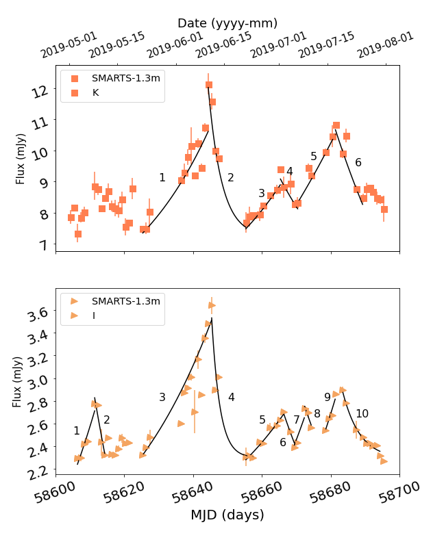
Figure 13: Flux light curves in $I$ and $K$ bands from SMARTS-1.3m. Each of the segments are fitted by a power law to estimate the doubling/halving time that can be found in Table 10.

Table 10: Doubling/halving times, $t_{d}$, in the K and I filters. The segments correspond to those in Figure 13.

Filter	Segment	$t_{d}$ (days)
K	1	28.1
K	2	6.7
K	3	31.8
K	4	25.6
K	5	34.2
K	6	21.6
I	1	18.2
I	2	12.2
I	3	28.7
I	4	7.7
I	5	35.6
I	6	20.7
I	7	21.5
I	8	20.9
I	9	19.7
I	10	13.6

References

- Abdo et al. (2009) Abdo A. A., et al., 2009, ApJS, 183, 46
- Abdo et al. (2010) Abdo A. A., et al., 2010, ApJ, 716, 30
- Abdo et al. (2011) Abdo A. A., et al., 2011, ApJ, 733, L26
- Abdollahi et al. (2020) Abdollahi S., et al., 2020, ApJS, 247, 33
- Abdollahi et al. (2022) Abdollahi S., et al., 2022, ApJS, 260, 53
- Abe et al. (2022) Abe H., et al., 2022, arXiv e-prints, p. arXiv:2210.02547
- Abhir et al. (2021) Abhir J., Joseph J., Patel S. R., Bose D., 2021, MNRAS, 501, 2504
- Ajello et al. (2020) Ajello M., et al., 2020, ApJ, 892, 105
- Alexander (1997) Alexander T., 1997, in Maoz D., Sternberg A., Leibowitz E. M., eds, Astrophysics and Space Science Library Vol. 218, Astronomical Time Series. p. 163, doi:10.1007/978-94-015-8941-3_14
- Amaya-Almazán et al. (2022) Amaya-Almazán R. A., Chavushyan V., Patiño Álvarez V. M., 2022, arXiv e-prints, p. arXiv:2202.08987
- Andernach et al. (2021) Andernach H., Jiménez-Andrade E. F., Willis A. G., 2021, Galaxies, 9, 99
- Asmus et al. (2015) Asmus D., Gandhi P., Hönig S. F., Smette A., Duschl W. J., 2015, MNRAS, 454, 766
- Astropy Collaboration et al. (2013) Astropy Collaboration et al., 2013, A&A, 558, A33
- Astropy Collaboration et al. (2018) Astropy Collaboration et al., 2018, AJ, 156, 123
- Bassani et al. (2016) Bassani L., Venturi T., Molina M., Malizia A., Dallacasa D., Panessa F., Bazzano A., Ubertini P., 2016, MNRAS, 461, 3165
- Bellm et al. (2019) Bellm E. C., et al., 2019, PASP, 131, 018002
- Bhukta et al. (2022) Bhukta N., Pal S., Mondal S. K., 2022, MNRAS, 512, 4308
- Blandford & Königl (1979) Blandford R. D., Königl A., 1979, ApJ, 232, 34
- Blandford & Rees (1978) Blandford R. D., Rees M. J., 1978, Phys. Scr., 17, 265
- Bonning et al. (2012) Bonning E., et al., 2012, ApJ, 756, 13
- Böttcher et al. (2013) Böttcher M., Reimer A., Sweeney K., Prakash A., 2013, ApJ, 768, 54
- Brown (2013) Brown A. M., 2013, MNRAS, 431, 824
- Bruni et al. (2020) Bruni G., et al., 2020, MNRAS, 494, 902
- Burrows et al. (2005) Burrows D. N., et al., 2005, Space Sci. Rev., 120, 165
- Chavushyan et al. (2020) Chavushyan V., Patiño-Álvarez V. M., Amaya-Almazán R. A., Carrasco L., 2020, ApJ, 891, 68
- Cleary et al. (2007) Cleary K., Lawrence C., Marshall J., Hao L., Meier D., 2007, ApJ, 660, 117
- Crossley et al. (2007) Crossley J. H., Sjouwerman L. O., Fomalont E. B., Radziwill N. M., 2007, in American Astronomical Society Meeting Abstracts. p. 132.03
- D’Abrusco et al. (2014) D’Abrusco R., Massaro F., Paggi A., Smith H. A., Masetti N., Landoni M., Tosti G., 2014, ApJS, 215, 14
- Dembinski & et al. (2020) Dembinski H., et al. P. O., 2020, ] 10.5281/zenodo.3949207
- Dennett-Thorpe et al. (2002) Dennett-Thorpe J., Scheuer P. A. G., Laing R. A., Bridle A. H., Pooley G. G., Reich W., 2002, MNRAS, 330, 609
- Dermer & Giebels (2016) Dermer C. D., Giebels B., 2016, Comptes Rendus Physique, 17, 594
- Dermer & Schlickeiser (1993) Dermer C. D., Schlickeiser R., 1993, ApJ, 416, 458
- Dickey & Lockman (1990) Dickey J. M., Lockman F. J., 1990, ARA&A, 28, 215
- Edelson & Krolik (1988) Edelson R. A., Krolik J. H., 1988, ApJ, 333, 646
- Emmanoulopoulos et al. (2013) Emmanoulopoulos D., McHardy I. M., Papadakis I. E., 2013, MNRAS, 433, 907
- Fernandes et al. (2020) Fernandes S., Patiño-Álvarez V. M., Chavushyan V., Schlegel E. M., Valdés J. R., 2020, MNRAS, 497, 2066
- Flesch (2015) Flesch E. W., 2015, Publ. Astron. Soc. Australia, 32, e010
- Flesch (2019) Flesch E. W., 2019, arXiv e-prints, p. arXiv:1912.05614
- Förster et al. (2021) Förster F., et al., 2021, AJ, 161, 242
- Fraija et al. (2019) Fraija N., Benítez E., Hiriart D., Sorcia M., López J. M., Mújica R., Cabrera J. I., Galván-Gámez A., 2019, ApJS, 245, 18
- Frank et al. (2002) Frank J., King A., Raine D. J., 2002, Accretion Power in Astrophysics: Third Edition
- Gaskell & Sparke (1986) Gaskell C. M., Sparke L. S., 1986, ApJ, 305, 175
- Ghisellini et al. (2005) Ghisellini G., Tavecchio F., Chiaberge M., 2005, A&A, 432, 401
- Giommi et al. (2012a) Giommi P., Padovani P., Polenta G., Turriziani S., D’Elia V., Piranomonte S., 2012a, MNRAS, 420, 2899
- Giommi et al. (2012b) Giommi P., et al., 2012b, A&A, 541, A160
- Gopal-Krishna et al. (2012) Gopal-Krishna Biermann P. L., Gergely L. Á., Wiita P. J., 2012, Research in Astronomy and Astrophysics, 12, 127
- Graham et al. (2019) Graham M. J., et al., 2019, PASP, 131, 078001
- Guise et al. (2022) Guise E., et al., 2022, MNRAS, 510, 3145
- Hernández-García et al. (2013) Hernández-García L., González-Martín O., Márquez I., Masegosa J., 2013, A&A, 556, A47
- Hernández-García et al. (2017) Hernández-García L., et al., 2017, A&A, 603, A131
- Hernández-García et al. (2018) Hernández-García L., et al., 2018, MNRAS, 478, 4634
- Hickox et al. (2014) Hickox R. C., Mullaney J. R., Alexander D. M., Chen C.-T. J., Civano F. M., Goulding A. D., Hainline K. N., 2014, ApJ, 782, 9
- Ishwara-Chandra & Saikia (1999) Ishwara-Chandra C. H., Saikia D. J., 1999, MNRAS, 309, 100
- Joshi et al. (2019) Joshi R., et al., 2019, ApJ, 887, 266
- Kapanadze et al. (2018) Kapanadze B., Vercellone S., Romano P., Hughes P., Aller M., Aller H., Kharshiladze O., Tabagari L., 2018, ApJ, 858, 68
- Kaspi et al. (2007) Kaspi S., Brandt W. N., Maoz D., Netzer H., Schneider D. P., Shemmer O., 2007, ApJ, 659, 997
- Kataoka et al. (2001) Kataoka J., et al., 2001, ApJ, 560, 659
- Kelly et al. (2009) Kelly B. C., Bechtold J., Siemiginowska A., 2009, ApJ, 698, 895
- Konar et al. (2006) Konar C., Saikia D. J., Jamrozy M., Machalski J., 2006, MNRAS, 372, 693
- Koshida et al. (2014) Koshida S., et al., 2014, ApJ, 788, 159
- Lacy et al. (2020) Lacy M., et al., 2020, PASP, 132, 035001
- Langejahn et al. (2020) Langejahn M., et al., 2020, A&A, 637, A55
- Lara et al. (1999) Lara L., Márquez I., Cotton W. D., Feretti L., Giovannini G., Marcaide J. M., Venturi T., 1999, A&A, 348, 699
- Lara et al. (2001) Lara L., Cotton W. D., Feretti L., Giovannini G., Marcaide J. M., Márquez I., Venturi T., 2001, A&A, 370, 409
- Lara et al. (2002) Lara L., Giovannini G., Cotton W. D., Feretti L., Marcaide J. M., Márquez I., Taylor G. B., Venturi T., 2002, New Astron. Rev., 46, 89
- Leahy & Parma (1992) Leahy J. P., Parma P., 1992, in Roland J., Sol H., Pelletier G., eds, Extragalactic Radio Sources. From Beams to Jets. pp 307–308
- Leahy & Williams (1984) Leahy J. P., Williams A. G., 1984, MNRAS, 210, 929
- Lira et al. (2015) Lira P., Arévalo P., Uttley P., McHardy I. M. M., Videla L., 2015, MNRAS, 454, 368
- MAGIC Collaboration et al. (2018) MAGIC Collaboration et al., 2018, A&A, 619, A45
- MacLeod et al. (2011) MacLeod C. L., et al., 2011, ApJ, 728, 26
- Machalski et al. (2016) Machalski J., Jamrozy M., Stawarz Ł., Weżgowiec M., 2016, A&A, 595, A46
- Marconi et al. (2004) Marconi A., Risaliti G., Gilli R., Hunt L. K., Maiolino R., Salvati M., 2004, MNRAS, 351, 169
- Masci et al. (2019) Masci F. J., et al., 2019, PASP, 131, 018003
- Massaro et al. (2015) Massaro E., Maselli A., Leto C., Marchegiani P., Perri M., Giommi P., Piranomonte S., 2015, Ap&SS, 357, 75
- McConnell et al. (2020) McConnell D., et al., 2020, Publications of the Astronomical Society of Australia, 37, e048
- Minezaki et al. (2019) Minezaki T., et al., 2019, ApJ, 886, 150
- Mishra et al. (2021) Mishra H. D., et al., 2021, ApJ, 913, 146
- Monet et al. (2003) Monet D. G., et al., 2003, AJ, 125, 984
- Netzer (2013) Netzer H., 2013, The Physics and Evolution of Active Galactic Nuclei
- Nordin et al. (2018) Nordin J., Brinnel V., Giomi M., Gal-yam A., Yaron O., Schulze S., 2018, Transient Name Server Discovery Report, 2018-1749, 1
- Oh et al. (2015) Oh K., Yi S. K., Schawinski K., Koss M., Trakhtenbrot B., Soto K., 2015, ApJS, 219, 1
- Ojha et al. (2004) Ojha R., et al., 2004, AJ, 127, 3609
- Ott et al. (1994) Ott M., Witzel A., Quirrenbach A., Krichbaum T. P., Standke K. J., Schalinski C. J., Hummel C. A., 1994, A&A, 284, 331
- Padovani et al. (2017) Padovani P., et al., 2017, A&ARv, 25, 2
- Pajdosz-Śmierciak et al. (2018) Pajdosz-Śmierciak U., Jamrozy M., Soida M., Stawarz Ł., 2018, ApJ, 868, 64
- Pajdosz-Śmierciak et al. (2022) Pajdosz-Śmierciak U., Śmierciak B., Jamrozy M., 2022, MNRAS, 514, 2122
- Pandey & Stalin (2022) Pandey A., Stalin C. S., 2022, A&A, 668, A152
- Panessa et al. (2016) Panessa F., et al., 2016, MNRAS, 461, 3153
- Patiño-Álvarez et al. (2018) Patiño-Álvarez V. M., et al., 2018, MNRAS, 479, 2037
- Pei et al. (2022) Pei Z., Fan J., Yang J., Huang D., Li Z., 2022, ApJ, 925, 97
- Priya et al. (2022) Priya S., Prince R., Agarwal A., Bose D., Özdönmez A., Ege E., 2022, MNRAS, 513, 2239
- Rees (1984) Rees M. J., 1984, ARA&A, 22, 471
- Roming et al. (2005) Roming P. W. A., et al., 2005, Space Sci. Rev., 120, 95
- Ruan et al. (2012) Ruan J. J., et al., 2012, ApJ, 760, 51
- Sahakyan et al. (2020) Sahakyan N., Harutyunyan G., Israelyan D., Khachatryan M., 2020, Astrophysics, 63, 334
- Saikia & Jamrozy (2009) Saikia D. J., Jamrozy M., 2009, Bulletin of the Astronomical Society of India, 37, 63
- Saito et al. (2013) Saito S., Stawarz Ł., Tanaka Y. T., Takahashi T., Madejski G., D’Ammando F., 2013, ApJ, 766, L11
- Sánchez-Sáez et al. (2018) Sánchez-Sáez P., Lira P., Mejía-Restrepo J., Ho L. C., Arévalo P., Kim M., Cartier R., Coppi P., 2018, ApJ, 864, 87
- Sánchez-Sáez et al. (2021) Sánchez-Sáez P., et al., 2021, AJ, 161, 141
- Sánchez et al. (2017) Sánchez P., et al., 2017, ApJ, 849, 110
- Schawinski et al. (2015) Schawinski K., Koss M., Berney S., Sartori L. F., 2015, MNRAS, 451, 2517
- Shen (2021) Shen Y., 2021, ApJ, 921, 70
- Stassun et al. (2019) Stassun K. G., et al., 2019, AJ, 158, 138
- Tonry et al. (2018) Tonry J. L., et al., 2018, PASP, 130, 064505
- Tramacere (2020) Tramacere A., 2020, JetSeT: Numerical modeling and SED fitting tool for relativistic jets, Astrophysics Source Code Library, record ascl:2009.001 (ascl:2009.001)
- Tramacere et al. (2009) Tramacere A., Giommi P., Perri M., Verrecchia F., Tosti G., 2009, A&A, 501, 879
- Tramacere et al. (2011) Tramacere A., Massaro E., Taylor A. M., 2011, ApJ, 739, 66
- Urry & Padovani (1995) Urry C. M., Padovani P., 1995, PASP, 107, 803
- Vaughan et al. (2003) Vaughan S., Edelson R., Warwick R. S., Uttley P., 2003, MNRAS, 345, 1271
- Zargaryan et al. (2022) Zargaryan D., Mackey J., Barnouin T., Aharonian F., 2022, MNRAS, 510, 1118
- Zhu et al. (2018) Zhu S. F., Xue Y. Q., Brandt W. N., Cui W., Wang Y. J., 2018, ApJ, 853, 34