Surviving the Waves: evidence for a Dark Matter cusp in the tidally disrupting Small Magellanic Cloud

Abstract

We use spectroscopic data for ${\sim}6,000$ Red Giant Branch (RGB) stars in the Small Magellanic Cloud (SMC), together with proper motion data from Gaia Early Data Release 3 (EDR3), to build a mass model of the SMC. We test our Jeans mass modelling method (Binulator+GravSphere) on mock data for an SMC-like dwarf undergoing severe tidal disruption, showing that we are able to successfully remove tidally unbound interlopers, recovering the Dark Matter density and stellar velocity anisotropy profiles within our 95% confidence intervals. We then apply our method to real SMC data, finding that the stars of the cleaned sample are isotropic at all radii (at 95% confidence), and that the inner Dark Matter density profile is dense, $\rho_{\rm DM}(150\,{\rm pc})=2.81_{-1.07}^{+0.72}\times 10^{8}M_{\odot}\rm kpc^{-3}$, consistent with a $\Lambda$ Cold Dark Matter ($\Lambda$CDM) cusp at least down to 400 pc from the SMC’s centre. Our model gives a new estimate of the SMC’s total mass within 3 kpc ($M_{\rm tot}\leq 3\,{\rm kpc})$ of $2.34\pm 0.46\times 10^{9}M_{\odot}$. We also derive an astrophysical “$J$-factor” of $19.22\pm 0.14$  GeV² cm^-5 and a “$D$-factor” of $18.80\pm 0.03$  GeV² cm^-5, making the SMC a promising target for Dark Matter annihilation and decay searches. Finally, we combine our findings with literature measurements to test models in which Dark Matter is “heated up” by baryonic effects. We find good qualitative agreement with the Di Cintio et al. 2014 model but we deviate from the Lazar et al. 2020 model at high $M_{*}/M_{200}>10^{-2}$. We provide a new, analytic, density profile that reproduces Dark Matter heating behaviour over the range $10^{-5}<M_{*}/M_{200}<10^{-1}$.

1 Introduction

One of the long-standing problems of the prevailing $\Lambda$ Cold Dark Matter ($\Lambda$CDM) cosmological model is the discrepancy between the observed constant density “cores” of gas rich dwarf galaxies ($\rho_{DM}(150\,{\rm pc})\sim$ constant $\sim 5\times 10^{7}$ M_⊙ kpc^-3; e.g. Moore 1994; Flores & Primack 1994; Read et al. 2017) and the dense “cusps” predicted by pure Dark Matter structure formation simulations ($\rho_{DM}(150\,{\rm pc})>10^{8}$ M_⊙ kpc^-3; e.g. Dubinski & Carlberg 1991; Navarro et al. 1996b, 1997). Numerous solutions to this so-called “cusp-core problem” have been proposed, falling into three main categories. The first class of solution proposes new Dark Matter models, such as Self Interacting Dark Matter (Spergel & Steinhardt, 2000), Warm Dark Matter (e.g. Hogan & Dalcanton, 2000; Bode et al., 2001; Avila-Reese et al., 2001), or “Wave-like” Dark Matter (e.g. Schive et al., 2014). The second class challenges the interpretation of the data in some cases, for example the existence of systematic errors due to the typically assumed spherical symmetry and circular gas motions (e.g. Read et al., 2016b; Genina et al., 2018; Oman et al., 2019). The third class proposes that “baryonic effects”, like repeated gas cooling and blowout through the starburst cycle, can kinematically “heat” the Dark Matter pushing it out of the centres of dwarf galaxies (e.g. Navarro et al., 1996a; Gnedin & Zhao, 2002; El-Zant et al., 2001; Read & Gilmore, 2005; Mashchenko et al., 2008; Pontzen & Governato, 2012; Di Cintio et al., 2014a; Di Cintio et al., 2014b; Pontzen & Governato, 2014; Orkney et al., 2021). This third class of solution has been gaining traction due to it making a number of testable predictions that are now supported by a host of observational data. Dark Matter heating models predict that star formation should be bursty, with a peak-to-trough burst amplitude of $\sim$10, a burst duration shorter than the local dynamical time and a kinematically “hot” stellar disc (e.g. Teyssier et al., 2013; Sparre et al., 2017). The same models predict that stars should slowly migrate outwards (Read & Gilmore, 2005), yielding an age gradient (e.g. El-Badry et al., 2016) and that cusp-core transformations need to take many dynamical times, meaning that dwarf galaxies with truncated star formation should be more cuspy than those with extended star formation (e.g. Di Cintio et al., 2014a; Read et al., 2016a). All of these predictions have been borne out by data so far (e.g. Kauffmann, 2014; Leaman et al., 2012; Emami et al., 2019; Zhang et al., 2012; Read et al., 2019; Collins & Read, 2022).

However, a key forecast of Dark Matter heating models has only recently been tested. Following Peñarrubia et al. (2012), Di Cintio et al. (2014a) parameterise the amount of cusp-core transformation a dwarf galaxy undergoes by its stellar-to-halo mass ratio, $M_{*}/M_{200}$. This works to leading order because $M_{*}$ is proportional to the total integrated supernova energy available to unbind the Dark Matter cusp, while $M_{200}$ represents the potential well depth and, therefore, how much energy is required. Di Cintio et al. (2014a) predict cusped dwarfs for $M_{*}/M_{200}\lesssim 5\times 10^{-4}$, cored dwarfs for $5\times 10^{-4}\lesssim M_{*}/M_{200}\lesssim 5\times 10^{-2}$, and cusped dwarfs again for $M_{*}/M_{200}\gtrsim 10^{-2}$, with this latter owing to the potential well depth winning over the energy available to unbind the cusp. Read et al. (2019) measured the inner Dark Matter densities of 16 nearby dwarfs with $10^{-4}\lesssim M_{*}/M_{200}\lesssim 5\times 10^{-3}$, finding excellent qualitative agreement with Di Cintio et al. (2014a). In a similar study, Bouché et al. (2022) probed $10^{-3}\lesssim M_{*}/M_{200}\lesssim 3\times 10^{-2}$, finding results consistent with Read et al. (2019) where they overlap, and favouring a return cuspy galaxies at higher $M_{*}/M_{200}$, as predicted by Di Cintio et al. (2014a). However, Bouché et al. (2022) base their study on dwarfs at a redshift $z=1$ that are not necessarily comparable with the local sample from Read et al. (2019). In this context, the Small Magellanic Cloud (SMC), with $M_{*}/M_{200}\sim 7\times 10^{-3}$, and at a distance of $\sim 62\pm 1.28$ kpc (Graczyk et al., 2020) from us poses a unique opportunity to test Dark Matter heating models at a higher $M_{*}/M_{200}$ than previously probed for nearby dwarfs. The main challenge to using a standard equilibrium mass modelling method in this galaxy is the overwhelming evidence showing that the outskirts of the SMC are in fact tidally disrupted (e.g. Evans & Howarth 2008; Olsen et al. 2011; Noël et al. 2013; Ripepi et al. 2014; Dobbie et al. 2014; Noël et al. 2015; Carrera et al. 2017;Zivick et al. 2018, 2019; Massana et al. 2020; De Leo et al. 2020; Zivick et al. 2021; Niederhofer et al. 2021). The hypothesis of heavy tidal disruption is also supported by the observations of distance-tracer populations such as classical Cepheids (i.e. Jacyszyn-Dobrzeniecka et al., 2016; Scowcroft et al., 2016; Ripepi et al., 2017) and RR Lyrae (i.e. Jacyszyn-Dobrzeniecka et al., 2017; Muraveva et al., 2018) that show a long line-of-sight depth for the SMC.

Fortunately, there is no direct observational evidence that the tidal disruption extends to the inner regions of the SMC. It is thus possible to reconcile the observations of extended disruption and long line-of-sight depth previously mentioned with equilibrium mass modelling by hypothesising that the SMC is composed of a bound remnant surrounded by an extended field of tidal debris. The key to successfully model the galaxy’s remnant then resides in the removal of the debris.

In this paper, we combine the unprecedented kinematic sample of ${\sim}6000$ SMC stars from De Leo et al. (2020), that includes line of sight velocities and proper motions, with the Jeans modeling code GravSphere (Read & Steger, 2017; Read et al., 2018; Genina et al., 2020; Collins et al., 2021) to produce a new mass model of the SMC. We assume that the SMC’s tidal disruption is not complete, such that the central bound region of the galaxy can be modelled assuming pseudo-dynamic equilibrium. We use a new binning module for GravSphere called the binulator (Collins et al., 2021) to successfully remove tidally unbound stars. To test these key assumptions, we apply our method to mock data for a severely disrupting SMC, showing that even in this extreme case, we are able to correctly infer the stellar velocity anisotropy and inner Dark Matter density within our 95% confidence intervals. We use our new dynamical model to test Dark Matter heating models and constrain the pre-infall mass of the SMC. We discuss whether the SMC is a promising target for Dark Matter annihilation and/or decay searches (e.g. Caputo et al., 2016).

This paper is organised as follows. In §2, we present the data used for the mass model. In §3, we discuss the GravSphere+binulator mass modelling method. In §4, we present our results which we discuss in §5. Finally, we present our conclusions in §6.

2 Data

In this section, we describe both the observational (§2.1) and simulation data (§2.2) that we use to generate the mock data for this study.

2.1 Observational data

We used spectroscopic data of RGB stars in the SMC area from the catalogues presented in De Leo et al. (2020) and Dobbie et al. (2014), the Gaia DR2 Gaia Collaboration et al. (2018) and EDR3 Gaia Collaboration et al. (2021) catalogues, and a photometric selection of RGB stars from the Survey of the MAgellanic Stellar History (SMASH, Nidever et al., 2021), cross-matched with Gaia EDR3.

2.1.1 Radial velocities

We used the radial velocity determinations from the “extended” sample presented in De Leo et al. (2020) which also includes SMC RGB stars from Dobbie et al. (2014). For the full details of the analysis that led to the radial velocity determinations see De Leo et al. (2020). Briefly, the raw spectra acquired with the 2dF+AAOmega instrument at the AAT were processed with the 2dfdr tool (Sharp & Birchall, 2010) and proprietary software to reduce them, remove sky contamination, subtract the solar reflex motion and finally derive radial velocities through cross-correlation with a grid of synthetic spectra (details of the grid in Allende Prieto et al. 2018). This sample includes $\sim 6000$ RGB stars which are confirmed SMC members (i.e. with radial velocities $V_{r}$ between 70 and 230 km s^-1). The distribution of radial velocities can be seen on the left panel of Fig. 1 where the large velocity dispersion of the system (c.f. Hatzidimitriou et al., 1993; Harris & Zaritsky, 2006) is clearly appreciated.

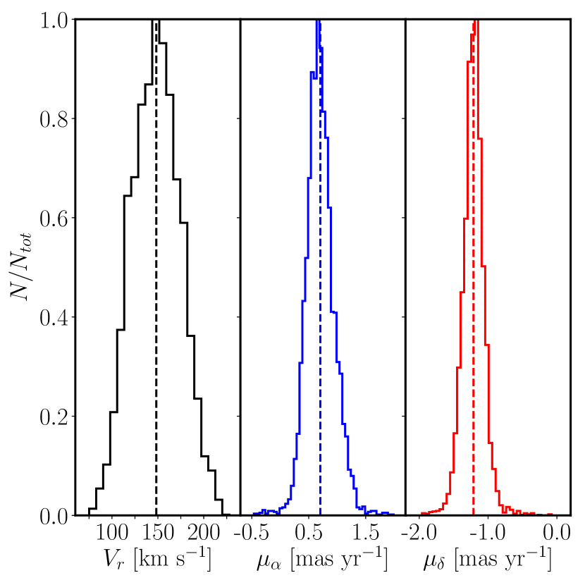
Figure 1: Kinematic distributions of our sample stars. Each panel shows an histogram that represents the distribution of one of the velocity components; the perpendicular dashed lines represent the mean values. The velocity components shown are the radial velocity $V_{r}$ (in black in the left panel), the proper motion $\mu_{\alpha}$ (in blue in the middle panel), and the proper motion $\mu_{\delta}$ (in red in the right panel).

2.1.2 Proper motions

We cross-matched the radial velocity sample presented above with the Gaia EDR3 catalogue. For discussions on the systematics of Gaia see Lindegren et al. (2018), the recommendations from L. Lindegren and Lindegren et al. (2021). The total error budget for the proper motions in Gaia is as follows:

$$\sigma_{tot}=\sqrt{k^{2}\sigma_{i}^{2}+\sigma_{s}^{2}}$$ (1)

where $k$ is a factor accounting for the underestimation of the observational uncertainties, $\sigma_{i}$ is the measured uncertainty for the i-th star and $\sigma_{s}$ is the systematic error. The main difference with the data presented in De Leo et al. (2020) (which used proper motions from Gaia DR2) is in the lower observational uncertainties and systematics of Gaia EDR3 which translated into an improvement of about 65% in the systematic error $\sigma_{s}$ and total uncertainties which are on average 47% and 35% smaller, respectively for $\mu_{\alpha}\cos{\delta}$ and $\mu_{\delta}$. Throughout the paper we will refer to the proper motion $\mu_{\alpha}\cos{\delta}$ simply as $\mu_{\alpha}$. The distributions of proper motions can be seen in blue ($\mu_{\alpha}$) and in red ($\mu_{\delta}$) respectively in the middle and right panels of Fig. 1. Both distributions show long tails and the distribution of $\mu_{\alpha}$ (the blue histogram in the middle panel) shows larger dispersion and asymmetry favouring proper motions higher than the mean.

2.1.3 Stellar surface density

The kinematic sample presented above (radial velocities plus proper motions) was too small and incomplete to provide a reliable estimation of the stellar surface density. To have a more complete sampling of the inner regions of the SMC we derived the stellar surface density from a selection of RGB stars from SMASH, crossmatched with Gaia EDR3. Using the deep photometry of SMASH and proper motions and parallaxes from Gaia EDR3 for foreground decontamination, we produced an accurate density profile of upper RGB bona-fide SMC candidates out to $\sim$11^∘ from the centre of the galaxy (that for this sample is at $\alpha_{c}$, $\delta_{c}$ = 13.16^∘, -72.80^∘). The density is computed first counting the number of stars in each HEALPix (Górski et al., 2005; Zonca et al., 2019) pixel (nside=512), then dividing the SMC projected surface in equal-radius (0$\aas@@fstack{\circ}$3) annuli centred on ($\alpha_{c}$, $\delta_{c}$) and averaging the number of stars over the pixels included in each given annulus (taking into account that all pixels have equal area). Given the large number of RGB stars present in the SMASH sample, we were able to compute statistical uncertainties on the average values by taking the standard deviations in each annulus. This provided an accurate stellar surface density profile based on the same type of stars of our kinematics tracers and useful over large radii (see Figure 2).

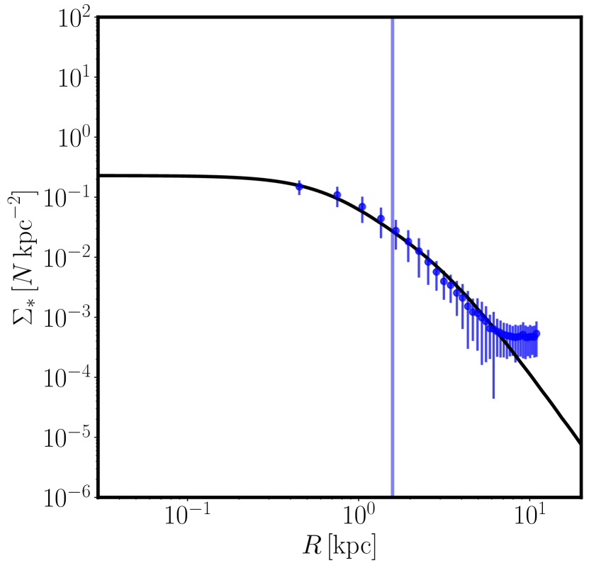
Figure 2: Surface number density profile, $\Sigma_{*}(r)$, of the SMASH sample of RGB stars cross-matched with Gaia EDR3. The black line is the best fit model from GravSphere, the blue points with 68% confidence intervals are the profile computed from real data, and the fainter blue vertical line is the half-light radius computed by GravSphere.

2.2 Simulation data

In order to test our analysis method and mass model, we used two SMC-analogues taken from the suite of simulations presented in De Leo et al. (2020). One is a “bound” SMC that has undergone little tidal stripping. The other is a “heavily disrupted” SMC that is close to full dissolution. This latter is closest to the real SMC data though is likely more extreme. In particular, it starts out close to the SMC’s current inner velocity dispersion before tidal stripping and shocking. As such, its final inner velocity dispersion is substantially colder than the true SMC data. This is nonetheless perfectly acceptable for testing our methodology.

The simulation set-up is described in detail in De Leo et al. (2020). Here, we briefly summarise the key points. We ran a grid of $N$-body simulations using gadget-3 (an updated version of gadget-2; Springel, 2005) with a live SMC ($10^{5}$ particles, a total mass of $M_{\rm SMC}=10^{9}M_{\odot}$, and two different scale radii, as outlined below) modelled as a Plummer sphere (Plummer, 1911) disrupting around a $1.5\times 10^{11}\,{\rm M}_{\odot}$ LMC (Erkal et al., 2019) in the presence of the Milky Way (modelled using the MWPotential2014 model from Bovy 2015). As specified in the original paper, the initial mass used for the SMC is based on its present-day dynamical mass (i.e., Harris & Zaritsky, 2006), substantially lower than its likely peak mass before infall ($\sim 5\times 10^{10}\,{\rm M}_{\odot}$; Read & Erkal 2019). This is motivated by the fact that the simulations were not meant to faithfully model the entire disruption history of the SMC but only its final phases, once the SMC had lost the majority of its Dark Matter (Smith et al., 2016). The two simulations selected for the analysis in this work are at the opposite ends of the spectrum of explored scale radii, the most bound (0.8 kpc initial scale radius) and the most disrupted (1.5 kpc initial scale radius) SMC-analogues. The former bound SMC is used to test that the method works properly and is able to recover the true density profile in the absence of disrupting influences; the latter heavily disrupted SMC is the closest analogue to our observed case and likely, in fact, more extreme (see Figure 3 for a visual representation).

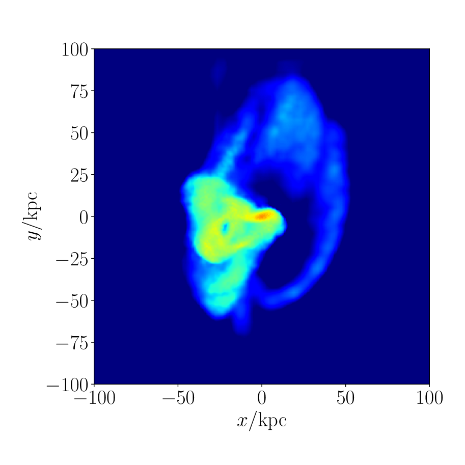
Figure 3: Density map of the heavily disrupted simulation (De Leo et al., 2020)) projected on the $XY$-plane of the simulation phase space and centred on its photometric centre. Blue pixels have no particles in them. The density increases from cyan to light green, yellow and orange for the densest regions in the centre. The cyan and light green plumes and arcs trace the past orbit of the simulated galaxy and are composed of particles making up tidal debris around the central bound remnant of the galaxy.

Both the observed and the simulation data were treated with the same analysis pipeline and mass modeling tool. This procedure included adding errors for the simulation data resembling the observational ones. The errors for the simulation data were sampled from Gaussians for each observable ($V_{r}$, $\mu_{\alpha}$ or $\mu_{\delta}$). The results of this procedure can be seen in Fig. 4, where in each panel the black histograms are the observed errors (left panel for $\rm{Err_{Vr}}$, middle panel for $\rm{Err_{\mu_{\alpha}}}$ and right panel for $\rm{Err_{\mu_{\delta}}}$) and the red dot-dashed lines are the Gaussians sampled to generate the simulation errors.

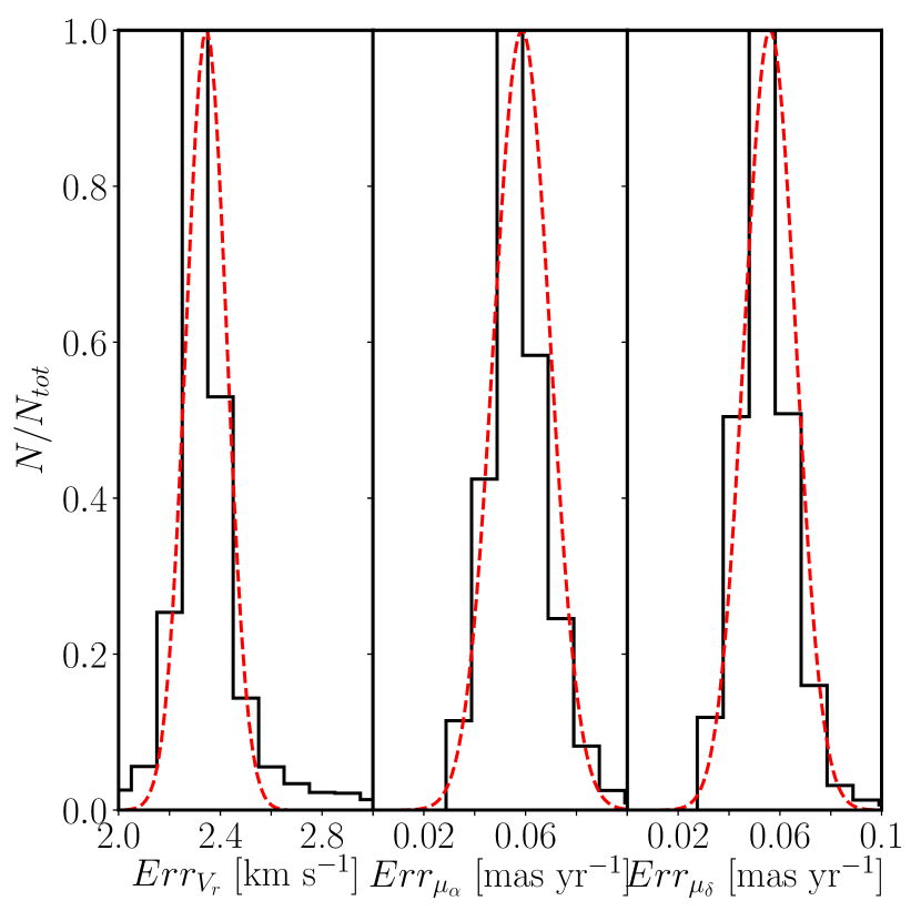
Figure 4: Distributions of the observed errors for the real SMC data (black histograms) and Gaussians from which the errors for the simulated mock SMC-analogues are sampled (red dash-dotted lines). Each panel shows a different variable: $V_{r}$ (left panel), $\mu_{\alpha}$ (middle panel), and $\mu_{\delta}$ (right panel).

Regarding the errors for the simulation data, it is important to keep in mind that, as pointed out in De Leo et al. (2020), the simulated SMC analogues are less massive than the real SMC, leading to kinematically cooler velocity dispersion profiles (see also the discussion, above). Thus, when drawing our errors from the real SMC observations, we overestimate the fractional uncertainty on the simulated dispersion profiles. This means that our mock data present a worst-case scenario for testing our analysis pipeline.

3 Mass Modelling

3.1 GravSphere

Our mass modelling technique is based on solving the spherical Jeans equation (e.g. Jeans, 1922; Binney, 1980; Binney & Tremaine, 2008):

$$\frac{1}{\nu}\frac{\partial}{\partial r}(\nu\sigma_{r}^{2})+\frac{2\beta(r)\sigma_{r}^{2}}{r}=-\frac{GM(<r)}{r^{2}}$$ (2)

where $\nu(r)$ is the kinematic tracer density; $\sigma_{r}^{2}=\langle v_{r}^{2}\rangle-{\langle v_{r}\rangle}^{2}$ is the velocity dispersion of the tracers; $G=6.67398\times 10^{-11}$ $\rm{m^{3}{kg}^{-1}s^{-2}}$ is Newton’s gravitational constant; $M(<r)$ is the total mass inside spherical radius $r$; and $\beta(r)=1-\sigma_{t}^{2}/\sigma_{r}^{2}$ is the velocity anisotropy, where $\sigma_{t}$ is the tangential velocity dispersion. This equation is valid under the assumptions of no rotation (which we excluded for the SMC RGB population in De Leo et al. 2020), dynamical equilibrium, and spherical symmetry. We will test these latter two assumptions with mock data in §2.2.

We solve equation 2 using the GravSphere code with the aim of recovering the total cumulative mass (stars and Dark Matter), the Dark Matter density profile $\rho_{DM}(r)$ and the stellar velocity anisotropy profile $\beta(r)$ of the object being studied. The full methodology is described and tested in detail in Read & Steger (2017); Read et al. (2018); Genina et al. (2020); Read et al. (2021); Collins et al. (2021). The code is publicly available and has already been used to model a wide range of nearby spherical stellar systems (e.g. Read et al., 2018, 2019; Collins et al., 2021; Zoutendijk et al., 2021a). Here, we briefly summarise the main points.

Eq. 2 is integrated along the line of sight to obtain expressions for the line of sight, radial and tangential velocity dispersions, as a function of projected distance, $R$ (e.g. Binney & Mamon 1982; van der Marel 1994; Mamon & Łokas 2005):

$$\sigma_{LOS}^{2}=\frac{2}{\Sigma_{*}(R)}\int_{R}^{\infty}\bigg{(}1-\beta(r)\frac{R^{2}}{r^{2}}\bigg{)}\frac{\nu(r)\sigma_{r}^{2}(r)r}{\sqrt{r^{2}-R^{2}}}\rm{d}r$$ (3)

$$\sigma_{POSr}^{2}=\frac{2}{\Sigma_{*}(R)}\int_{R}^{\infty}\bigg{(}1-\beta(r)+\beta(r)\frac{R^{2}}{r^{2}}\bigg{)}\frac{\nu(r)\sigma_{r}^{2}(r)r}{\sqrt{r^{2}-R^{2}}}\rm{d}r$$ (4)

$$\sigma_{POSt}^{2}=\frac{2}{\Sigma_{*}(R)}\int_{R}^{\infty}(1-\beta(r))\frac{\nu(r)\sigma_{r}^{2}(r)r}{\sqrt{r^{2}-R^{2}}}\rm{d}r$$ (5)

where $\sigma_{LOS}$, $\sigma_{POSr}$ and $\sigma_{POSt}$ are the tracers’ line of sight, projected radial and projected tangential velocity dispersions; $\Sigma_{*}(R)$ is the tracers’ surface density at the projected radius $R$; and

$$\sigma_{r}^{2}(r)=\frac{1}{\nu(r)g(r)}\int_{r}^{\infty}\frac{GM(\widetilde{r})\nu(\widetilde{r})}{{\widetilde{r}}^{2}}g(\widetilde{r})\rm{d}\widetilde{r}$$ (6)

with:

$$g(r)={\rm exp}\left(2\int\frac{\beta(r)}{r}{\rm d}r\right)$$ (7)

GravSphere has the possibility of additionally using two Virial Shape Parameters (VSP1 and VSP2) that constrain the global kurtosis of the stellar distribution, allowing the degeneracy between the cumulative mass and the velocity anisotropy, present if only line-of-sight velocity data are available, to be broken (e.g. Merrifield & Kent, 1990; Richardson & Fairbairn, 2014; Read & Steger, 2017). However, for the SMC we have excellent constraints on $\sigma_{LOS}$, $\sigma_{POSr}$ and $\sigma_{POSt}$ that also break this same degeneracy (e.g. Strigari et al., 2007; Read & Steger, 2017). A key challenge in measuring VSPs for the SMC is that they formally require an integral over the kurtosis to infinity. This means that the kurtosis needs to be reliably measured at large radii where it could be strongly impacted by tides (e.g. De Leo et al., 2020). For mildly disrupting dwarfs, Read et al. (2018) show that an unbiased estimate of the VSPs can still be obtained by extrapolating the kurtosis to large radii from constraints further in. Using a similar approach, we were able to recover VSP1 for both the mock and real SMC data, but VSP2 – that is more sensitive to data further out – was very poorly constrained and so we do not use it in this paper. In the end, even VSP1 produced no measurable impact on our models since much stronger constraining power comes from the proper motion data. As such, while we use VSP1 by default throughout, we note that switching it off produces no noticeable change in our derived models or their confidence intervals.

GravSphere has evolved significantly since its first tests in Read & Steger (2017) and Read et al. (2018). The version we used here is the one presented in Collins et al. (2021). The most important changes were put in place to counteract a small bias in the density beyond $\sim 4R_{1/2}$ (Read & Steger, 2017; Read et al., 2021), and biases introduced by the binning method in the presence of a small number of tracers or large velocity errors (Gregory et al., 2020; Zoutendijk et al., 2021b; Collins et al., 2021). These prompted the development of the Binulator as a separate code to handle the data binning, and a switch of the mass model from a “non-parametric” series of power laws centred on radial bins to the coreNFWtides profile (Read et al., 2018; Read & Erkal, 2019). The two profiles have been shown to yield constraints on the cumulative mass profile that are statistically consistent with one another (Alvarez et al., 2020). However, the coreNFWtides density profile, $\rho_{\rm cNFWt}(r)$, has the advantage of producing profiles that more easily connect to parameters of interest in cosmological models:

$$\rho_{\rm cNFWt}(r)=\left\{\begin{array}[]{ll}\rho_{\rm cNFW}&r<r_{t}\\ \rho_{\rm cNFW}(r_{t})\left(\frac{r}{r_{t}}\right)^{-\delta}&r>r_{t}\end{array}\right.$$ (8)

where $r_{t}$ sets the radius at which mass is tidally stripped from the galaxy, $\delta$ sets the logarithmic density slope beyond $r_{t}$; $\rho_{\rm cNFW}$ is given by:

$$\rho_{\rm cNFW}(r)=f^{n}\rho_{\rm NFW}+\frac{nf^{n-1}(1-f^{2})}{4\pi r^{2}r_{c}}M_{\rm NFW};$$ (9)

$$M_{\rm cNFW}(<r)=M_{\rm NFW}(<r)f^{n};$$ (10)

the function $f^{n}$ generates a shallower profile below a core-size parameter, $r_{c}$:

$$f^{n}=\left[\tanh\left(\frac{r}{r_{c}}\right)\right]^{n};$$ (11)

and $M_{\rm NFW}(<r)$ is the cumulative mass of the ‘Navarro, Frenk & White’ (NFW) profile (Navarro et al., 1996b):

$$M_{\rm NFW}(r)=M_{200}g_{c}\left[\ln\left(1+\frac{r}{r_{s}}\right)-\frac{r}{r_{s}}\left(1+\frac{r}{r_{s}}\right)^{-1}\right];$$ (12)

$$g_{c}=\frac{1}{{\rm log}\left(1+c_{200}\right)-\frac{c_{200}}{1+c_{200}}};$$ (13)

$$r_{200}=\left[\frac{3}{4}M_{200}\frac{1}{\pi\Delta\rho_{\rm crit}}\right]^{1/3};$$ (14)

where $c_{200}$ is the dimensionless concentration parameter; $\Delta=200$ is the over-density parameter; $\rho_{\rm crit}=136.05$ M_⊙ kpc^-3 (in a $\Lambda$CDM cosmology) is the critical density of the Universe at redshift $z=0$; $r_{200}$ is the virial radius at which the mean enclosed density is $\Delta\times\rho_{\rm crit}$; and $M_{200}$ is the virial mass – the mass within $r_{200}$.

In GravSphere, the cumulative mass profile $M(r)$ is given by the sum of the stellar mass profile $M_{*}(r)$, which is assumed to follow the tracer distribution with a flat prior on the total stellar mass $3.45<4.6M_{*}/(10^{8}M_{\odot})<5.75$ (McConnachie, 2012), and the coreNFWtides profile (equation 8) for the Dark Matter. Our priors on the model parameters are reported in the first six rows of Table 1.

		Simulation run		Observation run
	Parameter	Minimum	Maximum	Minimum	Maximum
1	$\rm{log_{10}}(M_{200})$	5.5	11.5	7.5	11.5
2	$c_{200}$	1.0	100.0	7.43	52.63
3	$\rm{log_{10}}(r_{c})$	0.01	100.0	0.01	10.0
4	$n$	-1.0	1.0	-1.0	1.0
5	$\rm{log_{10}}(r_{t})$	0.1	10.0	1.0	20.0
6	$\delta$	3.01	8.0	3.01	8.0
7	$M_{1,2,3}$	-100	100	-5	5
8	$a_{1,2,3}$	0.01	2.0	0.1	2.5
9	$\rm{log}(r_{0})$	-2.0	1.0	-2.0	0.0
10	$\eta$	1.0	3.0	1.0	3.0
11	$\beta_{0}$	-0.1	0.1	-0.3	0.3
12	$\beta_{\infty}$	-0.1	1.0	-0.3	1.0
13	$\mu_{\nu}$	-50	50	-50	50
14	$\alpha_{\nu}$	4.0	15.0	10	60.0
15	$\beta_{\nu}$	1.0	5.0	1.0	5.0
16	$A_{0}$	0.0001	1.0	0.0001	1.0
17	$\mu$	-150.0	150.0	-250.0	250.0
18	$\sigma$	15.0	150.0	60.0	150.0

Table 1: Bounds on the priors and parameters used by GravSphere and the Binulator. The first six rows are the bounds of the flat priors assumed for the mass profile. $M_{200}$ is in $M_{\odot}$, $c_{200}$, $n$ and $\delta$ are dimensionless, $r_{c}$ and $r_{t}$ are in kpc. Rows 7 and 8 are the priors of the Plummer spheres used to fit the tracers density, with the $M_{j}$ dimensionless (as the surface density data are normalised) and $a_{j}$ in kpc. Rows from 9 to 12 are the priors for the anisotropy profile parameters where $r_{0}$ is in kpc and $\eta$, $\beta_{0}$, and $\beta_{\infty}$ are dimensionless. Rows 13 to 15 are the bounds of the parameter space searched for the fit of the residual velocity distributions. Rows 16 to 18 are the parameters of the secondary Gaussian used to model the contaminants of the velocity distributions (a standard Gaussian of amplitude $A_{0}$, mean $\mu$, and dispersion $\sigma$).

.

The tracer density is given by a sum of a series of $N_{p}$ Plummer spheres (Plummer, 1911; Rojas-Niño et al., 2016):

$$\nu=\sum_{j}^{N_{p}}\frac{3M_{j}}{4\pi a_{j}^{3}}{\bigg{(}1+\frac{r^{2}}{a_{j}^{2}}\bigg{)}}^{-5/2}$$ (15)

where $M_{j}$ and $a_{j}$ are the mass and scale length of each individual component. $\Sigma_{*}(R)$ appears in Eqs. 3,  4, and  5 and has to be compared with the data. Eq. 15 makes $\Sigma_{*}(R)$ analytic:

$$\Sigma_{*}(R)=\sum_{j}^{N_{p}}\frac{M_{j}}{\pi a_{j}^{2}}{\big{(}1+\frac{R^{2}}{a_{j}^{2}}\big{)}}^{-2}$$ (16)

Typically, $N_{p}=3$ is enough to model the tracer density, especially since the masses are allowed to be negative (under a constraint that the total density at all radii remains positive; Rojas-Niño et al. 2016). Rows 7 and 8 of Table 1 report the parameter space that the code searched when fitting the tracer densities for the models. The Binulator does a first fit of the tracer density and then GravSphere searches for a new solution around the best-fit within a preset tolerance (here chosen to be $10^{-3}$, as the data are very constraining).

The velocity anisotropy profile follows Baes & van Hese (2007) and Read & Steger (2017):

$$\beta(r)=\beta_{0}+(\beta_{\infty}-\beta_{0})\frac{1}{1+{(\frac{r_{0}}{r})}^{\eta}}$$ (17)

where $\beta_{0}$ is the anistotropy at the centre, $\beta_{\infty}$ is the value at infinity, $r_{0}$ is the transition radius, $\eta$ dictates the steepness of the profile and the priors for all the parameters are given in rows 9 to 12 of Table 1. This definition of anistropy allows for a wide range of anisotropy profiles while making Eq. 7 analytic. Even more general analytic forms are discussed and presented in Read & Steger 2017.

$\beta(r)$, as defined above, has values over an infinite range ($-\infty<\beta<1$) which is problematic for model fitting and, hence, GravSphere uses instead a symmetrised version (Read et al., 2006):

$$\widetilde{\beta}=\frac{\sigma_{r}^{2}-\sigma_{t}^{2}}{\sigma_{r}^{2}+\sigma_{t}^{2}}=\frac{\beta}{2-\beta}$$ (18)

With this definition, the anisotropy is bounded on a finite parameter space: $\widetilde{\beta}=1$ is full radial anisotropy, $\widetilde{\beta}=0$ is isotropy and $\widetilde{\beta}=-1$ is full tangential anisotropy.

GravSphere fits the tracers’ surface density (Eq. 16) and velocity dispersion profiles (Eq. 3, Eqs. 4 and  5) using the MCMC code Emcee (Foreman-Mackey et al., 2013). These fits allow for the reconstruction of the Dark Matter density and stellar velocity anistropy profiles through the other equations presented here.

3.2 The Binulator

In Collins et al. (2021), the binning routines of GravSphere were redeveloped and built into their own code, the Binulator. This implements one main change: each projected radial bin (that contains an equal number of stars, weighted by their membership probability) is fit with a generalised Gaussian, convolved with the error PDF of each star:

$$p_{i}=\frac{\beta_{\nu}}{2\tilde{\alpha}_{\nu}\Gamma(1.0/\beta_{\nu})}\rm{exp}\bigg{(}-{\frac{|\nu_{i}-\mu_{\nu}|}{\tilde{\alpha}_{\nu}}}^{\beta_{\nu}}\bigg{)}$$ (19)

where:

$$\widetilde{\alpha}^{2}=\alpha_{\nu}^{2}+\sigma_{e,i}^{2}\frac{\Gamma(1.0/\beta_{\nu})}{\Gamma(3.0/\beta_{\nu})}$$ (20)

and $\sigma_{e,i}$ is the width of the PDF of the error on the $i$-th star; $\nu_{i}$ is the velocity (be it line-of-sight or along one of the plane of the sky directions) of the $i$-th star; $\Gamma$(x) is the Gamma Function; and $\mu_{\nu}$, $\alpha_{\nu}$ and $\beta_{\nu}$ are parameters fit to each bin. These allow us to recover the mean, $\mu_{\nu}$, variance, $\sigma_{\nu}^{2}=\alpha_{\nu}^{2}\Gamma(3.0/\beta_{\nu})/\Gamma(1.0/\beta_{\nu})$ and kurtosis, $k=\Gamma(5.0/\beta_{\nu})\Gamma(1.0/\beta_{\nu})/[\Gamma(3.0/\beta_{\nu})]^{2}$, of that bin (c.f. the similar method in Sanders & Evans 2020). Note that the above is an analytic approximation to the true convolution integral. Collins et al. (2021, their Figure 10) show that this matches the true convolution integral at typically better than 5% accuracy, and rarely more poorly than 10%. Rows 13 to 15 of Table 1 lists the priors used for the fit of the velocity PDFs for the real and simulated data.

3.3 Removing tidal debris

Due to the heavy tidal disruption the SMC is currently undergoing, the kinematic sample is likely contaminated by unbound debris which invalidate the assumption of dynamical equilibrium required for the modelling. This is a problem long-recognised in the literature (i.e. Klimentowski et al., 2007), made particularly challenging by the fact that the debris stars are chemically similar to the bound stars. A standard solution is to sigma clip stars with anomalously high velocities (i.e. Wilkinson et al., 2004; Klimentowski et al., 2007). However, this raises the spectre that genuine member stars are accidentally removed, impacting estimates of both the dispersion and, in particular, the kurtosis that is sensitive to the wings of the velocity distribution function. Furthermore, it is hard to marginalise over ambiguous stars that may or may not be bound, since they must be either in or out.

Here, we use the Binulator to remove tidal debris by representing the debris with a second Gaussian (bounds on its parameters in rows 16 to 18 of Table 1) that we add to the velocity distribution function in equation 19. This allows us to fully marginalise over the bound member stars when binulator fits its velocity distribution function to each bin. We test this idea using mock data drawn from our heavily disrupted simulated SMC-analogue in §4.1.1. An example fit of Binulator’s “generalised Gaussian + Gaussian” PDF to one of the bins for this heavily disrupted mock is shown in Fig. 5.

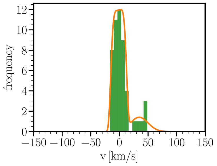
Figure 5: The velocity distribution function (VDF) of one of the bins of our heavily disrupted SMC-analogue simulation (green histogram) and the best Binulator fit to this bin (orange line). Notice that the data are well-fit by the sum of a generalised Gaussian (representing the bound stars of the dwarf; larger bump around $v\sim 0$ km/s) and an additional Gaussian (representing the tidal debris; smaller bump around $\sim 30$ km/s). Note, further, that we do not actually use this best-fit VDF. Rather, we use the the median and 68% confidence intervals of the Binulator fit to generate the velocity dispersion profiles and their uncertainties.

4 Results

4.1 Tests on the simulated SMC-analogues

Before applying our methodology (§3) to the real SMC data, we first test it on simulated mock SMC analogues. We consider two mocks, as described in §2.2: a bound SMC that has undergone very little tidal disruption, and a heavily disrupted SMC that is close to dissolution. This latter is closer to the real situation, but likely even more extreme as the mock SMC has a starting mass lower than the original mass of the SMC (as reconstructed via abundance matching, i.e. in Read & Erkal 2019). As such, it represents a conservative test-case. We first assess how well Binulator can remove unbound tidal debris along the line of sight (§4.1.1); we then apply GravSphere to the mock data to determine how well we can recover the inner Dark Matter density profile and stellar velocity anisotropy (§4.1.2). Other profiles recovered by our models are reported in Appendix A for completeness.

4.1.1 Testing the removal of tidal debris

In Fig. 6, we show the velocity dispersion profiles derived from the heavily disrupted simulation. In the top left panel, we show the results including both bound and unbound stars. In the top right panel, we show results for the same but clipping all stars beyond 2 standard deviations from the dispersion derived for each bin (2$\sigma$ clipped), assuming the original velocity distributions to be Gaussians (see Fig. 1). In the bottom left panel, we show the results obtained by removing the stars with velocity above the escape velocity $V_{esc}$ at their respective position (unbound stars).

$$V_{esc}=\sqrt{-2\Phi(r)}$$ (21)

$$\Phi(r)=-G\int_{r}^{\infty}\frac{M(<r)}{r^{\prime 2}}dr^{\prime}$$ (22)

with $M(r)$ tabulated from the particle data to a very high distance and the integral estimated numerically. Due both to the advanced stage of tidal disruption of the simulation and the discrete mass distribution of the simulation particles, we iterated the selection process until it stopped removing particles. Finally, in the bottom right panel of Fig. 6, we show the profiles derived by the Binulator. The colours of the points in the bottom panels are different because the Binulator transformed the proper motions into the radial and tangential velocities on the plane of the sky and we did the same for the escape velocity cut sample, for ease of comparison (the better kinematically behaved, i.e. bound, sample will always have lower values of the velocity dispersions anyway). As can be seen from the bottom left panel, when removing the stars with velocity higher than the escape velocity, the inner dispersion profiles become consistent with one another: the inner velocity anisotropy of bound stars is isotropic. Sigma clipping of the data in each bin (top right panel) is unable to reproduce this behaviour, with the 2$\sigma$ clipped dispersions remaining significantly tangentially anisotropic, even in the innermost bin. The Binulator (bottom right panel), however, is able to recover the correct behaviour within its statistical uncertainties by removing the unbound stars.

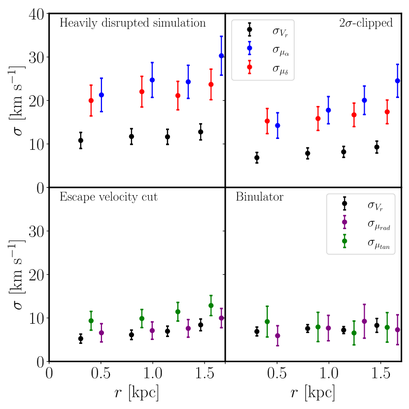
Figure 6: Velocity dispersion profiles for the inner regions of the heavily disrupted simulation. The black points show $\sigma_{vr}$, the blue points $\sigma_{\mu\alpha}$, the red points $\sigma_{\mu\delta}$, the purple points $\mu_{\rm{rad}}$, and the dark green points $\mu_{\rm{tan}}$. Top left panel: velocity dispersions for the full data sample. Top right panel: Velocity dispersions after $2\sigma$-clipping the velocity distributions, which are assumed to be Gaussians (see Fig. 1). Bottom left panel: velocity dispersions after iterated escape velocity cuts. Bottom right panel: velocity dispersions after the decontamination done by the Binulator. Inside each panel the bins are the same but are displaced artificially along the X-axis for clarity.

4.1.2 Testing the mass modelling

In this section, we now apply GravSphere to model the mock data surface brightness and velocity dispersion profiles extracted using Binulator (§3.3). The results for the bound simulation that has not experienced any significant tidal forces are shown in the top row of Fig. 7 while the bottom row is for the heavily disrupted simulation. The left and right columns of the figure show the recovered median (black line), 68% (dark grey), and 95% (light grey) confidence intervals for $\rho(r)$ and $\widetilde{\beta}(r)$, respectively, as compared to the true solutions (blue data points and dashed lines). As can be seen, GravSphere correctly recovers all three within its 95% confidence intervals.

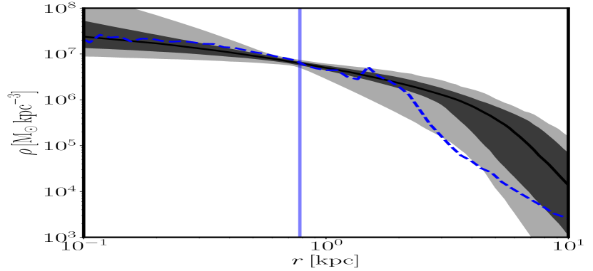
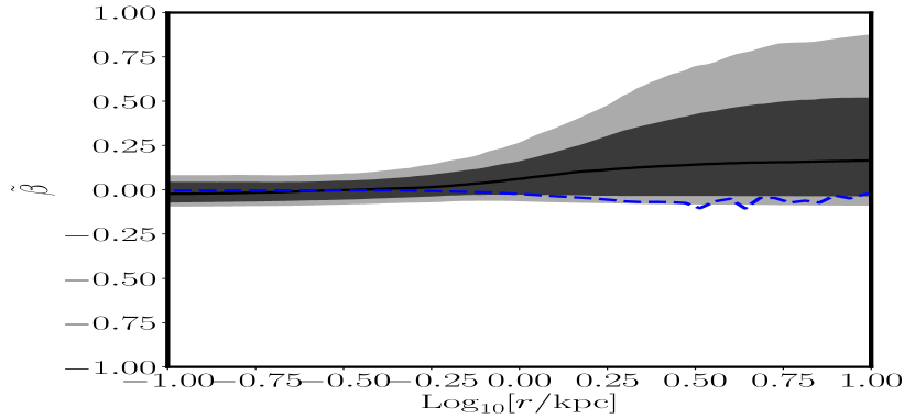
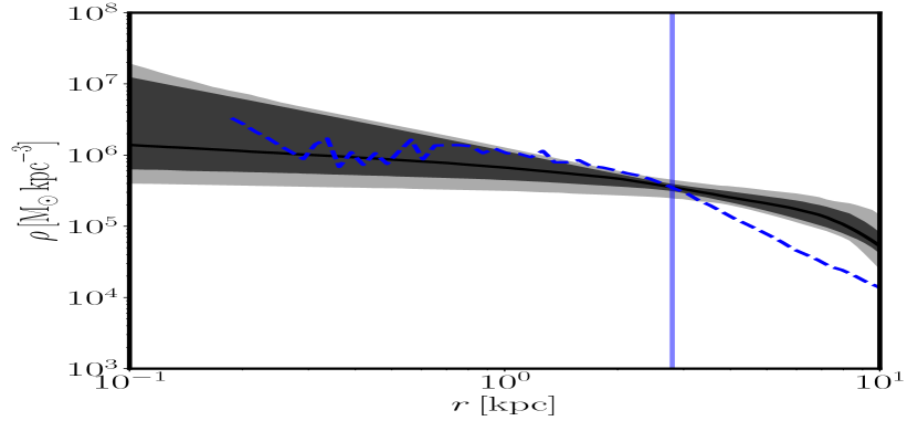
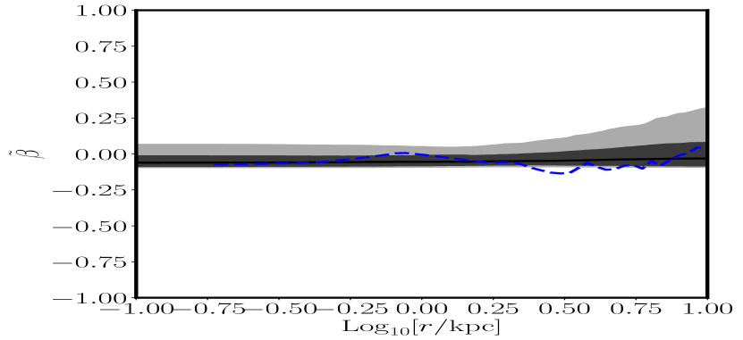
Figure 7: Left panels: recovered mass density profile, $\rho(r)$, of the bound (top) and heavily disrupted (bottom) simulations. The black lines and grey contours mark the median, 68% (dark grey) and 95% (light grey) confidence intervals of the GravSphere fit, respectively. The blue dashed lines show the profiles computed from the simulation data. The blue vertical lines mark the half-stellar mass radius computed by Binulator. Right panels: recovered symmetrised anisotropy profile $\widetilde{\beta}(r)$ for the bound (top) and heavily disrupted (bottom) simulations. The solid black lines, grey contours, vertical blue line and blue dashed lines are as in the left panels.

Fig. 7 shows that GravSphere is able to recover the density and velocity anisotropy profiles within its 95% confidence intervals for both the bound simulation (top panels) and the heavily disrupted simulation (bottom panels) within the half-stellar mass radius (vertical blue line, $R_{1/2}$). Beyond $R_{1/2}$, the recovered density profile is biased high for the heavily disrupted simulation as compared to the true solution (see Fig. 7, bottom left panel), while the velocity anisotropy profile also fluctuates slightly outside of the 95% confidence intervals (bottom right panel). This behaviour is to be expected given that the heavily disrupted simulation becomes unbound beyond $R_{1/2}$, with the percentage of bound stars quickly dropping below $90\%$ outside 1.7 kpc.

4.2 Mass modelling of the real SMC

In this section, we show and discuss the principal results of our modelling of the SMC, namely the successful decontamination with the Binulator, the recovery of the mass density and velocity anisotropy profile and further insights derived from these two variables. Other profiles recovered by our models are reported in Appendix A for completeness.

4.2.1 Removing tidal debris

We first check the impact of the removal of tidal debris by the Binulator. Fig. 8 compares the dispersions of the data processed by the Binulator (right) with the dispersion profiles of the observed data, taken as simple variances of each data bin (left). The decontamination has dampened the tangential anisotropy, with only some mild residual anisotropy remaining at intermediate radii. This is reminiscent of the behaviour of the heavily disrupted mock in Fig. 6.

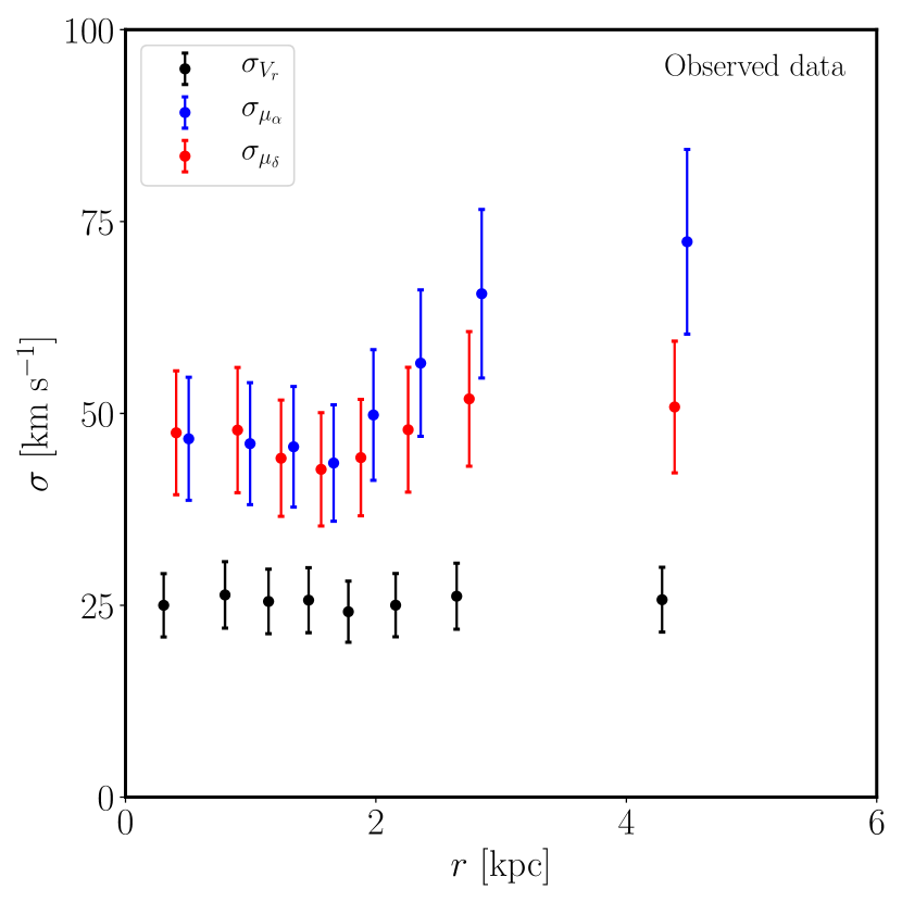
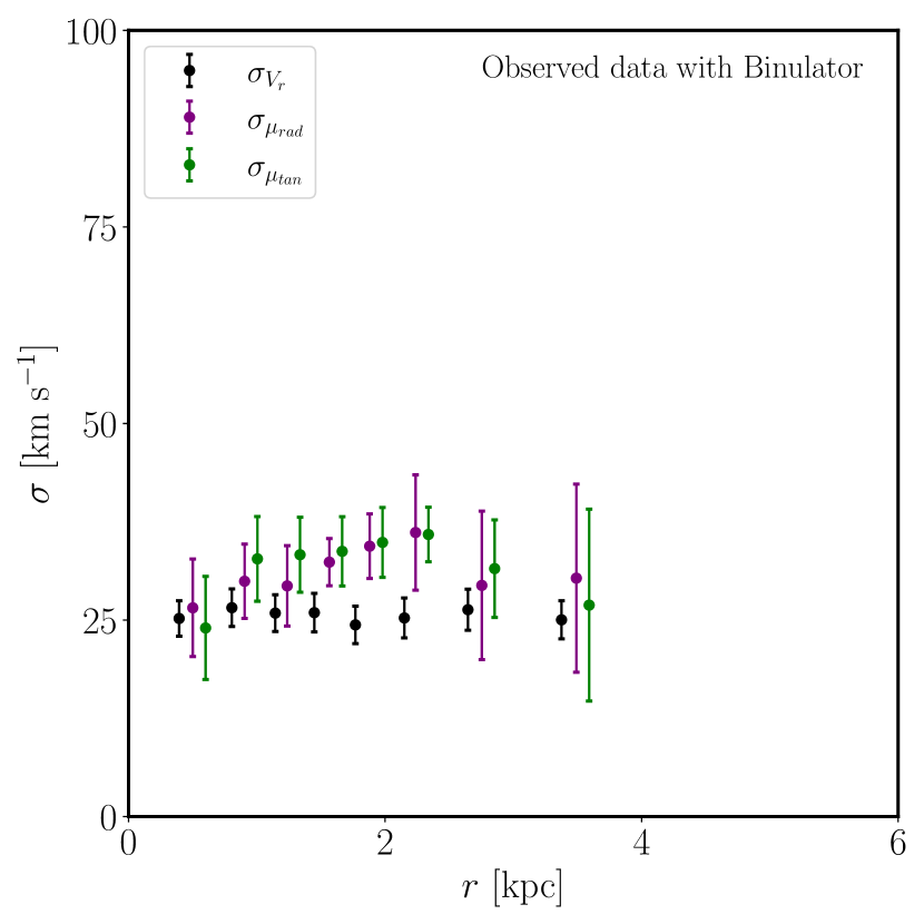
Figure 8: Left panel: dispersion profiles of $V_{r}$ (black points), $\mu_{\alpha}$ (blue points), and $\mu_{\delta}$ (red points) for the observed data. The data are binned at the same positions but displaced along the X-axis for clarity. Right panel: dispersion profiles of $V_{r}$ (black points), $\mu_{\rm{rad}}$ (purple points), and $\mu_{\rm{tan}}$ (dark green points) for the observed data after the Binulator fit of the velocity distributions. The data are binned at the same positions but displaced along the X-axis for clarity.

4.2.2 The GravSphere model of the SMC

In Fig. 9, we show the GravSphere recovery of the Dark Matter density (left) and velocity anisotropy (right) profiles for the real SMC. As reflected in the data (Fig. 8), GravSphere favours some mild tangential anisotropy, though at 95% confidence it is consistent with being isotropic at all radii probed. The density profile is well-constrained over the range $0.5\lesssim R/R_{1/2}\lesssim 2$ and appears more cusp-like than cored (constant density). We discuss this further in §4.2.4.

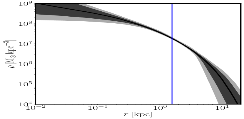
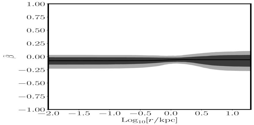
Figure 9: Left panel: $\rho(r)$ profile recovered by GravSphere for the SMC data. The black line is the best fit solution and the dark and light gray regions are, respectively, the 68% and 95% confidence intervals. The faint blue vertical line is the recovered half-light radius. Right panel: $\widetilde{\beta}(r)$ profile recovered by GravSphere for the SMC data. The black line is the best fit solution and the dark and light gray regions are, respectively, the 68% and 95% confidence intervals.

4.2.3 The present and pre-infall mass of the SMC

Regarding the mass of the SMC, the recovered density profile suggests a Dark Matter mass within $3$ kpc of $M_{DM}(\leq 3\,{\rm kpc})=1.48^{+0.08}_{-0.07}\times 10^{9}M_{\odot}$ and a stellar mass within the same radius of $M_{*}(\leq 3\,{\rm kpc})=0.30\pm 0.05\times 10^{9}M_{\odot}$. We compare this with other literature estimates in §5.2.

GravSphere also provides us with constraints on the halo virial mass, $M_{200}=1.71_{-0.50}^{+1.22}\times 10^{10}M_{\odot}$ (see Fig. 10), and concentration parameter, $c_{200}=16.58\pm 7.06$.

Given the extensive tidal disruption experienced by the SMC, it is not entirely clear how we should interpret the recovered $M_{200}$ from present-day dynamical tracers. GravSphere does attempt to model the impact of tidal stripping through the tidal radius and density fall off model parameters, $r_{t}$ and $\delta$ (see §3 and Equation  8). Unfortunately, we could not obtain constraints on $r_{t}$ and $\delta$ that are bound only by our priors. Furthermore, GravSphere is not able to account for historic mass loss from inside $r_{t}$, neither from tidal stripping nor tidal shocks (e.g. Read et al., 2006). As such, any estimate of $M_{200}$ will be a lower bound on the SMC’s pre-infall halo mass.

Despite the above caveats, GravSphere yields an estimate of the SMC’s pre-infall $M_{200}$ that overlaps, within our 95% confidence intervals, with that obtained from abundance matching (e.g. Read & Erkal, 2019): $M_{200,{\rm abund}}=7.73\pm 1.69\times 10^{10}M_{\odot}$ (see the solid and dashed red lines in Fig. 10 that mark the median and $\pm 68\%$ confidence intervals of $M_{200,{\rm abund}}$).

Considering the, likely more robust, pre-infall $M_{200,{\rm abund}}$ estimation, our recovered $c_{200}$ parameter is consistent (within the 68% uncertainty) with the value expected in $\Lambda$CDM ($\sim$11 from Dutton & Macciò, 2014) for a galaxy of the halo mass of the pre-infall SMC.

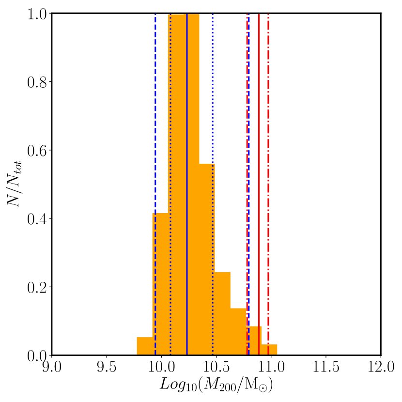
Figure 10: Distribution of the $M_{200}$ values recovered by GravSphere (orange histogram). The mean value of the distribution is marked by the solid blue line, the dotted blue lines denote the 68% confidence interval while the dashed blue lines indicate the 95% confidence interval. The value reported by Read & Erkal (2019) is marked by a solid red line with its 68% confidence interval denoted by the dot-dashed red lines.

4.2.4 The inner Dark Matter density of the SMC: testing Dark Matter heating models

Armed with our recovered Dark Matter density profile and $M_{200}$ for the SMC, we now turn to its position in the $\rho_{\rm DM}$-$M_{200}$ plane. As first proposed in Read et al. (2019) (and see also §1), this provides a key test of “Dark Matter heating” models. For $M_{200}$, we will use the abundance matching pre-infall halo mass for the SMC: $M_{200,{\rm abund}}=7.73\pm 1.69\times 10^{10}M_{\odot}$ (Read & Erkal, 2019). As discussed above, this is likely to be a more reliable estimate than that based on the SMC’s current dynamical state.

Fig. 11 compares the theoretical expectations for perfectly preserved Dark Matter cusps in a $\Lambda$CDM cosmology (gray bands) and complete cusp-core transformations due to Dark Matter heating (light blue bands) with the data from (Read et al., 2019) (black, blue and purple circles) and the SMC (red square). The left panel shows estimates of the Dark Matter density at 150 pc from the centres of the galaxies; the right panel at 500 pc. The black symbols are galaxies that stopped forming stars more than 6 Gyrs ago, the purple symbol is a galaxy that stopped forming stars $3-6$ Gyrs ago and the blue symbols are galaxies that stopped forming stars in the last 3 Gyrs. All galaxies have been selected to be tidally isolated today (see Read et al. 2019).

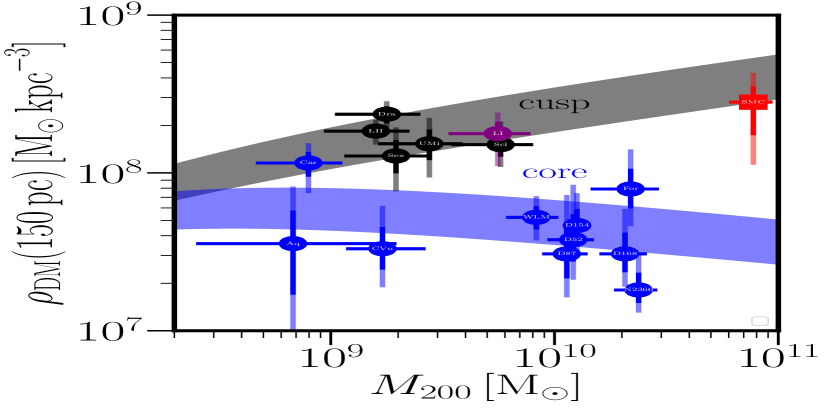
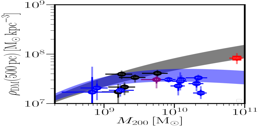
Figure 11: Left panel: Inner Dark Matter density (at 150pc) as a function of halo mass for a sample of dwarf galaxies. The gray band marks the theoretical expectation for perfectly preserved cusps (no Dark Matter heating) while the light blue band denotes the expectation for complete core transformation (maximal Dark Matter heating). The black symbols are dwarf galaxies that stopped forming stars more than 6 Gyrs ago, the purple symbol is a galaxy that stopped forming stars between 6 and 3 Gyrs ago, the blue symbols are galaxies that stopped forming stars in the last 3 Gyrs and the red square is the SMC. The error bars for the symbols are fully coloured for $1\sigma$ value and faintly coloured up to the $2\sigma$ value. Right panel: same as the left panel but for the density estimated at 500pc (instead of 150pc).

Firstly, notice that at low $M_{200}$ the blue and black bands overlap. This is because the Dark Matter core size scales with $\sim R_{1/2}$ which in turn correlates with $M_{200}$. As $M_{200}$ is reduced, the expected core size shrinks and at a fixed length scale, the cusped and cored models begin to overlap. This happens at even higher mass for the $\rho_{\rm DM}(500\,{\rm pc})$ plot (right panel). Secondly, notice that the black and purple data points, corresponding to galaxies whose star formation shut down long ago, are consistent with dense Dark Matter cusps. By contrast, those dwarfs with recent star formation (blue data points) have had the most Dark Matter heating and are consistent with fully formed Dark Matter cores. The SMC, however, (red data point) has a much higher pre-infall $M_{200}$ than any of the data points taken from Read et al. (2019); it has a central density consistent with a Dark Matter cusp, not a core. This can be seen both at 150 pc where the errors are quite substantial (left panel), and even more clearly at 500 pc where the density profile is better-constrained (right panel).

We now consider whether the above behaviour – galaxies moving from being cusped to cored and then back to cusped again – is consistent with Dark Matter heating models. To test this, we switch from the $\rho_{\rm DM}$-$M_{200}$ plane to the $\rho_{\rm DM}$-$M_{*}/M_{200}$ plane. As discussed in §1, $M_{*}/M_{200}$ – to leading order – indicates how much energy is available to drive Dark Matter heating (e.g. Peñarrubia et al., 2012). We expect Dark Matter heating to increase with increasing $M_{*}/M_{200}$ until the self-gravity of the stars begins to dominate over the Dark Matter at which point Dark Matter heating becomes inefficient again (e.g. Di Cintio et al., 2014a). In Fig. 12, we combine our data for the SMC with literature data from Read et al. 2019, Bouché et al. 2022 (courtesy of N. F. Bouché) and Cooke et al. 2022 (courtesy of R. C. Levy) to explicitly test this. We can see from Fig. 12 the relationship between central Dark Matter density at 150 pc and the stellar-to-halo mass ratio, $M_{*}/M_{200}$, for the data (squares and stars) as compared to several different models (coloured lines). The colours denote tracks of constant $M_{200}$, as marked by the colourbars. The data points are coloured similarly by their median $M_{200}$, as estimated from abundance matching. The top left panel of Fig. 12 shows a classical NFW model (Navarro et al., 1996b) without Dark Matter heating. This model fits the more dense ‘cusp’-like dwarfs, but fails to reproduce the lower density ‘core’-like dwarfs in the range: $5\times 10^{-4}\lesssim M_{*}/M_{200}\lesssim 10^{-2}$. The top right panel of Fig. 12 shows the Di Cintio et al. (2014b) model which correctly reproduces the qualitative behaviour seen in the data, with cusp-like densities below $M_{*}/M_{200}\lesssim 5\times 10^{-4}$, core-like densities in the range $5\times 10^{-4}\lesssim M_{*}/M_{200}\lesssim 5\times 10^{-3}$ and cusp-like densities again for $M_{*}/M_{200}\gtrsim 5\times 10^{-3}$. However, there are quantitative differences, with the model favouring a slower and smoother transition between the cusped and cored regimes (and back again) as compared to the data (for example, cusp-like densities at $M_{*}/M_{200}\sim 5\times 10^{-4}$ are not expected by the model). We must note that the model has been computed assuming the median concentration parameter, $c_{200}$, in a $\Lambda$CDM cosmology (Dutton & Macciò, 2014). This may not be appropriate for the dwarf spheroidal satellites of the Milky Way that likely fell in long ago (Read & Erkal, 2019) and may, therefore, be biased to higher concentration parameters (e.g. Springel et al., 2008). If we assume instead concentration parameters biased $2-\sigma$ above the median, we find that the model does pass comfortably through the data points for the dwarf spheroidals at low $M_{*}/M_{200}<10^{-3}$ (see Appendix C). A similar effect may explain the same discrepancy between the model and the high density we recover for the SMC. Whether this is the correct interpretation of the behaviour of these data, or whether the Dark Matter heating model of Di Cintio et al. (2014a) is not quite correct, remains to be seen.

The bottom left panel of Fig. 12 shows the Lazar et al. (2020) model which correctly reproduces the behaviour seen in the data up until $M_{*}/M_{200}\sim 10^{-2}$, but fails to account for the more dense halos at higher mass ratios. The errors for most of these higher mass ratio data points remain large, but the data point we derive here for the SMC certainly seems to be in significant tension with the Lazar et al. (2020) prediction. This highlights two important points: (i) not all Dark Matter heating models in the literature make the same predictions; and (ii) the latest data are now able to quantitatively test these models.

Finally, in the bottom right panel of Fig. 12 we show a handy analytic function, built on the coreNFW profile (equation 10), that captures the main features of the data. This introduces an $M_{*}/M_{200}$ dependence on the $n$ parameter (that determines how cusped or cored the profile is):

$$n=\kappa_{3}\exp\left(\frac{-(\rm{Log}_{10}(M_{*}/M_{200})-\kappa_{1})^{2}}{\kappa_{2}}\right)$$ (23)

where $\kappa_{1}=-2.75$, $\kappa_{2}=0.2$ and $\kappa_{3}=1.25$. Readers may find this useful as a compact analytic description of the behaviour of the data and/or to test their own favoured models.

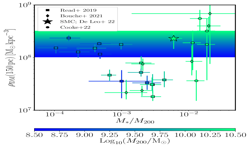
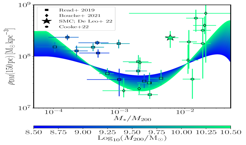
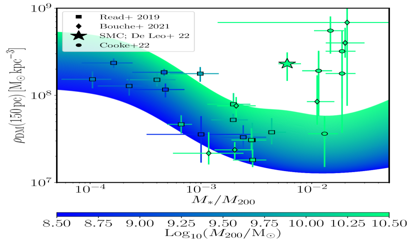
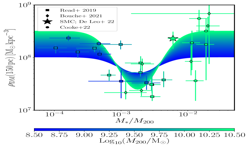
Figure 12: Central Dark Matter density $\rho_{DM}$ at 150 pc from the galactic centre against stellar-to-halo mass ratio $M_{*}/M_{200}$ for the data presented in Read & Erkal (2019), Bouché et al. (2022), Cooke et al. (2022) and the SMC (the coloured symbols) compared to different Dark Matter models (coloured bands). In all panels, the colour of the points and of specific positions along the bands marks the pre-infall halo mass, $M_{200}$ (see the colourbar). Top left panel: the band is the prediction of the Navarro et al. (1996b) model. Top right panel: the band is the prediction of the Di Cintio et al. (2014b) model. Bottom left panel: the band is the prediction of the Lazar et al. (2020) model. Bottom right panel: the band is a modified coreNFW model tuned to the data.

4.2.5 The astrophysical $J$-factor and $D$-factor of the SMC

Given their dense environments, dwarf galaxies can be suitable candidates for searches of Dark Matter annihilation and/or decay events (Kuhlen, 2010) so we will conclude this section with a look at the SMC in this context. The density estimation of GravSphere can be used to derive the $J$-factor: the integral of the square of the Dark Matter density along the line-of-sight and over a solid angle $\delta\Omega$ (Alvarez et al., 2020). This parameter quantifies the dependence of Dark Matter annihilation searches on the density of the astrophysical target being searched. We recovered the distribution of $J$-factors for the SMC, shown in Fig. 13. This has a mean of $19.22\pm 0.14$  GeV² cm^-5, shown as the solid red line in the figure. We also recovered the distribution of the $D$-factor: the integral of the Dark Matter density along the line-of-sight and over a solid angle $\delta\Omega$ (Alvarez et al., 2020). This is the relevant quantity for testing decaying Dark Matter models. We find a mean value of $18.80\pm 0.03$  GeV² cm^-5. Both of these are interestingly competitive with the densest dwarfs known to date around the Milky Way (e.g. Alvarez et al., 2020), suggesting that the SMC is a prime target for such annihilation and decay searches.

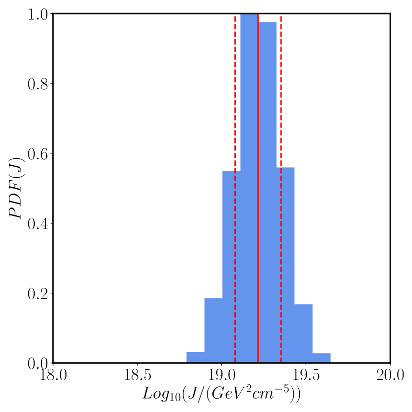
Figure 13: The PDF for the $J$-factor recovered by GravSphere (blue histogram). The mean value of the distribution is marked as a solid red line with dashed red lines marking the 68% confidence interval.

5 Discussion

5.1 The impact of priors

Before delving deeper in the information that can be extracted from the mass model of the SMC, it is worth discussing briefly the choices of priors operated throughout the modeling process and how they affect the results. The flat priors assumed for the mass profile (rows 1 to 6 in Tab. 1) were purposefully weak to allow for the recovery of any kind of final model (be it cuspy or cored). The $M_{200}$ and $c_{200}$ bounds were informed by previous studies of the SMC (respectively Read & Erkal 2019 and Besla et al. 2012) while the others were left wide to allow for any possible solution. The priors assumed for the velocity PDFs recovered by the Binulator (rows 13 to 15 of Tab. 1) were informed by our previous study of the SMC bulk motion (De Leo et al., 2020), based on the same observational data. As for the priors on the mass profile, we favoured weaker priors for the anisotropy parameters (rows 9 to 12 of Tab. 1). We found that tighter priors (i.e. $-0.1\leq\beta_{0}\leq 0.1$) produced a slightly more cored density profile at the expense of strongly enforcing a zero value of the central anisotropy profile (see Fig. 16 in Appendix B).

5.2 The present-day mass of the SMC

It is difficult to make a proper comparison of our recovered present-day mass of the SMC with values in the literature as most estimations were derived from mass models that assumed gas and stars were bound by the SMC potential to large radii. We obtain $M_{DM}(\leq 3\,{\rm kpc})=1.48^{+0.08}_{-0.07}\times 10^{9}M_{\odot}$ and $M_{*}(\leq 3\,{\rm kpc})=0.30\pm 0.05\times 10^{9}M_{\odot}$ (§4.2.3). Summing to this the total gas mass measured within the same radius ($5.6\times 10^{8}M_{\odot}$; Stanimirovic et al. 1999; Stanimirović et al. 2004; Brüns et al. 2005), we obtain a total present-day mass of the SMC equal to $M_{{\rm tot}}(\leq 3\,{\rm kpc})=2.34\pm 0.46\times 10^{9}M_{\odot}$. While this value is consistent with the estimate for total SMC mass of $2.4\times 10^{9}M_{\odot}$ in Stanimirović et al. (2004), the underlying assumptions of our methods are quite different (the model in Stanimirović et al. 2004 was a two-component model without Dark Matter) so it is challenging to meaningfully compare the two values. Our total mass is also consistent with the lower bound of the estimation from Harris & Zaritsky (2006), who derived a total mass between $2.7\times 10^{9}M_{\odot}$ and $5.1\times 10^{9}M_{\odot}$ through a simple virial analysis based on stellar kinematics. The smaller value that we recover is due to the fact our model excludes the stars in the tidal debris from the computation of the bound SMC mass.

5.3 Comparison with Dark Matter annihilation literature

Our recovered value for the $J$-factor ($19.22\pm 0.14$  GeV² cm^-5) is in good agreement with the estimate of Caputo et al. (2016) and – interestingly – on par with the isolated dwarf galaxy Draco ($18.69\pm 0.05$  GeV² cm^-5 estimated in Alvarez et al., 2020). The estimated $D$-factor ($18.80\pm 0.03$  GeV² cm^-5) likewise is consistent with estimations for isolated dwarf galaxies (Draco, Tucana II estimated in Evans et al., 2016). This suggests that the SMC is a competitive target for the observation of gamma-rays and/or X-rays originating from Dark Matter annihilation and/or decay events.

6 Conclusions

Using mock data we showed that, despite being subjected to heavy tidal disruption, the SMC can still be mass modelled with methods that require dynamical equilibrium. For this, we assumed that the galaxy is composed of a central bound remnant surrounded by tidal debris (as supported by the latest observational data, e.g. Graczyk et al. 2020). Given that building an unbiased mass model requires a careful removal of tidal debris along the line-of-sight, we introduced the Binulator. This new method to achieve the decontamination successfully worked on the mock data.

We then proceeded to apply a Jeans mass modelling method (Binulator+GravSphere) to ${\sim}6000$ RGB stars with spectroscopic and proper motion data from Gaia Early Data Release 3 (EDR3) to build a new mass model of the Small Magellanic Cloud (SMC). The data decontamination employed by the Binulator and the use of the full dynamical information (the line-of-sight velocity distribution and proper motions) by GravSphere were instrumental in recovering a robust model which we could use to further explore the characteristics of the Dark Matter halo of the SMC. After the removal of the tidally unbound interlopers, we recovered both the mass density and the stellar velocity anisotropy profile (which shows the remaining stars to be isotropic at all radii within the uncertainties).

We provided a new estimate for the total present-day mass of the SMC, $M_{{\rm tot}}(\leq 3\,{\rm kpc})=2.34\pm 0.46\times 10^{9}M_{\odot}$, based on stellar kinematics, that takes into account the extensive tidal disruption undergone by the galaxy.

Our model found that the SMC has a high central density, $\rho_{\rm DM}(150\,{\rm pc})=2.81_{-1.07}^{+0.72}\times 10^{8}M_{\odot}\rm kpc^{-3}$, which is consistent with a Dark Matter cusp within the $\Lambda$CDM paradigm (this is true down to at least 400 pc from the galaxy’s centre). The inferred Dark Matter density profile provides an observational reference point for the halo mass scale at which Dark Matter heating becomes inefficient and is no longer able to drive a cusp-core transformation.

We used the SMC, together with previously available data, to test Dark Matter heating models in the literature, finding good qualitative agreement with the Di Cintio et al. (2014a) model but poorer agreement with the Lazar et al. (2020) model at $M_{*}/M_{200}>10^{-2}$. We also introduced a new analytic density profile that gives a good fit to the central Dark Matter density of dwarf galaxies and its dependence on $M_{*}/M_{200}$.

Finally, from the recovered cuspy Dark Matter density profile, we derived an astrophysical $J$-factor of $19.22\pm 0.14$  GeV² cm^-5 ($D$-factor of $18.80\pm 0.03$  GeV² cm^-5), suggesting that the SMC is a very promising target for Dark Matter annihilation and decay searches.

Data Availability Statement

The data underlying this article will be shared on reasonable request to the corresponding author.

Appendix A GravSphere recovered profiles

In this appendix, we show the surface brightness profile and the three velocity profiles (line-of-sight, radial and tangential) recovered by GravSphere for the case of the heavily disrupted simulation (Fig. 14) and for the real SMC (Fig. 15).

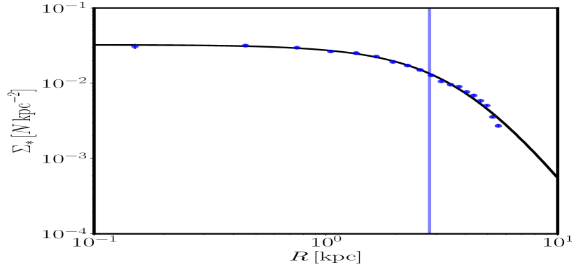
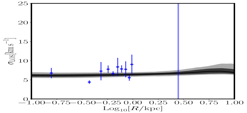
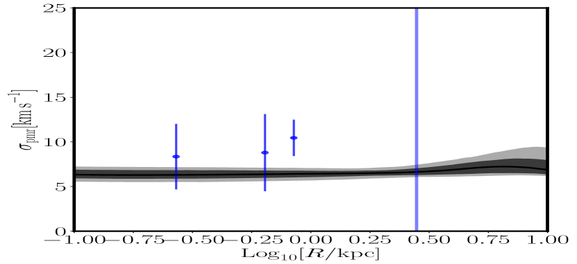
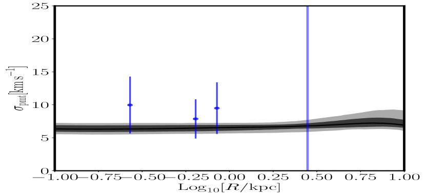
Figure 14: GravSphere recovered profiles for the heavily disrupted simulation. Top left panel: surface brightness $\Sigma_{*}(r)$. The black line is the GravSphere fit, the blue points are the simulation data and the faint blue line marks the half-light radius computed by GravSphere. Top right panel: velocity dispersion profile along the line of sight $\sigma_{LOS}$, the black line is GravSphere best fit solution, the dark and light grey contour are respectively the 68% and the 95% confidence intervals, the blue points with error bars are the binned data and the faint blue line marks the half-light radius computed by GravSphere. Bottom left panel: radial velocity dispersion profile $\sigma_{rad}$, lines and symbols are the same as for $\sigma_{LOS}$. Bottom right panel: tangential velocity dispersion profile $\sigma_{tan}$, lines and symbols are the same as for $\sigma_{LOS}$.

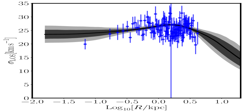
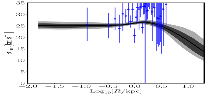
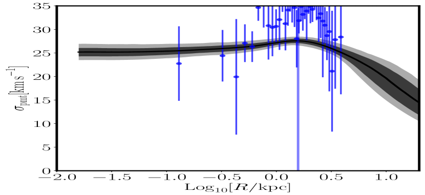
Figure 15: GravSphere recovered profiles for the real SMC. Top left panel: surface brightness $\Sigma_{*}(r)$. The black line is the GravSphere fit, the blue points with errorbars are the observed SMASH data and the faint blue line marks the half-light radius computed by GravSphere. Top right panel: velocity dispersion profile along the line of sight $\sigma_{LOS}$, the black line is GravSphere best fit solution, the dark and light grey contour are respectively the 68% and the 95% confidence intervals, the blue points with error bars are the binned data and the faint blue line marks the half-light radius computed by GravSphere. Bottom left panel: velocity dispersion profile along the radial direction $\sigma_{rad}$, lines and symbols are the same as for $\sigma_{LOS}$. Bottom right panel: velocity dispersion profile along the tangential direction $\sigma_{tan}$, lines and symbols are the same as for $\sigma_{LOS}$.

Appendix B Different priors

As discussed in the main text in Sec. 5.1, we tested the effect of different priors on our parameter recovery. Most of the tests (changing the bounds of the priors on $n$ or restricting to smaller maximum $r_{c}$ or $r_{t}$) had negligible impact on our models. The most impactful prior choice was on $\beta_{0}$, specifically on enforcing a tighter prior with $-0.1\leq\beta_{0}\leq 0.1$. This change had a minor impact on the recovered mass density profile, $\rho(r)$, as can be seen in Fig. 16. Notice that the density profile (left) now permits a small inner core within the 95% confidence intervals. However, beyond $r>400$ pc, the results are in good agreement with our default broader priors (see Figure 9).

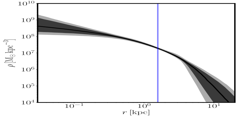
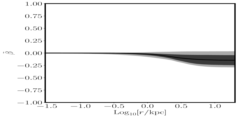
Figure 16: Same as Fig. 9: the mass density profile, $\rho(r)$, (left panel) and the symmetrised anisotropy profile, $\widetilde{\beta}(r)$, (right panel) recovered by GravSphere for the SMC data but for a model with prior $-0.1\leq\beta_{0}\leq 0.1$. Notice that the density profile (left) now permits a small inner core within the 95% confidence intervals. However, beyond $r>400$ pc, the results are in good agreement with our default broader priors (see Figure 9).

Appendix C Concentration parameter bias

In this appendix we show how a 2-$sigma$ bias in the estimation of the concentration parameter $c_{200}$ can reconcile the Di Cintio et al. (2014b) model with the observational data in the $M_{*}/M_{200}<10^{-3}$ range (Fig. 17).

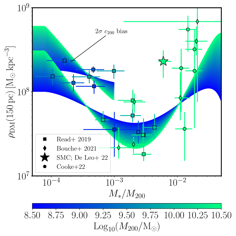
Figure 17: Same as the top right corner of Fig. 12 but with the addition of an hypothetical $c_{200}$ bias.

References

- Allende Prieto et al. (2018) Allende Prieto C., Koesterke L., Hubeny I., Bautista M. A., Barklem P. S., Nahar S. N., 2018, A&A, 618, A25
- Alvarez et al. (2020) Alvarez A., Calore F., Genina A., Read J., Serpico P. D., Zaldivar B., 2020, J. Cosmology Astropart. Phys., 2020, 004
- Astropy Collaboration et al. (2013) Astropy Collaboration et al., 2013, A&A, 558, A33
- Astropy Collaboration et al. (2018) Astropy Collaboration et al., 2018, AJ, 156, 123
- Avila-Reese et al. (2001) Avila-Reese V., Colín P., Valenzuela O., D’Onghia E., Firmani C., 2001, ApJ, 559, 516
- Baes & van Hese (2007) Baes M., van Hese E., 2007, A&A, 471, 419
- Besla et al. (2012) Besla G., Kallivayalil N., Hernquist L., van der Marel R. P., Cox T. J., Kereš D., 2012, MNRAS, 421, 2109
- Binney (1980) Binney J., 1980, MNRAS, 190, 873
- Binney & Mamon (1982) Binney J., Mamon G. A., 1982, MNRAS, 200, 361
- Binney & Tremaine (2008) Binney J., Tremaine S., 2008, Galactic dynamics. Princeton, NJ: Princeton University Press, 2008
- Bode et al. (2001) Bode P., Ostriker J. P., Turok N., 2001, ApJ, 556, 93
- Bouché et al. (2022) Bouché N. F., et al., 2022, A&A, 658, A76
- Bovy (2015) Bovy J., 2015, ApJS, 216, 29
- Brüns et al. (2005) Brüns C., et al., 2005, A&A, 432, 45
- Caputo et al. (2016) Caputo R., Buckley M. R., Martin P., Charles E., Brooks A. M., Drlica-Wagner A., Gaskins J., Wood M., 2016, Phys. Rev. D, 93, 062004
- Carrera et al. (2017) Carrera R., Conn B. C., Noël N. E. D., Read J. I., López Sánchez Á. R., 2017, MNRAS, 471, 4571
- Collins & Read (2022) Collins M. L. M., Read J. I., 2022, Nature Astronomy, 6, 647
- Collins et al. (2021) Collins M. L. M., et al., 2021, MNRAS, 505, 5686
- Cooke et al. (2022) Cooke L. H., et al., 2022, MNRAS, 512, 1012
- De Leo et al. (2020) De Leo M., Carrera R., Noël N. E. D., Read J. I., Erkal D., Gallart C., 2020, MNRAS, 495, 98
- Di Cintio et al. (2014a) Di Cintio A., Brook C. B., Macciò A. V., Stinson G. S., Knebe A., Dutton A. A., Wadsley J., 2014a, MNRAS, 437, 415
- Di Cintio et al. (2014b) Di Cintio A., Brook C. B., Dutton A. A., Macciò A. V., Stinson G. S., Knebe A., 2014b, MNRAS, 441, 2986
- Dobbie et al. (2014) Dobbie P. D., Cole A. A., Subramaniam A., Keller S., 2014, MNRAS, 442, 1663
- Dubinski & Carlberg (1991) Dubinski J., Carlberg R. G., 1991, ApJ, 378, 496
- Dutton & Macciò (2014) Dutton A. A., Macciò A. V., 2014, MNRAS, 441, 3359
- El-Badry et al. (2016) El-Badry K., Wetzel A., Geha M., Hopkins P. F., Kereš D., Chan T. K., Faucher-Giguère C.-A., 2016, ApJ, 820, 131
- El-Zant et al. (2001) El-Zant A., Shlosman I., Hoffman Y., 2001, ApJ, 560, 636
- Emami et al. (2019) Emami N., Siana B., Weisz D. R., Johnson B. D., Ma X., El-Badry K., 2019, ApJ, 881, 71
- Erkal et al. (2019) Erkal D., et al., 2019, MNRAS, 487, 2685
- Evans & Howarth (2008) Evans C. J., Howarth I. D., 2008, MNRAS, 386, 826
- Evans et al. (2016) Evans N. W., Sanders J. L., Geringer-Sameth A., 2016, Phys. Rev. D, 93, 103512
- Flores & Primack (1994) Flores R. A., Primack J. R., 1994, ApJ, 427, L1
- Foreman-Mackey et al. (2013) Foreman-Mackey D., Hogg D. W., Lang D., Goodman J., 2013, PASP, 125, 306
- Gaia Collaboration et al. (2018) Gaia Collaboration et al., 2018, A&A, 616, A1
- Gaia Collaboration et al. (2021) Gaia Collaboration et al., 2021, A&A, 649, A1
- Genina et al. (2018) Genina A., et al., 2018, MNRAS, 474, 1398
- Genina et al. (2020) Genina A., et al., 2020, MNRAS, 498, 144
- Gnedin & Zhao (2002) Gnedin O. Y., Zhao H., 2002, MNRAS, 333, 299
- Górski et al. (2005) Górski K. M., Hivon E., Banday A. J., Wandelt B. D., Hansen F. K., Reinecke M., Bartelmann M., 2005, ApJ, 622, 759
- Graczyk et al. (2020) Graczyk D., et al., 2020, ApJ, 904, 13
- Gregory et al. (2020) Gregory A. L., et al., 2020, MNRAS, 496, 1092
- Harris & Zaritsky (2006) Harris J., Zaritsky D., 2006, AJ, 131, 2514
- Harris et al. (2020) Harris C. R., et al., 2020, Nature, 585, 357
- Hatzidimitriou et al. (1993) Hatzidimitriou D., Cannon R. D., Hawkins M. R. S., 1993, MNRAS, 261, 873
- Hogan & Dalcanton (2000) Hogan C. J., Dalcanton J. J., 2000, Phys. Rev. D, 62, 063511
- Hunter (2007) Hunter J. D., 2007, Computing in Science and Engineering, 9, 90
- Jacyszyn-Dobrzeniecka et al. (2016) Jacyszyn-Dobrzeniecka A. M., et al., 2016, Acta Astron., 66, 149
- Jacyszyn-Dobrzeniecka et al. (2017) Jacyszyn-Dobrzeniecka A. M., et al., 2017, Acta Astron., 67, 1
- Jeans (1922) Jeans J. H., 1922, MNRAS, 82, 122
- Kauffmann (2014) Kauffmann G., 2014, MNRAS, 441, 2717
- Klimentowski et al. (2007) Klimentowski J., Łokas E. L., Kazantzidis S., Prada F., Mayer L., Mamon G. A., 2007, MNRAS, 378, 353
- Kuhlen (2010) Kuhlen M., 2010, Advances in Astronomy, 2010, 162083
- Lazar et al. (2020) Lazar A., et al., 2020, MNRAS, 497, 2393
- Leaman et al. (2012) Leaman R., et al., 2012, ApJ, 750, 33
- Lindegren et al. (2018) Lindegren L., et al., 2018, A&A, 616, A2
- Lindegren et al. (2021) Lindegren L., et al., 2021, A&A, 649, A2
- Mamon & Łokas (2005) Mamon G. A., Łokas E. L., 2005, MNRAS, 363, 705
- Martizzi et al. (2013) Martizzi D., Teyssier R., Moore B., 2013, MNRAS, 432, 1947
- Mashchenko et al. (2008) Mashchenko S., Wadsley J., Couchman H. M. P., 2008, Science, 319, 174
- Massana et al. (2020) Massana P., et al., 2020, MNRAS, 498, 1034
- McConnachie (2012) McConnachie A. W., 2012, AJ, 144, 4
- Merrifield & Kent (1990) Merrifield M. R., Kent S. M., 1990, AJ, 99, 1548
- Moore (1994) Moore B., 1994, Nature, 370, 629
- Muraveva et al. (2018) Muraveva T., et al., 2018, MNRAS, 473, 3131
- Navarro et al. (1996a) Navarro J. F., Eke V. R., Frenk C. S., 1996a, MNRAS, 283, L72
- Navarro et al. (1996b) Navarro J. F., Frenk C. S., White S. D. M., 1996b, ApJ, 462, 563
- Navarro et al. (1997) Navarro J. F., Frenk C. S., White S. D. M., 1997, ApJ, 490, 493
- Nidever et al. (2021) Nidever D. L., et al., 2021, AJ, 161, 74
- Niederhofer et al. (2021) Niederhofer F., et al., 2021, MNRAS, 502, 2859
- Noël et al. (2013) Noël N. E. D., Conn B. C., Carrera R., Read J. I., Rix H. W., Dolphin A., 2013, ApJ, 768, 109
- Noël et al. (2015) Noël N. E. D., Conn B. C., Read J. I., Carrera R., Dolphin A., Rix H. W., 2015, MNRAS, 452, 4222
- Oñorbe et al. (2015) Oñorbe J., Boylan-Kolchin M., Bullock J. S., Hopkins P. F., Kereš D., Faucher-Giguère C.-A., Quataert E., Murray N., 2015, MNRAS, 454, 2092
- Olsen et al. (2011) Olsen K. A. G., Zaritsky D., Blum R. D., Boyer M. L., Gordon K. D., 2011, ApJ, 737, 29
- Oman et al. (2019) Oman K. A., Marasco A., Navarro J. F., Frenk C. S., Schaye J., Benítez-Llambay A., 2019, MNRAS, 482, 821
- Orkney et al. (2021) Orkney M. D. A., et al., 2021, MNRAS, 504, 3509
- Peñarrubia et al. (2012) Peñarrubia J., Pontzen A., Walker M. G., Koposov S. E., 2012, ApJ, 759, L42
- Plummer (1911) Plummer H. C., 1911, MNRAS, 71, 460
- Pontzen & Governato (2012) Pontzen A., Governato F., 2012, MNRAS, 421, 3464
- Pontzen & Governato (2014) Pontzen A., Governato F., 2014, Nature, 506, 171
- Read & Erkal (2019) Read J. I., Erkal D., 2019, MNRAS, 487, 5799
- Read & Gilmore (2005) Read J. I., Gilmore G., 2005, MNRAS, 356, 107
- Read & Steger (2017) Read J. I., Steger P., 2017, MNRAS, 471, 4541
- Read et al. (2006) Read J. I., Wilkinson M. I., Evans N. W., Gilmore G., Kleyna J. T., 2006, MNRAS, 367, 387
- Read et al. (2016a) Read J. I., Agertz O., Collins M. L. M., 2016a, MNRAS, 459, 2573
- Read et al. (2016b) Read J. I., Iorio G., Agertz O., Fraternali F., 2016b, MNRAS, 462, 3628
- Read et al. (2017) Read J. I., Iorio G., Agertz O., Fraternali F., 2017, MNRAS, 467, 2019
- Read et al. (2018) Read J. I., Walker M. G., Steger P., 2018, MNRAS, 481, 860
- Read et al. (2019) Read J. I., Walker M. G., Steger P., 2019, MNRAS, 484, 1401
- Read et al. (2021) Read J. I., et al., 2021, MNRAS, 501, 978
- Richardson & Fairbairn (2014) Richardson T., Fairbairn M., 2014, MNRAS, 441, 1584
- Ripepi et al. (2014) Ripepi V., et al., 2014, MNRAS, 442, 1897
- Ripepi et al. (2017) Ripepi V., et al., 2017, MNRAS, 472, 808
- Rojas-Niño et al. (2016) Rojas-Niño A., Read J. I., Aguilar L., Delorme M., 2016, MNRAS, 459, 3349
- Sanders & Evans (2020) Sanders J. L., Evans N. W., 2020, MNRAS, 499, 5806
- Schive et al. (2014) Schive H.-Y., Chiueh T., Broadhurst T., 2014, Nature Physics, 10, 496
- Scowcroft et al. (2016) Scowcroft V., Freedman W. L., Madore B. F., Monson A., Persson S. E., Rich J., Seibert M., Rigby J. R., 2016, ApJ, 816, 49
- Sharp & Birchall (2010) Sharp R., Birchall M. N., 2010, Publ. Astron. Soc. Australia, 27, 91
- Smith et al. (2016) Smith R., Choi H., Lee J., Rhee J., Sanchez-Janssen R., Yi S. K., 2016, ApJ, 833, 109
- Sparre et al. (2017) Sparre M., Hayward C. C., Feldmann R., Faucher-Giguère C.-A., Muratov A. L., Kereš D., Hopkins P. F., 2017, MNRAS, 466, 88
- Spergel & Steinhardt (2000) Spergel D. N., Steinhardt P. J., 2000, Phys. Rev. Lett., 84, 3760
- Springel (2005) Springel V., 2005, MNRAS, 364, 1105
- Springel et al. (2008) Springel V., et al., 2008, MNRAS, 391, 1685
- Stanimirovic et al. (1999) Stanimirovic S., Staveley-Smith L., Dickey J. M., Sault R. J., Snowden S. L., 1999, MNRAS, 302, 417
- Stanimirović et al. (2004) Stanimirović S., Staveley-Smith L., Jones P. A., 2004, ApJ, 604, 176
- Strigari et al. (2007) Strigari L. E., Bullock J. S., Kaplinghat M., 2007, ApJ, 657, L1
- Teyssier et al. (2013) Teyssier R., Pontzen A., Dubois Y., Read J. I., 2013, MNRAS, 429, 3068
- Wilkinson et al. (2004) Wilkinson M. I., Kleyna J. T., Evans N. W., Gilmore G. F., Irwin M. J., Grebel E. K., 2004, ApJ, 611, L21
- Zhang et al. (2012) Zhang H.-X., Hunter D. A., Elmegreen B. G., Gao Y., Schruba A., 2012, AJ, 143, 47
- Zivick et al. (2018) Zivick P., et al., 2018, ApJ, 864, 55
- Zivick et al. (2019) Zivick P., et al., 2019, ApJ, 874, 78
- Zivick et al. (2021) Zivick P., Kallivayalil N., van der Marel R. P., 2021, ApJ, 910, 36
- Zonca et al. (2019) Zonca A., Singer L., Lenz D., Reinecke M., Rosset C., Hivon E., Gorski K., 2019, Journal of Open Source Software, 4, 1298
- Zoutendijk et al. (2021a) Zoutendijk S. L., et al., 2021a, arXiv e-prints, p. arXiv:2112.09374
- Zoutendijk et al. (2021b) Zoutendijk S. L., Brinchmann J., Bouché N. F., den Brok M., Krajnović D., Kuijken K., Maseda M. V., Schaye J., 2021b, A&A, 651, A80
- van der Marel (1994) van der Marel R. P., 1994, MNRAS, 270, 271