The Empirical Limits of Gyrochronology

Abstract

The promise of gyrochronology is that given a star’s rotation period and mass, its age can be inferred. The reality of gyrochronology is complicated by effects other than ordinary magnetized braking that alter stellar rotation periods. In this work, we present an interpolation-based gyrochronology framework that reproduces the time- and mass-dependent spin-down rates implied by the latest open cluster data, while also matching the rate at which the dispersion in initial stellar rotation periods decreases as stars age. We validate our technique for stars with temperatures of 3800–6200 K and ages of 0.08–2.6 gigayears (Gyr), and use it to reexamine the empirical limits of gyrochronology. In line with previous work, we find that the uncertainty floor varies strongly with both stellar mass and age. For Sun-like stars ($\approx$5800 K), the statistical age uncertainties improve monotonically from $\pm$38% at 0.2 Gyr to $\pm 12$% at 2 Gyr, and are caused by the empirical scatter of the cluster rotation sequences combined with the rate of stellar spin-down. For low-mass K-dwarfs ($\approx$4200 K), the posteriors are highly asymmetric due to stalled spin-down, and $\pm$1$\sigma$ age uncertainties vary non-monotonically between 10% and 50% over the first few gigayears. High-mass K-dwarfs (5000 K) older than $\approx$1.5 Gyr yield the most precise ages, with limiting uncertainties currently set by possible changes in the spin-down rate (12% systematic), the calibration of the absolute age scale (8% systematic), and the width of the slow sequence (4% statistical). An open-source implementation, gyro-interp, is available online at github.com/lgbouma/gyro-interp.

1 Introduction

The ages of stars are fundamental for our understanding of planetary, stellar, and galactic evolution. Unfortunately, stellar ages are not directly measurable, and so the astronomical age scale is tied to a mix of semifundamental, model-dependent, and empirical techniques (Soderblom, 2010). One empirical age-dating method is to use a star’s spin-down as a clock (Kawaler, 1989; Barnes, 2003). This gyrochronal technique leverages direct measurements of stellar surface rotation periods, typically inferred from photometric modulation induced by spots or faculae. The clock’s mechanism is magnetized braking that drives rotation periods to increase as the square root of time (Weber & Davis, 1967; Skumanich, 1972). While data from open clusters have shown the limitations of this approximation, the idea has been useful, and it has set the foundation for many empirical studies of how rotation period, age, and activity are interrelated (e.g., Noyes et al., 1984; Barnes, 2007; Mamajek & Hillenbrand, 2008; Barnes, 2010; Angus et al., 2019; Spada & Lanzafame, 2020).

This work aims to clarify the accuracy and precision of gyrochronology for stars on the main-sequence. Our main impetus for writing was the realization that available models did not match observations of open cluster rotation periods (e.g., Curtis et al., 2019a, 2020). The disagreement was most severe for K-dwarfs, which have stellar rotation rates that stall from 0.7 to 1.4 Gyr (Agüeros et al., 2018; Curtis et al., 2020). While a likely physical explanation centers on the timescale for angular momentum exchange between the radiative core and convective envelope (Spada & Lanzafame, 2020), accuracy is paramount because any bias in the rotation models propagates into bias on the inferred ages.

Regarding precision, previous analytic studies have reported age uncertainties for field FGK dwarfs of 13–20% (Barnes, 2007), and have noted that these uncertainties increase for young stars due to larger empirical scatter in their rotation sequences (Barnes, 2010). The question of how this empirical scatter, often described as “fast” and “slow” sequences in the rotation–color plane, limits gyrochronal precision was analyzed in detail by Epstein & Pinsonneault (2014). For stars older than 0.5 Gyr, their approach was to consider the range of possible ages that a star with fixed rotation period and mass might have, and to convert this range into an age uncertainty. Our work formalizes this idea. If an astronomer wishes to infer the age of an individual field star, they do not know whether their star is on the fast or slow sequence. They simply know the star’s rotation period and mass, and so they must marginalize over the population-level scatter in order to determine a posterior probability distribution for the age. Ultimately, Epstein & Pinsonneault (2014) emphasized that this type of approach needed empirical guidance in order to mitigate the systematic uncertainties in the spin-down models; such guidance now exists.

Using the latest available open cluster data (Section 2), we calibrate a new gyrochronal model that interpolates between the open cluster rotation sequences (Section 3). Given a star’s rotation period, effective temperature, and their uncertainties, our framework returns the implied gyrochronal age posterior, which is often asymmetric (Section 4). We validate our model against both training and test data, and focus our discussion and conclusions (Section 5) on the empirical limits of gyrochronal age-dating. An open-source implementation is available online at github.com/lgbouma/gyro-interp.

Table 1: Reference clusters and parameters used for the core gyrochrone calibration.

Name	Reference Age	Age Provenance	$A_{V}$	$A_{V}$ Provenance	Instrument	$P_{\rm rot}$ Provenance	Recovered Age⋆
$\alpha$ Per	$79.0^{+1.5}_{-2.3}$ Myr	(1)	0.28	(2†)	TESS	(2)	$70^{+8}_{-8}$ Myr
Pleiades	$127.4^{+6.3}_{-10.0}$ Myr	(1)	0.12	(3)	K2	(4)	$117^{+6}_{-6}$ Myr
Blanco-1	$137.1^{+7.0}_{-33.0}$ Myr	(1)	0.031	(5)	NGTS	(5)	$134^{+11}_{-9}$ Myr
Psc-Eri stream	Pleiades-coeval	(6)	0	(6)	TESS	(6)	$137^{+11}_{-10}$ Myr
NGC-3532	$300\pm 50$ Myr	(7)	0.034	(8)	Y4KCam	(8)	$306^{+11}_{-9}$ Myr
Group-X	$300\pm 60$ Myr	(9)	0.016	(9)	TESS	(9)	$260^{+29}_{-27}$ Myr
Praesepe	$670\pm 67$ Myr	(10)	0.035	(3)	K2	(11)	$738^{+22}_{-20}$ Myr
NGC-6811	$1040\pm 70$ Myr	(12)	0.15	(3)	K2	(12)	$946^{+16}_{-15}$ Myr
NGC-6819	$2.5\pm 0.2$ Gyr	(13)	0.44	(3)	Kepler	(14)	$2518^{+32}_{-33}$ Myr
Ruprecht-147	$2.7\pm 0.2$ Gyr	(15)	0.30	(3)	K2	(3)	$2637^{+51}_{-52}$ Myr

Note. — References: (1) Galindo-Guil et al. (2022); (2) Boyle & Bouma (2022); (3) Curtis et al. (2020); (4) Rebull et al. (2016); (5) Gillen et al. (2020); (6) Curtis et al. (2019b); (7) Fritzewski et al. (2019); (8) Fritzewski et al. (2021); (9) Messina et al. (2022); (10) Douglas et al. (2019); (11) Rampalli et al. (2021); (12) Curtis et al. (2019a); (13) Jeffries et al. (2013); (14) Meibom et al. (2015); (15) Torres et al. (2020). ^†The adopted $\alpha$ Per reddening varies across the cluster, per Boyle & Bouma (2022); this table reports the median value. ^⋆See Section 4.1.

2 Benchmark Clusters

2.1 Rotation Data

To calibrate our model, we first collected rotation period data from open clusters that have been surveyed using precise space and ground-based photometers. The clusters that we examined are listed in Table 1, along with their ages and $V$-band extinctions. These clusters were selected based on the completeness of available rotation period catalogs for F, G, K, and early M dwarfs. The Pleiades, Blanco-1, and Psc-Eri were concatenated as a 120 megayear (Myr) sequence, since their rotation–temperature sequences were visually indistinguishable. The upper age anchor, Ruprecht-147, was similarly combined with NGC-6819 to make a 2.6 Gyr sequence. While older populations have been studied (Barnes et al., 2016; Dungee et al., 2022), their rotation–color sequences do not yet have sufficient coverage to be usable in our core analysis. Our lower anchor, $\alpha$ Per, was selected based on its converged rotation–temperature sequence above 0.8 $M_{\odot}$ (Boyle & Bouma, 2022). Our model is therefore only constrained between 80 Myr and 2.6 Gyr.

2.2 Effective Temperatures

For our effective temperature scale, we adopted the Curtis et al. (2020) conversion from dereddened Gaia Data Release 2 (DR2) $G_{\rm BP}-G_{\rm RP}$ colors to effective temperatures. This calibration was determined using FGK stars with high-resolution spectra (Brewer et al., 2016), nearby stars with interferometric radii (Boyajian et al., 2012), and M-dwarfs with optical and near-infrared spectroscopy (Mann et al., 2015). The typical precision in temperature from this relationship is 50 K for stars near the zero-age main-sequence (ZAMS). We explicitly used Gaia DR2 mean photometry to calculate the temperatures, since the intrinsic difference between the Gaia DR2 and DR3 colors is important at this scale. For all other Gaia-based quantities in our analysis, we used the DR3 values. For the extinction corrections, we adopted the reddening values listed in Table 1. We dereddened the observed Gaia DR2 $G_{\rm BP}-G_{\rm RP}$ colors by assuming $E(G_{\rm BP}-G_{\rm RP})=0.415A_{\rm V}$, similar to Curtis et al. (2020).

2.3 Binarity Filters

Binarity can affect the locations of stars in rotation–color space by observationally biasing photometric color measurements, and also by physically altering stellar rotation rates through e.g., tidal spin-up or early disk dispersal. To remove possible binaries from our calibration sample, we applied the following filters to each cluster dataset.

Photometric binarity—We plotted the Gaia DR3 color–absolute magnitude diagrams in $M_{\rm G}$ vs. $G_{\rm BP}-G_{\rm RP}$, $G-G_{\rm RP}$, and $G_{\rm BP}-G$, and manually drew loci to remove over or under-luminous stars in each diagram.

RUWE—We examined diagrams of the Gaia DR3 renormalized unit weight error (RUWE) as a function of brightness, and based on these diagrams required ${\rm RUWE}>1.2$. Outliers in this space can be caused by astrometric binarity, or by marginally resolved point-sources fitted with a single-source PSF model by the Gaia pipeline.

Radial velocity scatter—We examined diagrams of Gaia DR3 “radial velocity error” as a function of $G$-mag. Since this quantity is the standard deviation of the Gaia RV time-series, outliers can imply single-lined spectroscopic binarity. We manually removed such stars.

Crowding—We queried Gaia DR3 to determine how many stars were within 1 instrument pixel distance of each target star (e.g., 4^′′/px for Kepler). Any stars within $\approx$20$\times$ the brightness of the target star ($\Delta G<3.25$) were noted, and the target stars were removed from further consideration. Although not all visual companions are binaries, their presence can complicate rotation period measurements, particularly in cluster environments.

Gaia DR3 Non-Single-Stars—Gaia DR3 includes a column to flag known or suspected eclipsing, astrometric, and spectroscopic binaries. We directly merged against this column to remove such sources.

Final calibration sample—The combination of the filters described above yields the set of stars that show no evidence for binarity or crowding. However, some of the rotation period analyses in Table 1 include additional relevant quality flags. For instance, light curves showing multiple photometric periods can indicate unresolved binarity. We used all relevant filters available from the original authors if they were designed to select single stars with reliable rotation periods. The final combination of these filters with our own flag for possible binarity yields our sample of benchmark rotators.

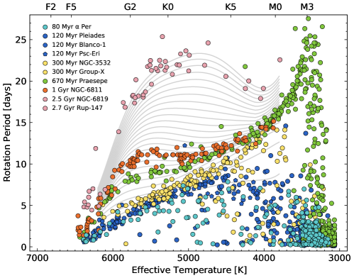
(a)

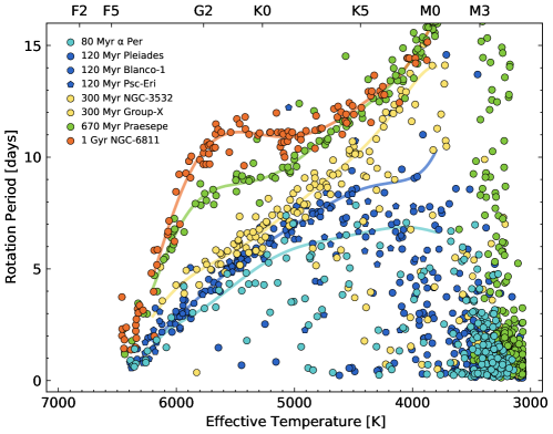
(b)

Figure 1: Open cluster data and models. The top panel shows the data that we aim to model, and the bottom panel focuses on the first gigayear. Gray lines in the top panel show the mean model for the rotation period distribution, and are uniformly spaced at integer multiples of 100 Myr. They are evaluated using a seventh-order polynomial for each cluster (colored lines, bottom panel), and interpolated piecewise between those reference loci. The model is defined over temperatures of 3800–6200 K, and ages of 0.08–2.6 Gyr. Data behind the Figure are available as a machine-readable table.

2.4 The Single-Star Calibration Sequence

Figure 1 is the result of the data curation process described in Sections 2.1 through 2.3. While we have omitted the possible binaries described in Section 2.3 for visual clarity, they are included in the Data behind the Figure. The gray lines are derived from polynomial fits that we describe in the following section. Comparing against the rotation–color sequences in say Godoy-Rivera et al. (2021), it is impressive how sparse the fast sequence is for hot stars. In the 120 Myr clusters, both Blanco-1 and Psc-Eri have no apparently single fast rotators hotter than 5000 K. The Pleiades has four. The rapid rotator sequence is similarly sparse at 300 Myr. The large binary fraction of fast-sequence stars warrants future analysis, to understand whether the binary separations and mass ratios for these systems are typical of the field binary population.

3 A Gyrochronology Model

Here we present a model that aims to accurately describe the evolving rotation period distributions of F7–M0 dwarfs with ages of 0.08–2.6 Gyr. The goal is to then use this model to assess the precision with which rotation periods can be used to infer ages. To perform this analysis, our model needs to account for the trends visible in Figure 1: stellar spin-down rates vary with both mass and age; stellar spin-down can stall; and higher-mass stars younger than Praesepe tend to converge to the slow sequence before lower-mass stars. Our approach will ultimately use interpolation, based on the logic that there are certain regions of Figure 1 in which a hypothetical star located between two cluster sequences would need to have an age intermediate to those two clusters. A few formalities are needed to make this idea rigorous.

3.1 Formalism

For a given star, we have an observed rotation period $\bm{\tilde{}}{P}_{\rm rot}$ and stellar effective temperature $\bm{\tilde{}}{T}_{\rm eff}$ with measurement uncertainties $\sigma_{\bm{\tilde{}}{P}_{\rm rot}}$ and $\sigma_{\bm{\tilde{}}{T}_{\rm eff}}$. Given these data, we want to find the posterior probability distribution for the age $t$ of the star. We write the corresponding probability density as $p(t|\bm{D})$, where $\bm{D}=\{\tilde{P}_{\rm rot},\bm{\tilde{}}{T}_{\rm eff}\}$ are the observed data. We find $p(t|D)$ by marginalizing over the joint probability density $p(t,P_{\rm rot},T_{\rm eff}|D)$, where $P_{\rm rot}$ and $T_{\rm eff}$ are the true rotation period and temperature of the star. Mathematically, this means 1(NOTE DURING EDIT1: Here and for the remaining manuscript, the probability notation was updated from the mathematician’s $f_{x|y}$ to the astronomer’s $p(x|y)$. We also omitted the implicit uncertainties “$s$”, and wrote all instances of the observables as $D$.

$$p(t|D)=\iint p(P_{\rm rot},T_{\rm eff},t|D)\ {\rm d}P_{\rm rot}\ {\rm d}T_{\rm eff}.$$ (1)

By Bayes’ rule, the integrand can be written as

$$p(P_{\rm rot},T_{\rm eff},t|D) \propto p(D|P_{\rm rot},T_{\rm eff},t)\cdot p(P_{\rm rot},T_{\rm eff},t)$$ (2)

where the first term is the likelihood and the latter is the prior.

3.2 Likelihood

For the likelihood, we assume that the observed rotation period and temperature have Gaussian uncertainties and are measured independently. In this case,

$$p(D|P_{\rm rot},T_{\rm eff},t) =p(\bm{\tilde{}}{P}_{\rm rot}|P_{\rm rot},T_{\rm eff},t)\cdot p(\bm{\tilde{}}{T}_{\rm eff}|P_{\rm rot},T_{\rm eff},t),$$ (3)

and the temperature and rotation period distributions are specified by $\bm{\tilde{}}{T}_{\rm eff}\sim\mathcal{N}(T_{\rm eff},\sigma_{\bm{\tilde{}}{T}_{\rm eff}}^{2})$ and $\bm{\tilde{}}{P}_{\rm rot}\sim\mathcal{N}(P_{\rm rot},\sigma_{\bm{\tilde{}}{P}_{\rm rot}}^{2})$, where $\mathcal{N}$ denotes the normal distribution. In other words, our likelihood is a product of two normal distributions.

3.3 Prior

The prior is more interesting. By the chain rule,

$$p(P_{\rm rot},T_{\rm eff},t) =p(P_{\rm rot}|T_{\rm eff},t)\cdot\ p(T_{\rm eff})\cdot\ p(t),$$ (4)

where we have assumed $p(T_{\rm eff}|t)=p(T_{\rm eff})$ because in our model, changes in stellar temperature through time are ignored. We assume that age and temperature are uniformly distributed, $t\sim\mathcal{U}(t_{\rm min},t_{\rm max})$ and $T_{\rm eff}\sim\mathcal{U}(T_{\rm eff}^{\rm min},T_{\rm eff}^{\rm max})$, where $(t_{\rm min},t_{\rm max})$, $(T_{\rm eff}^{\rm min},T_{\rm eff}^{\rm max})$ are the limiting ages and temperatures for our model, respectively. We adopt limiting ages of 0 to 2.6 Gyr, and limiting temperatures of 3800 to 6200 K. The upper limit on age is set by the oldest clusters in our dataset (Table 1), and the temperature limits are set to include the regions in which stellar rotation is most correlated with age. While one might imagine a prior on temperature informed by the stellar initial mass function, or a prior on age informed by the star formation history of the Milky Way, the star formation rate has been approximately constant over the past 10 Gyr (e.g., Nordström et al., 2004) and incorporating a stellar mass function would systematically bias already accurate measurements towards lower temperatures. We do not consider such additions.

The remaining term in Equation 4, $p(P_{\rm rot}|T_{\rm eff},t)$, is the core of our model. We propose a functional form for $p(P_{\rm rot}|T_{\rm eff},t)$ that relies on two components. The first component, $\mu_{\rm slow}(T_{\rm eff},t)$, is the rotation period of the star if it were exactly on the slow sequence — this is colloquially the “mean” gyrochronal model for a star’s rotation period prescribed at any age and temperature. The second component is the residual to that mean model — the probability distribution for how far the star’s rotation period is from the slow sequence at any given age and temperature. This model parametrization is motivated by how the observed abundance of rapid rotators changes as a function of both stellar temperature and age.

The Mean Model

To parametrize the slow sequence, we fitted rotation periods in each reference cluster with an $N^{\rm th}$ order polynomial over 3800–6200 K. We manually selected the slow sequence stars to perform this fit using the data behind Figure 1. We investigated the choice of $N$ between 2 and 9, and settled on $N=7$ as a compromise between overfitting and accurately capturing the structure of the Praesepe and NGC-6811 sequences. While lower-order polynomials provide acceptable fits for the 80–300 Myr clusters (e.g., Curtis et al., 2020, Appendix A), for purposes of homogeneity across all clusters we adopted a single polynomial order.

To model the evolution of the slow sequence, we considered a few possible approaches, all based on interpolating between the fitted polynomials (see Appendix A). We ultimately chose at any given temperature to fit 1-D monotonic cubic splines in rotation period as a function of age. This guarantees a smooth increase in the slow sequence envelope while also fitting all available data. Systematic uncertainties associated with this choice are described in Section 5.2. This procedure yielded the gray lines in Figure 1. At times below 80 Myr, we do not extrapolate; we instead let the “mean model” $\mu_{\rm slow}(t,T_{\rm eff})$ equal the lowest reference polynomial rotation period values as set by $\alpha$ Per. This yields posterior distributions that are uniformly distributed at ages below 80 Myr. Possible options regarding extrapolation for older stars are discussed in Appendix A.

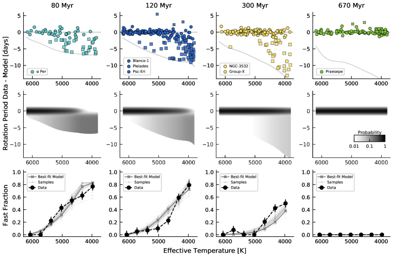
Figure 2: Data, model, and goodness-of-fit. Top: Cluster rotation periods, minus the corresponding slow-sequence mean model at each cluster’s age. The lower gray envelope corresponds to a zero-day rotation period. Middle: Probabilistic model for rotation period as a function of age and temperature (Equation 5), fitted to the 120 Myr, 300 Myr, and 670 Myr clusters. Bottom: Fraction of stars in 350 K bins that rotate “fast”, as a function of temperature. “Fast” and “slow” stars are squares and circles on the top panel; “very slow” outliers are the crosses. “Slow” stars show a uniform scatter of $\sigma$$\approx$0.51 days around the mean model at $t\geq 120$ Myr. The assumed uncertainties for Praesepe are smaller than the markers (see Section 3.5).

The Residual

The top row of Figure 2 shows the residuals for the calibration clusters with $t\leq 670$ Myr, relative to the polynomial model. Our ansatz is to model this distribution as a sum of a Gaussian and a uniform distribution, with each distribution smoothed around a time-dependent transition location in effective temperature. This procedure ignores the few positive outliers.

Mathematically, this means that the rotation period, given the age and temperature, is drawn from

$$P_{\rm rot}\sim \ a_{0}\,\mathcal{N}_{P}(\mu_{\rm slow},\sigma^{2})\otimes L_{T}(T_{\rm eff}^{\rm cut}(t),k_{0})$$ (5)

$$+a_{1}g(t)\ \mathcal{U}_{P}(0,\mu_{\rm slow})\otimes\left(1-L_{T}(T_{\rm eff}^{\rm cut}(t),k_{1})\right),$$

where $\mathcal{N}$ is a normal distribution, $\mathcal{U}$ is a uniform distribution, $a_{0}$ and $a_{1}$ are scaling constants, and $L(\ell,k)$ is the logistic function specified by a location $\ell$ and smoothing scale $k$. Visual examples are given in the middle row of Figure 2. The subscripts, for instance $\mathcal{N}_{P}$, indicate the dimension over which the distribution is defined — period ($P$) or effective temperature ($T$), and $\otimes$ denotes an outer product. We have also hidden the dependence of $\mu_{\rm slow}$ on time and temperature for simplicity of notation.

The first term in Equation 5 parametrizes the slow sequence using a Gaussian centered on $\mu_{\rm slow}(t,T_{\rm eff})$, with a universal width $\sigma=0.51\,{\rm days}$ set by the observations of clusters at least as old as the Pleiades. The location parameter of the logistic function, $T_{\rm eff}^{\rm cut}(t)$, is a function that monotonically decreases to account for the age-dependent transition between the slow and fast sequence. While other functional forms are possible, we assumed that at any given time this function is defined as the temperature of the lowest-mass star that has just arrived at the main-sequence, since this is the time at which the star’s surface rotation rate is no longer affected by gravitational contraction. We evaluated this quantity through linear interpolation over the solar-metallicity MIST grids (Choi et al., 2016). At 80, 120, and 300 Myr this yielded $T_{\rm eff}^{\rm cut}$ values of 4620, 4150, and 3440 K, respectively.

3.4 Free Parameters

The free parameters in the model are as follows. In the residual term, there are the amplitudes $(a_{0},a_{1})$, the two scaling parameters $(k_{0},k_{1})$, and the slope of the linear amplitude decrease $g(t)$ for the “fast sequence” term through time. This would yield five free parameters, but $a_{0}$ and $a_{1}$ are degenerate, so there are really only four degrees of freedom. We fixed the other terms in the model that could in principle be allowed to vary. These included the polynomial terms in the slow sequence model $\mu_{\rm slow}$, the scatter around the slow sequence $\sigma$, and the function specifying the decrease of the effective temperature cutoff through time $T_{\rm eff}^{\rm cut}(t)$.

3.5 Fitting the Model

To compare the model (Equations 1 through 5) to the data, we performed the following procedure. For the reference clusters at 120 Myr ($N_{\star}=196$), 300 Myr ($N_{\star}=133$), and 670 Myr ($N_{\star}=100$), we divided the data into seven bins, starting at 3800 K, with uniform bin widths of 350 K. Including $\alpha$ Per (80 Myr; $N_{\star}=65$) as an optional fourth dataset yielded similar results, so we omitted it for simplicity. In each bin, we counted the number of stars on the slow sequence, and the number of stars on the fast sequence. We considered a star to be “slow” if it is within two days of the mean slow sequence model, and “fast” if it is more than two days faster than the same model. This cutoff was determined based on the uniform scatter of $\sigma\approx 0.51\,$days seen around the slow-sequence for clusters with $t\geq 120$ Myr. We then use the resulting counts to define a “fast fraction,” $F$, the ratio of fast rotating stars to the total number of stars observed in any given temperature bin.

The bottom row of Figure 2 shows this fast fraction as a function of temperature. We calculated the same summary statistic for our model through numerical integration. This yields a $\chi^{2}$ metric, $\chi^{2}=\sum_{i}(F_{i}-F_{i,{\rm model}})^{2}/\sigma_{i}^{2},$ where the sum $i$ is over the three reference sets of open clusters. For the $\sigma_{i}$, the default Poissonian uncertainties would disfavor the small number of stars from 4500–6200 K in Praesepe that are all on the slow sequence. Since auxiliary clusters with similar ages such as the Hyades (Douglas et al., 2019) and NGC-6811 (Curtis et al., 2019a) also have fully converged slow sequences, we adopted a prescription for the $\sigma_{i}$ in which we set them to be equal to one another at 120 and 300 Myr and ten times smaller at 670 Myr. This forces the model to converge to the fast sequence by the age of Praesepe. The normalization of the uncertainties was then allowed to float in order to yield a reduced $\chi^{2}$ of unity.

We fitted the model by sampling the posterior probability using emcee (Foreman-Mackey et al., 2013). We sampled over five parameters: $a_{1}/a_{0}$, $\ln k_{0}$, $\ln k_{1}$, the slope of $g(t)$, and the multiplicative uncertainty normalization. The function $g(t)$ was set to unity below 120 Myr, and to decrease linearly to zero while intersecting 300 Myr at a particular value, $y_{\rm g}$. The latter value was the free parameter used to fit the slope of the line. The maximum-likelihood values yielded by this exercise were $\{a_{1}/a_{0},\ln k_{0},\ln k_{1},y_{\rm g}\}=\{8.26,\scalebox{0.5}[1.0]{$-$}4.88,\scalebox{0.5}[1.0]{$-$}6.24,0.67\}$. To evaluate the posterior, we assumed a prior on each parameter that was uniformly distributed over a wide boundary. We checked convergence by running the chains out to a factor of 300 times longer than the autocorrelation time. The resulting median parameters and their 1$\sigma$ intervals were $\{a_{1}/a_{0},\ln k_{0},\ln k_{1},y_{\rm g}\}=\{9.29_{\scalebox{0.5}[1.0]{$-$}2.41}^{+3.62},\scalebox{0.5}[1.0]{$-$}4.27_{\scalebox{0.5}[1.0]{$-$}1.52}^{+2.56},\scalebox{0.5}[1.0]{$-$}6.15_{\scalebox{0.5}[1.0]{$-$}0.25}^{+0.23},0.63_{\scalebox{0.5}[1.0]{$-$}0.07}^{+0.03}\}$. The lower row of Figure 2 shows the best-fit model plotted over 64 samples. Qualitatively, the model fits the fast fraction’s behavior well in both temperature and time. To check the accuracy of our uncertainties, we performed a cross-validation analysis in which we randomly dropped 20% of the stars in the reference clusters, without replacement, and then refitted the data. The resulting parameters all fell within the stated 1$\sigma$ uncertainty intervals.

3.6 Evaluating the Posterior

For any given star, we numerically evaluate Equation 1 using the composite trapezoidal rule. For each age in a requested grid, we define linear grids in the dimensions of temperature and $y\equiv P-\mu_{\rm slow}$, each with side length $N_{\rm grid}$. The integration is then performed over ${\rm d}T_{\rm eff}$ and ${\rm d}y$ at each specified age. Runtime scales as $\mathcal{O}(N_{\rm grid})$, and takes under a minute on a typical laptop. This runtime estimate however assumes that the four hyperparameters, $a_{1}/a_{0},\ln k_{0},\ln k_{1},$ and $y_{\rm g}$, are fixed. Since these parameters are unknown, the most rigorous approach for age inference for any one star requires sampling from the posterior probability distribution for the hyperparameters. Each sample then yields its own posterior for the age from Equation 1, from which sub-samples can be drawn. All the sub-samples can then be combined to numerically yield an average posterior.

The top panels of Figure 3 show the results of this sampling procedure in dotted lines, plotted underneath an alternative: simply adopting the best-fit model (solid lines). The results are similar, although there are differences for most rapidly rotating stars. While the sampling procedure is relatively simple to parallelize, it is a factor of $\approx$10³ times more expensive than using the best-fit model; for most practitioners, the rigor is unlikely to justify the runtime cost. As we will discuss in Section 5.2, this model has other systematic uncertainties that are more important.

4 Results

4.1 Model Validation

1NOTE DURING EDIT1: This paragraph has been reworded with an updated procedure. Quoted “recovered age” values in the final column of Table 1 have also been updated using the hierarchical bayesian framework. As a validation test, we calculated gyrochronal age posteriors for all 3800–6200 K stars in Figure 1. To infer the implied age for each cluster, we “stack” the posteriors using PosteriorStacker, which considers two hierarchical Bayesian models for the intrinsic age distribution of each cluster: a Gaussian, and a non-parametric histogram. After omitting a few extreme outliers, the two approaches give similar results, and so in the “recovered age” column of Table 1 we report the median and uncertainty of the mean cluster age assuming that the individual stellar ages in each cluster are drawn from a Gaussian. The resulting ages agree with the literature ages for every cluster to within 2$\sigma$, as we would expect for a sample of ten clusters.

As an additional test, we repeated the exercise, but using data for two open clusters outside of our training data: M34 ($\approx$240 Myr; Meibom et al. 2011) and M37 ($\approx$500 Myr; Hartman et al. 2009). For M34, fitting the data after applying the binarity filters described in Section 2.3 yielded an age of $222\pm 20$ Myr. For M37, the same procedure yielded $463\pm 18$ Myr. The latter estimate agrees with the isochronal age found by Hartman et al. (2008) without convective overshoot ($485\pm 28$ Myr), and is 2.5$\sigma$ below their isochronal age that included convective overshoot ($550\pm 30$ Myr).

4.2 Precision of Gyrochronology

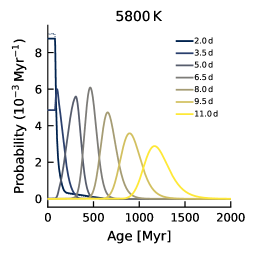
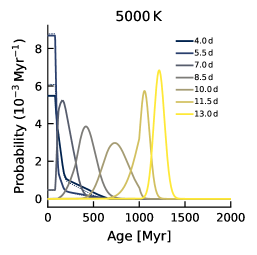
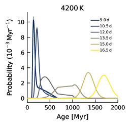
(a)

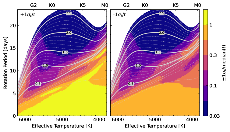
(b)

Figure 3: Precision of gyrochronal ages from our method. Top: Age posteriors across rotation–temperature space. In each subplot, each line represents a pair of $P_{\rm rot}$ and $T_{\rm eff}$, and assumes a precision of 50 K in effective temperature, and 1% in rotation period. The solid lines come from the best-fit model in Figure 2. The under-plotted dotted lines come from a more rigorous approach that samples over the population-level hyperparameters discussed in Section 3.6. Bottom: $+$1$\sigma$ (left) and $-$1$\sigma$ uncertainty (right) of the age posterior, normalized by the median value. For instance “$\pm 1\sigma_{t}/{\rm median}(t)=0.3$” corresponds to 30% relative precision. Thick gray lines are at integer multiples of 500 Myr, and dotted lines are spaced every 100 Myr; labels are in units of gigayears.

Having demonstrated that our method can recover the ages of known cluster stars, here we examine its statistical limits for individual field stars. The bottom panel of Figure 3 shows the $\pm 1$$\sigma$ uncertainties, normalized by the median of the gyrochronal age posteriors, over a grid of rotation periods and temperatures. Broadly speaking, the regions in which rotation periods evolve the least, such as the hottest stars and stalled $\approx$1 Gyr K-dwarfs, have the worst inferred precisions.

The top panel of Figure 3 visualizes vertical slices of the bottom panel for a few canonical cases. For a Sun-like star ($\approx$5800 K) in its early life, the rotation period is only informative in that it provides an upper limit on the star’s age. As the star ages, the age posterior becomes two-sided, with a best-case statistical precision of $\pm 12\%$ at 2 Gyr. For a low-mass K-dwarf, the evolution of the age posterior is more complicated. These stars only converge to the slow sequence by the age of Praesepe. Their spin-down is then observed to stall, which leads to highly asymmetric posteriors between ages of 0.5–1.3 Gyr. For instance, a 4000 K star on the slow-sequence at 200 Myr has a $+1\sigma$ uncertainty of 88%, and a $\scalebox{0.5}[1.0]{$-$}1\sigma$ uncertainty of 13%. Nonetheless, statistical age precisions for such stars are predicted to improve after the era of stalled spin-down, reaching $\pm$9% by 2 Gyr. The implication is that the rotation periods of such stars can be predictive of age, but only at certain times.

5 Discussion & Conclusions

5.1 The Gyrochronal Precision Floor

A key simplifying factor in our analysis is that we assumed the scatter of rotation periods around the slow sequence, $\sigma\approx 0.51\,{\rm days}$, is fixed in time. Based on the data, $\sigma$ appears to be constant between 120 Myr and 1 Gyr (Figure 2, top panel). In $\alpha$ Per, the scatter is larger (0.85 days), likely because the stars are only just converging to the slow sequence. The scatter is also larger in the Ruprecht-147 data, but this is likely due to observational uncertainty in the period measurements. This empirical $\approx$0.51-day scatter could come from a number of sources, including differential rotation on stellar surfaces (Epstein & Pinsonneault, 2014), uncertainties in the effective temperature scale, or differing wind strengths between stars of the same mass and age.

Regardless of the scatter’s origin, it sets the floor for gyrochronal precision, in tandem with the intrinsic spin-down rates. In line with previous results (Barnes, 2007), gyrochronal ages for F-dwarfs are less precise than for G-dwarfs, because F-dwarfs spin down more slowly. However in detail, Figure 3 shows that such statements depend on both mass and age. More broadly, Figure 3 also implies that accounting for the evolving dispersion of the rotation period distributions is a required ingredient for producing accurate age uncertainties.

5.2 Systematic Uncertainties

The uncertainties described thus far have been statistical, rather than systematic. Key systematic uncertainties include the time-varying nature of the spin-down rate, the accuracy of the absolute age scale, and stellar binarity.

Regarding the spin-down rate, our interpolation approach guarantees accuracy near any given reference cluster. However, far from the reference clusters, the choice of interpolation method can affect the inferred ages. We estimated the associated systematic uncertainties by evaluating grids of $P_{\rm rot}$ vs. $T_{\rm eff}$ analogous to Figure 3, but assuming i) piecewise linear interpolation, and ii) piecewise cubic hermite interpolating polynomials calibrated only on the 0.08–2.6 Gyr data (see Appendix A). The difference in the medians of the age posteriors relative to our default interpolation method is an indicator of the systematic uncertainty. This procedure showed a $<$1% bias in the inferred ages for 5000–6200 K stars younger than 1 Gyr, due to the dense sampling of the calibration clusters. For cooler stars however, a linear spin-down rate would yield differences of up to $\pm$15% in the median age due to the rapid spin-down from 0.1–0.3 Gyr (see Figure 1). For older stars between 1 and 2.6 Gyr, the cubic interpolation yielded $\pm$100 Myr differences, while the linear interpolation yielded $-$200 to $+$50 Myr differences, with the largest differences again for stars cooler than 4500 K. The summary is that from 1–2.6 Gyr, there is a 6–12% systematic uncertainty, with the maximum uncertainty at 1.8 Gyr, half-way between the two reference clusters.

Regarding the absolute age scale, Table 1 reports age precisions for the calibration clusters of 3–20%, with the largest uncertainties for the $300\pm 60$ Myr NGC-3532 and Group-X. To assess how shifts in this scale might affect our gyrochronal ages, we again calculated grids of $P_{\rm rot}$ vs. $T_{\rm eff}$, but in this case we shifted all the reference cluster ages by either $+$1$\sigma$ or $-$1$\sigma$. The results showed what one would naively expect: if all the clusters are $\pm$$1$$\sigma$ older than their reference ages, then the changes in the inferred ages match however much freedom there is in the local age scale. For example, for a $5800$ K star with a 5.1 day rotation period, our method statistically yields $t=308^{+70}_{-81}$ Myr, roughly the age of NGC-3532. However, the age of that cluster is uncertain at the 20% level, and so the median age from our estimate for this worst-case scenario could be systematically shifted either up or down by $\pm$20% to match the true age of the reference cluster. From the uncertainties quoted in Table 1, and from comparable studies in the literature (e.g., Dahm, 2015), the age scale itself seems to currently be defined at a $\sim$10% level of accuracy, at best.

Finally, regarding binarity, the presence of even a wide binary during the pre-main-sequence can prompt fast disk clearing, which could alter a star’s rotation period by halting disk-locking (Meibom et al., 2007). This mechanism might explain the abundance of fast rotators in $\approx$120 Myr open clusters (Bouma et al., 2021). A separate concern with binaries is photometric blending of the rotation signal. Because of these issues, our framework is only strictly applicable to stars that are apparently single. Section 2.3 summarizes some of the information that can be used to determine whether a given field star meets this designation. Appendix B discusses the potential impact of ignoring binarity entirely.

5.3 Future Directions

The need for intermediate-age calibrators

The region of Figure 1 with the largest gap, near 1.8 Gyr, has the largest systematic uncertainties in our model. These uncertainties could be addressed by measuring rotation periods in a cluster at this age. Considering clusters from Cantat-Gaudin et al. (2020) older than 1 Gyr, within 1 kpc, and with more than 100 members yields eight objects. Sorted near to far, they are: Ruprecht-147, NGC-752, IC-4756, NGC-6991, NGC-2682, NGC-7762, NGC-2423, and IC-4561. The closest two have been studied by Curtis et al. (2020) and Agüeros et al. (2018), though rotation periods in NGC-752 ($1.34\pm 0.06$ Gyr, $d\sim 440$ pc) could be worth revisiting using data from the Transiting Exoplanet Survey Satellite and the Zwicky Transient Facility. IC-4756 and NGC-6991 could similarly merit further study, though it would be wise to confirm their ages before delving in a rotation period analysis.

Going older

M67 (4 Gyr) will likely be the next rung in the gyrochronology ladder: the analyses by Barnes et al. (2016) and Dungee et al. (2022) have nearly completed its rotation–color sequence. As described in Appendix A, we used their data on M67 to calibrate the rate of spin-down between 1 and 2.6 Gyr. This choice is connected to a generic issue with interpolation-based methods: the systematic uncertainty in the model increases near the boundaries of the interpolation domain. By this logic, incorporating the 4 Gyr data in the most reliable way would require an even older population of stars. Clusters such as NGC 6791 (8 Gyr; Chaboyer et al. 1999), or else a precise set of asteroseismic calibrators (e.g., van Saders et al., 2016) might be the most plausible paths toward this goal, though the complicating effects of stellar evolution bear consideration.

Precision age-dating of field stars

The best way to demonstrate the reliability of a star’s age is to measure it using independent techniques. One framework that we expect to complement our own is the BAFFLES code (Stanford-Moore et al., 2020), which returns age posterior probabilities based on a star’s surface lithium content. Other age-dating tools, including activity (Ca HK, Ca IRT, x-ray, UV excess), isochrones, and asteroseismology, can similarly be combined with our gyrochronal posteriors to verify the accuracy of our rotation-based ages, and to improve on their precision.

Angus et al. (2019) presented an important step in this vein, through a method that simultaneously fitted an isochronal and gyrochronal model to determine a star’s age. Their statistical framework could certainly encompass the model developed in this manuscript. The main advantages of our particular gyrochronology model however are i) improved accuracy for stalling K-dwarfs, ii) improved accuracy in treating the growth of the slow sequence and decay of the fast sequence over the first gigayear, and iii) incorporation of the astrophysical width of the slow sequence for FGK stars. The main disadvantage is that our model is not applicable beyond 2.6 Gyr, though we caution that this is because the calibration data are more sparse in this regime, and so the ages have larger systematic uncertainties.

Physics-based models

A separate issue with our model is that it is empirical, and so it does not yield physical understanding. Physics-based gyrochronology models have provided crucial insight into what gives the data in Figure 1 their structure. The relevant physics likely includes decoupling between the radiative core and convective envelope (Gallet & Bouvier, 2013), angular momentum transport to recouple the core and envelope (Gallet & Bouvier, 2015; Spada & Lanzafame, 2020), and spin-down rates that vary depending on whether the magnetic dynamo is saturated (e.g., Sills et al., 2000; Matt et al., 2015). At older ages, additional physics may well be needed to explain the lethargic spin-down of stars with Rossby numbers comparable to the Sun (Brown, 2014; van Saders et al., 2016; David et al., 2022). A separate issue that also merits attention is the exact role of binarity on stellar rotation. Our filtering process (Section 2.3) removed potential binaries based on a gamut of tracers, because observations have shown that rapid rotators are often binaries (Meibom et al., 2007; Stauffer et al., 2016; Gillen et al., 2020). The exact properties of these binaries, for instance their separations and masses, would help in clarifying the physical origin of this correlation. The issue of whether binarity leads to early disk dispersal seems likely to be related, and also deserves attention (Cieza et al., 2009).

Appendix A Interpolation Methods & Literature Comparison

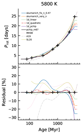
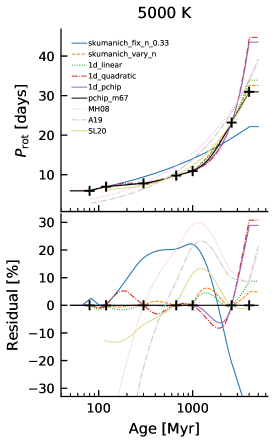
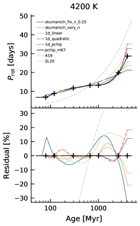
(a)

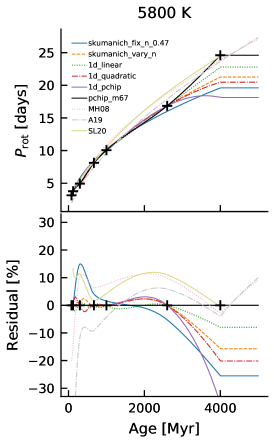
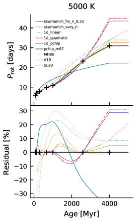
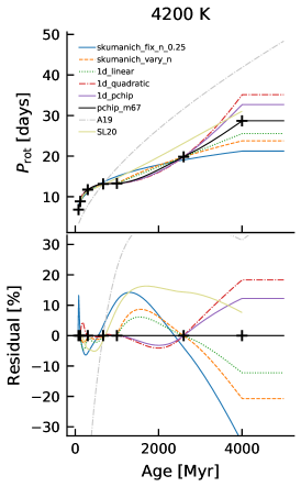
(b)

Figure 4: Different approaches for interpolating between reference clusters. $P_{\rm rot}$ denotes the rotation period of the star if it were evolving exactly along the slow sequence. The top two and bottom two rows show identical data, but are scaled logarithmically and linearly in time. The “residual” is defined versus the pchip_m67 interpolation method, calculated for each model $i$ as $(P_{\rm rot,i}-P_{\rm rot,pchip\_m67})/P_{\rm rot,i}$. The “+” data points are evaluated from polynomial fits to the data in Figure 1. The fixed power laws (“skumanich_fix_n_0.XX”) are extrapolated based on the rotation period at 120 Myr. MH08: Mamajek & Hillenbrand (2008). A19: Angus et al. (2019). SL20: Spada & Lanzafame (2020).

How does the slow sequence evolve between each reference cluster? In other words, what is the functional form of $\mu_{\rm slow}(t,T_{\rm eff})$, the rotation period of a star evolving exactly along the slow sequence? Figure 4 summarizes a few possible answers, evaluated at 5800 K, 5000 K, and 4200 K. Data from Barnes et al. (2016) and Dungee et al. (2022) have been included as the 4 Gyr M67 data points, to assess how well the interpolation methods succeed at extrapolating beyond 2.6 Gyr. As a qualitative note, the stars of interest in this work (0.5–1.2 $M_{\odot}$; 3800–6200 K) have temperature changes of $\lesssim$2.5% between 80 Myr and 2.6 Gyr, according to the MIST grids (Choi et al., 2016). Past $\approx$3 Gyr, the most massive 1.2 $M_{\odot}$ ($\approx 6200$ K) stars begin to turn onto the subgiant branch, and temperature becomes a more ambiguous parameter when modeling stellar spin-down.

The simplest plausible model would be if the slow sequence’s evolution followed a power-law, with a flexible color or temperature calibration similar to that suggested by many authors (e.g., Skumanich, 1972; Noyes et al., 1984; Barnes, 2003). In this approach, for every temperature, we would set $P_{\rm rot}\propto t^{n}$, where canonically $n=1/2$. We would then scale based on some fiducial rotation period, say at 120 Myr. Figure 4 shows how well this type of scaling works, letting $n$ float in order to match the data as well as possible. For Sun-like stars ($\approx$$5800\,$K), this type of scaling works surprisingly well, yielding agreement with the cluster data at the $<$$15$% level for $n=0.47$ out to 4 Gyr. The agreement is significantly worse for lower mass stars, due to their stalled spin-down at intermediate ages.

An alternative approach would be to directly interpolate between the cluster sequences, ignoring our expectation for any kind of power-law spin-down. The resulting linear and quadratic interpolation cases are shown as the dot and dot-dash lines in Figure 4. While these approaches tautologically fit the data, they suffer from sharp transitions in the spin-down rate at every reference cluster. Quadratic interpolation is also not guaranteed to be monotonic, which is probably a desirable property for a stellar spin-down. A final concern is that interpolating in this way is not guaranteed to be predictive; leaving the M67 data out, extrapolating based on the 1–2.6 Gyr data will generally over or under-estimate the rotation periods in the 2.6–4 Gyr interval.

An approach closer to interpolation that still incorporates a form of power-law scaling is as follows. For a point $(T_{i},P_{i})$ intermediate between the loci of two clusters with ages $t_{0}$ and $t_{1}$ and rotation periods $P_{0}$ and $P_{1}$ at the same temperature $T_{i}$, set

$$P_{i} ={P_{0}}\left(\frac{t_{i}}{t_{0}}\right)^{n},\quad{\rm for}\quad n=\frac{\log\left(P_{1}/P_{0}\right)}{\log\left(t_{1}/t_{0}\right)}.$$ (A1)

In other words, given the full set of reference loci $\{\mu_{0},\mu_{1},\ldots,\mu_{k}\}$, their ratios $\{\mu_{1}/\mu_{0},\ldots,\mu_{k}/\mu_{k-1}\}$ can be used to define power-law scalings that are accurate at a piecewise level. While this tautologically fits the data, there is a concern that for cool stars older than 1 Gyr, it may over-estimate the rotation periods. This concern is primarily based on the sharp transition visible in Figure 4 in the spin-down rate at 1 Gyr for the 4200 K case.

A final approach is based on PCHIP interpolation (Piecewise Cubic Hermite Interpolating Polynomials; Fritsch & Butland 1984). This approach is monotonic, and continuous in the first derivatives at each reference cluster. While it is interpolation-based, and therefore not predictive outside of its training bounds, we can include the M67 data in order to define the most accurate possible slow sequence evolution over the 1–2.6 Gyr interval. The results are shown with the black line in Figure 4 in the method labeled “pchip_m67,” which we adopt as our default. This approach leaves the slope of $P_{\rm rot}$ vs. $t$ even less constrained in the 2.6–4 Gyr interval, which is why we do not advocate using our model for stars older than 2.6 Gyr.

Finally, the models from Mamajek & Hillenbrand (2008) (MH08), Angus et al. (2019) (A19), and Spada & Lanzafame (2020) (SL20) are also shown in Figure 4 for comparison. The MH08 model is defined over $0.5<(B-V)_{0}<0.9$, or roughly 5050–6250 K. The $T_{\rm eff}=5000\,{\rm K}$ case is therefore a mild over-extrapolation, but we nonetheless show the result for illustrative purposes. Of the three cases, the Spada & Lanzafame (2020) model generally provides the best match to the data.

Appendix B What if we ignored binarity?

In this work we argued that omitting binaries from gyrochronology analyses is important due to the observational and astrophysical biases that they can otherwise induce on rotation periods. In Section 2.3, we described the set of quality filters that we used to expunge binaries from our calibration data, to guarantee that we were considering only apparently single stars with reliable rotation period measurements. For generic field stars, not all of these conditions are necessarily applicable. For instance, outliers in color–absolute magnitude diagrams might be challenging to identify due to the lack of an immediately obvious reference sequence (although the locus of the main-sequence is itself well-known, and Gaia for instance can now be used to query local spatial volumes around arbitrary field stars to construct well-defined reference samples).

In general, we strongly recommend applying our method only to stars that are thought to be single and on the main sequence. For instance, spectroscopic surface gravity estimates should be used, if available, to expunge evolved stars since they are not in our calibration data. Nonetheless, it is interesting to consider how well our method translates for samples that are messier, and that have binarity rates in line with field populations. Figure 5 shows the result of dropping all of the quality cuts described in Section 2.3, using the data included behind Figure 1.

The first noticeable effect is that without any quality cuts, there are more stars. The star count in $\alpha$ Per jumps from 65 to 128; in the 120 Myr clusters from 196 to 364, in the 300 Myr clusters from 133 to 301; and in Praesepe from 100 to 250. In addition, without quality cuts, the width of the slow sequence increases. The mean residual width for the $t\geq 120$ Myr stars within 2 days of the slow sequence is 0.72 days, a 40% increase from $\sigma=0.51$ days observed in the cleaned sample. This scatter term is proportional to the statistical age uncertainty at late times, in the regime of very precise rotation period and temperature measurements (Barnes, 2007). This suggests that if one wished to apply our gyrochronology model to a population with a mixture of single and binary stars, the model would need to be refit to account for the wider intrinsic scatter in such a population.

Finally, we can ask to what degree the ratio between fast and slow rotators changes when we omit all quality cuts. The results are shown in the bottom row of Figure 5, and compared against the original best-fit model (trained on the cleaned data) from Figure 2. While the visual agreement remains good at $t\geq 120\,$Myr, the hot stars in the raw $\alpha$ Per sample have a larger fast fraction than in the cleaned sample, and so the model provides a worse match to those stars. A second qualitatively important difference is present in Praesepe: the raw data show around a dozen rapid outliers, none of which are present in the cleaned dataset (Figure 2). If any of these stars were single and rapidly rotating, we might construe them as motivation to lengthen our model’s timescale for the decay of the fast sequence. However, since they are most likely binaries, and the Hyades similarly shows no evidence for rapidly rotating single stars hotter than 3800 K (Douglas et al., 2019). The NGC-6811 data at 1 Gyr similarly have no reported rapid rotators (Curtis et al., 2019a). We therefore simply note that these outlying stars do exist at 0.7 Gyr, and that practitioners aiming to perform gyrochronology analyses on populations of stars that include binaries should consider them.

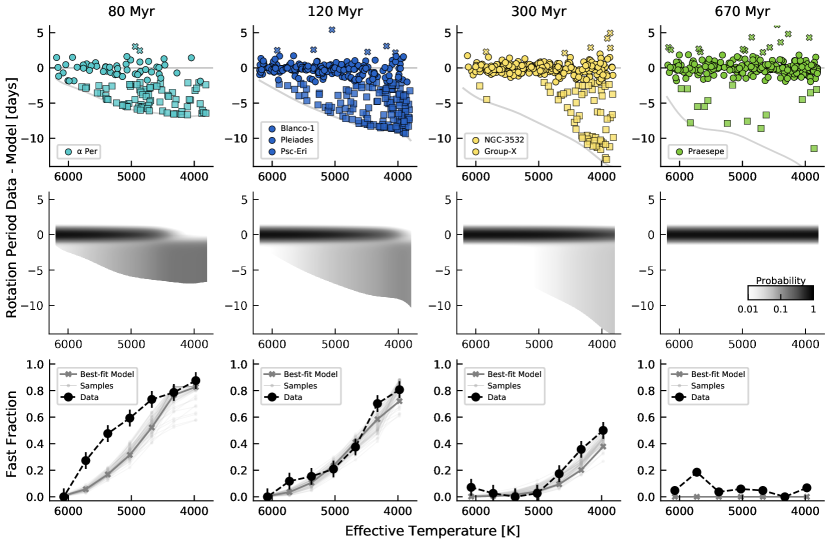
Figure 5: What if we loosened the quality cuts? This plot is the same as Figure 2, but systems that are known or suspected to be visual, photometric, astrometric, and spectroscopic binaries are now displayed along with the single stars. The model is the same as in Figure 2, as is the panel ordering.

References

- Agüeros et al. (2018) Agüeros, M. A., Bowsher, E. C., Bochanski, J. J., et al. 2018, ApJ, 862, 33
- Angus et al. (2019) Angus, R., Morton, T. D., Foreman-Mackey, D., et al. 2019, AJ, 158, 173
- Barnes (2003) Barnes, S. A. 2003, ApJ, 586, 464
- Barnes (2007) —. 2007, ApJ, 669, 1167
- Barnes (2010) —. 2010, ApJ, 722, 222
- Barnes et al. (2016) Barnes, S. A., Weingrill, J., Fritzewski, D., Strassmeier, K. G., & Platais, I. 2016, ApJ, 823, 16
- Baronchelli et al. (2020) Baronchelli, L., Nandra, K., & Buchner, J. 2020, MNRAS, 498, 5284
- Borucki et al. (2010) Borucki, W. J., Koch, D., Basri, G., et al. 2010, Science, 327, 977
- Bouma et al. (2021) Bouma, L. G., Curtis, J. L., Hartman, J. D., Winn, J. N., & Bakos, G. Á. 2021, AJ, 162, 197
- Boyajian et al. (2012) Boyajian, T. S., von Braun, K., van Belle, G., et al. 2012, ApJ, 757, 112
- Boyle & Bouma (2022) Boyle, A. W., & Bouma, L. G. 2022, arXiv e-prints, arXiv:2211.09822
- Brewer et al. (2016) Brewer, J. M., Fischer, D. A., Valenti, J. A., & Piskunov, N. 2016, ApJS, 225, 32
- Brown (2014) Brown, T. M. 2014, ApJ, 789, 101
- Cantat-Gaudin et al. (2020) Cantat-Gaudin, T., Anders, F., Castro-Ginard, A., et al. 2020, A&A, 640, A1
- Chaboyer et al. (1999) Chaboyer, B., Green, E. M., & Liebert, J. 1999, AJ, 117, 1360
- Choi et al. (2016) Choi, J., Dotter, A., Conroy, C., et al. 2016, ApJ, 823, 102
- Cieza et al. (2009) Cieza, L. A., Padgett, D. L., Allen, L. E., et al. 2009, ApJ, 696, L84
- Curtis et al. (2019a) Curtis, J. L., Agüeros, M. A., Douglas, S. T., & Meibom, S. 2019a, ApJ, 879, 49
- Curtis et al. (2019b) Curtis, J. L., Agüeros, M. A., Mamajek, E. E., Wright, J. T., & Cummings, J. D. 2019b, AJ, 158, 77
- Curtis et al. (2020) Curtis, J. L., Agüeros, M. A., Matt, S. P., et al. 2020, ApJ, 904, 140
- Dahm (2015) Dahm, S. E. 2015, ApJ, 813, 108
- David et al. (2022) David, T. J., Angus, R., Curtis, J. L., et al. 2022, ApJ, 933, 114
- Douglas et al. (2019) Douglas, S. T., Curtis, J. L., Agüeros, M. A., et al. 2019, ApJ, 879, 100
- Dungee et al. (2022) Dungee, R., van Saders, J., Gaidos, E., et al. 2022, ApJ, 938, 118
- Epstein & Pinsonneault (2014) Epstein, C. R., & Pinsonneault, M. H. 2014, ApJ, 780, 159
- Foreman-Mackey et al. (2013) Foreman-Mackey, D., Hogg, D. W., Lang, D., & Goodman, J. 2013, PASP, 125, 306
- Fritsch & Butland (1984) Fritsch, F. N., & Butland, J. 1984, SIAM Journal on Scientific and Statistical Computing, 5, 300
- Fritzewski et al. (2019) Fritzewski, D. J., Barnes, S. A., James, D. J., et al. 2019, A&A, 622, A110
- Fritzewski et al. (2021) Fritzewski, D. J., Barnes, S. A., James, D. J., & Strassmeier, K. G. 2021, A&A, 652, A60
- Gaia Collaboration et al. (2022) Gaia Collaboration, Vallenari, A., Brown, A. G. A., et al. 2022, arXiv e-prints, arXiv:2208.00211
- Galindo-Guil et al. (2022) Galindo-Guil, F. J., Barrado, D., Bouy, H., et al. 2022, A&A, 664, A70
- Gallet & Bouvier (2013) Gallet, F., & Bouvier, J. 2013, A&A, 556, A36
- Gallet & Bouvier (2015) —. 2015, A&A, 577, A98
- Gillen et al. (2020) Gillen, E., Briegal, J. T., Hodgkin, S. T., et al. 2020, MNRAS, 492, 1008
- Godoy-Rivera et al. (2021) Godoy-Rivera, D., Pinsonneault, M. H., & Rebull, L. M. 2021, ApJS, 257, 46
- Hartman et al. (2008) Hartman, J. D., Gaudi, B. S., Holman, M. J., et al. 2008, ApJ, 675, 1233
- Hartman et al. (2009) Hartman, J. D., Gaudi, B. S., Pinsonneault, M. H., et al. 2009, ApJ, 691, 342
- Jeffries et al. (2013) Jeffries, Mark W., J., Sandquist, E. L., Mathieu, R. D., et al. 2013, AJ, 146, 58
- Kawaler (1989) Kawaler, S. D. 1989, ApJ, 343, L65
- Mamajek & Hillenbrand (2008) Mamajek, E. E., & Hillenbrand, L. A. 2008, ApJ, 687, 1264
- Mann et al. (2015) Mann, A. W., Feiden, G. A., Gaidos, E., Boyajian, T., & von Braun, K. 2015, ApJ, 804, 64
- Matt et al. (2015) Matt, S. P., Brun, A. S., Baraffe, I., Bouvier, J., & Chabrier, G. 2015, ApJ, 799, L23
- Meibom et al. (2015) Meibom, S., Barnes, S. A., Platais, I., et al. 2015, Nature, 517, 589
- Meibom et al. (2007) Meibom, S., Mathieu, R. D., & Stassun, K. G. 2007, ApJ, 665, L155
- Meibom et al. (2011) Meibom, S., Mathieu, R. D., Stassun, K. G., Liebesny, P., & Saar, S. H. 2011, ApJ, 733, 115
- Messina et al. (2022) Messina, S., Nardiello, D., Desidera, S., et al. 2022, A&A, 657, L3
- Nordström et al. (2004) Nordström, B., Mayor, M., Andersen, J., et al. 2004, A&A, 418, 989
- Noyes et al. (1984) Noyes, R. W., Hartmann, L. W., Baliunas, S. L., Duncan, D. K., & Vaughan, A. H. 1984, ApJ, 279, 763
- Rampalli et al. (2021) Rampalli, R., Agüeros, M. A., Curtis, J. L., et al. 2021, ApJ, 921, 167
- Rebull et al. (2016) Rebull, L. M., Stauffer, J. R., Bouvier, J., et al. 2016, AJ, 152, 114
- Ricker et al. (2015) Ricker, G. R., Winn, J. N., Vanderspek, R., et al. 2015, JATIS, 1, 014003
- Sills et al. (2000) Sills, A., Pinsonneault, M. H., & Terndrup, D. M. 2000, ApJ, 534, 335
- Skumanich (1972) Skumanich, A. 1972, ApJ, 171, 565
- Soderblom (2010) Soderblom, D. R. 2010, ARA&A, 48, 581
- Spada & Lanzafame (2020) Spada, F., & Lanzafame, A. C. 2020, A&A, 636, A76
- Stanford-Moore et al. (2020) Stanford-Moore, S. A., Nielsen, E. L., De Rosa, R. J., Macintosh, B., & Czekala, I. 2020, ApJ, 898, 27
- Stauffer et al. (2016) Stauffer, J., Rebull, L., Bouvier, J., et al. 2016, AJ, 152, 115
- Torres et al. (2020) Torres, G., Vanderburg, A., Curtis, J. L., et al. 2020, ApJ, 896, 162
- van Saders et al. (2016) van Saders, J. L., Ceillier, T., Metcalfe, T. S., et al. 2016, Nature, 529, 181
- Weber & Davis (1967) Weber, E. J., & Davis, Leverett, J. 1967, ApJ, 148, 217
- Wheatley et al. (2018) Wheatley, P. J., West, R. G., Goad, M. R., et al. 2018, MNRAS, 475, 4476